A hidden self-interacting dark matter sector with first order cosmological phase transition and gravitational wave

Abstract

A dark scalar mediator can easily realize the self-interacting dark matter scenario and satisfy the constraint of the relic density of the dark matter. When the hidden sector is highly decoupled from the visible sector, the constraints from direct and indirect detections of dark matter are rather relaxed. The gravitational waves produced by the first order phase transition resulted from this dark scalar mediator will be an important signature to probe such a dark sector. In this work a generic quartic finite-temperature potential is used to induce a strong first order phase transition. A joint analysis of the self-interacting dark matter, the relic density of the dark matter and the first order phase transition shows that the mass range of the dark scalar is about $(4\times 10^{-4}\sim 3)~{}\rm GeV$. For the dark matter, when the temperature ratio $\xi$ between the hidden sector and the visible sector is larger than 0.1, its mass range is found to be $(10~{}\rm MeV\sim 10~{}\rm GeV)$. The produced gravitational waves are found to have a peak frequency of $(10^{-6}\sim 10^{-3})~{}\rm Hz$ for a temperature ratio $0.1<\xi<1$, which may be detectable in future measurements.

I Introduction

The weakly interacting massive particle (WIMP) is the most popular dark matter candidate because its mass is around the electroweak scale and its thermal freeze-out naturally meets the observed relic density. This is the so-called WIMP miracle Bertone:2016nfn ; Lee:1977ua . However, the recent direct detection of dark matter stringently limited the WIMP space, pointing to scenarios beyond the WIMP paradigm. On the other hand, despite of great successes achieved by the standard model of cosmology, i.e., the $\Lambda\rm CDM$ with cold dark matter as the dominant matter component for the evolution of the universe in the large scales, several problems seemingly appeared on the small cosmological scales, such as the core–cusp problem, the diversity problem and the too-big-to-fail problem Tollerud:2014zha ; Garrison-Kimmel:2014vqa ; Navarro:1996gj ; Moore:1999gc ; Oman:2015xda . From the side of particle physics, dark matter feebly interacts with the standard model (SM) particles. This suggests that dark matter may be a part of some hidden sector which almost decoupled from the visible sector at some temperature like the post-inflation reheating period Feng:2008mu ; Berlin:2016gtr in the early universe. If so, the dark matter then froze out from the hidden sector at another specific low temperature with the evolution of the universe. After that, as the universe continued to cool down, the SM particles formed galaxies and the dark matter exists in the universe in the form of halos.

Note that in the above-mentioned hidden sector dark matter scenario, the dark matter can have self-interaction via exchanging a dark mediator. Such self-interacting dark matter (SIDM), unlike the collisionless dark matter in the $\Lambda\rm CDM$, can have elastic scattering between themselves and hence can solve those small-scale problems via the velocity dependence of the self-interacting cross section per unit mass $\sigma/m$ which is about $0.1-10~{}\rm cm^{2}/g$ in different small-scale structures Tulin:2017ara ; Tulin:2013teo . So in this scenario at least two new particles exist in the hidden sector, i.e., the dark matter particle and the dark mediator (scalar or vector)  Bringmann:2020mgx ; Dery:2019jwf . Note that in this case the stability of the dark mediator should also be carefully checked when considering the relic density of dark matter  Duerr:2018mbd ; Kahlhoefer:2017umn . On the one hand, if the decoupling between hidden sector and visible sector is incomplete, the thermal equilibrium may be maintained via the decay of this mediator into the SM particles after the freeze-out of the dark matter. The coupling strength of the portal between hidden sector and visible sector will be severely constrained by the dark matter direct detection. Anyway, the life-time of this mediator will be limited so that it does not spoil the light species abundances predicted by the Big Bang Nucleosynthesis (BBN) Kaplinghat:2013yxa . On the other hand, if hidden sector and visible sector are highly decoupled, it will be much favored because the constraints of dark matter direct detection can be relaxed and both the SIDM paradigm and the demanded dark matter relic density can be realized easily. However, if the mediator is stable, this particle still may dominate the energy density of the early universe in the non-relativistic case  Berlin:2016gtr . In other words, the decay of this mediator into the SM particle are strictly constrained (except that there exist other dark particles which can decay into the SM particles to relax the dark matter direct detection limits) and should be further constrained by the Cosmic Microwave Background (CMB) and BBN Duch:2019vjg . Therefore, the dark matter direct detection, together with CMB and BBN, will stringently constrain the coupling strength of the portal between the hidden sector and visible sector and also constrain the life-time of the portal.

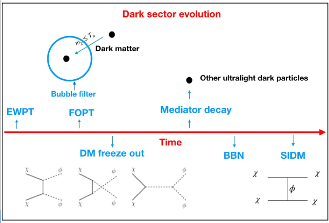
Figure 1: The order of FOPT, freeze out of DM, mediator decay and SIDM in the dark sector evolution history in our work.

In view of a wide variety in the hidden sector, we consider a simple hidden sector with a Dirac fermion dark matter and a scalar to mediate self-interaction of dark matter. We assume the hidden sector to highly decouple from the visible sector. In this scenario, the dark sector can have gravitational waves (GWs) produced by the first order phase transition (FOPT) in the early universe Fairbairn:2019xog ; Breitbach:2018ddu ; Dent:2022bcd ; Marfatia:2020bcs ; Han:2020ekm ; Athron:2019teq ; Kawana:2022lba ; Bian:2021vmi ; Bian:2019kmg ; Hall:2019rld ; Hall:2019ank ; Azatov:2021ifm ; Azatov:2022tii ; Konoplich:1999qq ; Dymnikova:2000dy . Then various constraints on this hidden SIDM, such as from the relic density, will be studied in this work. If a strong FOPT happens, the hidden sector physics can be accessible through the detection of the GWs in the future. The time order of the FOPT, the freeze-out of DM, the mediator decay and the SIDM in the dark sector evolution in our model is shown in Fig. 1. Note that for our hidden SIDM sector, although we only present the dark matter and the dark scalar, this dark scalar must decay into other ultra-light dark particles (say some ultra-light dark fermions) after the dark matter freeze out, which will not affect the dark matter annihilation process and the dark matter relic density. The abundances of the light species in the BBN stage will not be spoiled by the dark particles. This means that when the hidden sector is highly decoupled from the visible sector, other light dark particles must exist unless the dark mediator can decay into some SM particles via the freeze-in mechanism after the dark matter freeze out from the hidden sector. In this work, our focus is the dark matter, which can penetrate the bubble filter of FOPT and satisfy the constraint of relic density, and the dark scalar which can realize the SIDM paradigm and FOPT in the hidden sector. This work is organized as the follows. A benchmark model with cosmological phase transition and gravitational wave is described in Sec. II. The study of the SIDM in this model is given in Sec. III. The numerical results are presented in Sec. VI and the conclusion is given in Section VII.

II A simple model with FOPT in hidden sector

II.1 A benchmark model

If a hidden sector exists, the dark sector can be highly decoupled from the visible sector after the inflation or since the third stage of the reheating at a specific dark temperature. To be simplest, we assume the existence of a dark Dirac fermion $\chi$ as the dark matter and a dark scalar particle $\phi$ with the dark Yukawa interaction Marfatia:2021twj . The Lagrangian is

$$\mathcal{L}\supset\bar{\chi}i\partial\!\!\!/\chi-g_{\chi}\phi\bar{\chi}\chi-V_{eff}(\phi,T),$$ (1)

where $\chi$ has a global $U(1)$ symmetry and $V_{\rm eff}(\phi,T)$ is the finite-temperature effective potential of the field $\phi$. When temperature decreases to a critical temperature $T_{c}$, the universe abruptly traverses from a meta-stable state to another ground state. This means that the scalar field $\phi$ is quantum-tunneling from the false vacuum $\langle\phi\rangle=0$ to the true vacuum $\langle\phi\rangle=v_{\phi}$. As studied in Ref. Hong:2020est , the bubble wall plays a role of a filter during the FOPT. According to the energy conservation, if the mass of $\chi$ in the true vacuum is smaller than its kinetic energy in the false vacuum, all particle can penetrate the bubble wall safely, namely $m_{\chi}\simeq g_{\chi}v_{\phi}\leq T_{n}$ (note $T_{n}$ is the following nucleation temperature $T_{hn}$). Due to no residual dark matter in the false vacuum, the primordial black holes, the Fermi-balls, the Q-balls, or the thermal balls will not be formed Gross:2021qgx ; Huang:2022him ; Baker:2021nyl ; Baker:2021sno ; Huang:2017kzu . Subsequently, we consider the case that the freeze-out dark matter in this hidden sector will account for all the required relic density. To solve the small scale problems by this hidden self-interacting dark matter, the mass of scalar mediator $\phi$ is above MeV, as found in our following study, which is larger than the photo temperature at neutrino decoupling Breitbach:2018ddu . As a result, the cosmological constraints such as CMB and BBN can be avoided during the FOPT in our analysis.

II.2 Cosmological phase transition and gravitational waves

Superficially, our SIDM model is kind of ’effective’ description which just contains a dark Dirac fermion $\chi$ as the dark matter and a dark scalar particle $\phi$. In a complete theory, the particles in the hidden sector could be similar to the visible sector, i.e., with additional dark particles like the right-handed neutrinos DiBari:2021dri and the dark complex scalars in various supersymmetric models Wang:2022lxn ; Huang:2014ifa . Meanwhile, after the dark matter freeze out, the dark mediator must decay into other light dark particles. The light species abundances in the BBN stage will not be spoiled by the dark particles. Since our model is only an ’effective’ description, we choose a generic form of the quartic finite-temperature potential for the dark scalar Adams:1993zs ; Kehayias:2009tn

$$V_{\rm eff}(\phi,T_{h})=D(T_{h}^{2}-T_{h0}^{2})\phi^{2}-(AT_{h}+C)\phi^{3}+\frac{\lambda}{4}\phi^{4},$$ (2)

where $D$, $A$ and $\lambda$ are dimensionless parameters, $C$ provides the cubic term at zero temperature and $T_{h}$ is the temperature of the hidden sector. Simply, the minimal value of the potential is located at

$$v_{0\pm}=\frac{3C\pm\sqrt{9C^{2}+8\lambda DT_{h0}^{2}}}{2\lambda},$$ (3)

Note that here is the zero temperature case, $T_{h}=0$. The mass of the scalar particle at zero temperature is obtained from the second derivative of $V(\phi,0)$ with respect to $\phi$

$$m_{\phi}=\frac{d^{2}V_{\rm eff}(\phi,0)}{d\phi^{2}}\Big{|}_{\phi=v_{0+}}=4DT_{h0}^{2}+3Cv_{0+}\,.$$ (4)

The critical temperature is obtained from $V(0,T_{c})=V(v(T_{c}),T_{c})$

$$T_{hc}=\frac{-CA-\sqrt{D\lambda(C^{2}-(A^{2}-D\lambda)T_{h0}^{2})}}{A^{2}-D\lambda}.$$ (5)

The corresponding scalar field value will be

$$\phi_{T_{hc}}=\frac{3C+3AT_{h}+\sqrt{(-3C-3AT_{h})^{2}-4(2dT_{h}^{2}-2dT_{h0}^{2})\lambda}}{2\lambda}.$$ (6)

Note that $A^{2}-D\lambda<0$ is required for a real critical temperature $T_{hc}$.

During the FOPT process, the decay probability per unit time per unit volume is

$$\Gamma\sim T_{h}^{4}\left(\frac{S_{3}(T_{h})}{2\pi T_{h}}\right)^{3/2}e^{-S_{3}(T_{h})/T_{h}},$$ (7)

where the Euclidean action $S_{3}(T)$ is written as

$$S_{3}=\int_{0}^{\infty}4\pi r^{2}dr\left[\frac{1}{2}\left(\frac{d\phi}{dr}\right)^{2}+V_{\rm eff}(\phi,T_{h})\right].$$ (8)

To evaluate $S_{3}$, the $\mathcal{O}(3)$ symmetric equation of motion needs to be solved, namely,

$$\frac{d^{2}\phi}{dr^{2}}+\frac{2}{r}\frac{d\phi}{dr}=\frac{\partial}{\partial\phi}V_{\rm eff}(\phi,T_{h}),\quad\lim_{r\to\infty}\phi=0,\quad\frac{d\phi}{dr}\Big{|}_{r=0}=0.$$ (9)

For a three-dimensional Euclidean action, it can be derived from a quartic potential

$$V_{\rm eff}(\phi,T_{h})\simeq\bar{\lambda}\phi^{4}-a\phi^{3}+b\phi^{2},$$ (10)

These parameters are given as

$$\bar{\lambda}=\lambda/4,$$ (11)

$$a=AT_{h}+C,$$ (12)

$$b=D(T^{2}_{h}-T^{2}_{h0}).$$ (13)

The corresponding semi-analytic approximate $S_{3}$ is given by

$$S_{3}(T_{h})=\frac{\pi a}{\bar{\lambda}^{\frac{3}{2}}}\frac{8\sqrt{2}}{81}(2-\delta)^{-2}\sqrt{\frac{\delta}{2}}(\beta_{1}\delta+\beta_{2}\delta^{2}+\beta_{3}\delta^{3}),$$ (14)

with $\delta=8\bar{\lambda}b/a^{2}$, $\beta_{1}=8.2938$, $\beta_{2}=-5.5330$ and $\beta_{3}=0.8180$ Adams:1993zs .

The probability for a bubble to nucleate inside a Hubble volume is

$$N(T_{h})=\int_{T_{h}}^{T_{hc}}\frac{dT^{\prime}_{h}}{T^{\prime}_{h}}\frac{\Gamma(T^{\prime}_{h})}{H^{4}(T^{\prime}_{h})},$$ (15)

where $H(T_{h})$ is the Hubble constant. When $N(T_{hn})\sim 1$, the solved temperature is called the nucleation temperature $T_{hn}$. For a FOPT around $\mathcal{O}(100\text{GeV})$, the nucleation temperature can be approximately taken as  Quiros:1999jp

$$S_{3}(T_{hn})/T_{hn}\simeq 140,$$ (16)

which is called as the electroweak phase transition and , this value can be derived from the following Eq.(17). In fact, the nucleation temperature is not necessarily at the electroweak scale, whose criterion can be expressed as Imtiaz:2018dfn

$$\frac{S_{3}}{T_{hn}}\simeq\ln[\frac{1}{4}(\frac{90}{8\pi^{3}g_{\rm eff}})^{2}]+4\ln[\frac{M_{pl}}{T_{hn}}].$$ (17)

Here, $T_{hn}$ on the right-hand side is taken place by $T_{hc}$ approximately due to the logarithmic function.

In the FOPT, the parameter $\alpha$ denotes the strength of the phase transition, which is read as

$$\alpha=\frac{(1-T\frac{\partial}{\partial T_{h}})\Delta V\big{|}_{T_{h*}}}{\rho_{r}},$$ (18)

where $\Delta V=V_{\rm eff}(0,T_{h})-V_{\rm eff}(v_{\phi}(T_{h}),T_{h})$ and the radiation energy density is $\rho(T_{h})=\frac{\pi^{2}}{30}g_{*}T^{4}_{SM}$ with $g_{*}=g_{*SM}+g_{*D}(\frac{T_{h}}{T_{SM}})^{4}$ . We take $g_{*D}=4.5$ at all relevant time and $g_{*SM}$ can be found in  Husdal:2016haj . Because the energy of FOPT we are interested in is above MeV, the temperature ratio between hidden sector and visible sector is not constrained by the BBN or CMB. Another parameter is the inverse duration of the phase transition which can be written as

$$\beta=\frac{\dot{\Gamma}}{\Gamma}\simeq-\frac{d(\frac{S_{3}}{T_{h}})}{dt}\big{|}_{t=t_{h*}}.$$ (19)

In the GW calculation, it is expressed as

$$\frac{\beta}{H_{*}}\simeq T_{h*}\frac{d(\frac{S_{3}}{T_{h}})}{dT_{h}}\big{|}_{T_{h*}}$$ (20)

Generally, a bigger $\alpha$ and a smaller $\beta$ imply a stronger FOPT.

Then the main way to generate stochastic GWs in the FOPT includes bubble collision, sound waves and turbulence of the magneto-hydrodynamics (MHD) in the particle bath. Due to the friction the motion of bubble walls will be significantly dampened in the plasma-wall system. So the wall will reach a terminal velocity $v_{b}$ at a very short time. Therefore, the bubble collision contribution is negligible. Note that our work focuses on CPT and GW, so we consider that when bubble walls collide, the thickness of walls will be very thin. Thus this process does not form a PBH Jung:2021mku . Certainly, under certain conditions, the closed walls may eventually collapse into primordial black holes. However, the abundance of these primordial black holes should not be very large so that it does not contradict the observations Deng:2016vzb ; Belotsky:2018wph ; Rubin:2001yw ; Carr:2019bel . On the flip side, most of energy is pumped into the fluid shells surrounding the wall Ellis:2018mja ; Wang:2020jrd . Finally the significant contribution source of the GWs is from the sound waves while the contribution of the MHD turbulence is a sub-leading source for the GWs. The GW spectrum is

$$\Omega_{\rm GW}(f)=\frac{1}{\rho_{c}}\frac{\rho_{\rm GW}}{d\ln f},$$ (21)

where $f$ is the frequency, $\rho_{\rm GW}$ is the GW energy density produced during FOPT and $\rho_{c}$ is the critical energy density of the present universe. The total GW spectrum is written as

$$\Omega_{\rm GW}h^{2}\simeq\Omega_{\rm sw}h^{2}+\Omega_{\rm turb}h^{2},$$ (22)

where the sound wave contribution is written as

$$h^{2}\Omega_{\rm sw}(f)=2.65\times 10^{-6}(H_{n}\tau_{\rm sw})\left(\frac{H_{n}}{\beta}\right)\left(\frac{\kappa_{v}\alpha}{1+\alpha}\right)^{2}\left(\frac{100}{g_{*}}\right)^{\frac{1}{3}}v_{b}S_{\rm sw}(f),$$ (23)

$$S_{\rm sw}(f)=\left(\frac{f}{f_{\rm sw}}\right)^{3}\left(\frac{7}{4+3(\frac{f}{f_{\rm sw}})^{2}}\right)^{\frac{7}{2}},$$ (24)

$$f_{\rm sw}=1.9\times 10^{-2}~{}{\rm mHz}\frac{1}{v_{b}}\left(\frac{\beta}{H_{n}}\right)\left(\frac{T_{hn}}{100~{}{\rm GeV}}\right)\left(\frac{g_{*}}{100}\right)^{\frac{1}{6}},$$ (25)

with $\tau_{\rm sw}$ being the duration of the sound wave source and $\kappa_{v}$ being the ratio of the bulk kinetic energy to the vacuum energy  Espinosa:2010hh ; Wang:2020jrd . The turbulence contribution is written as

$$h^{2}\Omega_{{\rm turb}}(f)=3.35\times 10^{-4}(\frac{H_{n}}{\beta})(\frac{\kappa_{\rm turb}\alpha}{1+\alpha})^{2}(\frac{100}{g_{*}})^{\frac{1}{3}}v_{w}S_{\rm sturb}(f)$$ (26)

$$S_{\rm turb}(f)=\frac{(\frac{f}{f_{\rm turb}})^{3}}{[1+(\frac{f}{f_{\rm turb}})]^{\frac{11}{3}}(1+\frac{8\pi f}{h_{p}})}$$ (27)

$$f_{\rm sw}=2.7\times 10^{-2}{\rm mHz}\frac{1}{v_{w}}(\frac{\beta}{H_{n}})(\frac{T_{hn}}{100Gev})(\frac{g_{*}}{100})^{\frac{1}{6}}$$ (28)

$$\kappa_{\rm turb}=\epsilon\kappa_{v}.$$ (29)

Here $\epsilon$ represents the fraction of bulk motion which is turbulent and $H_{n}$ is the Hubble parameter at $T_{hn}$.

III Dark matter relic density and self-interaction

III.1 Dark matter relic density

After the dark matter safely penetrates the bubble walls, the FOPT can be considered as decoupling from the freeze-out process of the dark matter Chao:2020adk . In contrast with the usual WIMP freeze-out mechanism Liu:2013vha , the Boltzmann equation needs to be modified in some aspects, e.g., the equilibrium density $n_{\rm eq}$ and the thermal average $\langle\sigma v\rangle$ are evaluated at the dark temperature $T_{h}$ rather than the SM temperature $T$ and the Hubble parameter must be included in the energy of the dark sector Bringmann:2020mgx . Next we examine the dark matter relic density when the hidden sector and the visible sector are at different temperature. Here the temperature ratio is defined as $\xi=T_{h}/T$. The cosmological evolution of the dark matter is determined by the following Boltzmann equation which takes a similar form as in the WIMP paradigm:

$$\frac{dn_{\chi}}{dt}+3Hn_{\chi}=\langle\sigma v\rangle((n_{\chi}^{\rm eq})^{2}-n_{\chi}^{2}),$$ (30)

where the equilibrium number density is in the non-relativistic limit

$$n^{\rm eq}_{\chi}=g_{\chi}(\frac{\xi m_{\chi}T}{2\pi})^{\frac{3}{2}}e^{-\frac{m_{\chi}}{\xi T}}.$$ (31)

The Hubble parameter during radiation domination is given by

$$H^{2}=\frac{8\pi^{3}}{90}g_{\rm eff}M^{-2}_{\rm PI}T^{4},$$ (32)

where the total effective relativistic energy degree-of-freedom (d.o.f) $g_{\rm eff}=g_{\rm SM}+(\sum_{b}g_{b}+\frac{7}{8}\sum_{f}g_{f})\xi^{4}$ with $g_{b}$ and $g_{f}$ being respectively the intrinsic d.o.f of bosons (b) and fermions (f) in the dark sector. In our work, we take $g_{b}=1$ and $g_{f}=3.5$ for numerical calculations.

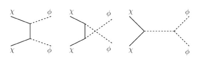
Figure 2: The Feynman pictures from three annihilation processes $\chi\chi\rightarrow\phi\phi$

In the non-relativistic regime, according to the Feynman diagrams in FIG. 2, the approximate thermal average pair annihilation cross section of the dark matter is

$$\langle\sigma v\rangle=a+b\langle v^{2}\rangle=a+6\xi b\frac{T}{m_{\chi}},$$ (33)

where $a$ is the $s$-wave cross section and $b$ is the $p$-wave cross section. In this scenario, $\langle\sigma v\rangle$ is given by  Shtabovenko:2016sxi ; Shtabovenko:2020gxv

$$\begin{split}\langle\sigma v\rangle=&\frac{mv^{2}}{96\pi(m_{\phi}^{2}-2m_{\chi}^{2})^{4}(m_{\chi}m_{\phi}^{2}-4m_{\chi}^{3})^{2}}g_{\chi}^{2}\sqrt{(m_{\chi}-m_{\phi})(m_{\chi}+m_{\phi})}\\ &\times(3C^{2}(m_{\phi}^{2}-2m_{\chi}^{2})^{4}+4Cg_{\chi}m_{\chi}(28m_{\chi}^{4}-11m_{\chi}^{2}m_{\phi}^{2}+m_{\phi}^{4})(m_{\phi}^{2}-2m_{\chi}^{2})^{2}\\ &+8g_{\chi}^{2}m_{\chi}^{2}(m_{\phi}^{2}-4m_{\chi}^{2})^{2}(9m_{\chi}^{4}-4m_{\chi}^{2}m_{\phi}^{2}+m_{\phi}^{4})).\end{split}$$ (34)

This implies that the annihilation is dominated by $p$-wave process.

As studied in  Chacko:2015noa , the freeze out temperature can be evaluated by

$$x_{f}=\xi\log[\frac{c(c+2)}{4\pi^{3}}\sqrt{\frac{45}{2}}\frac{g_{\chi}}{\sqrt{g_{*\rm eff}}}m_{\chi}M_{\rm pl}\frac{\xi^{\frac{5}{2}}\langle\sigma v\rangle}{\sqrt{x_{f}}}]$$ (35)

where $x_{f}=m_{\chi}/T$, and $c=\sqrt{2}-1$ is for $s$-wave annihilation and $c=\sqrt{3}-1$ is for $p$-wave annihilation. Finally, the dark matter relic density is given by

$$\Omega_{\rm DM}h^{2}=m_{\chi}s_{0}Y_{\infty}\rho^{-1}_{c},$$ (36)

in which

$$Y_{\infty}=\frac{x_{f}}{\sqrt{\frac{\pi}{45}}\frac{g_{*}}{g_{\rm eff}^{1/2}}M_{\rm pl}m_{\chi}(a+3\xi b/x_{f})},$$ (37)

and $s_{0}$ and $\rho_{c}$ are the entropy density and critical density at present time, respectively.

III.2 Dark matter self-interaction

As mentioned above, an appropriate self-interaction between the dark matter particles can give the required scattering cross section per unit mass $\sigma/m$ Kim:2022cpu ; Kim:2021bmx ; Bringmann:2016din ; Chu:2018fzy . Especially, the interaction through a light mediator may give a specific required velocity-dependence for different small scale objects. Note that another source of velocity-dependence can be obtained by including the finite-size effect Chu:2018faw ; Wang:2021tjf . The transfer cross section is written as

$$\sigma_{\rm T}\equiv\int d\Omega\,(1-\cos\theta)\frac{d\sigma}{d\Omega}.$$ (38)

Generally, this cross section should be obtained by solving the Schrödinger equation numerically. In our work, the calculation method shown in Colquhoun:2020adl is used. Two dimensionless parameters $\kappa$ and $\beta$ are used to delineate different regimes such as the Born ($2\beta\kappa^{2}\ll 1$), the quantum ($\kappa\ll 1$) and the semi-classical ($\kappa\geq 1$). These two parameters are

$$\kappa=\frac{m_{\chi}v}{m_{\phi}},\quad\quad\beta=\frac{2\alpha m_{\phi}}{m_{\chi}v^{2}}.$$ (39)

The analytic formulas of the transfer cross section in the semi-classical regime ($\kappa\geq 1$) for an attractive Yukawa potential are given by  Colquhoun:2020adl

$$\sigma_{T}^{\rm{att}} =\frac{\pi}{m_{\phi}^{2}}\times\begin{cases}2\beta^{2}\zeta_{1/2}\left(\kappa,\beta\right)&\beta\leq 0.2\\ \hskip 199.16928pt\ &\\[-11.66563pt] 2\beta^{2}\zeta_{1/2}\left(\kappa,\beta\right)e^{0.64(\beta-0.2)}&0.2<\beta\leq 1\\ \hskip 199.16928pt\ &\\[-11.66563pt] 4.7\log(\beta+0.82)&1<\beta<50\\ \hskip 199.16928pt\ &\\[-11.66563pt] 2\log\beta(\log\log\beta+1)&\beta\geq 50,\end{cases}$$ (40)

where

$$\zeta_{n}(\kappa,\beta) =\frac{\text{max}(n,\beta\kappa)^{2}-n^{2}}{2\kappa^{2}\beta^{2}}+\eta\left(\frac{\text{max}(n,\beta\kappa)}{\kappa}\right)\,,$$ (41)

$$\eta(x) =x^{2}\left[-K_{1}\left(x\right)^{2}+K_{0}\left(x\right)K_{2}\left(x\right)\right]\,,$$ (42)

with $K_{n}$ being the modified Bessel function of the second kind. In case of $\kappa<0.4$, the Schrödinger equation can be solved analytically via the Hulthén potential since this quantum regime is dominated by $s$-wave scattering Tulin:2013teo ,

$$\sigma_{T}^{\mbox{Hulth\'{e}n}}=\frac{16\pi}{m_{\chi}^{2}v^{2}}\sin^{2}\delta_{0},$$ (43)

where the phase shift $\delta_{0}$ is

$$\begin{split}\delta_{0}&=\arg\left(i\frac{\Gamma(l_{+}+l_{-}-2)}{\Gamma(l_{+})\Gamma(l_{-})}\right),\\ l_{+}&=1+\frac{\kappa}{1.6}(i+i\sqrt{3.2\beta\pm 1}),\\ l_{-}&=1-\frac{\kappa}{1.6}(i+i\sqrt{3.2\beta\pm 1}).\end{split}$$ (44)

Here the signs $+(-)$ denotes repulsive (attractive). When $\kappa$ is in the range $(0.4,1)$, as shown in Colquhoun:2020adl , the interpolation function is used, namely,

$$\sigma_{T}=(1-\kappa)/0.6\sigma_{T}^{\mbox{Hulth\'{e}n}}+(\kappa-0.4)/0.6\sigma_{T}^{\rm{rep(att)}}.$$ (45)

Thus, the entire interesting parameter space of SIDM can be almost covered analytically. Using the Maxwell-Boltzmann distribution, we can get the the velocity-averaged transfer cross section

$$\langle\sigma_{T}v\rangle=\int f(v)\sigma_{T}vdv$$ (46)

$$f(v)=\frac{32v^{2}e^{-4v^{2}/\pi\langle v\rangle^{2}}}{\pi^{2}\langle v\rangle^{3}}$$ (47)

where $v$ is the relative velocity in the center-of-mass frame.

IV Numerical results

In this section we show the numerical results of the FOPT and the constraints on SIDM including the attractive Yukawa potential and dark matter relic density. We will concentrate on the favored mass parameter space of the dark matter and the scalar particle.

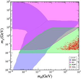
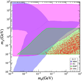
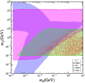
Figure 3: The parameter space of $m_{\phi}$ and $m_{\chi}$ for different temperature ratio $\xi=0.01,0.1,1$. The shadow areas correspond to three constraints: SIDM (blue for attractive Yukawa potential), dark matter relic density (magenta) and FOPT (green). The red scatter points are for the produced GWs with power spectrum $\Omega_{\rm GW}h^{2}>10^{-20}$.

First, in the SIDM scenario for an attractive Yukawa potential, the input parameters include the masses of dark matter $m_{\chi}$ and dark scalar $m_{\phi}$ as well as the dark Yukawa coupling constant $g_{\chi}$. These parameters vary in the ranges

$$10^{-4}~{}{\rm GeV}<m_{\chi}<10^{4}~{}{\rm GeV},\quad 10^{-4}~{}{\rm GeV}<m_{\phi}<10^{4}~{}{\rm GeV},\quad 10^{-3}<g_{\chi}<1$$ (48)

To solve the small-scale structure anomalies, the value of $\sigma_{T}/m_{\chi}$ in the range $(0.1,10~{}\rm cm^{2}/g)$ is favored. Then the favoured regions of the masses $m_{\chi}$ and $m_{\phi}$ are shown as the blue part in Fig. 3. It shows a significant mass split between those two dark particles. Unlike the results in Ref. Tulin:2013teo which gives an allowed parameter space of $m_{\phi}$ in ($1\sim 100$) MeV, here the allowed mass space is larger for the attractive SIDM case. The reason is that our model has a more completed self-interaction in the hidden sector. Another point should be noted is that the resonant effect is very obvious and the three panels of Fig. 3 imply that the up bound for $m_{\phi}$ is about 10 GeV. For the input parameters during the FOPT, we choose

$$\begin{split}&10^{-4}<A<10^{4},\quad 10^{-4}<D<10^{4},\quad 10^{-4}~{}{\rm GeV}<T_{0}<10^{4}~{}{\rm GeV},\quad\\ &10^{-4}~{}{\rm GeV}<C<1~{}{\rm GeV},\quad 10^{-4}<\lambda<1.\end{split}$$ (49)

The corresponding numerical results are shown in the green area in Fig.  3. For the FOPT the maximum mass of dark matter $m_{\chi}\simeq T_{n}$ is taken. For example, for a benchmark point with $m_{\chi}=0.22322$ and $v_{\phi}=1.6682$, we have $g_{\chi}=0.13381$. The different $\xi$ values almost have no influence for the selection of dark particle mass. The combination of SIDM and FOPT requires $m_{\chi}$ in the range of $(10^{-2}\sim 10)$ GeV.

Finally we show the constraints from the dark matter relic density $\Omega_{\rm DM}h^{2}\in(0.11,0.13)$. Now we have one more coupling coefficient $C$, which denotes the cubic term in Eq.(2), and we set it in the range of $(10^{-3}\sim 1)$ GeV. As the initial temperature ratio between those two sectors after the reheating is unknown, we simply take the temperature ratio $\xi=0.01,0.1,1$ for the calculation of the dark matter relic density. The numerical results are shown in the magenta region of Fig. 3, which indicate that the lowest bound for $m_{\chi}$ is higher than $3\times 10^{-3}$ GeV when the hidden sector is colder than the visible sector. In all, the SIDM and the relic density of dark matter can be satisfied by the sub-GeV dark scalar and in this hidden sector the FOPT can happen. To achieve all these, the mass space is about $m_{\chi}\in(0.01\sim 10)$ GeV and $m_{\phi}\in(4\times 10^{-4}\sim 3)$ GeV when the hidden sector is colder than the visible sector, as shown by the gray (overlapped) region in Fig. 3. When the value of $\xi$ is smaller, the survived space of $m_{\chi}$ becomes narrower. Note that in our study the dark matter froze out after the FOPT so that its relic density is not diluted by the FOPT Xiao:2022oaq .

In order to find out whether the GWs produced by FOPT can be detected, we calculate the GW power spectrum $\Omega_{\rm GW}h^{2}$ in the parameter space $m_{\chi}\in(0.01\sim 10)$ GeV and $m_{\phi}\in(4\times 10^{-4}\sim 3)$ GeV which satisfy the FOPT. Then the corresponding GW power spectrum $\Omega_{\rm GW}h^{2}>10^{-20}$ is plotted as red points in Fig. 3. We can see that the red points are excluded by the constraint of dark matter relic density for $\xi=0.01,0.1$, indicating that the GW power spectrum cannot be detected by current detectors. This is because the latent energy is quite small in these cases. Instead, for $\xi=1$ there survived some red points allowed by all constraints, which implies that produced GWs may be detectable by SKA, THEIA, BBO, LISA, TianQin or DECIGO, as shown in Fig. 4. As the peak frequency increases, the power $\Omega_{\rm GW}$ decreases. In brief, for a temperature ratio $\xi$ smaller than $0.1$ the GW is not detectable; the detectable GW has a peak frequency of ($10^{-6}\sim 10^{-3}$) Hz for the hidden sector physics.

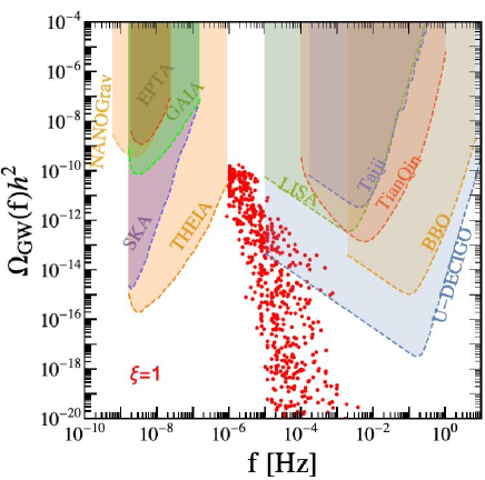
Figure 4: The GW power spectrum $\Omega_{\rm GW}(f)h^{2}$. The red points denote the GWs produced by the FOPT of our model for a temperature ratio $\xi=1$. The detectable regions of various GW detectors are shown as the shadow areas.

In summary, with all constraints we find that the allowed dark matter mass space is about $(0.01\sim 10)$ GeV and the dark scalar mass is $(4\times 10^{-4}\sim 3)$ GeV for an attractive Yukawa potential. When the temperature rate between hidden sector and visible sector is $0.1<\xi<1$, the produced GWs may be detectable in the future measurements which may serve as a probe of the hidden sector.

V Conclusion

In this work, we considered a hidden SIDM sector with a Dirac fermion as dark matter and a scalar to mediate self-interaction of dark matter. This hidden sector is highly decoupled from the visible sector and is colder than the visible sector. From a generic quartic finite-temperature potential with a cubic term, we studied the induced strong first-order phase transition and the resulted gravitational waves, considering the constraints from the self-interacting dark matter and the relic density of dark matter. We found that the mass range of the dark scalar is about $(4\times 10^{-4}\sim 3)$ GeV for an attractive Yukawa potential of the self-interacting dark matter. For the dark matter particle, when the temperature ratio $\xi>0.1$, its mass range is about $(10~{}\rm MeV\sim 10~{}\rm GeV)$. In the survived parameter space allowed by all constraints, the observability of the induced gravitational waves depends on the temperature ratio $\xi$. For $\xi<0.1$ the induced gravitational waves are not detectable, while for $0.1<\xi<1$ the gravitational waves with peak frequency of ($10^{-6}\sim 10^{-3})$ Hz may be detectable in future projects.

Data availability statement

No data associated in our work.

References

- (1) G. Bertone and D. Hooper, Rev. Mod. Phys. 90 (2018) no.4, 045002 [arXiv:1605.04909 [astro-ph.CO]].
- (2) B. W. Lee and S. Weinberg, Phys. Rev. Lett. 39 (1977), 165-168
- (3) J. F. Navarro, C. S. Frenk and S. D. M. White, Astrophys. J. 490 (1997), 493-508 [arXiv:astro-ph/9611107 [astro-ph]].
- (4) S. Garrison-Kimmel, M. Boylan-Kolchin, J. S. Bullock and E. N. Kirby, Mon. Not. Roy. Astron. Soc. 444 (2014) no.1, 222-236 [arXiv:1404.5313 [astro-ph.GA]].
- (5) E. J. Tollerud, M. Boylan-Kolchin and J. S. Bullock, Mon. Not. Roy. Astron. Soc. 440 (2014) no.4, 3511-3519 [arXiv:1403.6469 [astro-ph.GA]].
- (6) B. Moore, T. R. Quinn, F. Governato, J. Stadel and G. Lake, Mon. Not. Roy. Astron. Soc. 310 (1999), 1147-1152 [arXiv:astro-ph/9903164 [astro-ph]].
- (7) K. A. Oman, J. F. Navarro, A. Fattahi, C. S. Frenk, T. Sawala, S. D. M. White, R. Bower, R. A. Crain, M. Furlong and M. Schaller, et al. Mon. Not. Roy. Astron. Soc. 452 (2015) no.4, 3650-3665 [arXiv:1504.01437 [astro-ph.GA]].
- (8) J. L. Feng, H. Tu and H. B. Yu, JCAP 10 (2008), 043 [arXiv:0808.2318 [hep-ph]].
- (9) A. Berlin, D. Hooper and G. Krnjaic, Phys. Rev. D 94 (2016) no.9, 095019 [arXiv:1609.02555 [hep-ph]].
- (10) S. Tulin and H. B. Yu, Phys. Rept. 730 (2018), 1-57 [arXiv:1705.02358 [hep-ph]].
- (11) S. Tulin, H. B. Yu and K. M. Zurek, Phys. Rev. D 87 (2013) no.11, 115007 [arXiv:1302.3898 [hep-ph]].
- (12) T. Bringmann, P. F. Depta, M. Hufnagel and K. Schmidt-Hoberg, Phys. Lett. B 817 (2021), 136341 [arXiv:2007.03696 [hep-ph]].
- (13) A. Dery, J. A. Dror, L. Stephenson Haskins, Y. Hochberg and E. Kuflik, Phys. Rev. D 99 (2019) no.9, 095023 [arXiv:1901.02018 [hep-ph]].
- (14) M. Duerr, K. Schmidt-Hoberg and S. Wild, JCAP 09 (2018), 033 [arXiv:1804.10385 [hep-ph]].
- (15) F. Kahlhoefer, K. Schmidt-Hoberg and S. Wild, JCAP 08 (2017), 003 [arXiv:1704.02149 [hep-ph]].
- (16) M. Kaplinghat, S. Tulin and H. B. Yu, Phys. Rev. D 89 (2014) no.3, 035009 [arXiv:1310.7945 [hep-ph]].
- (17) M. Duch, B. Grzadkowski and D. Huang, JHEP 03 (2020), 096 [arXiv:1910.01238 [hep-ph]].
- (18) M. Fairbairn, E. Hardy and A. Wickens, JHEP 07 (2019), 044 [arXiv:1901.11038 [hep-ph]].
- (19) M. Breitbach, J. Kopp, E. Madge, T. Opferkuch and P. Schwaller, JCAP 07 (2019), 007 [arXiv:1811.11175 [hep-ph]].
- (20) J. B. Dent, B. Dutta, S. Ghosh, J. Kumar and J. Runburg, [arXiv:2203.11736 [hep-ph]].
- (21) D. Marfatia and P. Y. Tseng, JHEP 02 (2021), 022 [arXiv:2006.07313 [hep-ph]].
- (22) X. F. Han, L. Wang and Y. Zhang, Phys. Rev. D 103 (2021) no.3, 035012 doi:10.1103/PhysRevD.103.035012 [arXiv:2010.03730 [hep-ph]].
- (23) P. Athron, C. Balazs, A. Fowlie, G. Pozzo, G. White and Y. Zhang, JHEP 11 (2019), 151 doi:10.1007/JHEP11(2019)151 [arXiv:1908.11847 [hep-ph]].
- (24) L. Bian, X. Liu and K. P. Xie, JHEP 11 (2021), 175 doi:10.1007/JHEP11(2021)175 [arXiv:2107.13112 [hep-ph]].
- (25) L. Bian, Y. Wu and K. P. Xie, JHEP 12 (2019), 028 doi:10.1007/JHEP12(2019)028 [arXiv:1909.02014 [hep-ph]].
- (26) K. Kawana, P. Lu and K. P. Xie, [arXiv:2206.09923 [astro-ph.CO]].
- (27) E. Hall, T. Konstandin, R. McGehee and H. Murayama, [arXiv:1911.12342 [hep-ph]].
- (28) E. Hall, T. Konstandin, R. McGehee, H. Murayama and G. Servant, JHEP 04 (2020), 042 doi:10.1007/JHEP04(2020)042 [arXiv:1910.08068 [hep-ph]].
- (29) A. Azatov, M. Vanvlasselaer and W. Yin, JHEP 03 (2021), 288 doi:10.1007/JHEP03(2021)288 [arXiv:2101.05721 [hep-ph]].
- (30) A. Azatov, G. Barni, S. Chakraborty, M. Vanvlasselaer and W. Yin, [arXiv:2207.02230 [hep-ph]].
- (31) R. V. Konoplich, S. G. Rubin, A. S. Sakharov and M. Y. Khlopov, Phys. Atom. Nucl. 62 (1999), 1593-1600
- (32) I. Dymnikova, L. Koziel, M. Khlopov and S. Rubin, Grav. Cosmol. 6 (2000), 311-318 [arXiv:hep-th/0010120 [hep-th]].
- (33) D. Marfatia and P. Y. Tseng, JHEP 11 (2021), 068 [arXiv:2107.00859 [hep-ph]].
- (34) J. P. Hong, S. Jung and K. P. Xie, Phys. Rev. D 102 (2020) no.7, 075028 [arXiv:2008.04430 [hep-ph]].
- (35) C. Gross, G. Landini, A. Strumia and D. Teresi, JHEP 09 (2021), 033 doi:10.1007/JHEP09(2021)033 [arXiv:2105.02840 [hep-ph]].
- (36) P. Huang and K. P. Xie, Phys. Rev. D 105 (2022) no.11, 115033 doi:10.1103/PhysRevD.105.115033 [arXiv:2201.07243 [hep-ph]].
- (37) M. J. Baker, M. Breitbach, J. Kopp and L. Mittnacht, [arXiv:2105.07481 [astro-ph.CO]].
- (38) M. J. Baker, M. Breitbach, J. Kopp and L. Mittnacht, [arXiv:2110.00005 [astro-ph.CO]].
- (39) F. P. Huang and C. S. Li, Phys. Rev. D 96 (2017) no.9, 095028 doi:10.1103/PhysRevD.96.095028 [arXiv:1709.09691 [hep-ph]].
- (40) P. Di Bari, D. Marfatia and Y. L. Zhou, JHEP 10 (2021), 193 [arXiv:2106.00025 [hep-ph]].
- (41) W. Wang, K. P. Xie, W. L. Xu and J. M. Yang, [arXiv:2204.01928 [hep-ph]].
- (42) W. Huang, Z. Kang, J. Shu, P. Wu and J. M. Yang, Phys. Rev. D 91, no.2, 025006 (2015) [arXiv:1405.1152 [hep-ph]].
- (43) F. C. Adams, Phys. Rev. D 48 (1993), 2800-2805 [arXiv:hep-ph/9302321 [hep-ph]].
- (44) J. Kehayias and S. Profumo, JCAP 03 (2010), 003 [arXiv:0911.0687 [hep-ph]].
- (45) M. Quiros, [arXiv:hep-ph/9901312 [hep-ph]].
- (46) B. Imtiaz, Y. F. Cai and Y. Wan, Eur. Phys. J. C 79 (2019) no.1, 25 [arXiv:1804.05835 [hep-ph]].
- (47) L. Husdal, Galaxies 4 (2016) no.4, 78 [arXiv:1609.04979 [astro-ph.CO]].
- (48) T. H. Jung and T. Okui, [arXiv:2110.04271 [hep-ph]].
- (49) H. Deng, J. Garriga and A. Vilenkin, JCAP 04 (2017), 050 doi:10.1088/1475-7516/2017/04/050 [arXiv:1612.03753 [gr-qc]].
- (50) K. M. Belotsky, V. I. Dokuchaev, Y. N. Eroshenko, E. A. Esipova, M. Y. Khlopov, L. A. Khromykh, A. A. Kirillov, V. V. Nikulin, S. G. Rubin and I. V. Svadkovsky, Eur. Phys. J. C 79 (2019) no.3, 246 doi:10.1140/epjc/s10052-019-6741-4 [arXiv:1807.06590 [astro-ph.CO]].
- (51) S. G. Rubin, A. S. Sakharov and M. Y. Khlopov, J. Exp. Theor. Phys. 91 (2001), 921-929 doi:10.1134/1.1385631 [arXiv:hep-ph/0106187 [hep-ph]].
- (52) B. Carr, Astrophys. Space Sci. Proc. 56 (2019), 29-39 doi:10.1007/978-3-030-31593-1_4 [arXiv:1901.07803 [astro-ph.CO]].
- (53) J. Ellis, M. Lewicki and J. M. No, JCAP 04 (2019), 003 [arXiv:1809.08242 [hep-ph]].
- (54) X. Wang, F. P. Huang and X. Zhang, JCAP 05 (2020), 045 [arXiv:2003.08892 [hep-ph]].
- (55) J. R. Espinosa, T. Konstandin, J. M. No and G. Servant, JCAP 06 (2010), 028 [arXiv:1004.4187 [hep-ph]].
- (56) W. Chao, X. F. Li and L. Wang, JCAP 06 (2021), 038 [arXiv:2012.15113 [hep-ph]].
- (57) Z. P. Liu, Y. L. Wu and Y. F. Zhou, Phys. Rev. D 88 (2013), 096008 doi:10.1103/PhysRevD.88.096008 [arXiv:1305.5438 [hep-ph]].
- (58) V. Shtabovenko, R. Mertig and F. Orellana, Comput. Phys. Commun. 207 (2016), 432-444 [arXiv:1601.01167 [hep-ph]].
- (59) V. Shtabovenko, R. Mertig and F. Orellana, Comput. Phys. Commun. 256 (2020), 107478 [arXiv:2001.04407 [hep-ph]].
- (60) Z. Chacko, Y. Cui, S. Hong and T. Okui, Phys. Rev. D 92 (2015), 055033 [arXiv:1505.04192 [hep-ph]].
- (61) S. S. Kim, H. M. Lee and B. Zhu, JHEP 05 (2022), 148 doi:10.1007/JHEP05(2022)148 [arXiv:2202.13717 [hep-ph]].
- (62) S. S. Kim, H. M. Lee and B. Zhu, JHEP 10 (2021), 239 doi:10.1007/JHEP10(2021)239 [arXiv:2108.06278 [hep-ph]].
- (63) T. Bringmann, F. Kahlhoefer, K. Schmidt-Hoberg and P. Walia, Phys. Rev. Lett. 118 (2017) no.14, 141802 doi:10.1103/PhysRevLett.118.141802 [arXiv:1612.00845 [hep-ph]].
- (64) X. Chu, C. Garcia-Cely and H. Murayama, Phys. Rev. Lett. 122 (2019) no.7, 071103 doi:10.1103/PhysRevLett.122.071103 [arXiv:1810.04709 [hep-ph]].
- (65) X. Chu, C. Garcia-Cely and H. Murayama, Phys. Rev. Lett. 124 (2020) no.4, 041101 [arXiv:1901.00075 [hep-ph]].
- (66) W. Wang, W. L. Xu and B. Zhu, Phys. Rev. D 105 (2022) no.7, 7 doi:10.1103/PhysRevD.105.075013 [arXiv:2108.07030 [hep-ph]].
- (67) B. Colquhoun, S. Heeba, F. Kahlhoefer, L. Sagunski and S. Tulin, Phys. Rev. D 103 (2021) no.3, 035006 [arXiv:2011.04679 [hep-ph]].
- (68) Y. Xiao, J. M. Yang and Y. Zhang, [arXiv:2207.14519 [hep-ph]].