Structure Optimization with Stochastic Density Functional Theory

Abstract

Linear-scaling techniques for Kohn-Sham density functional theory (KS-DFT) are essential to describe the ground state properties of extended systems. Still, these techniques often rely on the locality of the density matrix or on accurate embedding approaches, limiting their applicability. In contrast, stochastic density functional theory (sDFT) achieves linear- and sub-linear-scaling by statistically sampling the ground state density without relying on embedding or imposing localization. In return, ground state observables, such as the forces on the nuclei, fluctuate in sDFT, making the optimization of the nuclear structure a highly non-trivial problem. In this work, we combine the most recent noise-reduction schemes for sDFT with stochastic optimization algorithms to perform structure optimization within sDFT. We compare the performance of the stochastic gradient descent (sGD) approach and its variations (stochastic gradient descent with momentum (sGDM)) to stochastic optimization techniques that rely on the Hessian, such as the stochastic Broyden-Fletcher- Goldfarb-Shanno (sBFGS) algorithm. We further provide a detailed assessment of the computational efficiency and its dependence on the optimization parameters for each methods for determining the ground state structure of bulk silicon with varying supercell dimensions.

I Introduction

Kohn-Sham (KS) density functional theory (DFT) [1, 2] is routinely used in determining the ground state properties of molecules [3] and condensed phases.[4] One of the key success of KS-DFT is in determining the equilibrium structures [5, 6] via structural optimization routines, which often require many (tens) single-point KS-DFT calculations. Optimization procedures become prohibitively expensive for large systems [7] due to the cubic ($O(N^{3})$) scaling of conventional KS-DFT.[8]

Reducing the computational scaling of DFT is, thus, essential in order to describe the equilibrium structures of extended systems. Linear-scaling DFT has been highly fruitful in describing the structure of extended bio-molecules and large-scale materials,[9, 10, 11, 12, 13, 14, 15, 16, 17, 18, 19] but relies on the assumption of “near-sightedness” of the one-body reduced density matrix,[9, 13, 18] $\rho({\bf r},{\bf r}^{\prime})$. This assumption works well for large band-gap insulators,[20, 21, 22] but often fails for small band-gap materials, particularly, for metals.[23, 24, 25] Embedding methods can also achieve linear scaling by dividing the extended system into small interacting subsystems,[15, 16, 17] however, designing an embedding method with accurate subsystem interactions is still a challenging problem.[17, 26, 27, 28, 29, 30]

Recently developed stochastic density functional theory (sDFT) achieves linear- and sub-linear scaling,[31, 32, 33, 34, 35] without relying on the sparsity of the density matrix nor on the design of the subsystem interaction in embedding schemes. Instead, in sDFT, the electron density is represented using stochastic orbitals (rather than Kohn-Sham (KS) orbitals) and linear scaling is achieved by introducing a controlled statistical error in all ground state observables, including the forces on the nuclei. However, this procedure poses several challenges for determining the canonical equilibrium configurations using sDFT and for structural optimization. For the former, the fluctuation-dissipation relations enable the utilization the noise in the nuclei forces to control the target temperature.[36, 37] However, using sDFT to determine the optimized structures requires a low noise level on the nuclei forces.

Reducing the statistical noise in sDFT can be achieved by increasing the number of stochastic orbitals. However, decreasing the standard deviation of the nuclei forces by one order of magnitude would require an increase of two orders of magnitude in the number of stochastic orbitals, significantly limiting the computational efficiency of sDFT. Alternatively, we can control the noise level by using accurate reference schemes,[32, 33, 34] such as the most recent combination of real- and energy-space fragmentation (“energy window embedded fragment stochastic density functional theory” (ew-efsDFT)).[35] Here, deterministic DFT (dDFT) determines the ground state density matrix for each fragment, while sDFT is used to evaluate the corrections to the fragment density.

Unfortunately, noise reduction schemes can not entirely eliminate the noise on the nuclei forces, therefore, special structural optimization techniques are still required for fluctuating forces. A natural choice is to use stochastic optimization methods often found in machine learning and numerous optimization algorithms.[38, 39, 40, 41, 42, 43, 44, 45] Some scenarios assume that it is possible to access the deterministic forces (offline methods) [45] while others rely solely on the available noisy forces (online methods).[38, 39, 40, 41, 42, 43, 44]

In this work we use sDFT to obtain the forces on the nuclei and assess the accuracy and performance of several online structural optimization techniques in determining the optimized structures of bulk silicon supercells. We focus on several stochastic optimization methods including the stochastic gradient descent (sGD),[38] the stochastic gradient descent with momentum (sGDM),[39] and the stochastic Broyden-Fletcher-Goldfarb-Shanno (sBFGS).[44] The manuscript is organized as follows: sDFT and various noise reduction techniques are introduced in Sections II and III, respectively. Section IV summarizes several stochastic optimization methods used in this work. Section V compares of the different optimization schemes for bulk silicon supercells and provides a detailed analysis of the optimization performance as a function of size, the number of stochastic orbitals, damping parameter, and optimization step size. Finally, in Section VI we summarize and discuss the findings.

II Stochastic Density Functional Theory

In KS-DFT, the one-particle KS-Hamiltonian is given by:

$$\hat{h}_{\text{KS}}[\rho]=\hat{t}+\hat{v}_{\text{loc}}+\hat{v}_{\text{nl}}+\hat{v}_{\text{H}}[\rho]+\hat{v}_{\text{xc}}[\rho]\;\;,$$ (1)

where $\hat{t}$, $\hat{v}_{\text{loc}}$, $\hat{v}_{\text{nl}}$, $\hat{v}_{\text{H}}$, and $\hat{v}_{\text{xc}}$ are kinetic operator, local pseudopotential operator, non-local pseudopotential operator, Hartree operator and exchange-correlation operator. The KS Hamiltonian depends on electron density $\rho$, defined as (for clarity, we ignore spin polarization):

$$\rho(\mathbf{r})=2\sum_{i=1}^{N_{\text{occ}}}|\phi_{i}(\mathbf{r})|^{2}\;\;,$$ (2)

where $N_{\text{occ}}$ is the number of occupied orbitals and $\phi_{i}(\mathbf{r})$ is the $i$’th KS orbital solved by diagonalizing $\hat{h}_{\text{KS}}$.

In sDFT, the electron density $\rho(\mathbf{r})$ is represented as an average over stochastic orbitals,[46] $\{\chi(\mathbf{r})\}$, i.e. [31]

$$\rho({\bf r})=2\left\langle\langle\chi|\hat{\rho}\delta(\hat{\mathbf{r}}-\mathbf{r})|\chi\rangle\right\rangle_{\chi}=2\left\langle|\xi(\mathbf{r})|^{2}\right\rangle_{\chi}\;\;,$$ (3)

where $\langle\cdots\rangle_{\chi}$ denotes averaging over all realizations of $\chi$. In practice, only a finite number ($N_{\chi}$) of stochastic orbitals are used and $\langle\cdots\rangle_{\chi}=\frac{1}{N_{\chi}}\sum_{j}^{N_{\chi}}|\xi_{j}(\mathbf{r})|^{2}$. In the above equation, $\hat{\rho}=\sum_{i=1}^{N_{\text{occ}}}|\phi_{i}\rangle\langle\phi_{i}|$ is the one-body density matrix, approximated by $\hat{\rho}\approx f(\hat{h}_{\text{KS}},\mu,\beta)$ in sDFT, where $f(x)$ is the Fermi-Dirac distribution function parameterized by the chemical potential $\mu$ and inverse temperature $\beta$.

Using a real-space representation, for example, a stochastic orbital $\chi(\mathbf{r})$ takes random values $\pm 1/\sqrt{\Delta V}$ at each grid point, where $\Delta V$ is the volume element of the real space grid. Projecting $\chi(\mathbf{r})$ onto the occupied space to generate $\xi(\mathbf{r})$ in Eq. (3) is done by expanding the density matrix in a Chebyshev series:[47, 48, 18]

$$\sqrt{f(\hat{h}_{\text{KS}},\mu,\beta)}=\sum_{n=0}^{N_{\text{c}}}\alpha_{n}(\mu,\beta)T_{n}(\hat{h}_{\text{KS}}),$$ (4)

where $N_{\mathrm{c}}$ is the length of the polynomial, $\alpha_{n}(\mu,\beta)$ and $T_{n}(\hat{h}_{\text{KS}})$ are the expansion coefficient and the Chebyshev polynomial of order $n$, respectively. Evaluating the Chebyshev series in the above requires iteratively applying $\hat{h}_{\text{KS}}$ on a stochastic orbital, which is achieved with a linear scaling computational cost ($O(N_{g})$, where $N_{g}$ is the size of the grid) for the real space grid representation.

In addition to describing the electron density using stochastic orbitals, sDFT is capable of evaluating other one-body observable:

$$O=\mathrm{Tr}(\hat{\rho}\hat{O})=\left\langle\langle\xi|\hat{O}|\xi\rangle\right\rangle_{\chi}$$ (5)

Since only a finite number of stochastic orbitals are used, the expectation value of $\hat{O}$ calculated from sDFT fluctuate. For many observables such as the electron density, the density of states, and the forces on the nuclei, the stochastic errors do not depend on the system size, and thus, only a small number of $N_{\chi}$ (relative to the total number of occupied KS orbitals) is required as the system size increases.

III Noise Reduction Schemes in Stochastic Density Functional Theory

Over the last several years, we have developed several schemes to reduce the noise in sDFT.[32, 33, 35]. Currently, the most efficient of these [35] is based on two simple procedures: overlapped fragments and energy windowing. In the first procedure, the system is divided into overlapping fragments [33] and the total electron density matrix is described by a sum of a reference density matrix and a correction term:

$$\hat{\rho}=\hat{\rho}_{\mathrm{ref}}+\langle|\xi\rangle\langle\xi|\rangle_{\chi}-\sum_{f}|\xi^{f}\rangle\langle\xi^{f}|\;\;.$$ (6)

In the above equation, the reference density is given by $\hat{\rho}_{\mathrm{ref}}=\sum_{f}\sum_{i=1}^{N^{f}_{\mathrm{occ}}}|\varphi_{i}^{f}\rangle\langle\varphi_{i}^{f}|$, where $|\varphi_{i}^{f}\rangle$ is a KS orbital of fragment $f$ and $N^{f}_{\mathrm{occ}}$ is the number of occupied orbitals of the $f$’th fragment. Stochastic orbitals are used to sample the difference between the system density matrix $\hat{\rho}$ and the reference density matrix $\hat{\rho}_{\mathrm{ref}}$, i.e. $|\xi^{f}\rangle=\sum_{i=1}^{N^{f}_{\mathrm{occ}}}|\varphi_{i}^{f}\rangle\langle\varphi_{i}^{f}|\chi\rangle$. Statistical errors in the second and the third terms on the right hand side of Eq. (6) cancel to a great extent as long as the reference density matrix ($\hat{\rho}_{\mathrm{ref}}$) is closed to full one ($\hat{\rho}$). This scheme reduces the noise on the nuclei forces and other one-body observables by a factor of $\approx 4-5$, as demonstrated for semiconductor materials.[33]

The energy windowing is the second procedure, which leads to further noise reduction. It involves dividing the occupied space into energy windows [34, 35] and then representing the identity operator $\mathbf{I}$ as a sum of projectors onto these energy windows, $\mathbf{I}=\sum_{i=1}^{N_{w}}\hat{\mathbf{P}}_{i}$, where $\hat{\mathbf{P}}_{0}=f(\hat{h}_{\text{KS}},\varepsilon_{0},\beta)$, $\hat{\mathbf{P}}_{i}=f(\hat{h}_{\text{KS}},\varepsilon_{i},\beta)-f(\hat{h}_{\text{KS}},\varepsilon_{i-1},\beta)$ for $i=1,\cdots,N_{w}-1$, $\hat{\mathbf{P}}_{N_{w}}=\mathbf{I}-f(\hat{h}_{\text{KS}},\varepsilon_{N_{w}-1},\beta)$, and $N_{w}$ is the number of energy windows. Using this representation for the identity operator, the system density matrix can be written as:

$$\hat{\rho}=\hat{\rho}_{\mathrm{ref}}+\sum_{i=1}^{N_{w}}\langle|\xi_{i}\rangle\langle\xi_{i}|\rangle_{\chi}-\sum_{f}\sum_{i=1}^{N_{w}}\langle|\xi_{i}^{f}\rangle\langle\xi_{i}^{f}|\rangle_{\chi}\;\;,$$ (7)

where $|\xi_{i}\rangle=\sqrt{\hat{\rho}\hat{\mathbf{P}}_{i}}|\chi\rangle$ and $|\xi_{i}^{f}\rangle=\sum_{i=1}^{N^{f}_{\mathrm{occ}}}|\varphi_{i}^{f}\rangle\langle\varphi_{i}^{f}|\sqrt{\hat{\mathbf{P}}_{i}}|\chi\rangle$. This scheme offers further reduction of the noise on the nuclei forces, by roughly $1/\sqrt{(}N_{w})$ for $N_{w}\leq 40$.[35]

IV Stochastic Minimization

For a finite number of stochastic orbitals, it is impossible to completely eliminate the noise on the nuclei forces. Thus, structural optimization of extend system relies on stochastic electronic methods and poses challenges for optimization schemes due to the fluctuating nature of the forces on the nuclei. Before discussing the performance of the different stochastic optimization schemes considered in this work, we briefly outline each approach.

The stochastic gradient descent with momentum (sGDM) and its variations [43, 42] have been widely used in optimizing neural networks in machine learning.[49] In sGDM method, the positions (${\bf R}_{n}$) and descent direction (${\bf v}_{n}$) of all atoms in optimization step $n$, is updated according to:

$${\bf v}_{n+1} =\gamma{\bf v}(n)+{\bf F}({\bf R}_{n},\delta_{n})\Delta x_{n},$$ (8a)

$${\bf R}_{n+1} ={\bf R}_{n}+{\bf v}_{n+1}\;\;\ldotp$$ (8b)

In the above, ${\bf F}({\bf R}_{n},\delta_{n})$ is the force on the nuclei in step $n$ and $\delta_{n}$ is the random seed used to obtain the force on the nuclei for step $n$. Thus, at each optimization step we change the random seed to generate the stochastic orbitals and hence the nuclei forces obtained from sDFT. $\Delta x_{n}$ defines the step size and $0\leq\gamma<1$ controls the degree of “friction”. For $\gamma=0$, sGDM reduces to the stochastic gradient descent (sGD). sGDM is guaranteed to converge to a local minimum as long as (a) $\sum_{n=0}^{\infty}\Delta x_{n}=\infty$ and (b) $\sum_{n=0}^{\infty}\Delta x_{n}^{2}<\infty$. A typical choice is $\Delta x_{n}\propto 1/n$. These conditions can be satisfied by decreasing the step size during the optimization trajectory.[38, 50] $\sum_{n=0}^{\infty}\Delta x_{n}^{2}<\infty$ ensures $\Delta x_{n}$ decay fast enough so that the noise of ${\bf F}({\bf R}_{n},\delta_{n})$ sufficiently decays by scaling the noise with $\Delta x_{n}$. $\sum_{n=0}^{\infty}\Delta x_{n}=\infty$ prevents $\Delta x_{n}$ from decaying too fast such that the optimization stops before the system reaches a local minimum. Although it has been proved that a stochastic minimization is guaranteed to converge to a local minimum regardless of the choice of $\Delta x_{n}$ as long as condition (a) and (b) are satisfied,[38] the convergence rate becomes rather slow.[51]

The behavior of the optimization trajectories in sGDM for a fixed $\Delta x_{n}$ is worth mentioning. Typical optimization trajectories can be divided into two stages. In the first (descent) stage, the average force $\langle{\bf F}({\bf R}_{n},\delta_{n})\rangle$ is much larger then its fluctuations. In this stage, the efficiency of sGDM is similar to that of the corresponding deterministic gradient descent approach and the role of $\gamma$ is mainly to average the forces on the nuclei over previous steps. This averaging also helps overcome instabilities associated with ill-conditioned Hessians, which often results in a trajectories that do not follow the descent direction for $\gamma=0$. On the other hand, if $\gamma$ is too large ${\bf v}_{n}$ has a long-term memory so that ${\bf v}_{n}$ can not represent the force on the nuclei at the current configuration. Section V will discuss the optimal choice of $\gamma$. As $\langle{\bf F}({\bf R}_{n},\delta_{n})\rangle$ decreases during the optimization, the magnitude of $\langle{\bf F}({\bf R}_{n},\delta_{n})\rangle$ becomes comparable to the fluctuation of ${\bf F}({\bf R}_{n},\delta_{n})$, and the optimization enters the second (averaging) stage where a cluster of configurations forms about a local minimum. The cluster size can be controlled by the noise level, which, thus, determines the accuracy of the relaxed structures.

While sGDM can significantly improve the efficiency and accuracy of stochastic optimization compared to sGD, more efficient schemes also rely on information from the Hessian $\mathbf{H}$, such as the stochastic Broyden-Fletcher-Goldfarb-Shanno (sBFGS). In sBFGS, the equations of updating ${\bf R}_{n}$ are

$${\bf v}_{n} ={\bf B}_{n}{\bf F}({\bf R}_{n};\delta_{n})\frac{\Delta x_{n}}{c}\;\;,$$ (9a)

$${\bf R}_{n+1} ={\bf R}_{n}+{\bf v}_{n}\;\;,$$ (9b)

$${\bf y}_{n} ={\bf F}({\bf R}_{n};\delta_{n})-{\bf F}({\bf R}_{n+1};\delta_{n})+\lambda{\bf v}_{n}\;\;,$$ (9c)

$$s_{n} =({\bf v}_{n}^{\top}{\bf y}_{n})^{-1}\;\;,$$ (9d)

$${\bf B}_{n+1} =(\mathbf{I}-s_{n}{\bf v}_{n}{\bf y}_{n}^{\top}){\bf B}_{n}(\mathbf{I}-s_{n}{\bf y}_{n}{\bf v}_{n}^{\top})+$$

$$\quad\quad cs_{n}{\bf v}_{n}{\bf v}_{n}^{\top}\;\;\ldotp$$ (9e)

In the above, $\mathbf{I}$ is the identity matrix, as before, ${\bf F}({\bf R}_{n},\delta_{n})$ is the force on the nuclei at configuration ${\bf R}_{n}$ with random number seed $\delta_{n}$ while ${\bf F}({\bf R}_{n+1},\delta_{n})$ is the nuclei force at configuration ${\bf R}_{n+1}$ with the same random number seed $\delta_{n}$. Therefore, two sDFT calculations (that can be performed simultaneously) are required in each optimization iteration in sBFGS. The other two controlled parameters are $0<c\leq 1$, which was shown empirically to improve the performance of sBFGS [44] and $\lambda\leq 0$, which guarantees that $\mathbf{B}$ converges to $(\mathbf{H}+\lambda\mathbf{I})^{-1}$ rather than to $\mathbf{H}^{-1}$ and thus, ensures that $\mathbf{B}$ is positive definite.[44] In the applications reported below, in order to compare the optimization efficiencies for the same step size in sGDM and sBFGS, we scale $\mathbf{B}_{n}{\bf F}({\bf R}_{n},\delta_{n})$ by $\|{\bf F}({\bf R}_{n},\delta_{n})\|/\|\mathbf{B}_{n}{\bf F}({\bf R}_{n},\delta_{n})\|$, so that the magnitude of $\mathbf{B}_{n}{\bf F}({\bf R}_{n},\delta_{n})$ is the same as ${\bf F}({\bf R}_{n},\delta_{n})$. We want to emphasize that preconditioning force with Hessian significantly improve the sampling efficiency of Langevin dynamics.[37]

For the case of $c=1$ and $\lambda=0$, the above algorithm reduces to the deterministic BFGS. In deterministic BFGS, $\Delta x$ is usually determined by a line search algorithm to ensure a sufficient descent of the energy along the direction of ${\bf B}_{n}{\bf F}({\bf R}_{n})$. However, in sDFT, the fluctuation of total energy increases with the system size and are therefore challenging to evaluate. Therefore, all sBFGS calculations reported below did not use a line search for determining $\Delta x$.

V Results and Discussion

To test the accuracy and convergence of the different stochastic optimization algorithms, we studied the optimization trajectories of bulk silicon. We compared the stochastic results to deterministic calculations for two system sizes, Si₂₁₆ and Si₅₁₂, corresponding to a supercell of $3\times 3\times 3$ and $4\times 4\times 4$ unit cells, respectively. All DFT calculations (stochastic and deterministic) were performed using a plane wave/real space grid representation, within the local density approximation (LDA) functional. We wish to point out that bulk silicon has an LDA band gap of [52] $\approx$0.6 eV, which is challenging for linear-scaling DFT methods, and serves as a challenging test for sDFT. We used 30/60 Ryd for the wavefunction and the density cutoffs, respectively. The Troullier-Martins norm-conserving pseudopotentials [53] in the Kleinman-Bylander form [54] were used, and a real-space implementation of the non-local pseudopotential was adopted to reduce computational cost.[55] To converge the ground state properties, we took the value of $\beta\approx 600$ Ha^-1 in the Chebyshev expansion of the density matrix (cf., Eq. (4)). $80$ stochastic orbitals were used in all o-efsDFT/ew-efsDFT calculations and 41 energy windows were used for ew-efsDFT calculations, unless otherwise noted. $2\times 2\times 2$ supercells were used as overlapped fragments in o-efsDFT and ew-efsDFT while a $1\times 1\times 1$ unit cell was selected as a non-overlapped region in each fragment.[32, 33, 34, 35]

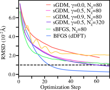
Figure 1: Comparison of the RMSD along an optimization trajectory for $\mbox{Si}_{216}$ using ew-efsDFT with $N_{\chi}=80$ for various stochastic optimization techniques. The blue and green curves depict the deterministic BFGS results (reference calculation) and sBFGS, respectively. sGDM with $\gamma=0$, sGDM($\gamma=0.5$), and $\gamma=0.9$ are shown in red, magenta, and orange, respectively. For $\gamma=0.5$ we also show results with $N_{\chi}=320$ stochastic orbitals (purple curve).

Typical optimization trajectories for Si₂₁₆ are shown in Fig. 1, where we plot the root-mean-square-distance (RMSD) between the current structure and the equilibrium structure (obtained from using deterministic DFT) as a function of the optimization step. The stochastic results are compared to a deterministic DFT optimization using the BFGS method, which converges monotonically to the optimized structure and requires $\approx 20-30$ steps to reach chemical accuracy (RMSD$\leq 0.01\AA$ - dashed horizontal line). Comparing the different stochastic optimization algorithms, we find, as expected, that the sGD (sGDM with $\gamma=0$) requires over $60$ steps to reach and RMSD of $\approx 0.02\AA$. The slow descent rate of sGD results from the ill-conditioned Hessian matrix of a large solid state system. The convergence is much faster when $\gamma$ takes a finite value (sGDM with $\gamma=0.5$), however, as $\gamma\rightarrow 1$ (sGDM with $\gamma=0.9$) the optimization trajectory does not follow the descent direction and the RMSD oscillates with the optimization step. Furthermore, the RMSD of the optimized structure is rather large ($\approx 0.02\AA$) compared to the other stochastic approaches shown, with the same level of statistical noise.

In order to better understand the role of the noise and on the optimized structure, we assumed that the force covariance matrix, $\mathbf{\Sigma}$, is diagonal. In this case, Eqs .(8a) and (8b) are simply a discretized version of the following Langevin equation:

$$m\ddot{{\bf R}}=-m\eta\dot{{\bf R}}+\langle{\bf F}\rangle+\sqrt{2k_{\mathrm{B}}T_{\mathrm{eff}}m\eta}~{}\mathbf{W}(t),$$ (10)

where the mass $m=\Delta x$, the friction $\eta=(1-\gamma)/\Delta x$, and $\mathbf{W}(t)$ is white noise (see supplementary information for more information). In the above equation, $k_{\mathrm{B}}$ is the Boltzmann constant and $T_{\mathrm{eff}}$ is an effective temperature:

$$T_{\mathrm{eff}}=\frac{\Delta x\sigma^{2}}{2k_{\mathrm{B}}(1-\gamma)}\;\;\ldotp$$ (11)

The invariant probability distribution of Eq. (10) is the Boltzmann distribution:

$$P({\bf R})=\frac{1}{Q}e^{-\frac{V({\bf R})}{k_{\mathrm{B}}T_{\mathrm{eff}}}}$$ (12)

where $Q$ is the partition function and $V({\bf R})$ is the potential energy function that depends on the nuclei positions. From Eqs. (11) and (12) we can conclude (a) The effective temperature is linearly dependent on the step size, $\Delta x$ and (b) The effective temperature is inversely proportional to $\gamma$. We note in passing that there are different variants of sGD with adaptive step size like RMSProp [42] and Adam [43], which are usually important in the averaging stage.

The optimization results of sGDM with $N_{\chi}=80$ and $N_{\chi}=320$ suggest that reducing noise in sDFT is not helpful in the early stage of the optimization. The magnitude of the force, $\langle{\bf F}\rangle$, is much larger then $\sigma$ in the descent stage and thus, increasing $\sigma$ does not change the descent direction significantly. Therefore, one can use a small number of stochastic orbitals at the descent stage and increase the number of stochastic orbitals as the optimization progresses to the averaging stage. Comparing the results in Fig. 1 at early and later stages of the optimization for $N_{\chi}=80$ and $N_{\chi}=320$ stochastic orbitals, clearly show the advantage of using more stochastic orbitals at the averaging stage. Increasing the number of stochastic orbitals along the optimization trajectory (“on the fly”) is analogous to increasing the batch sizes in sGD optimizations for machine learning.[56]

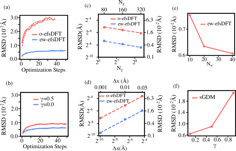
Figure 2: (a) Reverse optimizations trajectories using sGD for o-efsDFT (red solid line) and ew-efsDFT (blue solid line). Dashed lines are fits to Eq. (14). (b) Reverse optimization trajectories comparing sGD (solid blue line) and sGDM (solid red line) with $\gamma=0.5$. Dashed lines are fits to Eq. (14). (c) A log-log plot of the variance in the nuclei positions, RMSD vs. the number of stochastic orbitals, $N_{\chi}$, using with o-efsDFT (red symbols) and ew-efsDFT (blue symbols). Power law fits ($\mathrm{RMSD}\propto N_{\chi}^{-\alpha}$) are shown by the dashed lines, with exponents given by $\alpha=0.48$ and $\alpha=0.51$, respectively. (d) A log-log plot of the variance in the nuclei positions, RMSD vs. the optimization step size, $\Delta x$, using with o-efsDFT (red symbols) and ew-efsDFT (blue symbols). Power law fits ($\mathrm{RMSD}\propto\Delta x^{\eta}$) are shown by the dashed lines, with exponents given by $\eta=0.62$ for both calculations. (e) The optimized RMSD vs. the number of windows used in ew-efsDFT, $N_{w}$. (f) The RMSD of optimized structure vs. $\gamma$ using ew-efsDFT.

To better understand the behavior of the different optimization approaches in the averaging stage, we initiated optimization trajectories from the equilibrium structure obtained by deterministic DFT and analyzed the behavior of the RMSD for different noise levels, friction, and step sizes. The results are summarized in Fig. 2. Two such optimization trajectories are shown in Fig. 2(a) for o-efsDFT (red curve) and ew-efsDFT (blue curve) using sGDM with $\gamma=0$ and $\Delta x=0.01$. The RMSD increases from its optimal value of $0$, approaching a plateau at long times, resulting from the noisy forces in both sDFT methods. Since the fluctuations of the forces on the nuclei in o-efsDFT are larger than those in ew-efsDFT (as a result of using energy windowing,[35]) the plateau value of the RMSD is significantly larger, and the approach to the plateau is slower in the former.

Both optimization trajectories fluctuate about the optimized structure, and thus, the forces on the nuclei can be approximated by Hooke’s law. In this limit, a reversed optimization trajectory for sGDM is equivalent to a discretized version of an Ornstein-Uhlenbeck (O-U) process (see SI for more information) for a small $\Delta x$:

$$\dot{x}=-kx+\sigma W(t).$$ (13)

In the above, $k$ is the force constant and $W$ is the random white noise. The variance of $x$ at time $t$ for the above is given by:[57]

$$\mathrm{Var}(x(t))\approx\frac{\Delta x\sigma^{2}}{2k(1-\gamma)}\left(1-e^{-2kt/(1-\gamma)}\right)$$ (14)

Inspired by Eq. (14), we fitted the RMSD curves shown in Fig. 2 panels (a) and (b) to Eq. (14) (dashed curves), with $\sigma$ and $k$ used as free parameters. The fits seem to describe the numerical data quite accurately. The above expression suggests that increasing $\gamma$ should result in a larger RMSD plateau and fast converges, which is indeed the numerical case shown in Fig. 2(b), reconfirming Eq. (11).

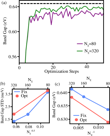
Figure 3: (a) The fundamental band gap along an optimization trajectory using ew-efsDFT and sGDM with $\gamma=0.4$. Purple and green curves correspond to $N_{\chi}=80$ and $N_{\chi}=320$, respectively. The black dashed line is the band gap calculated by deterministic DFT for the optimized structure. (b) and (c) show the standard deviation of the band gap and the average band gap calculated during the averaging stage of the optimization (red symbols) and for the equilibrium structure (blue symbols) vs. the inverse number of stochastic orbitals.

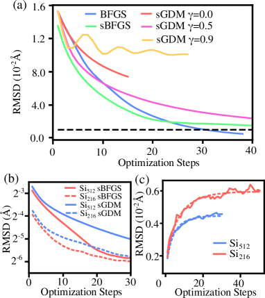
Figure 4: (a) Same as Fig. 1 for $\mbox{Si}_{512}$. (b) Comparison of RMSD along an optimization trajectory for Si₂₁₆ (dashed lines) and Si₅₁₂ (solid lines). (c) Same as panel (b) for a reverse optimization.

In Fig. 2 panels (c) and (d) we show the variance in the position of the nuclei (RMSD) as a function of the number of stochastic orbitals and the step size, respectively. We find that $\mathrm{RMSD}\propto N_{\chi}^{-0.5}$ and $\mathrm{RMSD}\propto\Delta x^{0.62}$, in close agreement with the expected statistical values. Panels (c) and (d) of Fig. 2 also show that ew-efsDFT leads to a much better-optimized structure compared to o-efsDFT regardless of parameters used in optimizations. However, increasing $N_{w}$ above $20$ in ew-efsDFT only marginally improves the results, as shown in Fig. 2(e). Finally, in Fig.(2)(f) we show the RMSD as a function of $\gamma$, which is a non-linear function of $\gamma$, consistent with Eq. (14). The numerical ratios of RMSD with $\gamma=0.1$, $0.5$ and $0.9$ are $1:1.41:3.28$ in good agreement with the predicted values based on Eq. (14) ($1:1.41:3.0$).

In Fig. 3(a) we plot the fundamental band gap along an optimization trajectory for $N_{\chi}=80$ and $N_{\chi}=320$ stochastic orbitals. The gaps were calculated by diagonalizing the KS Hamiltonian for each configuration along the trajectory. The results are shown for sGDM with $\gamma=0.5$ using ew-efsDFT. In the descent stage, the gap changes markedly, while in the averaging stage, it fluctuates about an average value, approaching the deterministic gap (black curve) as $N_{\chi}$ increases. The fluctuations in the band gap result from fluctuations in the structure and the electron density. The latter’s effect is summarized in Fig. 3(b), where we plots the standard deviation in the band gap for the equilibrium geometry as a function of the number of stochastic orbitals. The standard deviation of the band gap follows the expected $N_{\chi}^{-1/2}$, consistent with the central limit theorem, with values on the order of several meVs. We also find that sDFT always underestimates the gaps, as shown in Fig. 3(a) for two values of $N_{\chi}$. As shown in Fig. 3(d), the systematic error is slightly larger for the optimized structures compared to sDFT calculation of the equilibrium structure with a 5 meV difference. The systematic error scales linearly as $N_{\chi}^{-1}$ which is consistent with previous studies.[58]

Finally, we tested the stochastic optimization methods for Si₅₁₂ using ew-efsDFT. The results are shown in Fig. 4. Similar to the case of Si₂₁₆ discussed above, BFGS provides the fastest convergence of the RMSD, but it takes $\approx 30$ optimization steps to achieve chemical accuracy compared $\approx 25$ optimization steps for Si₂₁₆. This slower convergence of the deterministic approach is also observed for all stochastic optimization methods used in this work. However, the conclusion drawn for Si₂₁₆ also holds for the more extensive system; specifically, the optimal value suggested for $\gamma$ in sGDM. In Fig. 4(b) we show a more direct comparison of the optimization trajectories using sBFGS and sGDM for two system sizes. We note that the RMSD for both system sizes are parallel in the descent stage for both stochastic optimization methods, indicating that the optimization efficiencies of both sBFGS and sGDM are comparable and are independent of the system size. Fig. 4(c) shows reverse optimization trajectories for the two system sizes, indicating that the accuracy in determining the optimized structure is somewhat better for the larger systems, likely due to self-averaging. This effect, in fact, suggests that one can reduce the number of stochastic orbitals used as the system size increases and achieve sub-linear scaling for the same level of accuracy.

VI Conclusion

In this work, we assessed the efficiency and accuracy of obtaining the ground state structure of extended systems by combining the linear scaling sDFT to compute the forces on the nuclei with stochastic optimization techniques, such as the stochastic gradient descent with momentum and the stochastic BFGS approach. Typical optimization trajectories can be divided into a descent step where the forces on the nuclei are more significant than the fluctuations, followed by an averaging stage. We analyzed the role of noise, controlled by the number of stochastic orbitals, the number of windows, and the size of the fragments, in sDFT on the optimization trajectories for two different system sizes. We showed that both optimization methods could efficiently determine the optimal structure of extended systems with chemical accuracy by tuning the optimization parameters on small systems.

Supplementary Material

The asympototic behaviors of a reversed optimization trajectory with Langevin equation are provided in the supplementary material.

DATA AVAILABILITY

All data that presented in this study are available from the corresponding author upon reasonable request.

References

- Hohenberg and Kohn [1964] P. Hohenberg and W. Kohn, Phys. Rev. 136, B864 (1964).
- Kohn and Sham [1965] W. Kohn and L. J. Sham, Phys. Rev. 140, A1133 (1965).
- Parr and Yang [1995] R. G. Parr and W. Yang, Annu. Rev. Phys. Chem. 46, 701 (1995).
- Neugebauer and Hickel [2013] J. Neugebauer and T. Hickel, WIREs Computational Molecular Science 3, 438 (2013).
- Seeger and Izgorodina [2020] Z. L. Seeger and E. I. Izgorodina, Journal of Chemical Theory and Computation 16, 6735 (2020).
- Bálint and Jäntschi [2021] D. Bálint and L. Jäntschi, Mathematics 9 (2021).
- Liou et al. [2021] K.-H. Liou, A. Biller, L. Kronik, and J. R. Chelikowsky, J. Chem. Theory Comput. 17, 4039 (2021).
- Packwood et al. [2016] D. Packwood, J. Kermode, L. Mones, N. Bernstein, J. Woolley, N. Gould, C. Ortner, and G. Csányi, J. Chem. Phys. 144, 164109 (2016).
- Mauri, Galli, and Car [1993] F. Mauri, G. Galli, and R. Car, Phys. Rev. B 47, 9973 (1993).
- Ordejón et al. [1993] P. Ordejón, D. A. Drabold, M. P. Grumbach, and R. M. Martin, Phys. Rev. B 48, 14646 (1993).
- Goedecker [1995] S. Goedecker, J. Comput. Phys. 118, 261 (1995).
- Hernández and Gillan [1995] E. Hernández and M. J. Gillan, Phys. Rev. B 51, 10157 (1995).
- Kohn [1996] W. Kohn, Phys. Rev. Lett. 76, 3168 (1996).
- Palser and Manolopoulos [1998] A. H. R. Palser and D. E. Manolopoulos, Phys. Rev. B 58, 12704 (1998).
- Yang [1991] W. Yang, Phys. Rev. Lett. 66, 1438 (1991).
- Cortona [1991] P. Cortona, Phys. Rev. B 44, 8454 (1991).
- Zhu, Pan, and Yang [1996] T. Zhu, W. Pan, and W. Yang, Phys. Rev. B 53, 12713 (1996).
- Baer and Head-Gordon [1997] R. Baer and M. Head-Gordon, Phys. Rev. Lett. 79, 3962 (1997).
- Luo et al. [2020] Z. Luo, X. Qin, L. Wan, W. Hu, and J. Yang, Front. Chem. 8 (2020), 10.3389/fchem.2020.589910.
- Skylaris et al. [2005] C.-K. Skylaris, P. D. Haynes, A. A. Mostofi, and M. C. Payne, J. Chem. Phys. 122, 084119 (2005).
- Todorović et al. [2013] M. Todorović, D. R. Bowler, M. J. Gillan, and T. Miyazaki, J. R. Soc. Interface 10, 20130547 (2013).
- Nakata et al. [2020] A. Nakata, J. S. Baker, S. Y. Mujahed, J. T. L. Poulton, S. Arapan, J. Lin, Z. Raza, S. Yadav, L. Truflandier, T. Miyazaki, and D. R. Bowler, J. Chem. Phys. 152, 164112 (2020).
- Aarons et al. [2016] J. Aarons, M. Sarwar, D. Thompsett, and C.-K. Skylaris, J. Chem. Phys. 145, 220901 (2016).
- Ruiz-Serrano and Skylaris [2013] A. Ruiz-Serrano and C.-K. Skylaris, J. Chem. Phys. 139, 054107 (2013).
- Mohr et al. [2018] S. Mohr, M. Eixarch, M. Amsler, M. J. Mantsinen, and L. Genovese, Nucl. Mater. Energy 15, 64 (2018).
- Yang and Lee [1995] W. Yang and T. Lee, J. Chem. Phys. 103, 5674 (1995).
- Götz, Beyhan, and Visscher [2009] A. W. Götz, S. M. Beyhan, and L. Visscher, J. Chem. Theory Comput. 5, 3161 (2009).
- Wesolowski, Shedge, and Zhou [2015] T. A. Wesolowski, S. Shedge, and X. Zhou, Chem. Rev. 115, 5891 (2015).
- Goodpaster, Barnes, and Miller [2011] J. D. Goodpaster, T. A. Barnes, and T. F. Miller, J. Chem. Phys. 134, 164108 (2011).
- Huang and Carter [2011] C. Huang and E. A. Carter, J. Chem. Phys. 135, 194104 (2011).
- Baer, Neuhauser, and Rabani [2013] R. Baer, D. Neuhauser, and E. Rabani, Phys. Rev. Lett. 111, 106402 (2013).
- Neuhauser, Baer, and Rabani [2014] D. Neuhauser, R. Baer, and E. Rabani, J. Chem. Phys. 141, 041102 (2014).
- Chen et al. [2019a] M. Chen, R. Baer, D. Neuhauser, and E. Rabani, J. Chem. Phys. 150, 034106 (2019a).
- Chen et al. [2019b] M. Chen, R. Baer, D. Neuhauser, and E. Rabani, J. Chem. Phys. 151, 114116 (2019b).
- Chen et al. [2021] M. Chen, R. Baer, D. Neuhauser, and E. Rabani, J. Chem. Phys. 154, 204108 (2021).
- Arnon et al. [2017] E. Arnon, E. Rabani, D. Neuhauser, and R. Baer, J. Chem. Phys. 146, 224111 (2017).
- Arnon et al. [2020] E. Arnon, E. Rabani, D. Neuhauser, and R. Baer, J. Chem. Phys. 152, 161103 (2020).
- Robbins and Monro [1951] H. Robbins and S. Monro, Ann. Math. Stat. 22, 400 (1951).
- Rumelhart, Hinton, and Williams [1986] D. E. Rumelhart, G. E. Hinton, and R. J. Williams, Nature 323, 533 (1986).
- Polyak and Juditsky [1992] B. T. Polyak and A. B. Juditsky, SIAM J. Control Optim. 30, 838 (1992).
- Duchi, Hazan, and Singer [2011] J. Duchi, E. Hazan, and Y. Singer, J. Mach. Learn. Res. 12, 2121 (2011).
- Tieleman, Hinton et al. [2012] T. Tieleman, G. Hinton, et al., COURSERA: Neural networks for machine learning 4, 26 (2012).
- Kingma and Ba [2014] D. P. Kingma and J. Ba, arXiv , 1412:6980 (2014).
- Schraudolph, Yu, and Günter [2007] N. N. Schraudolph, J. Yu, and S. Günter, in Proceedings of the Eleventh International Conference on Artificial Intelligence and Statistics, Proceedings of Machine Learning Research, Vol. 2 (PMLR, San Juan, Puerto Rico, 2007) pp. 436–443.
- Johnson and Zhang [2013] R. Johnson and T. Zhang, in Advances in Neural Information Processing Systems, Vol. 26 (Curran Associates, Inc., 2013).
- Baer, Neuhauser, and Rabani [2022] R. Baer, D. Neuhauser, and E. Rabani, Annu. Rev. Phys. Chem. 73, 255 (2022).
- Kosloff [1988] R. Kosloff, J. Phys. Chem. 92, 2087 (1988).
- Kosloff [1994] R. Kosloff, Annu. Rev. Phys. Chem. 45, 145 (1994).
- Lan [2020] G. Lan, First-order and Stochastic Optimization Methods for Machine Learning, Springer Series in the Data Sciences (Springer International Publishing, 2020).
- Jin and He [2020] R. Jin and X. He, in 2020 IEEE 16th International Conference on Control & Automation (ICCA) (2020) pp. 779–784.
- Nemirovski et al. [2009] A. Nemirovski, A. Juditsky, G. Lan, and A. Shapiro, SIAM J. Opt. 19, 1574 (2009).
- Skylaris and Haynes [2007] C.-K. Skylaris and P. D. Haynes, J. Chem. Phys. 127, 164712 (2007).
- Troullier and Martins [1991] N. Troullier and J. L. Martins, Phys. Rev. B 43, 1993 (1991).
- Kleinman and Bylander [1982] L. Kleinman and D. M. Bylander, Phys. Rev. Lett. 48, 1425 (1982).
- King-Smith, Payne, and Lin [1991] R. D. King-Smith, M. C. Payne, and J. S. Lin, Phys. Rev. B 44, 13063 (1991).
- De et al. [2017] S. De, A. Yadav, D. Jacobs, and T. Goldstein, in Proceedings of the 20th International Conference on Artificial Intelligence and Statistics, Proceedings of Machine Learning Research, Vol. 54 (PMLR, 2017) pp. 1504–1513.
- Varadhan [2007] S. Varadhan, Stochastic Processes, Courant lecture notes in mathematics (Courant Institute of Mathematical Sciences, 2007).
- Fabian et al. [2019] M. D. Fabian, B. Shpiro, E. Rabani, D. Neuhauser, and R. Baer, WIREs Comput. Mol. Sci. 9, e1412 (2019).