CUTS: A Framework for Multigranular
Unsupervised Medical Image Segmentation
 

Abstract

Segmenting medical images is critical to facilitating both patient diagnoses and quantitative research. A major limiting factor is the lack of labeled data, as obtaining expert annotations for each new set of imaging data or task can be expensive, labor intensive, and inconsistent among annotators. To address this, we present CUTS (Contrastive and Unsupervised Training for multi-granular medical image Segmentation), a fully unsupervised deep learning framework for medical image segmentation to better utilize the vast majority of imaging data that are not labeled or annotated. CUTS works by leveraging a novel two-stage approach. First, it produces an image-specific embedding map via intra-image contrastive loss and a local patch reconstruction objective. Second, these embeddings are partitioned at dynamic levels of granularity that correspond to the data topology. Ultimately, CUTS yields a series of coarse-to-fine-grained segmentations that highlight image features at various scales. We apply CUTS to retinal fundus images and two types of brain MRI images in order to delineate structures and patterns at different scales, providing distinct information relevant for clinicians. When evaluated against predefined anatomical masks at a given granularity, CUTS demonstrates improvements ranging from 10% to 200% on dice coefficient and Hausdorff distance compared to existing unsupervised methods. Further, CUTS shows performance on par with the latest Segment Anything Model which was pre-trained in a supervised fashion on 11 million images and 1.1 billion masks. In summary, with CUTS we demonstrate that medical image segmentation can be effectively solved without relying on large, labeled datasets or vast computational resources.

1 Introduction

Medical image segmentation plays an increasingly crucial role in both research and clinical settings in a wide array of imaging modalities including microscopy, X-ray, ultrasound, optical coherence tomography (OCT), computed tomography (CT), magnetic resonance imaging (MRI), positron emission tomography (PET), and others [1]. With high-quality image segmentation, clinicians can more easily diagnose and monitor the progression of diseases to improve patient care. Traditional medical image segmentation methods rely on hand-crafted features [2, 3, 4, 5, 6, 7] or predefined atlases [8, 9, 10]. These methods are gradually being replaced by deep learning [11, 12, 13, 14] as supervised neural networks demonstrate superior performance than feature-based methods and less overhead than atlas-based methods. Although supervised neural networks have been widely successful in image segmentation in recent years, there are several issues in applying them to medical images, particularly in order to make clinical inferences. First, these networks depend on expert annotations, so they require a large number of labels to adequately cover the data variance to produce reliable segmentations [12]. Second, supervised networks trained on one set of annotated images can fail to generalize to similar images collected in very slightly different contexts, such as in different patient populations or on different devices [15]. Third, the desired segmentation granularity may vary across use cases even if the exact same image is concerned — for example, localizing a brain tumor would require a finer segmentation compared to measuring the brain volume — yet this need is not easily accommodated by supervised approaches without updating the labels.

To address these issues, we propose to automatically segment medical images using an entirely unsupervised framework that combines recent advances in representation learning with advances in data geometry and topology. An unsupervised approach circumvents the need for costly expert annotations and alleviates the cross-domain generalization problem. More importantly, we also design our approach to produce multigranular segmentations, which can potentially target multiple regions of interest without supervision.

Our framework, which we denote Contrastive and Unsupervised Training for multigranular medical image Segmentation (CUTS), was named as an homage to the renowned painter Henri Matisse, who famously used a “cut-up” method he called “drawing with scissors” to assemble an image based on patches of material from different sources. Our technique is in essence the reverse of this process, as we start with the initial image and use unsupervised machine learning to segment the initial figure into a collection of relatively homogeneous patches using data coarse graining in a learned latent space. Although it may seem trivial to identify the different pieces of paper cut up by scissors, segmentation of medical images is more challenging as the boundaries between biological structures, such as between healthy and pathological tissues, are not always sharp and clean.

CUTS is designed as a fully unsupervised segmentation pipeline. The images are processed in units of pixel-centered patches, which consists of a fixed-size crop of image centered on an image pixel. A convolutional encoder is then trained on these pixel-centered patches with both intra-image contrastive learning and local patch reconstruction as optimization objectives. We note that contrastive patches should come from the domain of the medical image itself to create a meaningful pixel embedding. Thus, we find suitable contrastive patches within each image itself using an image similarity metric. Subsequently, the learned embedding space serves as a stronger feature-rich foundation for a multiscale, topology-based data coarse graining method called diffusion condensation that produces multigranular segmentations.

Our main contributions include:

• CUTS, a novel unsupervised framework with a two-stage approach: it first produces an image-specific pixel-centered patch embedding via a convolutional encoder, and subsequently diffusion condensation coarse-grains these patches into clusters at various levels of granularity. At each granularity, the cluster assignments can be mapped one-to-one back to the image space as segmentations.

• (Specific to the first stage) A novel optimization objective that combines intra-image contrastive learning with local patch reconstruction to help the convolutional encoder learn an expressive embedding space.

• (Specific to the second stage) A multiscale cluster assignment approach that utilizes diffusion condensation, which provides clinicians with labels at multiple levels of segmentation granularities, potentially highlighting clinically relevant regions at various scales.

The remainder of this paper is organized as follows. First, we discuss related work in the field. With this provided context, we then introduce our framework detailing the neural network architecture, optimization objective, and multiscale segmentation. Finally, we apply our framework on a series of medical image datasets consisting of retinal fundus images and brain MRI images We evaluate the performance of CUTS through qualitative and quantitative metrics and compare to several baselines including other unsupervised approaches and supervised approaches.

2 Related work

2.1 Traditional methods for medical image segmentation

Traditional image segmentation methods generally fall into two categories. The first category relies on hand-crafted image features, such as line/edge detection [2], graph cuts [3, 7], active contours [4], watershed [5, 6], level-set [16], and feature clustering [17]. The methods in this category are simple to execute, but they usually struggle with images with more complicated colors and textures. The second category utilizes a precomputed and annotated atlas to propagate prior knowledge, by warping a predefined set of labels onto new images through image registration [8, 9, 10]. These methods require building and annotating an atlas for each image dataset – a time-consuming process that may sometimes be impractical.

2.2 Supervised learning for medical image segmentation

Supervised deep learning has outperformed traditional methods in segmenting medical images in the past decade [13]. In supervised deep learning, a neural network learns to perform a designated task through a data-driven parameter optimization process [11]. In medical image segmentation, the most well-known method is U-Net [18], followed by a proliferation of variants with skip connections, attention mechanisms, etc. [19, 20, 21, 22, 23, 24]. They are all supervised learning methods and thereby require an abundance of expert annotations.

2.3 Towards unsupervised learning

With a growing emphasis on avoiding reliance on human expert annotations, researchers have been exploring unsupervised learning approaches for medical image segmentation. Many works focused on training with fewer data [25, 26, 27, 28, 29]. SSL-ALPNet [30] proposed to directly learn from pseudo-labels generated from Felzenswalb segmentation [7], thus categorizing it as an unsupervised learning method despite a supervised learning approach. DCGN [31] used a constrained Gaussian mixture model to cluster pixel representations in histopathology images. It assumes that different tissue types correspond to different colors, which is not necessarily true in many other medical image modalities.

Atlas-based unsupervised learning is another promising direction. Compared to their traditional counterparts [8, 9, 10], the versions empowered by deep learning [32, 33] have improved results. When the domain gap is small, they can be highly effective; otherwise, these methods could fail similarly. Given their requirement for spatial registration, they are more suitable for clearly defined structures that show little variation among individuals and thus are less applicable to image domains with greater variability.

2.4 Contrastive learning

Contrastive learning [34] was proposed as a generic self-supervised method to address the issue of limited annotations. Conceptually, it allows neural networks to learn meaningful representations in the embedding space by encouraging similar image pairs to be embedded closer to each other and vice versa. After a meaningful embedding space is trained, additional layers can be attached and fine-tuned for downstream tasks. In particular, commonly used contrastive learning methods such as SimCLR [34], SwaV [35], MoCo [36], BYOL [37], BarlowTwins [38] and SimSiam [39] focus on extracting image-level representations with an inter-image contrastive objective. These image-level contrastive learning methods yield no information about intra-image features and are therefore unsuitable for tasks that require closer scrutiny within the same image, such as image segmentation. In an attempt to adapt contrastive learning to tackle the image segmentation task, [40] proposed learning image and patch representations through global and local contrastive training. In [41], the authors used a similar approach, although they coined different terminologies. Both methods include a supervised fine-tuning stage after contrastive pre-training, which still depends on labels.

2.5 Unsupervised image segmentation with contrastive learning

Two leading unsupervised image segmentation methods, DFC [42] and STEGO [43], both utilize contrastive learning concepts. STEGO learns feature relationships between an image and itself, its $k$ most similar images, and dissimilar images. Although STEGO can be trained without labels, it relies on pre-trained vision backbones for knowledge distillation, which is not a requirement in our method. DFC is by far the most similar to our approach, yet with two key differences. First, DFC contrasts on pixels, while we operate on pixel-centered patches. Pixel-centered patches contain significantly richer semantic and textural information than pixels. Second, we achieve segmentation through a topological multiscale coarse-graining method that produces many segmentation maps at various granularities rather than a single segmentation map.

2.6 Segment Anything Model (SAM)

Segment Anything Model (SAM) [44] recently introduced a general-purpose segmentation tool pre-trained on a gigantic dataset with 11 million images and 1.1 billion masks. As previous researchers have shown [45], SAM offers an alternative solution to label-free medical image segmentation through an interface called “zero-shot transfer”, where a single point is provided as a prompt which is deciphered by a prompt encoder and sent to a mask model to produce a segmentation mask.

Strictly speaking, SAM is not an unsupervised learning method. As a result, SAM still faces the cross-domain generalization problem as previously mentioned, while their brute-force solution is to cover the entire data distribution with the huge training set. Despite its non-unsupervised nature, we decided to include it for comparison, since it is arguably the latest state-of-the-art segmentation framework.

3 Methods

Figure 1: The CUTS Framework. (A) Overview. (B) The convolutional encoder maps pixel-centered patches into a structured and expressive latent embedding space. CUTS combines two unsupervised objectives — a contrastive loss and an autoencoder-inspired reconstruction loss — to jointly guide the learning of the embedding space. (C) A proximity check and a structural similarity check are used to find similar and dissimilar patches within each image for contrastive learning. (D) Diffusion condensation coarse grains embedding vectors into clusters at multiple granularities and performs a series of coarse-to-fine segmentations. (E) During the diffusion condensation process, we can take the embeddings at any iteration and generate the image segmentation for that granularity by mapping the cluster assignments back to the image space. Multiscale PHATE (MS-PHATE) [46] is used for visualization.

In this section, we detail our framework “Contrastive and Unsupervised Training for multi-granular medical image Segmentation” (CUTS). On a high level, CUTS consists of two sequential stages, as illustrated in Fig. 1(A). In the first stage, it encodes each pixel in the image along with the local neighborhood around it, denoted as a “pixel-centered patch”, into a high-dimensional latent space by jointly optimizing contrastive learning and autoencoding objectives (Fig. 1(B)). Unlike most contrastive learning methods that learn from augmented versions of full images, CUTS learns from regions within the same image curated through a pipeline utilizing spatial proximity and structural similarity (SSIM) (Fig. 1(C)). Such modification allows the network to learn local, intra-image features instead of emphasizing invariance over known image transformations or noise models. This is especially critical for medical images, since they are globally homogeneous (i.e., images from different participants capture the same body part and are filmed with similar or even identical imaging parameters) yet locally heterogeneous (i.e., clinically important knowledge are drawn from nuances in structures or textures within small areas of the image). In the second stage, these embedding vectors are coarse-grained to many levels of granularity, and segmentation is performed by assigning unique labels to pixels that correspond to unique clusters arising from a particular level of granularity (Fig. 1(D-E)).

3.1 Learning an embedding space for pixel-centered patches

CUTS uses a convolutional neural network (ConvNet) as an encoder to map the pixel-centered patches from the image space to a latent embedding space. The architecture is further described in supplementary materials section A. During the training of the encoder, two objectives are jointly optimized: a contrastive loss and a local patch reconstruction loss.

3.1.1 Contrastive loss

Contrastive loss operates on the embedding space and pulls together the representations of similar pixel-centered patches and pushes apart dissimilar pairs. Pairs of similar pixel-centered patches are referred to as “positive examples” and dissimilar ones “negative examples”. Formally, for any anchor patch $\mathcal{P}_{ij}\in\mathbb{R}^{p\times p\times c}$ centered at image-space coordinates $(i,j)$, we sample a set of positive patches $\{\mathcal{P}^{+}_{ij}\}$ and negative examples $\{\mathcal{P}^{-}_{ij}\}$. Let $f$ denote the convolutional encoder. The anchor embedding $z_{ij}=f(\mathcal{P}_{ij})$, the set of positive embeddings $\Omega^{+}:=\{z^{+}_{ij}\}=\{f(\mathcal{P}^{+}_{ij})\}$, and the set of negative embeddings $\Omega^{-}:=\{z^{-}_{ij}\}=\{f(\mathcal{P}^{-}_{ij})\}$. After projecting the patches to the latent embedding space, we can perform contrastive learning on their respective embedding vectors $z^{+}_{ij}$ and $z^{-}_{ij}$.

To ensure our method is completely unsupervised, we mine these positive and negative examples using a combination of a simple proximity heuristic and an image similarity metric. We scan the nearby patches within a local neighborhood of the anchor patch, and use structural similarity index (SSIM) [47] to screen for patches that are similar enough to the anchor patch. If they meet or exceed a threshold of similarity set as a hyperparameter for our model, then they are used as a positive example. Patches far away from the anchor or nearby patches that fail the structural similarity check are all considered negative examples. In this way, we can generate positive and negative pairs for our contrastive loss without needing supervised labels in any way and build invariances into our embedding. In practice, we can directly use the positive examples from a different anchor patch as the negative example of the current anchor patch, as suggested in [34]. This simplification can speed up the mining processes by a factor of 2.

The contrastive loss is defined as:

$$l_{contrastive}=-\log\hskip 4.0pt\frac{\sum_{z^{+}_{ij}\in{\Omega}^{+}}e^{sim(z_{ij},z^{+}_{ij})/\tau}}{\sum_{z^{-}_{ij}\in{\Omega}^{-}}e^{sim(z_{ij},z^{-}_{ij})/\tau}}$$

Note that minimizing this loss will encourage the network to embed the positive set $\Omega^{+}$ close to the anchor, with closeness scaled by the distance between the negative set $\Omega^{-}$ and the anchor. In this way, this loss accomplishes the goal of encouraging similar pairs to be embedded more closely and dissimilar pairs more distantly. $sim(\cdot)$ denotes cosine similarity. The temperature parameter $\tau$ controls how the distances used in the contrastive loss are scaled. We fixed $\tau$ at $0.5$ following the suggestion in [34].

3.1.2 Local patch reconstruction loss

In addition to the contrastive loss, we ensure our embedding of each pixel-centered patch retains information about the patch around it by utilizing a reconstruction loss. We made this design choice as we would like the embedding vector for a pixel-centered patch to retain sufficient information about its original intensities and structures in the image space, such that it is possible to reconstruct the patch directly from the embedding vector.

For an embedding $z_{ij}\in\mathbb{R}^{d}$, the patch reconstruction loss is:

$$l_{recon}=||\mathcal{P}_{ij}-f_{recon}(z_{ij})||_{2}^{2}$$

where $f_{recon}(\cdot):\mathbb{R}^{d}\rightarrow\mathbb{R}^{p\times p\times c}$ is a patch reconstruction module jointly optimized with the convolutional encoder during training. In implementation, $f_{recon}(\cdot)$ can be as simple as a single-layered fully connected network. By enforcing reconstruction of the patch around the corresponding pixel from each embedding vector, we ensure that the embedding space is an expressive representation that retains sufficient information of the local neighborhood.

3.1.3 Final objective function

The final objective function for our network is the sum of the contrastive loss and the reconstruction loss, balanced with a weighting coefficient $\lambda\in[0,1]$ controlling the relative magnitude:

$$loss=\lambda\cdot l_{contrastive}+(1-\lambda)\cdot l_{recon}$$

We set $\lambda=0.01$ in all our experiments. The rationale can be found in supplementary materials section B.

3.2 Coarse-graining for multi-scale segmentation

Once we have trained our convolutional encoder and therefore a latent embedding space, each pixel-centered patch in the input image is respectively mapped to a vector of dimension $\mathbb{R}^{d}$. Then, image segmentation can be achieved by coarse-graining these embedding vectors.

More formally, for each image patch $\mathcal{P}_{ij}$ centered at coordinates $(i,j)$, the convolutional encoder assigns it an embedding $z_{ij}\in\mathbb{R}^{d}$. For an image with width $W$ and height $H$, we will have a total of $W\times H$ such $d$-dimensional vectors in the embedding space. We can assign them in to $n$ different clusters $\{c_{1},c_{2},...,c_{n}\}$ using a clustering algorithm $cls(\cdot):\mathbb{R}^{d}\rightarrow\mathbb{R}$. With that, we can create a label map $L\in\mathbb{R}^{H\times W}$ where $L_{ij}=cls(z_{ij})$. The label map $L$ will be the end product of CUTS segmentation. Notably, with diffusion condensation, $cls(\cdot)$ effectively changes along the process, and therefore we can generate a rich set of labels $\{L\}$ each of which is a segmentation at a particular scale.

3.2.1 Diffusion condensation for multi-scale coarse-graining

Diffusion condensation [48, 49] is a dynamic process that sweeps through various levels of granularities to identify natural groupings of data. It iteratively condenses data points towards their neighbors through a diffusion process, at a rate defined by the diffusion probability between the points. Unlike most clustering methods, diffusion condensation constructs a full hierarchy of coarse-to-fine granularities where the number of clusters at each granularity is not arbitrarily set but rather inferred from the underlying structure of the data.

Formally, from a data matrix $X^{N\times d}$ with $N$ observations (in our case, $N=W\times H=$ the number of pixels in an image) and $d$ features, we can construct the local affinity among each observation pair $(m,n)\in\{1,...,N\}$ using a Gaussian kernel

$$\mathbf{K}(x_{m},x_{n})=e^{-\frac{||x_{m}-x_{n}||^{2}}{\epsilon}}$$ (1)

$\mathbf{K}$ is a $N\times N$ Gram matrix whose $(m,n)$ entry is denoted $\mathbf{K}(x_{m},x_{n})$ to emphasize the dependency on the data matrix $X$. $X_{m}$ and $x_{j}$ are both of dimension $\mathbb{R}^{d}$. The bandwidth parameter $\epsilon$ controls neighborhood sizes.

Given this affinity matrix $\mathbf{K}$, the diffusion operator is defined as

$$\mathbf{P}=\mathbf{D}^{-1}\mathbf{K}$$ (2)

where $\mathbf{D}$ is the diagonal degree matrix

$$\mathbf{D}(x_{m},x_{m})=\sum_{n}\mathbf{K}(x_{m},x_{n})$$ (3)

The diffusion operator $\mathbf{P}$ defines the single-step transition probabilities for a diffusion process over the data, which can be viewed as a Markovian random walk. To perform multi-step diffusion, one way is to simulate a time-homogeneous diffusion process by raising the diffusion operator to a power of $t$ which leads to $X_{t}=\mathbf{P}^{t}X$ [50]. On the other hand, as shown in [49], we could simulate a time-inhomogeneous diffusion process by iteratively computing the diffusion operator and the data matrix in the following manner.

$$X_{0}\leftarrow X$$

$$\mathbf{for}\hskip 4.0ptt\in[1,...,T]:$$

$$\hskip 20.0pt\mathbf{K}_{t-1}\leftarrow\mathcal{K}(X_{t-1})\hskip 64.0pt\textrm{/* using Eq.~{}\ref{eq:diffusion_K} */}$$

$$\hskip 20.0pt\mathbf{D}_{t-1}\leftarrow\mathcal{D}(\mathbf{K}_{t-1})\hskip 63.0pt\textrm{/* using Eq.~{}\ref{eq:diffusion_D} */}$$ (4)

$$\hskip 20.0pt\mathbf{P}_{t-1}\leftarrow\mathbf{D}_{t-1}^{-1}\mathbf{K}_{t-1}\hskip 60.0pt\textrm{/* using Eq.~{}\ref{eq:diffusion_P} */}$$

$$\hskip 20.0ptX_{t}\leftarrow\mathbf{P}_{t-1}X_{t-1}$$

The process of diffusion condensation can be summarized as the alternation between the following two steps:

1. Computing a time-inhomogeneous diffusion operator from the data at iteration $t$.

2. Applying this operator to the data, moving points towards the local center of gravity, which forms the data in iteration $t+1$.

More details on diffusion condensation can be found in [49]. In this paper, we used the official implementation.

3.2.2 Persistent structures

While the multigranularity nature of diffusion condensation is a favorable trait, in occasions we may desire a single label map. In these situations, we can identify the segments that occur consistently over the series of segmentations. This can be achieved by rank-ordering different segments based on their persistence levels, which is quantified by the number of consecutive diffusion iterations in which the segment stays intact and refrains from being merged into another segment. Finally, we construct a single label map by stacking all segments together, where segments with higher persistence levels override those with lower persistence levels. This constructed label map prioritizing the persistent segments is named persistent structures. The implementation can be found in our public codebase.

3.2.3 From multi-class to binary segmentation

In use cases where the task requests a binary segmentation, we need to convert the multi-class label maps to binary segmentation masks. Similar to [43], we use the ground truth segmentation mask to provide a hint on how to select the foreground for each image. Specifically, we iterate over each foreground pixel in the ground truth mask and find the most frequently associated cluster of the corresponding embedding vector. Finally, we can set all pixels whose embedding equals that cluster label as the foreground and all other pixels as the background.

This process effectively estimates the most probable cluster label if a pixel is randomly selected from the foreground region of the ground truth mask. Therefore, it is relatively objective and unbiased.

4 Results

Figure 2: Qualitative results, evaluated against expert-labeled masks at one single granularity. A sample image from each dataset is displayed for visual comparison. Green curves outline the ground truth labels while blue or red curves outline the various predictions. CUTS provides better segmentation than all competing unsupervised methods: Watershed [5, 6], Felzenswalb [7], SLIC [17], DFC [42] and STEGO [43]. It is on-par with Segment Anything Model (SAM) [44, 45] which utilized large-scale supervised pre-training and is close to the supervised methods UNet [18] and nn-UNet [24]. Notation: “CUTS + $k$-means” represents CUTS with spectral $k$-means clustering; “CUTS + diffusion-P” represents CUTS with diffusion condensation persistent structures.

We prepared three medical image datasets to evaluate our proposed framework (see supplementary materials section C for details). The datasets include: retinal fundus images, brain MRI images without tumors, and brain MRI images with tumors. The datasets are chosen to demonstrate the breadth of applications, as they cover variation in color channels (e.g., RGB versus intensity-only), imaging sequences (e.g., T1-weighted versus T2 FLAIR), and organs of interest (e.g., eye versus brain). These datasets contain images with different characteristics, and the regions of interest are distinguished in different ways. Thus, a model would need to be flexible to capture the meaningful axes of variation in each of these contexts.

We compared the performance of CUTS on the above datasets with several alternative methods. We first compared it with three traditional unsupervised methods: Otsu’s watershed [5], Felzenszwalb [7], and SLIC [17]. We then compared with DFC [42] and STEGO [43], two recent unsupervised models based on deep learning. For each respective experiment, we re-trained DFC, STEGO, and CUTS on the corresponding dataset (images only, no labels) using the official code and then performed segmentation and evaluation. Next, we compared against SAM [44, 45], a popular zero-shot transfer segmentation tool pre-trained on 11 million images with 1.1 billion masks. As described in [45], we provided a center point of the ground truth label as a prompt for segmentation of each image. Lastly, for reference, we benchmarked a random labeler which served as the performance lower-bound and two fully supervised methods, namely UNet [18] and nn-UNet [24], which served as the performance upper-bound for our unsupervised method. A qualitative overview of the segmentation results can be found in Fig. 2, while more extensive results for each dataset are shown in subsequent figures.

For coarse-graining the pixel embeddings, in addition to the diffusion condensation method we propose, we also experimented with a spectral $k$-means clustering [51] alternative which segments at only one granularity level. The choice of $k$ for this clustering is naturally related to the complexity of the image and the desired segmentation, which we empirically set to $k=10$.

When evaluating the results on binary image segmentation, for a fair comparison, we applied the approach described in Section 3.2.3 to all unsupervised methods. This binarization process is similar to how practitioners would choose among machine-generated segments by selecting just a single pixel.

4.1 Geographic atrophy segmentation in retinal fundus images

Our first experiment considers fundus images of retinas, with the goal of identifying and segmenting regions of geographic atrophy (GA). GA is an advanced stage of age-related macular degeneration (AMD) characterized by progressive degeneration of the macula. Automatically segmenting these regions computationally offers the ability to save time and resources for human graders who would have to perform the painstaking task of hand-labeling these images. Moreover, as the boundary of atrophy may not always be clear, two graders may not agree on the segmentation. Quantitative and objective methods offer the opportunity for a more disciplined and rigorous approach to GA region segmentation.

Several challenges exist in the segmentation of GA. For example, the color of GA is similar to the surrounding retina and drusen in many cases. The optic nerve and peripapillary atrophy have similar color to GA. Moreover, the presence of blood vessels and varying degrees of atrophy (varying levels of color differentiation) exemplify the challenges in this task.

Figure 3: Segmenting geographic atrophy in retinal fundus images. (A) Multigranular segmentation (odd rows) captures distinctive patterns at various scales. Multiscale PHATE (even rows) is used to visualize the diffusion condensation process. The results of CUTS + spectral $k$-means clustering (labeled as: $k$-means) and CUTS + diffusion condensation persistent structures (labeled as: diffusion-P) are also shown for reference. (B) Additional sample images in the format of Fig. 2. (C) Quantitative comparisons. An up arrow next to a metric indicates that a higher score is better, and an down arrow otherwise. The methods are displayed in the same order as the legends. CUTS results are highlighted by boxes. Note that SAM, UNet, and nn-UNet are not unsupervised methods.

4.1.1 Qualitative results

As shown in Fig. 3(A), our multi-scale segmentation method provides delineation of retinal structures at various granularities. On the coarser side of the spectrum, our method segments the entire retina from the background. Moving towards the finer scales, anatomical structures such as the optic disc and geographic atrophy regions emerge, providing immediate utilities such as facilitating automatic measurements of their sizes, shapes and locations for planning clinical interventions. On the finer side of the spectrum even smaller structures arise, showing potentials for more delicate tasks such as retinal vessel segmentation. We also observed that our method identifies the central region of atrophy without being perturbed by the presence of blood vessels, despite similarity in color.

For the binarized segmentation results (Fig. 3(B)), the segmentation generated by CUTS accurately picks out the region of atrophy. Despite all the aforementioned challenges in segmenting this dataset, our method successfully segments the GA region. Hence, qualitatively, CUTS is better at delineating atrophy boundaries compared to all other unsupervised methods.

4.1.2 Quantitative results

Quantitative experiments confirmed the accuracy of our segmentation, shown in Fig. 3(C) and Table 1. CUTS created segmentations with higher similarity (SSIM) and lower discrepancies (ERGAS, RMSE) with respect to the ground truth, compared to all the other unsupervised methods. The two most standard metrics for segmentation evaluation, dice coefficient and Hausdorff distance, indicated the same trend as well. As demonstrated in Fig. 3(C) and Table 1, our method produces superior segmentation metrics on this dataset as compared to the other unsupervised methods.

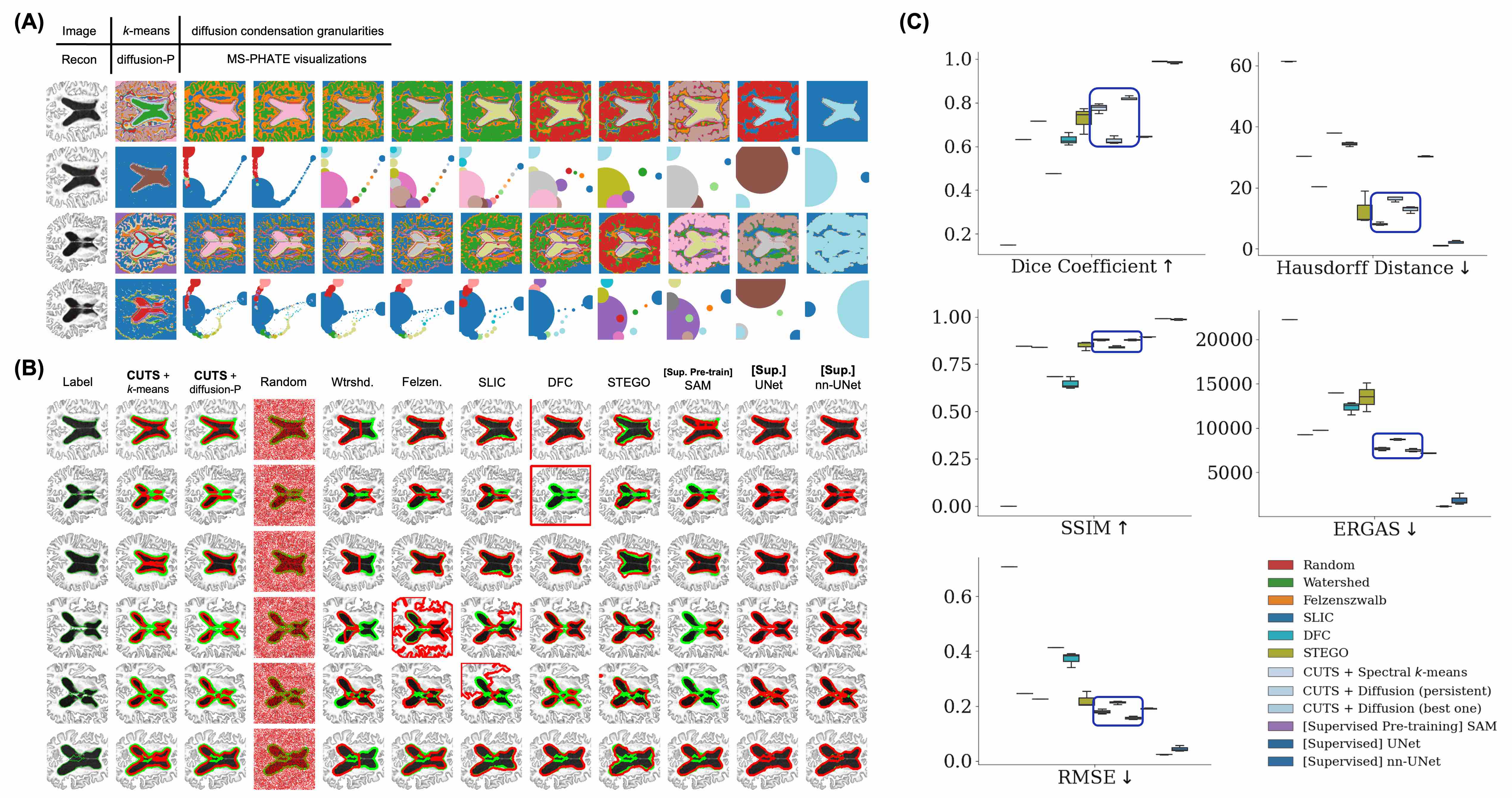
Figure 4: Segmenting ventricles in brain MRI images. (A) Multigranular segmentation (odd rows) captures distinctive patterns at various scales. Multiscale PHATE (even rows) is used to visualize the diffusion condensation process. The results of CUTS + spectral $k$-means clustering (labeled as: $k$-means) and CUTS + diffusion condensation persistent structures (labeled as: diffusion-P) are also shown for reference. (B) Additional sample images in the format of Fig. 2. (C) Quantitative comparisons. An up arrow next to a metric indicates that a higher score is better, and an down arrow otherwise. The methods are displayed in the same order as the legends. CUTS results are highlighted by boxes. Note that SAM, UNet, and nn-UNet are not unsupervised methods.

4.2 Ventricle segmentation in brain MRI images

In our next experiment, we analyzed CUTS performance on a brain magnetic resonance imaging (MRI) dataset obtained from clinical patients at various stages of Alzheimer’s disease. We attempted to automatically segment the brain ventricles on the MRI images of these patients, a task considered clinically important because the volume of the brain ventricles can predict the progression of dementia [52, 53]. The ground truth has been identified from human annotated labels and is used in evaluating performance exclusively as in the other cases.

Challenges in this dataset include an increased complexity in shape and size of the segmentation target. Since the MRI imaging plane (i.e., orientation of image acquisition relative to the brain) can vary between patients, the shape and size of the ventricles can significantly vary between patients. Additionally, the pixel intensity alone cannot always segment brain ventricles since sometimes the background and other brain regions can have similar pixel intensity as the ventricles. Moreover, it is notable that the segments are not contiguous in some cases.

4.2.1 Qualitative results

In the brain ventricles dataset, our method isolates different structures at different levels of granularity, as shown in Fig. 4(A). On the coarser side of the spectrum, our method is already able to segment the ventricles from the other parts of the brain, allowing for direct measurement of ventricular volumes. As we progress to finer scales, gray matter and white matter start to separate, and their shapes and volumes can be used to identify brain abnormalities. At the finer end of the spectrum, the brain images are segmented into even smaller parts. Once again, our method offers clinicians the ability to quantify features of interest at various scales. Our method can identify the ventricles despite the variety of shapes, sizes, and pixel intensities of the ventricles and the surrounding brain tissues. Notably, the segmentation target can be noncontiguous on the image, though the disconnected portions are proximate within the MRI image.

After binarization, the segmentation masks generated by CUTS delineate the brain ventricles in a wide variety of settings (Fig. 4(B)). Despite the challenges mentioned above to segment this dataset, CUTS is able to keep similar regions of ventricles in the same segmentation unit. Due to the general trend that ventricles appear consistently darker than the rest of the image, most methods are able to achieve good overall performance on several cases (e.g., 3rd row in Fig. 4(B)). However, our method usually delineates the boundaries better than competing methods, especially for images showing noncontiguous ventricles. In addition, in more challenging cases (e.g., 4th and 5th rows in Fig. 4(B)), CUTS consistently outperforms all competing unsupervised methods.

4.2.2 Quantitative results

We found that CUTS outperforms alternative unsupervised methods on similarity and distance-based metrics of SSIM, ERGAS, and RMSE Fig. 4(C) and Table 1. Similarly, CUTS yielded better segmentation than other unsupervised methods, as evident by the dice coefficient and Hausdorff distance. Moreover, CUTS also surpassed the large-scale pre-trained SAM method on this dataset.

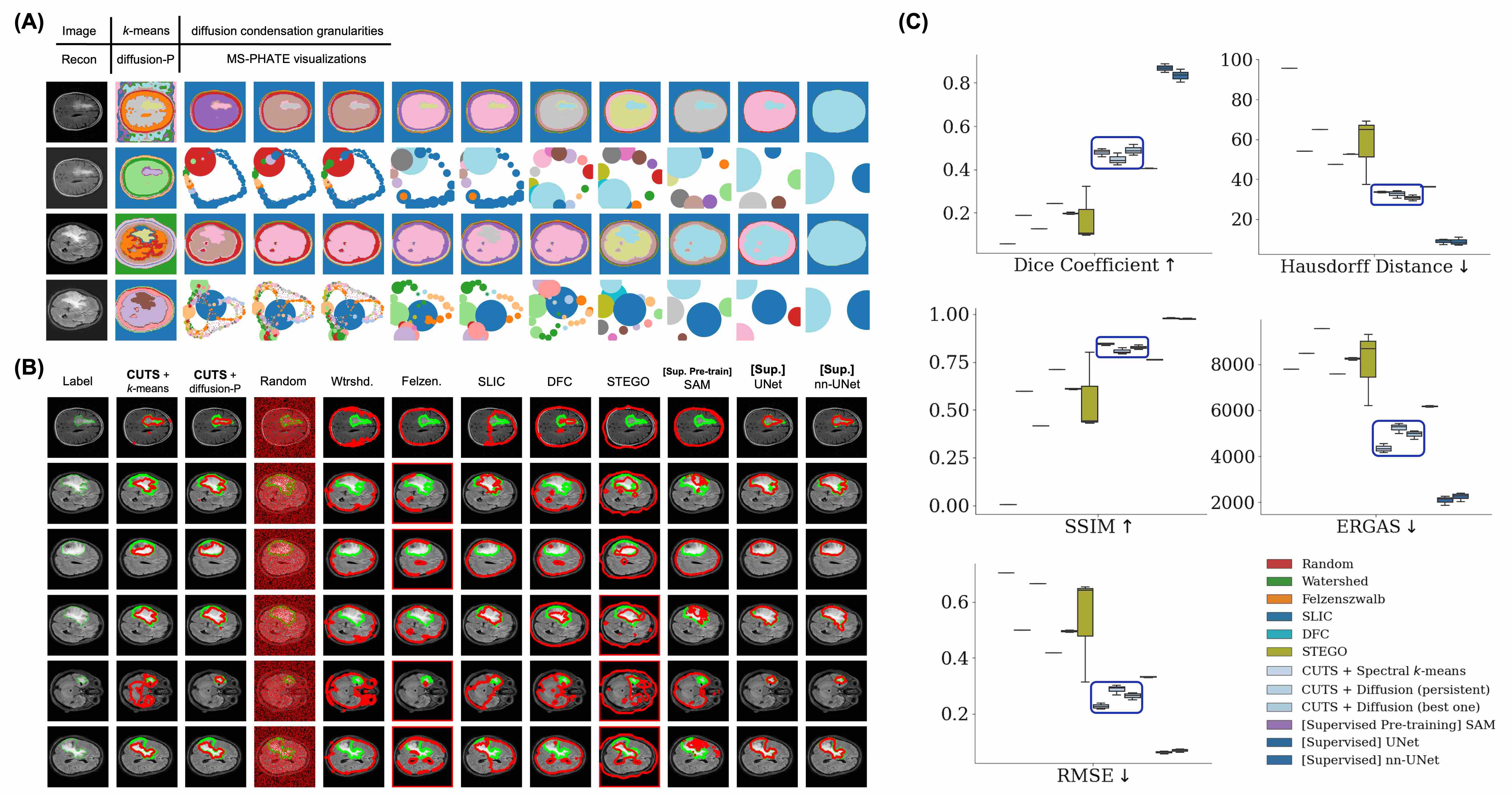
Figure 5: Segmenting tumors in brain MRI images. (A) Multigranular segmentation (odd rows) captures distinctive patterns at various scales. Multiscale PHATE (even rows) is used to visualize the diffusion condensation process. The results of CUTS + spectral $k$-means clustering (labeled as: $k$-means) and CUTS + diffusion condensation persistent structures (labeled as: diffusion-P) are also shown for reference. (B) Additional sample images in the format of Fig. 2. (C) Quantitative comparisons. An up arrow next to a metric indicates that a higher score is better, and an down arrow otherwise. The methods are displayed in the same order as the legends. CUTS results are highlighted by boxes. Note that SAM, UNet, and nn-UNet are not unsupervised methods.

4.3 Tumor segmentation in brain MRI images

Our final experiment investigated the performance of CUTS on a different segmentation target in brain MRI images — brain tumors, or more specifically, glioma. Accurate segmentation of tumor areas is crucial for the diagnosis and treatment of brain tumors. This process can assist radiologists in providing vital details about the size, position, and form of tumors, which is important in determining the most appropriate course of clinical care.

Challenges in this dataset include variability in tumor appearance, heterogeneity of tissue types, as well as infiltration into adjacent brain regions that makes it difficult to define tumor boundaries. Furthermore, the intrinsic properties of MRI as previously described contribute to the difficulty of this task.

4.3.1 Qualitative results

Our method is successful in segmenting tumor regions in brain MRI, as shown in Fig. 5(A). Our method operates across a range of scales, starting with the identification of brain ventricles that stand out prominently against surrounding tissues due to their high contrast. As we progress to finer scales, our method becomes capable of isolating tumor regions. However, unlike the previous experiment that focused on ventricle segmentation, our method does not distinguish between gray and white matter in this particular task. This discrepancy can be attributed to variations in the MRI modalities used in the datasets, as well as the notably pronounced contrast of tumor regions in this specific dataset. Once again, our method provides clinicians with the ability to quantify relevant features at different levels of detail. Moreover, the experiments conducted on three distinct medical imaging datasets illustrate the meaningful results our method can achieve, despite the significant differences in the underlying physics principles and the resulting image characteristics of these imaging technologies.

Table 1: Quantitative comparisons of CUTS and existing methods. Mean values are reported from 3 independent runs with different random seeds. Among the unsupervised methods, the best performances are highlighted in bold whereas runner-ups are marked in blue. Supervised methods are included for reference. An up arrow next to a metric indicates that a higher score is better and a down arrow otherwise. ^† Strictly speaking, SAM is neither fully supervised nor unsupervised learning. It follows a large-scale pre-training & zero-shot transfer paradigm (see Related work).

		Unsupervised, w/o Learning				Unsupervised, w/ Learning					Supervised† Pre-training	Supervised
		Random	Watersh. TPAMI${}^{\prime}91$ [5]	Felzens. IJCV${}^{\prime}04$ [7]	SLIC TPAMI${}^{\prime}12$ [17]	DFC TIP${}^{\prime}20$ [42]	STEGO ICLR${}^{\prime}22$ [43]	CUTS + Spectral $k$-means	CUTS + Diffusion (persist.)	CUTS + Diffusion (best one)	SAM ICCV${}^{\prime}23$, MedIA${}^{\prime}23$ [44, 45]	UNet MICCAI${}^{\prime}15$ [18]	nnUNet Nat.Mth.${}^{\prime}21$ [24]
Retina Geographic Atrophy	Dice $\uparrow$	0.132	0.187	0.222	0.567	0.300	0.649	0.673	0.685	0.735	0.924	0.965	0.937
	Hausdorff $\downarrow$	78.44	61.60	64.05	28.76	46.47	34.12	27.75	27.43	25.28	9.18	3.78	6.00
	SSIM $\uparrow$	0.000	0.177	0.164	0.779	0.400	0.842	0.871	0.842	0.874	0.944	0.976	0.968
	ERGAS $\downarrow$	11694	13554	13176	6824	11761	7502	4687	5253	4587	3205	2179	2516
	RMSE $\downarrow$	0.707	0.825	0.833	0.323	0.641	0.250	0.216	0.241	0.203	0.100	0.062	0.077
Brain Ventricles	Dice $\uparrow$	0.150	0.631	0.716	0.475	0.631	0.725	0.774	0.628	0.819	0.644	0.989	0.984
	Hausdorff $\downarrow$	61.36	30.25	20.35	37.96	34.28	12.59	8.11	16.34	12.90	30.24	1.05	2.10
	SSIM $\uparrow$	0.000	0.845	0.838	0.683	0.648	0.849	0.879	0.840	0.878	0.894	0.990	0.986
	ERGAS $\downarrow$	22232	9275	9725	13992	12294	13495	7656	8729	7465	7168	1169	1893
	RMSE $\downarrow$	0.707	0.246	0.225	0.412	0.371	0.220	0.179	0.213	0.156	0.191	0.023	0.044
Brain Tumor	Dice $\uparrow$	0.057	0.188	0.127	0.242	0.197	0.176	0.479	0.447	0.489	0.405	0.867	0.834
	Hausdorff $\downarrow$	95.57	53.96	64.90	47.51	52.52	57.16	33.52	32.54	30.64	36.14	8.84	8.64
	SSIM $\uparrow$	0.005	0.597	0.416	0.711	0.609	0.558	0.843	0.806	0.827	0.762	0.979	0.976
	ERGAS $\downarrow$	7790	8476	9555	7594	8252	8076	4341	5238	4948	6176	2087	2235
	RMSE $\downarrow$	0.704	0.500	0.666	0.418	0.495	0.536	0.227	0.287	0.263	0.332	0.061	0.068

In the binary segmentation setting, CUTS demonstrates superior segmentation compared to other unsupervised methods, as shown in Fig. 5(B). As a general observation, competing methods struggle to identify tumor regions, although they manage to segment ventricles in a similar imaging modality. This disparity in performance was anticipated, given the pronounced complexity associated with tumor segmentation compared to ventricles, due to considerably more subtle contrast and morphological distinctions. Nevertheless, CUTS overcomes the inherent challenges and successfully segments tumor regions.

4.3.2 Quantitative results

We observe a consistent trend in which CUTS surpasses alternative unsupervised methods in all similarity and distance-based metrics we evaluated Fig. 5(C) and Table 1, consistent with our previous results. In arguably the most arduous dataset, CUTS demonstrates markedly increased superiority over competing approaches compared to the less demanding task of ventricle segmentation. More impressively, CUTS managed to achieve better results than SAM without relying on billions of external data.

5 Discussion

Current state-of-the-art methods for medical image segmentation are primarily supervised and therefore require domain experts to annotate a large number of medical images. Moreover, it is often infeasible to collect enough images of rare diseases to train supervised learning models. For example, in this work we studied a retinal degeneration condition. The number of images available to any institution of this condition is usually within a hundred, several orders of magnitude fewer than popular natural image databases for deep learning with millions of images. Furthermore, another limitation of supervised learning approaches is the domain generalization problem. When a method is optimized for a specific type of image used for training, its performance may suffer if used on other types of image, even if they are only slightly dissimilar.

In contrast, unsupervised methods, like CUTS, while more challenging architect, do not require human expert grading and thereby circumvent this time-consuming, expensive, and labor-intensive initial step. Unsupervised methods can also be applied to much smaller datasets, ideal for rare diseases. Unfortunately, prior attempts to use unsupervised learning to segment medical images have not achieved the desired results. These unsupervised methods often yield subpar performance, despite having advantages including independence from labels and the ability to generalize to new datasets while preserving robustness.

CUTS bridges the difficulty of creating unsupervised images by using the key insight that, while an image as a whole may be hard to segment, pixels forming boundaries of image features may be detectable by their local context. Thus, CUTS features carefully architected losses for local pixel-centered patch reconstruction and pixel-centered patch-based contrastive losses based on within-image augmentation of patches. With these unique penalties, CUTS learns an intermediate representation of a pixel-centered patch embedding for each image. The key advantage of this pixel-centered patch representation is that it is amenable to not one segmentation, but several multigranular segmentations of the same image via a topological coarse-graining scheme. The final output of CUTS is thus several segmentations of the image with features of different resolutions of interest for different clinical queries.

In our brain tumor image dataset, for example, CUTS enables: (1) brain extraction on the coarsest scale, (2) isolation of white matter, gray matter, and cerebrospinal fluid on the intermediate scale, and (3) small tumor segmentation on the finest scale. These different features can be important for different diagnostic purposes such as tumor placement identification for surgical purposes or small tumor size extraction for the analysis of metastases.

In this work, we demonstrate the application of CUTS to three medical image datasets from different medical domains. On the retinal fundus images, the watershed, Felzenszwalb, and DFC focus primarily on the contours of the retina without distinguishing the geographic atrophy regions, where the contrast is more subtle. SLIC and STEGO generally perform better, yet they tend to overestimate the region of interest. CUTS avoids all these caveats and consistently segments geographical atrophy. On brain MRI for ventricle segmentation, the watershed method often ignores the frontal or lateral half of the ventricles. Felzenszwalb, SLIC, and DFC have difficulty determining the segmentation boundary. STEGO tends to include tissues around the ventricles. CUTS is slightly more conservative on the boundary regions but nevertheless outperforms other unsupervised methods. On the brain MRI images for tumor segmentation, the watershed and Felzenszwalb methods merely isolate the entire brain from the background with no attention to detailed structures. SLIC, DFC, and STEGO either ignored the tumor region or merged it with the background. CUTS, on the other hand, is sensitive to tenuous contrast transitions in tumor regions and generates significantly better segmentations.

In conclusion, CUTS allows us to identify and highlight important medical image structures using an unsupervised learning approach. This has enormous implications for the expanding field of medical image evaluation and represents a step forward in identifying important and distinct information relevant to the clinical interpretation of images. Such interpretation of medical images is crucial to disease detection in asymptomatic individuals; examples include mammography for screening for breast cancer, teleophthalmology and automated image analysis for screening diabetes for eye disease, or vulnerable populations for macular degeneration and glaucoma, and screening of high-risk populations such as smokers for early lung cancer.

Data and code availability

The code used to produce our results is available in the following public repository under the MIT License: https://github.com/ChenLiu-1996/UnsupervisedMedicalSeg. The data analyzed during the current study are either available in the same repository or available upon reasonable request to the corresponding author.

Table of Contents [sections] [sections]l1

Appendix A Architecture of the convolutional encoder

Our encoder maps each pixel-centered patch $\mathcal{P}\in\mathbb{R}^{p\times p\times c}$ from a low-dimensional image space to a high-dimensional embedding space $\mathbb{R}^{d}$. Usually, $c$ is either 3 or 1. Examples for the former are natural images and colored medical images with R/G/B channels, while examples for the latter are intensity-only medical images such as CT or MRI images.

As it is crucial for these embedding vectors to include information regarding a local patch, using a ConvNet which intrinsically aggregates neighborhood information via the convolution operation is a natural design choice. Since a ConvNet, by definition, convolves trainable filters with local patches in a raster-scan manner, no additional work patching is needed. To ensure a one-to-one mapping during the encoding, we remove pooling layers which would otherwise reduce the in-plane resolution. As a result, each image with width $W$ and height $H$ is mapped from $\mathbb{R}^{H\times W\times c}$ to $\mathbb{R}^{H\times W\times d}$ by the convolutional encoder.

It is important to note that we do not perform explicit patching, i.e., cropping out $p\times p$ image patches, but rather we take advantage of the intrinsic property of convolution. A single convolutional layer with filters of size $k\times k$ incorporates information in the $k\times k$ neighborhood around each pixel, and this effect gets further enhanced as more layers are stacked together. The final embedding $z_{ij}$ at location $(i,j)$ gathers information from an area rather than a pixel in the input image, its size defined as the receptive field. To that end, we can claim that $z_{ij}$ is the embedding vector for the pixel-centered patch around pixel $(i,j)$ with size $p\times p$ equal to the receptive field.

In our implementation, we use four convolutional layers with $5\times 5$ filters to incorporate the broad contextual information around each pixel. As the network goes deeper, we progressively increase the number of filters to enrich the feature dimension. The final convolutional layer is equipped with $d$ filters, which allows us to project each input pixel to the same $d$-dimensional embedding space. In all our experiments, $d$ is set to 128.

The architecture of the convolutional encoder is specified in Table S1. The architecture does not contain pooling layers, since we want to ensure a one-to-one mapping from each pixel-centered patch to its corresponding pixel.

Table S1: Detailed specification of convolutional encoder model architecture.

input size	output size	module
$H\times W\times c$	$H\times W\times 16$	$\begin{bmatrix}\textrm{Conv2d}\_5\times 5\\ \textrm{BatchNorm2d}\\ \textrm{LeakyReLU}\end{bmatrix}$
$H\times W\times 16$	$H\times W\times 32$	$\begin{bmatrix}\textrm{Conv2d}\_5\times 5\\ \textrm{BatchNorm2d}\\ \textrm{LeakyReLU}\end{bmatrix}$
$H\times W\times 32$	$H\times W\times 64$	$\begin{bmatrix}\textrm{Conv2d}\_5\times 5\\ \textrm{BatchNorm2d}\\ \textrm{LeakyReLU}\end{bmatrix}$
$H\times W\times 64$	$H\times W\times 128$	$\begin{bmatrix}\textrm{Conv2d}\_5\times 5\\ \textrm{BatchNorm2d}\\ \textrm{LeakyReLU}\end{bmatrix}$

Appendix B Choice of weighting coefficient and ablation study

In order to select the appropriate weighting coefficient $\lambda$ in our loss function $loss=\lambda\cdot l_{contrastive}+(1-\lambda)\cdot l_{recon}$, we performed a series of experiments on the retina dataset. While keeping the other conditions fixed, we varied $\lambda$ at the following values: 0.001, 0.01, 0.03, 0.1, 0.5, and 0.9. Moreover, we also motivated our use of both contrastive and reconstruction losses together by performing an ablation study: we set $\lambda$ to 0 and 1 respectively for the “no contrastive loss” and “no reconstruction loss” conditions. The results of the comparison are reported in Fig. S1.

We find that the best-performing model ($\lambda=0.01$) uses both losses. This is understandable, as each provides a different necessary component to producing a meaningful embedding, and eventually a meaningful segmentation of the original image. With this information, we set $\lambda=0.01$ for all experiments in this paper.

Figure S1: Study on the effect of weighting coefficient $\lambda$ between the two objectives. All experiments are performed on the Retina GA Region dataset, evaluated by CUTS + Spectral $k$-means clustering, which serves as a proxy for all the other CUTS segmentation methods. Solid curves show the mean, while shaded regions show the standard error of the mean (SEM) over the entire dataset on a single experiment. The best results are indicated by the dashed vertical lines. Collectively, these results show that 0.01 is a good value for the weighting coefficient $\lambda$.

Appendix C Data preparation

C.1 Retinal fundus images

We extracted and manually graded digitized color fundus photographs (CFPs) from GA-positive eyes at least 1 visit in the age-related eye disease study (AREDS) group [54]. We described the grading process in a previous paper [55]. Briefly, to ensure the accuracy of GA segmentations, we excluded images with poor quality (i.e., the border of atrophic lesions could not be reliably identified by our graders), GA lesions extending beyond the imaging field, or GA lesions contiguous with peripapillary atrophy. ImageJ software [56] was employed by graders to manually segment GA lesions, outline the optic disc, and mark the foveal center. The gradings of each CFP were first performed by an independent trained non-expert grader, and were then reviewed and adjusted by an independent expert grader. A retinal specialist reviewed the segmentations and selected 56 retinal images with accurate segmentations from the dataset.

C.2 Brain MRI images (ventricles)

We used magnetic resonance images (MRIs) of patients who were enrolled in the Alzheimer’s Disease Neuroimaging Initiative study [57]. The inclusion criteria for this study have been previously described [58]. We randomly selected 100 T1-weighted brain MRIs from this study. A radiologist manually segmented the brain ventricles on these images.

C.3 Brain MRI images (tumor)

We used MRIs of patients with glioma that were scanned by several healthcare facilities within the Yale New Haven Health system. We randomly selected 200 fluid-attenuated inversion recovery (FLAIR) brain MRIs from this data source. Tumor regions are segmented by trained medical students within the Picture Authentication and Communication System (PACS) of Yale New Haven Hospital and finalized by a board certified attending neuroradiologist.

Appendix D Enlarged Segmentation Comparisons

Figure S2: Enlarged version of segmentation comparisons from Fig. 3. Segmentation masks (bottom) are shown in addition to contours (top).

Figure S3: Enlarged version of segmentation comparisons from Fig. 4. Segmentation masks (bottom) are shown in addition to contours (top).

Figure S4: Enlarged version of segmentation comparisons from Fig. 5. Segmentation masks (bottom) are shown in addition to contours (top).

References

- [1] Fu, Y. et al. A review of deep learning based methods for medical image multi-organ segmentation. Physica Medica 85, 107–122 (2021).
- [2] Acharjya, P. P., Das, R. & Ghoshal, D. Study and comparison of different edge detectors for image segmentation. Global Journal of Computer Science and Technology (2012).
- [3] Chen, X. & Pan, L. A survey of graph cuts/graph search based medical image segmentation. IEEE reviews in biomedical engineering 11, 112–124 (2018).
- [4] El Naqa, I. et al. Concurrent multimodality image segmentation by active contours for radiotherapy treatment planning a. Medical physics 34, 4738–4749 (2007).
- [5] Vincent, L. & Soille, P. Watersheds in digital spaces: an efficient algorithm based on immersion simulations. IEEE Transactions on Pattern Analysis & Machine Intelligence 13, 583–598 (1991).
- [6] Oh, H.-H., Lim, K.-T. & Chien, S.-I. An improved binarization algorithm based on a water flow model for document image with inhomogeneous backgrounds. Pattern Recognition 38, 2612–2625 (2005).
- [7] Felzenszwalb, P. F. & Huttenlocher, D. P. Efficient graph-based image segmentation. International journal of computer vision 59, 167–181 (2004).
- [8] Isgum, I. et al. Multi-atlas-based segmentation with local decision fusion—application to cardiac and aortic segmentation in ct scans. IEEE transactions on medical imaging 28, 1000–1010 (2009).
- [9] Aljabar, P., Heckemann, R. A., Hammers, A., Hajnal, J. V. & Rueckert, D. Multi-atlas based segmentation of brain images: atlas selection and its effect on accuracy. Neuroimage 46, 726–738 (2009).
- [10] Iglesias, J. E. & Sabuncu, M. R. Multi-atlas segmentation of biomedical images: a survey. Medical image analysis 24, 205–219 (2015).
- [11] LeCun, Y., Bengio, Y. & Hinton, G. Deep learning. nature 521, 436–444 (2015).
- [12] Esteva, A. et al. A guide to deep learning in healthcare. Nature medicine 25, 24–29 (2019).
- [13] Haque, I. R. I. & Neubert, J. Deep learning approaches to biomedical image segmentation. Informatics in Medicine Unlocked 18, 100297 (2020).
- [14] Minaee, S. et al. Image segmentation using deep learning: A survey. IEEE transactions on pattern analysis and machine intelligence (2021).
- [15] Abràmoff, M. D., Lavin, P. T., Birch, M., Shah, N. & Folk, J. C. Pivotal trial of an autonomous ai-based diagnostic system for detection of diabetic retinopathy in primary care offices. NPJ digital medicine 1, 1–8 (2018).
- [16] Tsai, A. et al. A shape-based approach to the segmentation of medical imagery using level sets. IEEE transactions on medical imaging 22, 137–154 (2003).
- [17] Achanta, R. et al. Slic superpixels compared to state-of-the-art superpixel methods. IEEE transactions on pattern analysis and machine intelligence 34, 2274–2282 (2012).
- [18] Ronneberger, O., Fischer, P. & Brox, T. U-net: Convolutional networks for biomedical image segmentation. In International Conference on Medical image computing and computer-assisted intervention, 234–241 (Springer, 2015).
- [19] Zhou, Z., Rahman Siddiquee, M. M., Tajbakhsh, N. & Liang, J. Unet++: A nested u-net architecture for medical image segmentation. In Deep learning in medical image analysis and multimodal learning for clinical decision support, 3–11 (Springer, 2018).
- [20] Oktay, O. et al. Attention u-net: Learning where to look for the pancreas. arXiv preprint arXiv:1804.03999 (2018).
- [21] Çiçek, Ö., Abdulkadir, A., Lienkamp, S. S., Brox, T. & Ronneberger, O. 3d u-net: learning dense volumetric segmentation from sparse annotation. In International conference on medical image computing and computer-assisted intervention, 424–432 (Springer, 2016).
- [22] Kohl, S. et al. A probabilistic u-net for segmentation of ambiguous images. Advances in neural information processing systems 31 (2018).
- [23] Yu, X. et al. Unest: local spatial representation learning with hierarchical transformer for efficient medical segmentation. Medical Image Analysis 90, 102939 (2023).
- [24] Isensee, F., Jaeger, P. F., Kohl, S. A., Petersen, J. & Maier-Hein, K. H. nnu-net: a self-configuring method for deep learning-based biomedical image segmentation. Nature methods 18, 203–211 (2021).
- [25] Mondal, A. K., Dolz, J. & Desrosiers, C. Few-shot 3d multi-modal medical image segmentation using generative adversarial learning. arXiv preprint arXiv:1810.12241 (2018).
- [26] Ouyang, C., Kamnitsas, K., Biffi, C., Duan, J. & Rueckert, D. Data efficient unsupervised domain adaptation for cross-modality image segmentation. In Medical Image Computing and Computer Assisted Intervention–MICCAI 2019: 22nd International Conference, Shenzhen, China, October 13–17, 2019, Proceedings, Part II 22, 669–677 (Springer, 2019).
- [27] Yu, H. et al. Foal: Fast online adaptive learning for cardiac motion estimation. In Proceedings of the IEEE/CVF conference on computer vision and pattern recognition, 4313–4323 (2020).
- [28] Chen, C. et al. Realistic adversarial data augmentation for mr image segmentation. In Medical Image Computing and Computer Assisted Intervention–MICCAI 2020: 23rd International Conference, Lima, Peru, October 4–8, 2020, Proceedings, Part I 23, 667–677 (Springer, 2020).
- [29] Yang, Q. et al. Label efficient segmentation of single slice thigh ct with two-stage pseudo labels. Journal of Medical Imaging 9, 052405–052405 (2022).
- [30] Ouyang, C. et al. Self-supervision with superpixels: Training few-shot medical image segmentation without annotation. In Computer Vision–ECCV 2020: 16th European Conference, Glasgow, UK, August 23–28, 2020, Proceedings, Part XXIX 16, 762–780 (Springer, 2020).
- [31] Nan, Y. et al. Unsupervised tissue segmentation via deep constrained gaussian network. IEEE Transactions on Medical Imaging 41, 3799–3811 (2022).
- [32] Zhao, A., Balakrishnan, G., Durand, F., Guttag, J. V. & Dalca, A. V. Data augmentation using learned transformations for one-shot medical image segmentation. In Proceedings of the IEEE/CVF conference on computer vision and pattern recognition, 8543–8553 (2019).
- [33] Wang, S. et al. Lt-net: Label transfer by learning reversible voxel-wise correspondence for one-shot medical image segmentation. In Proceedings of the IEEE/CVF Conference on Computer Vision and Pattern Recognition, 9162–9171 (2020).
- [34] Chen, T., Kornblith, S., Norouzi, M. & Hinton, G. A simple framework for contrastive learning of visual representations (2020). 2002.05709.
- [35] Caron, M. et al. Unsupervised learning of visual features by contrasting cluster assignments. Advances in Neural Information Processing Systems 33, 9912–9924 (2020).
- [36] He, K., Fan, H., Wu, Y., Xie, S. & Girshick, R. Momentum contrast for unsupervised visual representation learning. In Proceedings of the IEEE/CVF conference on computer vision and pattern recognition, 9729–9738 (2020).
- [37] Grill, J.-B. et al. Bootstrap your own latent-a new approach to self-supervised learning. Advances in neural information processing systems 33, 21271–21284 (2020).
- [38] Zbontar, J., Jing, L., Misra, I., LeCun, Y. & Deny, S. Barlow twins: Self-supervised learning via redundancy reduction. In International Conference on Machine Learning, 12310–12320 (PMLR, 2021).
- [39] Chen, X. & He, K. Exploring simple siamese representation learning. In Proceedings of the IEEE/CVF Conference on Computer Vision and Pattern Recognition, 15750–15758 (2021).
- [40] Chaitanya, K., Erdil, E., Karani, N. & Konukoglu, E. Contrastive learning of global and local features for medical image segmentation with limited annotations (2020). 2006.10511.
- [41] Yan, K. et al. Self-supervised learning of pixel-wise anatomical embeddings in radiological images (2020). 2012.02383.
- [42] Kim, W., Kanezaki, A. & Tanaka, M. Unsupervised learning of image segmentation based on differentiable feature clustering. IEEE Transactions on Image Processing 29, 8055–8068 (2020).
- [43] Hamilton, M., Zhang, Z., Hariharan, B., Snavely, N. & Freeman, W. T. Unsupervised semantic segmentation by distilling feature correspondences. In International Conference on Learning Representations (2022).
- [44] Kirillov, A. et al. Segment anything. arXiv:2304.02643 (2023).
- [45] Mazurowski, M. A. et al. Segment anything model for medical image analysis: an experimental study. Medical Image Analysis 102918 (2023).
- [46] Kuchroo, M. et al. Multiscale phate identifies multimodal signatures of covid-19. Nature biotechnology 40, 681–691 (2022).
- [47] Hore, A. & Ziou, D. Image quality metrics: Psnr vs. ssim. In 2010 20th international conference on pattern recognition, 2366–2369 (IEEE, 2010).
- [48] Brugnone, N. et al. Coarse graining of data via inhomogeneous diffusion condensation. In 2019 IEEE International Conference on Big Data (Big Data), 2624–2633 (IEEE, 2019).
- [49] Kuchroo, M. et al. Single-cell analysis reveals inflammatory interactions driving macular degeneration. Nature Communications 14, 2589 (2023).
- [50] Coifman, R. R. & Lafon, S. Diffusion maps. Applied and computational harmonic analysis 21, 5–30 (2006).
- [51] Zha, H., He, X., Ding, C., Gu, M. & Simon, H. Spectral relaxation for k-means clustering. Advances in neural information processing systems 14 (2001).
- [52] Carmichael, O. T. et al. Ventricular volume and dementia progression in the cardiovascular health study. Neurobiology of aging 28, 389–397 (2007).
- [53] Ott, B. R. et al. Brain ventricular volume and cerebrospinal fluid biomarkers of alzheimer’s disease. Journal of Alzheimer’s disease 20, 647–657 (2010).
- [54] Davis, M. D. et al. The age-related eye disease study severity scale for age-related macular degeneration: Areds report no. 17. Archives of ophthalmology (Chicago, Ill.: 1960) 123, 1484–1498 (2005).
- [55] Shen, L. L. et al. Relationship of topographic distribution of geographic atrophy to visual acuity in nonexudative age-related macular degeneration. Ophthalmology Retina 5, 761–774 (2021).
- [56] Rueden, C. T. & Eliceiri, K. W. Imagej for the next generation of scientific image data. Microscopy and Microanalysis 25, 142–143 (2019).
- [57] Crawford, K. L., Neu, S. C. & Toga, A. W. The image and data archive at the laboratory of neuro imaging. Neuroimage 124, 1080–1083 (2016).
- [58] Mueller, S. G. et al. The alzheimer’s disease neuroimaging initiative. Neuroimaging Clinics 15, 869–877 (2005).
Table of Contents \startcontents[sections] \printcontents[sections]l1