Microstructural Pattern Formation during Far-from-Equilibrium Alloy Solidification

Abstract

We introduce a new phase-field formulation of rapid alloy solidification that quantitatively incorporates nonequilibrium effects at the solid-liquid interface over a very wide range of interface velocities. Simulations identify a new dynamical instability of dendrite tip growth driven by solute trapping at velocities approaching the absolute stability limit. They also reproduce the formation of the widely observed banded microstructures, revealing how this instability triggers transitions between dendritic and microsegregation-free solidification. Predicted band spacings agree quantitatively with observations in rapidly solidified Al-Cu thin films.

The past two decades have witnessed major progress in modeling complex interface patterns that form during alloy solidification. A major contributor to this progress has been the advent of the phase-field (PF) method [1, 2, 3, 4, 5], which circumvents front tracking by making the solid-liquid interface spatially diffuse over some finite width $\sim W$, and the development of quantitative PF formulations [6, 7, 8, 9, 10, 11] that have enabled simulations on experimentally relevant length and timescales with a computationally tractable choice of $W$ on the pattern scale [12, 13, 14, 15, 16, 17, 18].

Morphological instability driving microstructural pattern formation occurs over an extremely wide range of solidification velocities $V$ spanning six orders of magnitude from $\mu$m/s to m/s, with different ranges of $V$ relevant for different solidification processes from conventional casting to metal additive manufacturing [19, 20]. To date, however, PF formulations to quantitatively simulate alloy solidification patterns have been primarily developed and validated for slow $V$ [7, 8], conditions under which the solid-liquid interface can be assumed to remain in local thermodynamic equilibrium. While there have been attempts to extend quantitative modeling to rapid solidification, existing PF formulations have been limited to a small departure from equilibrium [21], or have only reproduced solute trapping in one-dimensional (1D) simulations for larger $V$ [22, 23, 24, 25]. Simulating quantitatively far-from-equilibrium conditions, which is relevant for a host of rapid solidification processes, has remained a major challenge.

In this Letter, we develop a PF formulation to quantitatively model dilute alloy solidification under far-from-equilibrium conditions with a computationally tractable choice of $W$ on the pattern scale. The model incorporates well-known nonequilibrium effects, including solute trapping characterized by $V$-dependent forms of the partition coefficient $k(V)$ and liquidus slope $m(V)$ and interface kinetics. Simulations reproduce the formation of banded microstructures [26, 27, 28, 29, 30, 31, 32, 33, 34, 35] with a band spacing that is in remarkably good quantitative agreement with observations in thin-films of rapidly solidified Al-Cu alloys [35]. They further reveal that steady-state dendritic array growth is terminated by a novel dendrite tip instability driven by solute trapping that initiates banding.

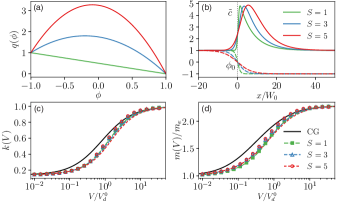
Figure 1: (a) Plots of $q(\phi)$ for $S=1,3,5$ ($A=1,6,12$), with (b) corresponding PF $\phi=\phi_{0}$ and normalized concentration $\tilde{c}=c/c_{\infty}$ profiles obtained from the numerical solution of Eq. (5). (c) $k(V)$ and (d) $m(V)$ functions obtained from the full (symbols) and approximate (dashed lines) solutions (see text). The black solid lines in (c) and (d) represent the CG model with coefficients derived in the large-velocity asymptotic limit [36].

PF models have been shown to reproduce solute trapping properties [22, 37, 23, 24, 25, 38], quantitatively for a physical choice of interface thickness $W_{0}\sim 1$ nm. Computations on a microstructural length scale, however, generally require choosing the interface thickness in the PF model, $W\gg W_{0}$, thereby producing spurious excess trapping. For the low-velocity solidification regime, this problem has been circumvented by the introduction of an antitrapping current that eliminates excess solute trapping to restore local equilibrium at the interface [7, 8]. The form of this current has been modified to also model a moderate departure from equilibrium [21, 39]. However, a quantitative approach remains lacking to describe far-from-equilibrium phenomena such as banding. Here, we follow a different approach where excess trapping resulting from the computational constraint $S\equiv W/W_{0}\gg 1$ is compensated by enhancing the solute diffusivity $D(\phi)\equiv D_{l}q(\phi)$ in the spatially diffuse interface region. We show that, remarkably, simple forms of $q(\phi)$ can be used to reproduce quantitatively the desired velocity-dependent forms of $k(V)$ and $m(V)$ over a several orders of magnitude variation of $V$ from near ($k(V)\rightarrow k_{e}$ where $k_{e}$ is the equilibrium value of the partition coefficient) to far from ($k(V)\rightarrow 1$) equilibrium conditions. This approach has the advantage that it can be implemented in a variational formulation of the PF evolution equations that can be readily extended to general binary or multicomponent alloys.

We present the model for the simplest case of a dilute binary alloy where the evolution equations

$$\tau(\mathbf{n})\frac{\partial\phi}{\partial t}= \vec{\nabla}\cdot\left[W(\mathbf{n})^{2}\vec{\nabla}\phi\right]+\phi-\phi^{3}$$

$$+\sum_{i=x,y}\left[\partial_{i}\left(|\vec{\nabla}\phi|^{2}W(\mathbf{n})\frac{\partial W(\mathbf{n})}{\partial\left(\partial_{i}\phi\right)}\right)\right]$$

$$-\lambda g^{\prime}(\phi)\left[c+\frac{\left(T-T_{M}\right)}{m_{e}}e^{b(1+g(\phi))}\right],$$ (1)

$$\frac{\partial c}{\partial t}= \vec{\nabla}\cdot\left\{D_{l}q(\phi)c\vec{\nabla}[\ln c-bg(\phi)]\right\},$$ (2)

are derived variationally from the free-energy functional introduced in [37] and defined here by Eqs. (S3)-(S6) in the Supplemental Material [36]. Together with the relations $b\equiv\ln k_{e}/2<0$, $\tau_{0}=(SW_{0})^{2}/(\Gamma\mu_{k}^{0})$, and $\lambda=a_{1}^{0}bm_{e}SW_{0}/[\Gamma(k_{e}-1)]>0$ between PF and materials parameters [37], where $\Gamma=\gamma_{0}T_{M}/L$ is the Gibbs-Thomson coefficient, $T_{M}$ is the melting point, $L$ is the latent heat of melting, $m_{e}>0$ is the equilibrium value of the liquidus slope, and $a_{1}^{0}=SW_{0}\int_{-\infty}^{\infty}dx(d\phi_{0}/dx)^{2}=2\sqrt{2}/3$, the choices of interface width $W(\mathbf{n})=SW_{0}a_{s}(\mathbf{n})$ and time constant $\tau(\mathbf{n})=\tau_{0}a_{s}(\mathbf{n})^{2}/a_{k}(\mathbf{n})$ model general anisotropic forms of the excess free-energy of the solid-liquid interface $\gamma(\mathbf{n})=\gamma_{0}a_{s}(\mathbf{n})$ and interface kinetic coefficient $\mu_{k}(\mathbf{n})=\mu_{k}^{0}a_{k}(\mathbf{n})$, where $\mathbf{n}$ is the direction normal to the interface. In addition, we use the common choice $g(\phi)=15(\phi-2\phi^{3}/3+\phi^{5}/5)/8$ that satisfies $g^{\prime}(\pm 1)=g^{\prime\prime}(\pm 1)=0$ and guarantees that the local minima of the free-energy density remain at $\phi=\pm 1$ for arbitrarily large thermodynamic driving force.

For the one-sided model of alloy solidification, $q(\phi)=(1-\phi)/2$ is the simplest form that describes the physically expected monotonous decrease of diffusivity from liquid to solid across the interface. This form, however, produces spurious excess trapping at lower $V$ when $S\gg 1$, since the diffusive speed in the PF model $V_{d}\sim D_{l}/W\sim V_{d}^{0}/S$, where $V_{d}^{0}\equiv D_{l}/W_{0}$. Hence, to eliminate excess trapping, we use the quadratic form $q(\phi)=A(1-\phi)/2-(A-1)(1-\phi)^{2}/4$ that enhances $D(\phi)$ in the interface region for $A>1$ (Fig. 1(a)).

We show next how this form of $q(\phi)$ can be used to reproduce $S$-independent solute trapping properties. For this, we look for steady-state PF and concentration profiles corresponding to a planar isothermal interface moving at constant velocity $V$. Those profiles are determined by rewriting Eqs. (1)-(2) in a frame moving with the interface at velocity $V$ in the $x$ direction

$$-\tau_{0}V\frac{d\phi}{dx} =(SW_{0})^{2}\frac{d^{2}\phi}{dx^{2}}+\phi-\phi^{3}$$

$$- \lambda g^{\prime}(\phi)\left[c+\frac{(T-T_{M})}{m_{e}}e^{b(1+g(\phi))}\right],$$ (3)

$$-V\frac{dc}{dx} =\frac{d}{dx}\left(D_{l}q(\phi)c\frac{d}{dx}[\ln c-bg(\phi)]\right),$$ (4)

where we have considered for simplicity the isotropic case $a_{s}(\mathbf{n})=a_{k}(\mathbf{n})=1$. Eq. (4) can be simplified further by integrating both sides once with respect to $x$ and using the boundary condition $c(\pm\infty)=c_{\infty}$ imposed by mass conservation, yielding

$$\frac{dc}{dx}=(c_{\infty}-c)\frac{V}{D_{l}q(\phi)}+b\,c\,\frac{dg(\phi)}{dx}.$$ (5)

In addition, a self-consistent expression for the velocity-dependent temperature is obtained by multiplying both sides of Eq. (3) by $d\phi/dx$ and integrating over $x$ from $-\infty$ to $+\infty$, yielding

$$T(V)=T_{M}-\frac{b\,m_{e}}{1-k_{e}}\int_{-\infty}^{\infty}dx\,g^{\prime}(\phi)\,c\,\frac{d\phi}{dx}+\frac{a_{1}b\,m_{e}}{\lambda(1-k_{e})}\frac{\tau_{0}V}{SW_{0}},$$ (6)

where we have defined $a_{1}=SW_{0}\int_{-\infty}^{\infty}dx(d\phi/dx)^{2}$. The solution of Eqs. (3) and (5) with $T$ given by Eq. (6) and the boundary condition $c(\pm\infty)=c_{\infty}$ uniquely determine the steady-state profile $\phi(x)$ and $c(x)$. The “full solution” to this system of equations is straightforward to obtain numerically by a procedure that will be described in more detail elsewhere. An “approximate solution” very close to the full solution can also be obtained by assuming that the PF profile for a moving interface remains close to its stationary profile $\phi_{0}(x)=-\tanh{[{x}/{(\sqrt{2}W})]}$. In this approximation, the concentration profile is solely determined by Eq. (5), which is readily solved by numerical integration to obtain the concentration profiles shown in Fig. 1(b). $T(V)$ is then determined by Eq. (6) with those $c$ profiles and $\phi(x)=\phi_{0}(x)$. Finally, the corresponding functions $k(V)$ and $m(V)$ are obtained from the sharp-interface relations $k(V)=c_{s}/c_{l}$ and

$$T(V)=T_{M}-m(V)c_{l}-{V}/{\mu_{k}},$$ (7)

where $c_{s}$ and $c_{l}$ are the concentrations on the solid and liquid sides of the interface, respectively, which correspond here to $c_{\infty}$ and the peak value of $c(x)$. Matching the second and third terms on the right-hand side of Eqs. (6) and (7), yields at once

$$\frac{m(V)}{m_{e}}=\frac{b}{(1-k_{e})c_{l}}\int_{-\infty}^{\infty}dxg^{\prime}(\phi)c\frac{d\phi}{dx},$$ (8)

and $\mu_{k}=\mu_{k}^{0}a_{1}^{0}/a_{1}$, respectively. To obtain values of $A$ that yield $S$-independent trapping properties, we first compute reference $k(V)$ and $m(V)$ curves corresponding to $S=1$ and $A=1$. For a given $S>1$, we then compute $k(V)$ and $m(V)$ curves for different $A$ values and find the value of $A$ that minimizes the departure from the reference curves over some large velocity range of interest. This procedure is implemented with the approximate ($\phi=\phi_{0}$) solution and yields $A=6$ and 12 for $S=3$ and 5, respectively, for parameters of Al-Cu alloys [36]. Plots of $k(V)$ and $m(V)$ obtained from the approximate ($\phi=\phi_{0}$) and full solutions of the steady-state concentration and PF profiles are shown for the different $S$ and corresponding $A$ values in Figs. 1(c)-(d), respectively. The approximate solution only depends on $k_{e}$ and yields $\mu_{k}=\mu_{k}^{0}$ while the full solution depends on the other alloy parameters, and the deviation of $\phi$ from $\phi_{0}$ at larger $V/V_{d}^{0}$ causes a small quantitative difference between the two solutions. Remarkably, even though a single parameter $A$ is optimized for each $S$, $k(V)$ and $m(V)$ are seen to be nearly independent of $S$ over a several orders magnitude variation of $V$. Even though the concentration profiles depend on $S$ (Fig. 1(b)), they have almost identical peak values, which determine $k(V)$, and the different profiles also yield nearly identical values of $m(V)$ via Eq. (8).

The $k(V)$ and $m(V)$ functions are compared to the predictions of the continuous growth (CG) model as in [22] by extracting the diffusive speed $V_{d}$ from the asymptotic analytical solution of Eq. (5) for $V\gg V_{d}^{0}$ and $S=1$, assuming $\phi=\phi_{0}$, and concomitantly the solute drag coefficient $\alpha$ from Eq. (8). This calculation yields $V_{d}\approx 0.356V_{d}^{0}\ln(1/k_{e})/(1-k_{e})$ and $\alpha\approx 0.645$ [36]. Since the PF model resolves the spatially diffuse interface region, while the CG model is a sharp-interface description, quantitative agreement between the two models over the entire range of $V$ for different $k_{e}$ is not generally expected, even though agreement becomes almost perfect for larger $k_{e}$ [36]. More than the PF and CG models comparison, what is important here is that the PF $k(V)$ and $m(V)$ curves for a realistic width $(S=1)$ can be reproduced for a much larger width ($S\gg 1$) to make simulations on a microstructural scale feasible. Parameters of the PF model (e.g., $W_{0}$ and the functions $q(\phi)$ and $g(\phi)$) can, in addition, be further adjusted to better fit desired $k(V)$ and $m(V)$ curves.

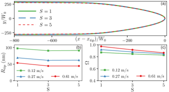
Figure 2: (a) Comparison of steady-state interface shapes for different $S$ from 2D PF simulations of dendritic array growth for Al-3wt.% Cu, $V_{p}=0.12$ m/s, and $G=5\times 10^{6}$ K/m. (b) Tip radius $R_{\mathrm{tip}}$ and (c) dimensionless tip supersaturation $\Omega$ versus $S$ for different $V_{p}$.

To validate our approach for such simulations, we model the two-dimensional (2D) directional solidification of dilute Al-Cu alloys. We consider first the standard frozen temperature approximation (FTA) that neglects latent-heat rejection, which corresponds to replacing ${\left(T-T_{M}\right)}/{m_{e}}$ in Eq. (1) by $G(x-x_{0}-V_{p}t)/m_{e}-c_{\infty}$, where $V_{p}$ is the pulling speed of the sample, $G$ is the externally imposed temperature gradient, and $x_{0}$ coincides with the equilibrium liquidus temperature $T_{L}-m_{e}c_{\infty}$. In addition, we consider anisotropic forms of the excess interface free-energy $a_{s}(\theta)=1+\epsilon_{s}\cos(4\theta)$, and kinetic coefficient $a_{k}(\theta)=1+\epsilon_{k}\cos(4\theta)$, with fourfold symmetry, where $\theta$ is the angle between $\mathbf{n}$ and the $x$ axis.

To investigate the convergence of the method, we first focus on the velocity range below the onset of banding where stable dendritic array structures are formed. This allows us to compare, for different $S$, steady-state interface shapes corresponding to a single dendrite obtained using periodic boundary conditions in $y$, with the width of the simulation domain along $y$ equal to the primary dendrite array spacing $\Lambda$ (0.65 $\mu$m), chosen within the stable range of $\Lambda$. This comparison in Fig. 2(a) shows that different $S$ yield nearly identical shapes, and the computation time is reduced by three orders of magnitude for $S=5$ compared to $S=1$ [36]. Results in Fig. 2(b) characterize steady-state shapes by the tip radius $R_{\mathrm{tip}}$ and dimensionless tip supersaturation $\Omega=(c_{l}-c_{\infty})/(c_{l}-c_{s})$. The latter is relatively well described by the Ivantsov relation between $\Omega$ and Péclet number $R_{\mathrm{tip}}V_{p}/(2D_{l})$ [36]. Quantitative differences between different $S$ for larger $V_{p}$ are likely due to other effects, such as surface diffusion and interface stretching known to affect pattern selection [7, 8]. While those effects can be eliminated in the framework of the thin-interface limit for quasi-equilibrium growth conditions, eliminating them for the entire $V$ range of Figs. 1(c)-(d) is considerably more challenging. Fig. 2 shows that, even with such effects present, the method converges already reasonably well.

Next, we exploit the model to address basic open questions of interface dynamics in this regime using $S=5$ for efficiency. The first is how steady-state dendrite array growth illustrated in Fig. 2(a) loses stability to trigger banding as $V_{p}$ approaches the absolute stability limit $V_{a}$ defined implicitly by the relation [40, 41, 42, 43]

$$V_{a}=\frac{D_{l}m(V_{a})c_{\infty}\left[1-k(V_{a})\right]}{k(V_{a})^{2}\Gamma},$$ (9)

where $k(V)$ and $m(V)$ are computed as before from the full solution of the 1D PF Eqs. (3) and (5) with $T(V)$ given by Eq. (6), but with the substitutions $SW_{0}\rightarrow SW_{0}(1+\epsilon_{s})$ and $\tau_{0}\rightarrow\tau_{0}(1+\epsilon_{k})$ in Eq. (3) to account for anisotropy. To address this question, we performed a simulation in the same geometry Fig. 2(a) but with $V_{p}$ slowly increasing linearly in time on a timescale much longer than the characteristic time for the interface to relax to a steady-state shape, thereby allowing us to probe pattern stability over a large range of $V_{p}$. We find that above a critical velocity $V_{c}\approx 0.88$ m/s steady-state growth becomes unstable as illustrated by the time sequence in Fig. 3(a). This instability is highly localized at the dendrite tip and triggers a rapid “burgeoning-like” growth of the interface. Fig. 3(b) shows that this abrupt acceleration of the interface is accompanied by a rapid drop in $c_{l}$ associated with almost complete solute trapping, followed by a rapid deceleration of the interface and increase of $c_{l}$ as the interface transits to a planar morphology and the diffusion boundary layer rebuilds itself.

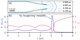
Figure 3: (a) Evolution of the solid-liquid interface illustrating the burgeoning tip instability at $V_{p}=V_{c}=0.88$ m/s for Al-3wt.% Cu and $G=5\times 10^{6}$ K/m (see movie in [36]). (b) Corresponding tip velocity $V$ and scaled interface concentration $\tilde{c}_{l}=c_{l}/c_{\infty}$ on the liquid side.

The onset velocity $V_{c}$ of instability depends on the anisotropy parameters $\epsilon_{s}$ and $\epsilon_{k}$ that are known to control dendrite tip selection [44, 45, 46, 47] and do not enter in the linear stability analysis used to predict $V_{a}$. However, for the parameters of our simulations, $V_{c}$ turns out to be close to the value $V_{a}\approx 0.86$ m/s predicted by Eq. (9). Moreover, the simulation of Fig. 3 was purposely carried out without thermal noise to study the basic instability of steady-state shapes. Additional simulations with noise-induced sidebranching reveal that the burgeoning instability can also emerge from the tips of secondary branches, especially for larger $\Lambda$ that accommodates larger amplitude sidebranches.

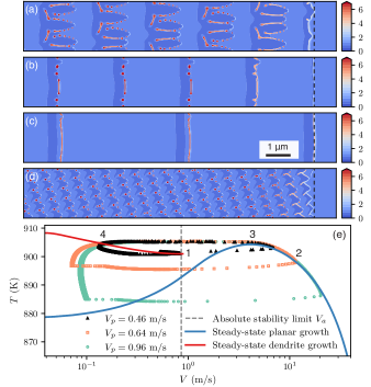
Figure 4: Microsegregation patterns ($\tilde{c}=c/c_{\infty}$ color maps) simulated for Al-3wt.% Cu with $G=5\times 10^{6}$ K/m and the FTA for $V_{p}=$ (a) 0.46, (b) 0.64, and (c) 0.96 m/s, and with latent heat for (d) $V_{p}=0.96$ m/s; black dashed lines mark solidification front positions. (e) Steady-state curves and banding cycles in the $T-V$ plane. Movies corresponding to (a) and (d) are shown in the Supplemental Material [36].

Next, we investigate banding by using the FTA and the method developed in [16] to include latent-heat rejection at the interface. Figs. 4(a)-(c) show the microstructures obtained with the FTA at three increasing values of $V_{p}$ and Fig. 4(d) shows the pattern obtained at the largest $V_{p}$ with latent heat for comparison. The oscillation cycles corresponding to the FTA simulations of Figs. 4(a)-(c) are shown in the $T-V$ plane of Fig. 4(e), where points along each cycle represent the temperature and velocity of the most advanced point along the solidification front at subsequent instants of time.

Superimposed on the $T-V$ plane are the steady-state curves corresponding to stable dendritic array growth (red curve) for $V<V_{c}$ and planar front growth (blue curve) computed using Eq. (7). The conceptual model of banding derived in the FTA framework assumes that the interface makes instantaneous transitions (1-2) and (3-4) between those steady-state curves, and follows those curves during the dendritic array (4-1) and planar front (2-3) growth portions of the complete 1-2-3-4-1 banding cycle, where 1 corresponds to $V_{a}$ and 3 corresponds to the maximum of the $T(V)$ curve for steady-state planar front growth. The simulated banding cycle of Fig. 4(a) follows reasonably well this conceptual cycle when microsegregated and microsegregation-free bands corresponding to dendritic array and planar front growth, respectively, are of comparable width, while the cycles of Figs. 4(b)-(c) make larger loops in the $T-V$ plane when planar front growth occupies a larger fraction of the whole banding cycle that is no longer constrained to follow the 4-1 segment corresponding to steady-state dendritic array growth.

The comparison of Fig. 4 (c) and (d) shows that latent-heat rejection dramatically reduces the band spacing from about 2 $\mu$m to 500 nm. Latent heat was previously found to reduce the period of oscillations of the planar interface [48, 49], but those 1D cycles could not predict banded microstructure formation. Fig. 4(d) reveals that bands grow at a small angle with respect to the thermal axis due to the fact that the lateral spreading velocity of the interface that produces microsegregation-free bands is slowed down by latent-heat rejection. The banding cycle is shrunk and no longer easily represented by the path of a uniquely defined solidification front in the $T-V$ plane as for FTA.

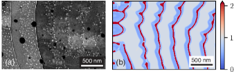
Figure 5: Comparison of banded microstructures for Al-9 wt.% Cu from (a) the late stage of a thin-film resolidification experiment (reproduced with permission from [35]), and (b) a 2D PF simulation with latent heat and $G=5\times 10^{6}$ K/m ($\tilde{c}=c/c_{\infty}$ color map).

Finally, we show in Fig. 5 a quantitative comparison of banded microstructures simulated with latent heat and produced in a resolidification experiment where a short laser pulse is used to create an elliptical melt pool in a thin film of an Al-9 wt.% (Al-4 at.%) Cu alloy [35]. Based on dynamic transmission electron microscopy (DTEM) measurements of interface velocity, $V_{p}$ was increased in the simulation linearly from 0.3 to 1.8 m/s over a time period 30 $\mathrm{\mu s}$. As shown in Fig. 5, the band spacing in simulation ($\sim 400$ nm) agrees remarkably well with the experiment. Simulations for other alloys (e.g., Al-Fe) also yield a good agreement with previous experimental observations of banded microstructures in laser remelting experiments [26, 27, 28, 29, 30, 31, 32]. They will be presented elsewhere in a longer exposition of methods and results.

We thank Wilfried Kurz for valuable discussions. This work was supported by the U.S. Department of Energy (DOE), Office of Science, Basic Energy Sciences (BES) under Award No. DE-SC0020870.

References

- Boettinger et al. [2002] W. J. Boettinger, J. A. Warren, C. Beckermann, and A. Karma, Phase-field simulation of solidification (2002).
- Steinbach [2009] I. Steinbach, Modelling and Simulation in Materials Science and Engineering 17, 073001 (2009).
- Karma and Tourret [2016] A. Karma and D. Tourret, Atomistic to continuum modeling of solidification microstructures (2016).
- Kurz et al. [2020] W. Kurz, M. Rappaz, and R. Trivedi, International Materials Reviews 66, 30 (2020).
- Tourret et al. [2022] D. Tourret, H. Liu, and J. LLorca, Progress in Materials Science 123, 100810 (2022).
- Karma and Rappel [1998] A. Karma and W. J. Rappel, Physical Review E - Statistical Physics, Plasmas, Fluids, and Related Interdisciplinary Topics , 4323 (1998).
- Karma [2001] A. Karma, Physical Review Letters , 115701 (2001).
- Echebarria et al. [2004] B. Echebarria, R. Folch, A. Karma, and M. Plapp, Physical Review E - Statistical Physics, Plasmas, Fluids, and Related Interdisciplinary Topics , 061604 (2004).
- Folch and Plapp [2005] R. Folch and M. Plapp, Physical Review E - Statistical, Nonlinear, and Soft Matter Physics 72, 011602 (2005).
- Plapp [2011] M. Plapp, Physical Review E - Statistical, Nonlinear, and Soft Matter Physics 84, 031601 (2011).
- Boussinot and Brener [2014] G. Boussinot and E. A. Brener, Physical Review E - Statistical, Nonlinear, and Soft Matter Physics 89, 060402 (2014).
- Haxhimali et al. [2006] T. Haxhimali, A. Karma, F. Gonzales, and M. Rappaz, Nature Materials 10.1038/nmat1693 (2006).
- Dantzig et al. [2013] J. A. Dantzig, P. Di Napoli, J. Friedli, and M. Rappaz, Metallurgical and Materials Transactions A: Physical Metallurgy and Materials Science 44, 5532 (2013).
- Bergeon et al. [2013] N. Bergeon, D. Tourret, L. Chen, J. M. Debierre, R. Guérin, A. Ramirez, B. Billia, A. Karma, and R. Trivedi, Physical Review Letters , 226102 (2013).
- Clarke et al. [2017] A. J. Clarke, D. Tourret, Y. Song, S. D. Imhoff, P. J. Gibbs, J. W. Gibbs, K. Fezzaa, and A. Karma, Acta Materialia 10.1016/j.actamat.2017.02.047 (2017).
- Song et al. [2018] Y. Song, D. Tourret, F. L. Mota, J. Pereda, B. Billia, N. Bergeon, R. Trivedi, and A. Karma, Acta Materialia 150, 139 (2018).
- Ghosh et al. [2018] S. Ghosh, N. Ofori-Opoku, and J. E. Guyer, Computational Materials Science 144, 256 (2018).
- Wang et al. [2020] K. Wang, G. Boussinot, C. Hüter, E. A. Brener, and R. Spatschek, Physical Review Materials 4, 033802 (2020).
- Kurz and Fisher [1989] W. Kurz and D. J. Fisher, Fundamentals of solidification (Trans Tech Publications, 1989).
- Dantzig and Rappaz [2016] J. A. Dantzig and M. Rappaz, Solidification (EPFL press, 2016).
- Pinomaa and Provatas [2019] T. Pinomaa and N. Provatas, Acta Materialia 168, 167 (2019).
- Ahmad et al. [1998] N. A. Ahmad, A. A. Wheeler, W. J. Boettinger, and G. B. McFadden, Physical Review E 58, 3436 (1998).
- Danilov and Nestler [2006] D. Danilov and B. Nestler, Acta Materialia 54, 4659 (2006).
- Steinbach et al. [2012] I. Steinbach, L. Zhang, and M. Plapp, Acta Materialia 60, 2689 (2012).
- Kavousi and Asle Zaeem [2021] S. Kavousi and M. Asle Zaeem, Acta Materialia 205, 116562 (2021).
- Boettinger et al. [1984] W. J. Boettinger, D. Shechtman, R. J. Schaefer, and F. S. Biancaniello, Metallurgical Transactions A 1984 15:1 15, 55 (1984).
- Zimmermann et al. [1991] M. Zimmermann, M. Carrard, M. Gremaud, and W. Kurz, Materials Science and Engineering: A 134, 1278 (1991).
- Gremaud et al. [1991] M. Gremaud, M. Carrard, and W. Kurz, Acta Metallurgica et Materialia 39, 1431 (1991).
- Carrard et al. [1992] M. Carrard, M. Gremaud, M. Zimmermann, and W. Kurz, Acta Metallurgica et Materialia 40, 983 (1992).
- Gill and Kurz [1993] S. C. Gill and W. Kurz, Acta Metallurgica et Materialia 41, 3563 (1993).
- Gill and Kurz [1995] S. C. Gill and W. Kurz, Acta Metallurgica et Materialia 43, 139 (1995).
- Gremaud et al. [1990] M. Gremaud, M. Carrard, and W. Kurz, Acta Metallurgica et Materialia 38, 2587 (1990).
- Kurz and Trivedi [1996] W. Kurz and R. Trivedi, Metallurgical and Materials Transactions A 1996 27:3 27, 625 (1996).
- McKeown et al. [2014] J. T. McKeown, A. K. Kulovits, C. Liu, K. Zweiacker, B. W. Reed, T. Lagrange, J. M. Wiezorek, and G. H. Campbell, Acta Materialia 65, 56 (2014).
- McKeown et al. [2016] J. T. McKeown, K. Zweiacker, C. Liu, D. R. Coughlin, A. J. Clarke, J. K. Baldwin, J. W. Gibbs, J. D. Roehling, S. D. Imhoff, P. J. Gibbs, D. Tourret, J. M. Wiezorek, and G. H. Campbell, JOM 68, 985 (2016).
- [36] See Supplemental Material at [URL will be inserted by publisher] for parameters, movies, variational formulation, continuous growth model and asymptotic analyses, and the measurement of tip supersaturation, which includes Refs. [50-57].
- Karma [2003] A. Karma, in Thermodynamics, Microstructures and Plasticity, edited by A. Finel, D. Mazière, and M. Veron (Springer, Dordrecht, 2003) pp. 65–89.
- Galenko et al. [2011] P. K. Galenko, E. V. Abramova, D. Jou, D. A. Danilov, V. G. Lebedev, and D. M. Herlach, Physical Review E - Statistical, Nonlinear, and Soft Matter Physics 84, 041143 (2011).
- Pinomaa et al. [2020] T. Pinomaa, J. M. McKeown, J. M. Wiezorek, N. Provatas, A. Laukkanen, and T. Suhonen, Journal of Crystal Growth 532, 125418 (2020).
- Mullins and Sekerka [1964] W. W. Mullins and R. F. Sekerka, Journal of Applied Physics 35, 444 (1964).
- Trivedi and Kurz [1986] R. Trivedi and W. Kurz, Acta Metallurgica 34, 1663 (1986).
- Ludwig and Kurz [1996] A. Ludwig and W. Kurz, Acta Materialia 44, 3643 (1996).
- Boettinger and A. Warren [1999] W. J. Boettinger and J. A. Warren, Journal of Crystal Growth 200, 583 (1999).
- Langer and Hong [1986] J. S. Langer and D. C. Hong, Physical Review A 34, 1462 (1986).
- Brener [1990] E. A. Brener, Journal of Crystal Growth 99, 165 (1990).
- Brener and Mel’nikov [1991] E. A. Brener and V. I. Mel’nikov, Advances in Physics 40, 53 (1991).
- Bragard et al. [2002] J. Bragard, A. Karma, Y. H. Lee, and M. Plapp, Interface Science 10, 10.1023/A:1015815928191 (2002).
- Karma and Sarkissian [1992] A. Karma and A. Sarkissian, Physical Review Letters 68, 2616 (1992).
- Karma and Sarkissian [1993] A. Karma and A. Sarkissian, Physical Review E 47, 513 (1993).
- Lee et al. [2004] J. H. Lee, S. Liu, H. Miyahara, and R. Trivedi, Metallurgical and Materials Transactions B 2004 35:5 35, 909 (2004).
- Gündüz and Hunt [1985] M. Gündüz and J. D. Hunt, Acta Metallurgica 33, 1651 (1985).
- Mendelev et al. [2010] M. I. Mendelev, M. J. Rahman, J. J. Hoyt, and M. Asta, Modelling and Simulation in Materials Science and Engineering 18, 074002 (2010).
- Ji et al. [2022] K. Ji, A. M. Tabrizi, and A. Karma, Journal of Computational Physics 457, 111069 (2022).
- Aziz [1982] M. J. Aziz, Journal of Applied Physics 53, 1158 (1982).
- Aziz and Kaplan [1988] M. J. Aziz and T. Kaplan, Acta Metallurgica 36, 2335 (1988).
- Aziz and Boettinger [1994] M. J. Aziz and W. J. Boettinger, Acta Metallurgica et Materialia 42, 527 (1994).
- Ivantsov [1947] G. P. Ivantsov, Doklady Akademii Nauk, SSSR 58 (1947).