A new reduced order model of linear parabolic PDEs

Abstract

How to build an accurate reduced order model (ROM) for multidimensional time dependent partial differential equations (PDEs) is quite open. In this paper, we propose a new ROM for linear parabolic PDEs. We prove that our new method can be orders of magnitude faster than standard solvers, and is also much less memory intensive. Under some assumptions on the problem data, we prove that the convergence rates of the new method is the same with standard solvers. Numerical experiments are presented to confirm our theoretical result.

1 Introduction

It is well known that the computational cost of solving multidimensional time dependent partial differential equations (PDEs) can be extremely high. Many model order reduction (MOR) methods have been proposed to reduce the computational cost. Proper orthogonal decomposition (POD) methods are widely used in both academic and industry [3].

There are extensive studies to prove the error bounds of the POD-ROM [26, 18, 5, 25, 20, 17, 19] under the assumption that the data in the POD-ROM are not varied from the original PDE model. However, when data is changed in the POD-ROM, the solution of the POD-ROM can be either surprisingly accurate or completely unrelated to the solution of the full order model (FOM). It is worthwhile mentioning that in [15], the authors studied the effects of small perturbations in the POD-ROM. They explained why in some applications this sensitivity is a concern while in others it is not. Therefore, hybrid methods (FOM/ROM switched back and forth) are commonly used in practice [23, 28, 10, 1]. However, the savings are not remarkable.

How to build an accurate and efficient ROM for time dependent PDEs is still an open problem. As a first step toward this open problem, we propose a new ROM for linear parabolic PDEs. Next, we briefly describe the standard finite element method (FEM) and our algorithm for solving the following heat equation:

$$\begin{split}u_{t}-\Delta u&=f(x)\quad\;\;\textup{in}\;\Omega\times(0,T],\\ u&=0\qquad\quad\textup{on}\;\partial\Omega\times(0,T],\\ u(\cdot,0)&=0\qquad\quad\textup{in}\;\Omega.\end{split}$$ (1.1)

Let $M$ and $A$ be the mass and stiffness matrices, respectively, and $b$ is the load vector. Here we assumed that the right hand side $f$ is independent of time. For general data, see Section 4. The semi-discrete of (1.1) is to find $\alpha_{h}(t)\in\mathbb{R}^{N}$ satisfying

$$\begin{split}M\alpha_{h}^{\prime}(t)+A\alpha_{h}(t)&=b,\quad t\in(0,T],\\ \alpha_{h}(0)&=0,\end{split}$$ (1.2)

where $\alpha_{h}(t)$ is the coefficient of the FEM solution under the FEM basis functions. Implicit solvers are commonly used to solve the ODE system (1.2). The computational cost can be huge (see Table 1) for solving this system. Next, we introduce our new algorithm.

• We generate a Krylov sequence for the problem data; see lines 1-4 in Algorithm 1. This is different from the standard POD method. The standard POD method uses the solution data to generate a reduced basis, which is the drawback of the method—relies too heavily on the solution data. The parameter $\ell$ we choose is a small integer, usually less than $10$. This is the main computational cost in our new algorithm. To adaptively choose $\ell$, see Algorithm 2.

• We use the idea from POD to find $r$ optimal reduced basis functions, the span of these $r$ functions generates a dimension $r$ space; see lines 5-9 in Algorithm 1.

• We project the heat equation (1.1) onto the above reduced space, and obtain the reduced mass matrix $M_{r}$, the reduced stiffness matrix $A_{r}$ and the reduced load vector $b_{r}$; see line 10 in Algorithm 1. Then the semi-discrete of the ROM is to find $\alpha_{r}(t)\in\mathbb{R}^{r}$ satisfying

  $$\begin{split}M_{r}\alpha_{r}^{\prime}(t)+A_{r}\alpha_{r}(t)&=b_{r},\qquad t\in(0,T],\\ \alpha_{r}(0)&=0.\end{split}$$ (1.3)

• For the time integration, we choose the backward Euler for the first step and then apply the two-steps backward differentiation formula (BDF2); see lines 11-14 in Algorithm 1.

• We then return to the FOM. We note that $Q\alpha_{r}^{n}$ is the coefficient of the solution at time $t_{n}$ under the standard FEM basis functions.

Algorithm 1 Our new algorithm for solving the heat equation (1.1)

Input: $\ell$, $M$, $A$, $b$, tol

1:Solve $A\texttt{u}_{1}=b$;

2:for $i=2$ to $\ell$ do

3:     Solve $A\texttt{u}_{i}=M\texttt{u}_{i-1}$;

4:end for

5:Set $U_{\ell}=[\texttt{u}_{1}\mid\texttt{u}_{2}\mid\ldots\mid\texttt{u}_{\ell}]\in\mathbb{R}^{N\times\ell}$;

6:Set $K_{\ell}=U_{\ell}^{\top}AU_{\ell}\in\mathbb{R}^{\ell\times\ell}$;

7:$[\Psi,\Lambda]=\texttt{eig}(K_{\ell})$;

8:Find minimal $r$ such that $\sum_{i=1}^{r}{\Lambda(i,i)}/\sum_{i=1}^{\ell}{\Lambda(i,i)}\geq 1-\texttt{tol}$;

9:Set $Q=U_{\ell}\Psi(:,1:r)(\Lambda(1:r;1:r))^{-1/2}$;

10:Set $M_{r}=Q^{\top}MQ$; $A_{r}=Q^{\top}AQ$; $b_{r}=Q^{\top}b$;

11:Solve $\left(\dfrac{1}{\Delta t}M_{r}+A_{r}\right)\alpha_{r}^{1}=b_{r}$;

12:for $n=2$ to $N_{T}$ do

13:     Solve $\left(\dfrac{3}{2\Delta t}M_{r}+A_{r}\right)\alpha_{r}^{n}=\dfrac{1}{\Delta t}M_{r}\left(2\alpha_{r}^{n-1}-\dfrac{1}{2}\alpha_{r}^{n-2}\right)+b_{r}$;

14:end for

15:return $Q,\alpha_{r}^{n}$

Numerical result in Table 2 shows that our new ROM for the linear parabolic PDEs is accurate. Comparing with Table 1, we see that our new algorithm is efficient, and the savings are remarkable.

In Section 3, we prove that the convergences rates of our new algorithm is the same with the standard FEM under an assumption on the problem data; see Theorem 2. Numerical experiments in Section 4 are presented to confirm our theoretical result even when the assumption is not satisfied.

Moreover, we show that the singular values of the Krylov sequence are exponential decaying; see Theorem 1. This guarantees that the dimension of our ROM is extremely low. To the best of our knowledge, this is one of the first theoretical result in MOR.

2 The new algorithm and its implementation

Throughout the paper, we assume $\Omega\subset\mathbb{R}^{d}$, $d=1,2,3$, and when $d\geq 2$, $\Omega$ is a bounded polyhedral domain. Let $V$ and $H$ be real separable Hilbert spaces and suppose that $V$ is dense in $H$ with compact embedding. By $(\cdot,\cdot)$ and $\|\cdot\|$ we denote the inner product and norm in $H$. The inner product in $V$ is given by a symmetric bounded, coercive, bilinear form $a:V\times V\rightarrow\mathbb{R}$ :

$$(\varphi,\psi)_{V}=a(\varphi,\psi)\quad\text{ for all }\varphi,\psi\in V$$

with an associated norm given by $\|\cdot\|_{V}=\sqrt{a(\cdot,\cdot)}$. Since $V$ is continuously embedded into $H$, there exists a constant $C_{V}>0$ such that

$$\|\varphi\|\leq C_{V}\|\varphi\|_{V}\quad\text{ for all }\varphi\in V.$$ (2.1)

Let $\langle\cdot,\cdot\rangle_{V^{\prime},V}$ denotes the duality pairing between $V$ and its dual $V^{\prime}$. By identifying $H$ and its dual $H^{\prime}$ it follows that

$$V\hookrightarrow H=H^{\prime}\hookrightarrow V^{\prime},$$

each embedding being continuous and dense.

For given $f\in L^{2}(0,T;H)$ and $u_{0}\in H$ we consider the linear parabolic problem:

$$\begin{split}\frac{{\rm d}}{{\rm d}t}(u(t),v)+a(u(t),v)&=(f,v)\qquad\;\forall v\in V,\\ (u(0),v)&=(u_{0},v)\qquad\forall v\in V.\end{split}$$ (2.2)

2.1 Finite element method (FEM)

Let $\mathcal{T}_{h}$ be a collection of disjoint shape regular simplices that partition $\Omega$. The functions $\varphi_{1},\ldots,\varphi_{N}$ denote $N$ linearly independent nodal basis functions. On each element $K\in\mathcal{T}_{h}$, $\varphi_{i}|_{K}\in\mathcal{P}^{k}(K)$, where $\mathcal{P}^{k}(K)$ denotes the set of polynomials of degree at most $k$ on the element $K$. Then we define the $N$-dimensional subspace:

$$V_{h}=\operatorname{span}\left\{\varphi_{1},\ldots,\varphi_{N}\right\}\subset V.$$

To simplify the presentation, we assume the right hand side (RHS) $f$ is independent of time and the initial condition $u_{0}=0$. We shall discuss the general case ($f$ depends on both time and space and nonzero initial condition) in Section 4. First, we consider the semi-discretization of (2.2), i.e., find $u_{h}(t)\in C((0,T];V_{h})$ satisfying

$$\begin{split}\frac{\mathrm{d}}{\mathrm{d}t}\left(u_{h}(t),v_{h}\right)+a(u_{h}(t),v_{h})&=(f,v_{h}),\quad\quad\quad\quad\;\forall v_{h}\in V_{h},\\ (u_{h}(0),v_{h})&=0,\qquad\qquad\quad\quad\;\;\forall v_{h}\in V_{h}.\end{split}$$ (2.3)

Next, let $0=t_{0}<t_{1}<\ldots<t_{N_{T}}=T$ be a given grid in $[0,T]$ with equally step size $\Delta t$. To solve (2.3) we apply the backward Euler for the first step and then apply the two-steps backward differentiation formula (BDF2). Specifically, we find $u_{h}^{n}\in V_{h}$ satisfying

$$\begin{split}\left(\partial_{t}^{+}u_{h}^{n},v_{h}\right)+a\left(u_{h}^{n},v_{h}\right)&=(f,v_{h}),\quad\forall v_{h}\in V_{h},\\ (u_{h}^{0},v_{h})&=0,\qquad\quad\;\forall v_{h}\in V_{h},\end{split}$$ (2.4)

where

$$\partial_{t}^{+}u_{h}^{n}=\begin{cases}\dfrac{u_{h}^{n}-u_{h}^{n-1}}{\Delta t},\qquad\qquad\quad\;n=1,\\[11.38092pt] \dfrac{3u_{h}^{n}-4u_{h}^{n-1}+u_{h}^{n-2}}{2\Delta t},\quad n\geq 2.\end{cases}$$

The computational cost can be very high if the mesh size $h$ and time step $\Delta t$ are small.

Example 1.

In this example, let $\Omega=(0,1)\times(0,1)$, we consider the equation (2.2) with

$$a(u,v)=(\nabla u,\nabla v),\qquad u_{0}=0,\qquad f=10^{4}(x-0.1)(y-0.2)(x-0.3)(y-0.4).$$

We use linear finite elements for the spatial discretization, and for the time discretization, we use the backward Euler for the first step and then apply the two-steps backward differentiation formula (BDF2) with time step $\Delta t=h$, here $h$ is the mesh size (max diameter of the triangles in the mesh). For solving linear systems, we apply the Matlab built-in solver backslash ($\backslash$) in 2D and algebraic multigrid methods [24] in 3D. We report the wall time in Table 1.

$h$								$1/2^{4}$	$1/2^{5}$	$1/2^{6}$	$1/2^{7}$	$1/2^{8}$	$1/2^{9}$	$1/2^{10}$
Wall time (s)	0.130	0.072	0.535	4.456	33.75	340.1	3754

Table 1: The wall time (seconds) for the simulation of Example 1.

2.2 Reduced basis generation

Recall that the source term $f$ does not depend on time. Let $\ell$ be a small integer and $\mathfrak{u}_{h}^{0}=f$. For $1\leq i\leq\ell$, we find $\mathfrak{u}_{h}^{i}\in V_{h}$ satisfying

$$\begin{split}a\left(\mathfrak{u}_{h}^{i},v_{h}\right)=\left(\mathfrak{u}_{h}^{i-1},v_{h}\right)\qquad\forall v_{h}\in V_{h}.\end{split}$$ (2.5)

To find an optimal reduced basis, we then consider the following minimization problem:

$$\begin{split}\min_{{\widetilde{\varphi}}_{1},\ldots,{\widetilde{\varphi}}_{r}\in V_{h}}\sum_{j=1}^{\ell}\left\|\mathfrak{u}_{h}^{j}-\sum_{i=1}^{r}\left(\mathfrak{u}_{h}^{j},{\widetilde{\varphi}}_{i}\right)_{V}{\widetilde{\varphi}}_{i}\right\|_{V}^{2}\quad\text{ s.t. }\left({\widetilde{\varphi}}_{i},{\widetilde{\varphi}}_{j}\right)_{V}=\delta_{ij},\quad 1\leq i,j\leq r.\end{split}$$ (P1)

The proof of the following lemma can be found in [14, Theorem 2.7].

Lemma 1.

The solution to problem (P1) is given by the first $r$ eigenvectors of $\mathcal{R}:V_{h}\to V_{h}$:

$$\mathcal{R}\varphi=\sum_{j=1}^{\ell}\left(\mathfrak{u}_{h}^{j},\varphi\right)_{V}\mathfrak{u}_{h}^{j}\quad\textup{ for }\varphi\in V_{h}.$$

Furthermore, let $\{\lambda_{i}({\mathcal{R}})\}_{i=1}^{\ell}$ be the first $\ell$ eigenvalues of $\mathcal{R}$, then we have

$$\textup{argmin\eqref{P1}}=\sum_{i=r+1}^{\ell}\lambda_{i}({\mathcal{R}}).$$

Lemma 1 is not practical since $\mathcal{R}$ is an abstract operator. We introduce the following lemma.

Lemma 2.

Let $\mathcal{U}:X\to Y$ be a compact linear operator, where $X$ and $Y$ are separable Hilbert spaces and $\mathcal{U}^{*}:Y\rightarrow X$ is the Hilbert adjoint operator. The the nonzero (positive) eigenvalues $\left\{\lambda_{k}\right\}$ of $\mathcal{U}^{*}\mathcal{U}$ and $\mathcal{U}\mathcal{U}^{*}$ are the same, and if $x_{k}$ is an orthonormal eigenfunction of $\mathcal{U}^{*}\mathcal{U}$, then

$$y_{k}=\frac{1}{\sqrt{\lambda_{k}}}\mathcal{U}x_{k}$$ (2.6)

are orthonormal eigenfunctions of $\mathcal{U}\mathcal{U}^{*}$.

Lemma 2 gives us an alternative way to compute eigenpair of $\mathcal{R}$: if we can not find eigenpair of $\mathcal{R}$ and it can be rewritten as $\mathcal{U}\mathcal{U}^{*}$; then we should consider to compute the eigenpair of $\mathcal{U}^{*}\mathcal{U}$.

Let us define the linear and bounded operator $\mathcal{U}:\mathbb{R}^{\ell}\to V_{h}$ by

$$\mathcal{U}\alpha=\sum_{i=1}^{\ell}\alpha_{i}\mathfrak{u}_{h}^{i},\qquad\textup{where}\;\alpha=[\alpha_{1},\alpha_{2},\ldots,\alpha_{\ell}]^{\top}\in\mathbb{R}^{\ell}.$$ (2.7)

The Hilbert adjoint $\mathcal{U}^{*}:V_{h}\to\mathbb{R}^{\ell}$ satisfies

$$\left(\mathcal{U}^{*}v_{h},\alpha\right)_{\mathbb{R}^{\ell}}=\left(v_{h},\mathcal{U}\alpha\right)_{V}=\sum_{i=1}^{\ell}\alpha_{i}(\mathfrak{u}_{h}^{i},v_{h})_{V}.$$

This implies

$$\mathcal{U}^{*}v_{h}=\left[(\mathfrak{u}_{h}^{1},v_{h})_{V},\ldots,(\mathfrak{u}_{h}^{\ell},v_{h})_{V}\right]^{\top}.$$ (2.8)

Then we have

$$\mathcal{U}\mathcal{U}^{*}v_{h}=\sum_{i=1}^{\ell}(\mathfrak{u}_{h}^{i},v_{h})_{V}\mathfrak{u}_{h}^{i}=\mathcal{R}v_{h}.$$

Motivated by Lemma 2, we shall compute $\mathcal{U}^{*}\mathcal{U}$, it is obvious that $\mathcal{U}^{*}\mathcal{U}:\mathbb{R}^{\ell}\to\mathbb{R}^{\ell}$, i.e., the operator $\mathcal{U}^{*}\mathcal{U}$ is a matrix, we can compute its eigenvectors and eigenvalues in practice. Then we can get eigenvectors of $\mathcal{R}$ by using Lemma 2.

2.2.1 Computation of $\mathcal{U}^{*}\mathcal{U}$

We first define the mass matrix $M$, the stiffness matrix $A$ and the load vector $b$ by

$$M_{ij}=(\varphi_{j},\varphi_{i}),\quad A_{ij}=a(\varphi_{j},\varphi_{i}),\quad\quad b_{i}=(f,\varphi_{i}).$$ (2.9)

Let $\texttt{u}_{i}\in\mathbb{R}^{N}$ be the coefficient of $\mathfrak{u}_{h}^{i}$ under the finite element basis $\{\varphi_{j}\}_{j=1}^{N}$, $1\leq i\leq\ell$, i.e.,

$$\mathfrak{u}_{h}^{i}=\sum_{j=1}^{N}\left(\texttt{u}_{i}\right)_{j}\varphi_{j},$$ (2.10)

where $(\alpha)_{j}$ denotes the $j$-th component of the vector $\alpha$. Then substituting (2.10) into (2.5) we obtain

$$A\texttt{u}_{i}=M\texttt{u}_{i-1},\qquad 2\leq i\leq\ell,\quad\textup{with}\quad A\texttt{u}_{1}=b.$$ (2.11)

Next, we define matrix $U_{\ell}$ by

$$U_{\ell}=[\texttt{u}_{1}\mid\texttt{u}_{2}\mid\ldots\mid\texttt{u}_{\ell}]\in\mathbb{R}^{N\times\ell}.$$ (2.12)

By (2.7) and (2.8) we can get

$$\mathcal{U}^{*}\mathcal{U}\alpha =\left[\left(\mathfrak{u}_{h}^{1},\sum_{i=1}^{\ell}\alpha_{i}\mathfrak{u}_{h}^{i}\right)_{V},\ldots,\left(\mathfrak{u}_{h}^{\ell},\sum_{i=1}^{\ell}\alpha_{i}\mathfrak{u}_{h}^{i}\right)_{V}\right]^{\top}:=K_{\ell}\alpha,$$

where

$$\begin{split}K_{\ell}&=\left[\begin{array}[]{cccc}(\mathfrak{u}_{h}^{1},\mathfrak{u}_{h}^{1})_{V}&(\mathfrak{u}_{h}^{1},\mathfrak{u}_{h}^{2})_{V}&\cdots&(\mathfrak{u}_{h}^{1},\mathfrak{u}_{h}^{\ell})_{V}\\[5.69046pt] (\mathfrak{u}_{h}^{2},\mathfrak{u}_{h}^{1})_{V}&(\mathfrak{u}_{h}^{2},\mathfrak{u}_{h}^{2})_{V}&\cdots&(\mathfrak{u}_{h}^{2},\mathfrak{u}_{h}^{\ell})_{V}\\ \vdots&\vdots&\cdots&\vdots\\ (\mathfrak{u}_{h}^{\ell},\mathfrak{u}_{h}^{1})_{V}&(\mathfrak{u}_{h}^{\ell},\mathfrak{u}_{h}^{2})_{V}&\cdots&(\mathfrak{u}_{h}^{\ell},\mathfrak{u}_{h}^{\ell})_{V}\\ \end{array}\right]=\left[\begin{array}[]{cccc}\texttt{u}_{1}^{\top}A\texttt{u}_{1}&\texttt{u}_{1}^{\top}A\texttt{u}_{2}&\cdots&\texttt{u}_{1}^{\top}A\texttt{u}_{\ell}\\[5.69046pt] \texttt{u}_{2}^{\top}A\texttt{u}_{1}&\texttt{u}_{2}^{\top}A\texttt{u}_{2}&\cdots&\texttt{u}_{2}^{\top}A\texttt{u}_{\ell}\\ \vdots&\vdots&\cdots&\vdots\\ \texttt{u}_{\ell}^{\top}A\texttt{u}_{1}&\texttt{u}_{\ell}^{\top}A\texttt{u}_{2}&\cdots&\texttt{u}_{\ell}^{\top}A\texttt{u}_{\ell}\\ \end{array}\right]\\[3.00003pt] &=U_{\ell}^{\top}AU_{\ell}.\end{split}$$ (2.13)

2.2.2 Finding the eigenpairs of $\mathcal{R}$

Next, we assume that $\psi_{k}$ is the $k$-th orthonormal eigenvector of $K_{\ell}$ corresponding to the eigenvalue of $\lambda_{k}(K_{\ell})$, i.e.,

$$K_{\ell}\psi_{k}=\lambda_{k}(K_{\ell})\psi_{k},\quad\textup{and}\quad\psi_{k}^{\top}\psi_{k}=1.$$ (2.14)

According to Lemma 2, the nonzero eigenvalues of $K_{\ell}$ and $\mathcal{R}$ are the same.

Lemma 3.

Assume that $\lambda_{1}(K_{\ell})\geq\lambda_{2}(K_{\ell})\geq\ldots\geq\lambda_{\ell}(K_{\ell})>0$ are the eigenvalues of $K_{\ell}$, then

$$\lambda_{i}(K_{\ell})=\lambda_{i}(\mathcal{R}),\quad\textup{for}\;i=1,2,\ldots,\ell.$$

Then, by Lemma 2 we can compute the basis $\widetilde{\varphi}_{k}$, $k=1,2,\ldots,\ell$,

$$\widetilde{\varphi}_{k}=\frac{1}{\sqrt{\lambda_{k}(K_{\ell})}}\mathcal{U}\psi_{k}=\frac{1}{\sqrt{\lambda_{k}(K_{\ell})}}\sum_{i=1}^{\ell}\left((\psi_{k})_{i}\sum_{j=1}^{N}(\texttt{u}_{i})_{j}\varphi_{j}\right)=\frac{1}{\sqrt{\lambda_{k}(K_{\ell})}}\sum_{j=1}^{N}(U_{\ell}\psi_{k})_{j}\varphi_{j}.$$

In other words, the basis function $\widetilde{\varphi}_{k}$ is a finite element function, and its coefficients are

$$\frac{1}{\sqrt{\lambda_{k}(K_{\ell})}}U_{\ell}\psi_{k}.$$

In practice, truncation is performed when the eigenvalue is small. Assume the first $r$ eigenvalues satisfy our requirement, we then define a matrix $Q$ by

$$Q=U_{\ell}[\psi_{1}\mid\psi_{2}\mid\ldots|\psi_{r}]\begin{bmatrix}\frac{1}{\sqrt{\lambda_{1}(K_{\ell})}}&&\\ &\ddots&\\ &&\frac{1}{\sqrt{\lambda_{r}(K_{\ell})}}\end{bmatrix}\in\mathbb{R}^{N\times r}.$$ (2.15)

It is obvious that the $i$-th column of $Q$ is the coefficient of the finite element function $\widetilde{\varphi}_{i}$, $i=1,2,\ldots,r$. Next, we assume that $\Psi$ and $\Lambda$ are the eigenpair of $K_{\ell}$, i.e., $K_{\ell}\Psi=\Psi\Lambda$. For notational convenience, we adopt Matlab notation herein. We use $\Psi(:,1:r)$ to denote the first $r$ columns of $\Psi$, and $\Lambda(1:r,1:r)$ be the $r-$th leading principal minor of $\Lambda$. We summarize the above discussion in Algorithm 1 (see lines 1 – 9).

2.3 Discussion of matrix $K_{\ell}$ and its eigenvalues

The main computational cost in Algorithm 1 is to solve $\ell$ linear systems. However, it is unclear how to choose $\ell$. Hence we have to choose $\ell$ large, this makes the computation expensive. In this section, we remedy the Algorithm 1 such that we do not have any unnecessary cost.

Recall that $M$ and $A$ are the mass and stiffness matrix; see the definition in (2.9). Define $\widehat{A}=M^{-1}A$ and $\widehat{b}=M^{-1}b$, and by (2.12) we have

$$U_{\ell}=[\widehat{A}^{-1}\widehat{b}\mid\widehat{A}^{-2}\widehat{b}\mid\ldots\mid\widehat{A}^{-\ell}\widehat{b}].$$ (2.16)

The matrix $U_{\ell}$ is nothing but the so-called Krylov matrix. Let $r\leq\ell$ be the rank of $U_{\ell}$, then

$$\textup{span}\{\widehat{A}^{-1}\widehat{b},\widehat{A}^{-2}\widehat{b},\ldots,\widehat{A}^{-\ell}\widehat{b}\}=\textup{span}\{\widehat{A}^{-1}\widehat{b},\widehat{A}^{-2}\widehat{b},\ldots,\widehat{A}^{-r}\widehat{b}\}.$$

In other words, there is no need to compute $\widehat{A}^{-(r+1)}\widehat{b}$, $\ldots$, $\widehat{A}^{-\ell}\widehat{b}$, i.e., we only need to solve $r$ linear systems in (2.5). By the definition of $K_{\ell}$ in (2.13), we see that the matrix $K_{r}$ is positive definite and $K_{r+1}$ is positive semi-definite. Hence, we only need to compute the minimal eigenvalue of the matrices $K_{1},K_{2},\ldots$. Once the minimal eigenvalue of some matrix is zero, we stop.

In practice, we terminate the process if the minimal eigenvalue is small.

Next, we show that the matrix $K_{r}$ is Hankel type matrix, i.e., each ascending skew-diagonal from left to right is constant.

Lemma 4.

For any $1\leq i\leq\ell$, $1\leq j\leq\ell$, we have

$$K_{1,i+j-1}=K_{2,i+j-2}=\ldots=K_{i,j}=K_{i+1,j-1}=\ldots=K_{i+j-1,1}.$$

Hence, $K$ is Hankel type matrix.

Proof.

First, we define $\mathcal{A}_{h}:V_{h}\to V_{h}$ by

$$a(w_{h},v_{h})=(\mathcal{A}_{h}w_{h},v_{h})\quad\text{ for all }v_{h}\in V_{h}.$$ (2.17)

It is easy to see that $\mathcal{A}_{h}^{-1}$ exists and $\mathcal{A}_{h}$ is self-adjoint since the bilinear form $a(\cdot,\cdot)$ is symmetric. By (2.5) we have

$$\mathfrak{u}_{h}^{i}=\mathcal{A}_{h}^{-1}\mathfrak{u}_{h}^{i-1}=\mathcal{A}_{h}^{-2}\mathfrak{u}_{h}^{i-2}=\ldots=\mathcal{A}_{h}^{-i}\mathfrak{u}_{h}^{0}.$$

By the definition $K_{\ell}$ in (2.13) we have

$$K_{ij}=a(\mathfrak{u}_{h}^{j},\mathfrak{u}_{h}^{i})=(\mathcal{A}_{h}\mathfrak{u}_{h}^{j},\mathfrak{u}_{h}^{i})=(\mathcal{A}_{h}\mathfrak{u}_{h}^{j},\mathcal{A}_{h}^{-1}\mathfrak{u}_{h}^{i-1})=(\mathfrak{u}_{h}^{j},\mathfrak{u}_{h}^{i-1})=(\mathcal{A}_{h}\mathfrak{u}_{h}^{j+1},\mathfrak{u}_{h}^{i-1})=K_{i-1,j+1}.$$

By the same arguments we have

$$K_{1,i+j-1}=K_{2,i+j-2}=\ldots=K_{i,j}=K_{i+1,j-1}=\ldots=K_{i+j-1,1}.$$

∎

Therefore, to assemble the matrix $K_{r}$, we only need the matrix $K_{r-1}$ and to compute $\texttt{u}_{r-1}^{\top}A\texttt{u}_{r}$ and $\texttt{u}_{r}^{\top}A\texttt{u}_{r}$. Now we summarize the above discussion in Algorithm 2.

Algorithm 2 (Get the matrix $Q$)

Input: tol, $\ell$, $M$, $A$, $b$

1:Solve $A\texttt{u}_{1}=b$;

2:Let $K_{1}=\texttt{u}_{1}^{\top}A\texttt{u}_{1}$;

3:for $i=2$ to $\ell$ do

4:     Solve $A\texttt{u}_{i}=M\texttt{u}_{i-1}$;

5:     Get $\alpha=[K_{i-1}(i-1,2:i-1)\mid\texttt{u}_{i-1}^{\top}A\texttt{u}_{i}]$ and $\beta=\texttt{u}_{i}^{\top}A\texttt{u}_{i}$;

6:     $K_{i}=\left[\begin{array}[]{cc}K_{i-1}&\alpha^{\top}\\ \alpha&\beta\\ \end{array}\right]$;

7:     $[\Psi,\Lambda]=\textup{eig}(K_{i})$;

8:     if $\Lambda(i,i)\leq\textup{tol}$ then

9:         break;

10:     end if

11:end for

12:Set $U=[\texttt{u}_{1}\mid\texttt{u}_{2}\mid\ldots\mid\texttt{u}_{i}]$;

13:Set $Q=U\Psi(:,1:r-1)(\Lambda(1:i-1,1:i-1))^{-1/2}$;

14:return $Q$

Next, we show that the eigenvalues of the Hankel matrix $K_{r}$ have exponential decay.

Theorem 1.

Let $\lambda_{1}({K_{r}})\geq\lambda_{2}({K_{r}})\geq\ldots\geq\lambda_{r}({K_{r}})>0$ be the eigenvalues of $K_{r}$, then

$$\lambda_{2k+1}({K_{r}})\leq 16\left[\exp\left(\frac{\pi^{2}}{4\log(8\lfloor r/2\rfloor/\pi)}\right)\right]^{-2k+2}\lambda_{1}({K_{r}}),\qquad 2k+1\leq r.$$ (2.18)

Here $\lfloor\cdot\rfloor$ is the floor function that takes as input a real number $x$, and gives as output the greatest integer less than or equal to $x$. Moreover, the minimal eigenvalue of $K_{r}$ satisfies

$$\lambda_{\min}({K_{r}})\leq C(2r-1)\|f\|_{V^{\prime}}^{2}\exp\left(-\dfrac{7(r+1)}{2}\right).$$ (2.19)

The proof of Theorem 1 and the error analysis in Section 3 relies on the discrete eigenvalue problem of the bilinear form $a(\cdot,\cdot)$. Let $(\lambda_{ih},\phi_{ih})\in\mathbb{R}\times V_{h}$ be the solution of

$$a\left(\phi_{ih},v_{h}\right)=\lambda_{ih}\left(\phi_{ih},v_{h}\right)\quad\text{ for all }v_{h}\in V_{h}.$$ (2.20)

It is well known that the eigenvalue problem (2.20) has a finite sequence of eigenvalues and eigenfunctions

$$0<\lambda_{1,h}\leq\lambda_{2,h}\leq\ldots\leq\lambda_{N,h},\quad\phi_{1,h},\phi_{2,h},\ldots,\phi_{N,h},\quad(\phi_{i,h},\phi_{j,h})_{V}=\delta_{ij}.$$

Let $\widehat{\phi}_{i}\in\mathbb{R}^{N}$ be the coefficient of $\phi_{i,h}$ in terms of the finite element basis $\{\varphi_{j}\}_{j=1}^{N}$. Since $(\phi_{i,h},\phi_{j,h})_{V}=\delta_{ij}$, then $\widehat{\phi}_{i}^{\top}A\widehat{\phi}_{j}=\delta_{ij}$. This implies that $\{\widehat{\phi}_{i}\}_{i=1}^{N}$ is a $A$-orthnormal basis in $\mathbb{R}^{N}$.

Let $\Pi:V\to V_{h}$ be the standard $L^{2}$ projection, i.e., for all $w\in L^{2}(\Omega)$ we have

$$(\Pi w,v_{h})=(w,v_{h}),\quad\forall v_{h}\in V_{h}.$$ (2.21)

Lemma 5.

Let $\{\mathfrak{b}_{j}\}_{j=1}^{N}$ and $\{\mathfrak{f}_{j}\}_{j=1}^{N}$ be the coefficient of $\widehat{b}$ and $\Pi f$ in terms of $\{\widehat{\phi}_{i}\}_{i=1}^{N}$ and $\{\phi_{i,h}\}_{i=1}^{N}$, respectively. Then

$$\mathfrak{b}_{j}=\mathfrak{f}_{j},\qquad j=1,2\ldots,N.$$

Furthermore,

$$\sum_{j=1}^{N}\frac{\mathfrak{b}_{j}^{2}}{\lambda_{j,h}^{2}}\leq C\|f\|_{V^{\prime}}^{2}.$$

Proof.

First, we take $w_{h}=\mathcal{A}_{h}^{-1}\Pi f$ in (2.17) to obtain:

$$a(\mathcal{A}_{h}^{-1}\Pi f,v_{h})=(\Pi f,v_{h})=(f,v_{h}).$$

By the continuity of the bilinear form $a(\cdot,\cdot)$ we have

$$\|\mathcal{A}_{h}^{-1}\Pi f\|_{V}\leq C\|f\|_{V^{\prime}}.$$

Since $\widehat{b}$ is the coefficient of $\Pi f$ in terms of the finite element basis $\{\varphi_{i}\}_{i=1}^{N}$, then

$$\mathfrak{f}_{j}=(\Pi f,\phi_{j,h})_{V}=\left(\sum_{i=1}^{N}(\widehat{b})_{{\color[rgb]{0,0,1}i}}\varphi_{i},\sum_{k=1}^{N}(\widehat{\phi}_{j})_{k}\varphi_{k}\right)_{V}=\widehat{\phi}_{j}^{\top}A\widehat{b}=\widehat{\phi}_{j}^{\top}A\sum_{{\color[rgb]{0,0,1}i}=1}^{N}\mathfrak{b}_{{\color[rgb]{0,0,1}i}}\widehat{\phi}_{{\color[rgb]{0,0,1}i}}=\mathfrak{b}_{j}.$$

This implies

$$\Pi f=\sum_{j=1}^{N}\mathfrak{b}_{j}\phi_{j,h}.$$

Note that $(\phi_{i,h},\phi_{j,h})_{V}=\delta_{ij}$, therefore we have

$$\|\mathcal{A}_{h}^{-1}\Pi f\|_{V}=\left\|\mathcal{A}_{h}^{-1}\sum_{j=1}^{N}\mathfrak{b}_{j}\phi_{j,h}\right\|_{V}=\left\|\sum_{j=1}^{N}\frac{\mathfrak{b}_{j}}{\lambda_{j,h}}\phi_{j,h}\right\|_{V}=\left(\sum_{j=1}^{N}\frac{\mathfrak{b}_{j}^{2}}{\lambda_{j,h}^{2}}\right)^{1/2}.$$

This implies, for any $N$, we have

$$\sum_{j=1}^{N}\frac{\mathfrak{b}_{j}^{2}}{\lambda_{j,h}^{2}}\leq C\|f\|_{V^{\prime}}^{2}.$$

∎

Let $\mu_{j}=1/\lambda_{j,h}$, we define the rectangular Vandermonde matrix $V_{d}$ and weighted matrix $W$ by

$$V_{d}=\left[\begin{array}[]{cccc}1&1&\cdots&1\\[5.69046pt] \mu_{1}&\mu_{2}&\cdots&\mu_{N}\\ \vdots&\vdots&\cdots&\vdots\\ \mu_{1}^{r-1}&\mu_{2}^{r-1}&\cdots&\mu_{N}^{r-1}\\ \end{array}\right],\qquad W=\left[\begin{array}[]{cccc}\mathfrak{b}_{1}\mu_{1}&0&\cdots&0\\[5.69046pt] 0&\mathfrak{b}_{2}\mu_{2}&\cdots&0\\ \vdots&\vdots&\cdots&\vdots\\ 0&0&\cdots&\mathfrak{b}_{N}\mu_{N}\\ \end{array}\right].$$

Lemma 6.

The Hankel matrix $K_{r}$, which was defined in (2.13) can be rewritten as

$$K_{r}=(V_{d}W)(V_{d}W)^{\top}.$$

Proof.

Recall (2.20) and note that $\widehat{\phi}_{i}\in\mathbb{R}^{N}$ is the coefficient of $\phi_{i,h}$ in terms of the finite element basis $\{\varphi_{j}\}_{j=1}^{N}$, then

$$A\widehat{\phi}_{i}=\lambda_{i,h}M\widehat{\phi}_{i}.$$

This gives

$$\widehat{A}\widehat{\phi}_{i}=\lambda_{i,h}\widehat{\phi}_{i}.$$ (2.22)

Then, by (2.16) and (2.22) we have

$$U_{r} =[\widehat{A}^{-1}\widehat{b}\mid\widehat{A}^{-2}\widehat{b}\mid\ldots\mid\widehat{A}^{-r}\widehat{b}]$$

$$=\left[\sum_{j=1}^{N}\mathfrak{b}_{j}\mu_{j}\widehat{\phi}_{j}~{}\bigg{|}~{}\sum_{j=1}^{N}{\mathfrak{b}_{j}}\mu_{j}^{2}\widehat{\phi}_{j}~{}\bigg{|}~{}\ldots\ldots~{}\bigg{|}~{}\sum_{j=1}^{N}{\mathfrak{b}_{j}}\mu_{j}^{r}\widehat{\phi}_{j}\right]$$

$$=[\widehat{\phi}_{1}\mid\widehat{\phi}_{2}\mid\ldots\mid\widehat{\phi}_{N}]WV_{d}^{\top}.$$

Therefore, by (2.13) we have

$$K_{r}=U_{r}^{\top}AU_{r}=(WV_{d}^{\top})^{\top}\underbrace{[\widehat{\phi}_{1}\mid\widehat{\phi}_{2}\mid\ldots\mid\widehat{\phi}_{N}]^{\top}A[\widehat{\phi}_{1}\mid\widehat{\phi}_{2}\mid\ldots\mid\widehat{\phi}_{N}]}_{I}WV_{d}=(V_{d}W)(V_{d}W)^{\top}.$$

∎

Proof of Theorem 1.

First, the estimate (2.18) holds since $K_{r}$ is a positive definite Hankel matrix; see [2, Corollary 5.5]. Next, we prove (2.19) and we use the techniques in [9, 27].

Without loss of generality, we assume that the minimal eigenvalue of (2.20) $\lambda_{1,h}$ is no less than $1$; otherwise we modify the eigenvalue problem (2.20) by shifting.

Let $\mathcal{L}_{k}(x)=\displaystyle\sum_{j=1}^{k}\ell_{kj}x^{j-1}$ be the $k$-th Legendre polynomial in $[0,1]$, such that

$$\int_{0}^{1}\mathcal{L}_{i}(x)\mathcal{L}_{j}(x){\rm d}x=\delta_{ij}\quad\textup{and}\quad\max_{x\in[0,1]}|\mathcal{L}_{k}(x)|=\sqrt{{2k-1}}.$$

We define the vector $v_{k}=[\ell_{k1},\cdots\ell_{kk},0,\cdots,0]^{\top}\in\mathbb{R}^{r}$ with $1\leq k\leq r$ and matrix $L$ by

$$L=\left[\begin{array}[]{cccc}\ell_{11}&0&0&0\\[5.69046pt] \ell_{11}&\ell_{12}&\cdots&0\\ \vdots&\vdots&\cdots&\vdots\\ \ell_{r1}&\ell_{r2}&\cdots&\ell_{rr}\\ \end{array}\right].$$

We note that $L$ is non-singular; all entries from the main diagonal of $L$ are different from zero since the degree of $\mathcal{L}_{k}$ is exactly $k-1$. By the definition of Legendre polynomials we have

$$\left[\begin{array}[]{cc}\mathcal{L}_{1}\\[5.69046pt] \mathcal{L}_{2}\\ \vdots\\ \mathcal{L}_{r}\end{array}\right]=\left[\begin{array}[]{cccc}\ell_{11}&0&0&0\\[5.69046pt] \ell_{11}&\ell_{12}&\cdots&0\\ \vdots&\vdots&\cdots&\vdots\\ \ell_{r1}&\ell_{r2}&\cdots&\ell_{rr}\\ \end{array}\right]\left[\begin{array}[]{cc}1\\[5.69046pt] x\\ \vdots\\ x^{r-1}\end{array}\right].$$

Therefore,

$$\left[\begin{array}[]{cc}1\\[5.69046pt] x\\ \vdots\\ x^{r-1}\end{array}\right]=\left[\begin{array}[]{cccc}\ell_{11}&0&0&0\\[5.69046pt] \ell_{11}&\ell_{12}&\cdots&0\\ \vdots&\vdots&\cdots&\vdots\\ \ell_{r1}&\ell_{r2}&\cdots&\ell_{rr}\\ \end{array}\right]^{-1}\left[\begin{array}[]{cc}\mathcal{L}_{1}\\[5.69046pt] \mathcal{L}_{2}\\ \vdots\\ \mathcal{L}_{r}\end{array}\right].$$

Let $D$ be the inverse of $L$, then for $i=1,2,\ldots,r$ we have

$$x^{i-1}=\sum_{j=1}^{r}d_{ij}\mathcal{L}_{j}(x).$$ (2.23)

We multiply $\mathcal{L}_{j}(x)$ on both sides of (2.23) and integrate on $[0,1]$ to obtain:

$$\int_{0}^{1}x^{i-1}\mathcal{L}_{j}(x){\rm d}x=d_{ij}.$$ (2.24)

By virtue of orthogonality of Legendre polynomials, and (2.23) and (2.24) imply

$$\sum_{j=1}^{k}\ell_{kj}\int_{0}^{1}x^{i-1}x^{j-1}{\rm d}x=d_{ij}.$$

In other words,

$$H_{r}L^{\top}=L^{-1},$$ (2.25)

where $H_{r}$ is the $r\times r$ Hilbert matrix with $(H_{r})_{ij}=1/(i+j-1)$. It is well known that the condition number of $H_{r}$ grows like $(1+\sqrt{2})^{4r}/\sqrt{r}$; see [29, Eq.(3.35)]. Next, by (2.25) we know

$$H_{r}^{-1}=\sum_{k=1}^{r}v_{k}v_{k}^{\top}.$$

Now, let $B=\displaystyle\sum_{k=1}^{r-1}v_{k}v_{k}^{\top}$, and one can verify that $B$ has the block form $\begin{pmatrix}H_{r-1}^{-1}&0\\ 0&0\end{pmatrix}$. Thus $B$ has a zero eigenvalue and its other (positive) eigenvalues are the reciprocals of the eigenvalues of $H_{r-1}$. Moreover, since $H_{r}^{-1}-B=v_{r}v_{r}^{\top}$ is a rank one matrix, we have

$$\lambda_{\max}(H_{r}^{-1}-B)=v_{r}^{\top}v_{r}.$$

On the other hand,

$$v_{r}^{\top}v_{r} =\lambda_{\max}(H_{r}^{-1}-B)\geq\lambda_{\max}(H_{r}^{-1})-\lambda_{\max}(B)=\frac{1}{\lambda_{\min}(H_{r})}-\frac{1}{\lambda_{\min}(H_{r-1})}=\frac{1-c_{r}}{\lambda_{\min}(H_{r})},$$

where $c_{r}=\frac{\lambda_{\min}(H_{r})}{\lambda_{\min}(H_{r-1})}$. We remark that for $r\geq 2$ one has $(1-c_{r})^{-1}<6/5$. Note that

$$(V_{d}W)^{\top}v_{r}=\left[\begin{array}[]{cccc}\mathfrak{b}_{1}\mu_{1}&\mathfrak{b}_{1}\mu_{1}^{2}&\cdots&\mathfrak{b}_{1}\mu_{1}^{r}\\[5.69046pt] \mathfrak{b}_{2}\mu_{2}&\mathfrak{b}_{2}\mu_{2}^{2}&\cdots&\mathfrak{b}_{2}\mu_{2}^{r}\\ \vdots&\vdots&\cdots&\vdots\\ \mathfrak{b}_{N}\mu_{N}&\mathfrak{b}_{N}\mu_{N}^{2}&\cdots&\mathfrak{b}_{N}\mu_{N}^{r}\\ \end{array}\right]\left[\begin{array}[]{cccc}\ell_{r1}\\ \ell_{r2}\\ \vdots\\ \ell_{rr}\\ \end{array}\right]=\left[\begin{array}[]{cccc}\mathfrak{b}_{1}\mu_{1}\mathcal{L}_{r}(\mu_{1})\\ \mathfrak{b}_{2}\mu_{2}\mathcal{L}_{r}(\mu_{2})\\ \vdots\\ \mathfrak{b}_{N}\mu_{N}\mathcal{L}_{r}(\mu_{N})\\ \end{array}\right].$$

Therefore

$$\lambda_{\min}(K_{r}) \leq\frac{v_{r}^{\top}K_{r}v_{r}}{v_{r}^{\top}v_{r}}=\frac{v_{r}^{\top}(V_{d}W)(V_{d}W)^{\top}v_{r}}{v_{r}^{\top}v_{r}}=\frac{((V_{d}W)^{\top}v_{r})^{\top}(V_{d}W)^{\top}v_{r}}{v_{r}^{\top}v_{r}}$$

$$=\dfrac{\displaystyle\sum_{k=1}^{N}\mathfrak{b}_{k}^{2}\mu_{k}^{2}\mathcal{L}_{r}^{2}(\mu_{k})}{v_{r}^{\top}v_{r}}\leq\max_{x\in[0,1]}|\mathcal{L}_{r}(x)|^{2}\frac{\lambda_{\min}(H_{r})}{1-c_{r}}\sum_{k=1}^{N}\mathfrak{b}_{k}^{2}\mu_{k}^{2}$$

$$\leq C(2r-1)\lambda_{\min}(H_{r})\|f\|_{V^{\prime}}^{2}.$$

Recall [29, Eq.(3.35)] that $\lambda_{\min}(H_{r})\leq C\exp(-7(r+1)/2)$. Then

$$\lambda_{\min}(K_{r})\leq C(2r-1)\|f\|_{V^{\prime}}^{2}\exp(-7(r+1)/2).$$

∎

Example 2.

We use the same problem data as in the Example 1 and take $h=1/100$. We report all the eigenvalues of $K_{8}$ in Figure 1. It is clear that the eigenvalues have exponential decay. This matches our theoretical result in Theorem 1.

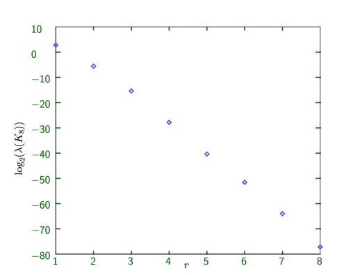
Figure 1: The eigenvalues of the Hankel matrix $K_{8}$.

2.4 Reduced order model (ROM)

In the rest of the paper, we let $\widetilde{\varphi}_{1},\widetilde{\varphi}_{2},\ldots,\widetilde{\varphi}_{r}$ be the order $r$ optimal reduced basis, which was generated in Algorithm 2, and we define $V_{r}$ by

$$V_{r}=\textup{span}\{\widetilde{\varphi}_{1},\widetilde{\varphi}_{2},\ldots,\widetilde{\varphi}_{r}\}.$$ (2.26)

Using the space $V_{r}$ we will construct the following two-steps backward differentiation reduced-order model (BDF2-ROM) scheme. Find $u_{r}^{n}\in V_{r}$ with $u_{r}^{0}=0$ satisfying

$$\left(\partial_{t}^{+}u_{r}^{n},v_{r}\right)+a\left(u_{r}^{n},v_{r}\right)=(f,v_{r}),\quad\forall v_{r}\in V_{r}.$$ (2.27)

Now, we are ready to compute the inner product in (2.27). Let $q_{j}$ be the $j$-th column of $Q$, then

$$A_{r,ij}=a(\widetilde{\varphi}_{j},\widetilde{\varphi}_{i})=\left(\sum_{m=1}^{N}(q_{j})_{m}\varphi_{m},\sum_{n=1}^{N}(q_{i})_{n}\varphi_{n}\right)_{V}=q_{j}^{\top}Aq_{i},$$

where $A$ is the stiffness matrix defined in (2.9). Hence,

$$A_{r}=\left[\begin{array}[]{cccc}q_{1}^{\top}Aq_{1}&q_{1}^{\top}Aq_{2}&\cdots&q_{1}^{\top}Aq_{r}\\[5.69046pt] q_{2}^{\top}Aq_{1}&q_{2}^{\top}Aq_{2}&\cdots&q_{2}^{\top}Aq_{r}\\ \vdots&\vdots&\cdots&\vdots\\ q_{r}^{\top}Aq_{1}&q_{r}^{\top}Aq_{2}&\cdots&q_{r}^{\top}Aq_{r}\\ \end{array}\right]=Q^{\top}AQ\in\mathbb{R}^{r\times r}.$$

Similarly, we define the reduced mass matrix and load vector.

$$M_{r}=Q^{\top}MQ\in\mathbb{R}^{r\times r},\quad\quad b_{r}=Q^{\top}b\in\mathbb{R}^{r}.$$ (2.28)

Finally, we are ready to complete the full implementation of (2.27). Since $u_{r}^{n}\in V_{r}$ holds, we make the Galerkin ansatz of the form

$$u_{r}^{n}=\sum_{j=1}^{r}\left(\alpha_{r}^{n}\right)_{j}{\widetilde{\varphi}}_{j}\quad\text{ for }n=1,2\ldots,N_{T}.$$ (2.29)

We insert (2.29) into (2.27) and have the following linear systems :

$$\begin{split}M_{r}\partial_{t}^{+}\alpha_{r}^{n}+A_{r}\alpha_{r}^{n}&=b_{r},\quad n\geq 1,\\ \alpha_{r}^{0}&\textit{}=0.\end{split}$$ (2.30)

For convenience, we should express the solution $u_{r}^{n}$ by using the standard finite element basis. By (2.15) and (2.29) we have

$$u_{r}^{n}=\sum_{j=1}^{r}\left(\alpha_{r}^{n}\right)_{j}{\widetilde{\varphi}}_{j}=\sum_{j=1}^{r}\left(\alpha_{r}^{n}\right)_{j}\sum_{i=1}^{N}(q_{j})_{i}\varphi_{i}=\sum_{i=1}^{N}(Q\alpha_{r}^{n})_{i}\varphi_{i}.$$

In other words, the coefficients of the solution $u_{r}^{n}$ in terms of the standard finite element basis are $Q\alpha_{n}$. It is worthwhile mentioning that to store the solution, we only need to save the matrix $Q\in\mathbb{R}^{N\times r}$ and the coefficient $\alpha_{n}\in\mathbb{R}^{r}$. Next, we summarize the above discussion in Algorithm 3.

Algorithm 3 (Fully implementation of (2.27))

Input: tol, $\ell$, $N_{T}$, $\Delta t$, $M$, $A$, $b$

1:$Q$ = GetTheMatrixQ$(\texttt{tol},\ell,M,A,b)$;                                                          % Algorithm 2

2:Set $M_{r}=Q^{\top}MQ$; $A_{r}=Q^{\top}AQ$; $b_{r}=Q^{\top}b$;

3:Solve $\left(\dfrac{1}{\Delta t}M_{r}+A_{r}\right)\alpha_{r}^{1}=b_{r}$;

4:for $n=2$ to $N_{T}$ do

5:     Solve $\left(\dfrac{3}{2\Delta t}M_{r}+A_{r}\right)\alpha_{r}^{n}=\dfrac{1}{\Delta t}M_{r}\left(2\alpha_{r}^{n-1}-\dfrac{1}{2}\alpha_{r}^{n-2}\right)+b_{r}$;

6:end for

7:return $Q,\alpha_{n}$

Example 3.

We revisit the Example 1 with the same problem data, mesh and time step. We choose $\ell=10$, tol $=10^{-14}$ in Algorithm 3. We report the dimension $r$ and the wall time of the ROM in Table 2. Comparing with Table 1, we see that our ROM is much faster than standard solvers. We also compute the $L^{2}$-norm error between the solutions of the FEM and the ROM at the final time $T=1$, we see that the error is close to the machine error. This motivated us that the solutions of the FEM and of the ROM are the same if we take tol small enough. In Section 3 we give a rigorous error analysis under an assumption on the source term $f$.

$h$								$1/2^{4}$	$1/2^{5}$	$1/2^{6}$	$1/2^{7}$	$1/2^{8}$	$1/2^{9}$	$1/2^{10}$
$r$	6	6	6	6	6	6	6
Wall time (s)	0.03	0.04	0.13	0.62	2.03	9.86	44.3
Error	6.73E-11	4.78E-15	2.03E-15	7.50E-14	6.87E-13	7.01E-13	7.88E-12

Table 2: Example 3: The dimension and wall time (seconds) of the ROM. The $L^{2}$-norm error between the solutions of the FEM and the ROM at the final time.

3 Error Analysis

Next, we provide a fully-discrete convergence analysis of the above new reduced order method for linear parabolic equations. Throughout the section, the constant $C$ depends on the polynomial degree $k$, the domain, the shape regularity of the mesh and the problem data. But, it does not depend on the mesh size $h$, the time step $\Delta t$ and the dimension of the ROM.

3.1 Main assumption and main result

First, we recall that $\Pi$ is the standard $L^{2}$ projection (see (2.21)) and $\{\phi_{j,h}\}_{j=1}^{N}$ are the eigenfuctions of (2.20) corresponding to the eigenvalues $\{\lambda_{j,h}\}_{j=1}^{N}$.

Next, we give our main assumptions in this section:

Assumption 1.

Low rank of $f$: there exist $\{c_{j}\}_{j=1}^{\ell}$ such that

$$\Pi f=\sum_{j=1}^{\ell}c_{j}\phi_{m_{j}h}.$$ (3.1)

Assumption 2.

The regularity of the solution of (2.2) is smooth enough.

Now, we state our main result in this section:

3.2 Sketch the proof of Theorem 2

To prove Theorem 2, we first bound the error between the solutions of the PDE (2.2) and FEM (2.4). Next we prove that the solutions of FEM (2.4) and the ROM (2.27) are exactly the same. Then we obtain a bound on the error between the solutions of PDE (2.2) and the ROM (2.27).

We begin by bounding the error between the solutions of the FEM (2.4) and PDE (2.2).

Lemma 7.

Let $u$ and $u_{h}^{n}$ be the solution of (2.2) and (2.4), respectively. If Assumption 2 holds, then we have

$$\left\|u(t_{n})-u_{h}^{n}\right\|\leq C\left(h^{k+1}+(\Delta t)^{2}\right).$$

The proof of Lemma 7 follows from standard estimates of finite element methods, therefore we skip it. Next, we prove that the solutions of FEM (2.4) and the ROM (2.27) are exactly the same.

Lemma 8.

Let $u_{h}^{n}$ be the solution of (2.4) and $u_{r}^{n}$ be the solution of (2.27) by setting tol$=0$ in Algorithm 3. If 1 holds, then for all $n=1,2,\ldots,N_{T}$ we have

$$u_{h}^{n}=u_{r}^{n}.$$

As a consequence, Lemmas 7 and 8 give the proof of Theorem 2.

3.3 Proof of Lemma 8

Since the eigenvalue problem (2.20) might have repeated eigenvalues, without loss of generality, we assume that only $\phi_{m_{1},h}$ and $\phi_{m_{2},h}$ share the same eigenvalues $\lambda_{m_{1},h}=\lambda_{m_{2},h}$. Recall that $\mu_{i}=1/\lambda_{i,h}$, then we have

$$\mu_{m_{1}}=\mu_{m_{2}}>\mu_{m_{3}}>\ldots>\mu_{m_{\ell}}.$$ (3.2)

By (2.17) we know that $\phi_{i,h}$ is the eigenfuntion of $\mathcal{A}_{h}^{-1}$ corresponding to the eigenvalue $\mu_{i}$. Now, we apply $\mathcal{A}_{h}^{-1}$, $\mathcal{A}_{h}^{-2}$, $\ldots$, $\mathcal{A}_{h}^{-\ell}$ to both sides of (3.1) to obtain:

$$\left[\begin{array}[]{cc}\mathfrak{u}_{h}^{1}\\[5.69046pt] \mathfrak{u}_{h}^{2}\\ \vdots\\ \mathfrak{u}_{h}^{\ell}\end{array}\right]=\left[\begin{array}[]{cccc}c_{1}\mu_{m_{1}}&c_{2}\mu_{m_{2}}&\cdots&c_{\ell}\mu_{m_{\ell}}\\[5.69046pt] c_{1}\mu_{m_{1}}^{2}&c_{2}\mu_{m_{2}}^{2}&\cdots&c_{\ell}\mu_{m_{\ell}}^{2}\\ \vdots&\vdots&\cdots&\vdots\\ c_{1}\mu_{m_{1}}^{\ell}&c_{2}\mu_{m_{2}}^{\ell}&\cdots&c_{\ell}\mu_{m_{\ell}}^{\ell}\end{array}\right]\left[\begin{array}[]{cc}\phi_{m_{1},h}\\[5.69046pt] \phi_{m_{2},h}\\ \vdots\\ \phi_{m_{\ell},h}\end{array}\right].$$ (3.15)

By the assumption (3.2), the rank of the coefficient matrix in (3.15) is $\ell-1$. Hence

$$\textup{span}\{\mathfrak{u}_{h}^{1},\mathfrak{u}_{h}^{2},\ldots,\mathfrak{u}_{h}^{\ell-1}\}=\textup{span}\{\mathfrak{u}_{h}^{1},\mathfrak{u}_{h}^{2},\ldots,\mathfrak{u}_{h}^{\ell}\}.$$

This implies that the matrix $K_{\ell-1}$ (see (2.13)) is positive definite and $K_{\ell}$ is positive semi-definite. Therefore, if we set tol$=0$ in the Algorithm 2, then the reduced basis space $V_{r}$ is given by

$$V_{r}=\textup{span}\{\widetilde{\varphi}_{1},\widetilde{\varphi}_{2},\ldots,\widetilde{\varphi}_{\ell-1}\}=\textup{span}\{\mathfrak{u}_{h}^{1},\mathfrak{u}_{h}^{2},\ldots,\mathfrak{u}_{h}^{\ell-1}\}.$$

Furthermore, by Lemma 1, for any $j=1,2,\ldots,\ell-1$ we have

$$\mathfrak{u}_{h}^{j}=\sum_{i=1}^{\ell-1}\left(\mathfrak{u}_{h}^{j},{\widetilde{\varphi}}_{i}\right)_{V}{\widetilde{\varphi}}_{i}.$$

For $i=1,2\ldots,\ell$, we define the sequence $\{\alpha_{i}^{n}\}_{n=1}^{N_{T}}$ by

$$\begin{split}\partial_{t}^{+}\alpha_{i}^{n}+\dfrac{1}{\mu_{m_{i}}}\alpha_{i}^{n}&=c_{i},\qquad n\geq 1,\\ \alpha_{i}^{0}&=0.\end{split}$$ (3.16)

Lemma 9.

If Assumption 1 holds, then the unique solution of (2.4) is given by

$$u_{h}^{n}=\sum_{i=1}^{\ell}\alpha_{i}^{n}\phi_{m_{i},h},\qquad n=1,2,\ldots,N_{T}.$$ (3.17)

Proof.

We only need to check that (3.17) satisfies (2.4). Substitute (3.17) into (2.4) we have

$$\left(\partial_{t}^{+}u_{h},v_{h}\right)+a\left(u_{h}^{n},v_{h}\right) =\left(\sum_{i=1}^{\ell}(\partial_{t}^{+}\alpha_{i}^{n})\phi_{m_{i},h},v_{h}\right)+a\left(\sum_{i=1}^{\ell}\alpha_{i}^{n}\phi_{m_{i},h},v_{h}\right)$$

$$=\left(\sum_{i=1}^{\ell}(\partial_{t}^{+}\alpha_{i}^{n})\phi_{m_{i},h},v_{h}\right)+\left(\sum_{i=1}^{\ell}\frac{\alpha_{i}^{n}}{\mu_{m_{i}}}\phi_{m_{i},h},v_{h}\right),$$

where we used the fact that $\phi_{m_{i},h}$ is the eigenvector of (2.20) corresponding to the eigenvalue $1/\mu_{m_{i}}$ in the last equality. Therefore, by (3.16) and Assumption 1 we have

$$\left(\partial_{t}^{+}u_{h},v_{h}\right)+a\left(u_{h}^{n},v_{h}\right)=\left(\sum_{i=1}^{\ell}c_{i}\phi_{m_{i},h},v_{h}\right)=(\Pi f,v_{h})=(f,v_{h}).$$

∎

Due to the assumption (3.2), it is easy to show that for all $n=1,2,\ldots,N_{T}$,

$$\alpha_{1}^{n}c_{2}=\alpha_{2}^{n}c_{1}.$$ (3.18)

Lemma 10.

Let $u_{h}^{n}$ be the solution of (2.4) and set tol$=0$ in Algorithm 3. If Assumption 1 and (3.2) hold, then for $n=1,2,\ldots,N_{T}$ we have

$$u_{h}^{n}\in V_{r}=\textup{span}\{\mathfrak{u}_{h}^{1},\mathfrak{u}_{h}^{2},\ldots,\mathfrak{u}_{h}^{\ell-1}\}.$$

Proof.

We rewrite the system (3.15) as

$$\left[\begin{array}[]{cc}\mathfrak{u}_{h}^{1}\\[5.69046pt] \mathfrak{u}_{h}^{2}\\ \vdots\\ \mathfrak{u}_{h}^{\ell-1}\end{array}\right]=\left[\begin{array}[]{cccc}c_{2}\mu_{m_{2}}&c_{3}\mu_{m_{3}}&\cdots&c_{\ell}\mu_{m_{\ell}}\\[5.69046pt] c_{2}\mu_{m_{2}}^{2}&c_{3}\mu_{m_{3}}^{2}&\cdots&c_{\ell}\mu_{m_{\ell}}^{2}\\ \vdots&\vdots&\cdots&\vdots\\ c_{2}\mu_{m_{2}}^{\ell-1}&c_{3}\mu_{m_{3}}^{\ell-1}&\cdots&c_{\ell}\mu_{m_{\ell}}^{\ell-1}\end{array}\right]\left[\begin{array}[]{cc}\phi_{m_{2},h}\\[5.69046pt] \phi_{m_{3},h}\\ \vdots\\ \phi_{m_{\ell},h}\end{array}\right]+\left[\begin{array}[]{cc}c_{1}\mu_{m_{1}}\\[5.69046pt] c_{1}\mu_{m_{1}}^{2}\\ \vdots\\ c_{1}\mu_{m_{1},h}^{\ell-1}\end{array}\right]\phi_{m_{1},h}.$$ (3.35)

We denote the coefficient matrix of (3.35) by $S$, it is obvious that $S$ is invertible since $\mu_{m_{2}}$, $\mu_{m_{3}}$, $\ldots$, $\mu_{m_{\ell}}$ are distinct. Furthermore, since $\mu_{m_{1}}=\mu_{m_{2}}$, then

$$S\left[\begin{array}[]{cc}1\\[5.69046pt] 0\\ \vdots\\ 0\end{array}\right]=\left[\begin{array}[]{cc}c_{2}\mu_{m_{2}}\\[5.69046pt] c_{2}\mu_{m_{2}}^{2}\\ \vdots\\ c_{2}\mu_{m_{2},h}^{\ell-1}\end{array}\right]=\left[\begin{array}[]{cc}c_{2}\mu_{m_{1}}\\[5.69046pt] c_{2}\mu_{m_{1}}^{2}\\ \vdots\\ c_{2}\mu_{m_{1},h}^{\ell-1}\end{array}\right].$$

This implies

$$\left[\begin{array}[]{cc}\phi_{m_{2},h}\\[5.69046pt] \phi_{m_{3},h}\\ \vdots\\ \phi_{m_{\ell},h}\end{array}\right]=S^{-1}\left[\begin{array}[]{cc}\mathfrak{u}_{h}^{1}\\[5.69046pt] \mathfrak{u}_{h}^{2}\\ \vdots\\ \mathfrak{u}_{h}^{\ell-1}\end{array}\right]-\dfrac{c_{1}}{c_{2}}\left[\begin{array}[]{cc}1\\[5.69046pt] 0\\ \vdots\\ 0\end{array}\right]\phi_{m_{1},h}.$$

Then by Lemma 9 and (3.18) we have

$$u_{h}^{n} =\sum_{i=1}^{\ell}\alpha_{i}^{n}\phi_{m_{i},h}=\alpha_{1}^{n}\phi_{m_{1},h}+\sum_{i=2}^{\ell}\alpha_{i}^{n}\phi_{m_{i},h}$$

$$=\alpha_{1}^{n}\phi_{m_{1},h}+\sum_{i=2}^{\ell}\alpha_{i}^{n}\sum_{j=1}^{\ell-1}S^{-1}_{i-1,j}\mathfrak{u}_{h}^{j}-\dfrac{c_{1}}{c_{2}}\alpha_{2}^{n}\phi_{m_{1},h}$$

$$=\sum_{i=2}^{\ell}\alpha_{i}^{n}\sum_{j=1}^{\ell-1}S^{-1}_{i-1,j}\mathfrak{u}_{h}^{j}.$$

This completes the proof.

∎

Proof of Lemma 8.

First, we take $v_{h}\in V_{r}\subset V_{h}$ in (2.4) to obtain

$$\left(\partial_{t}^{+}u_{h},v_{h}\right)+a\left(u_{h}^{n},v_{h}\right)=\left(\sum_{i=1}^{\ell}c_{i}\phi_{m_{i},h},v_{h}\right).$$ (3.36)

Subtract (3.36) from (2.27) and we let $e^{n}=u_{r}^{n}-u_{h}^{n}$, then

$$\left(\partial_{t}^{+}e^{n},v_{h}\right)+a\left(e^{n},v_{h}\right)=0.$$

By Lemma 10 we take $v_{h}=e^{n}\in V_{r}$ and the identity

$$(a-b,a) =\dfrac{1}{2}(\|a\|^{2}-\|b^{2}\|)+\dfrac{1}{2}\|a-b\|^{2},$$

$$\frac{1}{2}(3a-4b+c,a) =\frac{1}{4}\left[\|a\|^{2}+\|2a-b\|^{2}-\|b\|^{2}-\|2b-c\|^{2}\right]+\frac{1}{4}\|a-2b+c\|^{2},$$

to get

$$\|e^{1}\|^{2}-\|e^{0}\|^{2}+\left\|e^{1}-e^{0}\right\|^{2}+2\Delta t\left\|e^{1}\right\|_{V}^{2}=0.$$

Since $e^{0}=0$, then $e^{1}=0$. In other words

$$u_{r}^{1}=u_{h}^{1}.$$

For $n\geq 2$ we have

$$\left[\|e^{n}\|^{2}-\|e^{n-1}\|^{2}\right]+\left[\|2e^{n}-e^{n-1}\|^{2}-\|2e^{n-1}-e^{n-2}\|^{2}\right]+\|e^{n}-2e^{n-1}+e^{n-2}\|^{2}+4\Delta t\|e^{n}\|_{V}=0.$$

Summing both sides of the above identity from $n=2$ to $n=m$ completes the proof of Lemma 8. ∎

4 General data

In this section, we extend the new algorithm to more general cases. We assume that the source term $f$ can be expressed or approximated by a few only time dependent functions $f_{i}(t)$ and space dependent functions $g_{i}(x)$, i.e.,

$$f(t,x)=\sum_{i=1}^{m}f_{i}(t)g_{i}(x),$$

or

$$f(t,x)\approx\sum_{i=1}^{m}f(t_{i}^{*},x)L_{k,i}(t):=\sum_{i=1}^{m}f_{i}(t)g_{i}(x),$$

where $\{t_{i}^{*}\}_{i=1}^{m}$ are the $m$ Chebyshev interpolation nodes and $\{L_{m,i}(t)\}_{i=1}^{m}$ are the Lagrange interpolation functions:

$$t_{i}^{*} =\frac{T}{2}+\frac{T}{2}\cos\frac{(2i-1)\pi}{2m}\quad\textup{for}\quad i=1,2,\ldots,m,$$

$$L_{m,i}(t) =\frac{(t-t_{1}^{*})\cdots(t-t_{i-1}^{*})(t-t_{i+1}^{*})\cdots(t-t_{m}^{*})}{(t_{i}^{*}-t_{1}^{*})\cdots(t_{i}^{*}-t_{i-1}^{*})(t_{i}^{*}-t_{i+1}^{*})\cdots(t_{i}^{*}-t_{m}^{*})}.$$

Let $\{\varphi_{i}\}_{i=1}^{N}$ be the finite element basis function and we then define the following vectors:

$$b_{0}=[(u_{0},\varphi_{j})]_{j=1}^{N},\qquad b_{i}=[(g_{i},\varphi_{j})]_{j=1}^{N},\;\;i=1,2\ldots,m,\qquad B=[b_{0}\mid b_{1}\mid b_{2}\mid,\ldots,\mid b_{m}].$$ (4.1)

Algorithm 4

Input: tol, $\ell$, $M$, $A$, $B$

1:Solve $A\texttt{u}_{1}=B$;

2:for $i=2$ to $\ell$ do

3:     Solve $A\texttt{u}_{i}=M\texttt{u}_{i-1}$;

4:end for

5:Set $U=[\texttt{u}_{1}\mid\texttt{u}_{2}\mid\ldots\mid\texttt{u}_{\ell}]$;

6:Set $K=U^{\top}AU$;

7:$[\Psi,\Lambda]=\textup{eig}(K)$;

8:Find minimal $r$ such that $\sum_{k=1}^{r}{\Lambda(k,k)}/{\sum_{k=1}^{(i+1)\ell}\Lambda(k,k)}\geq 1-\textup{tol}$;

9:Set $Y=U\Psi(:,1:r)(\Lambda(1:r;1:r))^{-1/2}$;

10:return $Y$

By the linearity, one trivial idea is to apply Algorithm 3 $m+1$ times. This can be computationally expensive if $m$ is not small. Following an ensemble idea in [6], we can treat $\{b_{i}\}_{i=0}^{m}$ simultaneously (see Algorithm 4) since these linear systems share a common coefficient matrix; it is more efficient than solving the linear system with a single RHS for $m+1$ times.

Unfortunately, a downside of this approach is a loss of numerical precision. More precisely, the convergence rates are not stable when the mesh size $h$ and time step $\Delta t$ are small, or when the error is pretty small; see Table 3. This is possibly due to the fast decay of the eigenvalues of $K$. To resolve the problem, we use the singular values of $U$ as the stopping criteria. We see that the convergence is very stable; see Table 5.

We note that the standard singular value decomposition (SVD) of $U$ is not equivalent to the eigen decomposition of $K$. In [8], the authors showed that the output of Algorithm 4, $Y$, is the first $r$ columns of $Q$ in the following Definition 1.

Definition 1.

[8] A core SVD of a matrix $U\in\mathbb{R}^{N\times n}$ is a decomposition $U=Q\Sigma R^{\top}$, where $Q\in\mathbb{R}^{N\times d},\Sigma\in\mathbb{R}^{d\times d}$, and $R\in\mathbb{R}^{n\times d}$ satisfy

$$Q^{\top}AQ=I,\quad R^{\top}R=I,\quad\Sigma=\operatorname{diag}\left(\sigma_{1},\ldots,\sigma_{d}\right),$$

where $\sigma_{1}\geq\sigma_{2}\geq\cdots\geq\sigma_{d}>0$. The values $\left\{\sigma_{i}\right\}$ are called the (positive) singular values of $U$ and the columns of $Q$ and $R$ are called the corresponding singular vectors of $U$.

Next, we introduce an efficient method to compute the core SVD of $U$.

4.1 Incremental SVD

Incremental SVD was proposed by Brand in [4], the algorithm updates the SVD of a matrix when one or more columns are added to the matrix. However, if we directly apply Brand’s algorithm to compute the core SVD of $U$, we have to compute the Cholesky factorization of the weighted matrix $A$. Recently, Fareed et al. [8] modified Brand’s algorithm in a weighted norm setting without computing the Cholesky factorization of $A$.

Next we briefly discuss the main idea of the algorithm.

Suppose we already have the rank-$k$ truncated core SVD of $U_{i}$ (the first $i$ columns of $U$):

$$U_{i}=Q\Sigma R^{\top},\quad\textup{with}\;\;Q^{\top}AQ=I,\quad R^{\top}R=I,\quad\Sigma=\operatorname{diag}\left(\sigma_{1},\ldots,\sigma_{k}\right),$$ (4.2)

where $\Sigma\in\mathbb{R}^{k\times k}$ is a diagonal matrix with the $k$ (ordered) singular values of $U_{i}$ on the diagonal, $Q\in\mathbb{R}^{N\times k}$ is the matrix containing the corresponding $k$ left singular vectors of $U_{i}$, and $R\in\mathbb{R}^{i\times k}$ is the matrix of the corresponding $k$ right singular vectors of $U_{i}$.

The main idea of Brand’s algorithm is to update the matrix $U_{i+1}:=\left[\begin{array}[]{ll}U_{i}&u_{i+1}\end{array}\right]$ by using the SVD of $U_{i}$ and the new coming data $u_{i+1}$. Set $p=\|u_{i+1}-QQ^{\top}Au_{i+1}\|_{A}$, where $\|x\|_{A}^{2}=x^{\top}Ax$. Then the incremental SVD algorithm arises from the following fundamental identity:

Then the SVD of $U_{i+1}$ can be constructed by

• finding the full SVD of $\left[\begin{array}[]{cc}\Sigma&Q^{\top}Au_{i+1}\\ 0&p\end{array}\right]=\widetilde{Q}\widetilde{\Sigma}\widetilde{R}^{\top}$, and then

• updating the SVD of $U_{i+1}$ by

  $$U_{i+1}=\left(\left[\begin{array}[]{ll}Q&(I-QQ^{\top}A)u_{i+1}/p\end{array}\right]\widetilde{Q}\right)\widetilde{\Sigma}\left(\left[\begin{array}[]{cc}R&0\\ 0&1\end{array}\right]\widetilde{R}\right)^{\top}.$$

In practice, small numerical errors cause a loss of orthogonality, hence reorthogonalizations are needed and the computational cost can be high. Very recently, Zhang [30] proposed an efficient way to reduce the complexity; see [30, Section 4.2] for more details.

Now we apply the new incremental SVD algorithm in [30] to find the core SVD of the matrix $U$ in Algorithm 4. Obviously, the main computational cost is to solve the matrix equations for $\ell$ times. Although solving a linear system with multiple RHS is more efficient than solving multiple linear systems with a single RHS, it is still expensive if we have a large amount of RHS. To reduce the computational cost, we find a low rank approximation of the matrix $B$ in (4.1).

Let $B=Q_{F}\Sigma_{F}R_{F}^{\top}$ be a thin SVD of $B$, the number of the columns of $Q_{F}$ is small if the data is low rank or approximately low rank. We summarize the above discussions in Algorithm 5.

Algorithm 5

Input: $M\in\mathbb{R}^{N\times N}$, $A\in\mathbb{R}^{N\times N}$, $\{b_{i}\}_{i=0}^{m}$, tol

1:$[Q_{F},\Sigma_{F},R_{F}]=$ svd$(B$, ‘econ’);

2:Find the minimal $p$ such that $\Sigma_{F}(p+1,p+1)\leq\texttt{tol}$;

3:Let $Q_{p}$ be the first $p$ columns of $Q_{F}$;

4:Solve $A\texttt{U}_{1}=Q_{p}$;

5:$Q=[]$, $\Sigma=[]$, $R=[]$;

6:$[Q,\Sigma,R]=$ Fullisvd($Q,\Sigma,R,A$, $\texttt{U}_{1}$, tol);                                % [30, Algorithm 9]

7:for $i=2$ to $\ell$ do

8:     Solve $A\texttt{U}_{i}=M\texttt{U}_{i-1}$;

9:     $[Q,\Sigma,R]=$ Fullisvd($Q,\Sigma,R,A$, $\texttt{U}_{i}$, tol);                            % [30, Algorithm 9]

10:end for

11:return $Q$, $Q_{F}$, $\Sigma_{F}$, $R_{F}$

4.2 ROM

Let $r$ be the number of the column of $Q$ in Algorithm 5, and define $V_{r}$ by

$$V_{r}=\textup{span}\{\widetilde{\varphi}_{1},\widetilde{\varphi}_{2},\ldots,\widetilde{\varphi}_{r}\},\quad\textup{with}\quad\widetilde{\varphi}_{j}=\sum_{k=1}^{N}Q(k,j)\varphi_{k},\quad\textup{for }j=1,2\cdots,r.$$ (4.4)

We are looking for a function $u_{r}(t)\in C((0,T];V_{r})$ satisfying

$$\begin{split}\frac{\mathrm{d}}{\mathrm{d}t}(u_{r}(t),v_{h})+a(u_{r}(t),v_{h})&=(f,v_{h})\qquad\qquad\;\;\;\;\forall v_{h}\in V_{r},\\ (u_{r}(0),v_{h})&=(u_{0},v_{h})\quad\quad\quad\quad\quad\forall v_{h}\in V_{r}.\end{split}$$ (4.5)

Since $u_{r}(t)\in V_{r}$ holds, we make the Galerkin ansatz of the form

$$u_{r}(t)=\sum_{j=1}^{r}u_{j}^{r}(t)\widetilde{\varphi}_{j}.$$ (4.6)

We insert (4.6) into (4.5) and define the modal coefficient vector

$$U_{r}(t)=\left(u_{j}^{r}(t)\right)_{1\leq j\leq r}\quad\text{ for }t\in[0,T].$$

From (4.5) we derive the linear system of ordinary differential equations

$$\begin{split}M_{r}{U}^{\prime}_{r}(t)+A_{r}U_{r}(t)&=\sum_{i=1}^{m}f_{i}(t)b_{i}^{r}\quad t\in(0,T],\\ U_{r}(0)&=b_{0}^{r}.\end{split}$$ (4.7)

where

$$M_{r}=Q^{\top}MQ\in\mathbb{R}^{r\times r},\;\;A_{r}=Q^{\top}AQ\in\mathbb{R}^{r\times r},\;\;b_{i}^{r}=Q^{\top}b_{i}\in\mathbb{R}^{r},i=0,1,2,\ldots,k.$$

Note that (4.7) can then be solved by using an appropriate method for the time discretization.

4.3 Numerical experiments

In this section, we present several numerical tests to show the accuracy and efficiency of our new method. In all examples, we let $\Omega=(0,1)^{2}$ in 2D and $\Omega=(0,1)^{3}$ in 3D and final time $T=1$. The source term $f$ is chosen so that the exact solution is

$$u=\begin{cases}\sin(t)\cos(tx)x\sin(x-1)\sin(y)(y-1)&\textup{in}\;\;2D,\\ \sin(t)\cos(tx)x\sin(x-1)\sin(y)(y-1)\sin(z)(z-1)&\textup{in}\;\;3D.\end{cases}$$

First, we choose $\ell=5,m=8$, $\texttt{tol}=10^{-10}$ and apply Algorithm 4 to get the ROM (4.7), then we use the backward Euler for the first step and then apply the two-steps backward differentiation formula (BDF2) for the time discretization and take time step $\Delta t=h^{(k+1)/2}$, here $h$ is the mesh size and $k$ is the polynomial degree. We report the error at the final time $T=1$ and wall time in Table 3. We see that the convergence rate of the ROM is the same as the standard finite element method when $k=1$. However, the convergence rates are not stable due to a loss of numerical precision; see the case of $k=2$ in Table 3.

Degree	$\frac{h}{\sqrt{2}}$	Wall time (s)	$\|u-u_{r}\|_{L^{2}(\Omega)}$		$\|\nabla(u-u_{r})\|_{L^{2}(\Omega)}$
			Error	Rate	Error	Rate
$k=1$	$2^{-3}$	0.1876	9.3278E-04	-	1.9653E-02	-
	$2^{-4}$	0.0570	2.3677E-04	1.98	9.8978E-03	0.99
	$2^{-5}$	0.0922	5.9423E-05	1.99	4.9579E-03	1.00
	$2^{-6}$	0.2523	1.4873E-05	2.00	2.4801E-03	1.00
	$2^{-7}$	1.0610	3.7233E-06	2.00	1.2402E-03	1.00
$k=2$	$2^{-3}$	0.1552	2.3143E-05	-	1.4701E-03	-
	$2^{-4}$	0.0943	2.8966E-06	3.00	3.7004E-04	1.99
	$2^{-5}$	0.2106	3.7517E-07	2.95	9.2685E-05	2.00
	$2^{-6}$	0.7487	1.0784E-07	1.80	2.3222E-05	2.00
	$2^{-7}$	3.4102	9.7986E-08	0.14	5.9637E-06	1.96

Table 3: Algorithm 4: 2D: The errors for $u_{r}$ and $\nabla u_{r}$ at the final time $T=1$.

Second, we test the efficiency and accuracy of Algorithm 5 under the same problem data and setting as above. We report the error at the final time $T=1$ and wall time in Tables 4 and 5. We see that the convergence rate of the ROM is the same as the standard finite element method.

Degree	$\frac{h}{\sqrt{2}}$	Wall time (s)	$\|u-u_{r}\|_{L^{2}(\Omega)}$		$\|\nabla(u-u_{r})\|_{L^{2}(\Omega)}$
			Error	Rate	Error	Rate
$k=1$	$2^{-3}$	0.1438	9.3549E-04	-	1.9653E-02	-
	$2^{-4}$	0.0473	2.3727E-04	1.98	9.8978E-03	0.99
	$2^{-5}$	0.0779	5.9521E-05	2.00	4.9579E-03	1.00
	$2^{-6}$	0.2351	1.4891E-05	2.00	2.4801E-03	1.00
	$2^{-7}$	1.0067	3.7232E-06	2.00	1.2402E-03	1.00
$k=2$	$2^{-3}$	0.1893	2.3208E-05	-	1.4701E-03	-
	$2^{-4}$	0.1027	2.8977E-06	3.00	3.7004E-04	1.99
	$2^{-5}$	0.2585	3.6209E-07	3.00	9.2674E-05	2.00
	$2^{-6}$	0.8738	4.5252E-08	3.00	2.3179E-05	2.00
	$2^{-7}$	3.8290	5.6561E-09	3.00	5.7954E-06	2.00

Table 4: Algorithm 5: 2D: The errors for $u_{r}$ and $\nabla u_{r}$ at the final time $T=1$.

Degree	$\frac{h}{\sqrt{2}}$	Wall time (s)	$\|u-u_{r}\|_{L^{2}(\Omega)}$		$\|\nabla(u-u_{r})\|_{L^{2}(\Omega)}$
			Error	Rate	Error	Rate
$k=1$	$2^{-2}$	0.2370	9.5386E-04	-	1.0151E-02	-
	$2^{-3}$	0.2663	2.6633E-04	1.84	5.3315E-03	0.93
	$2^{-4}$	2.8694	6.8562E-05	1.96	2.7000E-03	0.98
	$2^{-5}$	15.693	1.7269E-05	1.99	1.3544E-03	1.00
	$2^{-6}$	145.73	4.3254E-06	2.00	6.7774E-04	1.00
$k=2$	$2^{-2}$	0.3842	2.3139E-05	-	1.4701E-03	-
	$2^{-3}$	1.8871	7.3028E-06	3.00	4.9435e-04	1.99
	$2^{-4}$	11.790	9.0664E-07	3.00	1.2573E-04	2.00
	$2^{-5}$	120.47	1.1318E-07	3.00	3.1585E-05	2.00
	$2^{-6}$	1294.7	1.4144E-08	3.00	7.9064E-06	2.00

Table 5: Algorithm 5: 3D: The errors for $u_{r}$ and $\nabla u_{r}$ at the final time $T=1$.

5 Conclusion

In the paper, we proposed a new reduced order model (ROM) of linear parabolic PDEs. We proved that the singular values of the Krylov sequence are exponential decaying (Theorem 1). Furthermore, under some assumptions, we proved that the solutions of the ROM and the FEM have the same convergence rates (Theorem 2). There are many interesting directions for the future research. First, we will investigate the non-homogeneous Dirichlet boundary conditions and the corresponding Dirichlet boundary control problems, such as [13, 12, 16, 7, 11]. Second, we will consider the ROM for hyperbolic PDEs and Maxwell’s equations [22, 21]. Third, we will apply our result for realistic problems, such as inverse problems, shape optimization problems and data assimilation problems. Our long term goal is to build accurate ROMs for nonlinear PDEs.

References

- [1] F. Bai and Y. Wang, Deim reduced order model constructed by hybrid snapshot simulation, SN Applied Sciences, 2 (2020), pp. 1–25.
- [2] B. Beckermann and A. Townsend, Bounds on the singular values of matrices with displacement structure, SIAM Rev., 61 (2019), pp. 319–344, https://doi.org/10.1137/19M1244433. Revised reprint of “On the singular values of matrices with displacement structure” [ MR3717820].
- [3] P. Benner, S. Gugercin, and K. Willcox, A survey of projection-based model reduction methods for parametric dynamical systems, SIAM Rev., 57 (2015), pp. 483–531, https://doi.org/10.1137/130932715.
- [4] M. Brand, Incremental singular value decomposition of uncertain data with missing values, in European Conference on Computer Vision, Springer, 2002, pp. 707–720.
- [5] D. Chapelle, A. Gariah, P. Moireau, and J. Sainte-Marie, A Galerkin strategy with proper orthogonal decomposition for parameter-dependent problems—analysis, assessments and applications to parameter estimation, ESAIM Math. Model. Numer. Anal., 47 (2013), pp. 1821–1843, https://doi.org/10.1051/m2an/2013090.
- [6] G. Chen, L. Pi, L. Xu, and Y. Zhang, A superconvergent ensemble HDG method for parameterized convection diffusion equations, SIAM J. Numer. Anal., 57 (2019), pp. 2551–2578, https://doi.org/10.1137/18M1192573.
- [7] G. Chen, J. R. Singler, and Y. Zhang, An HDG method for Dirichlet boundary control of convection dominated diffusion PDEs, SIAM J. Numer. Anal., 57 (2019), pp. 1919–1946, https://doi.org/10.1137/18M1208708.
- [8] H. Fareed, J. R. Singler, Y. Zhang, and J. Shen, Incremental proper orthogonal decomposition for PDE simulation data, Comput. Math. Appl., 75 (2018), pp. 1942–1960, https://doi.org/10.1016/j.camwa.2017.09.012.
- [9] D. Fasino and G. Inglese, On the spectral condition of rectangular Vandermonde matrices, Calcolo, 29 (1992), pp. 291–300 (1993), https://doi.org/10.1007/BF02576186.
- [10] X. Fu and J. N. Kutz, Adaptive dimensionality-reduction for time-stepping in differential and partial differential equations, Numer. Math. Theory Methods Appl., 10 (2017), pp. 872–894, https://doi.org/10.4208/nmtma.2017.m1624.
- [11] W. Gong, W. Hu, M. Mateos, J. Singler, X. Zhang, and Y. Zhang, A new HDG method for Dirichlet boundary control of convection diffusion PDEs II: low regularity, SIAM J. Numer. Anal., 56 (2018), pp. 2262–2287, https://doi.org/10.1137/17M1152103.
- [12] W. Gong, W. Hu, M. Mateos, J. R. Singler, and Y. Zhang, Analysis of a hybridizable discontinuous Galerkin scheme for the tangential control of the Stokes system, ESAIM Math. Model. Numer. Anal., 54 (2020), pp. 2229–2264, https://doi.org/10.1051/m2an/2020015.
- [13] W. Gong, M. Mateos, J. Singler, and Y. Zhang, Analysis and approximations of Dirichlet boundary control of Stokes flows in the energy space, SIAM J. Numer. Anal., 60 (2022), pp. 450–474, https://doi.org/10.1137/21M1406799, https://doi.org/10.1137/21M1406799.
- [14] M. Gubisch and S. Volkwein, Proper orthogonal decomposition for linear-quadratic optimal control, Model reduction and approximation: theory and algorithms, 15 (2017).
- [15] C. Homescu, L. R. Petzold, and R. Serban, Error estimation for reduced-order models of dynamical systems, SIAM Rev., 49 (2007), pp. 277–299, https://doi.org/10.1137/070684392.
- [16] W. Hu, J. Shen, J. R. Singler, Y. Zhang, and X. Zheng, A superconvergent hybridizable discontinuous Galerkin method for Dirichlet boundary control of elliptic PDEs, Numer. Math., 144 (2020), pp. 375–411, https://doi.org/10.1007/s00211-019-01090-2.
- [17] B. Koc, S. Rubino, M. Schneier, J. Singler, and T. Iliescu, On optimal pointwise in time error bounds and difference quotients for the proper orthogonal decomposition, SIAM J. Numer. Anal., 59 (2021), pp. 2163–2196, https://doi.org/10.1137/20M1371798.
- [18] K. Kunisch and S. Volkwein, Galerkin proper orthogonal decomposition methods for parabolic problems, Numer. Math., 90 (2001), pp. 117–148, https://doi.org/10.1007/s002110100282.
- [19] K. Kunisch and S. Volkwein, Galerkin proper orthogonal decomposition methods for a general equation in fluid dynamics, SIAM J. Numer. Anal., 40 (2002), pp. 492–515, https://doi.org/10.1137/S0036142900382612.
- [20] S. Locke and J. Singler, New proper orthogonal decomposition approximation theory for PDE solution data, SIAM J. Numer. Anal., 58 (2020), pp. 3251–3285, https://doi.org/10.1137/19M1297002.
- [21] P. Monk, Finite element methods for Maxwell’s equations, Numerical Mathematics and Scientific Computation, Oxford University Press, New York, 2003, https://doi.org/10.1093/acprof:oso/9780198508885.001.0001.
- [22] P. Monk and Y. Zhang, Finite element methods for maxwell’s equations, (2019).
- [23] M.-L. Rapún and J. M. Vega, Reduced order models based on local POD plus Galerkin projection, J. Comput. Phys., 229 (2010), pp. 3046–3063, https://doi.org/10.1016/j.jcp.2009.12.029.
- [24] J. W. Ruge and K. Stüben, Algebraic multigrid, in Multigrid methods, vol. 3 of Frontiers Appl. Math., SIAM, Philadelphia, PA, 1987, pp. 73–130.
- [25] J. Shen, J. R. Singler, and Y. Zhang, HDG-POD reduced order model of the heat equation, J. Comput. Appl. Math., 362 (2019), pp. 663–679, https://doi.org/10.1016/j.cam.2018.09.031.
- [26] J. R. Singler, New POD error expressions, error bounds, and asymptotic results for reduced order models of parabolic PDEs, SIAM J. Numer. Anal., 52 (2014), pp. 852–876, https://doi.org/10.1137/120886947.
- [27] G. Talenti, Recovering a function from a finite number of moments, Inverse Problems, 3 (1987), pp. 501–517.
- [28] F. Terragni, E. Valero, and J. M. Vega, Local POD plus Galerkin projection in the unsteady lid-driven cavity problem, SIAM J. Sci. Comput., 33 (2011), pp. 3538–3561, https://doi.org/10.1137/100816006.
- [29] H. S. Wilf, Finite sections of some classical inequalities, Ergebnisse der Mathematik und ihrer Grenzgebiete, Band 52, Springer-Verlag, New York-Berlin, 1970.
- [30] Y. Zhang, An answer to an open question in the incremental SVD, https://doi.org/https://arxiv.org/abs/2204.05398.