Leveraging GPU Tensor Cores for Double Precision Euclidean Distance Calculations

Abstract

Tensor cores (TCs) are a type of Application-Specific Integrated Circuit (ASIC) and are a recent addition to Graphics Processing Unit (GPU) architectures. As such, TCs are purposefully designed to greatly improve the performance of Matrix Multiply-Accumulate (MMA) operations. While TCs are heavily studied for machine learning and closely related fields, where their high efficiency is undeniable, MMA operations are not unique to these fields. More generally, any computation that can be expressed as MMA operations can leverage TCs, and potentially benefit from their higher computational throughput compared to other general-purpose cores, such as CUDA cores on Nvidia GPUs. In this paper, we propose the first double precision (FP64) Euclidean distance calculation algorithm, which is expressed as MMA operations to leverage TCs on Nvidia GPUs, rather than the more commonly used CUDA cores. To show that the Euclidean distance can be accelerated in a real-world application, we evaluate our proposed TC algorithm on the distance similarity self-join problem, as the most computationally intensive part of the algorithm consists of computing distances in a multi-dimensional space. We find that the performance gain from using the tensor core algorithm over the CUDA core algorithm depends weakly on the dataset size and distribution, but is strongly dependent on data dimensionality. Overall, TCs are a compelling alternative to CUDA cores, particularly when the data dimensionality is low ($\leq{4}$), as we achieve an average speedup of $1.28\times$ and up to $2.23\times$ against a state-of-the-art GPU distance similarity self-join algorithm. Furthermore, because this paper is among the first to explore the use of TCs for FP64 general-purpose computation, future research is promising.

I Introduction

Tensor cores (TCs) are a type of Application-Specific Integrated Circuit (ASIC), and are specifically designed for Matrix Multiply-Accumulate (MMA) operations. The high specificity of TCs makes them typically more efficient at computing MMA operations, than other more general-purpose cores such as CPU cores or GPU CUDA cores. Given four matrices $A,B,C$, and $D$, TCs are designed to compute $D=A\times B+C$ (where $C$ and $D$ may be the same matrix). Over the past few years, TCs have been heavily used for machine learning and other fields requiring linear algebra, and few papers have examined broadening the use of TCs for other algorithms. Despite their high specificity, TCs may also be very versatile: any computation expressed with MMA operations, as defined above, should be able to leverage TCs and consequently, benefit from their high computational throughput.

Several companies have proposed a version of TCs, each with its own different characteristics. In this paper, we focus on the Nvidia GPU TCs. These TCs were first introduced with the Volta generation in 2017. Since this first iteration, they have been implemented in several GPU models and have greatly improved over time [1, 2, 3]. In particular, while the first generation of TCs was only capable of computing in half precision using 16-bit floats (FP16), TCs are now capable of double precision computing using 64-bit floats (FP64) with the Ampere generation [2]. This enables TCs to be used for applications where high precision is critical. Furthermore, their number, as well as their theoretical computational throughput, have continued to increase, making them an attractive alternative to the general-purpose CUDA cores.

As mentioned above, in this paper we focus on TCs proposed by Nvidia on their GPUs. In addition to the CUDA API to access GPU functionalities, we also leverage the Warp Matrix Multiply-Accumulate (WMMA) API [4, 5], which provides programmatic access to TCs. While other libraries also give access to TCs, they are all higher level than the WMMA API and less versatile, thus less suited to our use case. However, there are some limitations when using the WMMA API. In particular, matrix sizes are limited to a few options, and not all compute precisions are available or can be combined (e.g., FP32 for both multiplication and accumulation is not available, and FP16 multiplication can not be combined with FP64 accumulation).

The Euclidean distance is a metric commonly used in many scientific applications, particularly for data analysis algorithms such as the distance similarity self-join [6, 7, 8, 9], the $k$NN [10], or the Density-Based Spatial Clustering of Applications with Noise (DBSCAN) [11] algorithms. Within these algorithms, distance calculations are usually the most time-consuming fraction of the total computation [12]. In this paper, we propose to improve the throughput of Euclidean distance calculations by leveraging TCs on the GPU, and consequently also improve the overall performance of the algorithms mentioned above. To illustrate greater applicability to these other algorithms, we use the distance similarity self-join algorithm as a representative example case for the other data analysis algorithms mentioned above. Given a dataset $V$ in $d$ dimensions, the distance similarity self-join algorithm finds all pairs of points $(a,b)$ that are within a distance threshold $\epsilon$ of each other; $dist(a,b)\leq\epsilon$, where $a,b\in V$, and dist is the Euclidean distance function.

This paper makes the following contributions:

•We propose a new algorithm for computing Euclidean distances using TCs, leveraging the Nvidia Ampere architecture TCs [2] supporting double precision (FP64) computations.

•We integrate the aforementioned method into the distance similarity self-join algorithm, that we name Tensor Euclidean Distance Join (TED-Join). We show that TED-Join is competitive with the best parallel distance similarity self-joins in the literature for multi-core CPUs and GPU CUDA cores.

•The solution we propose here extends beyond the distance similarity self-join algorithm and can be integrated into other algorithms that use the distance similarity self-join, or more generally Euclidean distance calculations, as a building block.

•We evaluate TED-Join across a broad range of datasets, that span several distributions, sizes and dimensionalities, and compare it to a state-of-the-art GPU CUDA cores (GDS-Join [6]) and two multi-core CPU distance similarity join algorithms, Super-EGO [7] and FGF-Hilbert [8]. We conclude that TED-Join should always be preferred over Super-EGO and FGF-Hilbert, and should be preferred over GDS-Join when the dimensionality $d\leq 4$, where it achieves an average speedup of $1.28\times$ (and $1.07\times$ when considering all the experiments we conducted), and up to $2.23\times$.

•To our knowledge, this paper proposes the first Euclidean distance calculation for TCs using FP64 computation, and the first use of TCs for the distance similarity self-join.

The paper is outlined as follows: we present essential material in Section II, including an overview of TCs. We then present in Section III our solution that uses TCs to compute Euclidean distances and its integration into the distance similarity self-join algorithm. We show in Section IV the performance of our solution compared to the state-of-the-art distance similarity self-join algorithms, and we conclude and propose future research directions in Section V.

II Background

II-A Problem Statement

For two points $a$ and $b$ in $d$ dimensions, and where $a_{i}$ represents the $i^{th}$ coordinate of the point $a$, and where $i=1,\ldots,d$, the Euclidean distance between $a$ and $b$ is defined as follows:

$$dist(a,b)=\sqrt{\sum^{d}_{i=1}(a_{i}-b_{i})^{2}}.$$ (1)

The distance similarity self-join algorithm, as described above, takes a dataset $V$ in $d$ dimensions as well as a search distance $\epsilon$ as inputs, and finds all the pairs of points $(a,b)$ such that $dist(a,b)\leq\epsilon$ where $a,b\in V$, and where the distance function is, in this case, the Euclidean distance defined in Equation 1. For a query point $a$, finding all the other points in $V$ within $\epsilon$ from $a$ is called a range query ($|V|$ range queries in total).

II-B Tensor Cores (TCs)

TCs on GPUs are an Application-Specific Integrated Circuit (ASIC) designed for Matrix Multiply-Accumulate (MMA) operations. Given four matrices $A,B,C$ and $D$, this MMA operation is expressed as $D=A\times B+C$. Matrices $C$ and $D$ are the accumulators and may be equivalent. In hardware, TCs are designed to process $4\times 4$ MMA operations. However, the WMMA API only gives access to larger matrices (e.g., $16\times 16$). Therefore, several TCs are used concurrently to perform MMA operations larger than $4\times 4$. Due to their highly specific design, TCs are significantly more efficient at MMA operations than CUDA cores: double precision computation is presented as twice as efficient when using TCs compared to CUDA cores on the Nvidia A100 GPU [2]. This significantly higher processing throughput is our motivation to transform Euclidean distance calculation into MMA operations, and yield higher computational throughput.

The WMMA API [4, 5] provides some low-level access to TCs, giving us the highest versatility possible. However, several limitations come along with this WMMA API. In particular, it is limited to certain matrix sizes and compute precisions. Among the options available, only a few are relevant to our work. In this paper, we focus on FP64 computation, which limits us to only one size for each of our matrices. Let $M_{m,n}$ be a matrix with $m$ rows and $n$ columns. The matrices that we can use with double precision are thus $A_{8,4}$, $B_{4,8}$, $C_{8,8}$, and $D_{8,8}$. We refer the reader to the documentation [4] for the other TCs options.

Programmatically, the matrices proposed by the WMMA API are called fragments, and are stored into the GPU threads registers. The WMMA API defines several functions:

•load_matrix_sync(): Load a matrix fragment from memory.

•store_matrix_sync(): Store a matrix fragment into memory.

•mma_sync(): Perform an MMA operation using TCs.

•fill_fragment(): Fill a matrix fragment with a specified value.

As their name suggests, these function calls are synchronized. Hence, all 32 threads of the warp are blocked until the operation is complete. The load and store functions take, among other arguments, a stride between the elements comprising the matrix rows. Hence, all the elements consisting of a row in the target matrix need to be coalesced in memory. Furthermore, the individual elements of the matrix fragments are stored in an unspecified order in the registers. Thus, contrary to regular arrays, the first element of a matrix may not be stored in the first element of the fragment. Consequently, operations on an individual element of a matrix fragment need to be applied to all the other elements, using a loop iterating over all of the elements of the fragment.

II-C Tensor Cores in the Literature

As mentioned above, the literature concerning TCs heavily revolves around machine learning and other closely related fields, and not many other types of applications employing TCs [13, 14, 15, 16, 17]. We present in this section a selection of papers that discuss the use of TCs for applications that focus more on computational/data-enabled science, similarly to this paper. Moreover, since most of the literature seems to focus on low precision computations, we believe that this paper is the first to propose an implementation using TCs for FP64 computations.

Dakkak et al. [13] propose a method to perform reduction and scan operations, using the WMMA API to leverage TCs. Their reduction algorithm consists of multiplying a matrix whose first row are ones and the rest are zeros with a matrix containing the values to reduce, and accumulated with a matrix containing the result from previous reductions. Their scan solution is similar but uses an upper triangular matrix filled with ones and where the rest are zeros, instead of a single row filled with ones. Their proposed solutions achieve a speedup of $100\times$ for the reduction and $3\times$ for the scan, compared to other state-of-the-art methods not using TCs.

Ji and Wang [14] propose using TCs to improve the performance of the DBSCAN algorithm. They mainly use TCs to compute distance matrices between the points that might form a cluster, using the cosine similarity formula (in contrast to the Euclidean distance used in this paper). They also use TCs to perform reductions, which are used to determine if points belong to a cluster or not. Their solution using TCs achieves a speedup of up to $2.61\times$ to compute distance matrices compared to using the CUDA cores. While this work is very relevant to us, it differs in that they use a different distance metric (cosine similarity vs. Euclidean distance), they do not use an index structure, and part of their work is exclusive to the DBSCAN algorithm. In comparison, our solution essentially concerns the Euclidean distance calculations and, therefore, more applications than the distance similarity self-join that we just take as an example for this paper.

Ahle and Silvestri [15] theorize using TCs to compute similarity searches. They use TCs to compute either the Hamming, squared $L_{2}$ distances, or cosine similarity through an inner product operation, expressed as matrix multiplications. Additionally, they opt for the Local Sensitivity Hashing (LSH) method, reducing the overall complexity of the computation similarly to an indexing structure used by other similarity join solutions [7, 8, 6]. However, and contrary to these solutions, the LSH method typically yields an approximate result.

II-D Distance Similarity Joins

We discuss in this section several state-of-the-art parallel distance similarity self-join algorithms [6, 7, 9, 8], which we use as reference implementations for our experimental evaluation. These selected algorithms have in common that they use an indexing structure to prune the number of distance calculations, which is a commonly used optimization [18, 19]. When using an index, it is first searched to yield a set of candidate points for each query point. The set of candidate points is then refined using distance calculations to keep pairs of query and candidate points that are within $\epsilon$ of each other.

Kalashnikov [7] proposes Super-EGO, a parallel CPU algorithm to compute a distance similarity join, which is an improvement over the Epsilon Grid Order (EGO) algorithm proposed by Böhm et al. [19]. Super-EGO performance relies on a grid index and which is dependent on the search distance $\epsilon$, where a grid with cells of size $\epsilon\times\epsilon$ is laid on the search space to efficiently prune the candidate points to refine. Furthermore, the author proposes to reorder the dimensions of the points based on their variance, so dimensions with the highest variance are considered first when computing the distance between two points. Hence, their cumulative distance is more likely to reach $\epsilon$ sooner, allowing the short-circuiting of the distance computation, and thus to not consider the remaining dimensions. Super-EGO has been since improved by Gallet and Gowanlock [9], as part of a CPU-GPU distance similarity self-join algorithm. Among the changes, their version of Super-EGO is capable of FP64 computation while performing better than Super-EGO proposed by Kalashnikov [7]. As such, further references to Super-EGO in this paper will refer to the work conducted by Gallet and Gowanlock [9], rather than Kalashnikov [7].

Perdacher et al. [8] propose FGF-Hilbert, a parallel CPU distance similarity join algorithm also based on an epsilon grid order, but using space-filling curves as their indexing method. Using an EGO-sorted dataset, space-filling curves are used to determine, for each query point, a range of consecutive candidate points in the dataset. The authors further improve the performance by using the OpenMP API and low-level vectorized instructions, making their solution highly optimized. Because FGF-Hilbert typically performs better than Super-EGO, particularly in higher dimensions, it is considered a state-of-the-art CPU distance similarity join algorithm. Because of some of its optimizations, FGF-Hilbert is only capable of FP64 computation.

Gowanlock and Karsin [6] propose GDS-Join, a GPU algorithm for high-dimensional distance similarity self-joins. Their optimizations related to the high-dimensional case include reordering the dimensions of the points based on their variance, so these with the highest variance would be considered first when computing distances. Similarly to Super-EGO presented above, this particularly pairs well with distance calculation short-circuiting. Overall, dimensions with a higher variance are susceptible to increase the cumulative distance more than dimensions with lower variance and are thus more likely to trigger short-circuiting the distance calculation. They also propose to index the data in fewer dimensions than the input dataset dimensionality, making their grid index efficient even in higher dimensions, as the cost of searching their grid index is bound by the number of dimensions that are indexed. Furthermore, as their source code is publicly available, it appears that new optimizations have been added to the GDS-Join algorithm since the first publication, including the use of Instruction-Level Parallelism (ILP) in the distance calculation, which significantly improves the performance of the algorithm. Our experiments show that this newer version of GDS-Join is more efficient than the published version [6]. Thus, we choose to use the newer more efficient version, as it is fairer than comparing TED-Join with the original algorithm.

III Distance Calculations using Tensor Cores

We present our algorithm, TED-Join, that leverages TCs for Euclidean distance calculations, and show how it is integrated into a distance similarity self-join algorithm. For illustrative purposes, in this section we use $4\times 4$ matrices; however using the WMMA API and FP64, matrix sizes are either $8\times 4$, $4\times 8$ or $8\times 8$.

III-A Adapting the Euclidean Distance Formula

Using the Euclidean distance formula defined above (Equation 1) between two points $a$ and $b$ in $d$ dimensions, we can expand this formula as follows:

$$dist(a,b)=\sqrt{(a_{d}-b_{d})^{2}+\ldots+(a_{1}-b_{1})^{2}+0}.$$ (2)

We observe that, from right to left, the computation consists of a series of multiply-and-accumulate operations, where the distance in dimension $i$, computed as $(a_{i}-b_{i})^{2}$ (hence a multiplication of two terms) gets accumulated with the distance previously computed in dimension $i-1$, where $1<i<d$. Let $a,b,c,d,e,f,g$ and $h$ be eight points in $d$ dimensions, and where we want to compute the Euclidean distance between $a,b,c,d$ and $e,f,g,h$. For illustration purposes only, we will use $4\times 4$ matrices.

Figure 1: Illustration of Euclidean distance calculations using TCs and Equation 2, between a point $a$ and four points $e,f,g,h$, and in four dimensions. This computation is computed in blocking fashion four dimensions at a time. Matrix $D$ contains the Euclidean distance between $a$ and the other points.

We illustrate in Figure 1 how we can compute Euclidean distances using Equation 1 and more particularly its equivalent, Equation 2, using TCs. Matrix $A$ contains a single point $a$ stored in row-major, while matrix $B$ can contain multiple points (here $e,f,g,h$), and is also row-major. To compute the difference between the coordinates, and to use TCs, we first scale $B$ by a factor $-1.0$, and we compute $C=A\times I+B$, where $I$ is the identity matrix. $C$ thus contains the difference between all coordinates of $a$ and the points $e,f,g$ and $h$, and in all four dimensions (because matrices are $4\times 4$). We then multiply $C$ by its transpose, $C^{t}$, which computes the Euclidean distance between point $a$ and the points $e,f,g,h$, in the current dimensions that we store in $D$. This calculation is computed in blocking fashion four dimensions at a time.

A severe limitation of using the Euclidean distance shown in Equation 1 and represented in Figure 1, is that it is only capable of computing the distance between one single point and several other points. Consider $D_{1,1}$ as the element in the first column of the first row of matrix $D$. The result of the computation in Figure 1 is that $D_{1,1}=dist(a,e)$, $D_{2,2}=dist(a,f)$, $D_{3,3}=dist(a,g)$ and $D_{4,4}=dist(a,h)$. Hence, out of the $4\times 4=16$ results that matrix $D$ can store, only 4 correspond to actual Euclidean distances. Thus, while TCs have a higher peak throughput than CUDA cores [2], only a fraction of the computation is actively used to compute Euclidean distances, which yields inefficient resource utilization. Furthermore, while we use $4\times 4$ matrices for illustration purposes, we see in Figure 1 that all matrices used in the MMA operation need to have the same size, since the accumulator ($C$) is then used for the multiplication. However, when using the WMMA API and FP64, these matrix sizes are different and this solution can not be used. Consequently, we propose to use the expanded and equivalent form of the Euclidean distance outlined in Equation 1, which we detail as follows:

$$dist(a,b)=\sqrt{\sum^{d}_{i=1}a_{i}^{2}-2a_{i}b_{i}+b_{i}^{2}}.$$ (3)

Similarly to Equation 2, we can expand Equation 3, yielding the following equation:

$$dist(a,b)=\sqrt{\underbrace{a_{d}^{2}+\overbrace{(-2a_{d}b_{d}+b_{d}^{2})}^{\text{Tensor cores}}}_{\text{CUDA cores}}+\ldots+\underbrace{a_{1}^{2}+\overbrace{(-2a_{1}b_{1}+b_{1}^{2})}^{\text{Tensor cores}}}_{\text{CUDA cores}}}.$$ (4)

Using Equation 4, we emphasize which part of the computation will be carried out by TCs and which part by the CUDA cores. Let $T_{i}=-2a_{i}b_{i}+b_{i}^{2}$ be the MMA operation done by TCs. To compute $dist(a_{i},b_{i})$, we need to calculate $a_{i}^{2}+T_{i}$. To use TCs, we need to transform this into an MMA operation, computing either $a_{i}^{2}\times I+T_{i}$, or $T_{i}\times I+a_{i}^{2}$, where $I$ is the identity matrix. However, as aforementioned, when using FP64 the WMMA API restricts us from reusing the accumulator from a previous MMA operation to be used in the multiplication of another MMA operation, due to different matrix sizes. Furthermore, using Equation 4, we can compute the Euclidean distance between the four points $a,b,c,d$, and the four other points $e,f,g,h$ at a time, using the method illustrated in Figure 2, and which was not possible using Equation 1 (Figure 1). Finally, we observe that when computing the Euclidean distance between multiple points, and as will be the case when computing a distance similarity self-join for example, a part of the computation can be reused. The squared coordinates of the points ($a_{i}^{2}$ and $b_{i}^{2}$), are often reused throughout the computation. Indeed, the squared coordinates of a point are used for all the distance calculations with other points and do not change throughout the computation. Thus, the squared coordinates of the points can be precomputed to further improve the performance of the algorithm. As we still consider the use of $4\times 4$ matrices for illustrative purposes, we store in an array $P$ the squared and accumulated coordinates of each point, four coordinates at a time. Considering that $a$ is the first point, the element 0 of this precomputed array $P$ is $a_{1}^{2}+a_{2}^{2}+a_{3}^{2}+a_{4}^{2}$. For a dataset $V$ in $d$ dimensions, this array represents a memory overhead of only $|V|\times\lceil d/4\rceil$.

Figure 2: Illustration of Euclidean distance calculations using TCs and Equation 3, between four points $a,b,c,d$ and four points $e,f,g,h$, and in four dimensions. This computation is computed in blocking fashion four dimensions at a time. Matrix $D$ contains the Euclidean distances between $a,b,c,d$ and $e,f,g,h$.

Figure 2 presents our algorithm design for computing the Euclidean distance between two sets of points, rather than between a single point and a set of points (Figure 1). This method is based on Equation 3. Matrix $A$ contains the first set of points ($a,b,c,d$), while $B$ contains the second set of points ($e,f,g,h$). Matrix $C$ contains the sum of squared coordinates of the points in $B$ and are pre-computed, as explained above. Matrix $P^{\prime}$ contains the sum of squared coordinates of the points in $A$. Our algorithm first scales matrix $A$, and then computes $T=A\times B+C$ using TCs. We then use the CUDA cores to accumulate $P^{\prime}$, as well as the result matrix $D$. Because $C,D$, and $T$ are different sizes than $A$ and $B$, we can not use TCs to compute these operations, which is a limitation of the WMMA API when using FP64. This computation is computed in blocking fashion four dimensions at a time. The algorithm outputs matrix $D$ which contains the Euclidean distance between $a,b,c,d$ and $e,f,g,h$, which corresponds to 16 distances, compared to only 4 when using the algorithm shown in Figure 1. While we illustrate the computation using $4\times 4$ matrices, when using the WMMA API, because $D$ is an $8\times 8$ matrix, we can compute 64 distances instead of 8.

III-B Tensor Cores for Distance Similarity Joins

As we outlined in Section II-D, most of the distance similarity self-join algorithms in the literature reduce the overall computational complexity by using an index data structure and, compared to a brute-force approach, typically reduces the number of candidate points that need to be refined per query point. In particular, the distance similarity self-join algorithm that we leverage here, GDS-Join, uses a grid index with cells of size $\epsilon^{d}$. For each query point in the dataset $V$, we thus search the grid indexing for neighboring cells, yielding a set of candidate points for each of the query points, which are then refined by computing the Euclidean distance between them and the query point. Because TED-Join and GDS-Join use the same index, both algorithms yield the same candidate points to be refined using distance calculations. This allows us to compare the performance of CUDA and TCs in a self-consistent manner, where the performance differences are directly attributable to distance calculations.

A characteristic of the grid index we are using is that all the query points from the same cell share the same candidate points. This characteristic is particularly important, as it is necessary to efficiently make use of Equation 4 (Figure 2). Indeed, the query points we use in matrix $A$ must compute their Euclidean distances, in matrix $B$, to the same set of candidate points. Hence, the query points used in matrix $A$ should come from the same grid cell, as they share the same set of candidate points.

Another optimization used by Gowanlock and Karsin [6] is the batching of the execution. Because the final result of the similarity self-join might exceed the memory size of the GPU, the entire execution is split across multiple batches. As a positive side-effect, multiple batches allow for hiding data transfers between the host and the GPU with computation. Indeed, batches are computed by several parallel CUDA streams, where the data transfers of a stream can overlap the computation of another stream. However, as a batch corresponds to a set of query points to compute, we must ensure in our case that the query points we send in a batch can be computed by our TCs algorithm. More specifically, when assigning query points from a batch to a warp on the GPU, we must ensure that these query points belong in the same grid cell and are not from different cells. Otherwise, we would be unable to use the algorithm presented in Figure 2.

Using the WMMA API and FP64, only one combination of matrix sizes is available. Namely, matrix $A$ will contain up to four coordinates of up to eight query points, matrix $B$ up to four coordinates of up to eight candidate points, matrix $C$ the sum of squared coordinates of up to eight candidate points, and matrix $D$ up to sixty-four Euclidean distances. Because TCs operate at a warp level using the WMMA API, we assign up to eight query points to a warp, which will then compute the Euclidean distance to all the candidate points, as determined by the use of the grid index. If the number of query points, candidate points, or coordinates is insufficient to fill the remaining rows or columns of the matrices, we must fill them with zeros. Because we process four dimensions at a time, up to $\lceil d/4\rceil$ steps are necessary to compute the Euclidean distance. Similarly to GDS-Join [6], we enable distance calculations short-circuiting, which may happen after every MMA operation, i.e., for every 4 dimensions. However, all currently computed Euclidean distances between all the query points and candidate points of the warp must short-circuit to trigger this optimization.

IV Experimental Evaluation

In this section, we detail the experimental evaluation we conducted. We start by comparing our TCs algorithm and another optimized TCs algorithm to compute Euclidean distances. We then compare our proposed algorithm TED-Join to other state-of-the-art distance similarity self-join algorithms.

IV-A Datasets

We evaluate the algorithms using a wide range of real-world and synthetic datasets, spanning several sizes, dimensionalities, and distributions. Synthetic datasets are generated following either a uniform or exponential distribution, and their name is prefixed by either Unif or Expo, respectively, followed by the dimensionality and the number of points (e.g., Expo3D2M is an exponentially distributed 3-D dataset containing 2M points). We summarize the different synthetic datasets that we use in Table I, and the real-world datasets in Table II. Gaia50M and OSM50M are the first 50M points of the original datasets, as described by Gowanlock [20]. We choose to use different distributions to better evaluate the performance of TCs under different workloads: when a dataset is uniformly distributed, TCs should all have a similar workload, while when a dataset is exponentially distributed, some TCs will have a higher workload than other TCs.

Table I: Synthetic datasets used in the experimental evaluation.

Distribution	$d$	$n$
Uniform	2, 3, 4, 6, 8	10M
Exponential	2, 3, 4, 6, 8	2M, 10M

Table II: Real-world datasets used in the experimental evaluation.

Dataset	$d$	$n$	Dataset	$d$	$n$
SW2DA [21]	2	1.86M	SW2DB [21]	2	5.16M
OSM50M [22]	2	50M	Gaia50M [23]	2	50M
SW3DA [21]	3	1.86M	SuSy [24]	18	5M
BigCross [25]	57	11M	Songs [26]	90	515K

We denote the selectivity as $s$, which represents the average number of neighboring points found within $\epsilon$ of each query point when performing a similarity self-join, excluding each query point finding itself. The selectivity is calculated as follows: $s=(|R|-|V|)/|V|$, where $|R|$ and $|V|$ are the result set of the similarity self-join and dataset sizes, respectively. This metric is used in the literature to quantify the complexity of the search for a given value of $\epsilon$: increasing $\epsilon$ results in more work to compute, and a higher selectivity.

IV-B Methodology

We conducted our experiments on the following platforms: Platform 1: $2\times$ AMD Epyc 7542 CPU ($2\times 32$ cores, 2.9GHz), 512 GiB of RAM, Nvidia A100 GPU; Platform 2: Intel Xeon W-2295 CPU (18 cores, 3GHz), 256 GiB of RAM.

In this section, we use the distance similarity join application as a case study for the use of TCs for Euclidean distance calculations. For completeness, we compare our algorithm to other distance similarity join algorithms, including parallel CPU algorithms. However, this is only one example application, and thus we also show brute-force CUDA vs. TC performance as it may be more applicable to other algorithms.

The algorithms TED-Join, GDS-Join, Super-EGO and FGF-Hilbert are configured as follows:

•TED-Join: Our proposed TCs algorithm is executed on Platform 1, configured with 256 threads per block (8 warps), up to 8 query points per warp, and using distance calculations short-circuiting, as explained in Section III-B.

•GDS-Join: Parallel GPU algorithm proposed by Gowanlock and Karsin [6] and further optimized since the original publication, executed in Platform 1. This algorithm is configured with 256 threads per block, $ILP=min(8,d)$ and uses distance calculations short-circuiting, as presented in Section II-D.

•Super-EGO: Parallel CPU algorithm proposed by Kalashnikov [7], optimized by Gallet and Gowanlock [9] and executed on Platform 1 using 64 threads (the number of physical cores on the platform).

•FGF-Hilbert: Parallel CPU algorithm proposed by Perdacher et al. [8], executed on Platform 2 (the only platform supporting AVX-512, required for this algorithm) and using 18 threads (the number of physical cores on the platform).

While we would have preferred to use a single platform to conduct all our experiments, and thus have the same number of threads/cores for all CPU algorithms, prior experiments we conducted showed us that both Super-EGO and FGF-Hilbert had a relatively poor scalability. Hence, if we were able to run FGF-Hilbert using 64 threads/cores, as we did for Super-EGO, the results we show in the following sections would not have been significantly different. Furthermore, note that despite using fewer threads/cores, FGF-Hilbert typically outperforms Super-EGO.

All the algorithms are using double precision (FP64) to compute, and are compiled using NVCC v11.2 (for TED-Join and GDS-Join) or GCC (v8.5 for Super-EGO, and v9.4 FGF-Hilbert) using the O3 optimization.

During our experiments, many scenarios using FGF-Hilbert did not produce the correct self-join results, which are consequently not included. We believe that the issues encountered with FGF-Hilbert are due to the width of the vectorized instructions: 512-bits, or 8 FP64 values, which may not be working when $d<8$. Furthermore, Super-EGO happened to fail in several low-dimensional cases without a clear understanding of the reason, and we thus also do not report the execution time of these experiments. However, we consider that the successful experiments should be sufficient to accurately evaluate the performance of TED-Join compared to the other algorithms. Finally, note that the four algorithms, TED-Join , GDS-Join [6], Super-EGO [7], and FGF-Hilbert [8], are publicly available.

IV-C Results: Comparison of Brute-force TC Approaches

We compare the performance of TCs and CUDA cores for performing Euclidean distance calculations when using brute-force computation, which is $O(|V|^{2})$. Here, we use the algorithm TED-Join (TCs), to which we removed all optimizations, including indexing, and compare it to a highly optimized MMA reference implementation by Nvidia [27], that leverages the WMMA API similarly to TED-Join, denoted as WMMA-Ref. We selected this implementation instead of a library such as cuBLAS  or CUTLASS  (with the latter built upon the WMMA API), as it is the best direct comparison between approaches.

We outline two major differences between WMMA-Ref and TED-Join, as a consequence of matrix size, as follows:

1. The matrix sizes are dependent on data dimensionality and impact performance [28, 29]. WMMA-Ref is designed and optimized for large MMA operations, whereas TED-Join targets smaller matrices.

2. TED-Join uses small matrices, and thus computes many small $8\times 8$ distance matrices and leverages shared memory. In contrast, WMMA-Ref computes the entire $|D|^{2}$ distance matrix, thus requiring a much larger memory footprint. Consequently, when using WMMA-Ref, and to be able to use it on large datasets that would exceed global memory capacity, we store the result matrix using unified memory, which automatically pages data between main and global memory. Furthermore, as cuBLAS and CUTLASS work similarly to WMMA-Ref, they have the same drawback related to the use of unified memory.

Figure 3 plots the performance of TED-Join and WMMA-Ref using brute-force searches (i.e., without using an index) to compute Euclidean distance calculations on a 16-D exponentially distributed synthetic datasets, spanning $2^{11}$ to $2^{17}$ points (we omit datasets with other dimensionalities as we observed similar results). Note that $2^{18}$ points overflows main memory when using WMMA-Ref. We observe that the performance of WMMA-Ref degrades quicker than TED-Join as the dataset size increases. We attribute these results to the use of unified memory by WMMA-Ref, which is required to store the large result matrix ($|D|\times|D|$), and which is paged between GPU global and main memory when its size exceeds global memory capacity. In addition to the poor performance attributed to unified memory, using WMMA-Ref, which computes on large matrices and thus on the $d$ dimensions of a dataset at a time, limits the use of several optimizations, which are explored in the following sections. Namely, this inhibits short-circuiting the distance calculations when the cumulative distance between points exceeds $\epsilon$.

We profile TED-Join and WMMA-Ref on the $2^{17}$ points 16-D dataset (Figure 3). With this dataset size, unified memory needs to be paged between global and main memory throughout the execution. We measure that WMMA-Ref transfers 687.84 GB between the L1 and L2 caches, and 503.61 GB between the L2 cache and global memory. In comparison TED-Join transfers 558.57 GB and only 0.046 GB, respectively, as we rely on shared memory to store small ($8\times 8$) result matrices, rather than a large $|V|\times|V|$ matrix in global memory like WMMA-Ref. This results in lower L1 and L2 hit rates: $19.35\%$ using WMMA-Ref vs. $50.32\%$ using TED-Join for the L1 hit rate, and $72.45\%$ vs. $99.99\%$ for the L2 hit rate. In summary, the unified memory required by WMMA-Ref negatively affects performance in the case of distance calculations, and thus TED-Join should be preferred.

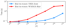
Figure 3: Response time of our proposed algorithm TED-Join, and WMMA-Ref an optimized MMA algorithm from Nvidia leveraging the WMMA API, using brute-force searches to compute Euclidean distance calculations on a 16-D exponentially distributed synthetic datasets.

IV-D Results: Optimized TC and CUDA Core Approaches

We investigate in this section the performance of TED-Join, as compared to other state-of-the-art algorithms from the literature: GDS-Join, Super-EGO, and FGF-Hilbert.

IV-D1 Uniformly Distributed Datasets

We start this result section with uniformly distributed synthetic datasets, detailed in Table I. We select this distribution as all the query points will have a similar number of candidate points to refine, allowing us to evaluate the performance of TCs when their workload is relatively uniform.

We show in Figure 4 the execution time of TED-Join compared to GDS-Join, Super-EGO, and FGF-Hilbert on a selection of uniformly distributed synthetic datasets. In these cases, we can see that Super-EGO is consistently performing worse than all of the other algorithms, except on the Unif8D10M dataset when $\epsilon=0.08$ (Figure 4(d)). Furthermore, we observe that TED-Join performs similarly or better than GDS-Join in most cases, except on Unif8D10M when $\epsilon<0.32$. From these results, it seems that TED-Join performs similar to GDS-Join when $\epsilon$ is low, and therefore when the workload is low as well, potentially indicating an overhead from using TCs. But when $\epsilon$ increases, and thus the workload, the higher computational throughput of TCs outperforms the CUDA cores used by GDS-Join.

We also observe that the speedup is the highest on the 2-D and 4-D datasets since all 2 or 4 dimensions can be computed at once using TCs, as we compute 4 dimensions at a time. The speedup is the lowest on the 6-D datasets since we need to compute the distances in two iterations (as many as for the 8-D datasets), but where 2 dimensions are zeros and thus that the CUDA cores in GDS-Join do not have to compute.

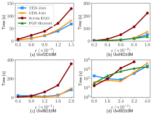
Figure 4: Response times of the TED-Join, GDS-Join, Super-EGO, and FGF-Hilbert on a selection of uniformly distributed synthetic datasets. $s$ is in the range (a) $282$–$6978$, (b) $71$–$8449$, (c) $7$–$4295$ and (d) $0$–$10888$. The legend in (a) corresponds to all subfigures. $d\in\{2,4,6,8\}$, $n=10$M.

IV-D2 Exponentially Distributed Datasets

In this section we present the results on the same algorithms as in Section IV-D1 on the exponentially distributed synthetic datasets, detailed in Table I. We select this distribution as it creates a large workload variance between the query points, where some query points may have many candidate points to refine, and other query points very few, which allows us to evaluate the performance of the TCs when their workload varies.

Figure 5 reports the execution time of TED-Join compared to GDS-Join, Super-EGO, and FGF-Hilbert on a selection of exponentially distributed synthetic datasets. Note that FGF-Hilbert did not run correctly on the 2-D and 6-D datasets (Figures 5(a) and (c)). In these experiments, TED-Join typically performs similarly or better than GDS-Join, particularly as $\epsilon$ increases. Super-EGO is consistently outperformed by the other algorithms, while FGF-Hilbert performs the best on the Expo4D10M dataset (Figure 5(b)), but is outperformed by both TED-Join and GDS-Join on the Expo8D10M dataset (Figure 5(d)). Because these datasets are exponentially distributed, the workload throughout the computation of the similarity self-join can vary a lot. The query points in the denser regions of the dataset will have many candidate points to refine, and the query points in the sparse regions of the dataset may have only a few candidate points. Hence, and despite a highly varying workload, TED-Join remains more efficient in most cases compared to GDS-Join and all compared algorithms in general, particularly in lower dimensions ($2\leq d\leq 4$).

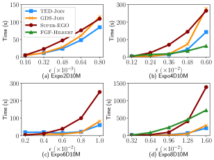
Figure 5: Response times of TED-Join, GDS-Join, Super-EGO, and FGF-Hilbert on a selection of exponentially distributed synthetic datasets. $s$ is in the range (a) $320$–$7834$, (b) $15$–$7414$, (c) $0$–$1658$ and (d) $0$–$1210$. The legend in (a) corresponds to all subfigures. $d\in\{2,4,6,8\}$, $n=10$M.

IV-D3 Real-World Datasets

We present in this section the results of TED-Join, GDS-Join, Super-EGO and FGF-Hilbert on a selection of the real-world datasets (Table II), as shown in Figure 6. TED-Join and GDS-Join perform very similarly, particularly on the higher dimensional datasets (Figures 6(b)–(d)), while TED-Join outperforms GDS-Join on the SW3DA dataset as $\epsilon$ increases (Figure 6(a)). FGF-Hilbert also performs quite similarly to TED-Join and GDS-Join, while Super-EGO is often outperformed by the other algorithms. Overall, these experiments show that TED-Join and GDS-Join may perform similarly as dimensionality increases, while TED-Join yields an advantage in lower dimensions (Figure 6(a)), as we observed in previous Figures 4 and 5. These experiments show us that in higher dimensions (Figures 6(b)–(d)), TED-Join may not yield an advantage compared to GDS-Join.

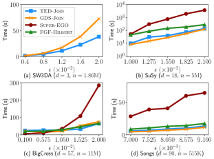
Figure 6: Response times of TED-Join, GDS-Join, Super-EGO, and FGF-Hilbert on a selection of real-world datasets (Table II). $s$ is in the range (a) $163$–$5373$, (b) $5$–$1090$, (c) $1$–$1104$ and (d) $127$–$998$. The legend in (a) corresponds to all subfigures.

IV-E Discussion: When Tensor Cores Should Be Employed

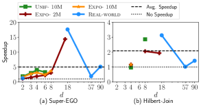
Figure 7: Speedups of TED-Join over (a) Super-EGO and (b) FGF-Hilbert across datasets presented in Tables I and II, for all values of $\epsilon$ we used, and as a function of the dimensionality. The dashed horizontal lines correspond to the average speedups of TED-Join over a compared algorithm, and the dotted horizontal lines represent no speedup.

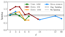
Figure 8: The same as for Figure 7, but plotting the speedup of TED-Join over GDS-Join.

We summarize the results of TED-Join as compared to the Super-EGO [9], FGF-Hilbert [8], and GDS-Join [6] algorithms that we obtained across experiments, including those that were omitted due to space constraints. The experiments covered a wide range of data dimensionalities, sizes, and distributions, resulting in an insightful picture of the overall performance of using TCs in TED-Join compared to the use of CUDA cores in GDS-Join. We report the speedup of TED-Join over the Super-EGO, FGF-Hilbert, and GDS-Join algorithms in Figures 7(a) and (b), and Figure 8, respectively. We also report the L1 and L2 cache hit rates of GDS-Join and TED-Join in Table III, and the average and maximum speedups of TED-Join over Super-EGO, FGF-Hilbert, and GDS-Join in Table IV.

Table III: L1 and L2 cache hit rates of GDS-Join and TED-Join on a selection of exponentially distributed synthetic datasets ($2\leq d\leq 16$, $n=2$M) and real-world datasets (SW3DA and SuSy), measured using the Nvidia Nsight Compute profiler.

	GDS-Join		TED-Join
Dataset	L1	L2	L1	L2
Expo2D2M	71.55%	97.85%	66.40%	98.11%
Expo4D2M	89.89%	95.60%	67.20%	97.65%
Expo8D2M	90.53%	97.15%	45.76%	66.23%
Expo16D2M	97.27%	99.84%	52.15%	57.27%
SW3DA	68.84%	97.62%	54.70%	94.43%
SuSy	92.13%	86.91%	38.00%	53.50%

Table IV: Average and maximum speedup of TED-Join over Super-EGO, FGF-Hilbert, and GDS-Join across experiments reported in Figures 7 and 8.

	CPU		GPU
	Super-EGO	FGF-Hilbert	GDS-Join ($d\leq 4$)
Average	$5.00\times$	$2.09\times$	$1.07\times$ ($1.28\times$)
Maximum	$27.22\times$	$9.46\times$	$2.23\times$ ($2.23\times$)

Figure 7(a) plots the speedup of TED-Join over the CPU algorithm Super-EGO [7, 9]. We observe that TED-Join consistently achieves a speedup $>1$, with an average of $5.00\times$ and a maximum of $27.22\times$. Thus, we believe that there is no clear disadvantage to using TED-Join over Super-EGO, regardless of the dimensionality, dataset distribution, or size.

Figure 7(b) plots the speedup of TED-Join over the CPU algorithm FGF-Hilbert [8]. Because many of our experiments could not be correctly conducted using the FGF-Hilbert algorithm, it makes it harder to draw a clear conclusion regarding the performance TED-Join compared to FGF-Hilbert. However, in the successful experiments, our TCs solution achieved an average speedup of $2.09\times$ with a maximum of $9.46\times$, and the majority of the speedups are above 1. Hence, and similarly to Super-EGO, there is no clear disadvantage of using TED-Join over FGF-Hilbert.

Observing the speedup of TED-Join over the CUDA core algorithm GDS-Join (Figure 8), we achieve the best performance when $d\leq 4$, and is best on exponentially distributed synthetic and real-world datasets. However, as the dimensionality $d$ increases, this speedup decreases, resulting in an average speedup of only $1.07\times$, but achieving a maximum of $2.23\times$ on the Expo3D2M dataset. If we only consider datasets where $d\leq 4$, TED-Join achieves an average speedup of $1.28\times$ over GDS-Join. Regarding the relatively low speedup in higher dimensions, TCs are designed for large matrix multiplications, where data can be reused when computing tiles of the resulting matrix. In the case of TED-Join, we are unable to reuse such data, thus limiting the performance. Additionally, we measure and compare the L1 and L2 cache hit rates of GDS-Join and TED-Join (Table III). While GDS-Join consistently achieves high cache hit rates, as the dimensionality increases, the cache hit rate using TED-Join decreases significantly. This explains why the speedup of TED-Join over GDS-Join decreases with increasing dimensionality (Figure 8).

From these results, we conclude that TCs should be used when the dimensionality is low ($2\leq d\leq 4$). Furthermore, there are cases where the dimensionality does not evenly divide by 4 (the dimension of the matrices as defined by the WMMA API for FP64). In total, $\lceil d/4\rceil$ MMA operations are needed to compute distance calculations, meaning that an additional MMA operation needs to be performed for cases where $d$ mod $4\neq 0$, which performs excess work. For example, because 6-D datasets are stored as 8-D datasets, where the last two dimensions are filled with zeros, TCs cannot achieve peak performance.

In summary, TCs should be used under the following scenarios instead of the reference implementations on their respective architectures:

•Compared to using CUDA cores, TCs should be used on low-dimensional datasets ($2\leq d\leq 4$).

•There is no drawback of using TCs over multi-core CPUs.

V Conclusion and Future Work

In this paper, we presented a novel approach to computing Euclidean distances leveraging TCs on Nvidia GPUs. TCs are designed solely for Matrix Multiply-Accumulate operations, and yield a much higher peak throughput than CUDA cores for this operation [2]. While TCs have been extensively used in fields such as machine learning, their usage remains very limited for more general-purpose applications. Hence, to our knowledge, this paper presents the first use of TCs for FP64 Euclidean distance calculations, where FP64 TCs computation has only been possible using the Ampere generation of Nvidia GPUs. This makes our algorithm suitable for scenarios where precise computation using FP64 is required. As such, our algorithm can provide the foundation for improving the performance of other data analysis applications where distance calculations are used (e.g., distance similarity searches, $k$NN, and DBSCAN [6, 7, 8, 9, 10, 11]). In these cases, our TC GPU kernel can be adapted to refine candidate points independently of the index that is used.

Comparison to tensor algorithms: we compared TED-Join to a reference MMA implementation, WMMA-Ref, from Nvidia [27], where no optimizations (including an index) were used. We find that TED-Join outperforms WMMA-Ref, because the latter requires unified memory to store a $|V|\times|V|$ distance matrix. Libraries such as cuBLAS and CUTLASS have the same drawbacks as WMMA-Ref, and are thus also unsuitable for moderately sized input datasets.

Comparison to similarity search reference implementations: we compared TED-Join to the GPU algorithm GDS-Join [6]. Despite an average speedup of $1.07\times$ over GDS-Join when $2\leq d\leq 90$, we achieve a maximum speedup of $2.23\times$ over this algorithm. We find that TED-Join yields the best performance when $d\leq 4$ with an average speedup of $1.28\times$ over GDS-Join. Because TED-Join and GDS-Join use the same index, this performance improvement is a direct result of employing TCs. While the maximum speedup is expected to be $2\times$ due to the maximum throughput of TCs compared to CUDA cores [2], we achieve a lower speedup on average because we rely on operations using CUDA cores. As described in Section III-A, combining CUDA and TCs to compute FP64 Euclidean distances is required due to the restricted matrix sizes when using the WMMA API and FP64.

Compared to the multi-core CPU algorithms Super-EGO [7] and FGF-Hilbert [8], we find that TED-Join typically outperforms these algorithms.

Future work includes, investigating cache and shared memory efficiency, particularly for higher dimensions, modeling TC performance to determine in which scenarios they should be leveraged instead of CUDA cores, using other floating point precisions available for TCs, and incorporating our TC GPU kernel into other algorithms, such as $k$NN [10], and particle simulations such as those in molecular dynamics [30].

References

- [1] Nvidia, “Nvidia Turing Architecture Whitepaper,” 2018, accessed: Nov. 14th, 2022. [Online]. Available: https://images.nvidia.com/aem-dam/en-zz/Solutions/design-visualization/technologies/turing-architecture/NVIDIA-Turing-Architecture-Whitepaper.pdf
- [2] ——, “Nvidia A100 Architecture Whitepaper,” 2020, accessed: Nov. 14th, 2022. [Online]. Available: https://www.nvidia.com/content/dam/en-zz/Solutions/Data-Center/nvidia-ampere-architecture-whitepaper.pdf
- [3] ——, “Nvidia H100 Architecture Whitepaper,” 2022, accessed: Nov. 14th, 2022. [Online]. Available: https://www.nvidia.com/hopper-architecture-whitepaper
- [4] Nvidia, “CUDA C++ Programming Guide,” 2022, accessed: Nov. 14th, 2022. [Online]. Available: https://docs.nvidia.com/cuda/cuda-c-programming-guide
- [5] J. Appleyard and S. Yokim, “Programming Tensor Cores in CUDA 9,” 2017, accessed: Nov. 14th, 2022. [Online]. Available: "https://developer.nvidia.com/blog/programming-tensor-cores-cuda-9/"
- [6] M. Gowanlock and B. Karsin, “GPU-Accelerated Similarity Self-Join for Multi-Dimensional Data,” Proc. of the 15th Intl. Workshop on Data Management on New Hardware, 2019, https://bitbucket.org/mikegowanlock/gpu_self_join/, Accessed: Nov. 14th, 2022.
- [7] D. V. Kalashnikov, “Super-EGO: Fast Multi-Dimensional Similarity Join,” The VLDB Journal, vol. 22, no. 4, pp. 561–585, 2013, accessed: Nov. 14th, 2022. [Online]. Available: https://www.ics.uci.edu/~dvk/code/SuperEGO.html
- [8] M. Perdacher, C. Plant, and C. Böhm, “Cache-Oblivious High-Performance Similarity Join,” Intl. Conf. on Management of Data, p. 87–104, 2019, https://gitlab.cs.univie.ac.at/martinp16cs/hilbertJoin, Accessed: Nov. 14th, 2022.
- [9] B. Gallet and M. Gowanlock, “Heterogeneous CPU-GPU Epsilon Grid Joins: Static and Dynamic Work Partitioning Strategies,” Data Science and Engineering, vol. 6, pp. 39–62, 2020.
- [10] M. Gowanlock, “Hybrid KNN-join: Parallel nearest neighbor searches exploiting CPU and GPU architectural features,” Journal of Parallel and Distributed Computing, vol. 149, pp. 119–137, 2021.
- [11] M. Ester, H.-P. Kriegel, J. Sander, and X. Xu, “A density-based algorithm for discovering clusters in large spatial databases with noise,” pp. 226–231, 1996.
- [12] E. Schubert, J. Sander, M. Ester, H. P. Kriegel, and X. Xu, “DBSCAN Revisited, Revisited: Why and How You Should (Still) Use DBSCAN,” ACM Trans. Database Syst., vol. 42, no. 3, jul 2017.
- [13] A. Dakkak, C. Li, J. Xiong, I. Gelado, and W.-m. Hwu, “Accelerating Reduction and Scan Using Tensor Core Units,” Proc. of the ACM Intl. Conf. on Supercomputing, p. 46–57, 2019.
- [14] Z. Ji and C.-L. Wang, “Accelerating DBSCAN Algorithm with AI Chips for Large Datasets,” 50th Intl. Conf. on Parallel Processing, 2021.
- [15] T. Ahle and F. Silvestri, “Similarity Search with Tensor Core Units,” Similarity Search and Applications, pp. 76–84, 2020.
- [16] B. Li, S. Cheng, and J. Lin, “tcFFT: A Fast Half-Precision FFT Library for NVIDIA Tensor Cores,” 2021 IEEE Intl. Conf. on Cluster Computing (CLUSTER), pp. 1–11, 2021.
- [17] T. Lu, Y.-F. Chen, B. Hechtman, T. Wang, and J. Anderson, “Large-Scale Discrete Fourier Transform on TPUs,” IEEE Access, vol. 9, pp. 93 422–93 432, 2021.
- [18] C. Böhm, R. Noll, C. Plant, and A. Zherdin, “Index-supported Similarity Join on Graphics Processors,” 2009, pp. 57–66.
- [19] C. Böhm, B. Braunmüller, F. Krebs, and H.-P. Kriegel, “Epsilon Grid Order: An Algorithm for the Similarity Join on Massive High-dimensional Data,” Proc. of the ACM SIGMOD Intl. Conf. on Management of Data, pp. 379–388, 2001.
- [20] M. Gowanlock, “Hybrid CPU/GPU Clustering in Shared Memory on the Billion Point Scale,” Proc. of the ACM Intl. Conf. on Supercomputing, p. 35–45, 2019.
- [21] “Space Weather datasets,” 2016. [Online]. Available: ftp://gemini.haystack.mit.edu/pub/informatics/dbscandat.zip
- [22] “OpenStreetMap Bulk GPS Point Data,” 2012, accessed: Nov. 14th, 2022. [Online]. Available: https://blog.openstreetmap.org/2012/04/01/bulk-gps-point-data/
- [23] “Gaia DR 2 Dataset,” 2018, accessed: Nov. 14th, 2022. [Online]. Available: https://cosmos.esa.int/web/gaia/dr2
- [24] P. Baldi, P. Sadowski, and D. Whiteson, “Searching for exotic particles in high-energy physics with deep learning,” Nature Communications, vol. 5, 2014.
- [25] M. R. Ackermann, M. Märtens, C. Raupach, K. Swierkot, C. Lammersen, and C. Sohler, “StreamKM++: A Clustering Algorithm for Data Streams,” ACM Journal of Experimental Algorithmics, vol. 17, May 2012.
- [26] T. Bertin-Mahieux, D. P. Ellis, B. Whitman, and P. Lamere, “The million song dataset,” Proc. of the 12th Intl. Conf. on Music Information Retrieval, 2011.
- [27] Nvidia, “Double Precision GEMM Using the WMMA API,” 2022, dmmaTensorCoreGemm.cu; Accessed: Nov. 14th, 2022. [Online]. Available: https://github.com/NVIDIA/cuda-samples
- [28] J. Schule, “Tensor Core Performance and Precision,” 2019, accessed: Nov. 14th, 2022. [Online]. Available: https://developer.nvidia.com/gtc/2019/video/s9176
- [29] V. Sarge and M. Andersch, “Tensor Core Performance on NVIDIA GPUs: The Ultimate Guide,” 2020, accessed: Nov. 14th, 2022. [Online]. Available: https://developer.nvidia.com/gtc/2020/video/s21929-vid
- [30] V. C. de Souza, L. Goliatt, and P. V. Z. Capriles Goliatt, “Clustering algorithms applied on analysis of protein molecular dynamics,” 2017 IEEE Latin American Conf. on Computational Intelligence (LA-CCI), pp. 1–6, 2017.