FusionVAE: A Deep Hierarchical Variational Autoencoder for RGB Image Fusion

Abstract

Sensor fusion can significantly improve the performance of many computer vision tasks. However, traditional fusion approaches are either not data-driven and cannot exploit prior knowledge nor find regularities in a given dataset or they are restricted to a single application. We overcome this shortcoming by presenting a novel deep hierarchical variational autoencoder called FusionVAE that can serve as a basis for many fusion tasks. Our approach is able to generate diverse image samples that are conditioned on multiple noisy, occluded, or only partially visible input images. We derive and optimize a variational lower bound for the conditional log-likelihood of FusionVAE. In order to assess the fusion capabilities of our model thoroughly, we created three novel datasets for image fusion based on popular computer vision datasets. In our experiments, we show that FusionVAE learns a representation of aggregated information that is relevant to fusion tasks. The results demonstrate that our approach outperforms traditional methods significantly. Furthermore, we present the advantages and disadvantages of different design choices.

1 Introduction

Sensor fusion is a popular technique in computer vision as it allows to combine the advantages from multiple information sources. It is especially gainful in scenarios where a single sensor is not able to capture all necessary data to perform a task satisfactorily. Over the last years, we have seen many examples, where the accuracy of computer vision tasks was significantly improved by sensor fusion, e.g. in environmental perception for autonomous driving [7, 30, 67], for 6D pose estimation [61, 17, 16], and for robotic grasping [72, 62]. However, traditional fusion methods usually focus more on the beneficial merging of multiple modalities and less on teaching the model to obtain profound prior knowledge about the used dataset.

Our work tries to fill in this research gap by proposing a deep hierarchical variational autoencoder called FusionVAE that is able to perform both tasks: fusing information from multiple sources and supplementing it with prior knowledge about the data gained while training. As shown in Fig. 1, FusionVAE merges a varying number of input images for reconstructing the original target image using prior knowledge about the dataset. To the best of our knowledge, FusionVAE is the first approach that combines these two tasks. Therefore, we developed three challenging benchmarks based on well-known computer vision datasets to evaluate the performance of our approach. In addition, we perform comparisons to baselines by extending traditional approaches to perform the same tasks. FusionVAE outperforms all these traditional methods on all proposed benchmark tasks significantly. We show that FusionVAE can generate high-quality images given few input images with partial observability. We provide ablation studies to illustrate the impact of commonly used information aggregation operations and to prove the benefits of the employed posterior distribution.

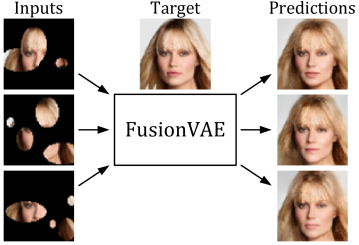
Figure 1: Overview of our FusionVAE approach. The network receives up to three partly occluded input images, fuses them together with prior knowledge, and predicts different hypothesis of how the target images could look like.

We can summarize the four main contributions of our paper as follows: i) We create three challenging image fusion tasks for generative models. ii) We develop a deep hierarchical VAE called FusionVAE that is able to perform image-based data fusion while employing prior knowledge of the used dataset. iii) We show that FusionVAE produces high-quality fused output images and outperforms traditional methods by a large margin. iv) We perform ablation studies showing the benefits of our design choices regarding both the posterior distribution and commonly used aggregation methods.

2 Related Work

In this section, we present related work about image generation, image fusion, and image completion.

2.1 VAE-based Image Generation

Variational autoencoders (VAE) are powerful networks that are able to compress the essence of datasets in a small latent space while being able to exploit it for generative tasks [27]. However, the standard VAE is limited in capacity and expressiveness and thus, when applied to image generation leads to over-smoothed results lacking fine-grained details. Over the last years much work has been invested into the effort of improving the generative performance of VAEs. One stream of work is based on introducing a hierarchy into the latent space of the VAE and scaling this hierarchy to greater and greater depth. First introduced in [54] many hierarchical VAEs are based on coupling the inference and generative processes by introducing a deterministic bottom-up path combined with a stochastic top-down process in the inference network and sharing the latter with the generative model. This setting has been extended by an additional deterministic top-down path and bidirectional inference in [44]. Recently, very deep hierarchical VAEs were realized in [8] by introducing residual bottlenecks with dedicated scaling, update skipping, and nearest neighbour up-sampling. Closest to our work is the recently proposed NVAE architecture [57], which relies on depth-wise convolution, residual posterior parametrization, and spectral regularization to enhance stability.

Other approaches propose increasing the expressiveness of VAEs by combining them with auto-regressive models like RNNs or PixelCNNs [6, 13, 50, 11], conditioning contexts (CVAE) [53, 60], normalizing flows [28], generative adversarial networks (GANs) [31, 46], or variational generative adversarial networks (CVAE-GAN) [1].

2.2 Fusion of Multiple Images

Image fusion has long been dominated by classical computer vision. Only lately deep learning methods entered the domain with the CNN-based approach proposed by Liu et al. [38]. In a subsequent publication the authors extended their work to a multi-scale setting [37]. Shortly afterwards, Prabhakar et al. developed a fusion method based on a siamese network architecture, called DeepFuse [48] which was improved in subsequent work [33] by employing the DenseNet architecture [20]. Concurrently, Li et al. [35] proposed a fusion architecture based on VGG [52] and in order to scale to even greater depth another one [34] based on ResNet-50 [15]. The aforementioned methods use CNNs as feature extractors and as decoders, while the fusion operations themselves are restricted to classical methods like averaging or addition of feature maps or weighted source images. A fully CNN-based feature-map fusion mechanism was proposed in [24].

While all previous publications target only a specific fusion task (e.g. multi-focus fusion, multi-resolution fusion, etc.) or were limited to specific domains (e.g. medical images), two very recent works propose novel multi-purpose fusion networks, which are applicable to many fusion tasks and image types [64, 71]. Very recently also GAN-based methods entered the domain of image fusion, starting with the work by Ma et al. on infrared-visible fusion [41, 43] and with [42, 63] on multi-resolution image fusion. Most recent are two publications on GAN-based multi-focus image fusion [14, 21]. While GAN-based approaches can generate high-fidelity images, it is known that they suffer from the mode collapse problem. VAE-based methods in contrast are known to generate more faithful data distribution [57]. Different from previous work, this paper proposes a VAE-based multi-purpose fusion framework.

2.3 Image Completion

Similar to image fusion, also image completion has only recently become a playing field for deep learning methods. First approaches based on simple multilayer perceptrons (MLPs) [29] or CNNs [12] were targeted only to filling small holes in an image. However, with the introduction of GANs [10], the area quickly became dominated by GAN-based approaches, starting with the context encoders presented by Pathak et al. [47]. Many subsequent papers proposed extensions to this model in order to obtain fine-grained completions while preserving global coherence by introducing additional discriminators [22], searching for closest samples to the corrupted image in a latent embedding space conditioning on semantic labels [56], or designing additional specialized loss functions [36]. High resolution results were obtained recently by multi-scale approaches [66], iterative upsampling [70], and the application of contextual attention [68, 55, 65]. Another stream of current work focuses on multi-hypothesis image completion, leveraging probabilistic problem formulations [73, 45].

3 Background

In this section, we outline the fundamentals of standard VAEs, conditional VAEs, and hierarchical VAEs upon which we build our approach. Another section is dedicated to aggregation methods for data fusion.

3.1 Standard VAE

A variational autoencoder (VAE) [27] is a neural network consisting of a probabilistic encoder $q(\boldsymbol{z}|\boldsymbol{y})$ and a generative model $p(\boldsymbol{y}|\boldsymbol{z})$. The generator models a distribution over the input data $\boldsymbol{y}$, conditioned on a latent variable $\boldsymbol{z}$ with prior distribution $p_{\theta}(\boldsymbol{z})$. The encoder approximates the posterior distribution $p(\boldsymbol{z}|\boldsymbol{y})$ of the latent variables $\boldsymbol{z}$ given input data $\boldsymbol{y}$ and is trained along with the generative model by maximizing the evidence lower bound (ELBO)

$${\rm ELBO}(\boldsymbol{y})=\mathbb{E}_{q(\boldsymbol{z}|\boldsymbol{y})}[\log p(\boldsymbol{y}|\boldsymbol{z})]-\text{KL}(q(\boldsymbol{z}|\boldsymbol{y})||p(\boldsymbol{z})),$$ (1)

where KL is the Kullback–Leibler divergence and $\log p(\boldsymbol{y})\geq{\rm ELBO}(\boldsymbol{y})$.

3.2 Conditional VAE

In VAEs, the generative model $p(\boldsymbol{y}|\boldsymbol{z})$ is unconditional. In contrast, conditional VAEs (CVAE) [53] consider a generative model for a conditional distribution $p(\boldsymbol{y}|\boldsymbol{x},\boldsymbol{z})$ where $\boldsymbol{y}$ is the target data, $\boldsymbol{x}$ is the conditional input variable, and $\boldsymbol{z}$ is a latent variable. The prior of the latent variable is $p(\boldsymbol{z}|\boldsymbol{x})$, while its approximate posterior distribution is given by $q(\boldsymbol{z}|\boldsymbol{x},\boldsymbol{y})$. The variational lower bound of the conditional log-likelihood can be written as follows

$$\log p(\boldsymbol{y}|\boldsymbol{x})\geq\mathbb{E}_{q(\boldsymbol{z}|\boldsymbol{x},\boldsymbol{y})}[\log p(\boldsymbol{y}|\boldsymbol{x},\boldsymbol{z})]-\text{KL}(q(\boldsymbol{z}|\boldsymbol{x},\boldsymbol{y})||p(\boldsymbol{z}|\boldsymbol{x})).$$ (2)

3.3 Hierarchical VAE

In hierarchical VAEs [54, 57, 25], the latent variables $\boldsymbol{z}$ are divided into $L$ disjoint groups $\boldsymbol{z}_{1},...,\boldsymbol{z}_{L}$ in order to increase the expressiveness of both prior and approximate posterior which become

$$p(\boldsymbol{z})=\prod_{l=1}^{L}p(\boldsymbol{z}_{l}|\boldsymbol{z}_{<l})\quad\text{and}\quad q(\boldsymbol{z}|\boldsymbol{y})=\prod_{l=1}^{L}q(\boldsymbol{z}_{l}|\boldsymbol{z}_{<l},\boldsymbol{y}),$$ (3)

where $\boldsymbol{z}_{<l}$ denotes the latent variables in all previous hierarchies. All the conditionals in the prior $p(\boldsymbol{z}_{l}|\boldsymbol{z}_{<l})$ and in the approximate posterior $q(\boldsymbol{z}_{l}|\boldsymbol{z}_{<l},\boldsymbol{y})$ are modeled by factorial Gaussian distributions. Under this modelling choice, the ELBO from Eq. 1 turns into

$${\rm ELBO}(\boldsymbol{y})=\mathbb{E}_{q(\boldsymbol{z}|\boldsymbol{y})}[\log p(\boldsymbol{y}|\boldsymbol{z})]-\sum_{l=1}^{L}\mathbb{E}_{q(\boldsymbol{z}_{<l}|\boldsymbol{y})}[\text{KL}(q(\boldsymbol{z}_{l}|\boldsymbol{z}_{<l},\boldsymbol{y})||p(\boldsymbol{z}_{l}|\boldsymbol{z}_{<l}))].$$ (4)

3.4 Aggregation Methods

For fusing data within our approach, we consider different aggregation methods, such as mean aggregation, max aggregation, Bayesian aggregation [59] and pixel-wise addition. All described aggregation methods fuse a set of feature tensors $\boldsymbol{f}_{1},...,\boldsymbol{f}_{K}$, obtained by encoding $K$ input images $\{\boldsymbol{x}_{i}\}_{i=1}^{K}$ in a permutation invariant way [69]. In mean aggregation, multiple feature vectors are fused by taking the pixel-wise average $\boldsymbol{f}=\frac{1}{K}\sum^{K}_{i=1}\boldsymbol{f}_{i}$. For max aggregation, we take the pixel-wise maximum instead $\boldsymbol{f}=\max_{i}(\boldsymbol{f}_{i})$. Bayesian aggregation (BA) [59] considers an uncertainty estimate for the fused feature vectors. In order to obtain such an uncertainty estimate, the encoder has to predict means $\boldsymbol{\mu}_{i}$ and variances $\boldsymbol{\sigma}_{i}$ of a factorized Gaussian distribution over the latent feature vectors

$$\boldsymbol{f}_{i}=\mathcal{N}(\boldsymbol{\mu}_{i},\text{diag}(\boldsymbol{\sigma}_{i})),\text{with~{}}\boldsymbol{\mu}_{i}=\text{enc}_{\mu}(\boldsymbol{x}_{i},\boldsymbol{y})\text{~{}and~{}}\boldsymbol{\sigma}_{i}=\text{enc}_{\sigma}(\boldsymbol{x}_{i},\boldsymbol{y}),$$ (5)

instead of $\boldsymbol{f}_{i}$ directly. Here $\text{enc}_{\mu}$ and $\text{enc}_{\sigma}$ represent the encoding process which generates means and variances respectively. The predicted distributions over latent feature vectors for multiple input images can be fused iteratively using the Bayes rule [2] (detailed derivation is given in Appendix 0.B)

$$\boldsymbol{q}_{i}=\boldsymbol{\sigma}^{2}_{i-1}\oslash(\boldsymbol{\sigma}^{2}_{i-1}+\boldsymbol{\sigma}^{2}_{i})$$ (6)

$$\text{where~{}}\boldsymbol{\mu}_{i}=\boldsymbol{\mu}_{i-1}+\boldsymbol{q}_{i}\odot(\boldsymbol{\mu}_{i}-\boldsymbol{\mu}_{i-1})\quad\text{and~{}}\quad\boldsymbol{\sigma}^{2}_{i}=\boldsymbol{\sigma}^{2}_{i-1}\odot(1-\boldsymbol{q}_{i}).$$ (7)

$\oslash$ and $\odot$ denote element-wise division and multiplication respectively.

4 Conditional Generative Models for Image Fusion

We propose a deep hierarchical conditional variational autoencoder, called FusionVAE (Fusion Variational Auto-Encoder), that is able to fuse information from multiple sources and to infer the missing information in the images from a prior learned from the dataset. To the best of our knowledge, it is the first model that combines the generative ability of a hierarchical VAE to learn the underlying distribution of complex datasets with the ability to fuse multiple input images.

4.1 Problem Formulation

We consider image fusion problems that are concerned with generating the fused target image from multiple source images. Each source image contains partial information of the target image and the goal of the task is to recover the original target image given a finite set of source images. In particular, we denote the target image as $\boldsymbol{y}$ and the set of $K$ source images as context $\boldsymbol{x}=\{\boldsymbol{x}_{1},\,\boldsymbol{x}_{2},\,\ldots,\,\boldsymbol{x}_{K}\}$, where each $\boldsymbol{x}_{i}$ is one source image. Given training sample $(\boldsymbol{x},\boldsymbol{y})$, we aim to maximize the conditional likelihood $p(\boldsymbol{y}|\boldsymbol{x})$.

4.2 FusionVAE

Our approach is designed to maximize the conditional likelihood $p(\boldsymbol{y}|\boldsymbol{x})$. However, optimizing this objective directly is intractable. Therefore, we derive a variational lower bound as follows (detailed derivation can be found in Appendix 0.C)

$$\begin{split}\log p(\boldsymbol{y}|\boldsymbol{x})&\geq\mathbb{E}_{q_{\phi}(\boldsymbol{z}|\boldsymbol{y})}[\log p_{\theta}(\boldsymbol{y}|\boldsymbol{x},\boldsymbol{z})]\\ &-\beta\sum_{l=1}^{L}\alpha_{l}\mathbb{E}_{q(\boldsymbol{z}_{<l}|\boldsymbol{y})}[\text{KL}(q_{\phi}(\boldsymbol{z}_{l}|\boldsymbol{y},\boldsymbol{z}_{<l})||p_{\theta}(\boldsymbol{z}_{l}|\boldsymbol{x},\boldsymbol{z}_{<l}))],\end{split}$$ (8)

where we split the latent variables $\boldsymbol{z}$ into $L$ disjoint groups $\{\boldsymbol{z}_{1},\,\boldsymbol{z}_{2},\,\ldots,\,\boldsymbol{z}_{L}\}$. $\beta$ and $\alpha_{l}$ are annealing parameters that control the warming-up of the KL terms as in [57]. Inspired by [54], $\beta$ is increased linearly from 0 to 1 during the first few training epochs to start training the reconstruction before introducing the KL term, which is increased gradually. $\alpha_{l}$ is a KL balancing coefficient [58] that is used during the warm-up period to encourage the equal use of all latent groups and to avoid posterior collapse.

FusionVAE consists of three main networks and a latent space as illustrated in Fig. 2: 1) a context encoder network which models the conditional prior $p_{\phi}(\boldsymbol{z}_{l}|\boldsymbol{x},\boldsymbol{z}_{<l})$, 2) a target encoder which models the approximate posterior $q_{\phi}(\boldsymbol{z}|\boldsymbol{y})$, 3) a latent space comprising the $L$ latent groups, and 4) a generator network $p_{\theta}(\boldsymbol{y}|\boldsymbol{x},\boldsymbol{z})$ that aims to reconstruct the target image.

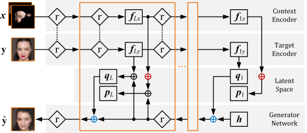
Figure 2: Overview of the proposed network architecture. $\boldsymbol{h}$ is a trainable parameter vector, $\boldsymbol{\oplus}$ denotes concatenation, $\boldsymbol{\oplus}$ max aggregation, and $\boldsymbol{\oplus}$ pixel-wise addition. is a residual network like in [57]. The dotted lines between the residual networks indicate shared parameters.

4.3 Network Architecture

Fig. 2 illustrates the network architecture of our FusionVAE for training. It is built in a hierarchical way inspired by [57]. In each latent hierarchy $l\in 1,\,\ldots,\,L$ we have a set of feature maps $\boldsymbol{f}_{lx}$, $\boldsymbol{f}_{ly}$ and latent distributions $p_{l}$, $q_{l}$.

The first gray box contains the context encoder network that obtains a stack of source images $\boldsymbol{x}$ and employs residual cells [15] as in [57] to extract features $\boldsymbol{f}_{lx}$. The second gray box shows the target encoder network that encodes the target image $\boldsymbol{y}$ into the feature map $\boldsymbol{f}_{ly}$ using the same residual cells as the context encoder. The third gray box illustrates the latent space which contains the prior distributions $p_{\phi}(\boldsymbol{z}_{l}|\boldsymbol{x},\boldsymbol{z}_{<l})$ (denoted $p_{1},\,...,\,p_{L}$ in Fig. 2) and the approximate posterior distributions $q_{\phi}(\boldsymbol{z}_{l}|\boldsymbol{y},\boldsymbol{z}_{<l})$ (denoted $q_{1},\,...,\,q_{L}$ in Fig. 2). The fourth gray box contains the generator network which aims to create different output samples $\boldsymbol{\hat{y}}$. It employs a trainable parameter vector $\boldsymbol{h}$, concatenates the information from all hierarchies, and decodes them using residual cells.

In each latent hierarchy, we aggregate the context features $\boldsymbol{f}_{lx}$ using pixel-wise max aggregation. In all but the first hierarchy, we pixel-wisely add the corresponding feature map from the generator network to the aggregated context features and to the target image features $f_{ly}$. Using 2D convolutional layers, we learn the prior distributions $p_{l}$ and the approximate posterior distributions $q_{l}$. We propose to use the approximate posterior distributions $q_{l}$ as target distributions in order to learn good prior distributions $p_{l}$. Therefore, $q_{\phi}(\boldsymbol{z}_{l}|\boldsymbol{y},\boldsymbol{z}_{<l})$ is created from the target image features $f_{ly}$ as well as information from the generator network.

During training the generator network aims to create a prediction $\boldsymbol{\hat{y}}$ based on samples of the posterior distributions $q_{l}$ and a trainable parameter vector $\boldsymbol{h}$.

For evaluation, we can omit the target image input $\boldsymbol{y}$ and sample from the prior distributions $p_{l}$. In case no input image is given, we set $p_{1}$ to a standard normal distribution. Based on the samples and the trainable parameter vector $\boldsymbol{h}$, our FusionVAE can generate new output images.

5 Experimental Setup

To evaluate our approach, we conduct a series of experiments on three different datasets using data augmentation. Furthermore, we adapt traditional architectures for solving the same tasks in order to compare our results. Finally, we perform an ablation study to show the effects of specific design choices.

5.1 Datasets

For training and evaluating our approach, we create three novel fusion datasets based on MNIST [32], CelebA [39], and T-LESS [18] as described in the following.

FusionMNIST.

Based on the dataset MNIST [32], we create an image fusion dataset called FusionMNIST. For each target image, it contains different noisy representations where only random parts of the target image are visible. The first three columns of Fig. 3 show different examples of FusionMNIST corresponding to the target images in the fourth column. To generate FusionMNIST, we applied zero padding to all MNIST images to obtain a resolution of $32\times 32$. For creating a noisy representation, we generate a mask composed of the union of a varying number of ellipses with random size, shape and position. All parts of the given images outside the mask are blackened. Finally, we add Gaussian noise with a fixed variance and clip the pixel values afterwards to stay within $[0,1]$.

FusionCelebA.

We generate a similar fusion dataset based on the aligned and cropped version of CelebA [39] which we call FusionCelebA. Fig. 4 depicts different example images in the first three columns which belong to the target image in the fourth column. To generate FusionCelebA, we center-crop the CelebA images to $148\times 148$ before scaling them down to $64\times 64$ as proposed by [31]. As in FusionMNIST, we create different representations by using masks based on random ellipses.

FusionT-LESS.

A promising area of application for our FusionVAE is robot vision. Scenes in robotics settings can be very difficult to understand due to texture-less or reflective objects and occlusions. To examine the performance of our FusionVAE in this area, we create an object dataset with challenging occlusions based on T-LESS [18] which we call FusionT-LESS. To generate FusionT-LESS, we use the real training images of T-LESS and take all images of classes 19 – 24 as basis for the target images. This selection contains all objects with power sockets and therefore images with many similarities. Every tenth image is removed from the training set and used for evaluation. In order to create challenging occlusions, we cut all objects from images of other classes using a Canny edge detector [5] and overlay each target image with a random number between five and eight cropped objects. We select all images from classes 1, 2, 5 – 7, 11 – 14, and 25 – 27 as occluding objects for training and classes 3, 4, 8 – 10, 15 – 18, and 28 – 30 for evaluation.

5.2 Data Augmentation

During training we apply different augmentation methods on the datasets to avoid overfitting. For FusionMNIST, we apply the elliptical mask generation and the addition of Gaussian noise live during training so that we obtain an infinite number of different fusion tasks. For FusionT-LESS, almost the entire creation of occluded images is performed during training. We apply horizontal flips, rotations, scaling and movement of target and occluding images with random parameters before composing the different occluded representations. Solely the object cutting with the Canny edge detector is performed offline as a pre-processing step to keep the training time low. For FusionCelebA, we apply a horizontal flip of all images randomly in 50% of all occasions and also the elliptical mask generation is done live during training.

5.3 Architectures for Comparison

To the best of our knowledge, FusionVAE is the first fusion network for multiple images with a generative ability to fill areas without input information based on prior knowledge about the dataset under consideration. For lack of a suitable other model from the literature which would allow a fair comparison on our multi-image fusion tasks, we compare our approach with standard architectures that we adapted to support our tasks.

The first architecture for comparison is a CVAE with residual layers as employed in [57]. We use a shared encoder for processing the input images and applied max aggregation before the latent space as we did in our FusionVAE. The second architecture for comparison is a fully convolutional network (FCN) with shared encoder and max aggregation before the decoder.

For both baseline architectures, we created a version with skip connections (+S) and a version without. When using skip connections, we applied max aggregation at each shortcut for merging the features from the encoder with the decoder’s features. To allow for a fair comparison, we designed all architectures so that they have a similar number of trainable parameters.

5.4 Training Procedure

We trained all networks in a supervised manner using the augmented target images $\boldsymbol{y}$ as described in Sec. 5.2. In order to teach the networks both to fuse information from a different number of input images and to learn prior knowledge about the dataset, we vary the number of input images $\boldsymbol{x}$ during the entire training. Specifically, we select a uniformly distributed random number between zero and three for each batch.

5.5 Evaluation Metrics

For evaluation, we estimate the negative log-likelihood (NLL) in bits per dimension (BPD) using weighted importance sampling [4]. We use 100 samples for all experiments with FusionCelebA as well as FusionT-LESS and 1000 samples for FusionMNIST. Since we cannot estimate the NLL of the FCN, we used the minimum over all samples of the mean squared error ($\text{MSE}_{\min}$) as second metric.

6 Results

This section presents and discusses the quantitative and qualitative results of our research in comparison to the baseline methods mentioned in Sec. 5.3.

6.1 Quantitative Results

Tabs. 1, 2 and 3 show the NLL and the $\text{MSE}_{\min}$ of all architectures on FusionMNIST, FusionCelebA, and FusionT-LESS respectively. The results are divided into the results based on zero to three input images and the average (avg) of it. We see that our FusionVAE outperforms all baseline methods on average. Regarding the NLL, our model surpasses the others additionally for 0 and 1 input images. For 2 and 3 images, CVAE+S reaches sometimes slightly better NLL values. However, our approach reaches the best $\text{MSE}_{\min}$ values for each number of input images.

	NLL in $10^{-2}$ BPD					$\text{MSE}_{\min}$ in $10^{-2}$
	0	1	2	3	avg	0	1	2	3	avg
FCN						10.99	5.81	5.78	5.79	7.25
FCN+S						5.80	3.74	2.54	1.78	3.56
CVAE	17.81	15.01	14.07	13.61	15.23	3.83	1.72	1.05	0.80	1.93
CVAE+S	18.43	14.57	13.18	12.30	14.77	3.62	1.75	1.19	0.97	1.95
FusionVAE	15.93	14.17	13.70	13.48	14.39	3.14	0.99	0.74	0.65	1.45

Table 1: Results on FusionMNIST. The best results are printed in bold.

	NLL in $10^{-2}$ BPD					$\text{MSE}_{\min}$ in $10^{-2}$
	0	1	2	3	avg	0	1	2	3	avg
FCN						13.77	14.82	13.10	11.24	13.23
FCN+S						12.56	8.96	6.06	4.09	7.92
CVAE	446.0	280.1	273.5	266.5	316.7	9.23	3.46	2.27	1.55	4.14
CVAE+S	525.0	270.1	233.5	203.5	308.3	11.08	5.49	3.66	2.57	5.71
FusionVAE	248.1	227.6	231.2	228.7	233.9	5.11	0.88	0.86	0.84	1.93

Table 2: Results on FusionCelebA. The best results are printed in bold.

	NLL in $10^{-2}$ BPD					$\text{MSE}_{\min}$ in $10^{-2}$
	0	1	2	3	avg	0	1	2	3	avg
FCN						5.83	3.34	2.37	1.82	3.35
FCN+S						8.06	1.84	1.13	0.74	2.97
CVAE	25.24	23.73	22.70	23.13	23.71	5.57	1.54	0.77	0.37	2.08
CVAE+S	26.08	24.94	23.98	23.95	24.75	4.95	2.50	1.77	1.19	2.62
FusionVAE	24.18	23.07	22.23	22.88	23.10	4.11	0.59	0.32	0.19	1.32

Table 3: Results on FusionT-LESS. The best results are printed in bold.

6.2 Qualitative Results

The outstanding performance of our architecture in comparison to the others is also obvious when looking at the qualitative results in Figs. 3, 4 and 5. For every row, these figures show the input, target, and up to three output predictions for all architectures. For the FCN, we depict just a single output prediction per row as all of them look almost identical.

In the first three rows when the network does not receive any input image, we see that our network provides very realistic images. This indicates that it is able to capture the underlying distribution of the used datasets very well and much better than the other architectures. Due to the difficulty of the FusionT-LESS dataset, none of the models is able to produce realistic images without any input. Still our model shows much better performance in generating object-like shapes. In case the models receive at least one input image (cf. rows 4 – 12), all architectures are able to extract the available information from the given input images. In addition, all VAE approaches, ours included, are able to complete the given input data based on prior knowledge. It is clearly visible, however, that the predictions of our model are much more realistic than the ones of the standard CVAE approaches especially for the more difficult datasets like FusionCelebA and FusionT-LESS.

Figure 3: Prediction results of the different architectures on FusionMNIST for zero to three input images.

Figure 4: Predictions on FusionCelebA for zero to three input images.

Figure 5: Predictions on FusionT-LESS for zero to three input images.

6.3 Ablation Studies

We conducted ablation studies to show the effect of certain design choices, such as the selection of the approximate posterior and the aggregation method. All experiments are run on the FusionCelebA dataset.

Tab. 4 compares the performance of our FusionVAE for two different approximate posterior distributions $q$. The approximate posterior we selected for our FusionVAE $q(y)$, depends only on the given target image $y$. It performs slightly better on average compared to the same method using a posterior that is computed based on the input images $x$ as well as the target image $y$. However, the latter approach is superior when fusing two or three input images.

	NLL in $10^{-2}$ BPD					$\text{MSE}_{\min}$ in $10^{-2}$
	0	1	2	3	avg	0	1	2	3	avg
$q(x,y)$	309.2	246.8	211.1	180.5	237.0	5.04	1.50	0.95	0.66	2.04
$q(y)$	248.1	227.6	231.2	228.7	233.9	5.11	0.88	0.86	0.84	1.93

Table 4: Posterior ablation on the FusionCelebA dataset. The best results are printed in bold.

	NLL in $10^{-2}$ BPD					$\text{MSE}_{\min}$ in $10^{-2}$
	0	1	2	3	avg	0	1	2	3	avg
MaxAggAdd	248.1	227.6	231.2	228.7	233.9	5.11	0.88	0.86	0.84	1.93
MeanAggAdd	270.9	223.3	216.4	214.4	231.3	5.41	1.00	0.79	0.70	1.98
BayAggAdd	970.7	294.0	291.4	291.5	462.6	6.03	5.17	5.10	5.12	5.36
MaxAggAll	249.6	236.0	223.9	212.7	230.6	6.15	2.82	1.84	1.30	3.03
MeanAggAll	252.7	235.2	222.2	213.5	230.9	6.19	2.39	1.52	1.13	2.81
BayAggAll	255.6	568.3	414.7	1376.9	653.3	5.10	4.24	1.96	1.39	3.18

Table 5: Aggregation ablation on the FusionCelebA dataset. The best results are printed in bold.

Tab. 5 shows the performance of different aggregation methods which are applied to create the prior distributions $p_{l}$ of every latent group. In our FusionVAE, the prior is created by fusing the input image features $f_{lx}$ using max aggregation (MaxAgg) and adding them to the decoded features of the same latent group before applying a 2D convolution. We abbreviate that method with MaxAggAdd.

In addition to MaxAgg, we examined mean aggregation (MeanAgg) and Bayesian aggregation (BayAgg) [59] for comparison. For each aggregation principle, we tried two different versions: 1) aggregation of the input image features $\boldsymbol{f}_{lx}$ adding the corresponding information from the decoder in a pixel-wise manner (denoted by suffix Add), and 2) directly aggregating all features, i.e. both input image features $\boldsymbol{f}_{lx}$ and decoder features (denoted by suffix All).

For creating the prior $p_{i}$ when using BayAgg, we moved the 2D convolutions before the aggregation in order to create the parameters $\mu$ and $\sigma$ of a latent Gaussian distribution. Unlike MaxAgg and MeanAgg, BayAgg directly outputs a new Gaussian distribution that does not need to be processed any further by a convolution.

We can see that all variations of mean and max aggregation are significantly better than Bayesian aggregation. Also their training procedures are less often impaired due to numeric instabilities. Interestingly, the NLL is very similar independent of whether the aggregation is performed on all features or not. However, the $\text{MSE}_{\min}$ is much better for the aggregation with addition. Since the expressiveness of the metrics is limited, we provide additional visualizations of this ablation in Appendix 0.D.

7 Conclusion

We have presented a novel deep hierarchical variational autoencoder for generative image fusion called FusionVAE. Our approach fuses multiple corrupted input images together with prior knowledge obtained during training. We created three challenging image fusion benchmarks based on common computer vision datasets. Moreover, we implemented four standard methods that we modified to support our tasks. We showed that our FusionVAE outperforms all other methods significantly while having a similar number of trainable parameters. The predicted images of our approach look very realistic and incorporate given input information almost perfectly. During ablation studies, we revealed the benefits of our design choices regarding the applied aggregation method and the used posterior distribution. In future work, our research could be extended by enabling the fusion of different modalities e.g. by using multiple encoders. Additionally, an explicit uncertainty estimation could be implemented that helps to weigh the impact of input information according to its uncertainty.

Supplementary Material

Appendix 0.A Implementation details

For FusionMNIST and FusionT-LESS, we model the decoder’s output by pixel-wise independent Bernoulli distributions. For FusionCelebA, we use pixel-wise independent discretized logistic mixture distributions as proposed by Salimans et al. [51].

The residual cells of the encoder are composed of batch normalization layers [23], Swish activation functions [49], convolutional layers, and Squeeze-and-Excitation (SE) blocks [19] as proposed in [57]. In the decoder, we also follow [57] and build the residual cells out of batch normalization layers, 1x1 convolutions, Swish activations, depthwise separable convolutions [9], and SE blocks. However, we omitted normalizing flow because in our experiments it showed to increase the training time without improving the prediction accuracy significantly.

For each dataset, we chose the size of the architecture individually to achieve acceptable accuracy while keeping the training time reasonable. Tab. 6 provides details about the used hyperparameters.

Hyperparameter	FusionMNIST	FusionCelebA	FusionT-LESS
# latent groups per scale	5, 2	10, 5, 2	10, 5, 2
spatial dimensions of $\boldsymbol{z}_{l}$ per scale	$4^{2},8^{2}$	$8^{2},16^{2},32^{2}$	$8^{2},16^{2},32^{2}$
# channels in $\boldsymbol{z}_{l}$	10	20	20
# GPUs	2	4	2
# training epochs	400	90	500
batch size	800	32	32
Training time	4h	48h	28h

Table 6: Main hyperparameters of our experiments.

In general, the number of latent groups $L$ should be chosen depending on the complexity of the task at hand. We made our decision based on the $L$ of the NVAE [57] but reduced it for computational reasons. For FusionCelebA and FusionT-LESS, we use 17 latent groups, for FusionMNIST only seven. Using more latent groups improves the results but increases the computational effort significantly.

For all experiments, we used GPUs of type NVIDIA Tesla V100 with 32GB of memory and trained with an AdaMax optimizer [26]. We applied a cosine annealing schedule for the learning rate [40] starting at 0.01 and ending at 0.0001.

Appendix 0.B Derivation of Bayesian Aggregation

We use two related encoders to learn a latent observation $\boldsymbol{\mu}_{i}=\text{enc}_{\mu}(\boldsymbol{x}_{i},\boldsymbol{y})$ with its corresponding variance values $\boldsymbol{\sigma}_{i}=\text{enc}_{\sigma}(\boldsymbol{x}_{i},\boldsymbol{y})$.

Assuming a factorized Gaussian prior distribution in the latent space $p(\boldsymbol{z})=\mathcal{N}(\boldsymbol{z}|\boldsymbol{\mu}_{\boldsymbol{z},0},\text{diag}(\boldsymbol{\sigma}_{\boldsymbol{z},0}))$, we can derive the factorized posterior distribution $q_{\phi}(\boldsymbol{z}|\boldsymbol{y})=\mathcal{N}(\boldsymbol{z}|\boldsymbol{\mu}_{z},\text{diag}(\boldsymbol{\sigma}_{z})$ in closed form using standard Gaussian conditioning [3] following [59]

$$\boldsymbol{\sigma}_{\boldsymbol{z}}^{2}=\left[(\boldsymbol{\sigma}_{\boldsymbol{z},0}^{2})^{\ominus}+(\boldsymbol{\sigma}_{i}^{2})^{\ominus}\right]^{\ominus},$$ (9)

$$\boldsymbol{\mu}_{\boldsymbol{z}}=\boldsymbol{\mu}_{\boldsymbol{z},0}+\boldsymbol{\sigma}_{\boldsymbol{z},0}^{2}\odot(\boldsymbol{\mu}_{i}-\boldsymbol{\mu}_{\boldsymbol{z},0})\oslash\boldsymbol{\sigma}_{i}^{2}$$ (10)

where $\ominus$ denotes element-wise inversion, $\odot$ denotes element-wise multiplication, and $\oslash$ denotes element-wise division.

Appendix 0.C Derivation of FusionVAE’s ELBO

We start with the following KL divergence between the approximate posterior and the real posterior,

$$\mathrm{KL}(q_{\theta}(\boldsymbol{z}|\boldsymbol{y})||p_{\theta}(\boldsymbol{z}|\boldsymbol{x},\boldsymbol{y}))\geq 0.$$ (11)

Next, we apply the Bayes’s theorem to obtain

$$-\int q_{\theta}(\boldsymbol{z}|\boldsymbol{y})\log\frac{p(\boldsymbol{y}|\boldsymbol{x},\boldsymbol{z})p(\boldsymbol{z}|\boldsymbol{x})}{p(\boldsymbol{y}|\boldsymbol{x})q_{\theta}(\boldsymbol{z}|\boldsymbol{y})}dz\geq 0.$$ (12)

This leads to

$$\begin{split}-\mathbb{E}_{q_{\theta}(\boldsymbol{z}|\boldsymbol{y})}[\log p(\boldsymbol{y}|\boldsymbol{x},\boldsymbol{z})]&-\mathrm{KL}(q_{\theta}(\boldsymbol{z}|\boldsymbol{y})||p(\boldsymbol{z}|\boldsymbol{x}))\\ &+\int q_{\theta}(\boldsymbol{z}|\boldsymbol{y})\log p(\boldsymbol{y}|\boldsymbol{x})dz\geq 0.\end{split}$$ (13)

The term $\log p(\boldsymbol{y}|\boldsymbol{x})$ can be moved out from the third integral component, and leaves the integral becoming 1. Finally, we obtain the ELBO of the conditional log-likelihood

$$\log p(\boldsymbol{y}|\boldsymbol{x})\geq\mathbb{E}_{q_{\theta}(\boldsymbol{z}|\boldsymbol{y})}[\log p(\boldsymbol{y}|\boldsymbol{x},\boldsymbol{z})]+\mathrm{KL}(q_{\theta}(\boldsymbol{z}|\boldsymbol{y})||p(\boldsymbol{z}|\boldsymbol{x})).$$ (14)

Appendix 0.D Ablation Studies

This is a supplement for the aggregation ablation study in Sec. 6.3. In Tab. 5, we saw that the average NLL of all experiments using mean and max aggregation methods are similar. Fig. 6 shows the corresponding qualitative results. However, even though the NLL is very similar, the results of the aggregation of all features (MaxAggAll and MeanAggAll) are much more blurry than the results of the aggregation with addition (MaxAggAdd and MeanAggAdd). This is in conformity with the $\text{MSE}_{\min}$ results. It indicates that the NLL alone is not always the best metric to assess the visual closeness to real faces. When carefully examining the images of the addition aggregations, you could argue that the predictions with zero input images look slightly more realistic for max aggregation while for three input images, mean aggregation seems to be marginally better. This again confirms the validity of the $\text{MSE}_{\min}$ results even though the NLL results are also in accordance for this comparison.

Figure 6: Prediction results of the different aggregation methods on FusionCelebA for zero to three input images.

Appendix 0.E Statistic Significance of the Results

All experiments for this publications were carefully designed and optimized so that the training procedures are stable and lead to reproducible results. However, the data processing pipelines introduce randomness which lead to non-deterministic training outcomes due to multi-GPU training. We therefore ran every experiment three times and reported the results of the best training in Sec. 6. In Tabs. 7, 8, 9, 10, 11 and 12 we provide the means and variances of the three training runs.

	0	1	2	3	avg
CVAE	$17.67\pm 0.10$	$15.11\pm 0.07$	$14.19\pm 0.08$	$13.71\pm 0.07$	$15.27\pm 0.02$
CVAE+S	$18.45\pm 0.02$	$14.64\pm 0.06$	$\textbf{13.22}\pm 0.03$	$\textbf{12.32}\pm 0.02$	$14.81\pm 0.03$
FusionVAE	$\textbf{15.91}\pm 0.03$	$\textbf{14.13}\pm 0.07$	$13.64\pm 0.09$	$13.41\pm 0.10$	$\textbf{14.34}\pm 0.07$

Table 7: Mean and standard deviation of the FusionMNIST NLL results in $10^{-2}$ BPD. The best results are printed in bold.

	0	1	2	3	avg
FCN	$10.84\pm 0.37$	$5.96\pm 0.11$	$6.02\pm 0.18$	$6.13\pm 0.25$	$7.38\pm 0.11$
FCN+S	$6.21\pm 0.65$	$3.79\pm 0.04$	$2.64\pm 0.07$	$1.88\pm 0.08$	$3.73\pm 0.22$
CVAE	$3.87\pm 0.03$	$1.76\pm 0.03$	$1.09\pm 0.03$	$0.83\pm 0.02$	$1.97\pm 0.03$
CVAE+S	$3.53\pm 0.06$	$1.77\pm 0.01$	$1.23\pm 0.04$	$1.02\pm 0.04$	$1.96\pm 0.01$
FusionVAE	$\textbf{3.14}\pm 0.01$	$\textbf{1.04}\pm 0.06$	$\textbf{0.77}\pm 0.04$	$\textbf{0.67}\pm 0.03$	$\textbf{1.47}\pm 0.03$

Table 8: Mean and standard deviation of the FusionMNIST $\text{MSE}_{\min}$ results in $10^{-2}$. The best results are printed in bold.

	0	1	2	3	avg
CVAE	$456.9\pm~{}9.42$	$289.1\pm~{}6.53$	$278.9\pm~{}4.51$	$270.3\pm~{}3.66$	$324.0\pm~{}5.17$
CVAE+S	$487.4\pm 27.45$	$355.4\pm 60.39$	$280.7\pm 35.12$	$230.9\pm 22.59$	$338.8\pm 22.99$
FusionVAE	$\textbf{251.0}\pm~{}2.06$	$\textbf{222.3}\pm~{}3.71$	$\textbf{226.8}\pm~{}3.16$	$\textbf{224.0}\pm~{}3.36$	$\textbf{231.0}\pm~{}2.05$

Table 9: Mean and standard deviation of the FusionCelebA NLL results in $10^{-2}$ BPD. The best results are printed in bold.

	0	1	2	3	avg
FCN	$13.07\pm 0.87$	$20.00\pm 3.77$	$17.87\pm 3.42$	$15.56\pm 3.08$	$16.62\pm 2.48$
FCN+S	$11.94\pm 0.52$	$18.58\pm 7.02$	$14.90\pm 6.59$	$11.19\pm 5.39$	$14.15\pm 4.65$
CVAE	$8.70\pm 0.42$	$6.25\pm 2.16$	$4.33\pm 1.77$	$3.02\pm 1.37$	$5.58\pm 1.21$
CVAE+S	$9.87\pm 1.10$	$9.60\pm 3.34$	$7.30\pm 3.07$	$5.57\pm 2.64$	$8.09\pm 2.19$
FusionVAE	$\textbf{ 5.82}\pm 0.52$	$\textbf{ 1.10}\pm 0.16$	$\textbf{ 0.93}\pm 0.06$	$\textbf{ 0.84}\pm 0.03$	$\textbf{ 2.18}\pm 0.17$

Table 10: Mean and standard deviation of the FusionCelebA $\text{MSE}_{\min}$ results in $10^{-2}$. The best results are printed in bold.

	0	1	2	3	avg
CVAE	$25.27\pm 0.04$	$24.00\pm 0.25$	$22.98\pm 0.24$	$23.34\pm 0.19$	$23.90\pm 0.17$
CVAE+S	$26.12\pm 0.23$	$25.29\pm 0.27$	$24.27\pm 0.25$	$24.15\pm 0.20$	$24.97\pm 0.16$
FusionVAE	$\textbf{24.32}\pm 0.10$	$\textbf{23.09}\pm 0.02$	$\textbf{22.25}\pm 0.02$	$\textbf{22.90}\pm 0.02$	$\textbf{23.15}\pm 0.04$

Table 11: Mean and standard deviation of the FusionT-LESS NLL results in $10^{-2}$ BPD. The best results are printed in bold.

	0	1	2	3	avg
FCN	$5.88\pm 0.04$	$3.32\pm 0.10$	$2.50\pm 0.09$	$1.96\pm 0.10$	$3.43\pm 0.06$
FCN+S	$8.83\pm 1.05$	$1.95\pm 0.14$	$1.28\pm 0.15$	$0.86\pm 0.14$	$3.26\pm 0.37$
CVAE	$5.49\pm 0.11$	$1.73\pm 0.22$	$0.95\pm 0.18$	$0.44\pm 0.07$	$2.18\pm 0.13$
CVAE+S	$4.87\pm 0.06$	$2.98\pm 0.29$	$2.06\pm 0.19$	$1.27\pm 0.09$	$2.81\pm 0.12$
FusionVAE	$\textbf{4.15}\pm 0.03$	$\textbf{0.62}\pm 0.03$	$\textbf{0.33}\pm 0.03$	$\textbf{0.20}\pm 0.02$	$\textbf{1.34}\pm 0.02$

Table 12: Mean and standard deviation of the FusionT-LESS $\text{MSE}_{\min}$ results in $10^{-2}$. The best results are printed in bold.

Appendix 0.F Reconstruction

Figs. 7, 8 and 9 visualize the reconstruction outputs for all our datasets and architectures. For these results, the target image is always given as input. The first three rows of each figure show the reconstruction, when additionally three noisy or occluded input images are fed into the network.

The images show that our FusionVAE reconstructs the target images almost perfectly for all three datasets. On FusionMNIST, only the FCN does not manage to reconstruct the target images but shows blurry versions of them. We also see the same behavior for FusionCelebA and FusionT-LESS which underlines the importance of skip connections for this type of network. On FusionCelebA, we see that CVAE+S suffers from numeric instabilities causing colorful artifacts in some images. Omitting the skip connections here avoids that issue. On FusionT-LESS, all baseline methods create more or less blurry versions of the target image when just the target image is given. When inputting the occluded images in addition to the target image, the reconstruction is much better which shows that these networks have over-fitted to the task of removing occluded objects so that they cannot deal well with non-occluded images. In contrast, FusionVAE has the ability to reconstruct non-occluded input images very well.

Figure 7: Reconstruction results of the different architectures on FusionMNIST.

Figure 8: Reconstruction results on FusionCelebA.

Figure 9: Reconstruction results on FusionT-LESS.

References

- [1] Bao, J., Chen, D., Wen, F., Li, H., Hua, G.: CVAE-GAN: fine-grained image generation through asymmetric training. In: ICCV. pp. 2745–2754 (2017)
- [2] Becker, P., Pandya, H., Gebhardt, G., Zhao, C., Taylor, C.J., Neumann, G.: Recurrent Kalman networks: Factorized inference in high-dimensional deep feature spaces. In: ICML. pp. 544–552. PMLR (2019)
- [3] Bishop, C.M.: Pattern Recognition and Machine Learning. Springer (2006)
- [4] Burda, Y., Grosse, R., Salakhutdinov, R.: Importance weighted autoencoders. In: ICLR (2016)
- [5] Canny, J.: A computational approach to edge detection. IEEE TPAMI 8(6), 679–698 (1986)
- [6] Chen, X., Kingma, D.P., Salimans, T., Duan, Y., Dhariwal, P., Schulman, J., Sutskever, I., Abbeel, P.: Variational lossy autoencoder. In: ICLR (2017)
- [7] Chen, X., Ma, H., Wan, J., Li, B., Xia, T.: Multi-view 3D object detection network for autonomous driving. In: CVPR. pp. 1907–1915 (2017)
- [8] Child, R.: Very deep VAEs generalize autoregressive models and can outperform them on images. In: ICLR (2021)
- [9] Chollet, F.: Xception: Deep learning with depthwise separable convolutions. In: CVPR. pp. 1251–1258 (2017)
- [10] Goodfellow, I., Pouget-Abadie, J., Mirza, M., Xu, B., Warde-Farley, D., Ozair, S., Courville, A., Bengio, Y.: Generative adversarial nets. In: NeurIPS. vol. 27, pp. 2672–2680 (2014)
- [11] Gregor, K., Danihelka, I., Graves, A., Rezende, D., Wierstra, D.: DRAW: A recurrent neural network for image generation. In: ICML. Proc. Machine Learning Research, vol. 37, pp. 1462–1471. PMLR (Jul 2015)
- [12] Gu, J., Wang, Z., Kuen, J., Ma, L., Shahroudy, A., Shuai, B., Liu, T., Wang, X., Wang, G., Cai, J., et al.: Recent advances in convolutional neural networks. Pattern Recognition 77, 354–377 (2018)
- [13] Gulrajani, I., Kumar, K., Ahmed, F., Taiga, A.A., Visin, F., Vazquez, D., Courville, A.: PixelVAE: A latent variable model for natural images. In: ICLR (2017)
- [14] Guo, X., Nie, R., Cao, J., Zhou, D., Mei, L., He, K.: FuseGAN: Learning to fuse multi-focus image via conditional generative adversarial network. IEEE TMM 21(8), 1982–1996 (2019)
- [15] He, K., Zhang, X., Ren, S., Sun, J.: Deep residual learning for image recognition. In: CVPR. pp. 770–778 (2016)
- [16] He, Y., Huang, H., Fan, H., Chen, Q., Sun, J.: FFB6D: A full flow bidirectional fusion network for 6D pose estimation. In: CVPR. pp. 3003–3013 (2021)
- [17] He, Y., Sun, W., Huang, H., Liu, J., Fan, H., Sun, J.: PVN3D: A deep point-wise 3D keypoints voting network for 6DoF pose estimation. In: CVPR. pp. 11632–11641 (2020)
- [18] Hodaň, T., Haluza, P., Obdržálek, Š., Matas, J., Lourakis, M., Zabulis, X.: T-LESS: An RGB-D dataset for 6D pose estimation of texture-less objects. WACV (2017)
- [19] Hu, J., Shen, L., Sun, G.: Squeeze-and-excitation networks. In: CVPR. pp. 7132–7141 (2018)
- [20] Huang, G., Liu, Z., Van Der Maaten, L., Weinberger, K.Q.: Densely connected convolutional networks. In: CVPR. pp. 4700–4708 (2017)
- [21] Huang, J., Le, Z., Ma, Y., Mei, X., Fan, F.: A generative adversarial network with adaptive constraints for multi-focus image fusion. Neural Computing and Applications 32(18), 15119–15129 (2020)
- [22] Iizuka, S., Simo-Serra, E., Ishikawa, H.: Globally and locally consistent image completion. ACM TOG 36(4), 1–14 (2017)
- [23] Ioffe, S., Szegedy, C.: Batch normalization: Accelerating deep network training by reducing internal covariate shift. In: ICML. pp. 448–456. PMLR (2015)
- [24] Jung, H., Kim, Y., Jang, H., Ha, N., Sohn, K.: Unsupervised deep image fusion with structure tensor representations. IEEE TIP 29, 3845–3858 (2020)
- [25] Kim, J., Yoo, J., Lee, J., Hong, S.: SetVAE: Learning hierarchical composition for generative modeling of set-structured data. In: CVPR. pp. 15059–15068 (2021)
- [26] Kingma, D.P., Ba, J.L.: Adam: A method for stochastic optimization. In: ICLR (May 2015)
- [27] Kingma, D.P., Welling, M.: Auto-encoding variational bayes. In: ICLR (2014)
- [28] Kingma, D.P., Salimans, T., Jozefowicz, R., Chen, X., Sutskever, I., Welling, M.: Improving variational inference with inverse autoregressive flow. In: NeurIPS. vol. 29, pp. 4743–4751 (2016)
- [29] Köhler, R., Schuler, C., Schölkopf, B., Harmeling, S.: Mask-specific inpainting with deep neural networks. In: German Conf. Pattern Recognition. pp. 523–534. Springer (2014)
- [30] Ku, J., Mozifian, M., Lee, J., Harakeh, A., Waslander, S.L.: Joint 3D proposal generation and object detection from view aggregation. In: IROS. pp. 1–8. IEEE (2018)
- [31] Larsen, A.B.L., Sønderby, S.K., Larochelle, H., Winther, O.: Autoencoding beyond pixels using a learned similarity metric. In: ICML. pp. 1558–1566. PMLR (2016)
- [32] LeCun, Y.: The MNIST database of handwritten digits. http://yann.lecun.com/exdb/mnist (1998)
- [33] Li, H., Wu, X.J.: DenseFuse: A fusion approach to infrared and visible images. IEEE TIP 28(5), 2614–2623 (2018)
- [34] Li, H., Wu, X.J., Durrani, T.S.: Infrared and visible image fusion with ResNet and zero-phase component analysis. Infrared Physics & Technology 102, 103039 (2019)
- [35] Li, H., Wu, X.J., Kittler, J.: Infrared and visible image fusion using a deep learning framework. In: ICPR. pp. 2705–2710. IEEE (2018)
- [36] Li, Y., Liu, S., Yang, J., Yang, M.H.: Generative face completion. In: CVPR. pp. 3911–3919 (2017)
- [37] Liu, Y., Chen, X., Cheng, J., Peng, H.: A medical image fusion method based on convolutional neural networks. In: Int. Conf. Information Fusion. pp. 1–7. IEEE (2017)
- [38] Liu, Y., Chen, X., Peng, H., Wang, Z.: Multi-focus image fusion with a deep convolutional neural network. Information Fusion 36, 191–207 (2017)
- [39] Liu, Z., Luo, P., Wang, X., Tang, X.: Deep learning face attributes in the wild. In: ICCV (Dec 2015)
- [40] Loshchilov, I., Hutter, F.: SGDR: Stochastic gradient descent with warm restarts. In: ICLR (2017)
- [41] Ma, J., Liang, P., Yu, W., Chen, C., Guo, X., Wu, J., Jiang, J.: Infrared and visible image fusion via detail preserving adversarial learning. Information Fusion 54, 85–98 (2020)
- [42] Ma, J., Xu, H., Jiang, J., Mei, X., Zhang, X.P.: DDcGAN: A dual-discriminator conditional generative adversarial network for multi-resolution image fusion. IEEE TIP 29, 4980–4995 (2020)
- [43] Ma, J., Yu, W., Liang, P., Li, C., Jiang, J.: FusionGAN: A generative adversarial network for infrared and visible image fusion. Information Fusion 48, 11–26 (2019)
- [44] Maaløe, L., Fraccaro, M., Liévin, V., Winther, O.: BIVA: A very deep hierarchy of latent variables for generative modeling. In: NeurIPS. vol. 32, pp. 6551–6562 (2019)
- [45] Marinescu, R.V., Moyer, D., Golland, P.: Bayesian image reconstruction using deep generative models. arXiv:2012.04567 [cs.CV] (2020)
- [46] Parmar, G., Li, D., Lee, K., Tu, Z.: Dual contradistinctive generative autoencoder. In: CVPR. pp. 823–832 (2021)
- [47] Pathak, D., Krahenbuhl, P., Donahue, J., Darrell, T., Efros, A.A.: Context encoders: Feature learning by inpainting. In: CVPR. pp. 2536–2544 (2016)
- [48] Prabhakar, K.R., Srikar, V.S., Babu, R.V.: DeepFuse: A deep unsupervised approach for exposure fusion with extreme exposure image pairs. In: ICCV. pp. 4714–4722 (2017)
- [49] Ramachandran, P., Zoph, B., Le, Q.V.: Searching for activation functions. In: ICLR (2018)
- [50] Sadeghi, H., Andriyash, E., Vinci, W., Buffoni, L., Amin, M.H.: PixelVAE++: Improved PixelVAE with discrete prior. arXiv:1908.09948 [cs.CV] (2019)
- [51] Salimans, T., Karpathy, A., Chen, X., Kingma, D.P.: PixelCNN++: Improving the PixelCNN with discretized logistic mixture likelihood and other modifications. In: ICLR (2017)
- [52] Simonyan, K., Zisserman, A.: Very deep convolutional networks for large-scale image recognition. In: ICLR (2015)
- [53] Sohn, K., Lee, H., Yan, X.: Learning structured output representation using deep conditional generative models. In: NeurIPS. vol. 28, pp. 3483–3491 (2015)
- [54] Sønderby, C.K., Raiko, T., Maaløe, L., Sønderby, S.K., Winther, O.: Ladder variational autoencoders. In: NeurIPS. vol. 29, pp. 3738–3746 (2016)
- [55] Song, Y., Yang, C., Lin, Z., Liu, X., Huang, Q., Li, H., Kuo, C.C.J.: Contextual-based image inpainting: Infer, match, and translate. In: ECCV. pp. 3–19 (2018)
- [56] Song, Y., Yang, C., Shen, Y., Wang, P., Huang, Q., Kuo, C.C.J.: SPG-Net: Segmentation prediction and guidance network for image inpainting. In: BMVC (2018)
- [57] Vahdat, A., Kautz, J.: NVAE: A deep hierarchical variational autoencoder. In: NeurIPS. vol. 33, pp. 19667–19679 (2020)
- [58] Vahdat, A., Macready, W., Bian, Z., Khoshaman, A., Andriyash, E.: DVAE++: Discrete variational autoencoders with overlapping transformations. In: ICML. pp. 5035–5044. PMLR (2018)
- [59] Volpp, M., Flürenbrock, F., Grossberger, L., Daniel, C., Neumann, G.: Bayesian context aggregation for neural processes. In: ICLR (2020)
- [60] Walker, J., Doersch, C., Gupta, A., Hebert, M.: An uncertain future: Forecasting from static images using variational autoencoders. In: ECCV. pp. 835–851. Springer (2016)
- [61] Wang, C., Xu, D., Zhu, Y., Martín-Martín, R., Lu, C., Fei-Fei, L., Savarese, S.: DenseFusion: 6D object pose estimation by iterative dense fusion. In: CVPR. pp. 3343–3352 (2019)
- [62] Wang, W., Liu, W., Hu, J., Fang, Y., Shao, Q., Qi, J.: GraspFusionNet: a two-stage multi-parameter grasp detection network based on RGB–XYZ fusion in dense clutter. Machine Vision and Applications 31(7), 1–19 (2020)
- [63] Xu, H., Liang, P., Yu, W., Jiang, J., Ma, J.: Learning a generative model for fusing infrared and visible images via conditional generative adversarial network with dual discriminators. In: IJCAI (2019)
- [64] Xu, H., Ma, J., Le, Z., Jiang, J., Guo, X.: FusionDN: A unified densely connected network for image fusion. AAAI 34, 12484–12491 (04 2020)
- [65] Yan, Z., Li, X., Li, M., Zuo, W., Shan, S.: Shift-Net: Image inpainting via deep feature rearrangement. In: ECCV. pp. 1–17 (2018)
- [66] Yang, C., Lu, X., Lin, Z., Shechtman, E., Wang, O., Li, H.: High-resolution image inpainting using multi-scale neural patch synthesis. In: CVPR. pp. 6721–6729 (2017)
- [67] Yoo, J.H., Kim, Y., Kim, J., Choi, J.W.: 3D-CVF: Generating joint camera and lidar features using cross-view spatial feature fusion for 3D object detection. In: ECCV. pp. 720–736. Springer (2020)
- [68] Yu, J., Lin, Z., Yang, J., Shen, X., Lu, X., Huang, T.S.: Generative image inpainting with contextual attention. In: CVPR. pp. 5505–5514 (2018)
- [69] Zaheer, M., Kottur, S., Ravanbakhsh, S., Póczos, B., Salakhutdinov, R., Smola, A.J.: Deep sets. In: NeurIPS. vol. 30, pp. 3391–3401 (2017)
- [70] Zeng, Y., Lin, Z., Yang, J., Zhang, J., Shechtman, E., Lu, H.: High-resolution image inpainting with iterative confidence feedback and guided upsampling. In: ECCV. pp. 1–17. Springer (2020)
- [71] Zhang, H., Xu, H., Xiao, Y., Guo, X., Ma, J.: Rethinking the image fusion: A fast unified image fusion network based on proportional maintenance of gradient and intensity. AAAI 34, 12797–12804 (04 2020)
- [72] Zhang, Q., Qu, D., Xu, F., Zou, F.: Robust robot grasp detection in multimodal fusion. In: MATEC Web of Conferences. vol. 139, p. 00060. EDP Sciences (2017)
- [73] Zheng, C., Cham, T.J., Cai, J.: Pluralistic image completion. In: CVPR. pp. 1438–1447 (2019)