A Study of the Magnetic Activity and Variability of GJ 436

Abstract

We present a magnetic activity study of GJ 436 using spectroscopic data from HARPS, spanning over 14 years, and additional data from NARVAL, falling within the HARPS observations. We study the CaII H&K, HeID3, NaI doublet, H$\alpha$ and CaII IRT triplets lines and explore linear correlations between them. Using the full HARPS dataset, we found indices H$\alpha$ vs CaII H&K & H$\alpha$ vs HeI to correlate positively. From the NARVAL dataset, covering one observing epoch, we found CaII IRT₃ vs CaII IRT₂ & CaII IRT₃ vs H$\alpha$ index to correlate negatively. We investigate long and short-term periodicity in these index variations using the Generalised Lomb-Scargle periodogram. For CaII H&K, NaI and H$\alpha$ indices, we detect long-term periods of 2470.7d ($\approx$ 6.8 years), 1861.6d ($\approx$ 5.1 years) and 2160.9d ($\approx$ 5.9 years) respectively, consistent with GJ 436’s photometric cycle of $\approx$ 7.4 years. Applying the "Pooled Variance" technique to H$\alpha$ & NaI indices, we found $\approx$ 2500d to be the period of an activity cycle mechanism, in good agreement with the detected 2470.7d period. For CaII H&K and H$\alpha$ indices, we detect short-term periods of $39.47^{+0.11}_{-0.15}$d and $40.46^{+0.44}_{-0.52}$d respectively, identified as the stellar rotation period. The stellar rotation is detected after prewhitening the long-term periodicity. It is detected as well in the analysis of individual observing epochs.

1 Introduction

M dwarfs, forming more than 75% of main sequence stars in the solar neighbourhood (Henry et al., 2006), are ideal targets to search for low mass, habitable exoplanets. Due to their low luminosity, the habitable zone around them is close to their host star. In addition, their low mass and small size make them suitable for exoplanet detection (Dressing & Charbonneau, 2013) using both the radial velocity and the transit methods.

M dwarfs, however, exhibit a different level of magnetic activity, which could affect the detection of exoplanets around them. Their activity manifests itself from the photosphere all the way to the corona, and thus can be studied from typical chromospheric activity indices to flares (e.g., Murray et al., 2022; Raetz et al., 2021; Raetz et al., 2020; Rodríguez Martínez et al., 2020; Doyle et al., 2019; Díez Alonso et al., 2019; Yang et al., 2017; Astudillo-Defru et al., 2017; Reiners & Basri, 2010). Large-scale magnetic fields of M dwarfs have been studied thanks to spectropolarimetric campaigns (e.g., Kochukhov, 2021; Morin, 2012; Morin et al., 2010; Morin et al., 2008; Donati et al., 2008). In fact, the Rotation-Activity relationship shows that M dwarfs activity increases with the decrease of the rotation period, until they reach the saturation regime (Newton et al., 2017; Reiners et al., 2014). The large-scale magnetic field strength and topology varies with stellar mass and rotation. Fully convective M dwarfs have different properties from the partially convective ones. Large-scale magnetic fields, stellar wind and flares affect the environment at planetary orbits, as well as planetary emissions and atmospheres (Bogner et al., 2022; Barth et al., 2021; Atri & Mogan, 2021; Vidotto & Cleary, 2020; Yamashiki et al., 2019; Kavanagh et al., 2019; Vidotto & Bourrier, 2017; Vidotto et al., 2015; Fares et al., 2010)

Stellar activity is a major source of noise in exoplanets detection (Hébrard et al., 2016; Gomes da Silva et al., 2012; Dumusque et al., 2011). If the star exhibits an activity cycle, its activity level changes with time. This makes the exoplanet radial velocity (RV) detection a real challenge, since the cycle affects RV measurements and could sometimes even conceal the RV signal (Lafarga et al., 2021; Suárez Mascareño et al., 2018; Suárez Mascareño et al., 2016). Studying and modelling stellar activity is thus a key element to detect small, earth-like planets (Dumusque et al., 2021; Haywood et al., 2020, 2016). Suárez Mascareño et al. (2016), studying photometric time series of a sample of early M-dwarfs with rotation periods varying between 16.8d - 61.3d, found that stars in their sample exhibit a mean activity cycle of 6.0 ± 2.9 years.

GJ 436 (Ross 905) is a planet-hosting M2.5V dwarf. The star, a faint $V$ = 10.61, has a stellar mass of 0.44 $M_{\odot}$. It is a slow rotator with an estimated vsin($i_{\star}$) of $0.330^{+0.091}_{-0.066}$ km/s. It hosts a hot-Neptune GJ 436b (with 2 potential exoplanet candidates to be confirmed (Maciejewski et al., 2014)). The hot-Neptune orbits the host star at a distance of 0.0285 AU ($\approx$ 14.7 $R_{\star}$) with an orbital period of 2.644d . Because of the close proximity to the star, GJ 436b is found to have lost a substantial amount of its atmosphere and is trailed by a giant exospheric cloud composed mainly of hydrogen atoms (Ehrenreich et al., 2015; Bourrier et al., 2015; Kulow et al., 2014). This makes it the first evaporating hot-Neptune discovered to date and an exciting M dwarf to study.

Recently, this star has been found to exhibit a long-term magnetic activity cycle of $\approx$ 7.4 years detected from 14 years of ground-based photometry (Lothringer et al., 2018). This period is in good agreement with the findings of Suárez Mascareño et al. (2016). The star is found to have its NaI activity index variations, representative of the mid-to-lower chromosphere, strongly correlate with its RV (Gomes da Silva et al., 2012). Hence, a signal induced by stellar activity in NaI indices will be present in the RV measurements too. But the effect of stellar activity is not necessarily the same for all activity indicators and to constructively investigate the origin of variability in RV measurements, it is crucial to understand these different effects (Lafarga et al., 2021).

In this paper, we study the chromospheric lines CaII H&K, HeID3, NaI, H$\alpha$, and CaII infrared triplet (IRT) for the M dwarf GJ 436. We calculate activity indices using these lines and study the stellar rotation & long-term activity cycle periods detected from their variability. Multiple activity indices are used in order to explore the differences in their long-term variations with respect to one another. We explore linear correlations between these activity indices and compare them to previous activity correlation studies. We make use of all publicly available spectroscopic data of GJ 436 from the HARPS archive containing multiple observing epochs. Additionally, we use spectroscopic data from the échelle spectropolarimeter NARVAL, with its observations filling a gap in the HARPS observations.

The paper is organised as follows. In Section 2, we describe the data used for our analysis, and in Section 3 we describe the activity indices calculation procedures. Correlations between the indices are presented in Section 4, and their variability in Section 5. In Section 6, we summarise and discuss the results and we conclude in Section 7.

2 Observations

2.1 HARPS

We used a total of 192 high-resolution spectra of GJ 436 from the European Southern Observatory (ESO) archive , spanning over 14 years from 25th January 2006 to 22nd March 2020. The spectra were obtained using the High Accuracy Radial velocity Planet Searcher (HARPS) spectrograph (Mayor et al., 2003) installed at the 3.6m ESO telescope in La Silla Observatory (Chile). HARPS has a high spectral resolution of R = 115,000, and a wavelength coverage of 378 - 691 nm. HARPS reduced spectra were not continuum normalised by the reduction pipeline and their wavelengths refer to the Barycentric rest frame. The exposure times of these spectra ranged from 200s to 2000s. The median signal-to-noise ratio (SNR) per spectra ranged from 6.95 to 39.5. From these 192 observations, we note that 44 observations were taken in one single night on 10th May 2007 and were primarily used for investigating the Rossiter-McLaughlin effect (Lanotte et al., 2014).

2.2 NARVAL

In addition to the 192 HARPS spectra, we used 16 high-resolution spectropolarimetric observations of GJ 436 obtained using NARVAL (Aurière, 2003), an échelle spectropolarimeter installed at the 2m telescope Bernard Lyot (TBL) at Pic du Midi observatory in southwest France. The data were accessed from the Polarbase database (Petit et al., 2014). The observations spanned 85 days, from 16th March 2016 to 8th June 2016. NARVAL provides a complete optical wavelength coverage of 370 - 1000 nm and has a resolving power of $\approx$ 65,000 in the polarimetric mode. Spectropolarimteric observation consisted of 4 sub-exposures of 700s each, taken at different angles of the polarisation wave-plates. The intensity spectrum is calculated by different combinations of these sub-exposures. .

NARVAL offers the use of the fully automated data reduction package $\tt LIBRE-ESpRIT$ (Donati et al., 1997) to all its users. The package automatically reduces and normalizes the spectra to unit continuum with their wavelengths referring to the Heliocentric rest frame. The peak SNR for our spectra ranged from 201 - 289 around $\approx$ 768nm.

Table 1: Stellar and planetary parameters of the GJ 436 system. The respective references are mentioned in the last column.

Parameter	Value	Ref.
	Star
$M_{\star}$ ($M_{\odot}$)	0.441±0.009	Rosenthal et al. (2021)
$R_{\star}$ ($R_{\odot}$)	0.417±0.008	Rosenthal et al. (2021)
distance (pc)	9.76±0.01	Gaia Collaboration (2018)
$P_{rot}$ (d)	44.09±0.08	Bourrier et al. (2018)
$T_{eff}$(K)	3586.10±36.37	Rosenthal et al. (2021)
Sp.T	M2.5V	Butler et al. (2004)
$log_{g}$	4.84	Rosenthal et al. (2021)
Fe/H (dex)	0.099±0.078	Rosenthal et al. (2021)
$i_{\star}$ (degree)	$39^{+13}_{-9}$	Bourrier et al. (2018)
vsin($i_{\star}$)(km/s)	$0.330^{+0.091}_{-0.066}$	Bourrier et al. (2018)
$v_{rad}$(km/s)	9.609±0.001	Gaia Collaboration et al. (2018)
$m_{V}$	10.61±0.01	Zacharias et al. (2012)
$B-V$	1.447 ± 0.28	Høg et al. (2000)
	Planet
$M_{p}$ ($M_{\oplus}$)	$25.4^{+2.1}_{-2.0}$	Bourrier et al. (2018)
$R_{p}$ ($R_{\oplus}$)	4.191±0.109	Turner et al. (2016)
$T_{p}$ (JD)	2455959	Maciejewski et al. (2014)
$T_{eq}$(K)	686±10	Turner et al. (2016)
P (d)	2.644±0.001	Trifonov et al. (2018)
e	$0.152^{+0.009}_{-0.008}$	Trifonov et al. (2018)
a(AU)	0.0285±0.0002	Rosenthal et al. (2021)

Table 2: Different chromospheric lines used to calculate activity indices. The table lists, for each line, the line core ($\lambda_{line}$), the bandwidth centered on the line core ($\Delta\lambda_{line}$), the blue & red reference continuum wavelengths (Blue Cont. & Red Cont.) and their corresponding bandwidths ($\Delta\lambda_{blue}$ & $\Delta\lambda_{red}$, respectively) in Å. For the CaII H line, both the square bandwidth (0.4Å) and the triangular bandwidth (1.09Å) are mentioned.

Line	$\lambda_{line}$	$\Delta\lambda_{line}$	Blue Cont.	$\Delta\lambda_{blue}$	Red Cont.	$\Delta\lambda_{red}$
CaII K	3933.664	1.09	3901.07	20	4001.07	20
CaII H	3968.47	0.4/1.09	3901.07	20	4001.07	20
HeID3	5875.62	0.4	5869	5.0	5881	5.0
NaI D2	5889.95	1.0	5805.0	10	6090.0	20
NaI D1	5895.92	1.0	5805.0	10	6090.0	20
H$\alpha$	6562.808	1.6	6550.87	10.75	6580.31	8.75
CaI	6572.795	0.8	6550.87	10.75	6580.31	8.75
CaII IRT1	8498	1.0	8490	2.0	8509	2.0
CaII IRT2	8542	1.0	8530	2.0	8566	2.0
CaII IRT3	8662	1.0	8641	2.0	8678	2.0

3 Activity Indices

In this section, we describe the methods used for calculating the magnetic activity indices of CaII H&K, HeID3, NaID, H$\alpha$ and CaII IRT lines. Additionally, we calculate the CaI line index, which is insensitive to changes in the stellar activity. The CaI index serves as a control for the significance of variations in the H$\alpha$ index.We note that the CaII IRT index is calculated only for the NARVAL spectra, since the HARPS spectra do not cover this wavelength.

Each NARVAL spectrum is doppler shift corrected using the stellar radial velocity from table 1. Whereas each HARPS spectrum is corrected using the radial velocity obtained from each of their cross correlation function (CCF) profiles.

The NARVAL spectra consists of 40 individual spectral orders overlapping with one another at their ends. For cases where two spectral orders overlap in the spectral region containing a chromospheric line we are studying, we chose the order with the higher SNR for our analysis. The HARPS spectra consists of 72 spectral orders stitched together to form the entire spectrum with none overlapping with one another.

For the HARPS dataset, the CaII H&K indices are calculated using the open source python package $\tt ACTIN$ (Gomes da Silva et al., 2018). ESO data currently does not provide the error on each flux value for HARPS . Therefore, the error on each flux value is approximated as the photon noise, $\sigma_{PN}$ along with the CCD readout noise, $\sigma_{RON}$ obtained from the CCF profiles of each observation as

$$\sigma_{flux}=\sqrt{\sigma_{PN}^{2}+\sigma_{RON}^{2}}$$ (1)

where $\sigma_{PN}=\sqrt{flux}$.

The NARVAL dataset however has errors on each flux value provided by $\tt LIBRE-ESpRIT$. The errors on each of the indices are calculated using error propagation. The wavelength of each line, as well as the reference continuum used for the activity indices calculation for both datasets, are detailed in table 2. Figure 1 and 2 shows the spectral region for each chromospheric line along with their respective reference continuum bands.

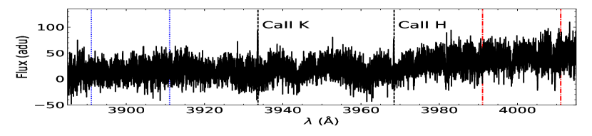
(a)

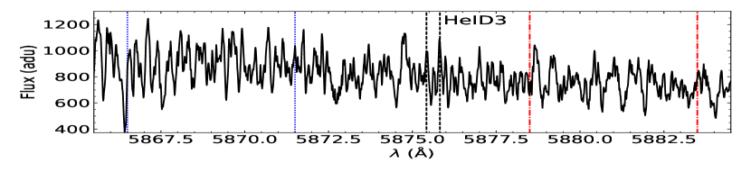
(b)

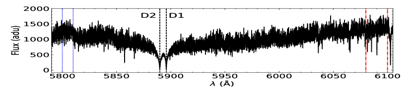
(c)

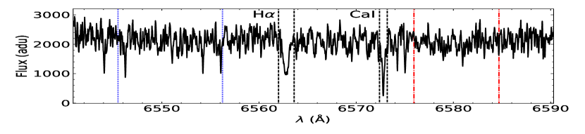
(d)

Figure 1: Region of the spectrum used to calculate activity indices for the CaII H&K, HeI, NaI, H$\alpha$ & CaI lines. The HARPS spectrum shown here was obtained on 25th January 2006. Within each figure, the blue and red vertical lines represent the reference continuum band used for each activity index. For HeI, H$\alpha$ & CaI, the black vertical lines represent the line bandwidths used for index calculations. For CaII H&K & NaI, the black vertical lines represent the respective line cores. Bandwidths used for line cores and reference continuum for each index calculation are mentioned in table 2.

3.1 CaII H&K

The CaII H&K lines are the most frequently explored magnetic activity proxy for solar-type stars (see, e.g., Baliunas et al., 1998). But for M dwarfs, their study could be challenging, since it requires longer exposure times due to their faint luminosity and low continuum levels (Scandariato et al., 2017). However, it provides significant information about the stellar chromosphere structure (Di Maio et al., 2020).

There were two spectral orders in our NARVAL dataset containing one of each of the H and K emission lines. Our spectra around these lines were relatively noisy, compared to the H$\alpha$ line, with a mean SNR of $\approx$ 11. The reduced spectra obtained from LIBRE-ESpRIT were not normalised well. We applied a re-normalisation procedure of fitting a 4th order polynomial to the continuum, from which, the spectral order containing the CaII H line was well normalised but the one containing the CaII K line was poorly normalised. Even after removing a few strong photospheric lines, the normalisation was not reliable (see Appendix B). We thus decided to study only the CaII H line for our NARVAL spectra defining our so called $I_{CaIIH}$ index following Morgenthaler et al. (2012) as

$$I_{CaIIH}=\frac{F_{CaIIH}}{F_{cont}}$$ (2)

where $F_{CaIIH}$ is the mean flux of the CaII H line within a 0.4Å wide rectangular window centered on 3968.47Å and $F_{cont}$ is the mean flux of the continuum within a 20Å wide rectangular window centered on 4001.07Å. The 0.4Å bandwidth was chosen as such to only encompass the CaII H emission line within it.

Since the continuum around the CaII H&K lines was relatively less noisy in the HARPS spectra, we calculate its CaII H&K index using $\tt ACTIN$ as

$$I_{CaII}=\frac{F_{CaIIK}+F_{CaIIH}}{F_{1}+F_{2}}$$ (3)

where $F_{CaIIK}$ & $F_{CaIIH}$ are the mean fluxes within a 1.09Å triangular window centered on 3933.664Å and 3968.47Å respectively and $F_{1}$ & $F_{2}$ are the mean fluxes within a 20Å square window centred on 3901.07Å and 4001.07Å respectively.

3.2 HeI D3

The HeI D3 line is observed to show presence of non-radiative heating mechanisms in cool stars (Landman, 1981) and can be used to investigate both the existence and variation of magnetic activity (Saar et al., 1997). The activity index is defined following Gomes da Silva et al. (2011) as

$$I_{HeI}=\frac{F_{HeI}}{F_{1}+F_{2}}$$ (4)

where $F_{HeI}$ is the mean flux within a 0.4Å wide bandwidth centered on the HeI D3 line 5875.62Å. $F_{1}$ & $F_{2}$ are the mean fluxes of the blue and red continuum centered on 5869Å & 5881Å and calculated within a bandwidth of 5.0Å respectively.

3.3 NaI

The NaI D resonance lines index is a good complement to the H$\alpha$ index since it represents the conditions of the middle-to-lower chromosphere as opposed to the upper chromosphere by H$\alpha$ (Mauas, 2000). We define our index following Díaz et al. (2007) as

$$I_{NaI}=\frac{f_{1}+f_{2}}{f_{cont}}$$ (5)

where $f_{1}$ & $f_{2}$ are the mean fluxes within a 1Å wide bandwidth centered on the D1 5895.92Å and D2 5889.95Å line cores. $f_{cont}$ is defined as the pseudo-continuum calculated as

$$f_{cont}=\frac{F_{1}+F_{2}}{2}$$ (6)

where $F_{1}$ & $F_{2}$ are the mean fluxes of the 10 highest flux values within two reference bands of width 10Å and 20Å centered on 5805Å and 6090Å respectively.

3.4 H$\alpha$

The H$\alpha$ line is sensitive to chromospheric activity and is extensively used as a standard activity tracer for M dwarfs (Linsky et al., 1982; West et al., 2004). In both the NARVAL and HARPS spectra, the H$\alpha$ line is in absorption since GJ 436 is a low activity M dwarf.

The standard approach of calculating the H$\alpha$ index is implemented following Boisse et al. (2009) as

$$I_{H\alpha}=\frac{F_{H\alpha}}{F_{1}+F_{2}}$$ (7)

where $F_{H\alpha}$ is the mean flux within a broad 1.6Å wide bandwidth centered on the H$\alpha$ line 6562.808Å. $F_{1}$ & $F_{2}$ are the mean fluxes of the blue and red continuum on either side of the line core within 10.75Å and 8.75Å wide bandwidths centered on 6550.87Å and 6580.31Å respectively.

3.5 CaI

The CaI line is observed a few angstroms to the right of the H$\alpha$ line at 6572.795Å and is known to not vary with stellar magnetic activity (Kürster et al., 2003). Because of this, we calculate the CaI index as a check for the H$\alpha$ activity significance since any variation in H$\alpha$ activity should not be seen in the CaI indices. The index is defined following Robertson et al. (2013) as

$$I_{CaI}=\frac{F_{CaI}}{F_{1}+F_{2}}$$ (8)

where $F_{CaI}$ is the mean flux of the CaI line in a 0.8Å wide window centered on the CaI line and $F_{1}$ and $F_{2}$ are the mean fluxes of the same continuum as that used for the $I_{H\alpha}$ index calculation in Sect. 3.4. The 0.8Å bandwidth was chosen to contain only the CaI line within it. The same spectral order used for the $I_{H\alpha}$ index calculation is used for calculating the CaI index. Each activity index time series figures are included in the supplementary material and are available online.

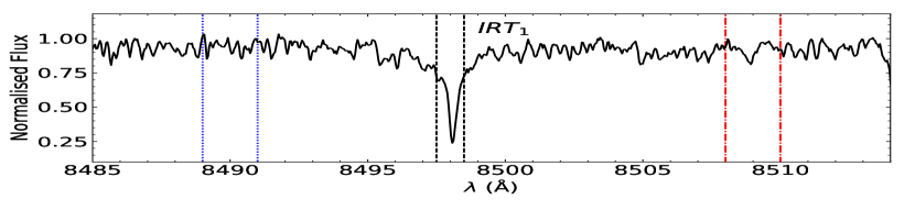
(a)

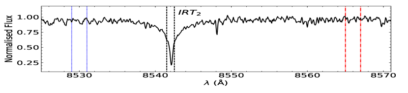
(b)

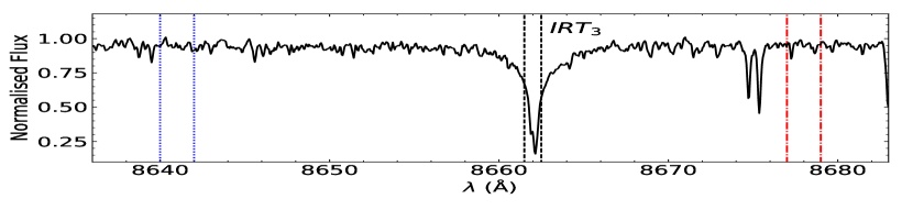
(c)

Figure 2: CaII IRT lines shown for one NARVAL spectrum obtained on 2nd June 2016. The blue and red vertical lines represent the reference continuum band and the black vertical lines represent the width of the line cores used for each IRT index calculation. Bandwidths used for these are detailed in table 2.

3.6 CaII IRT

The CaII IRT lines provide useful information about the middle chromosphere and can be used as an activity proxy for late-type main sequence stars (see, e.g., Mittag et al., 2017; Rutten, 2007). The HARPS spectra do not cover the CaII IRT lines. On the other hand, the NARVAL spectra do, since the spectropolarimeter has a wavelength coverage of 370 - 1000nm. We calculate the CaII IRT index for the 16 NARVAL spectra obtained in 2016.

The index for each of the three IRT lines is defined following Mittag et al. (2017) as

$$I_{IRT_{x}}=\frac{F_{IRT_{x}}}{F_{1}+F_{2}}$$ (9)

where $F_{IRT_{x}}$ is the mean flux of the line, $F_{1}$ & $F_{2}$ are the mean fluxes in the reference continuum bands. Here, $x$ = 1, 2, and 3, corresponds to each of the triplet lines at 8498Å, 8542Å & 8662Å respectively (see table 2). The $F_{IRT_{x}}$ mean fluxes are calculated within a 1Å wide bandwidth and the continuum mean fluxes within a 2Å wide bandwidth.

Table 3 and 4 contain the values for each calculated index along with their errors for the HARPS and NARVAL spectra respectively.

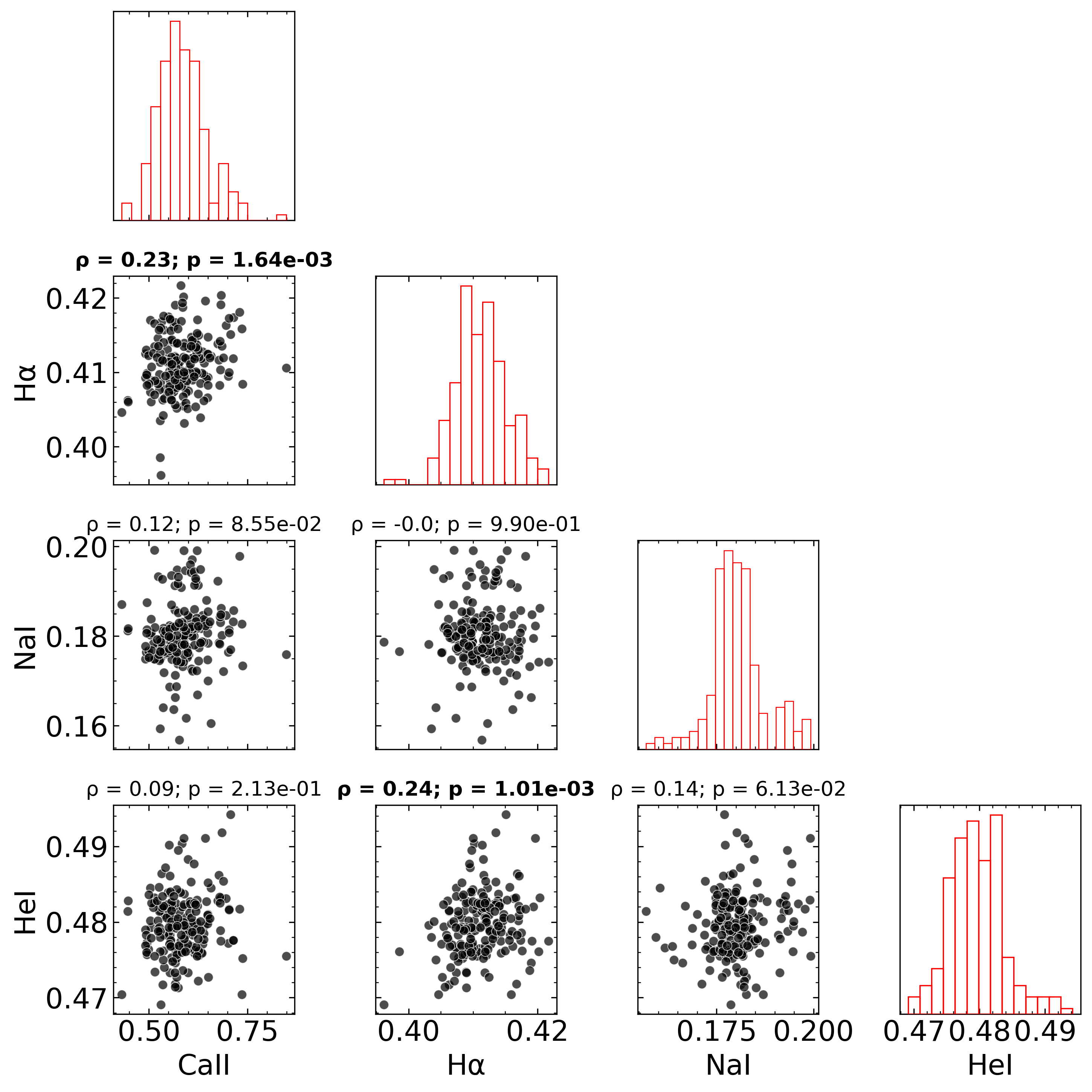
Figure 3: Corner plot showing correlations between the four activity indices CaII H&K, HeI NaI, and H$\alpha$, for 192 HARPS spectra. The diagonal panels show the histogram distribution of each index. The Pearson R correlation coefficient ($\rho$) and its p-value are shown above each correlation plot, with significant correlation values shown in bold.

Table 5: Pearson R correlation between activity indices per epoch. For each correlation, the shown results are [$\rho$, p-value, (slope)] where $\rho$ is the correlation coefficient, p-value is the corresponding null-hypothesis probability and slope is the slope of its best-fit line. Correlations with their p-value < 0.05 are shown in bold. For the 2016 (NARVAL) epoch, values are shown for correlations with CaII H instead of CaII H&K.

Epoch	H$\alpha$ vs CaII H&K	H$\alpha$ vs NaI	NaI vs CaII H&K	CaII H&K vs HeI	H$\alpha$ vs HeI	NaI vs HeI
2006	0.4506, 0.3103, (6.2344)	-0.6655, 0.1028, (-0.9041)	-0.2644, 0.5667, (-2.6923)	-0.5022, 0.2508, (-0.0546)	-0.4812, 0.2743, (-0.7233)	0.4285, 0.3375, (0.4741)
2007	0.3459, 0.0045, (7.4930)	0.1785, 0.1516, (0.3953)	0.1066, 0.3945, (1.0424)	-0.0395, 0.7529, (-0.0026)	0.1627, 0.1919, (0.2314)	0.0299, 0.8117, (0.0192)
2008	0.0921, 0.5380, (0.9013)	-0.2896, 0.0483, (-0.3309)	0.2925, 0.0460, (2.5049)	-0.0342, 0.8194, (-0.0031)	-0.1256, 0.4003, (-0.1129)	0.2690, 0.0680, (0.2117)
2009	0.1514, 0.3512, (1.7055)	0.1718, 0.2891, (0.1974)	0.0087, 0.9577, (0.0850)	0.1208, 0.4580, (0.0125)	0.5898, 0.00006, (0.6853)	-0.0361, 0.8248, (-0.0365)
2010	0.8977, 0.0010, (20.5098)	-0.3035, 0.4273, (-0.3232)	-0.0264, 0.9462, (-0.5665)	0.5106, 0.1601, (0.0289)	0.6501, 0.0580, (0.8392)	-0.6982, 0.0365, (-0.8462)
2016	-0.1290, 0.7060, (-4.1041)	0.1507, 0.5862, (0.3671)	-0.612, 0.0117, (-7.9959)	-0.3390, 0.1990, (-0.0184)	0.1794, 0.5063, (0.3094)	0.1850, 0.4927, (0.1311)
2020	0.2235, 0.3054, (2.7487)	0.0948, 0.6669, (0.0819)	-0.0151, 0.9454, (-0.2154)	0.2237, 0.3049, (0.0211)	-0.0946, 0.6678, (-0.1098)	0.0617, 0.7799, (0.0829)

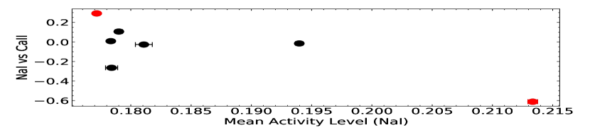
(a)

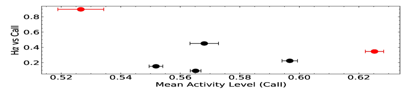
(b)

Figure 4: Correlation coefficients ($\rho$) plotted against the mean activity level per observing epoch for 2 pairs of index correlations. For H$\alpha$ vs CaII, we only plot the HARPS epoch correlations since we calculate a CaII H index for the NARVAL epoch. In each plot, the red dot markers are correlation coefficients with p-value < 0.05.

4 Correlation between indices

In this section, we explore linear correlations between the CaII H&K, HeI, NaI, CaII IRT, and H$\alpha$ indices, each representing the lower, mid-to-lower, middle and upper chromosphere respectively. Additionally, we compare the CaI line index to the H$\alpha$ index to see whether it correlates with an index insensitive to magnetic activity. The linear correlations are studied using the Pearson R correlation coefficient with correlations considered significant if their null-hypothesis probabilities, i.e. p-values, are < 0.05. We remind the reader here that for the NARVAL dataset, the CaII H index was calculated instead of CaII H&K.

4.1 Correlations for HARPS dataset

We begin by analysing the full HARPS dataset covering $\approx$ 14 years. Figure 3 shows a corner plot with correlations for each of the 4 activity indices. Each subplot has its respective Pearson R correlation coefficient and the p-value shown above it.

We found the CaII H&K indices to show a weak positive correlation with the H$\alpha$ indices with a coefficient of 0.23 (p=0.0016). Furthermore, the HeI index showed a significant positive correlation with the H$\alpha$ index with a coefficient of 0.24 (p=0.0010).

The correlation between CaI and H$\alpha$ indices was found to be insignificant with a coefficient of -0.07 (p=0.318).This shows that the variations in H$\alpha$ indices are real, since the CaI line is insensitive to stellar activity.

4.2 Correlations per Epoch

In order to study how these correlations vary over long-term, and the effect of a possible cycle on them, we analyze separately the activity index correlations from each observing epoch of the HARPS dataset. Here, we treat the NARVAL dataset as an epoch along with the six HARPS epochs, with each having a mean timespan and number of data points of $\approx$ 90 days and 30 respectively. The correlation coefficients per epoch along with their p-values, are listed in table 5 for both NARVAL and HARPS dataset with significant correlations shown in bold. Corner plots showing correlations per observing epoch are included in the supplementary material and are available online.

Out of the 7 observing epochs, two epochs showed a significant correlation between the H$\alpha$ and CaII H&K indices as shown in table 5. The correlation coefficient in the 2010 epoch is roughly 2.6 times higher than that in the 2007 epoch. The NaI vs CaII H&K index showed a significant correlation for 2 epochs as well. However, their correlation switches from positive, in 2008, to negative, in 2016. The absolute value of their correlation coefficient nearly doubles between these epochs. All of these results demonstrate that activity index correlations for GJ 436 vary with time.

In addition to these correlations, for the epoch of observations done with NARVAL, we found the CaII IRT indices to show significant correlations for IRT₂ vs IRT₃ & H$\alpha$ vs IRT₃ with their correlation coefficients being -0.56 (p=0.024) & -0.54 (p=0.031) respectively.

We further investigate whether the correlations change with the level of stellar activity. For that, we study the correlation coefficient variation as a function of the mean activity level (MAL) of each epoch, for the indices that show a significant correlation in at least two epochs of observation. The error on MAL is calculated using error propagation. As shown in figure 4, the NaI vs CaII & H$\alpha$ vs CaII index correlation coefficients tend to show a general trend of decreasing with increasing MAL of NaI & CaII per epoch respectively. If only the significant correlations are considered, shown with the red dot markers, the trend remains the same.

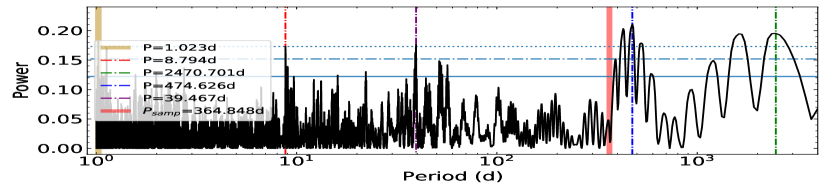
(a)

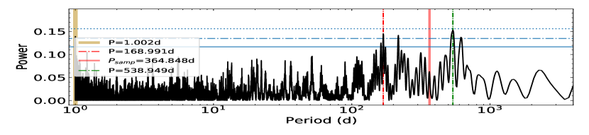
(b)

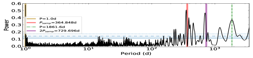
(c)

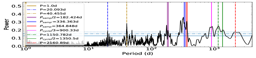
(d)

Figure 5: GLS periodogram of the CaII H&K (top left), HeI (top right), NaI (bottom left) and H$\alpha$ (bottom right) indices with the x-axis showcasing the trial periods in logarithmic scale. Periods with FAP < 0.1% are considered significant and shown using vertical coloured dash-dot lines with their respective periods mentioned in the plot legend of each periodogram. For HeI, the plot legend shows periods with FAP < 1%. The thick coloured vertical lines show the three sampling window periods detected from the sampling window function periodogram. In the H$\alpha$ periodogram, the colored solid lines show the integer harmonics of the 7.4 years photometric activity cycle. The solid, dash-dot and dotted blue horizontal lines show the false alarm levels for 10%, 1% and 0.1% respectively.

5 Variability of Activity indices

In the following, we investigate the short and long-term periodicity of activity indices in order to study the stellar rotation period as well as a possible long-term activity cycle. Recently, an activity cycle of 7.4 years was reported for GJ 436 in photometry (Lothringer et al., 2018), and here we explore if it is detectable in spectroscopy.

5.1 Generalised Lomb-Scargle (GLS)

For our analysis, we use the Generalised Lomb-Scargle (GLS) method (Zechmeister & Kürster, 2009). Effectively sampled period grid ranging from 1d to 4000d is used in order to cover at least one oscillation of the 7.4 years activity cycle. The false alarm probability (FAP) of each detected period is estimated using the ’bootstrap’ method (Kuerster et al., 1997). The error on each detected period is determined from the full width at half maximum (FWHM) of its respective power peak in the periodogram. Periods detected with FAPs < 0.1 % are considered significant.

For HeI, NaI & H$\alpha$, we combine the indices from the HARPS & NARVAL datasets. The NARVAL 2016 observations fill a gap in the 14 years of HARPS observations. For CaII H&K indices, we use the HARPS dataset alone, since this index is not calculated for NARVAL (see section 3.1). Figure 5 shows the periodograms for CaII H&K, HeI, NaI & H$\alpha$ indices. Periodograms per observing epoch for each of these indices are included in the supplementary material and are available online.

5.1.1 CaII H&K

From the periodogram of CaII H&K indices, shown in figure 5, we detect a period of $474.6^{+14.8}_{-24.5}$d with the highest peak in power. The next best period is 2470.7d, roughly 6.8 years, with a relatively large FWHM. In addition to these, we detect two short periods of $39.47^{+0.11}_{-0.15}$d and $8.79^{+0.02}_{-0.01}$d.

We detect a strong peak around 1 day. This period is identified as a direct result of our sampling window function (see Appendix C). Along with that, we detect a period of $364.8^{+5.2}_{-6.3}$d ($P_{samp}$ from hereon). This period is possibly a result of long term observations, with data collected each year. It should be noted that we do not detect it in the CaII H&K periodogram with a significant FAP. Both $P_{samp}$ and the 1d sampling periods are shown in figure 5 with red and gold thick lines respectively.

Running the periodogram analysis on each observing epoch individually, we detect periods of $43.2^{+7.8}_{-4.6}$d and $48.6^{+12.2}_{-7.2}$d from the 2007 & 2008 epochs respectively. These periods are in good agreement with the $39.47^{+0.11}_{-0.15}$d period detected from the combined HARPS & NARVAL datasets. From the 2009 epoch, we detect two periods of 87.27d, with a relatively large FWHM, and $21.9^{+1.3}_{-1.4}$d. We detect a short period of $2.82^{+0.04}_{-0.07}$d from the 2008 epoch as well .

5.1.2 NaI

From the periodogram of NaI indices, shown in figure 5, we detect a period of $351.9^{+6.0}_{-9.4}$d with the highest peak in power, after the 1d sampling window period. However, this period is 3.6 % shorter than $P_{samp}$, shown with the red thick line, and is not considered a true period. Another significant period of $699.3^{+23.3}_{-27.1}$d is detected which is roughly twice $P_{samp}$ and hence not considered a true period. In addition to these, a period of 1861.6d, roughly 5.1 years, is detected as well.

Running the periodogram analysis on each observing epoch individually, we detect a period of $46.9^{+11.9}_{-6.1}$d from one epoch only, the 2008 epoch. However, we detect shorter periods of $14.90^{+0.78}_{-0.58}$d and $14.92^{+0.82}_{-0.70}$d from the 2008 and 2016 epochs, respectively.

5.1.3 H$\alpha$

From the periodogram of H$\alpha$ indices, shown in figure 5, we detect a period of $321.3^{+27.0}_{-14.6}$d with the highest peak in power. But like for NaI, this period is 4.5% shorter than the sampling window period of $336.4^{+5.7}_{-8.1}$d (see Appendix C) and, within its error bars, is most probably due to our sampling window. We detect the $P_{samp}$ period along with its $2^{nd}$ integer harmonic, $P_{samp}$/2, shown using appropriate thick coloured lines in the periodogram. In addition to these, we detect two short periods of $40.46^{+0.44}_{-0.52}$d and $20.09^{+0.04}_{-0.05}$d, with the latter being a possible $2^{nd}$ integer harmonic of 40.46d.

We detect the $2^{nd}$ and $3^{rd}$ integer harmonics of the 7.4 year activity cycle, shown using appropriate thick coloured lines in the periodogram, along with 2 distinct periods of 1150.8d and 2160.9d, with a relatively large FWHM. Like for CaII H&K and NaI, the 1d sampling window period is detected as well.

Running the periodogram analysis on each observing epoch individually, we detect a period of $42.1^{+2.0}_{-4.3}$d and $44.1^{+8.1}_{-5.5}$d from the 2007 & 2009 epochs respectively. From the 2008 epoch, we detect two notable short periods of $50.3^{+8.7}_{-4.9}$d and $19.85^{+0.77}_{-0.93}$d.

5.1.4 HeI

From the periodogram of HeI indices, shown in figure 5, we do not detect any periods with FAPs < 0.1%. However, we do detect 2 distinct periods with FAPs < 1%. These periods are $538.95^{+20.08}_{-27.51}$d & $168.99^{+2.28}_{-2.03}$. We detect the sampling window period of 1d as well. Unlike the other indices, we do not detect any significant long-term periods.

Running the periodogram analysis on each observing epoch individually, we do not detect any periods with FAPs < 0.1%.

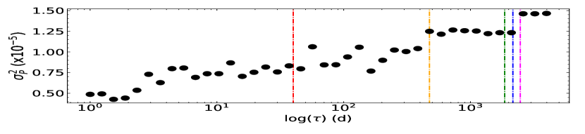
(a)

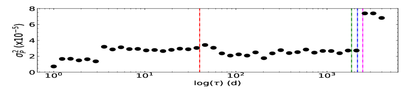
(b)

Figure 6: Pooled variance of H$\alpha$ (left) and NaI (right) indices calculated from both HARPS and NARVAL datasets. The x-axis shows timescales ($\tau$) in logarithmic scale ranging from 1d to 4000d. In both the figures, the red vertical line represents the stellar rotation period of 40d detected from the H$\alpha$ and CaII H&K periodogram. The green, blue and magenta lines represent the longest periods of 1861.6d, 2160.9d and 2470.7d detected from periodograms of NaI, H$\alpha$ and CaII H&K indices respectively. The orange vertical line in the left figure represents the 474.6d period detected from the periodogram of CaII H&K indices (see section 5.1.1)

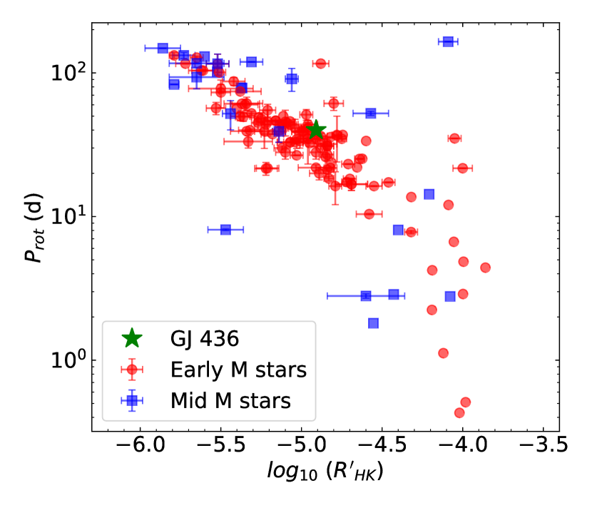
Figure 7: Chromospheric activity level $log_{10}R^{\prime}_{HK}$ plotted against the stellar rotation periods of 112 M dwarfs. The red dot markers are the early M-type stars ranging from M0 - M3. The blue square markers are the mid M-type stars ranging from M3.5 to M6. The green star marker represents our star GJ 436 with its $P_{rot}$ equal to 40d and its $log_{10}R^{\prime}_{HK}$ calculated as -4.909 from the CaII H& indices. The data used to create this figure is taken from (Suárez Mascareño et al., 2018; Astudillo-Defru et al., 2017; Suárez Mascareño et al., 2017, 2016, 2015)

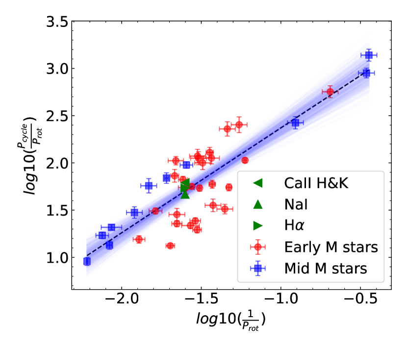
Figure 8: $log10(\frac{1}{P_{rot}})$ plotted against $log10(\frac{P_{cycle}}{P_{rot}})$ for 38 M dwarfs. The red dot markers are the early M-type stars ranging from M0 - M3 and the blue square markers are the mid M-type stars ranging from M3.5 to M6. The green triangle markers represent the long-term periods of 2470.7d, 1861.6 and 2160.9d detected from the periodograms of CaII H&K, NaI and H$\alpha$ indices respectively. The $P_{rot}$ is equal to 40.0d in all three cases. The dashed black line represents the best-fit line and the blue lines shape a band depicting the 95% confidence interval of the best-fit line. The data used to create this figure is taken from (Suárez Mascareño et al., 2018; Suárez Mascareño et al., 2016)

5.2 Prewhitening

Table 6: Table containing the detected periods from GLS periodograms of CaII H&K & H$\alpha$ indices after applying the prewhitening technique. The original short-term periods detected from both of these indices is mentioned once in red and blue bold colours. The detected periods similar to the original periods are shown using the same bold colours as well. FAPs for all periods are shown within brackets next to them.

Prewhitened Period (d)	Detected Periods (d)	Original Period (d)
	CaII H&K
474.63 (< 0.1%)	$9.68^{+0.03}_{-0.01}$ (< 1%)	$\mathbf{39.47^{+0.11}_{-0.15}}$ (< 0.1%)
	$32.36^{+0.33}_{-0.3}$ (< 1%)	$\mathbf{8.79^{+0.02}_{-0.01}}$ (< 0.1%)
	8.80 ± 0.03 (< 1%)
2470.70 (< 0.1%)	$9.68^{+0.03}_{-0.01}$ (< 0.1%)
	8.80 ± 0.03 ($\approx$ 0.1%)
	$102.80^{+3.04}_{-4.80}$ (< 1%)
	$80.00^{+1.60}_{-2.11}$ (< 1%)
	$\mathbf{38.81^{+1.40}_{-0.64}}$ (< 10%)
	H$\alpha$
1150.78 (< 0.1%)	$137.12^{+1.33}_{-1.2}$ (<0.1%)	$\mathbf{40.46^{+0.44}_{-0.52}}$ (< 0.1%)
	$48.96^{+0.17}_{-0.23}$ (< 0.1%)	$\mathbf{20.09^{+0.04}_{-0.05}}$ (< 0.1%)
	$173.53^{+1.93}_{-1.91}$ (< 0.1%)
	$55.06^{+0.22}_{-0.19}$ (< 0.1%)
	$\mathbf{19.99^{+0.12}_{-0.11}}$ (< 0.1%)
	$\mathbf{40.46^{+0.23}_{-0.66}}$ ($\approx$ 1%)
2160.89 (< 0.1%)	$137.00^{+1.46}_{-1.35}$ (< 0.1%)
	$189.10^{+2.63}_{-4.70}$ (< 0.1%)
	$\mathbf{20.0^{+0.13}_{-0.11}}$ (< 0.1%)
	$\mathbf{40.43^{+0.15}_{-0.80}}$ (< 0.1%)

With a focus on inspecting whether the short-term periods detected from the periodograms of CaII H&K and H$\alpha$ indices, in section 5.1, are detectable in the absence of their respective long-term periodicity, we perform a prewhitening procedure on our indices. Following Blomme et al. (2011), we fit a sine wave function to the index time series, with a period equal to the long-term period. The fitted sine function is then subtracted from the index time series and a GLS periodogram is run on this "prewhitened" data to reassess its short-term periodicity. When multiple long-term periods are detected in a periodogram, we apply the prewhitening procedure on each of these periods separately.

For the CaII H&K indices, two long-term periods of 474.63d and 2470.7d are detected in the GLS periodogram. When we prewhiten the 474.63d period, we detect a short-term period of 32.36d, which is $\approx$ 18% shorter than the original period of 39.47d. When prewhitening the 2470.7d period, we detect a period of $38.81^{+1.40}_{-0.64}$d. This period, within its error bars, is comparable to the 39.47d period detected from the non-prewhitened CaII H&K indices but with a larger FAP of < 10%.

For the H$\alpha$ indices, we prewhiten the 1150.78d period and from the resultant periodogram, we detect a period of $40.46^{+0.23}_{-0.66}$d. This period is exactly the same as the original 40.46d period detected from the non-prewhitened H$\alpha$ indices but has a different FAP of $\approx$ 1% instead of < 0.1%. When we prewhiten the long-term period of 2160.89d, we detect a period of $40.43^{+0.15}_{-0.80}$d. This period, within its errors bars, is comparable to the 40.46d period with both having the same FAP of < 0.1%.

Table 6 shows all of the detected periods after prewhitening for both CaII H&K and H$\alpha$ indices with detected periods similar to the original period shown in red and blue bold colours.

5.3 Pooled Variance Analysis

In order to further investigate the long-term periodicity of our activity indices, we implemented the "Pooled Variance" (PV) technique (Lanza et al., 2004; Donahue et al., 1997a, b). The PV is calculated by binning our data into evenly-spaced bins with some timescale length $\tau$. The mean of the variance from each bin for a given $\tau$ is the PV for that $\tau$. Changes in the PV for different timescales are assumed to be associated with several mechanisms such as stellar rotation, the lifetime of possible Active Region (AR), and long-term activity cycles. The PV technique can thus be used to identify the approximate timescales at which a given activity mechanism dominates. We apply PV to NaI & H$\alpha$ indices. We do not apply it to CaII H&K indices, because CaII H&K indices were not calculated for NARVAL (see section 3.1), and thus the gap in our data is of 10 years. HeI does not show any significant long-term periodicity for us to investigate it further. Figure 6 shows the PV diagrams for H$\alpha$ (left) and NaI (right) indices for timescales ranging from 1d to 4000d.

For H$\alpha$ indices, the PV diagram at shorter timescales increases steadily. Near the stellar rotation timescale of 40d, shown using the red vertical line in figure 6, the PV appears to be relatively constant over a short timescale range. Eventually, the PV reaches a plateau starting at $\approx$ 470d which could be related to the lifetime of potential AR complexes for GJ 436. This period fits well within the range of AR lifetimes observed for slow M rotators (Giles et al., 2017). This timescale is comparable to the period of 474.6d as well, detected from the periodogram of CaII H&K indices (see section 5.1.1), shown using the orange vertical line. At timescales greater than 1000d, we observe a sharp increase in the PV reaching another plateau starting at $\approx$ 2500d. This PV increase is likely due to a possible activity cycle. To compare it with the long-term periods detected from section 5, we show the periods of 1861.6d, 2160.9d & 2470.7d, detected from NaI, H$\alpha$ & CaII H&K periodograms respectively, using appropriately coloured vertical lines in figure 6. The 2470.7d period detected from the CaII H&K periodogram, being close to the period of 2160.9d detected from the H$\alpha$ periodogram, falls near the start of the activity cycle plateau and is in good agreement with the $\approx$ 2500d period.

For NaI indices, the PV diagram remains constant for timescales up to 3d and then nearly doubles. With increasing timescales, the PV remains constant until a timescale close to the stellar rotation where it slightly decreases to eventually have a sharp peak at the timescale of $\approx$ 2500d.

6 Discussion

In this paper, we studied the chromospheric activity of GJ 436 using data collected over 14 years by the HARPS spectrograph and the NARVAL spectropolarimeter (spanning 85 days), with the NARVAL data falling within the 14 years of HARPS observations. We analysed six different spectral lines: CaII H&K, HeI, NaI, H$\alpha$ CaI and CaII IRT, and the correlations between them. We explored the periodicity of these indices, both on a short and long time-scale.

6.1 Index Correlations

From the long time span HARPS dataset, we found the CaII H&K indices to show a weak positive correlation with the H$\alpha$ indices. The HeI index was found to show a weak positive correlation with the H$\alpha$ index as well. In order to explore how these correlations change over time, they were studied for each of the six observing epochs of HARPS , as well as the 2016 epoch of NARVAL.

For two pairs of correlations, we found at most two observing epochs which showed significant correlations, i.e. with p-values less than 0.05. The coefficient of correlation for these pairs seem to be decreasing with the mean activity level of the star (calculated for one of the activity indices), shown in figure 4. However, we have only 2 significant correlations for each of these correlation pairs, and caution the reader that this trend needs further confirmation. The differences in correlation between epochs could be due to different phases of an activity cycle (see, e.g. Scandariato et al., 2017; Meunier & Delfosse, 2009). In fact, GJ 436 has a reported photometric activity cycle of 7.4 years (Lothringer et al., 2018). Gomes da Silva et al. (2011), when studying long term activity of a sample of M dwarfs, found the correlations to vary with the level of stellar activity. Change of correlation between indices is reported for the Sun as well (Maldonado et al., 2019), with these changes being attributed to the variation of the concentration of plages and dark filaments on the solar surface.

From the H$\alpha$ vs CaII plot in figure 4, we found a strong positive correlation of 0.9 at the lowest mean activity level of the CaII indices. The CaII lines are more sensitive to the surface coverage of plages than the H$\alpha$ line, which is sensitive to dark filaments (Meunier & Delfosse, 2009; Gomes da Silva et al., 2011). The existence of plages and dark filaments in the same location on the stellar surface could thus account for the strong positive correlation, occurring in the 2010 observing epoch.

From the 2016 NARVAL epoch, we found the CaII IRT₃ to correlate negatively with the CaII IRT₂. The IRT₃ showed a negative correlation with the H$\alpha$ index as well.

6.2 Stellar Rotation Period

Using the combined HARPS and NARVAL dataset, we detected short-term periods of $39.47^{+0.12}_{-0.15}$d and $40.46^{+0.44}_{-0.52}$d from the variations of CaII H&K and H$\alpha$ activity indices respectively. Both periods have FAPs < 0.1 % and are considered significant. These periods are interpreted as the rotation periods of GJ 436 and are in good agreement with the 39.9 ± 0.8d period found by Suárez Mascareño et al. (2015) in the variations of $log_{10}(R^{\prime}_{HK})$ and the 42.6 ± 2.2d period found by Bourrier et al. (2018) in the variations of H$\alpha$ indices. Exploring periodicity in each of the 7 observing epochs individually, we detected periods of $43.2^{+7.8}_{-4.6}$d & $48.6^{+12.2}_{-7.2}$d from CaII H&K and $42.1^{+2.0}_{-4.3}$d & $44.1^{+8.1}_{-5.5}$d from H$\alpha$ indices in 2 separate observing epochs. These periods, within their error bars, are compatible with the ones found from the whole dataset. To further test the effect of long-term periodicity on the detection of these rotation periods, we prewhitened the long-term periods (see section 5.2) for the CaII H&K and H$\alpha$ indices. We detected the rotation periods in the prewhitened data as well, with varying FAPs, showcasing that these periods are thus significant and not aliases of the long-term periodicity.

Considering the B - V color of GJ 436, these derived $P_{rot}$ periods fall within the expected range of detected rotation periods for early M dwarfs of spectral type M0-M3 (see figure 10 in Suárez Mascareño et al., 2018). These periods are consistent with the rotation periods of M dwarfs with stellar masses similar to GJ 436 as well (see figure 10 in Newton et al., 2017). From this figure, our star falls within the inactive M dwarfs branch. To compare our mean $P_{rot}$ of 40.0d from the variations of CaII H&K and H$\alpha$ indices to other M dwarfs, we calculated a mean $log_{10}(R^{\prime}_{HK})$ for GJ 436 and plot it against the stellar rotation periods of 112 M dwarfs (Suárez Mascareño et al., 2018; Astudillo-Defru et al., 2017; Suárez Mascareño et al., 2017, 2016, 2015), ranging in spectral type from M0 - M3 (see fig.7). GJ 436 falls within the trend of the M dwarfs of similar rotation periods and activity levels, within the unsaturated regime of the rotation-activity relation.

From the NaI index variations we detect a period of $46.9^{+11.9}_{-6.1}$d, from the 2008 observing epoch, compatible with the ones detected from CaII H&k and H$\alpha$ indices. From the 2016 observing epoch, we detect a period of $14.92^{+1.23}_{-0.98}$d comparable to $\approx$ $\frac{1}{3^{rd}}$ of $46.9^{+11.9}_{-6.1}$d, within its error bars.

6.3 Activity Cycle Period

The CaII H&K, NaI & H$\alpha$ indices show significant long-term periodicity, which one might expect given the reported photometric activity cycle of 7.4 years (Lothringer et al., 2018). The indices show long-term variations with periods of 2470.7d, 1861.6d & 2160.9d, which are roughly 6.8 years, 5.1 years and 5.9 years respectively. Additionally, we detect a period of $474.6^{+14.8}_{-24.5}$d from the CaII H&K index variations. From the H$\alpha$ index variations, we detect the $2^{nd}$ and $3^{rd}$ integer harmonics of the photometric activity cycle as well with periods 1350.5d and 900.3d respectively.

We reassessed the long-term periodicity of H$\alpha$ and NaI indices using the "Pooled Variance" technique which indicates the lifetime of an activity cycle to be $\approx$ 2500d. This is in good agreement with the long-term period of 2470.7d detected from the CaII H&K periodogram. We compare our derived cycle periods to other M stars to place them in the perspective of early M dwarfs. Using 40.0d as our derived $P_{rot}$, we compare $log_{10}$ of $\frac{P_{cycle}}{P_{rot}}$ against $log_{10}$ of $\frac{1}{P_{rot}}$ for 38 M dwarfs. Here, $P_{cycle}$ are the three long-term periods derived from the CaII H&K, NaI & H$\alpha$ index variations. As shown in figure 8 with appropriate green triangle markers, our derived $P_{cycle}$ periods fall within the 95% confidence interval of the best-fit line. Considering the color in this case, our derived $P_{cycle}$ periods show similar values to those of M0 - M3 type M dwarfs (see figure 11 in Suárez Mascareño et al., 2018).

7 Conclusion

From our results, we detect the stellar rotation period of GJ 436 from the variations of spectroscopic activity indicators. Suárez Mascareño et al. (2018) find a mean stellar rotation & activity cycle period of 33 ± 23 d & 6.3 ± 3.4 years respectively, for M0 - M3 type M dwarfs, with both our $P_{rot}$ and $P_{cycle}$ periods falling within these expected ranges. Additionally, we find that the correlations between activity indices vary with the level of stellar activity over time.

The activity of GJ 436 could be following a long-term cycle, compatible with the photometric one. However, in order to better determine the cycle period, further data with denser spectroscopic monitoring are needed. Understanding magnetic activity and cycles in M-dwarfs is a crucial step in filtering the activity RV signature, which would help confirm additional planets in a system, if present. Furthermore, a better understanding of chromospheric activity cycles of GJ 436 is necessary in studying the impact of its stellar activity on the atmosphere and potential habitability of its hot-Neptune GJ 436b, which is one of the prime targets for multiple James Webb Space Telescope Guaranteed Time Observations (GTO) programs as well as other space missions such as ARIEL (Edwards & Tinetti, 2022).

Data Availability

This paper uses data based on observations collected at the European Southern Observatory under ESO programs 072.C-0488(E), 082.C-0718(B), 183.C-0437(A), 1102.C-0339(A) and 1102.C-0339(F), using the HARPS spectrograph. Additionally, it uses data from the Pic du Midi Observatory, for the program L161N04, using the NARVAL spectropolarimeter.

The Python code used to calculate the activity indices is publicly available on https://github.com/MXK606/krome. The data used in this paper are publicly available on ESO archive (http://archive.eso.org/scienceportal/home) for HARPS data, and on Polarbase database (http://polarbase.irap.omp.eu) for NARVAL data with additional figures available as online supplementary material.

Appendix A H$\alpha$ index method comparison

From the NARVAL dataset for comparison, in addition to the standard method in section 3.4, we adopted the method of Gomes da Silva et al. (2011) for calculating the H$\alpha$ index where instead of mean in equation 7, each flux was calculated as a sum over their respective bandwidths. Additionally, following Jeffers et al. (2018), we calculated the pseudo-Equivalent Width (pEW) of the H$\alpha$ absorption line as well to compare with the H$\alpha$ index as

$$pEW=\int_{\lambda_{1}}^{\lambda_{2}}(1-\frac{F(\lambda)}{F_{pc}})\,d\lambda\$$ (10)

where $F_{pc}$ is defined as the mean of the median flux in the so called pseudo-continuum within the spectral ranges (6545.0Å - 6559.0Å) and (6567.0Å - 6580.0Å). For our star, the pEW value was measured within a narrower 1.6Å wide bandwidth from (6562.008Å - 6563.608Å) centered on the H$\alpha$ line than the one used by Jeffers et al. (2018). The error on $pEW$ was calculated following Jeffers et al. (2018).

The H$\alpha$ activity index in literature is calculated simply using equation 7. But, each flux in this equation is calculated differently by different authors. Boisse et al. (2009) calculated each flux as the mean flux value within the respective bandwidth for its target HD 189733. Similarly, Boro Saikia et al. (2016) calculated the flux as the mean flux value as well for its target HD 201091. Robertson et al. (2013) however calculated each flux as the sum of the flux values for its (K5-M5) dwarf sample and Gomes da Silva et al. (2011) did the same for its (M0-M5.5) dwarf sample.

To check how these methods vary with one another, we compared the mean and the sum method of calculating the H$\alpha$ index by calculating its Pearson R correlation coefficient. We found their R coefficient to be 0.99 with a p-value of $5\times 10^{-13}$, which is the probability of finding the same coefficient for a null hypothesis. Both of these index methods were found to correlate positively as shown in figure 9 with the mean method producing indices $\approx$ 6 times larger than the sum method. This is simply because the sum method of index calculation is sensitive to the number of flux points in each bandwidth as opposed to the mean method and the H$\alpha$ line core bandwidth is much smaller than the reference continuum bandwidths leading to a relatively smaller sum index value. But for studying stellar activity variations, either of these methods could be employed since they both show a strong positive linear correlation.

The H$\alpha$ index (mean method) is then compared to the pEW and their Pearson R correlation coefficient is found to be -0.99 (p-value=$2\times 10^{-12}$). These two methods are found to correlate negatively as shown in figure 9. The H$\alpha$ index and the pEW methods are both calculated within the same bandwidth of 1.6Å. centered on the H$\alpha$ line apart from the continuum reference bands. This shows that as the mean flux within the H$\alpha$ line increases thereby increasing the H$\alpha$ index, its relative pEW decreases, as expected.

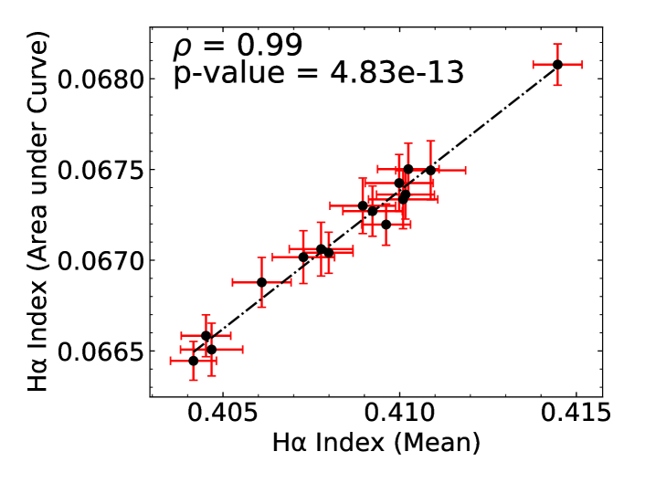
(a)

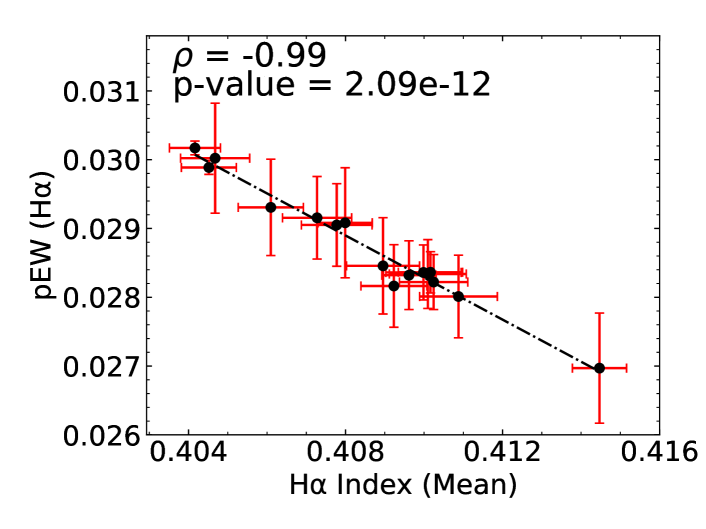
(b)

Figure 9: Correlation between the H$\alpha$ index calculated from the NARVAL dataset using the mean and the sum method (top) & between H$\alpha$ index (mean method) and the pEW (bottom). The dash-dotted line shows the best-fit line and $\rho$ is the Pearson R correlation coefficient. The corresponding error bars for each index are plotted in red.

Appendix B NARVAL spectral orders around Calcium II H&K

The NARVAL data reduced by the data reduction software LIBRE-ESpRIT contains 40 individual spectral orders numbered from #22 to #61. These orders overlap with one another at their respective borders, as shown in figure 10. The figure shows the spectral order containing the CaII K line to be noisier than the order containing the CaII H line. In order to calculate the CaII H&K activity index for our star, these spectral orders need to be re-normalised to unit flux. Each spectral order was fitted to a 4th order polynomial using the astropy package $\tt specutils$ (Earl et al., 2021). The order was then divided by this polynomial fit to give the re-normalised spectra. For the blue order containing the CaII K line, 2 strong emission lines at 3931.6Å and 3924.2Å were removed by fitting a Gaussian to them and subtracting the Gaussian fit from the entire spectra. The removal of these lines did not affect the re-normalisation process and the order containing the CaII K line was not well normalised. The reason this order looks this way after the re-normalisation procedure is due to large number of negative flux values encountered in the wavelength range of 3900 - 3950 Å. Thus when this region of the order is divided by a constant polynomial fit, which for this region has values close to zero, it stretches the spectra vertically in such fashion. Hence, only the CaII H line was analysed in section 2.

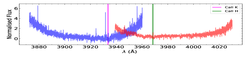
(a)

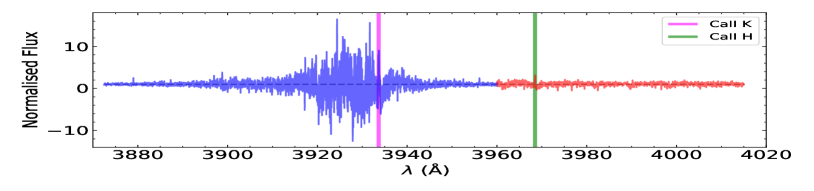
(b)

Figure 10: Pipeline normalised spectra (top) and the re-normalised spectra (bottom) for the two spectral orders around the CaII H&K emission lines of the 16th March 2016 NARVAL observation. The blue spectral order contains the CaII K line and the red spectral order contains the CaII H line. The gray dashed line in the bottom plot shows the flux level at unity.

Appendix C Computing the window function to check for sampling biases in periodogram

For unevenly sampled data, often times the true period peak is surpassed in power by spurious period peaks. Such peaks can be seen in the periodograms in figure 5. One major factor leading to these peaks is the duration between the observations (VanderPlas, 2018).

To confirm this, we compute the window function of our observations by setting our $y_{n}$ and $dy_{n}$ values equal to 1 for all times $t_{n}$ and run a classical periodogram on them with the values not pre-centered. The resulting periodogram, shown in figure 11, shows a peak at P=1d which is a common occurrence for ground-based surveys as the observations are done almost at the same time every other night. In addition to this, we detect a period of $364.8^{+5.2}_{-6.2}$d which perhaps is a result of the yearly gaps between the observing epochs and a shorter period of $336.4^{+5.7}_{-8.1}$d

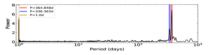
Figure 11: GLS periodogram of our observation sampling window function. The three prominent periods are shown using thick coloured lines with their respective values listed in the plot legend. The x-axis is shown in logarithmic scale.

Table 3: Observation log of the GJ 436 system observed by the NARVAL spectropolarimeter in 2016. The table contains the Signal-to-Noise ratio (SNR) and the H$\alpha$, NaI, CaII H&K, CaI, HeI and CaII IRT activity indices along with their errors. The total exposure time for each observation spectra is 4$\times$700s.

Date (2016)	HJD (2457000+)	UT (h:m:s)	S/N	H$\alpha$	NaI	CaI	CaII H	HeI	IRT1	IRT2	IRT3
Mar 16	464.49670	23:49:19	203	0.4109 ± 0.0010	0.2144 ± 0.0022	0.3346 ± 0.0012	1.2210 ± 0.0960	0.4677 ± 0.0041	0.3021 ± 0.0007	0.2323 ± 0.0008	0.2156 ± 0.0006
Mar 18	465.52978	00:36:58	204	0.4101 ± 0.0010	0.2300 ± 0.0022	0.3354 ± 0.0011	1.0388 ± 0.0927	0.4867 ± 0.0041	0.3083 ± 0.0007	0.2329 ± 0.0008	0.2158 ± 0.0006
Mar 20	468.47996	23:25:14	274	0.4096 ± 0.0007	0.2159 ± 0.0013	0.3326 ± 0.0008	1.1705 ± 0.0499	0.4799 ± 0.0026	0.3032 ± 0.0005	0.2387 ± 0.0006	0.2171 ± 0.0004
Apr 18	497.40198	21:33:54	235	0.4102 ± 0.0008	0.2148 ± 0.0016	0.3385 ± 0.0009	1.1727 ± 0.0573	0.4791 ± 0.0032	0.3036 ± 0.0006	0.2465 ± 0.0007	0.2167 ± 0.0004
May 02	511.46867	23:10:51	275	0.4145 ± 0.0007	0.2110 ± 0.0013	0.3335 ± 0.0008	1.1942 ± 0.0444	0.4750 ± 0.0026	0.3068 ± 0.0005	0.2391 ± 0.0006	0.2163 ± 0.0004
May 03	512.48383	23:32:45	227	0.4102 ± 0.0009	0.2176 ± 0.0018	0.3382 ± 0.0010	1.0720 ± 0.0650	0.4774 ± 0.0034	0.3061 ± 0.0006	0.2376 ± 0.0007	0.2165 ± 0.0005
May 04	513.39868	21:30:12	234	0.4061 ± 0.0008	0.2141 ± 0.0017	0.3340 ± 0.0010	1.1243 ± 0.0631	0.4725 ± 0.0033	0.3068 ± 0.0006	0.2381 ± 0.0007	0.2169 ± 0.0004
May 11	520.35975	20:34:43	204	0.4100 ± 0.0010	0.2051 ± 0.0020	0.3346 ± 0.0011	1.1530 ± 0.0763	0.4846 ± 0.0039	0.3026 ± 0.0007	0.2283 ± 0.0008	0.2224 ± 0.0005
May 16	525.36718	20:45:50	273	0.4080 ± 0.0007	0.2122 ± 0.0013	0.3325 ± 0.0008	1.2993 ± 0.0458	0.4795 ± 0.0026	0.3031 ± 0.0005	0.2315 ± 0.0006	0.2216 ± 0.0004
May 17	526.36784	20:46:53	216	0.4073 ± 0.0009	0.2212 ± 0.0018	0.3338 ± 0.0010	0.9972 ± 0.0617	0.4774 ± 0.0034	0.3031 ± 0.0007	0.2308 ± 0.0007	0.2230 ± 0.0005
May 20	529.38615	21:13:31	219	0.4078 ± 0.0009	0.2093 ± 0.0019	0.3334 ± 0.0011	1.1308 ± 0.0752	0.4756 ± 0.0036	0.3072 ± 0.0006	0.2352 ± 0.0007	0.2206 ± 0.0005
May 23	532.37271	20:54:26	233	0.4092 ± 0.0008	0.2069 ± 0.0017	0.3322 ± 0.0010	1.1895 ± 0.0653	0.4821 ± 0.0032	0.3057 ± 0.0006	0.2382 ± 0.0007	0.2156 ± 0.0005
Jun 02	542.37484	20:58:28	219	0.4047 ± 0.0009	0.2192 ± 0.0019	0.3331 ± 0.0010	1.1213 ± 0.0690	0.4765 ± 0.0035	0.3051 ± 0.0006	0.2329 ± 0.0007	0.2206 ± 0.0005
Jun 04	544.38322	21:10:44	212	0.4090 ± 0.0009	0.2100 ± 0.0019	0.3287 ± 0.0011	1.0549 ± 0.0731	0.4819 ± 0.0037	0.3075 ± 0.0007	0.2303 ± 0.0007	0.2245 ± 0.0005
Jun 07	547.37509	20:59:19	272	0.4045 ± 0.0007	0.2060 ± 0.0013	0.3412 ± 0.0008	1.3019 ± 0.0517	0.4744 ± 0.0027	0.3078 ± 0.0005	0.2387 ± 0.0006	0.2227 ± 0.0004
Jun 08	548.37866	21:04:34	289	0.4042 ± 0.0007	0.2058 ± 0.0012	0.3326 ± 0.0008	1.2250 ± 0.0410	0.4756 ± 0.0025	0.3064 ± 0.0005	0.2332 ± 0.0006	0.2218 ± 0.0003

Table 4: Observation log of the GJ 436 system observed by HARPS from 2006 to 2020. The table contains the total exposure time $t_{exp}$ (s), median Signal-to-Noise ratio (SNR) and the H$\alpha$, NaI, CaII H&K, CaI and HeI activity indices along with their errors

Date	BJD (2450000+)	UT (h:m:s)	$t_{exp}$(s)	S/N	H$\alpha$	NaI	CaII	CaI	HeI
2006-01-25	3760.835	07:49:14.289	900.0017	22.25	0.4074±0.0008	0.1803±0.0016	0.5040±0.0166	0.3381±0.0011	0.4845±0.0028
2006-01-26	3761.840	07:55:59.746	900.0012	21.85	0.4133±0.0008	0.1758±0.0015	0.6016±0.0180	0.3404±0.0011	0.4822±0.0028
2006-01-27	3762.827	07:37:50.432	900.0006	31.55	0.4118±0.0006	0.1775±0.0011	0.5990±0.0102	0.3400±0.0008	0.4733±0.0020
2006-01-28	3763.841	07:57:34.268	900.0005	31.70	0.4143±0.0006	0.1765±0.0011	0.5542±0.0099	0.3420±0.0008	0.4775±0.0020
2006-01-30	3765.803	07:02:58.125	900.0012	28.60	0.4110±0.0007	0.1738±0.0012	0.5730±0.0117	0.3430±0.0008	0.4765±0.0022
2006-02-19	3785.760	05:59:45.661	900.0025	29.40	0.4102±0.0006	0.1823±0.0012	0.5527±0.0107	0.3422±0.0008	0.4802±0.0022
2006-02-22	3788.779	06:26:37.814	900.0009	32.15	0.4083±0.0006	0.1827±0.0011	0.5920±0.0092	0.3393±0.0008	0.4806±0.0020
2007-01-22	4122.842	07:59:34.392	900.0001	30.70	0.4139±0.0006	0.1797±0.0011	0.5892±0.0094	0.3382±0.0008	0.4837±0.0020
2007-02-04	4135.832	07:43:32.169	900.0017	31.05	0.4055±0.0006	0.1818±0.0011	0.5882±0.0091	0.3385±0.0008	0.4794±0.0021
2007-02-09	4140.821	07:27:50.165	900.0034	24.65	0.4122±0.0008	0.1858±0.0014	0.5660±0.0123	0.3374±0.0010	0.4807±0.0025
2007-02-11	4142.830	07:39:59.325	900.0021	30.40	0.4106±0.0006	0.1842±0.0011	0.6034±0.0095	0.3383±0.0008	0.4812±0.0020
2007-03-07	4166.750	05:44:40.764	899.9954	20.50	0.4116±0.0009	0.1847±0.0017	0.5995±0.0168	0.3408±0.0011	0.4883±0.0029
2007-03-13	4172.742	05:33:24.847	899.9972	25.75	0.4102±0.0007	0.1831±0.0013	0.5836±0.0120	0.3402±0.0009	0.4904±0.0024
2007-04-04	4194.708	04:45:48.825	899.9961	18.00	0.4138±0.0010	0.1923±0.0019	0.6751±0.0194	0.3374±0.0012	0.4828±0.0032
2007-04-07	4197.677	04:00:25.671	900.0021	21.60	0.4144±0.0008	0.1860±0.0015	0.6153±0.0153	0.3403±0.0010	0.4759±0.0027
2007-04-09	4199.670	03:51:11.405	900.0019	26.95	0.4114±0.0007	0.1568±0.0011	0.5768±0.0113	0.3362±0.0009	0.4814±0.0023
2007-04-12	4202.663	03:41:50.693	899.9963	27.90	0.4204±0.0007	0.1863±0.0012	0.6834±0.0108	0.3376±0.0008	0.4832±0.0022
2007-05-08	4228.582	01:47:05.634	899.9962	23.95	0.4095±0.0007	0.1805±0.0014	0.6053±0.0124	0.3370±0.0010	0.4789±0.0025
2007-05-09	4230.485	23:27:20.751	899.9945	19.60	0.4113±0.0009	0.1831±0.0016	0.6404±0.0171	0.3352±0.0011	0.4795±0.0030
2007-05-09	4230.494	23:43:27.584	599.9964	17.10	0.4128±0.0010	0.1846±0.0019	0.6366±0.0196	0.3360±0.0013	0.4771±0.0033
2007-05-09	4230.501	23:54:54.201	300.0005	10.70	0.4106±0.0015	0.1759±0.0028	0.8489±0.0374	0.3409±0.0019	0.4755±0.0049
2007-05-10	4230.504	00:00:25.159	300.0005	11.10	0.4099±0.0014	0.1752±0.0027	0.5973±0.0341	0.3388±0.0018	0.4762±0.0048
2007-05-10	4230.508	00:05:55.997	300.0026	12.40	0.4077±0.0013	0.1779±0.0025	0.5534±0.0295	0.3348±0.0017	0.4783±0.0043
2007-05-10	4230.512	00:11:26.685	300.0052	13.10	0.4087±0.0012	0.1749±0.0023	0.5295±0.0278	0.3367±0.0016	0.4815±0.0041
2007-05-10	4230.516	00:16:57.222	300.0005	11.60	0.4140±0.0014	0.1782±0.0026	0.5631±0.0328	0.3386±0.0018	0.4820±0.0046
2007-05-10	4230.520	00:22:28.100	300.0007	11.80	0.4119±0.0014	0.1727±0.0025	0.6076±0.0312	0.3365±0.0018	0.4768±0.0046
2007-05-10	4230.524	00:27:58.888	300.0001	6.95	0.4122±0.0021	0.1605±0.0040	0.6579±0.0577	0.3399±0.0028	0.4845±0.0070
2007-05-10	4230.527	00:33:29.836	299.9996	9.60	0.4098±0.0016	0.1687±0.0030	0.5521±0.0393	0.3419±0.0021	0.4770±0.0054
2007-05-10	4230.531	00:39:00.604	300.0049	11.80	0.4084±0.0014	0.1733±0.0026	0.7377±0.0319	0.3393±0.0018	0.4752±0.0046
2007-05-10	4230.535	00:44:31.482	299.9988	13.55	0.4119±0.0012	0.1817±0.0024	0.6330±0.0256	0.3355±0.0016	0.4759±0.0041
2007-05-10	4230.539	00:50:02.370	300.0036	13.90	0.4121±0.0012	0.1800±0.0023	0.6145±0.0249	0.3391±0.0016	0.4796±0.0040
2007-05-10	4230.543	00:55:33.418	300.0006	14.05	0.4117±0.0012	0.1785±0.0023	0.6778±0.0251	0.3409±0.0016	0.4862±0.0040
2007-05-10	4230.546	01:01:04.366	300.0007	13.90	0.4093±0.0012	0.1784±0.0023	0.6504±0.0260	0.3382±0.0016	0.4802±0.0041
2007-05-10	4230.550	01:06:35.533	300.0032	14.00	0.4097±0.0012	0.1786±0.0022	0.6397±0.0253	0.3411±0.0016	0.4785±0.0040
2007-05-10	4230.554	01:12:06.511	299.9994	13.75	0.4135±0.0012	0.1802±0.0023	0.6856±0.0269	0.3373±0.0016	0.4918±0.0042
2007-05-10	4230.558	01:17:37.779	299.9975	15.25	0.4121±0.0011	0.1774±0.0021	0.6274±0.0228	0.3390±0.0014	0.4756±0.0037
2007-05-10	4230.562	01:23:08.497	299.9991	15.80	0.4095±0.0011	0.1764±0.0020	0.7011±0.0224	0.3394±0.0014	0.4772±0.0036
2007-05-10	4230.566	01:28:39.555	300.0008	14.70	0.4103±0.0012	0.1830±0.0022	0.6819±0.0238	0.3382±0.0015	0.4789±0.0038
2007-05-10	4230.569	01:34:10.553	300.0056	14.65	0.4163±0.0012	0.1847±0.0022	0.6955±0.0238	0.3405±0.0015	0.4831±0.0039
2007-05-10	4230.573	01:39:41.541	300.0054	17.45	0.4174±0.0010	0.1858±0.0019	0.7150±0.0191	0.3389±0.0013	0.4776±0.0033
2007-05-10	4230.577	01:45:12.469	300.0042	17.10	0.4159±0.0010	0.1827±0.0019	0.7362±0.0204	0.3386±0.0013	0.4704±0.0033
2007-05-10	4230.581	01:50:43.807	300.0002	14.35	0.4100±0.0012	0.1815±0.0022	0.7038±0.0245	0.3372±0.0015	0.4817±0.0039
2007-05-10	4230.585	01:56:14.615	299.9981	16.95	0.4092±0.0010	0.1880±0.0020	0.6465±0.0196	0.3384±0.0013	0.4827±0.0035
2007-05-10	4230.589	02:01:45.983	299.9997	17.05	0.4099±0.0010	0.1788±0.0019	0.6350±0.0193	0.3397±0.0013	0.4759±0.0034
2007-05-10	4230.592	02:07:17.221	299.9982	14.80	0.4139±0.0012	0.1768±0.0021	0.5695±0.0230	0.3388±0.0015	0.4798±0.0038
2007-05-10	4230.596	02:12:48.108	299.9979	15.70	0.4099±0.0011	0.1787±0.0020	0.5888±0.0209	0.3380±0.0014	0.4792±0.0037
2007-05-10	4230.600	02:18:18.966	300.0016	12.70	0.409±0.00130	0.1722±0.0024	0.6108±0.0280	0.3378±0.0017	0.4764±0.0044
2007-05-10	4230.604	02:23:49.754	300.0013	13.25	0.4077±0.0013	0.1810±0.0024	0.5406±0.0258	0.3372±0.0016	0.4809±0.0042
2007-05-10	4230.608	02:29:20.712	299.9999	11.30	0.4066±0.0014	0.1747±0.0027	0.6489±0.0331	0.3374±0.0019	0.4798±0.0048
2007-05-10	4230.612	02:34:51.480	299.9953	11.05	0.4113±0.0014	0.1775±0.0028	0.5282±0.0343	0.3366±0.0019	0.4819±0.0049

2007-05-10	4230.615	02:40:22.158	300.0006	9.60	0.4137±0.0016	0.1723±0.0031	0.6209±0.0405	0.3361±0.0021	0.4799±0.0055
2007-05-10	4230.619	02:45:52.966	299.9987	9.95	0.4147±0.0016	0.1700±0.0030	0.6503±0.0409	0.3402±0.0021	0.4810±0.0053
2007-05-10	4230.623	02:51:23.774	299.9947	10.25	0.412±0.00160	0.1721±0.0029	0.6887±0.0381	0.3397±0.0020	0.4854±0.0052
2007-05-10	4230.627	02:56:54.752	299.9947	13.45	0.4125±0.0012	0.1826±0.0024	0.6512±0.0274	0.3382±0.0016	0.4727±0.0041
2007-05-10	4230.631	03:02:25.609	299.9954	14.00	0.4083±0.0012	0.1783±0.0022	0.6801±0.0260	0.3368±0.0015	0.4833±0.0040
2007-05-10	4230.635	03:07:56.437	299.9947	15.95	0.4125±0.0011	0.1807±0.0020	0.6487±0.0226	0.3371±0.0014	0.4809±0.0036
2007-05-10	4230.639	03:13:53.497	299.9947	15.75	0.4119±0.0011	0.1799±0.0020	0.6100±0.0226	0.3370±0.0014	0.4799±0.0036
2007-05-10	4230.643	03:19:24.165	299.9956	16.40	0.4097±0.0011	0.1780±0.0019	0.6151±0.0212	0.3376±0.0013	0.4763±0.0034
2007-05-10	4230.646	03:24:55.132	299.9995	15.95	0.4089±0.0011	0.1800±0.0020	0.5529±0.0214	0.3379±0.0014	0.4825±0.0036
2007-05-10	4230.650	03:30:26.120	299.9947	16.55	0.4106±0.0010	0.1754±0.0019	0.5685±0.0210	0.3356±0.0013	0.4761±0.0034
2007-05-10	4230.654	03:35:57.118	299.9945	15.60	0.4075±0.0011	0.1808±0.0020	0.5998±0.0235	0.3370±0.0014	0.4765±0.0035
2007-05-10	4230.658	03:41:28.076	299.9956	14.60	0.4119±0.0011	0.1832±0.0021	0.7136±0.0269	0.3395±0.0014	0.4776±0.0036
2007-05-14	4234.553	01:05:12.938	899.9974	19.55	0.4142±0.0009	0.1843±0.0017	0.6804±0.0176	0.3406±0.0011	0.4825±0.0030
2007-06-02	4253.545	00:49:00.762	1799.9950	22.75	0.4089±0.0008	0.1838±0.0015	0.5051±0.0139	0.3389±0.0010	0.4793±0.0026
2007-06-03	4254.511	00:01:11.437	1799.9976	19.45	0.4073±0.0009	0.1617±0.0015	0.5947±0.0181	0.3380±0.0012	0.4766±0.0030
2007-06-04	4255.516	00:01:55.802	1999.9987	20.15	0.4074±0.0009	0.1806±0.0016	0.5530±0.0169	0.3387±0.0011	0.4733±0.0029
2007-06-07	4259.487	23:25:53.536	1800.0005	33.95	0.4077±0.0005	0.1766±0.0010	0.5268±0.0077	0.3392±0.0007	0.4814±0.0018
2007-07-09	4291.488	23:39:41.130	899.9997	10.85	0.4150±0.0014	0.1745±0.0027	0.6260±0.0534	0.3380±0.0018	0.4762±0.0048
2007-07-10	4292.474	23:19:57.798	899.9983	27.65	0.4099±0.0007	0.1818±0.0012	0.6225±0.0109	0.3362±0.0009	0.4755±0.0022
2007-07-11	4293.451	22:46:11.010	899.9988	34.25	0.4126±0.0005	0.1841±0.0010	0.6210±0.0082	0.3387±0.0007	0.4791±0.0017
2007-07-12	4294.449	22:44:03.574	900.0002	23.85	0.4089±0.0007	0.1852±0.0014	0.5741±0.0123	0.3381±0.0009	0.4713±0.0024
2007-07-14	4296.476	23:23:09.149	900.0002	16.35	0.4062±0.0010	0.1838±0.0019	0.6394±0.0226	0.3399±0.0013	0.4777±0.0034
2007-07-15	4297.453	22:49:24.843	899.9997	26.00	0.4082±0.0007	0.1817±0.0012	0.5832±0.0111	0.3393±0.0009	0.4794±0.0023
2008-01-13	4478.852	08:14:31.312	900.0000	27.70	0.4170±0.0007	0.1755±0.0012	0.5035±0.0097	0.3357±0.0008	0.4802±0.0022
2008-01-13	4478.878	08:51:43.283	900.0000	28.50	0.4175±0.0007	0.1790±0.0012	0.5493±0.0095	0.3364±0.0008	0.4786±0.0021
2008-01-14	4479.865	08:32:55.089	900.0000	23.35	0.4171±0.0008	0.1777±0.0014	0.5532±0.0127	0.3348±0.0010	0.4808±0.0026
2008-01-14	4479.875	08:48:25.929	900.0000	24.75	0.4168±0.0008	0.1792±0.0013	0.5319±0.0115	0.3353±0.0009	0.4864±0.0025
2008-01-15	4480.858	08:24:14.411	900.0000	26.85	0.4166±0.0007	0.1748±0.0012	0.5144±0.0103	0.3347±0.0009	0.4832±0.0023
2008-01-15	4480.870	08:39:45.762	900.0000	22.20	0.4157±0.0008	0.1719±0.0014	0.5377±0.0134	0.3336±0.0010	0.4783±0.0027
2008-01-16	4481.862	08:29:09.201	900.0000	26.80	0.4190±0.0007	0.1663±0.0012	0.5672±0.0106	0.3359±0.0009	0.4746±0.0023
2008-01-16	4481.873	08:44:40.662	900.0000	28.55	0.4188±0.0007	0.1732±0.0011	0.5863±0.0098	0.3351±0.0008	0.4736±0.0021
2008-01-17	4482.853	08:15:59.848	900.0000	23.45	0.4161±0.0008	0.1637±0.0013	0.5629±0.0123	0.3364±0.0010	0.4768±0.0026
2008-01-17	4482.864	08:31:30.948	900.0000	23.80	0.4167±0.0008	0.1712±0.0013	0.5668±0.0122	0.3340±0.0010	0.4718±0.0025
2008-01-18	4483.852	08:13:36.738	900.0000	25.30	0.4202±0.0007	0.1742±0.0013	0.5877±0.0117	0.3364±0.0009	0.4761±0.0024
2008-01-18	4483.863	08:29:08.038	900.0000	28.15	0.4217±0.0007	0.1743±0.0011	0.5809±0.0101	0.3355±0.0008	0.4775±0.0021
2008-01-20	4485.857	08:20:53.267	900.0000	25.40	0.4193±0.0007	0.1795±0.0013	0.5849±0.0118	0.3362±0.0009	0.4820±0.0024
2008-01-20	4485.868	08:36:24.928	900.0000	25.50	0.4160±0.0007	0.1775±0.0013	0.5293±0.0116	0.3378±0.0009	0.4788±0.0024
2008-01-21	4486.854	08:16:30.074	900.0000	23.40	0.4156±0.0008	0.1786±0.0014	0.5554±0.0131	0.3366±0.0010	0.4776±0.0026
2008-01-21	4486.864	08:32:01.905	900.0000	21.10	0.4144±0.0009	0.1798±0.0016	0.5586±0.0153	0.3368±0.0011	0.4793±0.0028
2008-01-22	4487.851	08:12:19.811	900.0000	18.95	0.4125±0.0009	0.1749±0.0017	0.4912±0.0167	0.3377±0.0012	0.4790±0.0031
2008-01-22	4487.862	08:27:53.061	900.0000	23.30	0.4146±0.0008	0.1756±0.0014	0.5229±0.0128	0.3409±0.0010	0.4802±0.0026
2008-01-23	4488.854	08:17:27.757	900.0000	21.65	0.4176±0.0008	0.1818±0.0015	0.5368±0.0141	0.3390±0.0011	0.4762±0.0027
2008-02-26	4522.838	07:51:57.296	900.0000	17.80	0.4101±0.0009	0.1833±0.0018	0.6189±0.0192	0.3414±0.0012	0.4767±0.0031
2008-02-27	4523.789	06:40:48.149	900.0000	22.90	0.4196±0.0008	0.1823±0.0014	0.6434±0.0129	0.3405±0.0010	0.4911±0.0026
2008-02-28	4524.789	06:41:55.545	900.0000	31.30	0.4085±0.0006	0.1782±0.0011	0.5228±0.0082	0.3381±0.0008	0.4791±0.0020
2008-02-29	4525.812	07:15:20.355	900.0000	21.20	0.4098±0.0008	0.1745±0.0015	0.5269±0.0143	0.3398±0.0011	0.4793±0.0027
2008-03-01	4526.763	06:03:17.367	900.0000	30.85	0.4119±0.0006	0.1761±0.0011	0.5449±0.0085	0.3391±0.0008	0.4806±0.0020
2008-03-02	4527.751	05:46:18.300	900.0000	26.60	0.4135±0.0007	0.1749±0.0012	0.5139±0.0103	0.3384±0.0009	0.4825±0.0022
2008-03-03	4528.717	04:56:50.095	900.0000	28.75	0.4171±0.0006	0.1669±0.0010	0.6229±0.0096	0.3402±0.0008	0.4821±0.0021
2008-03-04	4529.812	07:13:47.000	900.0000	25.40	0.4157±0.0007	0.1759±0.0012	0.5258±0.0113	0.3411±0.0009	0.4846±0.0023
2008-03-05	4530.777	06:23:27.951	900.0000	26.35	0.4131±0.0007	0.1765±0.0012	0.5471±0.0107	0.3422±0.0009	0.4823±0.0022
2008-03-23	4548.703	04:29:09.320	1800.0000	31.95	0.4120±0.0006	0.1832±0.0010	0.6551±0.0086	0.3374±0.0007	0.4805±0.0019
2008-03-24	4549.697	04:23:08.332	1800.0000	20.80	0.4070±0.0009	0.1870±0.0016	0.5574±0.0142	0.3351±0.0011	0.4801±0.0029
2008-03-26	4551.718	04:50:59.515	1800.0000	27.15	0.4134±0.0007	0.1816±0.0012	0.6116±0.0106	0.3387±0.0008	0.4783±0.0022
2008-03-28	4553.697	04:20:30.367	1800.0000	39.50	0.4098±0.0005	0.1779±0.0008	0.5803±0.0064	0.3392±0.0006	0.4839±0.0015
2008-04-01	4557.658	03:31:59.932	900.0000	21.30	0.4120±0.0008	0.1820±0.0015	0.5680±0.0154	0.3381±0.0011	0.4825±0.0027
2008-04-06	4562.644	03:13:07.077	900.0000	25.55	0.4191±0.0007	0.1848±0.0013	0.6829±0.0111	0.3393±0.0009	0.4775±0.0023
2008-04-08	4564.647	03:17:17.360	900.0000	18.40	0.4067±0.0009	0.1794±0.0017	0.5865±0.0166	0.3390±0.0012	0.4770±0.0031
2008-04-11	4567.565	01:18:00.524	1200.0000	36.80	0.4135±0.0005	0.1801±0.0009	0.5887±0.0068	0.3370±0.0006	0.4823±0.0016
2008-04-11	4567.734	05:21:29.227	1200.0000	31.85	0.4106±0.0005	0.1748±0.0010	0.5584±0.0088	0.3377±0.0007	0.4822±0.0018
2008-04-12	4568.570	01:24:47.042	1200.0000	31.00	0.4121±0.0006	0.1811±0.0010	0.5568±0.0084	0.3381±0.0007	0.4826±0.0019
2008-04-12	4568.691	04:18:39.251	1200.0000	27.65	0.4113±0.0007	0.1771±0.0011	0.5483±0.0099	0.3377±0.0008	0.4839±0.0021
2008-04-13	4569.628	02:48:27.256	1200.0000	33.00	0.4115±0.0006	0.1764±0.0010	0.5453±0.0076	0.3371±0.0007	0.4818±0.0018
2008-04-14	4570.637	03:01:26.706	1200.0000	29.00	0.4100±0.0006	0.1744±0.0011	0.5710±0.0092	0.3368±0.0008	0.4843±0.0021
2008-04-15	4571.609	02:20:57.077	1200.0000	24.30	0.4100±0.0007	0.1817±0.0013	0.6037±0.0116	0.3367±0.0009	0.4827±0.0024
2008-05-07	4593.551	01:02:54.710	900.0000	27.20	0.4097±0.0007	0.1800±0.0012	0.5546±0.0107	0.3366±0.0009	0.4840±0.0022
2008-05-23	4610.478	23:20:22.079	900.0000	21.15	0.4089±0.0008	0.1771±0.0015	0.5964±0.0162	0.3379±0.0011	0.4791±0.0028
2008-05-24	4610.562	01:21:06.631	900.0000	22.25	0.4077±0.0008	0.1779±0.0014	0.5571±0.0149	0.3387±0.0010	0.4753±0.0026
2008-05-25	4611.557	01:13:01.347	900.0000	24.10	0.4074±0.0007	0.1773±0.0013	0.5630±0.0130	0.3370±0.0010	0.4834±0.0025

2008-05-29	4616.476	23:17:49.454	900.0000	15.40	0.4099±0.0011	0.1759±0.0020	0.5896±0.0243	0.3339±0.0014	0.4764±0.0037
2009-01-01	4832.876	08:50:43.355	900.0000	19.75	0.4099±0.0009	0.1875±0.0017	0.4952±0.0138	0.3357±0.0012	0.4773±0.0030
2009-01-17	4848.871	08:40:56.016	900.0000	24.90	0.4116±0.0008	0.1791±0.0013	0.5695±0.0113	0.3368±0.0010	0.4752±0.0025
2009-01-23	4854.846	08:05:36.145	900.0000	23.60	0.4147±0.0008	0.1821±0.0014	0.6078±0.0126	0.3386±0.0010	0.4806±0.0025
2009-02-16	4878.789	06:41:42.107	900.0000	28.35	0.4130±0.0007	0.1764±0.0011	0.4927±0.0098	0.3409±0.0008	0.4783±0.0021
2009-02-17	4879.791	06:44:41.282	900.0000	15.40	0.4117±0.0011	0.1775±0.0020	0.5336±0.0260	0.3406±0.0014	0.4819±0.0036
2009-02-18	4880.797	06:53:32.974	900.0000	11.95	0.4151±0.0014	0.1770±0.0026	0.7077±0.0368	0.3396±0.0018	0.4942±0.0046
2009-02-18	4880.812	07:14:56.353	900.0000	18.45	0.4172±0.0010	0.1768±0.0017	0.5535±0.0186	0.3410±0.0013	0.4861±0.0032
2009-02-19	4881.787	06:38:37.801	900.0000	25.60	0.4140±0.0007	0.1766±0.0013	0.5375±0.0117	0.3413±0.0009	0.4821±0.0023
2009-02-20	4882.784	06:33:25.497	900.0000	21.45	0.4123±0.0008	0.1767±0.0015	0.4987±0.0149	0.3405±0.0011	0.4764±0.0027
2009-02-21	4883.794	06:48:10.721	900.0000	28.80	0.4126±0.0006	0.1784±0.0011	0.5113±0.0095	0.3395±0.0008	0.4819±0.0021
2009-02-22	4884.773	06:18:11.456	900.0000	15.90	0.4107±0.0011	0.1769±0.0020	0.5065±0.0201	0.3376±0.0015	0.4825±0.0037
2009-02-23	4885.792	06:45:47.206	900.0000	29.85	0.4126±0.0006	0.1792±0.0011	0.5290±0.0086	0.3379±0.0008	0.4788±0.0020
2009-02-24	4886.769	06:12:47.455	900.0000	21.65	0.4114±0.0008	0.1772±0.0014	0.5510±0.0132	0.3405±0.0010	0.4902±0.0026
2009-03-23	4913.688	04:15:54.065	900.0000	27.95	0.4063±0.0006	0.1812±0.0012	0.5356±0.0094	0.3372±0.0008	0.4717±0.0021
2009-03-24	4914.708	04:44:20.901	900.0000	24.75	0.4059±0.0007	0.1812±0.0013	0.5933±0.0117	0.3377±0.0009	0.4783±0.0023
2009-03-25	4915.687	04:14:59.071	900.0000	22.95	0.4065±0.0008	0.1801±0.0014	0.5389±0.0125	0.3384±0.0010	0.4740±0.0025
2009-03-26	4916.692	04:22:10.575	900.0000	27.05	0.4052±0.0007	0.1764±0.0012	0.5701±0.0101	0.3387±0.0008	0.4727±0.0022
2009-03-27	4917.680	04:04:13.404	900.0000	24.20	0.4087±0.0007	0.1802±0.0013	0.5709±0.0116	0.3391±0.0009	0.4757±0.0024
2009-03-28	4918.727	05:12:44.335	900.0000	25.25	0.4091±0.0007	0.1781±0.0013	0.5841±0.0111	0.3369±0.0009	0.4760±0.0023
2009-03-29	4919.662	03:39:11.570	900.0000	23.75	0.4121±0.0007	0.1820±0.0013	0.5875±0.0118	0.3390±0.0009	0.4800±0.0024
2009-03-30	4920.707	04:43:16.572	900.0000	26.70	0.4111±0.0007	0.1821±0.0012	0.5583±0.0101	0.3380±0.0009	0.4793±0.0022
2009-04-11	4932.643	03:11:18.807	900.0000	16.65	0.4095±0.0010	0.1811±0.0019	0.5416±0.0175	0.3371±0.0013	0.4872±0.0034
2009-04-12	4933.638	03:04:47.794	900.0000	22.30	0.4077±0.0008	0.1775±0.0014	0.5602±0.0122	0.3392±0.0010	0.4748±0.0026
2009-04-13	4934.626	02:47:59.458	900.0000	24.25	0.4079±0.0007	0.1688±0.0012	0.5700±0.0112	0.3384±0.0009	0.4792±0.0024
2009-04-15	4936.632	02:56:56.447	900.0000	14.20	0.4051±0.0012	0.1763±0.0022	0.5988±0.0193	0.3413±0.0016	0.4771±0.0039
2009-04-16	4937.611	02:27:03.710	900.0000	18.95	0.4081±0.0009	0.1816±0.0017	0.5524±0.0153	0.3375±0.0012	0.4771±0.0030
2009-04-17	4938.623	02:43:32.285	900.0000	27.10	0.4064±0.0007	0.1797±0.0012	0.5556±0.0095	0.3384±0.0008	0.4768±0.0022
2009-04-18	4939.639	03:06:34.539	900.0000	14.70	0.4085±0.0011	0.1785±0.0021	0.6309±0.0216	0.3366±0.0015	0.4789±0.0037
2009-04-19	4940.614	02:31:35.787	900.0000	15.45	0.4071±0.0011	0.1822±0.0020	0.6253±0.0203	0.3364±0.0014	0.4722±0.0035
2009-04-20	4941.622	02:43:00.570	900.0000	25.80	0.4031±0.0007	0.1781±0.0012	0.5901±0.0102	0.3360±0.0009	0.4796±0.0023
2009-04-25	4946.604	02:17:43.389	900.0000	30.90	0.4074±0.0006	0.1799±0.0011	0.5507±0.0079	0.3377±0.0008	0.4793±0.0019
2009-04-28	4949.582	01:46:07.435	900.0000	26.10	0.4056±0.0007	0.1821±0.0013	0.5672±0.0100	0.3378±0.0009	0.4714±0.0023
2009-04-29	4950.583	01:47:55.171	900.0000	27.85	0.4082±0.0007	0.1830±0.0012	0.5761±0.0093	0.3358±0.0008	0.4769±0.0021
2009-05-02	4953.588	01:54:52.741	900.0000	23.20	0.4035±0.0008	0.1594±0.0012	0.5286±0.0128	0.3375±0.0010	0.4780±0.0025
2009-05-03	4954.583	01:47:54.873	900.0000	26.75	0.4042±0.0007	0.1640±0.0011	0.5361±0.0104	0.3399±0.0009	0.4750±0.0022
2009-05-04	4955.582	01:45:25.155	900.0000	26.00	0.3985±0.0007	0.1766±0.0012	0.5283±0.0107	0.3384±0.0009	0.4761±0.0023
2009-05-05	4956.583	01:48:12.726	900.0000	18.65	0.3962±0.0009	0.1787±0.0017	0.5301±0.0176	0.3385±0.0012	0.4691±0.0030
2009-06-07	4990.498	23:49:42.435	899.9994	20.80	0.4063±0.0008	0.1812±0.0015	0.4462±0.0145	0.3373±0.0011	0.4814±0.0027
2009-06-09	4991.510	00:07:46.413	900.0005	24.70	0.4061±0.0008	0.1817±0.0013	0.4472±0.0111	0.3375±0.0010	0.4828±0.0024
2009-06-10	4993.465	23:02:22.549	899.9991	26.40	0.4060±0.0007	0.1807±0.0012	0.5055±0.0104	0.3369±0.0009	0.4779±0.0022
2010-03-17	5272.702	04:35:49.928	899.9998	21.05	0.4093±0.0008	0.1778±0.0015	0.4912±0.0149	0.3386±0.0011	0.4769±0.0027
2010-03-20	5275.707	04:43:15.807	900.0068	16.30	0.4089±0.0010	0.1820±0.0019	0.5149±0.0227	0.3399±0.0013	0.4734±0.0033
2010-03-22	5277.711	04:48:38.792	899.9990	16.30	0.4173±0.0010	0.1808±0.0018	0.7036±0.0223	0.3392±0.0012	0.4816±0.0032
2010-03-23	5278.703	04:36:33.665	899.9985	11.65	0.4085±0.0014	0.1752±0.0025	0.4999±0.0365	0.3368±0.0018	0.4836±0.0045
2010-03-24	5279.684	04:09:33.598	899.9987	19.40	0.4083±0.0009	0.1815±0.0016	0.4946±0.0171	0.3376±0.0012	0.4757±0.0029
2010-03-25	5280.700	04:33:03.332	900.0001	19.20	0.4097±0.0009	0.1807±0.0017	0.4938±0.0170	0.3370±0.0012	0.4760±0.0030
2010-03-28	5283.677	04:00:55.642	900.0064	26.35	0.4120±0.0007	0.1792±0.0012	0.5204±0.0095	0.3387±0.0009	0.4828±0.0022
2010-04-01	5287.655	03:29:21.475	899.9999	21.65	0.4096±0.0008	0.1856±0.0015	0.5895±0.0131	0.3363±0.0010	0.4778±0.0026
2010-04-06	5292.649	03:22:20.916	900.0069	8.00	0.4046±0.0018	0.1870±0.0037	0.4311±0.0376	0.3381±0.0024	0.4704±0.0059
2020-01-28	8876.843	08:00:12.543	899.9976	25.05	0.4169±0.0007	0.1909±0.0012	0.5824±0.0096	0.3384±0.0009	0.4783±0.0022
2020-01-31	8879.843	07:59:54.501	899.9977	17.35	0.4131±0.0009	0.1914±0.0017	0.6253±0.0140	0.3387±0.0012	0.4778±0.0029
2020-02-01	8880.832	07:44:08.123	899.9977	20.30	0.4083±0.0008	0.1855±0.0014	0.6500±0.0123	0.3392±0.0010	0.4852±0.0026
2020-02-02	8881.852	08:12:40.567	899.9977	20.95	0.4090±0.0008	0.1913±0.0014	0.5655±0.0116	0.3391±0.0010	0.4733±0.0024
2020-02-03	8882.828	07:38:09.453	899.9978	21.95	0.4134±0.0008	0.1923±0.0014	0.6192±0.0112	0.3377±0.0010	0.4814±0.0024
2020-02-04	8883.812	07:14:14.400	899.9978	20.70	0.4159±0.0008	0.1917±0.0014	0.5734±0.0115	0.3385±0.0010	0.4805±0.0026
2020-02-05	8884.804	07:02:56.565	899.9977	17.75	0.4136±0.0010	0.1933±0.0017	0.5235±0.0120	0.3374±0.0012	0.4788±0.0030
2020-02-07	8886.797	06:53:35.306	899.9977	21.15	0.4144±0.0008	0.1971±0.0015	0.6101±0.0110	0.3376±0.0010	0.4787±0.0026
2020-02-09	8888.814	07:17:23.978	899.9977	22.70	0.4153±0.0008	0.1991±0.0014	0.6223±0.0103	0.3374±0.0010	0.4829±0.0023
2020-02-14	8893.817	07:20:50.934	899.9977	21.45	0.4140±0.0008	0.1948±0.0014	0.5718±0.0110	0.3403±0.0010	0.4795±0.0025
2020-02-18	8897.788	06:39:24.202	899.9977	20.60	0.4119±0.0008	0.1947±0.0015	0.5930±0.0115	0.3408±0.0010	0.4761±0.0026
2020-02-20	8899.796	06:51:33.811	899.9977	21.60	0.4135±0.0008	0.1942±0.0015	0.6074±0.0124	0.3383±0.0010	0.4853±0.0026
2020-02-23	8902.770	06:13:11.622	899.9976	21.40	0.4116±0.0008	0.1928±0.0015	0.5338±0.0116	0.3398±0.0010	0.4834±0.0027
2020-03-02	8910.744	05:36:33.372	899.9978	19.85	0.4111±0.0009	0.1960±0.0016	0.6049±0.0121	0.3388±0.0011	0.4824±0.0028
2020-03-04	8912.738	05:26:47.400	899.9978	17.10	0.4094±0.0010	0.1944±0.0018	0.6141±0.0144	0.3403±0.0013	0.4877±0.0033
2020-03-07	8915.725	05:09:37.162	899.9978	20.50	0.4063±0.0009	0.1935±0.0018	0.5576±0.0220	0.3416±0.0012	0.4815±0.0031
2020-03-08	8916.728	05:13:35.134	899.9978	26.10	0.4098±0.0007	0.1932±0.0014	0.5747±0.0103	0.3408±0.0009	0.4895±0.0024
2020-03-09	8917.748	05:42:01.730	899.9978	21.65	0.4100±0.0009	0.1991±0.0017	0.5883±0.0120	0.3404±0.0011	0.4911±0.0029
2020-03-16	8924.697	04:28:21.516	899.9980	25.40	0.4118±0.0007	0.1914±0.0014	0.6151±0.0110	0.3394±0.0009	0.4825±0.0024
2020-03-18	8926.702	04:36:19.396	899.9980	26.20	0.4181±0.0007	0.1978±0.0013	0.7304±0.0118	0.3371±0.0009	0.4817±0.0024
2020-03-20	8928.687	04:14:34.705	899.9981	24.55	0.4039±0.0007	0.1949±0.0014	0.6306±0.0118	0.3396±0.0009	0.4801±0.0025
2020-03-20	8928.730	05:16:37.229	899.9981	22.80	0.4054±0.0008	0.1929±0.0015	0.6186±0.0128	0.3384±0.0010	0.4823±0.0027
2020-03-22	8930.681	04:02:24.652	1199.9981	14.15	0.4070±0.0013	0.1992±0.0025	0.5142±0.0173	0.3412±0.0017	0.4755±0.0043

See pages - of Supplementary_Online_Material_File.pdf

References

- Astropy Collaboration et al. (2018) Astropy Collaboration et al., 2018, AJ, 156, 123
- Astudillo-Defru et al. (2017) Astudillo-Defru N., Delfosse X., Bonfils X., Forveille T., Lovis C., Rameau J., 2017, A&A, 600, A13
- Atri & Mogan (2021) Atri D., Mogan S. R. C., 2021, MNRAS, 500, L1
- Aurière (2003) Aurière M., 2003, in Arnaud J., Meunier N., eds, EAS Publications Series Vol. 9, EAS Publications Series. p. 105
- Baliunas et al. (1998) Baliunas S. L., Donahue R. A., Soon W., Henry G. W., 1998, in Donahue R. A., Bookbinder J. A., eds, Astronomical Society of the Pacific Conference Series Vol. 154, Cool Stars, Stellar Systems, and the Sun. p. 153
- Barth et al. (2021) Barth P., et al., 2021, MNRAS, 502, 6201
- Blomme et al. (2011) Blomme R., et al., 2011, A&A, 533, A4
- Bogner et al. (2022) Bogner M., Stelzer B., Raetz S., 2022, Astronomische Nachrichten, 343, e10079
- Boisse et al. (2009) Boisse I., et al., 2009, A&A, 495, 959
- Boro Saikia et al. (2016) Boro Saikia S., et al., 2016, A&A, 594, A29
- Bourrier et al. (2015) Bourrier V., Ehrenreich D., Lecavelier des Etangs A., 2015, A&A, 582, A65
- Bourrier et al. (2018) Bourrier V., et al., 2018, Nature, 553, 477
- Butler et al. (2004) Butler R. P., Vogt S. S., Marcy G. W., Fischer D. A., Wright J. T., Henry G. W., Laughlin G., Lissauer J. J., 2004, ApJ, 617, 580
- Czesla et al. (2019) Czesla S., Schröter S., Schneider C. P., Huber K. F., Pfeifer F., Andreasen D. T., Zechmeister M., 2019, PyA: Python astronomy-related packages (ascl:1906.010)
- Di Maio et al. (2020) Di Maio C., et al., 2020, A&A, 642, A53
- Díaz et al. (2007) Díaz R. F., Cincunegui C., Mauas P. J. D., 2007, MNRAS, 378, 1007
- Díez Alonso et al. (2019) Díez Alonso E., et al., 2019, A&A, 621, A126
- Donahue et al. (1997a) Donahue R. A., Dobson A. K., Baliunas S. L., 1997a, Sol. Phys., 171, 191
- Donahue et al. (1997b) Donahue R. A., Dobson A. K., Baliunas S. L., 1997b, Sol. Phys., 171, 211
- Donati et al. (1997) Donati J. F., Semel M., Carter B. D., Rees D. E., Collier Cameron A., 1997, MNRAS, 291, 658
- Donati et al. (2008) Donati J. F., et al., 2008, MNRAS, 390, 545
- Doyle et al. (2019) Doyle L., Ramsay G., Doyle J. G., Wu K., 2019, MNRAS, 489, 437
- Dressing & Charbonneau (2013) Dressing C. D., Charbonneau D., 2013, ApJ, 767, 95
- Dumusque et al. (2011) Dumusque X., et al., 2011, A&A, 535, A55
- Dumusque et al. (2021) Dumusque X., et al., 2021, A&A, 648, A103
- Earl et al. (2021) Earl N., et al., 2021, astropy/specutils: v1.2, doi:10.5281/zenodo.4603801
- Edwards & Tinetti (2022) Edwards B., Tinetti G., 2022, arXiv e-prints, p. arXiv:2205.05073
- Ehrenreich et al. (2015) Ehrenreich D., et al., 2015, Nature, 522, 459
- Fares et al. (2010) Fares R., et al., 2010, MNRAS, 406, 409
- Gaia Collaboration (2018) Gaia Collaboration 2018, VizieR Online Data Catalog, p. I/345
- Gaia Collaboration et al. (2018) Gaia Collaboration et al., 2018, A&A, 616, A1
- Giles et al. (2017) Giles H. A. C., Collier Cameron A., Haywood R. D., 2017, MNRAS, 472, 1618
- Gomes da Silva et al. (2011) Gomes da Silva J., Santos N. C., Bonfils X., Delfosse X., Forveille T., Udry S., 2011, A&A, 534, A30
- Gomes da Silva et al. (2012) Gomes da Silva J., Santos N. C., Bonfils X., Delfosse X., Forveille T., Udry S., Dumusque X., Lovis C., 2012, A&A, 541, A9
- Gomes da Silva et al. (2018) Gomes da Silva J., Figueira P., Santos N., Faria J., 2018, The Journal of Open Source Software, 3, 667
- Harris et al. (2020) Harris C. R., et al., 2020, Nature, 585, 357
- Haywood et al. (2016) Haywood R. D., et al., 2016, MNRAS, 457, 3637
- Haywood et al. (2020) Haywood R. D., et al., 2020, arXiv e-prints, p. arXiv:2005.13386
- Hébrard et al. (2016) Hébrard É. M., Donati J. F., Delfosse X., Morin J., Moutou C., Boisse I., 2016, MNRAS, 461, 1465
- Henry et al. (2006) Henry T. J., Jao W.-C., Subasavage J. P., Beaulieu T. D., Ianna P. A., Costa E., Méndez R. A., 2006, AJ, 132, 2360
- Høg et al. (2000) Høg E., et al., 2000, A&A, 355, L27
- Hunter (2007) Hunter J. D., 2007, Computing in Science & Engineering, 9, 90
- Jeffers et al. (2018) Jeffers S. V., et al., 2018, A&A, 614, A76
- Kavanagh et al. (2019) Kavanagh R. D., et al., 2019, MNRAS, 485, 4529
- Kochukhov (2021) Kochukhov O., 2021, A&ARv, 29, 1
- Kuerster et al. (1997) Kuerster M., Schmitt J. H. M. M., Cutispoto G., Dennerl K., 1997, A&A, 320, 831
- Kulow et al. (2014) Kulow J. R., France K., Linsky J., Loyd R. O. P., 2014, ApJ, 786, 132
- Kürster et al. (2003) Kürster M., et al., 2003, A&A, 403, 1077
- Lafarga et al. (2021) Lafarga M., et al., 2021, A&A, 652, A28
- Landman (1981) Landman D. A., 1981, ApJ, 244, 345
- Lanotte et al. (2014) Lanotte A. A., et al., 2014, A&A, 572, A73
- Lanza et al. (2004) Lanza A. F., Rodonò M., Pagano I., 2004, A&A, 425, 707
- Linsky et al. (1982) Linsky J. L., Bornmann P. L., Carpenter K. G., Wing R. F., Giampapa M. S., Worden S. P., Hege E. K., 1982, ApJ, 260, 670
- Lothringer et al. (2018) Lothringer J. D., et al., 2018, AJ, 155, 66
- Maciejewski et al. (2014) Maciejewski G., Niedzielski A., Nowak G., Pallé E., Tingley B., Errmann R., Neuhäuser R., 2014, Acta Astron., 64, 323
- Maldonado et al. (2019) Maldonado J., et al., 2019, A&A, 627, A118
- Mauas (2000) Mauas P. J. D., 2000, ApJ, 539, 858
- Mayor et al. (2003) Mayor M., et al., 2003, The Messenger, 114, 20
- McKinney (2010) McKinney W., 2010, in van der Walt S., Millman J., eds, Proceedings of the 9th Python in Science Conference. pp 51 – 56
- Meunier & Delfosse (2009) Meunier N., Delfosse X., 2009, A&A, 501, 1103
- Mittag et al. (2017) Mittag M., Hempelmann A., Schmitt J. H. M. M., Fuhrmeister B., González-Pérez J. N., Schröder K. P., 2017, A&A, 607, A87
- Morgenthaler et al. (2012) Morgenthaler A., et al., 2012, A&A, 540, A138
- Morin (2012) Morin J., 2012, in Reylé C., Charbonnel C., Schultheis M., eds, EAS Publications Series Vol. 57, EAS Publications Series. pp 165–191 (arXiv:1208.3363), doi:10.1051/eas/1257005
- Morin et al. (2008) Morin J., et al., 2008, MNRAS, 390, 567
- Morin et al. (2010) Morin J., Donati J. F., Petit P., Delfosse X., Forveille T., Jardine M. M., 2010, MNRAS, 407, 2269
- Murray et al. (2022) Murray C. A., et al., 2022, MNRAS,
- Newton et al. (2017) Newton E. R., Irwin J., Charbonneau D., Berlind P., Calkins M. L., Mink J., 2017, ApJ, 834, 85
- Petit et al. (2014) Petit P., Louge T., Théado S., Paletou F., Manset N., Morin J., Marsden S. C., Jeffers S. V., 2014, PASP, 126, 469
- Raetz et al. (2020) Raetz S., Stelzer B., Damasso M., Scholz A., 2020, A&A, 637, A22
- Raetz et al. (2021) Raetz S., Stelzer B., Magaudda E., 2021, in Posters from the TESS Science Conference II (TSC2). p. 18, doi:10.5281/zenodo.5118672
- Reiners & Basri (2010) Reiners A., Basri G., 2010, ApJ, 710, 924
- Reiners et al. (2014) Reiners A., Schüssler M., Passegger V. M., 2014, ApJ, 794, 144
- Robertson et al. (2013) Robertson P., Endl M., Cochran W. D., Dodson-Robinson S. E., 2013, ApJ, 764, 3
- Rodríguez Martínez et al. (2020) Rodríguez Martínez R., Lopez L. A., Shappee B. J., Schmidt S. J., Jayasinghe T., Kochanek C. S., Auchettl K., Holoien T. W. S., 2020, ApJ, 892, 144
- Rosenthal et al. (2021) Rosenthal L. J., et al., 2021, ApJS, 255, 8
- Rutten (2007) Rutten R. J., 2007, in Heinzel P., Dorotovič I., Rutten R. J., eds, Astronomical Society of the Pacific Conference Series Vol. 368, The Physics of Chromospheric Plasmas. p. 27 (arXiv:astro-ph/0703637)
- Saar et al. (1997) Saar S. H., Huovelin J., Osten R. A., Shcherbakov A. G., 1997, A&A, 326, 741
- Scandariato et al. (2017) Scandariato G., et al., 2017, A&A, 598, A28
- Suárez Mascareño et al. (2015) Suárez Mascareño A., Rebolo R., González Hernández J. I., Esposito M., 2015, MNRAS, 452, 2745
- Suárez Mascareño et al. (2016) Suárez Mascareño A., Rebolo R., González Hernández J. I., 2016, A&A, 595, A12
- Suárez Mascareño et al. (2017) Suárez Mascareño A., Rebolo R., González Hernández J. I., Esposito M., 2017, MNRAS, 468, 4772
- Suárez Mascareño et al. (2018) Suárez Mascareño A., et al., 2018, A&A, 612, A89
- Trifonov et al. (2018) Trifonov T., et al., 2018, A&A, 609, A117
- Turner et al. (2016) Turner J. D., et al., 2016, MNRAS, 459, 789
- VanderPlas (2018) VanderPlas J. T., 2018, ApJS, 236, 16
- Vidotto & Bourrier (2017) Vidotto A. A., Bourrier V., 2017, MNRAS, 470, 4026
- Vidotto & Cleary (2020) Vidotto A. A., Cleary A., 2020, MNRAS, 494, 2417
- Vidotto et al. (2015) Vidotto A. A., Fares R., Jardine M., Moutou C., Donati J. F., 2015, MNRAS, 449, 4117
- Virtanen et al. (2020) Virtanen P., et al., 2020, Nature Methods, 17, 261
- West et al. (2004) West A. A., et al., 2004, AJ, 128, 426
- Yamashiki et al. (2019) Yamashiki Y. A., et al., 2019, ApJ, 881, 114
- Yang et al. (2017) Yang H., et al., 2017, ApJ, 849, 36
- Zacharias et al. (2012) Zacharias N., Finch C. T., Girard T. M., Henden A., Bartlett J. L., Monet D. G., Zacharias M. I., 2012, VizieR Online Data Catalog, p. I/322A
- Zechmeister & Kürster (2009) Zechmeister M., Kürster M., 2009, A&A, 496, 577