The Stellar Mass Function in CANDELS and Frontier Fields: the build-up of low mass passive galaxies since $z\sim 3$

Abstract

Despite significant efforts in the recent years, the physical processes responsible for the formation of passive galaxies through cosmic time remain unclear. The shape and evolution of the Stellar Mass Function (SMF) give an insight into these mechanisms. Taking advantage from the CANDELS and the deep Hubble Frontier Fields (HFF) programs, we estimated the SMF of total, star-forming and passive galaxies from $z=0.25$ to $z=2.75$ to unprecedented depth, and focus on the latter population. The density of passive galaxies underwent a significant evolution over the last 11 Gyr. They account for 60% of the total mass in the nearby Universe against $\sim$20% observed at $z\sim 2.5$. The inclusion of the HFF program allows us to detect, for the first time at $z>1.5$, the characteristic upturn in the SMF of passive galaxies at low masses, usually associated with environmental quenching. We observe two separate populations of passive galaxies evolving on different timescales: roughly half of the high mass systems were already quenched at high redshift, while low mass passive galaxies are gradually building-up over the redshift range probed. In the framework of environmental-quenching at low masses, we interpret this finding as evidence of an increasing role of the environment in the build-up of passive galaxies as a function of time. Finally, we compared our findings with a set of theoretical predictions. Despite good agreement in some redshift and mass intervals, none of the models are able to fully reproduce the observations. This calls for further investigation into the involved physical mechanisms, both theoretically and observationally, especially with the brand new JWST data.

1 Introduction

Galaxies are divided into two broad populations: star-forming galaxies, hosting on-going star formation processes, and passive or quiescent galaxies, characterized by negligible levels of star formation rate (SFR) and evolving only through the aging of their stellar populations. Peng et al. (2010) identified two routes for quenching, i.e. two classes of processes responsible for suppressing the star formation and transforming star-forming galaxies into passive. The first quenching mode, also referred to as “mass-quenching”, is causally linked to the star formation activity, hence directly depending on the galaxy mass through the Main Sequence relation (e.g. Brinchmann et al., 2004; Elbaz et al., 2007; Santini et al., 2009, 2017). It is mostly explained by processes involving gas heating through supernovae or gas removal through AGN feedback. The second mode, dubbed “environmental-quenching”, is attributed to processes related to the effect of the galaxy environment, satellite quenching such as ram pressure stripping (Gunn & Gott, 1972), galaxy harassment (Farouki & Shapiro, 1981; Moore et al., 1996), strangulation (Larson et al., 1980; Peng et al., 2015), and mergers (Toomre & Toomre, 1972; Springel et al., 2005). Environmental-related processes and subsequent galaxy quenching have indeed been observed to be in place in clusters (e.g. Poggianti et al., 2017; Brown et al., 2017). A detailed discussion on the different modes of galaxy quenching can be found in Man & Belli (2018).

These two quenching modes show a differential behavior with the galaxy stellar mass, with mass-quenching dominating at high masses and environmental-quenching becoming increasingly important at low masses (Peng et al., 2010, 2012; Geha et al., 2012; Quadri et al., 2012; Xie et al., 2020). It has therefore been suggested that the two effects leave an imprint in the SMF, that is usually fit well by two separate Schechter functions (Schechter & Press, 1976). According to the model of Peng et al. (2010), while mass-quenching is responsible for the dominant Schechter component, showing a similar characteristic mass as the SMF of star-forming galaxies but with a shallower slope, environmental-quenching produces a secondary component with a steeper slope. This secondary Schechter component has been clearly identified in the local Universe (e.g. Pozzetti et al., 2010; Baldry et al., 2012), and then at progressively higher redshift up to $z\lesssim 1.5$ as the surveys became deeper (e.g. Tomczak et al., 2014; Mortlock et al., 2015; Davidzon et al., 2017; McLeod et al., 2021). However, these current estimates of the SMF of the passive galaxy population do not push to stellar masses low enough to identify it at earlier epochs.

In this work we investigate the evolution of the secondary component of the SMF of passive galaxies, leading to an upturn at low masses, up to $z\lesssim 3$. We take advantage of the combination of the CANDELS survey and the deep HST Frontier Fields observations, and adopt a robust technique to estimate the SMF and correct for incompleteness effects. The paper is organized as follows. We illustrate the data set and methodology in Sect. 2; we present our results in Sect. 3; in Sect. 4 we discuss their physical interpretation and compare them with theoretical predictions; we conclude in Sect. 5. In the following, we adopt the $\Lambda$ Cold Dark Matter ($\Lambda$CDM) concordance cosmological model ($H_{0}=70$ km s^-1 Mpc^-1, $\Omega_{M}=0.3$, and $\Omega_{\Lambda}=0.7$) and a Chabrier (2003) Initial Mass Function (IMF). All magnitudes are in the AB system.

2 Data set and methods

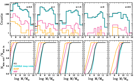
Figure 1: Upper panels: Mass counts of passive galaxies in different redshift bins in the CANDELS deep and wide sample (i.e. all CANDELS except the HUDF area, turquoise), in HUDF (orange), in the HFF data set (magenta), and in the total sample (black). Lower panels: Observational completeness of passive galaxies calculated by means of simulations for the different data sets (same color coding as above). The horizontal dotted lines mark the 75% completeness above which the SMF is computed.

2.1 Photometric catalogs

Our sample comprises the CANDELS (Koekemoer et al., 2011; Grogin et al., 2011) and the Hubble Frontier Fields (HFF, Lotz et al., 2017) programs. Even though CANDELS, with its almost 1000 arcmin², represents a good compromise in terms of area and depth, HFF observations allow us to push the analysis of the SMF further down in stellar mass thanks to the increased statistics at faint magnitudes.

We used the official photometric catalogs (Barro et al., 2019; Galametz et al., 2013; Stefanon et al., 2017; Nayyeri et al., 2017) and the latest photometric redshift release of Kodra et al. (2022) for all CANDELS fields except GOODS-S, for which we adopted the new 43-bands catalog and photo-$z$ of Merlin et al. (2021).

For the HFF we only considered the parallel fields, and used the multiwavelength catalogs, photometric redshifts and lensing factors of Merlin et al. 2016, Castellano et al. 2016 and Di Criscienzo et al. 2017, assembled within the ASTRODEEP project, for A2744, M0416, M0717 and M1149, and of Pagul et al. (2021) for AS1063 and A370. Given the modest lensing amplification in the parallel fields, we considered median magnification values for each field, ranging between 1 and 15% (semi-interquartile ranges cover the interval 3-10%).

The catalogs used in this analysis comprise photometry in 43 (GOODS-S and COSMOS), 18 (GOODS-N), 19 (UDS), 23 (EGS) and 10 (HFF) bands. To homogenize the sample as much as possible, for the AS1063 and A370 HFF catalogs, we used the same bands available for the other 4 fields. The $K$ band and IRAC CH1 and CH2 are available for all catalogs, while the CANDELS sample also includes CH3 and CH4.

2.2 Stellar masses

Stellar masses were estimated by means of SED fitting through the proprietary code zphot (Fontana et al., 2000).

We assumed Bruzual & Charlot (2003) stellar population models, a Chabrier (2003) IMF and delayed star formation histories (SFH($t$)$\propto(t^{2}/\tau)\cdot\exp(-t/\tau)$). The timescale $\tau$ of the declining exponential tail of the SFH ranges from 100 Myr to 7 Gyr, the age can vary between 10 Myr and the age of the Universe at each galaxy redshift, and metallicity can be 0.02, 0.2, 1 and 2.5 times Solar. We assumed a Calzetti et al. (2000) extinction law with E(B-V) varying from 0 to 1.1. Nebular emission is included following the prescriptions of Castellano et al. (2014) and Schaerer & de Barros (2009).

2.3 Sample selections

To ensure reliability of the inferred stellar masses, we cut the sample at a signal to noise ratio (SNR) in the H160 band of at least 5. We report in Table 1 the average total magnitudes corresponding to the adopted SNR threshold in the various subsets, calculated as the median magnitudes of sources with SNR between 4.8 and 5.2.

The sample was cleaned by removing sources affected by photometric issues, X-ray selected AGNs as classified in the CANDELS official catalogs, and stars. These were identified either spectroscopically or photometrically. In the latter case, we removed all sources with SNR(H160)$>$10 and either a) SExtractor (Bertin & Arnouts, 1996) class$\_$star$>$0.95 or b) class$\_$star$>$0.8 and populating the stellar locus of the BzK diagram (Daddi et al., 2004).

2.4 The selection of passive and star-forming galaxies

Passive and star-forming galaxies were identified from their rest-frame ($U$-$V$) and ($V$-$J$) colors (UVJ in the following, Williams et al. 2009). The UVJ selection is widely adopted in the literature and in previous SMF studies (e.g. Muzzin et al., 2013; Tomczak et al., 2014; McLeod et al., 2021). It was shown to agree with a selection based on the specific SFR (e.g. Williams et al., 2009; Carnall et al., 2018, 2019), and the analysis of Whitaker et al. (2013) demonstrated the reliability of UVJ selected quiescent galaxies by means of 3D-HST spectroscopy.

In this work, we adopted the redshift-dependent UVJ cuts of Whitaker et al. (2011). Since the UVJ technique is known to be incomplete in terms of galaxies that have been recently quenched (Merlin et al., 2018; Schreiber et al., 2018; Deshmukh et al., 2018; Carnall et al., 2020), whose abundance is not negligible at $z\gtrsim 3$ due to the short timescales available in the early Universe, we limit our analysis analysis at $z<2.75$.

Tables 2 to 6 show the number of galaxies in each redshift and mass bin for each galaxy population (total, passive and star-forming galaxies). The overall number of sources in each redshift interval is listed in Table 7. Mass counts of passive galaxies in the different redshift bins are shown in Fig. 1.

2.5 The computation of the SMF

We computed the SMF through the non-parametric stepwise method of Castellano et al. (2010), already applied in Santini et al. (2021) (see references and details therein). We assume that the measured density $\phi_{i}^{obs}$ in each mass bin $i$ can be described as the intrinsic density $\phi_{j}^{true}$ in bin $j$ convolved with a transfer function $S_{ij}$.

The transfer function is estimated from simulations performed at the catalog level. Mass counts in each subset (characterized by different photometric properties) are estimated by means of simulations performed ad-hoc and separately for the various fields or sub-fields. These simulations allow us to reconstruct the expected intrinsic (i.e. corrected) mass counts for a given area considering the noise properties of the relevant field.

The simulations are based on Bruzual & Charlot (2003) synthetic templates and were designed to cover the mass range between $10^{5.5}$ and $10^{12.2}M_{\odot}$, to mimic the average photometric noise and the observed mass to light ratio. More specifically, once perturbed with the noise properties of each field and fitted in the same way as real catalogs, mock galaxies were extracted to reproduce the observed mass to flux ratio in the $I$ band in different redshift and mass intervals. To avoid tuning our simulation to data sets that are appreciably affected by incompleteness, we only considered the deep fields, i.e. the Hubble Ultra Deep Field (HUDF)+HFF, for the mass to flux ratio distribution at $\log M/M_{\odot}$$<$8 as well as at $\log M/M_{\odot}$$=$8-9 and $z$$>$2.25, while mock galaxies with $\log M/M_{\odot}$$<$7 were tuned to the observed $\log M/M_{\odot}$$=$7-8 mass bin. For passive and star-forming galaxies, the simulations are based on templates satisfying the relevant UVJ criterion and are tuned to the observed mass to flux ratio distributions of the corresponding population.

Simulated galaxies were treated in exactly the same way as the observed catalogues: they were selected if their SNR in the H160 band is larger than 5 and were classified as passive and star-forming according to their best-fit UVJ colors. For each field, the transfer function $S_{ij}$ was constructed based on the number of simulated galaxies that actually belong to bin $j$ but that, because of noise and systematics, would be observed in bin $i$.

The SMF was finally obtained by inverting the linear system $\phi_{i}^{obs}=\sum_{j}(S_{ij}\phi_{j}^{true})$. This technique takes into account photometric scatter, mass uncertainties (i.e. percolation of sources across adjacent bins), failures in the selection technique and the Eddington bias, without any a-posteriori correction.

Redshift bins were chosen to overlap with the analysis of McLeod et al. (2021), for a cleaner comparison, and mass bins were chosen as a compromise between statistics and mass resolution.

Cosmic variance errors were added in quadrature following the prescriptions adopted in Santini et al. (2021). Briefly, we used the QUICKCV code of Moster et al. (2011), computing relative errors, for a given area, as a function of redshift and stellar mass. Following Driver & Robotham (2010), we reduced these relative errors by $\sqrt{N}$, where $N$ is the number of non-contiguous fields of similar area. We considered $N=5$ for the entire sample (due to the much larger area of each CANDELS field compared to the HFF) and $N=7$ when limiting the analysis to the deeper data (see below). Cosmic variance relative errors range from a few to 15% at the highest redshift and masses. The resulting SMF over five redshift intervals are reported in Tables 2 to 6.

Although the SMF is calculated by solving the linear system above and not correcting the observed densities for the fraction of galaxies that are missing, we can use our simulation to infer an estimate of the sample completeness. The latter is calculated as the fraction of simulated galaxies selected (after treating the simulation in the same way as the real data) in a given mass bin over the total number of input galaxies in the same bin. The resulting completeness is shown in Fig. 1. It is clear how the deepest fields show the higher completeness. In particular, the HUDF and the HFF data are $\sim$100% complete out to M$\sim$$10^{8}M_{\odot}$ ($\sim$$10^{9}M_{\odot}$) at $z<1.5$ ($z>1.5$).

We restricted our analysis to bins where the completeness is above the 75% level, in order to contain potential systematics due to the correction for incompleteness. This effectively limits the bulk of the sample to higher significance, with the SNR distribution peaking at $\sim$10 (instead of 5). As a result of this further cut, the SMF in most of the lowest mass bins was estimated only from the deeper and more complete HFF and HUDF data. Figure 1 shows how the inclusion of the HFF data set is fundamental to probe the low mass regime of the SMF of passive galaxies. While relatively large numbers of candidates are observed in CANDELS, this sample is highly incomplete with respect to this galaxy population at stellar masses below M$\sim$$10^{8.5}M_{\odot}$ ($\sim$$10^{9}M_{\odot}$) at $z<1$ ($z>1$). On the other side, the HUDF alone does not provide sufficient statistics to observe the rare low mass passive galaxies above $z\sim 1.5$.

The stepwise points were fit with a single ($\phi=\ln(10)\times 10^{\phi^{*}_{1}}\times 10^{(\mu-\mu^{*})(\alpha_{1}+1)}\times\exp(-10^{(\mu-\mu^{*})})$) and/or double ($\phi=\ln(10)\times\left[10^{\phi^{*}_{1}}\times 10^{(\mu-\mu^{*})(\alpha_{1}+1)}+10^{\phi^{*}_{2}}\times 10^{(\mu-\mu^{*})(\alpha_{2}+1)}\right]\times\exp(-10^{(\mu-\mu^{*})})$) Schechter function (Weigel et al., 2016), where $\mu=\log M$ and $\mu^{*}=\log M^{*}$. For passive galaxies at $z\sim 2.5$, given the poor sampling in the low mass regime, we fix the faint-end slope to the best-fit value in the previous redshift bin. The best-fit parameters are presented in Table 7.

Field	Area [arcmin2]	F160W 5$\sigma$ limit
GOODS-S HUDF	5.1	29.04
GOODS-S deep	58.9	27.32
GOODS-S ERS	51.5	27.05
GOODS-S wide	53.6	26.44
GOODS-N deep	93.0	27.14
GOODS-N wide	80.0	26.33
UDS	201.7	26.46
EGS	206.0	26.60
COSMOS	216.0	26.69
A2744 parallel	5.0	28.10
M0416 parallel	5.0	28.21
M0717 parallel	6.5	27.75
M1149 parallel	5.3	27.92
AS1063 parallel	6.6	27.63
A370 parallel	5.0	27.94

Table 1: Average 5$\sigma$ limiting total magnitudes in the various fields (or sub-areas of the same field with inhomogeneous coverage), with associated areas. The limiting magnitude was calculated as the median magnitude of sources with SNR between 4.8 and 5.2.

3 Results

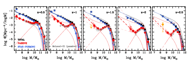
Figure 2: Stellar Mass Function of all (black squares), passive (red solid circles) and star-forming (blue triangles) galaxies. Upper limits are calculated at 1$\sigma$. Solid thick curves show the Schechter fits and the colored shaded areas represent the regions at 68% confidence level considering the joint probability distribution function of the Schechter parameters. Dashed curves indicate the extrapolation of the Schechter fits to lower masses. Thin curves are the two Schechter components of the SMF of passive galaxies. In each panel, dotted curves show the SMF at $z\sim 0.5$. Orange symbols are the results obtained at low masses for passive galaxies using HUDF only (see text), not included in the fits. Gray open circles are the SMF of passive galaxies of McLeod et al. (2021) in the same redshift bins.

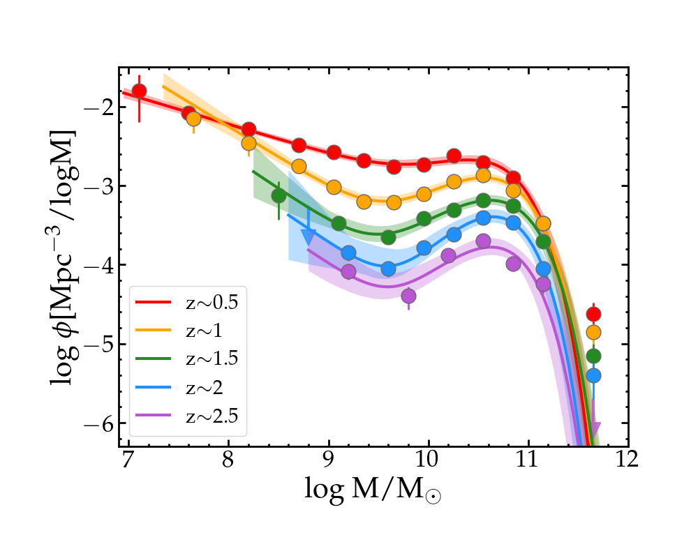
Figure 3: Evolution of the SMF of passive galaxies from $z\sim 2.5$ to $z\sim 0.5$, color-coded as in the legend. Points are the stepwise estimates, solid thick curves show the Schechter fits and the colored shaded areas represent the regions at 68% confidence level considering the joint probability distribution function of the Schechter parameters.

3.1 The evolution of the SMF of passive galaxies

We show in Fig. 2 the SMF of the total sample, of passive and star-forming galaxies, as well as their fits with a Schechter function. The SMF of passive and star-forming galaxies were fit with double and single Schechter functions, respectively. As for the total galaxy population, we compared the single and double Schechter shapes, finding no significant difference in the fits and in the final results. Thus we decided to adopt the parameterization with less free parameters. We note that the upper limit measured in the lowest mass bin of the SMF of passive galaxies at $z\sim 2$ results from an almost complete lack of counts in that redshift and mass range in the HUDF+HFF sample (see Fig. 1). This can be ascribed to a combination of small statistics and cosmic variance. Although many more passive galaxies are selected in the same interval in the deep and wide CANDELS fields, we did not used them due to the high incompleteness level of the parent sample.

We also note that the exact low-mass slope of the SMF of passive galaxies may vary as a consequence of sample selection and mass binning choice, especially in the highest redshift bins, and will be better constrained with deeper JWST observations. However, the presence of a low mass population of passive galaxies is a solid result at all redshifts probed. As a matter of fact, the $10^{9}-10^{9.2}M_{\odot}$ points of the SMF are above the extrapolation of a single Schechter fit to the high mass points by 0.5-0.8 dex and inconsistent with it at a 4-8$\sigma$ confidence level, with these deviations and inconsistencies increasing as the stellar mass decreases.

While the SMF of star-forming and total galaxies only evolve mildly over the redshift range probed by the present work, the strong evolution observed for the passive sample suggests a continuous and significant build-up for this galaxy population over the last $\sim$11 Gyr (see also Santini et al., 2021, and references therein). Figure 3 shows the five redshift bins on the same panel to better visualize the evolution in the SMF of passive galaxies, amounting to more than an order of magnitude from $z\sim 2.5$ to $z\sim 0.5$ at fixed stellar mass. As might be expected, the Stellar Mass Density (SMD), obtained by integrating the best-fit Schechter functions above $10^{8}M_{\odot}$, shows a similar evolutionary trend (Fig. 4). Passive galaxies account for 60% of the total mass in the nearby Universe, but for only $\sim$20% at $z\sim 2.5$, in agreement with previous results (Muzzin et al., 2013; Ilbert et al., 2013; Straatman et al., 2014; Tomczak et al., 2014; Mortlock et al., 2015; Davidzon et al., 2017; McLeod et al., 2021). Over the redshift interval probed by our analysis, the SMD of passive galaxies increases by more than a factor of 10 (within the range 6-20 at 1$\sigma$), compared to a factor of $\sim$3 and $\sim$1.5 evolution experienced by the total galaxy population and the star-forming subsample, respectively.

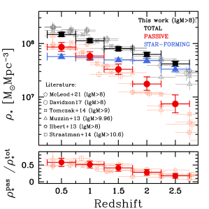
Figure 4: Upper panel: evolution of the Stellar Mass Density at $M>10^{8}M_{\odot}$ of all (solid black squares), passive (solid red circles) and star-forming (solid blue triangles) galaxies. Open black and reddish symbols show previous results from the literature, according to the legend, for all and passive galaxies, respectively. Lower panel: ratio of the SMD of passive galaxies to the overall galaxy population at $M>10^{8}M_{\odot}$, compared to the literature (symbols are as in the upper panel).

As discussed above, we observe clear evidence of an upturn at low stellar masses in the SMF of the passive galaxy sample at all redshifts probed by our analyses. This upturn has already been identified in the local Universe (e.g., Baldry et al., 2012) and at $z\lesssim 1.5$ (Tomczak et al., 2014; Mortlock et al., 2015; Davidzon et al., 2017; McLeod et al., 2021), but was never observed before at such high redshifts. We compared our SMF with the recent results of McLeod et al. (2021) (Fig. 2), which include CANDELS data, along with ground-based surveys, and a correction for incompleteness in the selection of passive galaxies, though with a different technique. We found good agreement in the common mass range, even at the high-mass end despite the much larger area probed by their work. The inclusion of the deep HFF data, however, allow us to push the analysis below $\log M/M_{\odot}$$\sim$9.5 at $z>1.5$ and to probe the existence of a secondary population of passive galaxies arising at low masses already at these early epochs. Indeed, as shown by Fig. 1 and discussed in Sect. 2.5, the above mass range is only poorly sampled by the deepest CANDELS data, with the HUDF area suffering from much lower statistics and larger cosmic variance than the full HUDF+HFF deep sample used in this work.

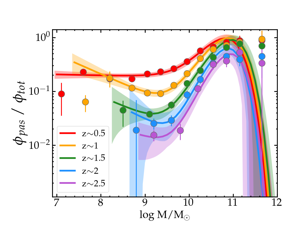
Figure 5: Ratio of the SMF of passive to total galaxies at different redshifts, color-coded as in the legend. Symbols and curves show the ratio of the stepwise points and of the Schechter fits, respectively.

Despite the poor statistics, in the attempt of investigating even lower masses, we also calculated the SMF of passive galaxies from the HUDF alone exploiting its higher depth compared to the HFF program. As can be seen on Fig. 1, the completeness in HUDF is indeed higher than for HFF. The difference is more pronounced at $z\sim 2.5$, likely as a consequence of deeper IRAC photometry allowing a more accurate UVJ selection at high redshift. When the completeness is above the chosen threshold and the sparse HUDF counts allow us to estimate the SMF in a mass regime not probed by the combination of HUDF+HFF, we show the stepwise results on Fig. 2 as orange symbols. Although we do not use these points in the fits because of the poor statistics and large field-to-field variation, they corroborate the existence of a low mass population of passive galaxies at the highest redshifts probed by our analysis.

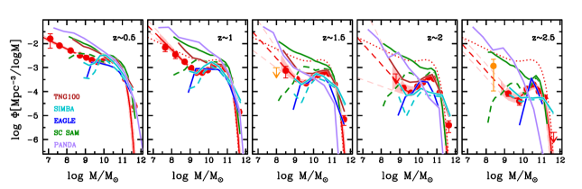
Figure 6: Stellar Mass Function of passive galaxies (in red, as shown in Fig. 2) compared to a set of theoretical predictions (see text and legend). Dashed lines show the Santa Cruz (green) and SIMBA (light blue) models after satellite galaxies have been removed. Theoretical predictions are only shown above their mass completeness limit (see text), and predictions of zero galaxies have not been plotted.

We run several simulations to rule out the possibility that the low-mass turnover is caused by a population of dusty star-forming galaxies misinterpreted as passive. Firstly, we produced a mock catalog of galaxies reproducing the photometric properties of one of the deep fields (we considered A2744), on which the estimate of the SMF at low masses is mostly based. We considered models with E(B-V) in the range 0.5-1.1, normalized them to a H160 magnitude from 25 to 28, perturbed them with noise and fitted them with the same stellar library adopted to calculate the physical properties of our galaxies. We estimated the contamination as a function of stellar mass, and found a roughly mass-independent value of 10-30% (we checked that lower values of extinction cause only a few per cent contamination at $z\lesssim 1.5$). On the basis of these results, starting from the observed number of passive galaxies and dusty ones (with different levels of extinction), we estimated an effective contamination ranging from a few to 10% level at $M<10^{9}M_{\odot}$ and $\sim 20-40\%$ at intermediate masses ($M\sim 10^{9}-10^{10}M_{\odot}$), due to the lower number of passive galaxies in this mass range. Secondly, we considered the observed galaxy sample in A2744 independently on their dust obscuration, replicated it 10 times to increase the statistics, perturbed its photometry according to the typical noise properties of that field and fitted it in the usual way. We found a contamination of the order of 10% at $z<2$ and 20-30% at higher redshift. These levels of contamination, while potentially affecting the exact value of the slope of the SMF, do not change our main conclusion. Moreover, according to these tests, the contamination from dusty galaxies would make the slope of the low-mass component shallower rather than steeper.

3.2 Two populations of passive galaxies

The shape of the SMF and its evolution point to the existence of two different populations of passive galaxies down to $z\sim 2.75$. The abundances of low- and high-mass passive galaxies evolve at markedly different rates: from $z\sim 2.5$ to $z\sim 0.5$ we observe an evolution by a factor of $\sim$20 and $\sim$6 at $\log M/M_{\odot}$$\sim$9 and $\sim 11$, respectively. A similar behaviour is shown by the Schechter fits: the normalization of the high- and low-mass components, $\phi_{*1}$ and $\phi_{*2}$, evolve by one and two orders of magnitude, respectively (see Table 7).

To assess the mutual importance of the two quenching modes expected to be at work in the low and high mass regime, it is interesting to evaluate the fraction of passive galaxies as a function of time and stellar mass. To this aim, Fig. 5 shows the ratio of the SMF of passive to total galaxies at each given redshift. Compared to the total population, passive galaxies underwent a differential evolution with stellar mass: while the majority of massive ($\log M/M_{\odot}$$>$11-11.5) systems were already passive at $z$$\sim$ 2, and almost 50% of them even at $z$$\sim$ 2.5, the fraction of low mass ($\log M/M_{\odot}$$<$10) passive galaxies experienced more than a factor of 10 evolution between $z\sim 2-2.5$ and the present epoch. These findings, discussed in the next section, qualitatively agree with previous studies at similar redshifts (e.g. Fontana et al., 2009; Ilbert et al., 2013; Muzzin et al., 2013; Tomczak et al., 2014; Mortlock et al., 2015; McLeod et al., 2021).

4 Discussion

In empirical and theoretical models, the evolution of the passive population is driven by a set of physical effects. In the empirical model of Peng et al. (2010), the two populations arise as a result of two different quenching processes: the mass-quenching mode, dominant at high masses, and environmental-quenching, responsible for the upturn characterizing the low mass end.

Massive galaxies reside in biased regions of the density field, have started forming their stars earlier and have become passive at an earlier time, in agreement with a downsizing scenario (e.g. Cowie et al., 1996; Fontanot et al., 2009). Moreover, cooling is inefficient in high mass systems, hampering gas re-accretion and new star formation episodes once the galaxy has run out of gas. Conversely, gas is continuously expelled and re-accreted by low mass galaxies in the field thanks to rapid and efficient cooling, giving rise to a more prolonged star formation period and delayed quenching. However, low-mass galaxies are quenched by environmental effects (e.g. Fossati et al., 2017; Papovich et al., 2018; Xie et al., 2020), as they enter in the virialized structures that progressively came into place ($z\sim 2$, e.g. Overzier, 2016). This results in a differential evolution of the SMF of passive galaxies due to the time-evolving role of the environment in suppressing the star formation, which becomes increasingly more important at later epochs. Similar conclusions on the evolution of environmental quenching processes are supported by both theoretical models (van de Voort et al., 2017) and observations (Kawinwanichakij et al., 2017).

This differential evolution is exactly the central finding of this work, as shown in Figs. 3 and 5. We cannot demonstrate that the low-mass part of the SMF is dominated by satellite galaxies in dense environments, as this would require an identification of the environment in which each galaxy reside, which is beyond the goal of this work. However, we do find that the SMF of massive galaxies is largely in place already at $z\simeq 2$, while the low–mass part grows in subsequent times, lending support to the environmental explanation for the growth of the low-mass side.

4.1 Comparison with theoretical predictions

To further explore the origin of the SMF of passive galaxies and the connection of the low-mass upturn with the environment, we have performed a comparison with theoretical predictions. In Fig. 6 we compare our results with several models: the semianalytic model PANDA (Menci et al., 2019), the mock lightcones extracted from the semianalytic Santa Cruz model (Somerville et al., 2021), and three hydrodynamic simulations, namely IllustrisTNG100 (Pillepich et al., 2018; Nelson et al., 2019), EAGLE (Schaye et al., 2015) and SIMBA (Davé et al., 2019). Passive galaxies in the models were selected from the simulated rest-frame $U$, $V$ and $J$ magnitudes, adopting the very same cuts used on the data. TNG100 does not provide this information at $z>2$, so we did not include it in our highest redshift bin. We plot the model predictions above their mass completeness limits. The PANDA model does not suffer from incompleteness, as the dark matter halo merging histories are based on a Monte Carlo procedure and go down to $10^{5}M_{\odot}$. The Santa Cruz model is complete above $2.2\times 10^{10}M_{\odot}$ in halo mass; following Somerville et al. (2021), we only show the SMF above $10^{8}M_{\odot}$. The minimum stellar mass of a resolved galaxy in TNG100, EAGLE and SIMBA is $1.4\times 10^{8}$, $2\times 10^{8}$ and $5.8\times 10^{8}M_{\odot}$, respectively (for TNG100 we used the highest resolution simulation, i.e. TNG100-1).

In general, we see from Fig. 6 that models hardly reproduce the population of passive galaxies beyond the local Universe, as also seen at even higher redshift in Santini et al. (2021). The various predictions correctly model certain redshift or mass intervals, including simulating the low and high mass populations; in particular, SIMBA, and to a lesser extent TNG100, well reproduce the low-mass upturn at $z\sim 1.5-2$. However, none of the models are able to match the observations over the entire redshift and stellar mass dynamical range probed, suggesting that the physical processes involved with the formation of passive galaxies are still not well understood.

Hydrodynamical simulations may underpredict the faint end of the SMF depending on the adopted mass resolution, yielding to zero galaxies below a given threshold and truncated SMF (TNG100 makes an exception, thanks to its slightly higher resolution and the adoption of the moving-mesh method for solving the hydrodynamical equations, Pillepich et al. 2018). Additionally, an inefficient feedback description is likely responsible for the lack of passive sources in EAGLE, in particular at the lowest masses, as well as in SIMBA at intermediate masses and $z\geq 1.5$.

Conversely, a common flaw of semianalytic models is their overproduction of low mass passive galaxies as a consequence of the introduction of efficient mechanisms to suppress excessive star formation and mass production at high redshift. The overestimate of the number of passive sources can be ascribed to the implementation of gas stripping in satellite galaxies, which is usually described as an instantaneous process in the models (but see Henriques et al. 2017 for a partial solution to this problem), resulting in an unrealistically rapid process. This therefore invokes the need for improving the description of the environmental processes in the models, in particular in satellite galaxies (see also Calabrò et al. 2022).

From the Santa Cruz model and from the SIMBA simulation we also extracted information on the environment in which each galaxy resides. Following Somerville et al. (2021), we identified satellites by selecting the galaxies flagged as belonging to a dark matter sub-halo, i.e. a halo that have become subsumed within another virialized halo and that is tidally stripped as it orbits within its host halo. As for SIMBA, we used the flag identifying the highest stellar mass galaxy as central, and all other galaxies in the same halo as satellites. With this information, we estimated the SMF of central galaxies only. It is clear from Fig. 6 (dashed lines) that the predicted SMF of passive galaxies at high masses drops when satellite galaxies are removed, consistently with the results of Donnari et al. (2021) (we note however that this effect is milder in SIMBA at $z\geq 1.5$, likely due to resolution issues at the lowest masses and lower efficiency feedback processes in the satellites at $z\sim 2.5$ relative to centrals). Since environmental effects such as ram-pressure or tidal stripping are expected to operate on low-mass satellites, on the basis of both observations (e.g. Kovač et al., 2014; Tal et al., 2014; Wetzel et al., 2015; Papovich et al., 2018) and simulations (Fillingham et al., 2018; Samuel et al., 2022), this result supports the interpretation of the environment as major contributor in shaping the SMF of passive galaxies at low masses.

5 Summary and conclusions

Reliable observations over a wide range of masses are crucial to constrain the delicate processes responsible for the formation of passive galaxies and improve their description in the models, in order to advance our understanding of the galaxy evolution scenario. Thanks to the inclusion of the deep HFF data in our sample, as a complement to the CANDELS dataset, we were able to trace the evolution of the SMF at low masses up to $z$$<$2.75.

The observed shape of the SMF points to the existence of two populations of passive galaxies that underwent different quenching mechanisms and are characterized by different evolutionary timescales. Over the entire redshift range, and for the first time at $z$$>$1.5, we observe the build-up of the low mass component, thought to originate from environmental effects, efficient at suppressing the star formation in low mass galaxies.

JWST observations that are rapidly becoming available will allow the sampling of the $\log M/M_{\odot}\lesssim 9$ regime at $z\gtrsim 2$ with high accuracy (less than a factor of 2 uncertainty on the stellar mass). This will reduce the current uncertainty on the low-mass side of the SMF and will allow us to push the analysis to even higher redshift. Accurate observational results will allow us to better constrain the theoretical description of the physical processes at play, with the final aim of better understanding the role of environment, and its evolution with cosmic time, in suppressing the star formation in galaxies.

$0.25<z<0.75$
$\log M$	$N_{all}$	$\log\phi_{all}$	$N_{pas}$	$\log\phi_{pas}$	$N_{sf}$	$\log\phi_{sf}$
7.10	294∗	-0.75${}_{-0.05}^{+0.04}$	43∗	-1.80${}_{-0.40}^{+0.20}$	251∗	-0.82${}_{-0.05}^{+0.04}$
7.60	8730	-1.44${}_{-0.02}^{+0.02}$	1165	-2.08${}_{-0.03}^{+0.03}$	7565	-1.51${}_{-0.02}^{+0.02}$
8.20	7952	-1.52${}_{-0.02}^{+0.02}$	1363	-2.29${}_{-0.03}^{+0.02}$	6589	-1.60${}_{-0.02}^{+0.02}$
8.70	3360	-1.72${}_{-0.02}^{+0.02}$	644	-2.49${}_{-0.03}^{+0.03}$	2716	-1.82${}_{-0.02}^{+0.02}$
9.05	1660	-1.90${}_{-0.03}^{+0.02}$	343	-2.58${}_{-0.04}^{+0.03}$	1317	-2.00${}_{-0.03}^{+0.02}$
9.35	1195	-2.05${}_{-0.03}^{+0.02}$	283	-2.68${}_{-0.04}^{+0.04}$	912	-2.17${}_{-0.03}^{+0.03}$
9.65	886	-2.18${}_{-0.03}^{+0.03}$	233	-2.76${}_{-0.04}^{+0.04}$	653	-2.31${}_{-0.03}^{+0.03}$
9.95	718	-2.28${}_{-0.03}^{+0.03}$	273	-2.73${}_{-0.04}^{+0.04}$	445	-2.49${}_{-0.03}^{+0.03}$
10.25	571	-2.38${}_{-0.03}^{+0.03}$	308	-2.62${}_{-0.04}^{+0.03}$	263	-2.71${}_{-0.04}^{+0.04}$
10.55	398	-2.54${}_{-0.04}^{+0.03}$	265	-2.71${}_{-0.04}^{+0.04}$	133	-3.01${}_{-0.05}^{+0.04}$
10.85	213	-2.81${}_{-0.04}^{+0.04}$	173	-2.90${}_{-0.04}^{+0.04}$	40	-3.54${}_{-0.08}^{+0.07}$
11.15	53	-3.42${}_{-0.08}^{+0.07}$	47	-3.47${}_{-0.08}^{+0.07}$	6	-4.36${}_{-0.23}^{+0.15}$
11.65	9	-4.57${}_{-0.18}^{+0.12}$	8	-4.62${}_{-0.20}^{+0.14}$	1	$<$5.52

Table 2: Stellar Mass Function of all, passive and star-forming galaxies as calculated with the stepwise method in the $0.25<z<0.75$ redshift interval. The 1$\sigma$ uncertainties include Poissonian errors and cosmic variance. Stellar masses are in Solar masses and the SMF are in units of 1/Mpc³/dex. Columns 2, 4 and 6 indicate the number of sources in each bin. Asterisks denote the bins for which the SMF has been estimated from the HUDF+HFF data sets only to have a cleaner measurement thanks to the higher level of completeness.

$0.75<z<1.25$
$\log M$	$N_{all}$	$\log\phi_{all}$	$N_{pas}$	$\log\phi_{pas}$	$N_{sf}$	$\log\phi_{sf}$
7.15	311∗	-1.13${}_{-0.05}^{+0.05}$	–	–	308∗	-1.14${}_{-0.05}^{+0.05}$
7.65	448∗	-0.96${}_{-0.04}^{+0.03}$	18∗	-2.16${}_{-0.18}^{+0.13}$	430∗	-0.97${}_{-0.04}^{+0.03}$
8.20	10174	-1.70${}_{-0.02}^{+0.02}$	21∗	-2.46${}_{-0.17}^{+0.12}$	9623	-1.74${}_{-0.02}^{+0.02}$
8.70	5912	-1.82${}_{-0.02}^{+0.02}$	448	-2.76${}_{-0.03}^{+0.03}$	5464	-1.85${}_{-0.02}^{+0.02}$
9.05	2978	-1.98${}_{-0.02}^{+0.02}$	277	-3.01${}_{-0.04}^{+0.04}$	2701	-2.03${}_{-0.02}^{+0.02}$
9.35	2014	-2.16${}_{-0.02}^{+0.02}$	189	-3.21${}_{-0.05}^{+0.05}$	1825	-2.20${}_{-0.02}^{+0.02}$
9.65	1425	-2.32${}_{-0.02}^{+0.02}$	205	-3.21${}_{-0.05}^{+0.04}$	1220	-2.38${}_{-0.02}^{+0.02}$
9.95	1125	-2.44${}_{-0.02}^{+0.02}$	266	-3.10${}_{-0.04}^{+0.04}$	859	-2.54${}_{-0.03}^{+0.02}$
10.25	833	-2.56${}_{-0.03}^{+0.03}$	358	-2.95${}_{-0.04}^{+0.03}$	475	-2.79${}_{-0.03}^{+0.03}$
10.55	660	-2.65${}_{-0.03}^{+0.03}$	394	-2.87${}_{-0.03}^{+0.03}$	266	-3.04${}_{-0.04}^{+0.03}$
10.85	363	-2.92${}_{-0.03}^{+0.03}$	250	-3.06${}_{-0.04}^{+0.04}$	113	-3.42${}_{-0.05}^{+0.04}$
11.15	118	-3.39${}_{-0.06}^{+0.05}$	98	-3.48${}_{-0.06}^{+0.05}$	20	-4.16${}_{-0.12}^{+0.10}$
11.65	11	-4.82${}_{-0.18}^{+0.12}$	10	-4.85${}_{-0.15}^{+0.11}$	1	$<$6.00

Table 3: Same as Table 2 for the $0.75<z<1.25$ redshift interval.

$1.25<z<1.75$
$\log M$	$N_{all}$	$\log\phi_{all}$	$N_{pas}$	$\log\phi_{pas}$	$N_{sf}$	$\log\phi_{sf}$
8.00	322∗	-1.16${}_{-0.05}^{+0.04}$	–	–	319∗	-1.16${}_{-0.05}^{+0.04}$
8.50	10613	-1.77${}_{-0.02}^{+0.02}$	6∗	-3.12${}_{-0.31}^{+0.18}$	10421	-1.80${}_{-0.02}^{+0.02}$
9.10	6781	-2.05${}_{-0.02}^{+0.02}$	232	-3.47${}_{-0.04}^{+0.04}$	6549	-2.07${}_{-0.02}^{+0.02}$
9.60	2106	-2.40${}_{-0.02}^{+0.02}$	135	-3.65${}_{-0.06}^{+0.06}$	1971	-2.42${}_{-0.02}^{+0.02}$
9.95	1095	-2.57${}_{-0.03}^{+0.02}$	167	-3.42${}_{-0.05}^{+0.05}$	928	-2.63${}_{-0.03}^{+0.02}$
10.25	791	-2.70${}_{-0.03}^{+0.03}$	211	-3.31${}_{-0.05}^{+0.04}$	580	-2.82${}_{-0.03}^{+0.03}$
10.55	585	-2.82${}_{-0.03}^{+0.03}$	268	-3.19${}_{-0.04}^{+0.04}$	317	-3.08${}_{-0.04}^{+0.03}$
10.85	326	-3.07${}_{-0.04}^{+0.03}$	203	-3.25${}_{-0.04}^{+0.04}$	123	-3.50${}_{-0.05}^{+0.05}$
11.15	97	-3.59${}_{-0.06}^{+0.06}$	72	-3.71${}_{-0.07}^{+0.06}$	25	-4.18${}_{-0.10}^{+0.08}$
11.65	9	-5.00${}_{-0.15}^{+0.11}$	7	-5.15${}_{-0.24}^{+0.15}$	2	$<$5.70

Table 4: Same as Table 2 for the $1.25<z<1.75$ redshift interval.

$1.75<z<2.25$
$\log M$	$N_{all}$	$\log\phi_{all}$	$N_{pas}$	$\log\phi_{pas}$	$N_{sf}$	$\log\phi_{sf}$
8.30	5822	-2.02${}_{-0.02}^{+0.02}$	–	–	5783	-2.02${}_{-0.02}^{+0.02}$
8.80	4482	-2.10${}_{-0.02}^{+0.02}$	1∗	$<$-3.26	4434	-2.11${}_{-0.02}^{+0.02}$
9.20	3129	-2.25${}_{-0.02}^{+0.02}$	44	-3.84${}_{-0.11}^{+0.09}$	3085	-2.25${}_{-0.02}^{+0.02}$
9.60	1790	-2.52${}_{-0.03}^{+0.02}$	56	-4.05${}_{-0.10}^{+0.08}$	1734	-2.53${}_{-0.03}^{+0.02}$
9.95	826	-2.72${}_{-0.03}^{+0.03}$	89	-3.79${}_{-0.08}^{+0.07}$	737	-2.77${}_{-0.03}^{+0.03}$
10.25	627	-2.84${}_{-0.03}^{+0.03}$	115	-3.62${}_{-0.07}^{+0.06}$	512	-2.92${}_{-0.03}^{+0.03}$
10.55	517	-2.92${}_{-0.04}^{+0.04}$	180	-3.40${}_{-0.05}^{+0.05}$	337	-3.10${}_{-0.04}^{+0.04}$
10.85	322	-3.12${}_{-0.04}^{+0.04}$	136	-3.47${}_{-0.05}^{+0.05}$	186	-3.36${}_{-0.05}^{+0.04}$
11.15	91	-3.65${}_{-0.07}^{+0.06}$	36	-4.05${}_{-0.10}^{+0.08}$	55	-3.86${}_{-0.08}^{+0.07}$
11.65	9	-5.05${}_{-0.18}^{+0.12}$	4	-5.40${}_{-0.30}^{+0.18}$	5	-5.30${}_{-0.22}^{+0.15}$

Table 5: Same as Table 2 for the $1.75<z<2.25$ redshift interval.

$2.25<z<2.75$
$\log M$	$N_{all}$	$\log\phi_{all}$	$N_{pas}$	$\log\phi_{pas}$	$N_{sf}$	$\log\phi_{sf}$
8.40	547∗	-1.78${}_{-0.04}^{+0.04}$	–	–	540∗	-1.81${}_{-0.04}^{+0.04}$
9.20	6002	-2.27${}_{-0.02}^{+0.02}$	145	-4.08${}_{-0.11}^{+0.09}$	5857	-2.28${}_{-0.02}^{+0.02}$
9.80	1320	-2.67${}_{-0.03}^{+0.03}$	34	-4.40${}_{-0.17}^{+0.12}$	1286	-2.68${}_{-0.03}^{+0.03}$
10.20	671	-2.94${}_{-0.03}^{+0.03}$	90	-3.89${}_{-0.07}^{+0.06}$	581	-2.99${}_{-0.04}^{+0.03}$
10.55	280	-3.20${}_{-0.05}^{+0.05}$	88	-3.69${}_{-0.07}^{+0.06}$	192	-3.37${}_{-0.06}^{+0.05}$
10.85	126	-3.55${}_{-0.06}^{+0.05}$	46	-3.99${}_{-0.09}^{+0.08}$	80	-3.75${}_{-0.07}^{+0.06}$
11.15	45	-3.97${}_{-0.10}^{+0.08}$	22	-4.24${}_{-0.12}^{+0.10}$	23	-4.26${}_{-0.13}^{+0.10}$
11.65	3	-5.52${}_{-0.48}^{+0.22}$	1	$<$6.00	2	-5.70${}_{-0.30}^{+0.18}$

Table 6: Same as Table 2 for the $2.25<z<2.75$ redshift interval.

Redshift	N	$\log M^{*}/M_{\odot}$	$\alpha_{1}$	$\log\phi_{*1}$/Mpc-3	$\alpha_{2}$	$\log\phi_{*2}$/Mpc-3	$\log\rho_{>8}/(M_{\odot}$Mpc-3)
All galaxies
0.25 - 0.75	26039	10.98 $\pm$ 0.03	-1.36 $\pm$ 0.01	-2.96 $\pm$ 0.03	–	–	8.17${}_{-0.04}^{+0.04}$
0.75 - 1.25	26372	11.08 $\pm$ 0.03	-1.41 $\pm$ 0.01	-3.20 $\pm$ 0.03	–	–	8.05${}_{-0.03}^{+0.03}$
1.25 - 1.75	22725	11.11 $\pm$ 0.03	-1.50 $\pm$ 0.01	-3.45 $\pm$ 0.04	–	–	7.90${}_{-0.03}^{+0.03}$
1.75 - 2.25	17615	11.10 $\pm$ 0.03	-1.45 $\pm$ 0.01	-3.50 $\pm$ 0.04	–	–	7.80${}_{-0.04}^{+0.04}$
2.25 - 2.75	8994	11.05 $\pm$ 0.06	-1.61 $\pm$ 0.03	-3.76 $\pm$ 0.07	–	–	7.62${}_{-0.05}^{+0.05}$
Passive galaxies
0.25 - 0.75	5148	10.54 $\pm$ 0.06	-0.06 $\pm$ 0.18	-2.67 $\pm$ 0.04	-1.38 $\pm$ 0.03	-3.54 $\pm$ 0.09	7.93${}_{-0.08}^{+0.08}$
0.75 - 1.25	2534	10.59 $\pm$ 0.05	-0.04 $\pm$ 0.13	-2.84 $\pm$ 0.03	-1.77 $\pm$ 0.08	-4.61 $\pm$ 0.18	7.77${}_{-0.08}^{+0.08}$
1.25 - 1.75	1301	10.62 $\pm$ 0.06	-0.00 $\pm$ 0.18	-3.12 $\pm$ 0.03	-1.85 $\pm$ 0.31	-5.21 $\pm$ 0.55	7.52${}_{-0.10}^{+0.10}$
1.75 - 2.25	661	10.48 $\pm$ 0.07	0.47 $\pm$ 0.30	-3.37 $\pm$ 0.04	-1.85 $\pm$ 0.64	-5.34 $\pm$ 0.86	7.24${}_{-0.12}^{+0.13}$
2.25 - 2.75	426	10.52 $\pm$ 0.10	0.31 $\pm$ 0.29	-3.73 $\pm$ 0.04	-1.85 $\pm$ 0.00	-5.64 $\pm$ 0.18	6.87${}_{-0.16}^{+0.17}$
Star-forming galaxies
0.25 - 0.75	20891	10.60 $\pm$ 0.04	-1.42 $\pm$ 0.01	-3.01 $\pm$ 0.04	–	–	7.76${}_{-0.04}^{+0.04}$
0.75 - 1.25	23305	10.72 $\pm$ 0.03	-1.45 $\pm$ 0.01	-3.18 $\pm$ 0.04	–	–	7.74${}_{-0.03}^{+0.03}$
1.25 - 1.75	21235	10.81 $\pm$ 0.04	-1.53 $\pm$ 0.02	-3.36 $\pm$ 0.05	–	–	7.69${}_{-0.03}^{+0.03}$
1.75 - 2.25	16868	11.04 $\pm$ 0.04	-1.49 $\pm$ 0.02	-3.59 $\pm$ 0.04	–	–	7.68${}_{-0.04}^{+0.04}$
2.25 - 2.75	8561	10.89 $\pm$ 0.07	-1.63 $\pm$ 0.03	-3.71 $\pm$ 0.08	–	–	7.52${}_{-0.05}^{+0.05}$

Table 7: Best-fit parameters and their 1$\sigma$ uncertainties in the different redshift intervals derived from fitting the stepwise SMF with a single or double Schechter function for all galaxies and for the passive and star-forming populations. The second column indicates the numbers of galaxies used for computing the SMF in each redshift bin. The last column reports the corresponding mass density $\rho$ obtained by integrating the SMF above $10^{8}M_{\odot}$. We note that for passive galaxies at $z\sim 2.5$, $\alpha_{2}$ was fixed to the best-fit value in the previous redshift interval.

References

- Baldry et al. (2012) Baldry, I. K., Driver, S. P., Loveday, J., et al. 2012, MNRAS, 421, 621, doi: 10.1111/j.1365-2966.2012.20340.x
- Barro et al. (2019) Barro, G., Pérez-González, P. G., Cava, A., et al. 2019, ApJS, 243, 22, doi: 10.3847/1538-4365/ab23f2
- Bertin & Arnouts (1996) Bertin, E., & Arnouts, S. 1996, A&AS, 117, 393
- Brinchmann et al. (2004) Brinchmann, J., Charlot, S., White, S. D. M., et al. 2004, MNRAS, 351, 1151, doi: 10.1111/j.1365-2966.2004.07881.x
- Brown et al. (2017) Brown, T., Catinella, B., Cortese, L., et al. 2017, MNRAS, 466, 1275, doi: 10.1093/mnras/stw2991
- Bruzual & Charlot (2003) Bruzual, G., & Charlot, S. 2003, MNRAS, 344, 1000, doi: 10.1046/j.1365-8711.2003.06897.x
- Calabrò et al. (2022) Calabrò, A., Guaita, L., Pentericci, L., et al. 2022, arXiv e-prints, arXiv:2203.04934. https://arxiv.org/abs/2203.04934
- Calzetti et al. (2000) Calzetti, D., Armus, L., Bohlin, R. C., et al. 2000, ApJ, 533, 682, doi: 10.1086/308692
- Carnall et al. (2018) Carnall, A. C., McLure, R. J., Dunlop, J. S., & Davé, R. 2018, MNRAS, 480, 4379, doi: 10.1093/mnras/sty2169
- Carnall et al. (2019) Carnall, A. C., McLure, R. J., Dunlop, J. S., et al. 2019, MNRAS, 490, 417, doi: 10.1093/mnras/stz2544
- Carnall et al. (2020) Carnall, A. C., Walker, S., McLure, R. J., et al. 2020, MNRAS, 496, 695, doi: 10.1093/mnras/staa1535
- Castellano et al. (2010) Castellano, M., Fontana, A., Paris, D., et al. 2010, A&A, 524, A28+, doi: 10.1051/0004-6361/201015195
- Castellano et al. (2014) Castellano, M., Sommariva, V., Fontana, A., et al. 2014, A&A, 566, A19, doi: 10.1051/0004-6361/201322704
- Castellano et al. (2016) Castellano, M., Amorín, R., Merlin, E., et al. 2016, A&A, 590, A31, doi: 10.1051/0004-6361/201527514
- Chabrier (2003) Chabrier, G. 2003, ApJ, 586, L133, doi: 10.1086/374879
- Cowie et al. (1996) Cowie, L. L., Songaila, A., Hu, E. M., & Cohen, J. G. 1996, AJ, 112, 839, doi: 10.1086/118058
- Daddi et al. (2004) Daddi, E., Cimatti, A., Renzini, A., et al. 2004, ApJ, 617, 746, doi: 10.1086/425569
- Davé et al. (2019) Davé, R., Anglés-Alcázar, D., Narayanan, D., et al. 2019, MNRAS, 486, 2827, doi: 10.1093/mnras/stz937
- Davidzon et al. (2017) Davidzon, I., Ilbert, O., Laigle, C., et al. 2017, A&A, 605, A70, doi: 10.1051/0004-6361/201730419
- Deshmukh et al. (2018) Deshmukh, S., Caputi, K. I., Ashby, M. L. N., et al. 2018, ApJ, 864, 166, doi: 10.3847/1538-4357/aad9f5
- Di Criscienzo et al. (2017) Di Criscienzo, M., Merlin, E., Castellano, S., et al. 2017, A&A, submitted
- Donnari et al. (2021) Donnari, M., Pillepich, A., Nelson, D., et al. 2021, MNRAS, 506, 4760, doi: 10.1093/mnras/stab1950
- Driver & Robotham (2010) Driver, S. P., & Robotham, A. S. G. 2010, MNRAS, 407, 2131, doi: 10.1111/j.1365-2966.2010.17028.x
- Elbaz et al. (2007) Elbaz, D., Daddi, E., Le Borgne, D., et al. 2007, A&A, 468, 33, doi: 10.1051/0004-6361:20077525
- Farouki & Shapiro (1981) Farouki, R., & Shapiro, S. L. 1981, ApJ, 243, 32, doi: 10.1086/158563
- Fillingham et al. (2018) Fillingham, S. P., Cooper, M. C., Boylan-Kolchin, M., et al. 2018, MNRAS, 477, 4491, doi: 10.1093/mnras/sty958
- Fontana et al. (2000) Fontana, A., D’Odorico, S., Poli, F., et al. 2000, AJ, 120, 2206, doi: 10.1086/316803
- Fontana et al. (2009) Fontana, A., Santini, P., Grazian, A., et al. 2009, A&A, 501, 15, doi: 10.1051/0004-6361/200911650
- Fontanot et al. (2009) Fontanot, F., De Lucia, G., Monaco, P., Somerville, R. S., & Santini, P. 2009, MNRAS, 397, 1776, doi: 10.1111/j.1365-2966.2009.15058.x
- Fossati et al. (2017) Fossati, M., Wilman, D. J., Mendel, J. T., et al. 2017, ApJ, 835, 153, doi: 10.3847/1538-4357/835/2/153
- Galametz et al. (2013) Galametz, A., Grazian, A., Fontana, A., et al. 2013, ApJS, 206, 10, doi: 10.1088/0067-0049/206/2/10
- Geha et al. (2012) Geha, M., Blanton, M. R., Yan, R., & Tinker, J. L. 2012, ApJ, 757, 85, doi: 10.1088/0004-637X/757/1/85
- Grogin et al. (2011) Grogin, N. A., Kocevski, D. D., Faber, S. M., et al. 2011, ApJS, 197, 35. https://arxiv.org/abs/1105.3753
- Gunn & Gott (1972) Gunn, J. E., & Gott, J. Richard, I. 1972, ApJ, 176, 1, doi: 10.1086/151605
- Henriques et al. (2017) Henriques, B. M. B., White, S. D. M., Thomas, P. A., et al. 2017, MNRAS, 469, 2626, doi: 10.1093/mnras/stx1010
- Ilbert et al. (2013) Ilbert, O., McCracken, H. J., Le Fèvre, O., et al. 2013, A&A, 556, A55, doi: 10.1051/0004-6361/201321100
- Kawinwanichakij et al. (2017) Kawinwanichakij, L., Papovich, C., Quadri, R. F., et al. 2017, ApJ, 847, 134, doi: 10.3847/1538-4357/aa8b75
- Kodra et al. (2022) Kodra, D., Andrews, B. H., Newman, J. A., et al. 2022, ApJ, accepted, arXiv:2210.01140. https://arxiv.org/abs/2210.01140
- Koekemoer et al. (2011) Koekemoer, A. M., Faber, S. M., Ferguson, H. C., et al. 2011, ApJS, 197, 36. https://arxiv.org/abs/1105.3754
- Kovač et al. (2014) Kovač, K., Lilly, S. J., Knobel, C., et al. 2014, MNRAS, 438, 717, doi: 10.1093/mnras/stt2241
- Larson et al. (1980) Larson, R. B., Tinsley, B. M., & Caldwell, C. N. 1980, ApJ, 237, 692, doi: 10.1086/157917
- Lotz et al. (2017) Lotz, J. M., Koekemoer, A., Coe, D., et al. 2017, ApJ, 837, 97, doi: 10.3847/1538-4357/837/1/97
- Man & Belli (2018) Man, A., & Belli, S. 2018, Nature Astronomy, 2, 695, doi: 10.1038/s41550-018-0558-1
- McLeod et al. (2021) McLeod, D. J., McLure, R. J., Dunlop, J. S., et al. 2021, MNRAS, 503, 4413, doi: 10.1093/mnras/stab731
- Menci et al. (2019) Menci, N., Fiore, F., Feruglio, C., et al. 2019, ApJ, 877, 74, doi: 10.3847/1538-4357/ab1a3a
- Merlin et al. (2016) Merlin, E., Amorín, R., Castellano, M., et al. 2016, A&A, 590, A30, doi: 10.1051/0004-6361/201527513
- Merlin et al. (2018) Merlin, E., Fontana, A., Castellano, M., et al. 2018, MNRAS, 473, 2098, doi: 10.1093/mnras/stx2385
- Merlin et al. (2021) Merlin, E., Castellano, M., Santini, P., et al. 2021, A&A, 649, A22, doi: 10.1051/0004-6361/202140310
- Moore et al. (1996) Moore, B., Katz, N., Lake, G., Dressler, A., & Oemler, A. 1996, Nature, 379, 613, doi: 10.1038/379613a0
- Mortlock et al. (2015) Mortlock, A., Conselice, C. J., Hartley, W. G., et al. 2015, MNRAS, 447, 2, doi: 10.1093/mnras/stu2403
- Moster et al. (2011) Moster, B. P., Somerville, R. S., Newman, J. A., & Rix, H.-W. 2011, ApJ, 731, 113, doi: 10.1088/0004-637X/731/2/113
- Muzzin et al. (2013) Muzzin, A., Marchesini, D., Stefanon, M., et al. 2013, ApJS, 206, 8, doi: 10.1088/0067-0049/206/1/8
- Nayyeri et al. (2017) Nayyeri, H., Hemmati, S., Mobasher, B., et al. 2017, ApJS, 228, 7, doi: 10.3847/1538-4365/228/1/7
- Nelson et al. (2019) Nelson, D., Springel, V., Pillepich, A., et al. 2019, Computational Astrophysics and Cosmology, 6, 2, doi: 10.1186/s40668-019-0028-x
- Overzier (2016) Overzier, R. A. 2016, A&A Rev., 24, 14, doi: 10.1007/s00159-016-0100-3
- Pagul et al. (2021) Pagul, A., Sánchez, F. J., Davidzon, I., & Mobasher, B. 2021, ApJS, 256, 27, doi: 10.3847/1538-4365/abea9d
- Papovich et al. (2018) Papovich, C., Kawinwanichakij, L., Quadri, R. F., et al. 2018, ApJ, 854, 30, doi: 10.3847/1538-4357/aaa766
- Peng et al. (2015) Peng, Y., Maiolino, R., & Cochrane, R. 2015, Nature, 521, 192, doi: 10.1038/nature14439
- Peng et al. (2012) Peng, Y.-j., Lilly, S. J., Renzini, A., & Carollo, M. 2012, ApJ, 757, 4, doi: 10.1088/0004-637X/757/1/4
- Peng et al. (2010) Peng, Y.-j., Lilly, S. J., Kovač, K., et al. 2010, ApJ, 721, 193, doi: 10.1088/0004-637X/721/1/193
- Pillepich et al. (2018) Pillepich, A., Springel, V., Nelson, D., et al. 2018, MNRAS, 473, 4077, doi: 10.1093/mnras/stx2656
- Poggianti et al. (2017) Poggianti, B. M., Moretti, A., Gullieuszik, M., et al. 2017, ApJ, 844, 48, doi: 10.3847/1538-4357/aa78ed
- Pozzetti et al. (2010) Pozzetti, L., Bolzonella, M., Zucca, E., et al. 2010, A&A, 523, A13+, doi: 10.1051/0004-6361/200913020
- Quadri et al. (2012) Quadri, R. F., Williams, R. J., Franx, M., & Hildebrandt, H. 2012, ApJ, 744, 88, doi: 10.1088/0004-637X/744/2/88
- Samuel et al. (2022) Samuel, J., Wetzel, A., Santistevan, I., et al. 2022, MNRAS, 514, 5276, doi: 10.1093/mnras/stac1706
- Santini et al. (2009) Santini, P., Fontana, A., Grazian, A., et al. 2009, A&A, 504, 751, doi: 10.1051/0004-6361/200811434
- Santini et al. (2017) Santini, P., Fontana, A., Castellano, M., et al. 2017, ApJ, 847, 76, doi: 10.3847/1538-4357/aa8874
- Santini et al. (2021) Santini, P., Castellano, M., Merlin, E., et al. 2021, A&A, 652, A30, doi: 10.1051/0004-6361/202039738
- Schaerer & de Barros (2009) Schaerer, D., & de Barros, S. 2009, A&A, 502, 423, doi: 10.1051/0004-6361/200911781
- Schaye et al. (2015) Schaye, J., Crain, R. A., Bower, R. G., et al. 2015, MNRAS, 446, 521, doi: 10.1093/mnras/stu2058
- Schechter & Press (1976) Schechter, P., & Press, W. H. 1976, ApJ, 203, 557, doi: 10.1086/154112
- Schreiber et al. (2018) Schreiber, C., Glazebrook, K., Nanayakkara, T., et al. 2018, A&A, 618, A85, doi: 10.1051/0004-6361/201833070
- Somerville et al. (2021) Somerville, R. S., Olsen, C., Yung, L. Y. A., et al. 2021, MNRAS, 502, 4858, doi: 10.1093/mnras/stab231
- Springel et al. (2005) Springel, V., Di Matteo, T., & Hernquist, L. 2005, ApJ, 620, L79, doi: 10.1086/428772
- Stefanon et al. (2017) Stefanon, M., Yan, H., Mobasher, B., et al. 2017, ApJS, 229, 32, doi: 10.3847/1538-4365/aa66cb
- Straatman et al. (2014) Straatman, C. M. S., Labbé, I., Spitler, L. R., et al. 2014, ApJ, 783, L14, doi: 10.1088/2041-8205/783/1/L14
- Tal et al. (2014) Tal, T., Dekel, A., Oesch, P., et al. 2014, ApJ, 789, 164, doi: 10.1088/0004-637X/789/2/164
- Tomczak et al. (2014) Tomczak, A. R., Quadri, R. F., Tran, K.-V. H., et al. 2014, ApJ, 783, 85, doi: 10.1088/0004-637X/783/2/85
- Toomre & Toomre (1972) Toomre, A., & Toomre, J. 1972, ApJ, 178, 623, doi: 10.1086/151823
- van de Voort et al. (2017) van de Voort, F., Bahé, Y. M., Bower, R. G., et al. 2017, MNRAS, 466, 3460, doi: 10.1093/mnras/stw3356
- Weigel et al. (2016) Weigel, A. K., Schawinski, K., & Bruderer, C. 2016, MNRAS, 459, 2150, doi: 10.1093/mnras/stw756
- Wetzel et al. (2015) Wetzel, A. R., Tollerud, E. J., & Weisz, D. R. 2015, ApJ, 808, L27, doi: 10.1088/2041-8205/808/1/L27
- Whitaker et al. (2011) Whitaker, K. E., Labbé, I., van Dokkum, P. G., et al. 2011, ApJ, 735, 86, doi: 10.1088/0004-637X/735/2/86
- Whitaker et al. (2013) Whitaker, K. E., van Dokkum, P. G., Brammer, G., et al. 2013, ApJ, 770, L39, doi: 10.1088/2041-8205/770/2/L39
- Williams et al. (2009) Williams, R. J., Quadri, R. F., Franx, M., van Dokkum, P., & Labbé, I. 2009, ApJ, 691, 1879, doi: 10.1088/0004-637X/691/2/1879
- Xie et al. (2020) Xie, L., De Lucia, G., Hirschmann, M., & Fontanot, F. 2020, MNRAS, 498, 4327, doi: 10.1093/mnras/staa2370