Comparing simulated Milky Way satellite galaxies with observations using unsupervised clustering

Abstract

We develop a new analysis method that allows us to compare multi-dimensional observables to a theoretical model. The method is based on unsupervised clustering algorithms which assign the observational and simulated data to clusters in high dimensionality. From the clustering result, a goodness of fit (the p-value) is determined with the Fisher-Freeman-Halton test. We first show that this approach is robust for 2D Gaussian distributions. We then apply the method to the observed MW satellites and simulated satellites from the fiducial model of our semi-analytic code a-sloth. We use the following 5 observables of the galaxies in the analysis: stellar mass, virial mass, heliocentric distance, mean stellar metallicity $\mathrm{[Fe/H]}$, and stellar metallicity dispersion $\sigma_{\mathrm{[Fe/H]}}$. A low p-value returned from the analysis tells us that our a-sloth fiducial model does not reproduce the mean stellar metallicity of the observed MW satellites well. We implement an ad-hoc improvement to the physical model and show that the number of dark matter merger trees which have a p-value > 0.01 increases from 3 to 6. This method can be extended to data with higher dimensionality easily. We plan to further improve the physical model in a-sloth using this method to study elemental abundances of stars in the observed MW satellites.

1 Introduction

There are many dwarf galaxies (with stellar mass $<10^{10}{\rm M}_{\odot}$) surrounding the Milky Way (MW). It is important to understand how these dwarf galaxies form and evolve in order to understand the evolution of the MW system. In the past decades, researchers have devoted considerable effort to the observational study of these dwarf galaxies (Belokurov et al., 2010; Drlica-Wagner et al., 2015; Koposov et al., 2015; Ji et al., 2021). Different properties of them have been reported: from the observed populations (Koposov et al., 2009; Muñoz et al., 2018), the magnitudes, the heliocentric distances, the sizes, and the stellar velocity dispersions (McConnachie, 2012; Simon, 2019; Wang et al., 2021, and the references therein), to stellar dynamics (Kirby et al., 2017; McConnachie & Venn, 2020; Battaglia et al., 2022; Battaglia & Nipoti, 2022), detailed chemical information (Ji et al., 2016; Reichert et al., 2020; Yoon et al., 2020; Chiti et al., 2018; Chiti et al., 2022), and the star formation history (Weisz et al., 2014; Gallart et al., 2021).

From a theoretical perspective, numerical simulations and semi-analytic modelling of the formation and evolution of dwarf galaxies have been carried out in the past decades (Ricotti & Gnedin, 2005; Font et al., 2011; Jeon et al., 2017; Sanati et al., 2022). Among numerous works, various observables or physical quantities are used to calibrate the models. For example, Starkenburg et al. (2013) reproduced the luminosity function and spatial distributions of the MW satellites. Salvadori et al. (2015) successfully reproduced the metallicity distribution functions and star formation histories of the dwarf galaxies with their semi-analytic model. Wheeler et al. (2019) matched their simulated dwarf galaxies with the observed stellar mass-to-halo mass relation and the 2D half-stellar-mass radii. Other works aim to study individual dwarf galaxies with higher numerical resolution. For instance, Safarzadeh & Scannapieco (2017) studied the r-process enrichment in ultra-faint dwarf galaxies and found one of their simulated haloes being similar to Reticulum II. Romano et al. (2019) simulated an isolated dwarf galaxy to understand the importance of stellar feedback in the formation of Boötes I. These works covered different aspects of the formation and evolution of dwarf galaxies. However, a comprehensive understanding is still missing due to the complexity involved in taking all of the different physical processes into account.

The amount of data coming from either observations or simulations increases drastically as observational and computational technology continues to improve. To maximise the information gain from this data, machine learning has been proved to be a powerful tool in many astronomical fields. To give a few examples, Garcia-Dias et al. (2018) used K-Means unsupervised clustering to classify over 150,000 spectra. Reis et al. (2019) developed a data visualization portal to help researchers spot anomalies in high dimensional astronomical data and dimensionality reduction. Logan & Fotopoulou (2020) used Hierarchical Density-Based Spatial Clustering of Applications with Noise to distinguish stars, galaxies and quasars. Ksoll et al. (2021a, b) used the algorithm ransac to determine the reddening properties of massive stars in giant molecular clouds and built a catalog for $>$ 450,000 stars. Kang et al. (2022) used conditional invertible neural network to study properties of young massive stars with emission lines. Wang et al. (2022) utilized a convolutional neural network to recover the cosmic microwave background signal.

In this work, we introduce a different analysis method to help us analyse the results produced by our semi-analytic code a-sloth (Hartwig et al., 2022; Magg et al., 2022). a-sloth has been used to make predictions of Population III survivors in the MW, (Hartwig et al., 2015), Population III supernovae rate (Magg et al., 2016), to study the inhomogeneous mixing (Tarumi et al., 2020), and the properties of the MW satellites (Chen et al., 2022). In these earlier works, the calibration of the physical model or the consistency check was carried out by comparing individual properties of simulated galaxies and observed galaxies. However, we noticed that it was difficult to find the best parameter combination by doing so. For instance, if we tune the parameter to move the simulated MW stellar mass closer to the observed value, we actually observe a larger difference between the simulated MW cold gas mass and the observed value (see Fig. 2 in Chen et al., 2022, for illustration). To reduce the effort of cross checking the consistency between simulated properties and observed ones, a new analysis method is developed to compare multiple properties of the observed and simulated galaxies simultaneously with the help of unsupervised clustering algorithms.

2 Method

We aim to compare our simulated data with observables in high-dimensional data space. One value should determine whether the simulated data and the observational data come from the same underlying distribution. In 1D, a renowned test to compare two data distributions is the Kolmogorov–Smirnov test Kolmogorov (1933, K-S) test. It computes the maximal Euclidean distances between the two distributions and return a p-value, which helps us reject the null hypothesis. Generalisation of the K-S test to 2D data is shown in the 1980s (Peacock, 1983; Fasano & Franceschini, 1987). In the following sections, we first describe the observed galaxies and the simulated galaxies used in the analysis. We then describe how we determine whether the physical model in a-sloth is successful at reproducing the observed properties of the MW satellites.

Among numerous properties of the MW satellites, we are most interested in the stellar mass and chemical composition of the MW satellites. We choose to analyse the following five quantities in this work: stellar mass ($M_{*}$), virial mass ($M_{\mathrm{vir}}$), distance to the Sun ($D_{\odot}$), the mean stellar metallicity ($\mathrm{[Fe/H]}$) and the stellar metallicity dispersion ($\sigma_{\mathrm{\mathrm{[Fe/H]}}}$). From the simulation, we do not have information on the spatial distribution of baryons within each halo. Therefore, we leave properties that require further assumptions regarding this, such as the half-light radius, velocity dispersion, or radial velocity for future work.

2.1 Observational data

We collect the following values of the observed MW satellites from Simon (2019) and the references therein: the V-band absolute magnitude $M_{\mathrm{V}}$, distance to the Sun $D_{\odot}$, the stellar velocity dispersion $\sigma_{*}$, and the half light radius $R_{\mathrm{half}}$. We compute $\langle\mathrm{[Fe/H]}\rangle$ and $\sigma_{\mathrm{[Fe/H]}}$ from individual detections in the SAGA database (Suda et al., 2008, 2017), except for Horologium I, Tucana III, Grus I, and Pisces II. These four galaxies have $\leq 3$ detections available in the SAGA database. Therefore, we obtain $\langle\mathrm{[Fe/H]}\rangle$ and $\sigma_{\mathrm{[Fe/H]}}$ for these galaxies again from Simon (2019). For Reticulum II, we add 5 newly detected stars reported by Chiti et al. (2022) and compute the mean [Fe/H] and the standard deviation along with the data from the SAGA database. To obtain the stellar mass of the observed satellites from $M_{\mathrm{V}}$, we simply assume a stellar mass-to-light ratio of 1 in units of (${\rm M}_{\odot}/L_{\odot}$) (McConnachie, 2012).

It is observationally challenging to estimate the virial masses of the dark matter haloes in which the observed galaxies reside, because we cannot observe dark matter directly. There is also no clear boundary of the dark matter halo. Some researchers utilise the observed stellar velocity dispersion and model the dark matter haloes of observed MW satellites (Muñoz et al., 2006; Walker et al., 2007; Chiti et al., 2021). Errani et al. (2018) provided an estimate of mass enclosed in $1.8R_{\mathrm{half}}$ for dwarf spheroidal galaxies

$$M(<1.8R_{\mathrm{half}})=3.5\times 1.8R_{\mathrm{half}}\sigma^{2}_{*}\mathrm{G}^{-1},$$ (1)

where G is gravitational constant and $R_{\mathrm{half}}$ is the half-light radius. We adopt virial masses of the observed MW satellites if they are provided in the literature, otherwise we simply take $M_{\mathrm{vir}}=10M(<1.8R_{\mathrm{half}})$. This factor of 10 is relatively arbitrary. From the 8 galaxies that have literature values, the difference between $M_{\mathrm{vir}}$ and $M(<1.8R_{\mathrm{half}})$ is on the order of 10. Therefore we adopt 10 as the fiducial value but this is to be improved with more precise computation of the virial mass for each observed MW satellite. The physical quantities of observed MW satellites are listed in Table 1.

(1)	(2)	(3)	(4)	(5)	(6)	(7)	(8)	(9)	(10)
Galaxy	$M_{\mathrm{*}}$	$D_{\odot}$	$\sigma_{*}$	$\langle\mathrm{[Fe/H]}\rangle$	$\sigma_{\mathrm{[Fe/H]}}$	$R_{\mathrm{half}}$	$M_{\mathrm{halo}}(<1.8R_{\mathrm{half}})$	$M_{\mathrm{vir}}$	References
	log${}_{10}{\rm M}_{\odot}$	kpc	km s-1			pc	log${}_{10}{\rm M}_{\odot}$	log${}_{10}{\rm M}_{\odot}$
Bootes I	4.33	66.9	4.6	-2.60	0.42	191	6.77	7.00	1,1,1,2,2,1,,5
Bootes II	3.10	42.0	10.5	-2.34	0.65	42	6.83	7.83	1,1,1,2,2,1,,
Canes Venatic I	5.41	211.0	7.6	-1.91	0.54	211	7.25	8.25	1,1,1,2,2,1,,
Canes Venatic II	4.00	160.0	4.6	-2.21	0.60	162	6.70	7.70	1,1,1,2,2,1,,
Carina	5.70	106.0	6.6	-1.46	0.55	311	7.30	8.30	1,1,1,2,2,1,,4
Coma Berenices	3.63	42.0	4.6	-2.72	0.36	69	6.33	7.33	1,1,1,2,2,1,,
Draco	5.47	82.0	9.1	-1.97	0.46	231	7.44	9.60	1,1,1,2,2,1,,4
Fornax	7.26	139.0	11.7	-1.10	0.49	792	8.20	9.00	1,1,1,2,2,1,,4
Grus I	3.31	120.0	2.9	-1.42	0.41	28	5.53	6.53	1,1,1,1,1,1,,
Hercules	4.25	132.0	5.1	-2.43	0.40	216	6.92	7.92	1,1,1,2,2,1,,
Horologium I	3.42	87.0	4.9	-2.76	0.17	40	6.15	7.15	1,1,1,1,1,1,,
Leo I	6.63	254.0	9.2	-1.32	0.34	270	7.52	9.00	1,1,1,2,2,1,,4
Leo II	5.82	233.0	7.4	-1.56	0.40	171	7.14	8.60	1,1,1,2,2,1,,4
Leo IV	3.92	154.0	3.3	-2.47	0.50	114	6.26	7.26	1,1,1,2,2,1,,
Pisces II	3.61	183.0	5.4	-2.45	0.48	60	6.41	7.41	1,1,1,1,1,1,,
Reticulum II	3.51	31.6	3.3	-2.88	0.52	51	5.91	6.91	1,1,1,2+3,2+3,1,,
Sagittarius	7.32	26.7	9.6	-0.54	0.31	2662	8.56	9.56	1,1,1,2,2,1,,
Sculptor	6.25	86.0	9.2	-1.86	0.61	279	7.54	9.00	1,1,1,2,2,1,,4
Segue 1	2.44	23.0	3.7	-2.52	0.88	24	5.68	6.68	1,1,1,2,2,1,,
Segue 2	2.71	37.0	2.2	-2.24	0.40	40	5.45	6.45	1,1,1,2,2,1,,
Sextans	5.50	95.0	7.9	-2.12	0.54	456	7.62	8.48	1,1,1,2,2,1,,4
Triangulum II	2.56	28.4	3.4	-2.43	0.49	16	5.43	6.43	1,1,1,2,2,1,,
Tucana II	3.48	58.0	8.6	-2.94	0.29	121	7.12	8.12	1,1,1,2,2,1,,
Tucana III	2.52	25.0	1.2	-2.42	0.19	37	4.89	5.89	1,1,1,1,1,1,,
Ursa Major	3.97	97.3	7.0	-2.04	0.56	295	7.32	8.32	1,1,1,2,2,1,,
Ursa Major II	3.70	34.7	5.6	-2.13	0.68	139	6.80	7.80	1,1,1,2,2,1,,
Ursa Minor	5.53	76.0	9.5	-2.04	0.48	405	7.73	8.73	1,1,1,2,2,1,,
William I	3.08	45.0	4.0	-1.40	0.40	33	5.89	6.89	1,1,1,2,2,1,,

Table 1: Physical quantities of the observed MW satellites that are used in the analysis. From left to right: Galaxy name, stellar mass, heliocentric distance, velocity dispersion, mean stellar metallicity, scatter of stellar metallicity, half light radius, halo mass with in 1.8 $R_{\mathrm{half}}$, virial mass estimate. Refereces: (1) Simon (2019) and the references therein, (2) SAGA database (Suda et al., 2008), (3) Chiti et al. (2022), (4) Walker et al. (2007), (5) Muñoz et al. (2006). Note that the stellar mass is derived from V-band magnitude assuming stellar-to-light ratio of 1 and the halo mass with in 1.8 $R_{\mathrm{half}}$ is derived from Eq. 1. If there is no reference for the virial mass, we simply adopt $M_{\mathrm{vir}}=10M_{\mathrm{halo}}(<1.8R_{\mathrm{half}})$.

Note that the Small Magenllanic Cloud (SMC) and the Large Magellanic Cloud (LMC) are excluded in this analysis because there is no implementation of Type Ia Supernovae in a-sloth, which is required to explain the chemical features of SMC and LMC (Tsujimoto et al., 1995; Rolleston et al., 2003; Van der Swaelmen et al., 2013). In addition, we do not consider Leo T in the sample because it is located at $>400\,$kpc from the MW and the merger trees that we use only consider galaxies within the virial radius ($\sim 300\,$kpc) of the MW as satellites (Sec. 2.2).

Finally, we apply a selection function to the galaxies based on their heliocentric distances and V-band absolute magnitudes (Koposov et al., 2009),

$$\mathrm{log}_{10}(D_{\odot}/1\mathrm{kpc})<1.1-0.228M_{\mathrm{V}},$$ (2)

to account for the observational incompleteness and to make fair comparison with the simulation.

2.2 Simulated MW satellites

We generate simulated MW satellites by running the fiducial model of a-sloth (Hartwig et al., 2022; Magg et al., 2022). We briefly summarise the model here. a-sloth is a semi-analytic model that takes dark matter merger trees as input. It assigns the baryonic content inside the haloes based on the included physical models. The physical processes include stochastic star formation of metal-free and metal-poor stars, kinematic and chemical feedback from Type II SNe and Pair instability SNe, tracing of elemental abundances of the SNe yields in the ISM and individual stars. We utilise 30 dark matter merger trees from the Caterpillar project (Griffen et al., 2016). They selected MW-like haloes based on the following criteria:

1. Virial mass is in the range of $0.7\times 10^{12}{\rm M}_{\odot}$ $\leq M_{\mathrm{vir}}\leq 3\times 10^{12}{\rm M}_{\odot}$.

2. There is no halo with $M_{\mathrm{vir}}\geq 7\times 10^{13}{\rm M}_{\odot}$ within 7 Mpc.

3. There are no other haloes with $M_{\mathrm{vir}}\geq 0.5\times M_{\rm main}$ within 2.8 Mpc, where $M_{\rm main}$ is the virial mass of the main halo.

Note that only galaxies that are within $300\,$kpc from the MW are considered as satellites. We apply the same selection function as in Sec. 2.1 to filter out small, distant galaxies.

Since the location of the Sun is not known from the dark matter only simulation, we randomly pick the solar position in the MW at a radius of 8.5 kpc (Koposov et al., 2009) and compute the distance to the Sun for a-sloth simulated satellites with

$$D_{\odot}=\sqrt{8.5^{2}+D_{\mathrm{MW}}^{2}-2\times 8.5\times D_{\mathrm{MW}}\times\mathrm{cos(\phi)}},$$ (3)

where $D_{\mathrm{MW}}$ is the distance to the MW center (in kpc) from the simulations, $\mathrm{cos(\phi)}$ is a random number uniformly distributed between -1 and 1, and $\phi$ is the angle between the vectors from the MW center to Sun and to the satellite. We only consider satellites with stellar masses $<10^{8}{\rm M}_{\odot}$ since we do not aim to compare with SMC and LMC. Due to the uncertainty in the solar position, we determine the final p-value of our fiducial model by running the same analysis 100 times and take the geometric mean of these 100 p-values as the final p-value.

2.3 Unsupervised clustering algorithm

The fiducial unsupervised clustering that we use is the Agglomerative clustering. Agglomerative is a bottom-up hierarchical clustering algorithm. It starts by pairing the data points and then merge the pairs into clusters, eventually leading to a tree-like diagram, the dendrogram (Pedregosa et al., 2011). In principle, the algorithm does not aim to find “n clusters", therefore, a pre-assigned number of clusters is not required. When the user assigns the number of clusters they want to find, the algorithm stops the merging when the number of clusters is reached. Data points are then returned with labels, indicating which cluster they belong to. We discuss other unsupervised clustering algorithms and the dependence of the result on the number of clusters in Sec. 3.

2.4 Goodness of fit

Once the clusters are found by the unsupervised clustering algorithm, we construct a contingency table that shows how many observed galaxies and simulated galaxies are assigned to the clusters. To determine the p-value from the contingency table, there is the Pearson’s chi-squared test (Pearson, 1916). It computes the differences between the expected values and the actual outcome. The difference then corresponds to a p-value. There is no limitation on data dimensionality to apply the Pearson’s chi-squared test. However, one has to make sure that the expected frequency is larger than 5. It is therefore not suitable to use the Pearson’s chi-squared test when the number of data points is small. Since we aim to compare two datasets in high dimensional space and there are only a handful of observed MW satellites, it is likely that there are very few observed MW satellites in the clusters, leading to small expected frequency. Therefore, we decide to use the Fisher-Freeman-Halton exact test (Fisher, 1934; Freeman & Halton, 1951), as the fiducial test. It computes the probability of the observed outcome based on the ratio of the sizes of the two datasets. The Fisher-Freeman-Halton exact test is not dependent on the number of data points in each cluster and has no limitation of data dimensionality. If the two datasets do not come from the same underlying distributions (whether it’s Gaussian-like distribution or the real data), we expect the unsupervised clustering algorithm to assign data points from different subsets to different clusters and a low p-value from the Fisher-Freeman-Halton exact test. This is discussed in more details with an example in Sec. 3.1.

3 Results

In this section, we first show results from test cases where we use datasets sampled from Gaussian distributions to show that our method works. We compare results from different unsupervised clustering algorithms and discuss the dependence of our results on the number of clusters and justify our choice of fiducial value. Next, we present the main results from our analysis: the p-value of our fiducial model where we consider all MW satellites in 30 Caterpillar trees as one dataset (the Ensemble) and the p-values where we consider MW satellites in individual Caterpillar trees as individual datasets.

3.1 Application to Gaussian distributions

To illustrate that our method can distinguish good models from bad models, we test it with two-dimensional Gaussian distributions first. Most importantly, we are interested in the dependence of the p-value on the number of clusters. In Fig. 1 we show p-value vs. the number of clusters for three test cases. In case 1, we sample 2 subsets from two identical two-dimensional Gaussian distributions. In case 2 (3), we shift one of the Gaussian distributions by 0.5 (1.0) $\sigma$ before we sample data points from it. Subset 1 has 30 data points and subset 2 has 5570 data points, which is roughly the ratio of observed satellites to simulated satellites that we will use later.

1. Different unsupervised algorithms
   Here we compare different unsupervised clustering algorithms: KMeans, Agglomerative hierarchical clustering, Spectral clustering, and Balanced Iterative Reducing and Clustering using Hierarchies (BIRCH).

   We briefly summarise the concept in these algorithms: in KMeans, the user assigns the desired number of clusters. The algorithm assigns the centres of the clusters and iterates to minimise the variance within each cluster. In Agglomerative hierarchical clustering, each data point starts as an individual clusters and clusters are then merged based on the distance between them. Spectral clustering first computes the similarity matrix, which estimates the similarity between the data points from the original input data. It then clusters the data points with higher similarities using existing methods such as KMeans. BIRCH does not use the distances in the original parameter space but first builds clustering features (CFs) for the input data. These CFs are then organised into a height-balanced CF tree. It then applies the Agglomerative algorithm to cluster the leaves in the CF trees. The description of these unsupervised clustering algorithms and their usage can be found in Pedregosa et al. (2011).

   From Table 2, we observe that KMeans finds clusters with even sizes, whereas BIRCH finds clusters with the most uneven sizes. The p-values obtained from these four clustering algorithms range from $10^{-5}$ to $10^{-9}$. Although the range in values is large, all of the p-values are sufficiently small such that we can reject the null hypothesis that the data come from the same underlying distribution. Although KMeans is the easiest-to-understand algorithm, it has some limitations. KMeans is not good at handling outliers or identifying clusters with non-convex shapes and there is an assumption of the number of clusters to be found. Therefore, as mentioned in Sec. 2.3, we choose Agglomerative as the fiducial clustering algorithm and apply it to our data.

   KMeans	Cl. 1	Cl. 2	Cl. 3	Cl. 4	p-value
   Small subset	22	0	7	1	1.33$\times 10^{-7}$
   Large subset	1668	1606	1398	1298
   Agglomerative					p-value
   Small subset	8	22	0	0	3.85$\times 10^{-8}$
   Large subset	2203	1469	1210	1088
   Spectral					p-value
   Small subset	23	0	6	1	1.04$\times 10^{-5}$
   Large subset	2311	1643	1050	966
   BIRCH					p-value
   Small subset	29	0	0	0	5.93 $\times 10^{-9}$
   Large subset	2572	2526	712	160

   Table 2: Exemplary contingency tables: we draw two subsets from two 2D Gaussian distributions and apply four different unsupervised clustering algorithms to find four clusters. The underlying Gaussian distributions are separated by 1 $\sigma$. The listed p-values are computed with the null hypothesis that both subsets are drawn from the same distribution. All of the unsupervised clustering algorithms yield small p-values and allow us to (correctly) reject the null hypothesis.

2. Dependence of p-value on the number of clusters
   The four unsupervised algorithms all allow or require a user-defined number of clusters. Here we show the dependence of the p-value on the number of clusters. When we draw the subsets from two identical Gaussian distributions (case 1), the p-values are similar regardless of the number of clusters. When the Gaussian distributions are separated by 0.5 $\sigma$, we observe a small decrease in the p-value when the number of cluster increases from 2 to 3, but the value stays almost constant afterwards. When the Gaussian distributions are separated by 1.0 $\sigma$, the decrease in p-value continues until 5 clusters and we start to observe distinctive p-values from the 4 unsupervised cluster algorithms. At $1\,\sigma$ apart, our method returns p-values below $0.01$ which gives us confidence to reject the null hypothesis that the two subsets come from the same underlying distribution. Ideally, the p-value should be independent of the number of clusters. However, if the number of clusters is small, it is likely that most of the data points are in any case assigned to only one or two of the clusters, which could lead to a p-value that is biased towards the higher value. Thus, we choose 5 clusters as the fiducial value.

   

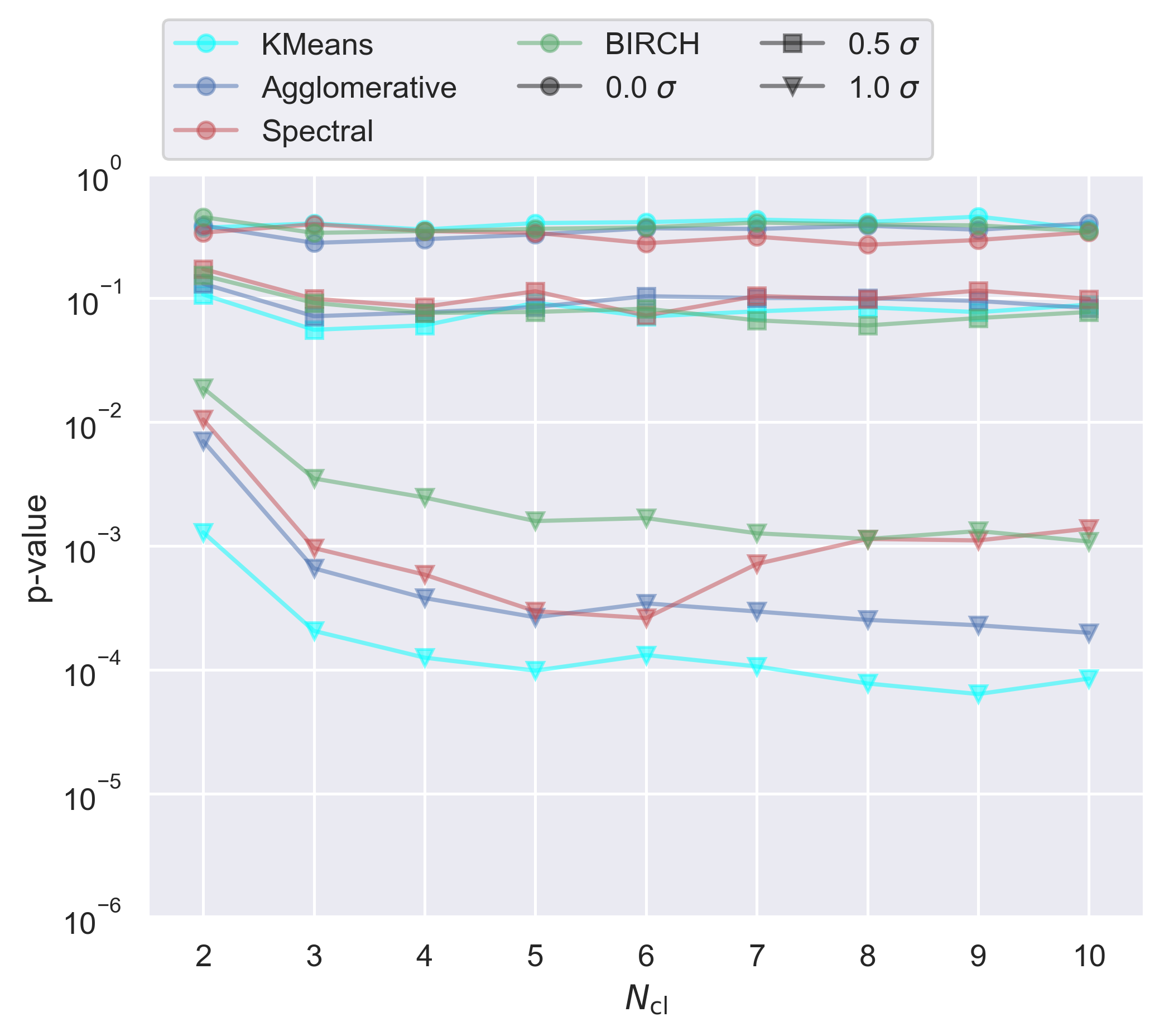
   Figure 1: p-value vs. number of clusters with different unsupervised clustering algorithms. There are three test cases: In case 1, we draw two subsets from two identical Gaussian distributions. In case 2 (3), we shift one of the Gaussian distributions by 0.5 (1.0) $\sigma$ before sampling the subsets. Subset 1 has 30 data points and subset 2 has 5570 data points, which is roughly the ratio of observed MW satellites to simulated satellites. The colours indicate different unsupervised clustering algorithms. The circles, squares, and triangles show results from case 1, 2 and 3 (0, 0.5, and 1.0 $\sigma$), respectively.

3.2 Clustering result and the p-value from our fiducial model

We show an example of the clustering result from our fiducial model in Fig. 2. All simulated galaxies from 30 Caterpillar trees are considered (the Ensemble). The data in each dimension is normalised before applying the Agglomerative clustering with 5 clusters. The clustering result is projected onto the $\langle\mathrm{[Fe/H]}\rangle$-${M_{*}}$ space and the mean values are shown in bold font. Galaxies that are assigned to different clusters are shown with different colours. The observed and the a-sloth simulated satellites are shown with squares and circles, respectively.

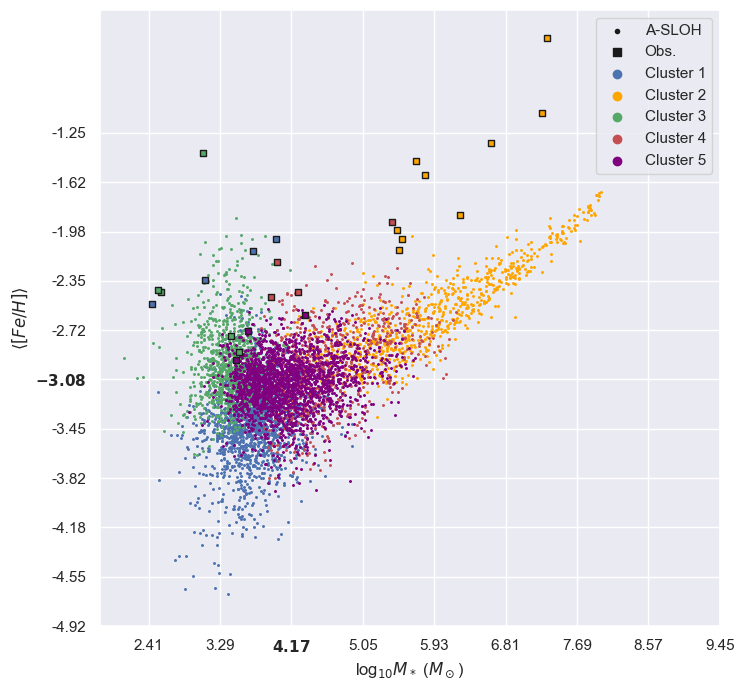
Figure 2: An example of unsupervised clustering from the fiducial model of a-sloth and the observed satellites, which is projected onto the $\langle\mathrm{[Fe/H]}\rangle$-${M_{*}}$ space. The data is normalised in each dimension before we apply the unsupervised clustering and the means are shown in bold font. In this analysis we use Agglomerative with 5 clusters. Galaxies that are classified in different clusters are plotted with different colours. Observed MW satellites are shown in squares and a-sloth simulated MW satellites are shown in circles. The p-value for this example is $10^{-2.2}$.

As mentioned in Sec. 2.2, we run the same analysis 100 times to take into account of the randomness in the solar position and obtain 100 p-values. We compute the geometric mean of the 100 p-values that we obtain with the Ensemble and take it as the final p-value for our fiducial model, which is $10^{-3.5\pm 1.4}$. In Fig. 3, we show the mean p-values with 1 standard deviation of 30 Caterpillar trees individually along with the p-value from the Ensemble. Even though the p-value from the Ensemble is low, we find that the p-values from individual Caterpillar trees span a wide range. This indicates that some Caterpillar trees are more similar to the MW than the others. For example, in one specific run for Tree H1631582, the algorithm finds two clusters that only consist of the simulated galaxies (Fig. 4), which leads to a p-value of $10^{-9.6}$. Further analysis of the merger histories of the individual Caterpillar trees with high p-values could potentially tell us more about the merger history of the MW.

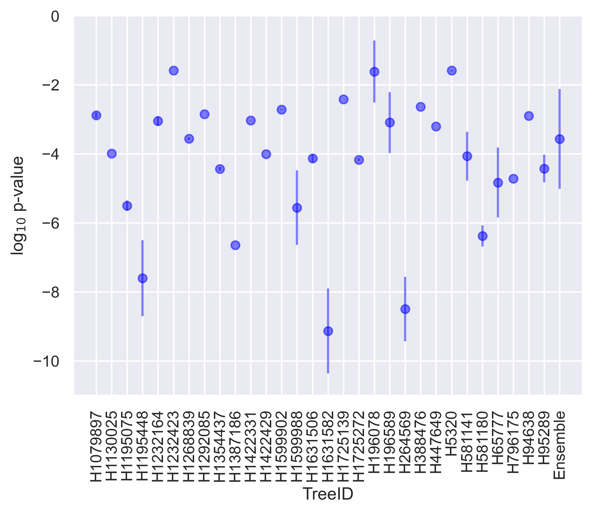
Figure 3: The p-values from 30 Caterpillar trees as individual datasets and the p-value from the Ensemble (data from 30 trees combined before conducting the analysis). Mean and 1 standard deviation from 100 runs of the analysis are shown with error bars.

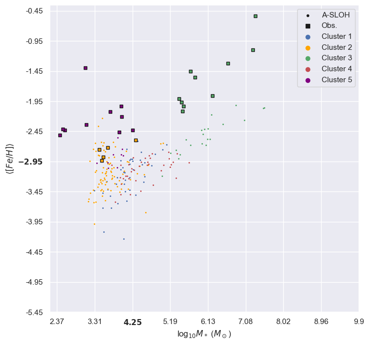
Figure 4: Similar to Fig. 2 but for one specific tree H1631582, which has the lowest p-value among the 30 Caterpillar trees. Two clusters only consist of simulated satellites and the p-value for this specific run is $10^{-9.6}$.

4 Discussion

4.1 Properties of the simulated MW satellites

In this section we discuss the reason why our fiducial model does not reproduce the observables of interest in more details. In Fig. 5 we show histograms of the five physical quantities that are used in our analysis from both the observed and a-sloth simulated satellites (fiducial and improved model). The biggest difference between the observed MW satellites and simulated galaxies from the fiducial model lies in the mean stellar [Fe/H], where we observe a difference of $\sim$ 1 dex. The overall distribution of the standard deviation of stellar [Fe/H] among the satellites is similar between the observed one and the fiducial model. There are a small number of simulated satellites that have scatter larger than 1 dex among the stars.

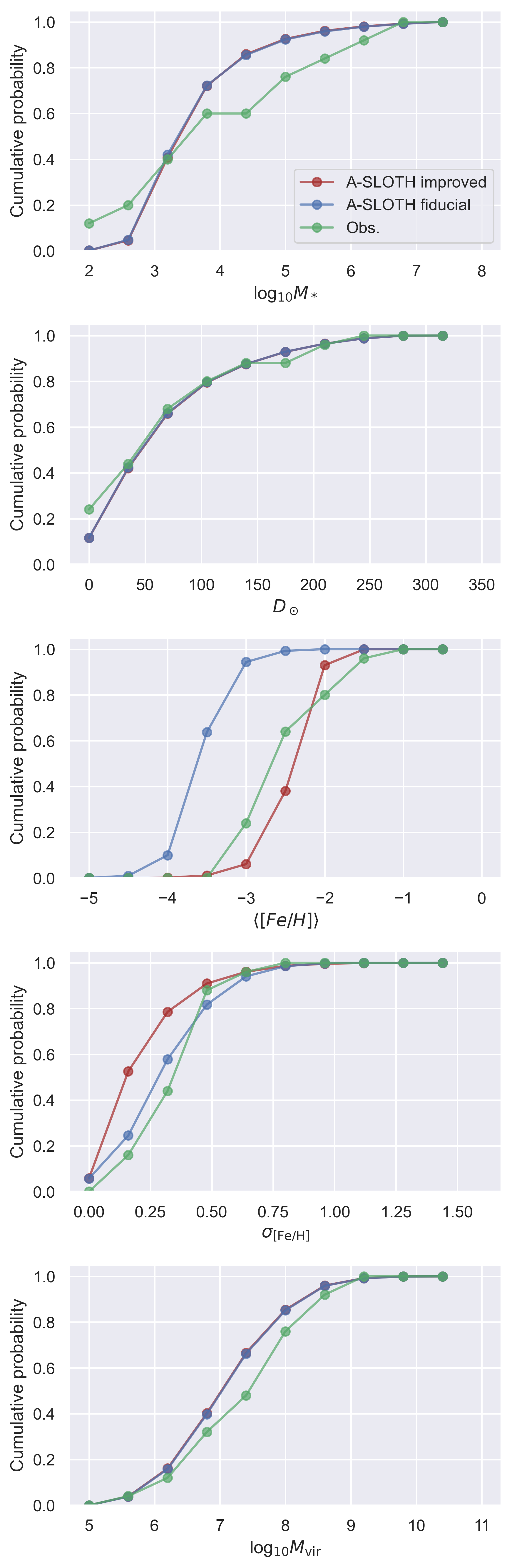
Figure 5: Normalised, cumulative histogram of the five physical quantities used in the analysis from our fiducial model, improved model, and the observation. From top to bottom: stellar mass, helicocentric distance, mean stellar $\mathrm{[Fe/H]}$, standard deviation of stellar $\mathrm{[Fe/H]}$, and the virial mass of the halo. The observation is plotted in green, the a-sloth fiducial model is plotted in blue, and the improved model is plotted in brown.

Here we define $N_{\mathrm{pass}}$ as the number of Caterpillar trees that have p-values > 0.01. We use it as an indicator of whether a-sloth is able to reproduce the observables. In addition to the visual inspection of Fig. 5, we re-run the analysis and exclude one physical quantity at a time to examine which one is most responsible for the inconsistency. The resulting $N_{\mathrm{pass}}$ is shown in Table 3. It is clear from this table that the mean stellar $\mathrm{[Fe/H]}$ is crucial. From the a-sloth fiducial model, $N_{\mathrm{pass}}=24$ if we exclude the mean stellar $\mathrm{[Fe/H]}$, whereas $N_{\mathrm{pass}}=0$ when we exclude any of the other four quantities.

Excluded quantity	$N_{\mathrm{pass,fid}}$	$N_{\mathrm{pass,imp}}$
$M_{*}$	0	10
$D_{\odot}$	0	4
$\langle\mathrm{[Fe/H]}\rangle$	24	24
$\sigma_{\mathrm{[Fe/H]}}$	0	3
$M_{\mathrm{vir}}$	0	2
All 5 quantities considered	3	6

Table 3: We run the same analysis but exclude one physical property at a time and show the number of Caterpillar trees that have p-values > 0.01 for the fiducial model and the improved model ($N_{\mathrm{pass,fid}}$ and $N_{\mathrm{pass,imp}}$). For comparison, we show $N_{\mathrm{pass}}$ from the fiducial and improved models if we consider all five physical quantities in the analysis.

In the fiducial model of a-sloth, we assume that the metals ejected from the halo mix with the inter-galactic medium (IGM) homogeneously and instantaneously, where we compute a mixing volume that is monotonically increasing over time. In reality, the metals expand outwards from the halo to the IGM. The newly injected metals should therefore stay in proximity to the halo, leading to a gradient in the radial metallicity profile of the IGM. Without exact spatial information of the gas, we are not able to model this radial profile properly. We here implement an ad-hoc solution where we assume that the re-accreted gas has a metallicity 8 times higher than the average IGM value.

$N_{\mathrm{pass}}$ increases from 3 to 6 as we improve the calculation of the IGM metallicity if we take all five physical quantities into account. From tests where we exclude one of the physical quantities, an increase of $N_{\mathrm{pass}}$ is shown except for when we exclude the mean stellar $\mathrm{[Fe/H]}$. This improvement of the model can also be observed in Fig. 5. However, we also find some of the Caterpillar trees actually have lower p-values from the improved model than from the fiducial one (Fig. 6). Despite the fact that the overall range of $\langle\mathrm{[Fe/H]}\rangle$ is now more similar between the observation and the improved model, the improved model still does not reproduce the cumulative distribution completely. This could explain why not all p-values from the 30 Caterpillar trees improve. Moreover, the new calculation of IGM metallicity also affects the metallicity distribution function of the MW, which is one of the observables that were used to calibrate the a-sloth model. We plan to further improve the metal mixing model in a future investigation.

To confirm that the above findings are independent of the p-value threshold, we test 4 additional cases where the p-value threshold = [0.003, 0.005, 0.03, 0.05]. We draw the same conclusion that mean stellar [Fe/H] is the property that our fiducial A-SLOTH model fails to reproduce. The improvement of the physical model is present regardless of the choice of p-value threshold. The number of Caterpillar trees that pass the threshold from these 4 tests are shown in Tables. 4-7.

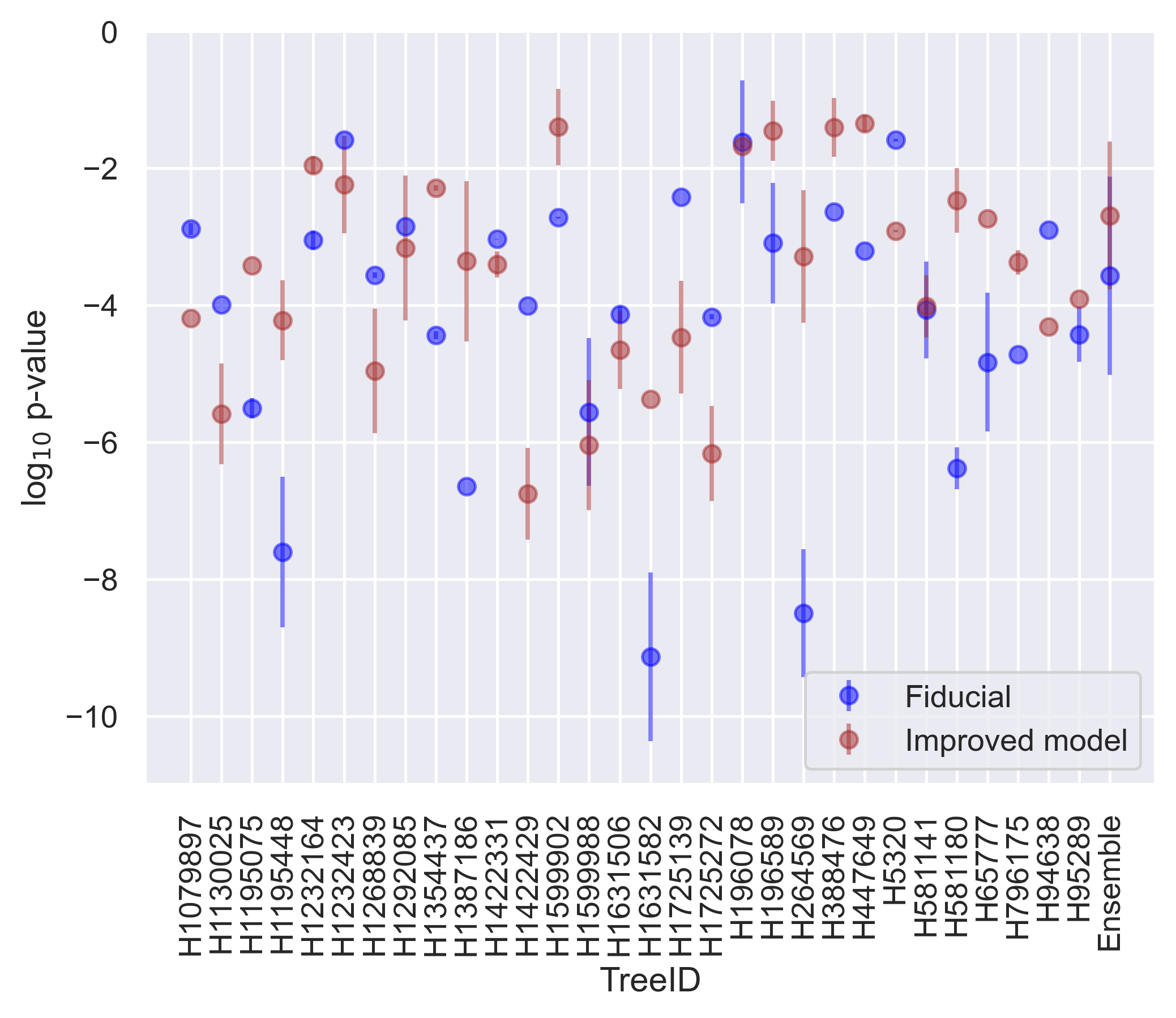
Figure 6: Similar to Fig. 3 but we add the p-values from the improved model in brown. The p-values from the fiducial model is shown in blue.

4.2 p-value vs. properties of the MW-like galaxies

As discussed in Sec. 3.2, the p-values from our 30 Caterpillar trees span a wide range. This is expected because our analysis involves information from the satellites, whereas the selection criteria for MW-like merger trees are only related with the main halo. In this section we further analyse the results regarding other properties of the dark matter merger trees to see if we can find consensus among the trees that have p-values larger than 0.01, below which we reject the null hypothesis that the tree is similar to the MW system. We show the p-values of individual Caterpillar trees from both the fiducial model and the improved one vs. some properties of the main galaxies (the MWs) in the trees: the virial mass of the halo at $z=0$, the stellar mass at $z=0$, number of satellites after applying the selection function, number of major halo growth ($\Delta M/M>30\%$), and the redshift of most recent major halo growth in Fig. 7. Compared to the trees that have p-values below the threshold, the virial mass of the main haloes are in a narrower range in trees that pass the threshold. We also find that these virial masses are at the upper limit of or higher than the observed MW virial mass (Posti & Helmi, 2019). For the other four properties, we find no distinct differences between the trees that pass the threshold and those that fail.

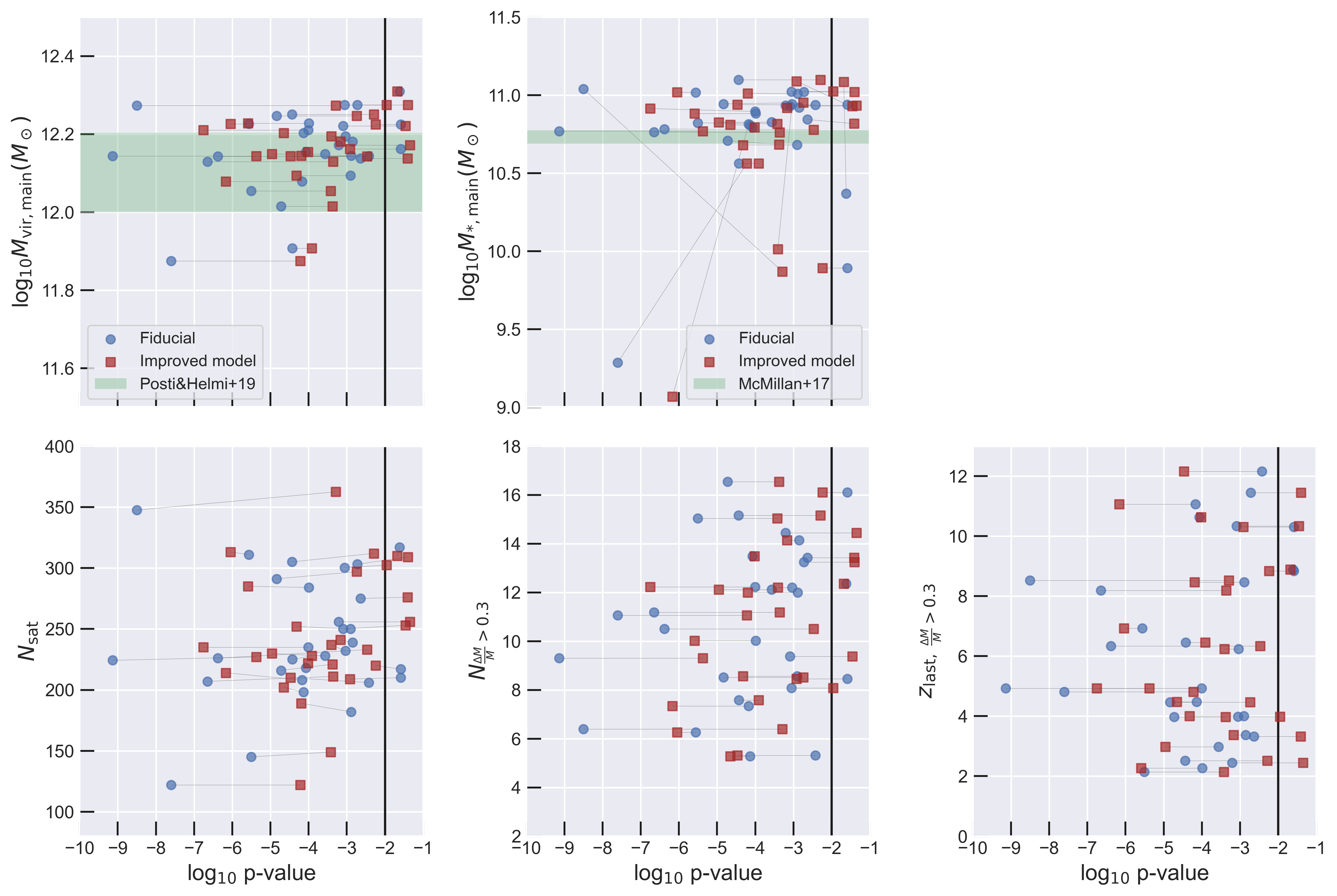
Figure 7: The p-values of individual Caterpillar trees vs. the properties of the main halo: the virial mass at $z=0$, the stellar mass at $z=0$, number of satellites (after applying the selection function), number of major halo growths ($\Delta M/M>30\%$), and the redshift of most recent major halo growth. Data from the fiducial model and the improved model are shown in blue and brown, respectively. The pairs of data points from the same trees are connected with thin black lines. The data is shifted slightly in the y-axis such that the pairs can be more easily identified. The observed MW stellar mass (McMillan, 2017) and virial mass (Posti & Helmi, 2019) are added with upper and lower limits in green bands.

4.3 Caveats

The stars listed in the SAGA database do not come from one survey or one group and may not be complete. As discussed in Suda et al. (2017), some stars are detected by different groups and may have different abundances in the literature. Values with the highest “priority parameter" are the fiducial values, which are the ones we take in our analysis. The resolving power, the publication year, whether ionisation state or molecules are used, the uncertainty, and the upper/lower limit are taken into account to determine the priority parameter. We also note that there are only 29 MW satellites listed in the SAGA database, while there are more than 50 MW satellites found (Muñoz et al., 2018). We aim to extend the study to individual stars in the dwarf satellites, therefore, the SAGA database is used. After applying the selection function, there are 25 observed MW satellites and an average of $>200$ MW satellites from the Caterpillar trees. This leads to the long-standing issue with the $\Lambda$CDM simulations, the “missing satellite problem" (Kauffmann et al., 1993; Moore et al., 1999; Klypin et al., 1999), which is beyond the scope of this analysis and the physical models in a-sloth.

5 Conclusion

In this work, we introduce a new analysis method that helps us analyse the results from the fiducial model of our semi-analytic code a-sloth. Unlike other earlier studies, we are able to calibrate the model with multiple observables in one go. The observed and simulated satellites are clustered in a 5-dimensional space using the unsupervised Agglomerative hierarchical clustering algorithm. We obtain a p-value based on the clustering result from the Fisher-Freeman-Halton exact test, which tells us whether the observed and simulated satellites come from the same underlying distribution.

We first test our method with two two-dimensional Gaussian distributions to compare results from different unsupervised clustering algorithms (KMeans, Agglomerative, Spectral, and BIRCH) and study the dependence on the number of clusters. KMeans is the most straightforward algorithm to use. However, one needs to presume the number of clusters and the pursuit of even sizes of clusters can lead to non-intuitive result. In contrary, the algorithm of Agglomerative hierarchical clustering does not depend on the number of clusters. It builds up a dendrogram and depending on the number of clusters requested, it returns the labelled data points based on the dendrogram. When the two Gaussian distributions are separated by $1\,\sigma$, we find sufficiently low p-values that allow us to reject the null hypothesis, which assumes that the two distributions come from the same underlying distribution. We observe a decrease in p-values when the number of clusters ($N_{\mathrm{cl}}$) increases. At $N_{\mathrm{cl}}\geq 5$, we start to observe converged p-values. Therefore, we adopt Agglomerative with 5 clusters as the fiducial values.

We then apply this method to the a-sloth simulated MW satellites and the observed ones. There are 5 physical quantities used in the analysis: the stellar mass $M_{*}$, the heliocentric distance $D_{\odot}$, the virial mass $M_{\mathrm{vir}}$, mean stellar metallicity $\langle\mathrm{[Fe/H]}\rangle$, and the scatter among the stellar metallicity $\sigma_{\mathrm{[Fe/H]}}$. The simulation is run with the fiducial model in the semi-analytic code a-sloth and we use 30 Caterpillar trees (Griffen et al., 2016). Due to the limitation of spatial information within the halo, we sample the solar position and run the analysis 100 times. The geometric mean of the 100 p-values is taken as the final p-value, which is $10^{-3.50\pm 1.42}$ from our fiducial a-sloth model. This tells us that the simulated MW satellites from our fiducial model do not come from the same underlying distribution of the observed ones, i.e., the physical model in a-sloth is not good enough.

We further analyse the simulated MW satellites and find that although the fiducial model in a-sloth is able to reproduce the stellar mass-to-halo mass relation at $z=0$ well, it is not able to reproduce the chemical properties of the observed MW satellites. We define $N_{\mathrm{pass}}$ as the number of Caterpillar trees that have p-values > 0.01, below which we reject the null hypothesis that the tree is similar to the MW system. Tests where we exclude one of the five quantities at a time indicate that the mean stellar $\mathrm{[Fe/H]}$ is the main quantity that a-sloth fails to reproduce (Table 3). In Fig. 5, we find that most of the a-sloth simulated satellites have stellar $\mathrm{[Fe/H]}$ almost 1 dex lower than the observed ones. This can be partly explained by the simplified assumption of homogeneous and instantaneous mixing when we determine the matallicity of the re-accreted IGM. We implement an ad-hoc model that assumes the IGM metallicity is higher in the proximity to the halo and the metallicity of the accreted gas is 8 times the mean IGM value. The goal of this paper is to introduce the new analysis method and we will further improve the chemical model in a-sloth in future works.

To understand why some of the Caterpillar trees pass the $p=0.01$ threshold while the others don’t, we further compare the p-values from individual trees with the properties of their main haloes: the virial mass at $z=0$, the stellar mass at $z=0$, the number of satellites after applying the selection function, number of major halo growths ($\Delta M/M>30\%$), and the redshift of most recent major halo growth. Among the trees that pass the threshold, the virial masses of their main halo are in a narrow range [$10^{12.1}{\rm M}_{\odot}-10^{12.3}{\rm M}_{\odot}$]. For the other properties, there are no distinct differences between the trees that pass the threshold and those that fail.

This new method of comparing observational and simulated data in high-dimensional space can distinguish a good model from a bad one easily. It has no limitation on the data size or how the data distribution looks like. We aim to further improve the physical model in a-sloth and continue using this method. More importantly, we plan to consider stellar information such as [C/Fe], [Ba/Fe], [Eu/Fe], etc, to study the elemental abundances of individual stars of the MW satellites in our future works.

Software

a-sloth (Magg et al., 2022), matplotlib (Hunter, 2007), numpy (Harris et al., 2020), pandas (Wes McKinney, 2010; Reback et al., 2022), python (Van Rossum & Drake, 2009), Scikit-learn (Pedregosa et al., 2011), scipy (Virtanen et al., 2020), stats in R (R Core Team, 2013; R Core Team, 2021).

DATA AVAILABILITY

The observational data used in this work can be found in the references listed in the main text. The simulated data and analysis results underlying this article will be shared on reasonable request to the corresponding author. a-sloth is publicly available at https://gitlab.com/thartwig/asloth and the analysis script used in this work can be found at https://gitlab.com/thartwig/asloth/-/tree/main/scripts/p-value.

Appendix A Number of trees that pass the p-value threshold vs. different thresholds

The p-value threshold of 0.01 that we use in the analysis is a conventional choice (Sec. 4.1). To examine the dependence of our results on this threshold, we test additionally 4 different values (0.003, 0.005, 0.03, and 0.05). We show how many Caterpillar trees pass the threshold from these tests in Tables 4-7. We find a consensus among the tests that mean stellar $\mathrm{[Fe/H]}$ is the property which the fiducial a-sloth model fails to reproduce. Our modified model produces improved results in all tests, independent of the p-value threshold.

Excluded quantity	$N_{\mathrm{pass,fid}}$	$N_{\mathrm{pass,imp}}$
$M_{*}$	1	18
$D_{\odot}$	1	8
$\langle\mathrm{[Fe/H]}\rangle$	29	27
$\sigma_{\mathrm{[Fe/H]}}$	0	7
$M_{\mathrm{vir}}$	0	8
All 5 quantities considered	4	9

Table 4: Similar to Table 3 but with p-value threshold = 0.003.

Excluded quantity	$N_{\mathrm{pass,fid}}$	$N_{\mathrm{pass,imp}}$
$M_{*}$	0	13
$D_{\odot}$	0	6
$\langle\mathrm{[Fe/H]}\rangle$	27	27
$\sigma_{\mathrm{[Fe/H]}}$	0	6
$M_{\mathrm{vir}}$	0	5
All 5 quantities considered	3	8

Table 5: Similar to Table 3 but with p-value threshold = 0.005.

Excluded quantity	$N_{\mathrm{pass,fid}}$	$N_{\mathrm{pass,imp}}$
$M_{*}$	0	5
$D_{\odot}$	0	3
$\langle\mathrm{[Fe/H]}\rangle$	23	17
$\sigma_{\mathrm{[Fe/H]}}$	0	2
$M_{\mathrm{vir}}$	0	2
All 5 quantities considered	0	4

Table 6: Similar to Table 3 but with p-value threshold = 0.03.

Excluded quantity	$N_{\mathrm{pass,fid}}$	$N_{\mathrm{pass,imp}}$
$M_{*}$	0	3
$D_{\odot}$	0	3
$\langle\mathrm{[Fe/H]}\rangle$	17	16
$\sigma_{\mathrm{[Fe/H]}}$	0	2
$M_{\mathrm{vir}}$	0	2
All 5 quantities considered	0	0

Table 7: Similar to Table 3 but with p-value threshold = 0.05.

References

- Battaglia & Nipoti (2022) Battaglia G., Nipoti C., 2022, Nature Astronomy, 6, 659
- Battaglia et al. (2022) Battaglia G., Taibi S., Thomas G. F., Fritz T. K., 2022, A&A, 657, A54
- Belokurov et al. (2010) Belokurov V., et al., 2010, ApJ, 712, L103
- Chen et al. (2022) Chen L.-H., Magg M., Hartwig T., Glover S. C. O., Ji A. P., Klessen R. S., 2022, MNRAS, 513, 934
- Chiti et al. (2018) Chiti A., Frebel A., Ji A. P., Jerjen H., Kim D., Norris J. E., 2018, ApJ, 857, 74
- Chiti et al. (2021) Chiti A., et al., 2021, Nature Astronomy, 5, 392
- Chiti et al. (2022) Chiti A., et al., 2022, arXiv e-prints, p. arXiv:2205.01740
- Drlica-Wagner et al. (2015) Drlica-Wagner A., et al., 2015, ApJ, 813, 109
- Errani et al. (2018) Errani R., Peñarrubia J., Walker M. G., 2018, MNRAS, 481, 5073
- Fasano & Franceschini (1987) Fasano G., Franceschini A., 1987, MNRAS, 225, 155
- Fisher (1934) Fisher R. A., 1934, Statistical Methods for Research Workers, Fifth Edision. Oliver and Boyd, Edingburgh
- Font et al. (2011) Font A. S., et al., 2011, MNRAS, 417, 1260
- Freeman & Halton (1951) Freeman G. H., Halton J. H., 1951, Biometrika, 38, 141
- Gallart et al. (2021) Gallart C., et al., 2021, ApJ, 909, 192
- Garcia-Dias et al. (2018) Garcia-Dias R., Allende Prieto C., Sánchez Almeida J., Ordovás-Pascual I., 2018, A&A, 612, A98
- Griffen et al. (2016) Griffen B. F., Ji A. P., Dooley G. A., Gómez F. A., Vogelsberger M., O’Shea B. W., Frebel A., 2016, ApJ, 818, 10
- Harris et al. (2020) Harris C. R., et al., 2020, Nature, 585, 357
- Hartwig et al. (2015) Hartwig T., Bromm V., Klessen R. S., Glover S. C. O., 2015, MNRAS, 447, 3892
- Hartwig et al. (2022) Hartwig T., et al., 2022, ApJ, 936, 45
- Hunter (2007) Hunter J. D., 2007, Computing in Science & Engineering, 9, 90
- Jeon et al. (2017) Jeon M., Besla G., Bromm V., 2017, ApJ, 848, 85
- Ji et al. (2016) Ji A. P., Frebel A., Chiti A., Simon J. D., 2016, Nature, 531, 610
- Ji et al. (2021) Ji A. P., et al., 2021, ApJ, 921, 32
- Kang et al. (2022) Kang D. E., Pellegrini E. W., Ardizzone L., Klessen R. S., Koethe U., Glover S. C. O., Ksoll V. F., 2022, MNRAS, 512, 617
- Kauffmann et al. (1993) Kauffmann G., White S. D. M., Guiderdoni B., 1993, MNRAS, 264, 201
- Kirby et al. (2017) Kirby E. N., Cohen J. G., Simon J. D., Guhathakurta P., Thygesen A. O., Duggan G. E., 2017, ApJ, 838, 83
- Klypin et al. (1999) Klypin A., Gottlöber S., Kravtsov A. V., Khokhlov A. M., 1999, ApJ, 516, 530
- Kolmogorov (1933) Kolmogorov A. N., 1933, Giornale dell’Istituto Italiano degli Attuari, 4, 83
- Koposov et al. (2009) Koposov S. E., Yoo J., Rix H.-W., Weinberg D. H., Macciò A. V., Escudé J. M., 2009, ApJ, 696, 2179
- Koposov et al. (2015) Koposov S. E., Belokurov V., Torrealba G., Evans N. W., 2015, ApJ, 805, 130
- Ksoll et al. (2021a) Ksoll V. F., et al., 2021a, AJ, 161, 256
- Ksoll et al. (2021b) Ksoll V. F., et al., 2021b, AJ, 161, 257
- Logan & Fotopoulou (2020) Logan C. H. A., Fotopoulou S., 2020, A&A, 633, A154
- Magg et al. (2016) Magg M., Hartwig T., Glover S. C. O., Klessen R. S., Whalen D. J., 2016, MNRAS, 462, 3591
- Magg et al. (2022) Magg M., Hartwig T., Chen L.-H., Tarumi Y., 2022, The Journal of Open Source Software, 7, 4417
- McConnachie (2012) McConnachie A. W., 2012, AJ, 144, 4
- McConnachie & Venn (2020) McConnachie A. W., Venn K. A., 2020, AJ, 160, 124
- McMillan (2017) McMillan P. J., 2017, MNRAS, 465, 76
- Moore et al. (1999) Moore B., Ghigna S., Governato F., Lake G., Quinn T., Stadel J., Tozzi P., 1999, ApJ, 524, L19
- Muñoz et al. (2006) Muñoz R. R., Carlin J. L., Frinchaboy P. M., Nidever D. L., Majewski S. R., Patterson R. J., 2006, ApJ, 650, L51
- Muñoz et al. (2018) Muñoz R. R., Côté P., Santana F. A., Geha M., Simon J. D., Oyarzún G. A., Stetson P. B., Djorgovski S. G., 2018, ApJ, 860, 66
- Peacock (1983) Peacock J. A., 1983, MNRAS, 202, 615
- Pearson (1916) Pearson K., 1916, Philosophical Transactions of the Royal Society of London Series A, 216, 429
- Pedregosa et al. (2011) Pedregosa F., et al., 2011, Journal of Machine Learning Research, 12, 2825
- Posti & Helmi (2019) Posti L., Helmi A., 2019, A&A, 621, A56
- R Core Team (2013) R Core Team 2013, R: A Language and Environment for Statistical Computing. R Foundation for Statistical Computing, Vienna, Austria, %****␣ml.bbl␣Line␣275␣****http://www.R-project.org/
- R Core Team (2021) R Core Team 2021, R: A Language and Environment for Statistical Computing. R Foundation for Statistical Computing, Vienna, Austria, https://www.R-project.org/
- Reback et al. (2022) Reback J., et al., 2022, pandas-dev/pandas: Pandas 1.4.1, doi:10.5281/zenodo.6053272.
- Reichert et al. (2020) Reichert M., Hansen C. J., Hanke M., Skúladóttir Á., Arcones A., Grebel E. K., 2020, A&A, 641, A127
- Reis et al. (2019) Reis I., Rotman M., Poznanski D., Prochaska J. X., Wolf L., 2019, arXiv e-prints, p. arXiv:1911.06823
- Ricotti & Gnedin (2005) Ricotti M., Gnedin N. Y., 2005, ApJ, 629, 259
- Rolleston et al. (2003) Rolleston W. R. J., Venn K., Tolstoy E., Dufton P. L., 2003, A&A, 400, 21
- Romano et al. (2019) Romano D., Calura F., D’Ercole A., Few C. G., 2019, A&A, 630, A140
- Safarzadeh & Scannapieco (2017) Safarzadeh M., Scannapieco E., 2017, MNRAS, 471, 2088
- Salvadori et al. (2015) Salvadori S., Skúladóttir Á., Tolstoy E., 2015, MNRAS, 454, 1320
- Sanati et al. (2022) Sanati M., Jeanquartier F., Revaz Y., Jablonka P., 2022, arXiv e-prints, p. arXiv:2206.11351
- Simon (2019) Simon J. D., 2019, ARA&A, 57, 375
- Starkenburg et al. (2013) Starkenburg E., et al., 2013, MNRAS, 429, 725
- Suda et al. (2008) Suda T., et al., 2008, PASJ, 60, 1159
- Suda et al. (2017) Suda T., et al., 2017, PASJ, 69, 76
- Tarumi et al. (2020) Tarumi Y., Hartwig T., Magg M., 2020, ApJ, 897, 58
- Tsujimoto et al. (1995) Tsujimoto T., Nomoto K., Yoshii Y., Hashimoto M., Yanagida S., Thielemann F. K., 1995, MNRAS, 277, 945
- Van Rossum & Drake (2009) Van Rossum G., Drake F. L., 2009, Python 3 Reference Manual. CreateSpace, Scotts Valley, CA
- Van der Swaelmen et al. (2013) Van der Swaelmen M., Hill V., Primas F., Cole A. A., 2013, A&A, 560, A44
- Virtanen et al. (2020) Virtanen P., et al., 2020, Nature Methods, 17, 261
- Walker et al. (2007) Walker M. G., Mateo M., Olszewski E. W., Gnedin O. Y., Wang X., Sen B., Woodroofe M., 2007, ApJ, 667, L53
- Wang et al. (2021) Wang W., et al., 2021, MNRAS, 500, 3776
- Wang et al. (2022) Wang G.-J., Shi H.-L., Yan Y.-P., Xia J.-Q., Zhao Y.-Y., Li S.-Y., Li J.-F., 2022, ApJS, 260, 13
- Weisz et al. (2014) Weisz D. R., Dolphin A. E., Skillman E. D., Holtzman J., Gilbert K. M., Dalcanton J. J., Williams B. F., 2014, ApJ, 789, 148
- Wes McKinney (2010) Wes McKinney 2010, in Stéfan van der Walt Jarrod Millman eds, Proceedings of the 9th Python in Science Conference. pp 56 – 61, doi:10.25080/Majora-92bf1922-00a
- Wheeler et al. (2019) Wheeler C., et al., 2019, MNRAS, 490, 4447
- Yoon et al. (2020) Yoon J., Whitten D. D., Beers T. C., Lee Y. S., Masseron T., Placco V. M., 2020, ApJ, 894, 7