Absence of entanglement transition due to feedback-induced skin effect

Abstract

A quantum many-body system subject to unitary evolution and repeated local measurements with an increasing rate undergoes an entanglement transition from extensive (or subextensive) to area law entropy scaling. We find that certain open boundary systems under “generalized monitoring”, consisting of “projective monitoring” and conditional feedback, display an anomalous late-time particle concentration on the edge, reminiscent of the “skin effect” in non-Hermitian systems. Such feedback-induced skin effect will suppress the entanglement generation, rendering the system short-range entangled without any entanglement transition. While initially emerged in non-interacting models, such skin effect can also occur in chaotic interacting systems and Floquet quantum circuits subjected to random generalized measurements. Since the dynamics of skin-effect do not require post-selection, and can be observed at the particle number level, the phenomenon is experimentally relevant and accessible in noisy intermediate-scale quantum platforms, such as trapped ions.

1 Introduction

The competition between the measurement and unitary evolution produces a novel measurement-induced phase transition (MIPT) [Li et al.(2018)Li, Chen, and Fisher, Skinner et al.(2019)Skinner, Ruhman, and Nahum, Chan et al.(2019)Chan, Nandkishore, Pretko, and Smith, Li et al.(2019)Li, Chen, and Fisher, Fidkowski et al.(2021)Fidkowski, Haah, and Hastings, Nahum et al.(2021)Nahum, Roy, Skinner, and Ruhman, Ippoliti et al.(2021a)Ippoliti, Gullans, Gopalakrishnan, Huse, and Khemani, Fisher et al.(2022a)Fisher, Khemani, Nahum, and Vijay, Li et al.(2021a)Li, Chen, Ludwig, and Fisher, Chen et al.(2020)Chen, Li, Fisher, and Lucas, Zabalo et al.(2020)Zabalo, Gullans, Wilson, Gopalakrishnan, Huse, and Pixley], where a random quantum circuit [Chan et al.(2018)Chan, De Luca, and Chalker, Nahum et al.(2018)Nahum, Vijay, and Haah, von Keyserlingk et al.(2018)von Keyserlingk, Rakovszky, Pollmann, and Sondhi, Zhou and Nahum(2019), Fisher et al.(2022b)Fisher, Khemani, Nahum, and Vijay] interspersed by onsite measurements with an increasing rate goes from a volume-law regime to an area-law regime. Similar entanglement transitions also appear in the context of monitored fermions [Alberton et al.(2021)Alberton, Buchhold, and Diehl, Cao et al.(2019)Cao, Tilloy, and Luca, Coppola et al.(2022)Coppola, Tirrito, Karevski, and Collura, Carollo and Alba(2022), Turkeshi et al.(2021)Turkeshi, Biella, Fazio, Dalmonte, and Schiró, Biella and Schiró(2021), Müller et al.(2022)Müller, Diehl, and Buchhold, Minato et al.(2022)Minato, Sugimoto, Kuwahara, and Saito, Buchhold et al.(2021)Buchhold, Minoguchi, Altland, and Diehl], monitored open systems [Ladewig et al.(2022)Ladewig, Diehl, and Buchhold, Turkeshi et al.(2022b)Turkeshi, Piroli, and Schiró], circuits with pure measurements [Lavasani et al.(2021)Lavasani, Alavirad, and Barkeshli, Ippoliti et al.(2021b)Ippoliti, Gullans, Gopalakrishnan, Huse, and Khemani], random tensor networks [Vasseur et al.(2019)Vasseur, Potter, You, and Ludwig, Lopez-Piqueres et al.(2020)Lopez-Piqueres, Ware, and Vasseur, Jian et al.(2022)Jian, Bauer, Keselman, and Ludwig, Yang et al.(2022)Yang, Li, Fisher, and Chen], and quantum error correction thresholds [Choi et al.(2020)Choi, Bao, Qi, and Altman, Gullans and Huse(2020a), Gullans and Huse(2020b), Gullans et al.(2021)Gullans, Krastanov, Huse, Jiang, and Flammia]. Measurements introduce intrinsic randomness to the otherwise deterministic dynamics, with each set of recorded measurement results corresponding to a specific trajectory [Daley(2014)]. Among various frameworks trying to explain the MIPT [Bao et al.(2020)Bao, Choi, and Altman, Jian et al.(2020)Jian, You, Vasseur, and Ludwig, Li and Fisher(2021), Li et al.(2021b)Li, Vasseur, Fisher, and Ludwig, Buchhold et al.(2021)Buchhold, Minoguchi, Altland, and Diehl, Choi et al.(2020)Choi, Bao, Qi, and Altman, Gullans and Huse(2020a), Gullans and Huse(2020b), Gullans et al.(2021)Gullans, Krastanov, Huse, Jiang, and Flammia, Cao et al.(2019)Cao, Tilloy, and Luca, Turkeshi et al.(2022a)Turkeshi, Dalmonte, Fazio, and Schirò, Ippoliti and Khemani(2021), Ippoliti et al.(2022)Ippoliti, Rakovszky, and Khemani, Iadecola et al.(2022)Iadecola, Ganeshan, Pixley, and Wilson], one approach focuses on a specific trajectory, of which the evolution is described by a non-Hermitian Hamiltonian, where the entanglement transition in some systems coincides with the spontaneous $PT$ symmetry breaking [Kells et al.(2023)Kells, Meidan, and Romito, Turkeshi and Schiró(2023), Jian et al.(2021)Jian, Yang, Bi, and Chen, Kawabata et al.(2022)Kawabata, Numasawa, and Ryu, Gopalakrishnan and Gullans(2021)].

One unique phenomenon in certain non-Hermitian open boundary systems is the non-Hermitian skin effect [Yao and Wang(2018), Martinez Alvarez et al.(2018)Martinez Alvarez, Barrios Vargas, and Foa Torres, Zhang et al.(2020)Zhang, Yang, and Fang, Yokomizo and Murakami(2019), Okuma et al.(2020)Okuma, Kawabata, Shiozaki, and Sato, Yang et al.(2020)Yang, Zhang, Fang, and Hu, Yang et al.(2020)Yang, Zhang, Fang, and Hu, Borgnia et al.(2020)Borgnia, Kruchkov, and Slager, Torres(2019)], where a finite portion of the eigenstates are spatially concentrated on the edges. Dynamically, the skin effect implies that the late-time state from the quench dynamics will have particles concentrated near the edges. The Pauli exclusion principle predicts a nearly tensor-product structure of the steady state which obeys the area-law entanglement scaling, suggesting the absence of MIPT and seemingly contradicting the putative universal entanglement transition in the monitored systems. However, this simple argument assumes that the particular non-Hermitian evolution captures the entanglement behavior of the whole ensemble of trajectories, which is generally not guaranteed. Indeed, we will show in this work that under “projective monitoring” (the exact definition of which will be given later), on the trajectory ensemble level, there will be no skin effect.

A natural question is whether the skin effect can appear in the whole ensemble of trajectories and thus suppress the entanglement transition. In this work, we answer the question positively by considering a generalized version of monitoring, which contains conditional unitary feedback following projective monitoring. In certain generalized monitored systems, there is a dynamical skin effect induced by the feedback, which we called the feedback-induced skin effect (FISE). We introduce an extensive local order parameter, the classical entropy $S_{\text{cl}}$, which not only characterizes the skin effect but also imposes an upper bound on the bipartite entanglement entropy, i.e., $S_{\text{cl}}>2S_{A}$, where $S_{A}$ is the bipartite entanglement entropy for any subsystem $A$. Numerical simulations of finite-size open boundary systems show a scale invariance of the steady-state classical entropy:

$$S_{\mathrm{cl}}(\gamma,L)=L\cdot G(\gamma L^{1/\nu}),\quad G(x\rightarrow\infty)\sim c/x^{\nu},$$ (1)

which implies the saturation of the entanglement entropy in the thermodynamics limit at arbitrarily small measurement rates. That is, for vanishing small $\gamma$, the scaling form in Eq. (1) implies $S_{A}<c/\gamma^{\nu}$, which is a large but constant value (does not scale with system size) and therefore the system is in the area-law entangled phase. Remarkably, Eq. (1) persists even when the interaction is turned on, therefore eliminating (sub)extensive entangled phases believed to appear in the weakly-monitored regime.

Besides the continuous monitoring, FISE also appears in the randomly measured Floquet circuits, where the unitary evolution has only discrete spatial-temporal translation symmetry, and the monitoring process is the conventional projective measurement followed by a feedback operation. Such quantum circuit models provide a novel type of dynamical skin effect, which is essentially a many-body phenomenon not described by any Hamiltonian. The quantum circuit model is also experimentally relevant to the noisy intermediate-scale quantum devices. As we will show in this work, the establishing of the localized steady state from a “domain-wall state” only takes constant time, and only require a moderate system size to achieve it. We propose to implement such dynamical skin effect on the trapped-ion platforms.

The structure of this paper is as follows. In Sec. 2, we analyze why projective monitoring dynamics fail to produce the desired particle accumulation and explain how the introduction of conditional feedback enables the dynamical skin effect. In Sec. 3, we investigate the phenomenologies of the feedback-induced skin effect and explore its influence on the measurement-induced entanglement transition. In Sec. 4, we extend the study of the feedback-induced skin effect to quantum circuit models with discrete spatial and temporal translation symmetry under random generalized measurements. Finally, we conclude our work in Sec. 5.

2 Monitoring dynamics

2.1 Projective monitoring

A standard quantum measurement process can be represented by a set of projectors ${P_{m}}$, each corresponding to a different measurement outcome. Measuring a state $|\psi\rangle$ yields a probability distribution over the possible outcomes, given by the Born rule: $p_{m}=\langle\psi|P_{m}|\psi\rangle$. The state then collapses to $P_{m}|\psi\rangle/\sqrt{p_{m}}$. When the unitary evolution is governed by a Hamiltonian, we can consider a coarse-grained version of the dynamics known as projective monitoring. This approach is formulated using the stochastic Schrödinger equation (SSE) [Jacobs and Steck(2006), Wiseman and Milburn(2009), Barchielli and Gregoratti(2009)]:

$$d|\psi\rangle= \ -i\left[H-\frac{i\gamma}{2}\sum_{m}(P_{m}-\langle\psi|P_{m}|\psi\rangle)\right]|\psi\rangle dt+\sum_{m}\left[\frac{P_{m}|\psi\rangle}{\|P_{m}|\psi\rangle\|}-|\psi\rangle\right]dW_{m},$$ (2)

where each $dW_{m}$ is an independent Poisson random variable taking the values 0 or 1. In a small time interval $\Delta t$, the probability of observing $dW_{m}=1$ (i.e., the probe registers a quantum jump) is proportional to $\gamma\Delta t$. If $dW_{m}=0$ for all $m$ (the no-click limit) [Wiseman and Milburn(2009), Daley(2014)], the evolution is described by an effective non-Hermitian Hamiltonian

$$H_{\text{eff}}=H-i\frac{\gamma}{2}\sum_{m}P_{m}.$$ (3)

However, the no-click limit requires exponentially many experiments to be carried out before a desired trajectory is obtained.

In this section, we first consider a spinless fermion chain described by a nearest-neighbor hopping Hamiltonian:

$$H=\sum_{i}(c_{i}^{\dagger}c_{i+1}+c_{i+1}^{\dagger}c_{i}).$$ (4)

The observable of interest in this system is the occupation number of a local quasimode created by a two-site projector $P_{i}=d_{i}^{\dagger}d_{i}$, where $d_{i}=\frac{1}{\sqrt{2}}(c_{i}+ic_{i+1})$. The effective non-Hermitian Hamiltonian (3) for the monitored system is given by

$$H_{\mathrm{eff}}=\sum_{i}\left[\left(1+\frac{\gamma}{4}\right)c_{i}^{\dagger}c_{i+1}+\left(1-\frac{\gamma}{4}\right)c_{i+1}^{\dagger}c_{i}-i\frac{\gamma}{4}(n_{i}+n_{i+1})\right].$$ (5)

This Hamiltonian is known as the Hatano-Nelson model [Hatano and Nelson(1996)] and displays the non-Hermitian skin effect. Consider the evolution of the “domain-wall” state:

$$|\psi_{0}\rangle\equiv|1\cdots 10\cdots 0\rangle.$$ (6)

In the no-click limit and under open boundary conditions, the effective non-Hermitian Hamiltonian (5) results in a late-time particle accumulation on the left edge (as displayed on the left panel of Fig. 1). On the contrary, in the projective monitoring case, the detected right-moving quasimodes will balance out the momentum distribution, leaving a steady state of homogeneity (as displayed on the right panel of Fig. 1).

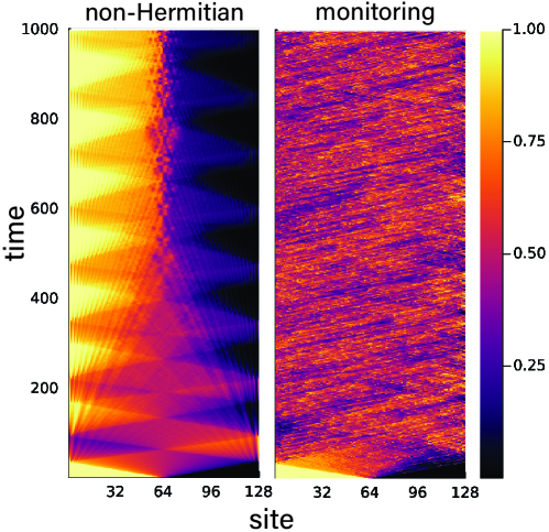
Figure 1: Comparison of non-Hermitian and monitoring dynamics starting from the initial state (6) and under open boundary conditions. Left panel: density evolution under non-Hermitian Hamiltonian with $\gamma=0.1$, where the particles gradually concentrate on the left. Right panel: density evolution under projective monitoring with $\gamma=0.1$ (for a single set of measurement results). Although monitoring creates random quantum jump processes and thus introduces density fluctuation, the density distribution on a large scale is homogeneous.

Besides SSE, the trajectory-averaged dynamics can also be formulated as the Lindblad master equation [Lindblad(1976), Davies(1974), Breuer and Petruccione(2007)]:

$$\frac{d}{dt}\rho=-i[H,\rho]-\frac{\gamma}{2}\sum_{m}\{L_{m}^{\dagger}L_{m},\rho\}+\gamma\sum_{m}L_{m}\rho L_{m}^{\dagger},$$ (7)

where $\overline{|\psi\rangle\langle\psi|}$ is the density matrix averaged over all trajectories, and $L_{m}=P_{m}$ is referred to as the jump operator. A state $\rho_{\mathrm{NESS}}$ is a nonequilibrium steady state (NESS) if $\partial_{t}\rho_{\mathrm{NESS}}=0$. Note that for the projective monitored dynamics, all jump operators $\{P_{i}\}$ are Hermitian. The maximally mixed state within a given particle-number sector $\rho=(\operatorname{Tr}\mathbb{I}_{\nu})^{-1}{\mathbb{I}}_{\nu}$ (the subscript indicates the subspace spanned by the states of filling number $\nu$) is automatically a steady state since

$$\frac{d}{dt}{\mathbb{I}}_{\nu} =-\frac{\gamma}{2}\sum_{m}\{P_{m},{\mathbb{I}}_{\nu}\}+\gamma\sum_{m}P_{m}{\mathbb{I}}_{\nu}P_{m}^{\dagger}$$ (8)

$$=-\gamma\sum_{m}\left.P_{m}\right|_{\nu}+\gamma\sum_{m}\left.P_{m}\right|_{\nu}=0.$$

In addition, $\rho_{\mathrm{NESS}}$ for generic Lindblad equation is nondegenerate (within each symmetry sector) [Evans(1977), Frigerio(1978), Spohn(1980), Prosen(2015)]. In Refs. [Evans(1977), Frigerio(1978)] (see review in Ref. [Spohn(1980)] and application in Ref. [Prosen(2015)], where the system is under boundary driven [Berdanier et al.(2019)Berdanier, Marino, and Altman]), it was shown that a Lindblad equation has unique nonequilibrium steady state if and only if the set

$$\mathcal{O}\equiv\{H,L_{1},L_{1}^{\dagger},L_{2},L_{2}^{\dagger},\cdots\}$$ (9)

generates (under multiplication and addition) the complete algebra on the Hilbert space. We prove the uniqueness of the steady state $\rho_{\mathrm{NESS}}$ for the specific model considered in this work in Appendix A. In conclusion, in the projective monitoring case, we expect no skin-effect-like dynamics.

2.2 Gemeralized monitoring

It is important to note that projective monitoring is an idealized representation of an actual measurement process. In practice, detecting a quantum state requires a probe to interact with the system, which inevitably disturbs the measured states. The more general form of a quantum measurement is described by the positive operator-valued measure (POVM) formalism [Nielsen and Chuang(2010), Wilde(2013)]. A continuous version of the POVM, called the generalized monitoring, is formulated as the stochastic Schrödinger equation (SSE) in Eq.(2), with the projector $P_{m}$ replaced by a general operator $L_{m}$ (see Appendix B.1 for a short review). In this study, we focus on a particular form of SSE where

$$L_{m}=U_{m}P_{m},$$ (10)

corresponding to adding a unitary feedback operator $U_{m}$ to the projective monitoring process. The conditional feedback does not affect the effective non-Hermitian Hamiltonian $H_{\mathrm{eff}}$, but instead operates on those trajectories that deviated from the post-selected trajectory.

Consider a conditional unitary operator

$$U_{i}=\exp(i\theta n_{i+1})$$ (11)

acting on sites ($i,i+1$) whenever the probe detect a right moving mode $d^{\dagger}d$. We temporarily fix $\theta=\pi$ so that the feedback $U_{i}$ converts the detected right-moving mode to a left-moving mode:

$$\tilde{d}^{\dagger}\equiv Ud^{\dagger}U^{\dagger}=\frac{1}{\sqrt{2}}(c_{i}^{\dagger}+ic_{i+1}^{\dagger}).$$ (12)

Consequently, the monitored dynamics with feedback always increase left-moving particles, resulting in the FISE where particles concentrate on the left boundary.

As displayed on the left panel of Fig. 2a, starting from $|\psi_{0}\rangle$ with a sharp domain wall, the late-time dynamics still feature two static domains where $\langle n_{i}\rangle$ only takes the extreme value of $1$ or $0$. The particle exchange happens only in the vicinity of the border, where the sharp domain wall gradually blurs to a fuzzy domain-wall region. Comparing this with the dynamics with the periodic boundary conditions (right panel of Fig. 2a), where particles quickly disperse into a homogeneous state, we see the FISE features an anomalous boundary sensitivity.

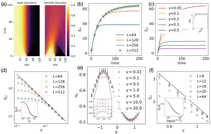
Figure 2: (a) Mean particle density evolutions of generalized monitored free fermions ($L=128$, $\gamma=0.1$) under open boundary conditions (left panel) and periodic boundary conditions (right panel). The feedback induces a strong boundary sensitivity: under OBC the particle density evolves to be evenly distributed, while under OBC the steady state still features the domain structure. (b) Mean dynamics of $S_{\text{cl}}$ for $\gamma=0.05$ for different system sizes. The final saturation values of $S_{\text{cl}}$ depend on the system size $L$ when $L$ is no bigger than the domain wall length $L_{\text{DW}}$. While for sufficiently large size ($L\geq 256$ in this case), $S_{\text{cl}}(t)$ shows no system size dependence. (c) Mean dynamics of $S_{\text{cl}}$ for $L=512$ ($L>L_{\text{DW}}$ for all $\gamma$’s we choose). The data collapse indicates that the saturated evolution $S_{\text{cl}}(t;L>L_{\text{DW}})$ fits into the universal form Eq. (14). (d) Finite size scaling of steady-state $S_{\text{cl}}$, which approach the line $S_{\text{cl}}=c/\gamma$ where $c\approx 3.3$. Inset: data collapse indicates the scaling form $S_{\text{cl}}=L\cdot G(\gamma L)$. (e) Momentum distribution of the steady state, in the periodic boundary conditions. (f) Steady-state $S_{\text{cl}}$ for interacted monitored model, which approach the line $S_{\text{cl}}=\tilde{c}/\gamma^{\nu}$ where $\tilde{c}\approx 1.8$ and $\nu=0.85$. The data collapse indicates the universal scaling form $S_{\text{cl}}=L\cdot\tilde{G}(\gamma L^{1/\nu})$.

3 Feedback-induced skin effect

3.1 Dynamical scale invariance

To quantify the dynamical skin effect induced by feedback, we introduce the classical entropy:

$$S_{\mathrm{cl}}[\{n_{i}\}]\equiv-\sum_{i}\left[n_{i}\log n_{i}+(1-n_{i})\log(1-n_{i})\right].$$ (13)

where only the nontrivial density (i.e., $n_{i}\neq 0,1$) contributes to $S_{\mathrm{cl}}$.

In Fig. 2b, we show the time evolution of the classical entropies $S_{\mathrm{cl}}[\{\overline{\langle n_{i}\rangle}\}]$ starting from $|\psi_{0}\rangle$ under open boundary conditions. We see when the system size is small, $S_{\text{cl}}$ will saturate to a system-size-dependent value. Whereas for large enough systems, the evolution of $S_{\text{cl}}(t)$ will be the same. These numerical simulations support the “domain-wall blurring” picture, where the evolution of $S_{\mathrm{cl}}(t)$ follows a universal pattern when considering a system larger than the size of the domain-wall region (denoted as $L_{\text{DW}}$).

In Fig. 2c, we display $S_{\text{cl}}(t)$ for $L>L_{\text{DW}}$ systems. We observed a scaling form

$$S_{\text{cl}}(\gamma,t,L>L_{\text{DW}})=\frac{1}{\gamma}F(\gamma t),$$ (14)

where the system reaches the steady state with a characteristic relaxation time $t_{\text{rlx}}\sim\gamma^{-1}$, independent of the system size.

Furthermore, we observe that the steady-state $S_{\text{cl}}$ has a scale invariance, as shown in Fig. 2d:

$$S_{\mathrm{cl}}(\gamma,t>t_{\text{rlx}},L)=L\cdot G(\gamma L),$$ (15)

which implies that $L_{\text{DW}}\sim\gamma^{-1}$. In the late-time and thermodynamics limit, the asymptotic behaviors of the scaling functions are

$$F(x\rightarrow\infty)\sim c,\quad G(x\rightarrow\infty)\sim\frac{c}{x},$$ (16)

where $c$ is a numerical constant estimated to be $3.3$ in this specific case. Therefore,

$$S_{\mathrm{cl}}(\gamma,t>t_{\text{rlx}},L>L_{\text{DW}})=\frac{c}{\gamma}\approx\frac{3.3}{\gamma}.$$ (17)

Notably, Equation (15) suggests a scale invariance for the steady-state density profile $n(x)$ in the continuum limit. The finite value of $S_{\text{cl}}$ implies that the feedback-induced skin effect is present even for a vanishingly small measuring rate.

3.2 Suppression of entanglement

One of the consequences of FISE is the suppression of entanglement. Specifically, we prove that $S_{\mathrm{cl}}$ imposes an upper bound for the (trajectory-averaged) steady-state entropy of the monitored dynamics. Consider an arbitrary subsystem $A$ inside the monitored system. The entanglement subadditivity [Nielsen and Chuang(2010), Wilde(2013)] leads to the inequality

$$S_{A}\leq\sum_{i}S_{i}.$$ (18)

Further, consider the reduced density matrix of a local spin at site $i$:

$$\rho_{i}=\begin{bmatrix}n_{i}&o_{i}\\ o_{i}^{*}&1-n_{i}\end{bmatrix},$$ (19)

where $o_{i}$ is the off-diagonal element. Mathematically, the eigenvalues of a positive $2\times 2$ matrix majorize [Horn and Johnson(1991)] the diagonal elements, and thus have less entropy. That is,

$$S_{i} =-\operatorname{Tr}[\rho_{i}\log\rho_{i}]\leq n_{i}\log n_{i}+(1-n_{i})\log(1-n_{i})=S_{\text{cl}}[n_{i}].$$ (20)

Therefore, the entanglement entropy of subregion $A$ is bounded by the classical entropy

$$S_{A}\leq\sum_{i\in A}S_{\text{cl}}[n_{i}]=S_{\text{cl}}[\{n_{i}|i\in A\}].$$ (21)

Also, for a pure state, the entanglement entropy of $A$ is equal to that of its complement $\bar{A}$, i.e., $S_{A}=S_{\bar{A}}$. The classical bound on entanglement entropy also requires

$$S_{A}+S_{\bar{A}}\leq S_{\text{cl}}[\{n_{i}\}],$$ (22)

therefore $S_{A}\leq S_{\mathrm{cl}}/2$.

In the context of entanglement transition in monitored systems, it is natural to consider the trajectory-averaged entanglement, denoted as $\overline{S_{A}}$, which is bounded by $\overline{S_{\text{cl}}[\{\langle n_{i}\rangle\}]}/2$. Since the entropy function is convex, $\overline{S_{A}}$ will also be bounded by:

$$\overline{S_{A}}\leq\frac{1}{2}\overline{S_{\text{cl}}[\{\langle n_{i}\rangle\}]}\leq\frac{1}{2}S_{\text{cl}}\left[\overline{\langle n_{i}\rangle}\right].$$ (23)

The asymptotic behavior, therefore, predicts the area-law entanglement scaling $S\leq c/2\gamma$ for arbitrary $L$, thus proving the area-law entanglement scaling in the $\gamma\rightarrow 0$ limit.

To complete the analysis, in Appendix C.2, we explicitly calculate the trajectory-averaged entanglement entropy (as well as the classical entropy) for the monitored dynamics. We observe that in the periodic boundary conditions, the entanglement entropy scaling indeed undergoes a logarithm-to-area-law transition, while this transition is missing in the open boundary conditions. Also, in order to show the effect of the trajectory variance, as well as find a tighter bound on the entanglement entropy, we calculate the $\overline{S_{\text{cl}}[\{\langle n_{i}\rangle\}]}$.

In the above analysis, we consider only the $\theta=\pi$ case in the feedback operator, while similar FISE appears for arbitrary $\theta$. In Appendix C.3, we show the numerical results for $\theta\neq\pi$. The length of the domain wall, however, is minimized at $\theta=\pi$. When $\theta$ approaches zero, we expect that the FISE still appears, although with a large domain wall that may exceed the numerical simulation capability. Therefore, for the projector $P_{i}$, the FISE is not a fine-tuned phenomenon and may appear for a large class of feedback operations.

3.3 Bulk-edge correspondence

The bulk-edge correspondence of the non-Hermitian effect has been extensively investigated [Zhang et al.(2020)Zhang, Yang, and Fang, Yokomizo and Murakami(2019), Okuma et al.(2020)Okuma, Kawabata, Shiozaki, and Sato, Yang et al.(2020)Yang, Zhang, Fang, and Hu, Borgnia et al.(2020)Borgnia, Kruchkov, and Slager]. In the no-click limit, where the dynamics are described by the non-interacting non-Hermitian Hamiltonian, the skin effect also manifests as a directional bulk current in the periodic boundary systems:

$$J[\{n_{k}\}]\equiv\int_{-\pi}^{+\pi}v_{k}n_{k}dk,$$ (24)

where $n_{k}=\langle c_{k}^{\dagger}c_{k}\rangle$ is the distribution function of the $k$-momentum fermion modes, and $v_{k}=\partial_{k}E(k)$ is the velocity of each quasi-mode.

The rigorous bulk-edge correspondence only happens in the no-click limit, whereas when the quantum jump processes are taken into account, the system lost the single-particle description, and thus the velocity $v_{k}$ becomes ill-defined. However, we can generalize the concept of the directional bulk current $J[\{n_{k}\}]$ at least to the weakly-monitored system, where the velocity $v_{k}$ can be approximated by the result of the free system $v_{k}\approx\partial_{k}E(k)=\sin(k)$.

By simulating the system with identical parameters but under periodic boundary conditions, we show in Fig. 2e that there is an imbalance in the momentum distribution which does not vanish in the $\gamma\rightarrow 0$ limit. Specifically, for $\gamma=0.01$ case, the numerical simulation shows that $J[\{n_{k}\}]\approx-0.94$. This nonzero current serves as another manifestation of the dynamical skin effect at arbitrarily small measurement rates.

3.4 Monitored interacted system

The monitored free-fermion systems belong to a special type of MIPT since the entanglement of the weakly monitored system is not strong, i.e., does not follow the volume-law scaling. From the quantum information point of view, the free fermion systems are not good quantum memory; the initial quantum information will be lost in polynomial time when subject to measurements [Fidkowski et al.(2021)Fidkowski, Haah, and Hastings]. It is therefore necessary to exclude the possibility that FISE only suppresses the logarithm-scaling entanglement.

For the interacting system, it is more convenient to focus on a spin-1/2 Hamiltonian

$$H= \ \sum_{i}\left[J_{1}(\sigma_{i}^{x}\sigma^{x}_{i+1}+\sigma_{i}^{y}\sigma^{y}_{i+1})+J_{z}\sigma_{i}^{z}\sigma^{z}_{i+1}\right.+\left.J_{2}(\sigma_{i}^{x}\sigma^{x}_{i+2}+\sigma_{i}^{y}\sigma^{y}_{i+2})\right].$$ (25)

In Ref. [Fuji and Ashida(2020b)], the non-integrable system (25) under continuous monitoring (on local $\sigma_{i}^{z}$) was shown to display a volume-to-area-law entanglement transition.

In our case, however, we choose the same generalized monitoring as in the free fermion case (via Jordan-Wiger transformation):

$$P_{i}=\frac{1}{2}(\sigma_{i}^{+}-i\sigma_{i+1}^{+})(\sigma_{i}^{-}+i\sigma_{i+1}^{-}),\quad U_{i}=S^{z}_{i+1}.$$ (26)

In the presence of interactions, FISE also manifests in open boundary systems under the influence of this generalized monitoring. The presence of the dynamical skin effect leads to area-law entanglement entropies, allowing for efficient representation of states using matrix-product states [Fannes et al.(1992)Fannes, Nachtergaele, and Werner, D. Perez-Garcia(2007)]. Additionally, the time evolution of large system sizes can be simulated effectively using the TEBD algorithm.

We investigate the steady-state classical entropy for different $\gamma$ values and system sizes up to $L=64$, and fix $J_{1}=0.5$, $J_{z}=1.0$, $J_{2}=0.1$. As shown in Fig. 2f, the numerics indicate that for $\gamma>0.5$, the classical entropy exhibits the asymptotic behavior:

$$S_{\mathrm{cl}}(\gamma,t>t_{\text{rlx}},L>L_{\text{DW}})\approx\frac{\tilde{c}}{\gamma^{\nu}},$$ (27)

where $\tilde{c}=1.8$ and $\nu=0.85$. This suggests that a matrix product state with bond dimension $\chi\sim O(\exp(\gamma^{-\nu}))$ is sufficient to describe the state. However, the numerical simulation becomes challenging in the small $\gamma$ regime. While we are unable to numerically verify the scaling behavior in the small $\gamma$ limit due to computational limitations, our finite-size simulations still demonstrate the scaling law described by (as depicted in Fig. 2f)

$$S_{\text{cl}}(\gamma,t>t_{\text{rlx}})=L\cdot\tilde{G}(\gamma L^{1/\nu}),$$ (28)

where the scaling function shall obey the asymptotic behavior

$$\tilde{G}(x\rightarrow\infty)\sim\frac{\tilde{c}}{x^{\nu}}.$$ (29)

We conjecture that the asymptotic form in Eq. (28) continues to hold in the small-$\gamma$ regime.

(a) Entanglement Entropy scaling	(b) Mutual Information

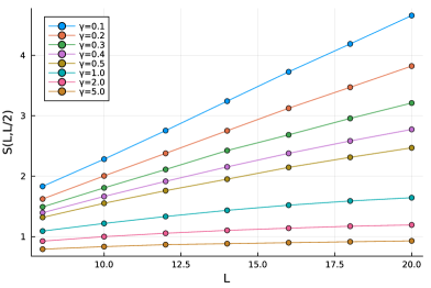
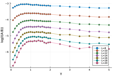
Figure 3: Exact diagonalization simulation of the entanglement dynamics for systems with $J_{1}=J_{z}=0.5$, $J_{2}=0.1$, and under periodic boundary conditions. (a) Trajectory average of entanglement entropy for different measurement rates. (b) Trajectory average of mutual information $I(A:B)$ between two antipodal sites $A$ and $B$. The peak of $I(A:B)$ indicates the critical measurement rate at $\gamma_{c}\approx 1$.

To complete the analysis, we show that under periodic boundary conditions, the usually measurement-induced entanglement appears in this generalized monitored system. We demonstrate this transition using finite-size exact diagonalization. We remark here that the appearance of an entanglement transition can be better revealed from the mutual information $I(A:B)$ shared by two antipodal sites $A$ and $B$. This numerical technique has been used, for example, in Refs. [Li et al.(2019)Li, Chen, and Fisher, Fuji and Ashida(2020a)].

In Fig. 3a, we first demonstrate that for small $\gamma$, the finite size scaling of entanglement entropy $S(L,L/2)$ shows a linear growth in the size $L$. In the large $\gamma$ regime, the entanglement is greatly suppressed, suggesting steady states being area-law entangled. To better demonstrate the existence of an entanglement transition, Fig. 3b displays the mutual information $I(A:B)$. The peak in $I(A:B)$ shows near $\gamma_{c}\approx 1$. Due to the finite size available to the numerical simulation, we are unable to pinpoint the critical measurement rate $\gamma_{c}$.

Therefore, we show that the FISE indeed imposes strong suppression on the entanglement which completely excludes any entanglement transition.

4 Floquet circuits under random measurements

Up till now, we have investigated FISE in the context of the continuously monitored Hamiltonian dynamics. Readers may wonder whether FISE is an artifact of continuous monitoring. This section serves to clarify this question by generalizing the FISE to the quantum circuits under random (generalized) measurements, which is similar to the original setup for the MIPT. The upshot is that only the discrete spatial-temporal translation symmetry is required for the skin effect.

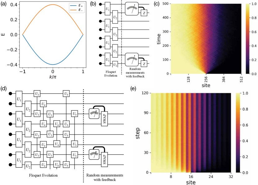
Figure 4: (a) Dispersion relation for circuit model. At the maximal velocity point $k=\pi$, the eigenvectors are $|\pi,-\rangle\approx 0.842|\pi,1\rangle+(0.290-0.455i)|\pi,2\rangle$ and $|\pi,+\rangle\approx(0.290+0.455i)|\pi,1\rangle-0.842|\pi,2\rangle$. (b) Quantum circuit model with Floquet circuit evolution and conditional feedback. (c) Density evolution of the measured Floquet dynamics ($L=512$, $p=0.02$).

4.1 Wave packet motion under Floquet evolution

The notion of discrete quantum circuits naturally appears when we use the Trotter decomposition. In general, when a local Hamiltonian can be decomposed into several groups:

$$H=\sum_{\alpha=1}^{l}H_{\alpha},\quad H_{\alpha}=\sum_{i}o_{\alpha,i},$$ (30)

where each $o_{\alpha,i}$ is a local operator. Within each group, the local operators do not overlap. The time evolution can then be approximated by

$$U(t=N\Delta t)\approx\left(e^{-iH_{1}\Delta t}e^{-iH_{2}\Delta t}\cdots e^{-H_{l}\Delta t}\right)^{N}.$$ (31)

The decomposition approaches the real dynamics in the $\Delta t\rightarrow 0$ limit. While for practical reasons, $\Delta t$ is a finite value, therefore the dynamics described by Eq. (31) is a Floquet dynamics with period $T=l\Delta t$.

We show that the notion of wave packet motion is also valid in the context of the Floquet circuit even when the $\Delta t$ is not vanishing small, as long as the discrete translational symmetry is preserved. For simplicity, we assume that the Floquet circuit has 2-site translational symmetry. We can group two lattice sites into a unit cell and label them as the internal degrees of freedom $a=1,2$. The plane wave is then

$$|k,a\rangle\equiv\frac{1}{\sqrt{L}}\sum_{j}c_{j,a}^{\dagger}e^{-ikj}|0\rangle.$$ (32)

Due to the translational invariance, the evolution $U(T)$ is blocked-diagonal in the momentum space:

$$U_{ab} \equiv\langle k,a|U(T)|k,b\rangle=V(k)\begin{bmatrix}e^{-iE_{+}(k)T}&0\\ 0&e^{-iE_{-}(k)T}\end{bmatrix}V(k)^{\dagger}.$$ (33)

The values $E_{\pm}(k)$ extracted from the eigenvalues of $U_{ab}$ are the quasi-energies of the Floquet dynamics. Consider the branch with quasi-energy $E_{+}$. The wave packet with averaged momentum $k$ and averaged position $x$ has the form

$$|k,x;+\rangle\equiv\int\frac{dp}{2\pi}e^{-\alpha(p-k)^{2}-ix(p-k)}|p,+\rangle,$$ (34)

where $\alpha$ controls the variance of the momentum distribution of the wave packet. After one period $T$, the wave packet evolves to

$$\ U(T)|k,x;+\rangle=\int\frac{dp}{2\pi}e^{-\alpha(p-k)^{2}-ix(p-k)-iE_{+}(p)T}|p,+\rangle$$

$$\propto\int\frac{dp}{2\pi}e^{-\alpha(p-k)^{2}-i\left[x+\frac{E_{+}(p)-E_{+}(k)}{p-k}T\right](p-k)}|p,+\rangle.$$

Specifically, when $\alpha$ is large, most $p$ will be close to $k$, and the movement of the averaged position is approximated by $x\rightarrow x^{\prime}\approx x+E^{\prime}_{+}(k)T$. We therefore restore the wave packet moving picture in the Hamiltonian dynamics, at least for the nearly monochromatic wave packets.

With the picture in mind, we first consider the Floquet dynamics described by the circuits

$$U(T)=\ \prod_{j}\exp\left[-i\left(c_{2j}^{\dagger}c_{2j+1}+c_{2j+1}^{\dagger}c_{2j}\right)T\right]\times\prod_{j}\exp\left[-i\left(c_{2j-1}^{\dagger}c_{2j}+c_{2j}^{\dagger}c_{2j-1}\right)T\right].$$ (35)

We can choose an arbitrary finite value of $T$, say $T=0.5$. The dispersion is then calculated and displayed in Fig. 4a. We remark that for finite $T$, the eigenvectors have shifted compared to the Hamiltonian case. However, the tendency remains the same. That is, the configuration $d^{\dagger}|0\rangle$ still has a bigger overlap with the right-moving wave packet than with the left-moving ones. Therefore, we expect that the feedback-induced skin effect still appears in the Floquet model.

4.2 Skin effect in measured Floquet circuits

Besides the generalization to the Floquet circuit, we show here that the continuous monitoring setup can be replaced with randomly applying strong projective measurement followed by conditional feedback.

Consider the circuit dynamics in Fig. 4b, where the $U_{1}$ and $U_{2}$ come from the Floquet dynamics. Under the Jordan-Wigner transformation, they become

$$U_{1}=U_{2}=\exp\left(-i\frac{T}{2}\sigma_{x}\otimes\sigma_{x}\right)\exp\left(-i\frac{T}{2}\sigma_{y}\otimes\sigma_{y}\right),$$ (36)

and the measurements are the projective measurement of the observable

$$P_{i}=\frac{1}{4}\left(\sigma^{z}_{i}+\sigma^{z}_{i+1}+\sigma^{x}_{i}\sigma^{y}_{i+1}-\sigma_{i}^{y}\sigma^{x}_{i+1}+2\right),$$ (37)

followed by the conditional feedback $U_{i}=\sigma_{i}^{z}$. As displayed in Fig. 4c, for a small measurement rate ($p=0.02$), the feedback still induces the skin effect.

4.3 Experimental proposal on the trapped ions quantum computers

The two-site measurements is hard to realize in the experiments. However, we can device a single-site measured model using a unitary transformation. To formulate the transformation in a clearer way, we temporarily reverse to the fermionic model where the quasi-mode $d_{i}=c_{i}+ic_{i+1}$ are being measured. We now regard $d_{2i-1}$ as the local fermion mode, which corresponds to the transformation

$$d_{2i-1}=\frac{1}{\sqrt{2}}(c_{2i-1}+ic_{2i}),\quad d_{2i}=\frac{1}{\sqrt{2}}(c_{2i}+ic_{2i-1}).$$ (38)

The Hamiltonian is mapped to $H=h_{1}+h_{2}+h_{3}+h_{4}$, where $\{h_{1},h_{2},h_{3},h_{4}\}$ are hopping terms among neighboring unit cells:

$$h_{1} =\sum_{i}\left(d_{2i-1}^{\dagger}d_{2i}+H.c.\right),$$ (39)

$$h_{2} =\frac{1}{2}\sum_{i}\left(d_{2i}^{\dagger}d_{2i+1}+H.c.\right),$$

$$h_{3} =\sum_{i}\left(\frac{i}{2}d_{2i-1}^{\dagger}d_{2i+1}-\frac{i}{2}d_{2i}^{\dagger}d_{2i+2}+H.c.\right),$$

$$h_{4} =\frac{1}{2}\sum_{i}\left(d_{2i-1}^{\dagger}d_{2i+2}+H.c.\right).$$

Under the new basis, the projector becomes an onsite measurement of particle occupation on the odd sites:

$$P_{2i-1}=d_{2i-1}^{\dagger}d_{2i-1},\quad P_{2i}=d_{2i}d^{\dagger}_{2i}.$$ (40)

The feedback operator, however, is not in a neat form on this basis. However, as we remarked, the FISE is not a fine-tuned effect from the feedback, we expect FISE to happen for a wide range of conditional unitary operators. For simplicity, we choose the feedback to be the swap operator on two neighboring sites. To obtain an even simpler model, we keep only half of the measurement $P_{2i-1}$ on the odd sites, and we choose the feedback operator to be the swap gate

$$U_{2i-1}=\operatorname{SWAP}_{2i-1,2i}.$$ (41)

Under the Jordan-Wigner transformation, the measured circuit is displayed in Fig. 4d. The unitary gate $\{U_{1},\cdots,U_{5}\}$ in the circuits are:

$$U_{1} =\mathrm{XX}(\theta)\otimes\mathrm{YY}(\theta),$$ (42)

$$U_{2} =\mathrm{XX}\left(\frac{\theta}{2}\right)\otimes\mathrm{YY}\left(\frac{\theta}{2}\right),$$

$$U_{3} =\mathrm{XY}\left(\frac{\theta}{2}\right)\otimes\mathrm{YX}\left(-\frac{\theta}{2}\right),$$

$$U_{4} =\mathrm{XY}\left(-\frac{\theta}{2}\right)\otimes\mathrm{YX}\left(\frac{\theta}{2}\right),$$

$$U_{5} =\mathrm{XX}\left(\frac{\theta}{2}\right)\otimes\mathrm{YY}\left(\frac{\theta}{2}\right),$$

where $\theta$ is the parameter controlled by the time step of the Trotter decomposition, and the $\mathrm{XX}$, $\mathrm{XY}$, and $\mathrm{YY}$ gates are

$$\mathrm{XX}_{i,j}(\theta) \equiv \exp\left(-i\theta\sigma^{x}_{i}\sigma^{x}_{j}\right),$$ (43)

$$\mathrm{XY}_{i,j}(\theta) \equiv \exp\left(-i\theta\sigma^{x}_{i}\sigma^{y}_{j}\right),$$ (44)

$$\mathrm{YY}_{i,j}(\theta) \equiv \exp\left(-i\theta\sigma^{y}_{i}\sigma^{y}_{j}\right).$$ (45)

The measurement operator is now simply the $\sigma^{z}_{2i-1}$ on odd sites, and the conditional feedback $\operatorname{SWAP}$ (which does not change under Jordan-Wigner transformation) will be applied to the sites ($2i-1$) and ($2i$) when the measurement result in site ($2i-1$) is $-1$.

Experimentally, the trapped ions systems [Paul(1990), Cirac and Zoller(1995), Hayes et al.(2010)Hayes, Matsukevich, Maunz, Hucul, Quraishi, Olmschenk, Campbell, Mizrahi, Senko, and Monroe, Mølmer and Sørensen(1999)] are one of the ideal platforms to realize medium-scale quantum computation and quantum simulations. Using the ${}^{171}\mathrm{Yb}^{+}$ ions trapped by the high-frequency electromagnetic field [Paul(1990)] with fined tune laser pulse, the platform is able to:

1. initiate the state as $|0\cdots 0\rangle$.

2. implement any single-site rotation, which enables to initiate the state to any product state.

3. implement an “Ising” spin-spin interaction [Porras and Cirac(2004), Zhu et al.(2006)Zhu, Monroe, and Duan]: $\mathrm{XX}_{i,j}(\theta)=\exp\left(-i\theta\sigma^{x}_{i}\otimes\sigma^{x}_{j}\right)$.

4. do onsite measurement on $\sigma^{z}$, collapsing qubit to $|0\rangle$ or $|1\rangle$ state.

We remark that, using the combination of single-site and two-site unitary gates, it is possible to realize the YY and XY gates as:

$$\mathrm{XY}_{i,j}(\theta) =\exp\left(-i\frac{\pi}{2}\sigma^{z}_{j}\right)\mathrm{XX}_{i,j}(\theta)\exp\left(i\frac{\pi}{2}\sigma^{z}_{j}\right),$$ (46)

$$\mathrm{YY}_{i,j}(\theta) =\exp\left(-i\frac{\pi}{2}\sigma^{z}_{i}\right)\mathrm{XY}_{i,j}(\theta)\exp\left(i\frac{\pi}{2}\sigma^{z}_{i}\right).$$

Now consider the monitored circuit model displayed in Fig. 4d, where the Floquet dynamics is the Trotterized version of Hamiltonian (39).

The measurement that needs to perform the simple $S^{z}$ measurement, followed by a conditional swap operation, which is

$$U_{\text{SWAP}}\propto\mathrm{XX}\left(\frac{\pi}{4}\right)\otimes\mathrm{YY}\left(\frac{\pi}{4}\right).$$ (47)

In Fig. 4f, we simulate the dynamics on a $32$-qubit chain, and choose $\theta=\pi/4$, with measurement probability $p=0.5$. We see the late time state show a clear feedback-induced skin effect.

5 Conclusion

This work investigates the effect of generalized monitoring on the entanglement phase transition, with a particular focus on the emergence of the skin effect in certain open boundary monitored systems. Our analysis reveals that the skin effect qualitatively alters the entanglement structure of the nonequilibrium steady state, leading to a single area-law phase. Specifically, we show that introducing generic feedback operators can disturb the balance of particle distribution, resulting in particle accumulation. We demonstrate that the FISE is not a fine-tuned phenomenon, as the skin effect appears for different feedback parameters, and survives in the presence of interactions. The suppression of the entanglement entropy from the skin effect also enables an efficient classical simulation of the monitored interacted systems.

These results have practical implications in the context of open systems or controllable quantum devices, as the monitoring-feedback setup can enable the realization of a skin effect without the need for post-selection in non-Hermitian dynamics. For systems showing FISE, the steady states can be reached in constant steps, which is accessible for the noisy intermediate-scale quantum devices. We thus proposed a quantum circuit model displaying FISE which can be experimentally realized on the trapped ions systems.

Note added.— In the middle of this work, we became aware of a recent work [Buchhold et al.(2022)Buchhold, Müller, and Diehl], which also considers the effect of generalized monitoring in the context of MIPT. The two works are complementary to each other: in Ref. [Buchhold et al.(2022)Buchhold, Müller, and Diehl], the authors utilize the feedback (pre-selection) to reveal MIPT as a quantum absorbing state transition that can be directly detected, while our work shows that the presence of conditional feedback may also eliminate the MIPT.

Appendix A Uniqueness of nonequilibrium steady state

In this section, we prove the uniqueness of $\rho_{\mathrm{NESS}}$ for models considered in the main text, by explicitly checking the operator set

$$\mathcal{O}=\{H,L_{1},L_{1}^{\dagger},L_{2},L_{2}^{\dagger},\cdots\}$$ (48)

generates (under multiplication and addition) the complete algebra on the Hilbert space.

A.1 Projective monitoring

We first prove that the Hamiltonian (under open boundary conditions)

$$H=\sum_{i}(c_{i}^{\dagger}c_{i+1}+c_{i+1}^{\dagger}c_{i})$$ (49)

and the projectors

$$P_{i}=\frac{1}{2}(c_{i}^{\dagger}-ic_{i+1}^{\dagger})(c_{i}+ic_{i+1})$$ (50)

generate the whole algebra. Note $H$ and $P_{1}$, $P_{2}$ together generate the following particle number operators:

$$n_{1}-n_{3} =P_{2}-P_{1}+i[H,P_{1}+P_{2}],$$ (51)

$$n_{1}+n_{2} =\frac{1}{2}\left(P_{1}+P_{2}+i[H,n_{1}-n_{3}]+n_{1}-n_{3}\right),$$

$$n_{2}+n_{3} =(n_{1}+n_{2})-(n_{1}-n_{3}).$$

Then, some straightforward algebra lead to

$$c_{1}^{\dagger}c_{2}-c_{2}^{\dagger}c_{1} =i(n_{1}+n_{2})-iP_{1},$$ (52)

$$c_{1}^{\dagger}c_{2}+c_{2}^{\dagger}c_{1} =[c_{1}^{\dagger}c_{2}-c_{2}^{\dagger}c_{1},n_{2}+n_{3}],$$

$$c_{2}^{\dagger}c_{3}-c_{3}^{\dagger}c_{2} =i(n_{2}+n_{3})-iP_{2},$$

$$c_{2}^{\dagger}c_{3}+c_{3}^{\dagger}c_{2} =[n_{1}+n_{2},c_{2}^{\dagger}c_{3}-c_{3}^{\dagger}c_{2}].$$

Upon some addition among Eqs. (52), we obtain the operator $c_{1}^{\dagger}c_{2}$, $c_{2}^{\dagger}c_{3}$ and their Hermitian conjugates. The commutations of them further produce $c_{1}^{\dagger}c_{3}$ and its conjugate. Also, note that

$$[c_{1}^{\dagger}c_{2},c_{2}^{\dagger}c_{1}]=n_{1}-n_{2}.$$ (53)

Together with Eqs. (51), we generate all fermion bilinear terms $c_{i}^{\dagger}c_{j}$ (including $i=j$ case) on sites $(1,2,3)$. To proceed, we subtract the hopping terms between sites $(1,2)$ from $H$. The resulting operator is equivalent to a shorter chain starting from site 2. We can then utilize the calculation above to obtain all $c_{i}^{\dagger}c_{j}$ terms on sites $(2,3,4)$. We eventually obtain all fermion bilinear terms on the chain by applying the strategy iteratively. Note that fermion bilinear terms $c_{i}^{\dagger}c_{j}$ generate the complete algebra within a fixed particle-number sector since any two product states in the sector can be related by applying several fermion hopping terms.

A.2 Generalized monitoring and interactions

For the generalized monitored system described by the jump operators $\{L_{n}=U_{n}P_{n}\}$, the proof of uniqueness is essentially the same as the projective case. Note that we can generate all $P_{i}$ terms by multiplying to jump operators

$$P_{i}=L_{i}^{\dagger}L_{i}.$$ (54)

In this way, we can generate the complete operator algebra in the same way as above.

We argue that the completeness of the operator algebra holds for generic open systems since the exact decoupling of Hilbert space is the result of symmetries or fine-tuning. For the interacting system where the Hamiltonian is

$$H=\sum_{i}(c_{i}^{\dagger}c_{i+1}+c_{i+1}^{\dagger}c_{i}+gn_{i}n_{i+1}).$$ (55)

The above argument means for a random value of $g$, we should expect the completeness of the operator algebra. We can also consider the case where the coupling constant is smoothly varying in the space. In particular, let $g_{i}=0$ for the sites near the boundary. Following the same procedure, we can generate the operator algebra of the subsystem near the boundary. Assume that we meet the first nonzero $g$ at site $i+1$. It means that we have the complete operator algebra (within fixed filling number) $\mathcal{A}_{[1,i]}$ of the subsystem consisting of sites $1,\dots,i$. We first subtract all terms within $\mathcal{A}_{[1,i]}$ from the Hamiltonian and denote the result as $H_{[i+1,N]}$. Consider the commutators

$$=c_{i}^{\dagger}c_{i+1}-c_{i+1}^{\dagger}c_{i},$$ (56)

$$[n_{i-1},c_{i}^{\dagger}c_{i+1}-c_{i+1}^{\dagger}c_{i}] =c_{i}^{\dagger}c_{i+1}+c_{i+1}^{\dagger}c_{i}.$$

In this way, we generate the hopping terms $c_{i}^{\dagger}c_{i+1}$ and $c_{i+1}^{\dagger}c_{i}$. Those terms together with $\mathcal{A}_{[1,i]}$ generate the algebra $\mathcal{A}_{[1,i+1]}$. This procedure can proceed iteratively, therefore producing the complete algebra.

Appendix B Stochastic Schrödinger equation

B.1 Generalized monitoring

Microscopically, a measurement process involves a short-time interaction between the system and the probe, which are initially separable:

$$|\psi_{AB}\rangle=e^{-iH_{\mathrm{int}}\Delta t}|\psi_{A}\rangle\otimes|\psi_{B}\rangle,$$ (57)

where the wave function of the measured system is denoted as $|\psi_{A}\rangle$ and the probe $|\psi_{B}\rangle$. When $\Delta t$ is much smaller than the time scale of the system, the system can be regarded as static during the measurement. Such measurement is called the strong measurement. The probe is thought to be a device that can convert quantum information to the classical one, which takes the form of standard projective measurement. That is, suppose the eigenbasis of the probe is $\{|\phi_{n}\rangle\}$, the probability of getting a record $n$ is

$$p_{n}=\langle\phi_{n}|\rho_{B}|\phi_{n}\rangle,\quad\rho_{B}\equiv\operatorname{Tr}_{A}|\psi_{AB}\rangle\langle\psi_{AB}|,$$ (58)

and the feedback of the measurement to the system is

$$|\tilde{\psi}_{A}^{(n)}\rangle=\langle\phi_{n}|e^{-iH_{\mathrm{int}}\Delta t}|\psi_{A}\rangle\otimes|\psi_{B}\rangle\equiv M_{n}|\psi_{A}\rangle.$$ (59)

The completeness condition requires

$$\sum_{n}\langle\tilde{\psi}_{A}^{(n)}|\tilde{\psi}_{A}^{(n)}\rangle=1\ \Longrightarrow\ \sum_{n}M_{n}^{\dagger}M_{n}=1.$$ (60)

This is the general form of the measure. In the language of density operator, a measurement is described by a set of operators $\{M_{n}\}$. A measurement process may record a result $n$ with probability $p_{n}$ and change the state to:

$$\rho\rightarrow\frac{M_{n}\rho M_{n}^{\dagger}}{\|M_{n}\rho M_{n}^{\dagger}\|}.$$ (61)

If the measurement result is not known, the averaged density matrix after the measurement is

$$\rho\rightarrow\sum_{n}M_{n}\rho M_{n}^{\dagger}.$$ (62)

Such a map is called the quantum channel [Nielsen and Chuang(2010)].

On the other hand, if the strength of system-probe coupling is comparable with the energy scale of the system, which is the case for an open quantum system, the quantum channel expression should depend on time $\Delta t$. This kind of measurement process is called weak measurement. When the system is Markovian (the equation of motion depends only on the near past), the course-grained dissipation process can be described by the channel:

$$M_{n} = L_{n}\sqrt{\gamma\Delta t},$$ (63)

$$M_{0} = \sqrt{1-\sum_{n>0}M_{n}^{\dagger}M_{n}}$$ (64)

$$= 1-\frac{\gamma}{2}\sum_{n>0}L_{n}^{\dagger}L_{n}\Delta t+O(\Delta t^{2}).$$

For the density matrix, the coarse-grained differential equation is the Lindblad equation:

$$\frac{d\rho}{dt} =\lim_{\Delta t\rightarrow 0}\frac{1}{\Delta t}\sum_{n}M_{n}e^{-iH\Delta t}\rho e^{iH\Delta t}M_{n}^{\dagger}$$ (65)

$$=-i[H,\rho]-\frac{\gamma}{2}\sum_{i}\{L_{i}^{\dagger}L_{i},\rho\}+\gamma\sum_{i}L_{i}\rho L_{i}^{\dagger}.$$

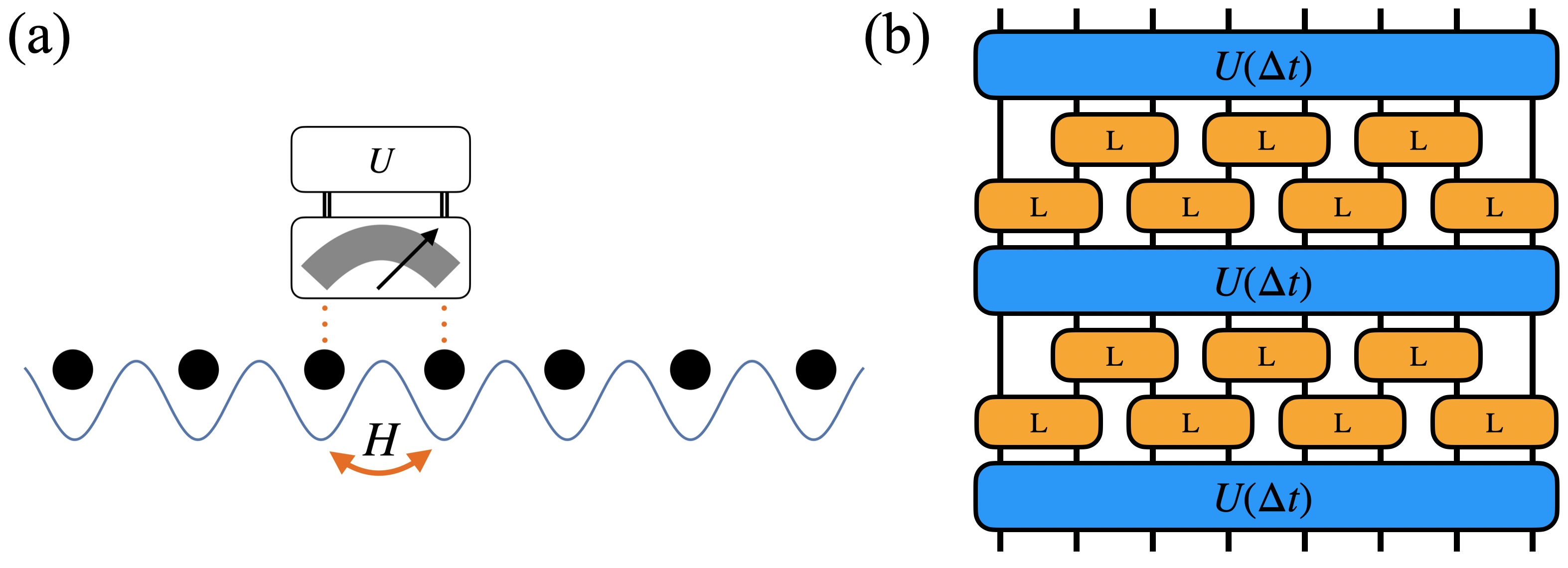
Figure 5: (a) Schematic of a fermion chain under nearest neighbor interaction and generalized monitoring on each pair of neighboring sites. Unitary feedback will be applied if the probe records a quantum jump. (b) Circuits representation of the discretized Hamiltonian evolution with constant monitoring.

The joint dynamics of Hamiltonian evolution and measurement can be equivalently described by the stochastic process, as shown in Fig. 5, where for each time step $\Delta t$, the system first undergoes a coherent evolution $|\psi\rangle\rightarrow e^{-iH\Delta t}|\psi\rangle$, then the application of measurement produces a random process:

$$|\psi\rangle\rightarrow\begin{cases}M_{n}(\Delta t)|\psi\rangle&P_{n}=\langle\psi|L_{n}^{\dagger}L_{n}|\psi\rangle\gamma\Delta t\\ M_{0}(\Delta t)|\psi\rangle&P_{0}=1-\sum_{n>0}P_{n}\end{cases}.$$ (66)

Different records of the measurement result correspond to different trajectories, and the Lindblad equation is equivalent to the trajectory averaged of such stochastic processes. In the continuum limit, the stochastic differential equation can be formulated by introducing a Poisson random variable $dW_{n}$ taking the discrete values of $0$ or $1$. The $dW_{n}=1$ case corresponds to registering a quantum jump, otherwise, $dW_{n}=0$. The expectation value for random $dW_{n}$ is proportional to $dt$:

$$\overline{dW}_{n}=\langle\psi|L_{n}^{\dagger}L_{n}|\psi\rangle\gamma dt.$$ (67)

Different $dW_{n}$’s are independent, i.e., they satisfy the orthogonal condition

$$dW_{m}dW_{n}=\delta_{mn}dW_{m}.$$ (68)

Therefore, the random quantum jump process $|\psi\rangle\rightarrow M_{n}|\psi\rangle$ is described by the expression

$$d|\psi\rangle=\left(\frac{L_{n}}{\sqrt{\langle L_{n}^{\dagger}L_{n}\rangle}}-1\right)|\psi\rangle dW_{n},$$ (69)

and the null-detection case correspond to $|\psi\rangle\rightarrow M_{0}|\psi\rangle$, which is described by a non-Hermitian differential equation:

$$d|\psi\rangle=-\frac{\gamma}{2}\sum_{m}(L_{m}^{\dagger}L_{m}-\langle L_{m}^{\dagger}L_{m}\rangle)|\psi\rangle dt,$$ (70)

where the $\langle L_{m}^{\dagger}L_{m}\rangle$ is introduced for the normalization purpose. Together with the coherent evolution, we obtain the stochastic Schrödinger equation in the main text:

$$d|\psi\rangle= \ \left[-iH-\frac{\gamma}{2}\sum_{m}(L_{m}^{\dagger}L_{m}-\langle L_{m}^{\dagger}L_{m}\rangle)\right]|\psi\rangle dt+\sum_{m}\left(\frac{L_{m}}{\sqrt{\langle L_{m}^{\dagger}L_{m}\rangle}}-1\right)|\psi\rangle dW_{m}.$$ (71)

B.2 Free fermion simulation

For numerical simulation of Eq. (71), we can first discretize the time into small interval $\Delta t$. The discrete evolution is then

$$|\psi(t+\Delta t)\rangle=\mathcal{M}_{\Delta t}[e^{-iH_{\mathrm{eff}}\Delta t}|\psi(t)\rangle],$$ (72)

where $\mathcal{M}_{\Delta t}$ represents the quantum jump that randomly happened in time interval $\Delta t$:

$$\mathcal{M}_{\Delta t}[|\psi\rangle]\propto\prod_{m\in I}L_{m}|\psi\rangle.$$ (73)

In the Eq. (73), the set $I$ denotes the random jump processes, which can be obtained by

$$I=\{n|r_{n}<\gamma\langle L_{n}^{\dagger}L_{n}\rangle\Delta t\},$$ (74)

where $\{r_{n}\in(0,1)\}$ is a set of independent random variables with evenly distributed probability.

The free fermion system can be efficiently represented by the Gaussian state [Bravyi(2004)]. For a particle number conserving system, the Gaussian state is a quasimode-occupied state, represented by a matrix $B$:

$$|B\rangle\equiv\prod_{j=1}^{N}\sum_{i}B_{ij}c_{i}^{\dagger}|0\rangle=\bigotimes_{j=1}^{N}|B_{j}\rangle,$$ (75)

where each column $B_{j}$ is an occupied quasimode. Note that there is an SU($N$) gauge freedom for the matrix $B$, i.e.,

$$|B^{\prime}\rangle=|BU\rangle=|B\rangle,$$ (76)

where $U$ is an arbitrary SU($N$) matrix. Such gauge freedom implies that a Gaussian state is entirely specified by the linear subspace spanned by the quasimodes $B_{i}$’s.

The random Schrödinger equation can be Trotterized as Eq. (72). Using the Baker-Campbell-Hausdor formula $e^{A}Be^{-A}=e^{\operatorname{ad}_{A}}B$, the nonunitary evolution is

$$e^{-iH_{\mathrm{eff}}\Delta t}|B_{t}\rangle =\prod_{j=1}^{N}\sum_{i}B_{ij}e^{-iH_{\mathrm{eff}}\Delta t}c_{i}^{\dagger}e^{iH_{\mathrm{eff}}\Delta t}|0\rangle$$

$$=\prod_{j=1}^{N}\sum_{i}B_{ij}e^{-i\Delta t[H_{\mathrm{eff}},\cdot]}c_{i}^{\dagger}|0\rangle$$

$$=\prod_{j=1}^{N}\sum_{i}\sum_{k}B_{ij}c_{k}^{\dagger}\left[e^{-iH_{\mathrm{eff}}\Delta t}\right]_{ki}|0\rangle$$

$$=\prod_{j=1}^{N}\sum_{k}\left[e^{-iH_{\mathrm{eff}}\Delta t}B_{ij}\right]_{kj}c_{k}^{\dagger}|0\rangle$$

$$=|e^{-iH_{\mathrm{eff}}\Delta t}B_{t}\rangle.$$

That is, the matrix is multiplied by the exponential of the effective non-Hermitian (single-body) Hamiltonian matrix. Note that the resulting matrix is not orthogonal anymore, while the state is still well-defined by the linear space spanned by those unorthogonal vectors. In general, for a Gaussian state represented by matrix $B$, we can obtain a canonical form for the representing matrix using the QR decomposition $B=Q\cdot R$, where $Q$ is a unitary matrix and $R$ is upper triangular. Note that $Q$ and $B$ span the same linear space, so the Gaussian state can be expressed as $|Q\rangle$.

The supper operator $\mathcal{M}_{\Delta t}$ in Eq. (72) corresponds to the Poisson jump process, where for each index $i$, we randomly decide whether a quantum jump process

$$|B\rangle\rightarrow\frac{L_{i}|B\rangle}{\|L_{i}|B\rangle\|}$$ (77)

happens, with the probability

$$p_{i}=\langle B|L_{i}^{\dagger}L_{i}|B\rangle\gamma\Delta t$$ (78)

The $L_{m}$’s we choose in the main text have the form

$$L_{m}=e^{ih}d^{\dagger}d,\quad d^{\dagger}=\sum_{i}a_{i}c_{i}^{\dagger},\quad h=\sum_{ij}h_{ij}c_{i}^{\dagger}c_{j},$$ (79)

where $d^{\dagger}$ is a quasimode, and $h$ is a fermion bilinear. The following shows that the Gaussian form is preserved by such jump operator $L_{m}$. First, the probability of the jump process is

$$\langle B|L_{m}^{\dagger}L_{m}|B\rangle=\langle B|d^{\dagger}d|B\rangle=\|d|B\rangle\|^{2}.$$

The action of annihilation operator $d$ on $|B\rangle$ is

$$d|B\rangle=\sum_{k}a_{k}^{*}c_{k}\prod_{j}\sum_{i}c_{i}^{\dagger}B_{ij}|0\rangle=\sum_{j}\langle a|B_{j}\rangle\bigotimes_{l\neq j}|B_{l}\rangle,$$ (80)

so we can obtain the probability

$$p_{m}=\sum_{j}|\langle a|B_{j}\rangle|^{2}\gamma\Delta t.$$ (81)

Besides, we can utilize the gauge freedom to choose the basis such that $\langle a|B^{\prime}_{j}\rangle=0$ for $j>1$. The matrix $B^{\prime}$ always exists since we can always find a column $j$ that $\langle a|B_{j}\rangle\neq 0$ (otherwise, the probability of the jump is zero). We then move the column to the first and define the column as

$$|B^{\prime}_{j}\rangle=|B_{j}\rangle-\frac{\langle a|B_{j}\rangle}{\langle a|B_{1}\rangle}|B_{1}\rangle,\quad j>1.$$ (82)

Note that such column transformation does not alter the linear space $B$ spans, while the orthogonality and the normalization might be affected and should be renormalized afterward. Eq. (80) then simplified to:

$$d|B\rangle=\bigotimes_{j>1}|B^{\prime}_{j}\rangle.$$ (83)

The result of the quantum jump is

$$L_{m}|B\rangle=|e^{ih}a\rangle\bigotimes_{j>1}|e^{ih}B^{\prime}_{j}\rangle.$$ (84)

The representation of the outcome state is also not orthogonal. An additional QR decomposition is needed to convert it to canonical form.

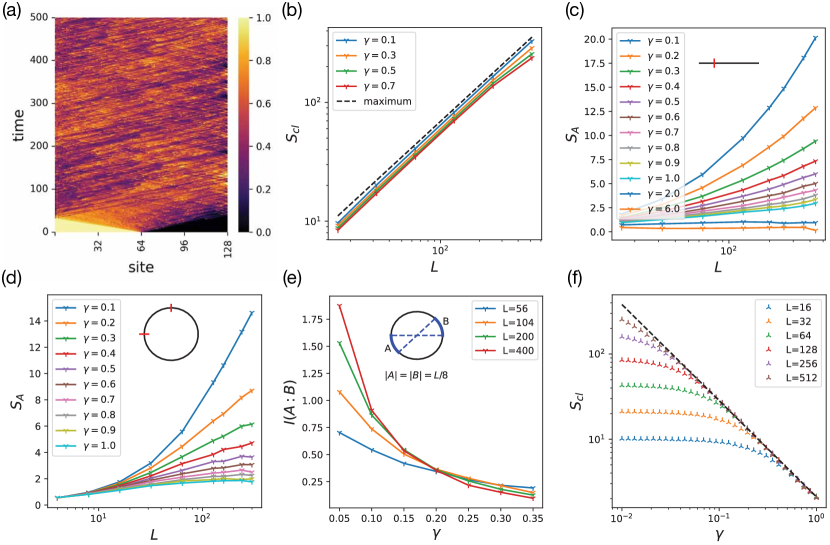
Figure 6: (a) Density evolution under projective monitoring with $\gamma=0.1$ for a single trajectory. (b) Scaling of steady-state classical entropies. (c) Scaling of entanglement entropies. (d) Trajectory average of entanglement entropy for different measurement rates. (e) Trajectory average of mutual information $I(A:B)$ between two $L/8$ antipodal segments $A$ and $B$. The crossing of $I(A:B)$ indicates the critical measurement rate at $\gamma_{c}\approx 0.2$. (f) Trajectory average of classical entropy for systems in different sizes.

Appendix C Numerical simulations of the monitored free fermion dynamics

C.1 Projective monitoring

We have demonstrated that a general Lindblad equation,

$$\frac{d}{dt}\rho=-i\left[H,\rho\right]+\gamma\sum_{i}L_{i}\rho L_{i}^{\dagger}-\frac{1}{2}\left\{L_{i}^{\dagger}L_{i},\rho\right\},$$ (85)

where $L_{i}$ are projectors, leads to a unique and homogeneous steady state (under open boundary conditions). In this section, we present numerical evidence supporting the homogeneity of late-time states for typical stochastic trajectories, described by:

$$d|\psi\rangle= \ \left[-iH-\frac{\gamma}{2}\sum_{m}(L_{m}^{\dagger}L_{m}-\langle L_{m}^{\dagger}L_{m}\rangle)\right]|\psi\rangle dt+\sum_{m}\left(\frac{L_{m}}{\sqrt{\langle L_{m}^{\dagger}L_{m}\rangle}}-1\right)|\psi\rangle dW_{m}.$$ (86)

That is, the spatial homogeneity is not only at the density matrix level but also at the trajectory level. This suggests that the skin effect, which suppresses entanglement entropy, does not arise within the projective monitoring system. Therefore, introducing conditional feedback is essential to induce a dynamical skin effect.

In the following, we consider the model studied in the main text, of which the unitary evolution is generated by the Hamiltonian:

$$H=\sum_{i}(c^{\dagger}_{i}c_{i+1}+c^{\dagger}_{i+1}c_{i})$$ (87)

and the monitoring is described by

$$L_{i}=\frac{1}{2}(c^{\dagger}_{i}-ic^{\dagger}_{i+1})(c_{i}+ic_{i+1}).$$ (88)

First, Fig. 6a displays the particle density evolution of a typical trajectory. At late times, the system reaches a homogeneous state with only minor fluctuations. To further analyze the homogeneity of trajectories’ densities, in Fig. 6b, we plot the trajectory-averaged classical entropy:

$$S_{\text{cl}}=-\overline{\sum_{i}\left[\langle n_{i}\rangle\log\langle n_{i}\rangle+(1-\langle n_{i}\rangle)\log(1-\langle n_{i}\rangle\right]}.$$ (89)

We observe a linear growth with system size, indicating a highly homogeneous density distribution. Moreover, when $\gamma$ is small, the growth of the classical entropy approaches the saturation value

$$S_{\text{max}}=L\log 2,$$ (90)

which means that most trajectory has nearly homogeneous density distribution.

In contrast, Fig. 6c shows the entanglement entropy, which is considerably smaller than the classical entropy and exhibits an entanglement transition from log law to area law. These results suggest that the projective monitoring system under open boundary conditions may undergo a measurement-induced entanglement phase transition, similar to the periodic boundary condition.

C.2 Generalized monitoring

Fig. 6d illustrates the trajectory averaging of entanglement entropy. The entanglement entropy exhibits a transition from log law to area law. We can pinpoint the critical measurement rate $\gamma_{c}$ by doing the scaling analysis of the mutual information between two antipodal regions (as displayed in Fig. 6e).

In the main text, we have demonstrated trajectory averaging of classical entropy $\overline{S_{\text{cl}}[\{\langle n_{i}\rangle\}]}$ provides an upper bound on entanglement entropy $S_{A}$ and is itself bounded by classical entropy of averaged particle number:

$$\overline{S_{\text{cl}}[\{\langle n_{i}\rangle\}]}\leq S_{\text{cl}}[\{\overline{\langle n_{i}\rangle}\}]$$ (91)

In this section, we instead calculate $\overline{S_{\text{cl}}[\{\langle n_{i}\rangle\}]}$ which imposes a tighter bound on the entanglement entropy. As displayed in Fig. 6f, $\overline{S_{\text{cl}}[\{\langle n_{i}\rangle\}]}$ behaves similarly as $S_{\text{cl}}[\{\overline{\langle n_{i}\rangle}\}]$ but with slightly different slop, indicating an asymptotic form:

$$\overline{S_{\text{cl}}[\{\langle n_{i}\rangle\}]}\simeq\frac{2.1}{\gamma^{\nu}}$$ (92)

where the scaling factor $\nu\approx 1.13$ instead of $1$ for $S_{\text{cl}}[\{\overline{\langle n_{i}\rangle}\}]$.

C.3 Generalized monitoring with different conditional feedback

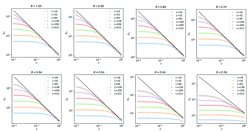
Figure 7: Steady-state classical entropies $\overline{S_{\text{cl}}[\langle n_{i}\rangle]}$ for feedback $U_{i}=\exp(i\theta n_{i+1})$, where we chose $\theta$ from $\pi$ to $0.3\pi$. the data points all approach the asymptotic line $\nu\log\gamma+\log S_{\mathrm{cl}}=c^{\prime}(\theta)$ where $\nu\approx 1.13$ in the thermodynamic limit.

In this appendix, we provide more numerical results on the monitored free fermion system with Hamiltonian

$$H=\sum_{i}(c_{i}^{\dagger}c_{i+1}+c_{i+1}^{\dagger}c_{i})$$ (93)

and the generalized monitoring characterized by the projective monitoring

$$P_{i}=\frac{1}{2}(c_{i}^{\dagger}-ic_{i+1}^{\dagger})(c_{i}+ic_{i+1})$$ (94)

followed by the conditional feedback $U_{i}=e^{i\theta n_{i+1}}$ on site ($i+1$).

In this section, we demonstrate numerically, that even under different parameters $\theta$’s apart from the $\theta=\pi$, the feedback-induced skin effect also appears. Therefore it is not a fin-tuned property of generalized monitoring. We will characterize the skin effect using the trajectory-averaged classical entropy:

$$S^{\theta}_{\text{cl}}(\gamma,L)\equiv\overline{S_{\text{cl}}[\{\langle n_{i}\rangle\}]}.$$ (95)

In Fig. 7, we show that The steady-state classical entropies in the thermodynamic limit $L\rightarrow\infty$ all satisfy the general asymptotic behaviors:

$$S^{\theta}_{\mathrm{cl}}(\gamma,L\rightarrow\infty)=\frac{c_{\theta}}{\gamma^{\nu}},$$ (96)

where $\nu\approx 1.13$, while the constant $c_{\theta}$ increases as $\theta$ decreases:

$$\theta/\pi$$

As discussed in the main text, the constant $c_{\theta}$ determines the spatial extents of the domain wall. The finite data point we obtained implies that $c_{\theta}$ increases exponentially fast when $\theta\rightarrow 0$. In the $\theta=0$ case, $c_{\theta}$ diverges and there is no skin effect.

The large-size domain walls impose significant overhead for numerical simulations. For small $\theta$ ($\leq 0.3\pi$), accessing the thermodynamic limit becomes practically hard.

Based on the numerical results, we speculate the scaling form (96) holds for different $\theta$ and $\gamma$. Therefore we expect the skin effect to arise in a large class of generalized monitored systems.

References

- [Alberton et al.(2021)Alberton, Buchhold, and Diehl] O. Alberton, M. Buchhold, and S. Diehl. Entanglement transition in a monitored free-fermion chain: From extended criticality to area law. Phys. Rev. Lett., 126:170602, Apr 2021. doi: 10.1103/PhysRevLett.126.170602. URL https://link.aps.org/doi/10.1103/PhysRevLett.126.170602.
- [Bao et al.(2020)Bao, Choi, and Altman] Yimu Bao, Soonwon Choi, and Ehud Altman. Theory of the phase transition in random unitary circuits with measurements. Phys. Rev. B, 101:104301, Mar 2020. doi: 10.1103/PhysRevB.101.104301. URL https://link.aps.org/doi/10.1103/PhysRevB.101.104301.
- [Barchielli and Gregoratti(2009)] Alberto Barchielli and Matteo Gregoratti. The Stochastic Schrödinger Equation, pages 11–49. Springer Berlin Heidelberg, Berlin, Heidelberg, 2009. ISBN 978-3-642-01298-3. doi: 10.1007/978-3-642-01298-3˙2. URL https://doi.org/10.1007/978-3-642-01298-3_2.
- [Berdanier et al.(2019)Berdanier, Marino, and Altman] William Berdanier, Jamir Marino, and Ehud Altman. Universal dynamics of stochastically driven quantum impurities. Phys. Rev. Lett., 123:230604, Dec 2019. doi: 10.1103/PhysRevLett.123.230604. URL https://link.aps.org/doi/10.1103/PhysRevLett.123.230604.
- [Biella and Schiró(2021)] Alberto Biella and Marco Schiró. Many-Body Quantum Zeno Effect and Measurement-Induced Subradiance Transition. Quantum, 5:528, August 2021. ISSN 2521-327X. doi: 10.22331/q-2021-08-19-528. URL https://doi.org/10.22331/q-2021-08-19-528.
- [Borgnia et al.(2020)Borgnia, Kruchkov, and Slager] Dan S. Borgnia, Alex Jura Kruchkov, and Robert-Jan Slager. Non-hermitian boundary modes and topology. Phys. Rev. Lett., 124:056802, Feb 2020. doi: 10.1103/PhysRevLett.124.056802. URL https://link.aps.org/doi/10.1103/PhysRevLett.124.056802.
- [Bravyi(2004)] Sergey Bravyi. Lagrangian representation for fermionic linear optics. 2004. doi: 10.48550/ARXIV.QUANT-PH/0404180. URL https://arxiv.org/abs/quant-ph/0404180.
- [Breuer and Petruccione(2007)] Heinz-Peter Breuer and Francesco Petruccione. The Theory of Open Quantum Systems. Oxford University Press, 01 2007. ISBN 9780199213900. doi: 10.1093/acprof:oso/9780199213900.001.0001. URL https://doi.org/10.1093/acprof:oso/9780199213900.001.0001.
- [Buchhold et al.(2021)Buchhold, Minoguchi, Altland, and Diehl] M. Buchhold, Y. Minoguchi, A. Altland, and S. Diehl. Effective theory for the measurement-induced phase transition of dirac fermions. Phys. Rev. X, 11:041004, Oct 2021. doi: 10.1103/PhysRevX.11.041004. URL https://link.aps.org/doi/10.1103/PhysRevX.11.041004.
- [Buchhold et al.(2022)Buchhold, Müller, and Diehl] M. Buchhold, T. Müller, and S. Diehl. Revealing measurement-induced phase transitions by pre-selection, 2022.
- [Cao et al.(2019)Cao, Tilloy, and Luca] Xiangyu Cao, Antoine Tilloy, and Andrea De Luca. Entanglement in a fermion chain under continuous monitoring. SciPost Phys., 7:024, 2019. doi: 10.21468/SciPostPhys.7.2.024. URL https://scipost.org/10.21468/SciPostPhys.7.2.024.
- [Carollo and Alba(2022)] Federico Carollo and Vincenzo Alba. Entangled multiplets and spreading of quantum correlations in a continuously monitored tight-binding chain. Phys. Rev. B, 106:L220304, Dec 2022. doi: 10.1103/PhysRevB.106.L220304. URL https://link.aps.org/doi/10.1103/PhysRevB.106.L220304.
- [Chan et al.(2018)Chan, De Luca, and Chalker] Amos Chan, Andrea De Luca, and J. T. Chalker. Solution of a minimal model for many-body quantum chaos. Phys. Rev. X, 8:041019, Nov 2018. doi: 10.1103/PhysRevX.8.041019. URL https://link.aps.org/doi/10.1103/PhysRevX.8.041019.
- [Chan et al.(2019)Chan, Nandkishore, Pretko, and Smith] Amos Chan, Rahul M. Nandkishore, Michael Pretko, and Graeme Smith. Unitary-projective entanglement dynamics. Phys. Rev. B, 99:224307, Jun 2019. doi: 10.1103/PhysRevB.99.224307. URL https://link.aps.org/doi/10.1103/PhysRevB.99.224307.
- [Chen et al.(2020)Chen, Li, Fisher, and Lucas] Xiao Chen, Yaodong Li, Matthew P. A. Fisher, and Andrew Lucas. Emergent conformal symmetry in nonunitary random dynamics of free fermions. Phys. Rev. Research, 2:033017, Jul 2020. doi: 10.1103/PhysRevResearch.2.033017. URL https://link.aps.org/doi/10.1103/PhysRevResearch.2.033017.
- [Choi et al.(2020)Choi, Bao, Qi, and Altman] Soonwon Choi, Yimu Bao, Xiao-Liang Qi, and Ehud Altman. Quantum error correction in scrambling dynamics and measurement-induced phase transition. Phys. Rev. Lett., 125:030505, Jul 2020. doi: 10.1103/PhysRevLett.125.030505. URL https://link.aps.org/doi/10.1103/PhysRevLett.125.030505.
- [Cirac and Zoller(1995)] J. I. Cirac and P. Zoller. Quantum computations with cold trapped ions. Phys. Rev. Lett., 74:4091–4094, May 1995. doi: 10.1103/PhysRevLett.74.4091. URL https://link.aps.org/doi/10.1103/PhysRevLett.74.4091.
- [Coppola et al.(2022)Coppola, Tirrito, Karevski, and Collura] Michele Coppola, Emanuele Tirrito, Dragi Karevski, and Mario Collura. Growth of entanglement entropy under local projective measurements. Phys. Rev. B, 105:094303, Mar 2022. doi: 10.1103/PhysRevB.105.094303. URL https://link.aps.org/doi/10.1103/PhysRevB.105.094303.
- [D. Perez-Garcia(2007)] M.M. Wolf J.I. Cirac D. Perez-Garcia, F. Verstraete. Matrix product state representations, 2007.
- [Daley(2014)] Andrew J. Daley. Quantum trajectories and open many-body quantum systems. Advances in Physics, 63(2):77–149, 2014. doi: 10.1080/00018732.2014.933502. URL https://doi.org/10.1080/00018732.2014.933502.
- [Davies(1974)] E. B. Davies. Markovian master equations. Communications in Mathematical Physics, 39(2):91–110, 1974. doi: 10.1007/BF01608389. URL https://doi.org/10.1007/BF01608389.
- [Evans(1977)] David E. Evans. Irreducible quantum dynamical semigroups. Communications in Mathematical Physics, 54(3):293–297, 1977. doi: 10.1007/BF01614091. URL https://doi.org/10.1007/BF01614091.
- [Fannes et al.(1992)Fannes, Nachtergaele, and Werner] M. Fannes, B. Nachtergaele, and R. F. Werner. Finitely correlated states on quantum spin chains. Communications in Mathematical Physics, 144(3):443–490, 1992. doi: 10.1007/BF02099178. URL https://doi.org/10.1007/BF02099178.
- [Fidkowski et al.(2021)Fidkowski, Haah, and Hastings] Lukasz Fidkowski, Jeongwan Haah, and Matthew B. Hastings. How Dynamical Quantum Memories Forget. Quantum, 5:382, January 2021. ISSN 2521-327X. doi: 10.22331/q-2021-01-17-382. URL https://doi.org/10.22331/q-2021-01-17-382.
- [Fisher et al.(2022a)Fisher, Khemani, Nahum, and Vijay] Matthew P. A. Fisher, Vedika Khemani, Adam Nahum, and Sagar Vijay. Random quantum circuits, 2022a.
- [Fisher et al.(2022b)Fisher, Khemani, Nahum, and Vijay] Matthew P. A. Fisher, Vedika Khemani, Adam Nahum, and Sagar Vijay. Random quantum circuits, 2022b.
- [Fishman et al.(2020)Fishman, White, and Stoudenmire] Matthew Fishman, Steven R. White, and E. Miles Stoudenmire. The ITensor software library for tensor network calculations, 2020.
- [Frigerio(1978)] Alberto Frigerio. Stationary states of quantum dynamical semigroups. Communications in Mathematical Physics, 63(3):269–276, 1978. doi: 10.1007/BF01196936. URL https://doi.org/10.1007/BF01196936.
- [Fuji and Ashida(2020a)] Yohei Fuji and Yuto Ashida. Measurement-induced quantum criticality under continuous monitoring. Phys. Rev. B, 102:054302, Aug 2020a. doi: 10.1103/PhysRevB.102.054302. URL https://link.aps.org/doi/10.1103/PhysRevB.102.054302.
- [Fuji and Ashida(2020b)] Yohei Fuji and Yuto Ashida. Measurement-induced quantum criticality under continuous monitoring. Phys. Rev. B, 102:054302, Aug 2020b. doi: 10.1103/PhysRevB.102.054302. URL https://link.aps.org/doi/10.1103/PhysRevB.102.054302.
- [Gopalakrishnan and Gullans(2021)] Sarang Gopalakrishnan and Michael J. Gullans. Entanglement and purification transitions in non-hermitian quantum mechanics. Phys. Rev. Lett., 126:170503, Apr 2021. doi: 10.1103/PhysRevLett.126.170503. URL https://link.aps.org/doi/10.1103/PhysRevLett.126.170503.
- [Gullans and Huse(2020a)] Michael J. Gullans and David A. Huse. Scalable probes of measurement-induced criticality. Phys. Rev. Lett., 125:070606, Aug 2020a. doi: 10.1103/PhysRevLett.125.070606. URL https://link.aps.org/doi/10.1103/PhysRevLett.125.070606.
- [Gullans and Huse(2020b)] Michael J. Gullans and David A. Huse. Dynamical purification phase transition induced by quantum measurements. Phys. Rev. X, 10:041020, Oct 2020b. doi: 10.1103/PhysRevX.10.041020. URL https://link.aps.org/doi/10.1103/PhysRevX.10.041020.
- [Gullans et al.(2021)Gullans, Krastanov, Huse, Jiang, and Flammia] Michael J. Gullans, Stefan Krastanov, David A. Huse, Liang Jiang, and Steven T. Flammia. Quantum coding with low-depth random circuits. Phys. Rev. X, 11:031066, Sep 2021. doi: 10.1103/PhysRevX.11.031066. URL https://link.aps.org/doi/10.1103/PhysRevX.11.031066.
- [Hatano and Nelson(1996)] Naomichi Hatano and David R. Nelson. Localization transitions in non-hermitian quantum mechanics. Phys. Rev. Lett., 77:570–573, Jul 1996. doi: 10.1103/PhysRevLett.77.570. URL https://link.aps.org/doi/10.1103/PhysRevLett.77.570.
- [Hayes et al.(2010)Hayes, Matsukevich, Maunz, Hucul, Quraishi, Olmschenk, Campbell, Mizrahi, Senko, and Monroe] D. Hayes, D. N. Matsukevich, P. Maunz, D. Hucul, Q. Quraishi, S. Olmschenk, W. Campbell, J. Mizrahi, C. Senko, and C. Monroe. Entanglement of atomic qubits using an optical frequency comb. Phys. Rev. Lett., 104:140501, Apr 2010. doi: 10.1103/PhysRevLett.104.140501. URL https://link.aps.org/doi/10.1103/PhysRevLett.104.140501.
- [Horn and Johnson(1991)] Roger A. Horn and Charles R. Johnson. Topics in Matrix Analysis. Cambridge University Press, 1991. doi: 10.1017/CBO9780511840371.
- [Iadecola et al.(2022)Iadecola, Ganeshan, Pixley, and Wilson] Thomas Iadecola, Sriram Ganeshan, J. H. Pixley, and Justin H. Wilson. Dynamical entanglement transition in the probabilistic control of chaos, 2022.
- [Ippoliti and Khemani(2021)] Matteo Ippoliti and Vedika Khemani. Postselection-free entanglement dynamics via spacetime duality. Phys. Rev. Lett., 126:060501, Feb 2021. doi: 10.1103/PhysRevLett.126.060501. URL https://link.aps.org/doi/10.1103/PhysRevLett.126.060501.
- [Ippoliti et al.(2021a)Ippoliti, Gullans, Gopalakrishnan, Huse, and Khemani] Matteo Ippoliti, Michael J. Gullans, Sarang Gopalakrishnan, David A. Huse, and Vedika Khemani. Entanglement phase transitions in measurement-only dynamics. Phys. Rev. X, 11:011030, Feb 2021a. doi: 10.1103/PhysRevX.11.011030. URL https://link.aps.org/doi/10.1103/PhysRevX.11.011030.
- [Ippoliti et al.(2021b)Ippoliti, Gullans, Gopalakrishnan, Huse, and Khemani] Matteo Ippoliti, Michael J. Gullans, Sarang Gopalakrishnan, David A. Huse, and Vedika Khemani. Entanglement phase transitions in measurement-only dynamics. Phys. Rev. X, 11:011030, Feb 2021b. doi: 10.1103/PhysRevX.11.011030. URL https://link.aps.org/doi/10.1103/PhysRevX.11.011030.
- [Ippoliti et al.(2022)Ippoliti, Rakovszky, and Khemani] Matteo Ippoliti, Tibor Rakovszky, and Vedika Khemani. Fractal, logarithmic, and volume-law entangled nonthermal steady states via spacetime duality. Phys. Rev. X, 12:011045, Mar 2022. doi: 10.1103/PhysRevX.12.011045. URL https://link.aps.org/doi/10.1103/PhysRevX.12.011045.
- [Jacobs and Steck(2006)] Kurt Jacobs and Daniel A. Steck. A straightforward introduction to continuous quantum measurement. Contemporary Physics, 47(5):279–303, 2006. doi: 10.1080/00107510601101934. URL https://doi.org/10.1080/00107510601101934.
- [Jian et al.(2020)Jian, You, Vasseur, and Ludwig] Chao-Ming Jian, Yi-Zhuang You, Romain Vasseur, and Andreas W. W. Ludwig. Measurement-induced criticality in random quantum circuits. Phys. Rev. B, 101:104302, Mar 2020. doi: 10.1103/PhysRevB.101.104302. URL https://link.aps.org/doi/10.1103/PhysRevB.101.104302.
- [Jian et al.(2022)Jian, Bauer, Keselman, and Ludwig] Chao-Ming Jian, Bela Bauer, Anna Keselman, and Andreas W. W. Ludwig. Criticality and entanglement in non-unitary quantum circuits and tensor networks of non-interacting fermions, 2022.
- [Jian et al.(2021)Jian, Yang, Bi, and Chen] Shao-Kai Jian, Zhi-Cheng Yang, Zhen Bi, and Xiao Chen. Yang-lee edge singularity triggered entanglement transition. Phys. Rev. B, 104:L161107, Oct 2021. doi: 10.1103/PhysRevB.104.L161107. URL https://link.aps.org/doi/10.1103/PhysRevB.104.L161107.
- [Kawabata et al.(2022)Kawabata, Numasawa, and Ryu] Kohei Kawabata, Tokiro Numasawa, and Shinsei Ryu. Entanglement phase transition induced by the non-hermitian skin effect, 2022.
- [Kells et al.(2023)Kells, Meidan, and Romito] Graham Kells, Dganit Meidan, and Alessandro Romito. Topological transitions in weakly monitored free fermions. SciPost Phys., 14:031, 2023. doi: 10.21468/SciPostPhys.14.3.031. URL https://scipost.org/10.21468/SciPostPhys.14.3.031.
- [Ladewig et al.(2022)Ladewig, Diehl, and Buchhold] B. Ladewig, S. Diehl, and M. Buchhold. Monitored open fermion dynamics: Exploring the interplay of measurement, decoherence, and free hamiltonian evolution. Phys. Rev. Research, 4:033001, Jul 2022. doi: 10.1103/PhysRevResearch.4.033001. URL https://link.aps.org/doi/10.1103/PhysRevResearch.4.033001.
- [Lavasani et al.(2021)Lavasani, Alavirad, and Barkeshli] Ali Lavasani, Yahya Alavirad, and Maissam Barkeshli. Measurement-induced topological entanglement transitions in symmetric random quantum circuits. Nature Physics, 17(3):342–347, 2021. doi: 10.1038/s41567-020-01112-z. URL https://doi.org/10.1038/s41567-020-01112-z.
- [Li and Fisher(2021)] Yaodong Li and Matthew P. A. Fisher. Statistical mechanics of quantum error correcting codes. Phys. Rev. B, 103:104306, Mar 2021. doi: 10.1103/PhysRevB.103.104306. URL https://link.aps.org/doi/10.1103/PhysRevB.103.104306.
- [Li et al.(2018)Li, Chen, and Fisher] Yaodong Li, Xiao Chen, and Matthew P. A. Fisher. Quantum zeno effect and the many-body entanglement transition. Phys. Rev. B, 98:205136, Nov 2018. doi: 10.1103/PhysRevB.98.205136. URL https://link.aps.org/doi/10.1103/PhysRevB.98.205136.
- [Li et al.(2019)Li, Chen, and Fisher] Yaodong Li, Xiao Chen, and Matthew P. A. Fisher. Measurement-driven entanglement transition in hybrid quantum circuits. Phys. Rev. B, 100:134306, Oct 2019. doi: 10.1103/PhysRevB.100.134306. URL https://link.aps.org/doi/10.1103/PhysRevB.100.134306.
- [Li et al.(2021a)Li, Chen, Ludwig, and Fisher] Yaodong Li, Xiao Chen, Andreas W. W. Ludwig, and Matthew P. A. Fisher. Conformal invariance and quantum nonlocality in critical hybrid circuits. Phys. Rev. B, 104:104305, Sep 2021a. doi: 10.1103/PhysRevB.104.104305. URL https://link.aps.org/doi/10.1103/PhysRevB.104.104305.
- [Li et al.(2021b)Li, Vasseur, Fisher, and Ludwig] Yaodong Li, Romain Vasseur, Matthew P. A. Fisher, and Andreas W. W. Ludwig. Statistical mechanics model for clifford random tensor networks and monitored quantum circuits, 2021b. URL https://arxiv.org/abs/2110.02988.
- [Lindblad(1976)] G. Lindblad. On the generators of quantum dynamical semigroups. Communications in Mathematical Physics, 48(2):119–130, 1976. doi: 10.1007/BF01608499. URL https://doi.org/10.1007/BF01608499.
- [Lopez-Piqueres et al.(2020)Lopez-Piqueres, Ware, and Vasseur] Javier Lopez-Piqueres, Brayden Ware, and Romain Vasseur. Mean-field entanglement transitions in random tree tensor networks. Phys. Rev. B, 102:064202, Aug 2020. doi: 10.1103/PhysRevB.102.064202. URL https://link.aps.org/doi/10.1103/PhysRevB.102.064202.
- [Martinez Alvarez et al.(2018)Martinez Alvarez, Barrios Vargas, and Foa Torres] V. M. Martinez Alvarez, J. E. Barrios Vargas, and L. E. F. Foa Torres. Non-hermitian robust edge states in one dimension: Anomalous localization and eigenspace condensation at exceptional points. Phys. Rev. B, 97:121401(R), Mar 2018. doi: 10.1103/PhysRevB.97.121401. URL https://link.aps.org/doi/10.1103/PhysRevB.97.121401.
- [Minato et al.(2022)Minato, Sugimoto, Kuwahara, and Saito] Takaaki Minato, Koudai Sugimoto, Tomotaka Kuwahara, and Keiji Saito. Fate of measurement-induced phase transition in long-range interactions. Phys. Rev. Lett., 128:010603, Jan 2022. doi: 10.1103/PhysRevLett.128.010603. URL https://link.aps.org/doi/10.1103/PhysRevLett.128.010603.
- [Mølmer and Sørensen(1999)] Klaus Mølmer and Anders Sørensen. Multiparticle entanglement of hot trapped ions. Phys. Rev. Lett., 82:1835–1838, Mar 1999. doi: 10.1103/PhysRevLett.82.1835. URL https://link.aps.org/doi/10.1103/PhysRevLett.82.1835.
- [Müller et al.(2022)Müller, Diehl, and Buchhold] T. Müller, S. Diehl, and M. Buchhold. Measurement-induced dark state phase transitions in long-ranged fermion systems. Phys. Rev. Lett., 128:010605, Jan 2022. doi: 10.1103/PhysRevLett.128.010605. URL https://link.aps.org/doi/10.1103/PhysRevLett.128.010605.
- [Nahum et al.(2018)Nahum, Vijay, and Haah] Adam Nahum, Sagar Vijay, and Jeongwan Haah. Operator spreading in random unitary circuits. Phys. Rev. X, 8:021014, Apr 2018. doi: 10.1103/PhysRevX.8.021014. URL https://link.aps.org/doi/10.1103/PhysRevX.8.021014.
- [Nahum et al.(2021)Nahum, Roy, Skinner, and Ruhman] Adam Nahum, Sthitadhi Roy, Brian Skinner, and Jonathan Ruhman. Measurement and entanglement phase transitions in all-to-all quantum circuits, on quantum trees, and in landau-ginsburg theory. PRX Quantum, 2:010352, Mar 2021. doi: 10.1103/PRXQuantum.2.010352. URL https://link.aps.org/doi/10.1103/PRXQuantum.2.010352.
- [Nielsen and Chuang(2010)] Michael A. Nielsen and Isaac L. Chuang. Quantum Computation and Quantum Information: 10th Anniversary Edition. Cambridge University Press, 2010. doi: 10.1017/CBO9780511976667.
- [Okuma et al.(2020)Okuma, Kawabata, Shiozaki, and Sato] Nobuyuki Okuma, Kohei Kawabata, Ken Shiozaki, and Masatoshi Sato. Topological origin of non-hermitian skin effects. Phys. Rev. Lett., 124:086801, Feb 2020. doi: 10.1103/PhysRevLett.124.086801. URL https://link.aps.org/doi/10.1103/PhysRevLett.124.086801.
- [Paul(1990)] Wolfgang Paul. Electromagnetic traps for charged and neutral particles. Rev. Mod. Phys., 62:531–540, Jul 1990. doi: 10.1103/RevModPhys.62.531. URL https://link.aps.org/doi/10.1103/RevModPhys.62.531.
- [Porras and Cirac(2004)] D. Porras and J. I. Cirac. Effective quantum spin systems with trapped ions. Phys. Rev. Lett., 92:207901, May 2004. doi: 10.1103/PhysRevLett.92.207901. URL https://link.aps.org/doi/10.1103/PhysRevLett.92.207901.
- [Prosen(2015)] Tomaž Prosen. Matrix product solutions of boundary driven quantum chains. Journal of Physics A: Mathematical and Theoretical, 48(37):373001, aug 2015. doi: 10.1088/1751-8113/48/37/373001. URL https://doi.org/10.1088/1751-8113/48/37/373001.
- [Skinner et al.(2019)Skinner, Ruhman, and Nahum] Brian Skinner, Jonathan Ruhman, and Adam Nahum. Measurement-induced phase transitions in the dynamics of entanglement. Phys. Rev. X, 9:031009, Jul 2019. doi: 10.1103/PhysRevX.9.031009. URL https://link.aps.org/doi/10.1103/PhysRevX.9.031009.
- [Spohn(1980)] Herbert Spohn. Kinetic equations from hamiltonian dynamics: Markovian limits. Rev. Mod. Phys., 52:569–615, Jul 1980. doi: 10.1103/RevModPhys.52.569. URL https://link.aps.org/doi/10.1103/RevModPhys.52.569.
- [Torres(2019)] Luis E F Foa Torres. Perspective on topological states of non-hermitian lattices. Journal of Physics: Materials, 3(1):014002, nov 2019. doi: 10.1088/2515-7639/ab4092. URL https://doi.org/10.1088/2515-7639/ab4092.
- [Turkeshi and Schiró(2023)] Xhek Turkeshi and Marco Schiró. Entanglement and correlation spreading in non-hermitian spin chains. Phys. Rev. B, 107:L020403, Jan 2023. doi: 10.1103/PhysRevB.107.L020403. URL https://link.aps.org/doi/10.1103/PhysRevB.107.L020403.
- [Turkeshi et al.(2021)Turkeshi, Biella, Fazio, Dalmonte, and Schiró] Xhek Turkeshi, Alberto Biella, Rosario Fazio, Marcello Dalmonte, and Marco Schiró. Measurement-induced entanglement transitions in the quantum ising chain: From infinite to zero clicks. Phys. Rev. B, 103:224210, Jun 2021. doi: 10.1103/PhysRevB.103.224210. URL https://link.aps.org/doi/10.1103/PhysRevB.103.224210.
- [Turkeshi et al.(2022a)Turkeshi, Dalmonte, Fazio, and Schirò] Xhek Turkeshi, Marcello Dalmonte, Rosario Fazio, and Marco Schirò. Entanglement transitions from stochastic resetting of non-hermitian quasiparticles. Phys. Rev. B, 105:L241114, Jun 2022a. doi: 10.1103/PhysRevB.105.L241114. URL https://link.aps.org/doi/10.1103/PhysRevB.105.L241114.
- [Turkeshi et al.(2022b)Turkeshi, Piroli, and Schiró] Xhek Turkeshi, Lorenzo Piroli, and Marco Schiró. Enhanced entanglement negativity in boundary-driven monitored fermionic chains. Phys. Rev. B, 106:024304, Jul 2022b. doi: 10.1103/PhysRevB.106.024304. URL https://link.aps.org/doi/10.1103/PhysRevB.106.024304.
- [Vasseur et al.(2019)Vasseur, Potter, You, and Ludwig] Romain Vasseur, Andrew C. Potter, Yi-Zhuang You, and Andreas W. W. Ludwig. Entanglement transitions from holographic random tensor networks. Phys. Rev. B, 100:134203, Oct 2019. doi: 10.1103/PhysRevB.100.134203. URL https://link.aps.org/doi/10.1103/PhysRevB.100.134203.
- [von Keyserlingk et al.(2018)von Keyserlingk, Rakovszky, Pollmann, and Sondhi] C. W. von Keyserlingk, Tibor Rakovszky, Frank Pollmann, and S. L. Sondhi. Operator hydrodynamics, otocs, and entanglement growth in systems without conservation laws. Phys. Rev. X, 8:021013, Apr 2018. doi: 10.1103/PhysRevX.8.021013. URL https://link.aps.org/doi/10.1103/PhysRevX.8.021013.
- [Wilde(2013)] Mark M. Wilde. Quantum Information Theory. Cambridge University Press, 2013. doi: 10.1017/CBO9781139525343.
- [Wiseman and Milburn(2009)] Howard M. Wiseman and Gerard J. Milburn. Quantum Measurement and Control. Cambridge University Press, 2009. doi: 10.1017/CBO9780511813948.
- [Yang et al.(2020)Yang, Zhang, Fang, and Hu] Zhesen Yang, Kai Zhang, Chen Fang, and Jiangping Hu. Non-hermitian bulk-boundary correspondence and auxiliary generalized brillouin zone theory. Phys. Rev. Lett., 125:226402, Nov 2020. doi: 10.1103/PhysRevLett.125.226402. URL https://link.aps.org/doi/10.1103/PhysRevLett.125.226402.
- [Yang et al.(2022)Yang, Li, Fisher, and Chen] Zhi-Cheng Yang, Yaodong Li, Matthew P. A. Fisher, and Xiao Chen. Entanglement phase transitions in random stabilizer tensor networks. Phys. Rev. B, 105:104306, Mar 2022. doi: 10.1103/PhysRevB.105.104306. URL https://link.aps.org/doi/10.1103/PhysRevB.105.104306.
- [Yao and Wang(2018)] Shunyu Yao and Zhong Wang. Edge states and topological invariants of non-hermitian systems. Phys. Rev. Lett., 121:086803, Aug 2018. doi: 10.1103/PhysRevLett.121.086803. URL https://link.aps.org/doi/10.1103/PhysRevLett.121.086803.
- [Yokomizo and Murakami(2019)] Kazuki Yokomizo and Shuichi Murakami. Non-bloch band theory of non-hermitian systems. Phys. Rev. Lett., 123:066404, Aug 2019. doi: 10.1103/PhysRevLett.123.066404. URL https://link.aps.org/doi/10.1103/PhysRevLett.123.066404.
- [Zabalo et al.(2020)Zabalo, Gullans, Wilson, Gopalakrishnan, Huse, and Pixley] Aidan Zabalo, Michael J. Gullans, Justin H. Wilson, Sarang Gopalakrishnan, David A. Huse, and J. H. Pixley. Critical properties of the measurement-induced transition in random quantum circuits. Phys. Rev. B, 101:060301(R), Feb 2020. doi: 10.1103/PhysRevB.101.060301. URL https://link.aps.org/doi/10.1103/PhysRevB.101.060301.
- [Zhang et al.(2020)Zhang, Yang, and Fang] Kai Zhang, Zhesen Yang, and Chen Fang. Correspondence between winding numbers and skin modes in non-hermitian systems. Phys. Rev. Lett., 125:126402, Sep 2020. doi: 10.1103/PhysRevLett.125.126402. URL https://link.aps.org/doi/10.1103/PhysRevLett.125.126402.
- [Zhou and Nahum(2019)] Tianci Zhou and Adam Nahum. Emergent statistical mechanics of entanglement in random unitary circuits. Phys. Rev. B, 99:174205, May 2019. doi: 10.1103/PhysRevB.99.174205. URL https://link.aps.org/doi/10.1103/PhysRevB.99.174205.
- [Zhu et al.(2006)Zhu, Monroe, and Duan] Shi-Liang Zhu, C. Monroe, and L.-M. Duan. Arbitrary-speed quantum gates within large ion crystals through minimum control of laser beams. Europhysics Letters, 73(4):485, jan 2006. doi: 10.1209/epl/i2005-10424-4. URL https://dx.doi.org/10.1209/epl/i2005-10424-4.