FRECKLL: Full and Reduced Exoplanet Chemical Kinetics distiLLed

Abstract

We introduce a new chemical kinetic code FRECKLL (Full and Reduced Exoplanet Chemical Kinetics distiLLed) to evolve large chemical networks efficiently. FRECKLL employs ‘distillation’ in computing the reaction rates, which minimizes the error bounds to the minimum allowed by double precision values ($\epsilon\leq 10^{-15}$). FRECKLL requires less than 5 minutes to evolve the full Venot2020 network in a 130 layers atmosphere and 30 seconds to evolve the Venot2020 reduced scheme. Packaged with FRECKLL is a TauREx 3.1 plugin for usage in forward modelling and retrievals. We present TauREx retrievals performed on a simulated HD189733 JWST spectra using the full and reduced Venot2020 chemical networks and demonstrate the viability of total disequilibrium chemistry retrievals and the ability for JWST to detect disequilibrium processes.

1 Introduction

In the last decade, observations from space using mainly the Hubble Space Telescope (HST) and the Spitzer Space Telescope (Spitzer) and from the ground, have allowed to characterise the atmospheric properties of a handful of planets from their transit (Tinetti et al., 2007; Kreidberg et al., 2014; Sing et al., 2016; Sedaghati et al., 2017; Wakeford et al., 2017; Tsiaras et al., 2018; Fisher & Heng, 2018; Anisman et al., 2020; Edwards et al., 2021; Gressier et al., 2022; Wong et al., 2022; Saba et al., 2022; Changeat et al., 2022), eclipse (Swain et al., 2008; Crouzet et al., 2014; Haynes et al., 2015; Line et al., 2016; Edwards et al., 2020; Line et al., 2014; Changeat & Edwards, 2021; Fu et al., 2022) or phase-curve observations (Stevenson et al., 2017; Arcangeli et al., 2019; Changeat et al., 2021; Changeat, 2022; Mikal-Evans et al., 2022; Chubb & Min, 2022). Due to the low resolution and narrow wavelength coverage of older generation space-based instrumentation, however, degeneracies can often lead to multiple interpretations of exoplanet spectra, depending on model and prior assumptions (e.g. Changeat et al., 2020b). To explore the information contained in these spectra, exoplanet teams have developed sophisticated methods to invert the information content in the spectra of exoplanets. These methods, often called spectral retrieval techniques (Irwin et al., 2008; Madhusudhan & Seager, 2009; Benneke & Seager, 2012; Line et al., 2013; Waldmann et al., 2015; Min et al., 2020; Mollière et al., 2019; Al-Refaie et al., 2021b) require the evaluation of thousands to millions of forward models, therefore requiring significant computing resources. Often, the computing requirements imply that simplified atmospheric models have to be employed, for instance, by assuming 1-dimensional geometries and other idealized assumptions on the thermal structure, the chemistry and the cloud properties. Since the information extracted from current spectra is low, assumptions are commonly used throughout the literature. These assumptions include isothermal thermal structure, constant chemical profiles or equilibrium chemistry, and fully opaque cloud opacities.

In retrieval schemes, the chemistry is often recovered using profiles that are constant with altitude; a single free parameter then represents each molecule. While not representative of an entire atmosphere, current observations mostly probe small pressure regions where chemical variations remain small. An alternative assumption is thermochemical equilibrium (White et al., 1958; Eriksson et al., 1971), which requires computing the chemistry state by minimizing the Gibbs free energy of the system. Such an assumption has gained popularity due to the reduced degrees of freedom. Furthermore, it often only requires two free parameters for metallicity and the C/O ratio chosen for their natural links to planetary formation and evolution processes. Equilibrium chemistry, however, is a strong assumption with little justification, given that our knowledge of exoplanetary atmospheres is still in its infancy. Furthermore, simulations employing kinetics methods and thus taking into account disequilibrium processes such as mixing and photochemistry have proven that chemical equilibrium is inadequate in many scenarios (e.g. Moses et al. 2011, 2013, 2016; Venot et al. 2012, 2014, 2020a, 2020b; Molaverdikhani et al. 2019; Tsai et al. 2021). With future telescopes, accurate representation of the chemical processes will be essential to ensure unbiased interpretation of the observations as discussed in the first analyses of JWST data (The JWST Transiting Exoplanet Community Early Release Science Team et al., 2022).

In this paper we present the first implementation of a full chemical kinetic scheme into an atmospheric retrieval framework. We use the flexibility of the plugin system in TauREx 3.1 to integrate this new scheme and explore the use of chemical kinetic models in atmospheric retrievals. In particular, we focus our study on quantifying the impact of the equilibrium chemistry assumption in interpreting atmospheres exhibiting disequilibrium processes. Section 2 presents our implementation of the chemical kinetic code and the steps carried out in this work. In Section 3, we present the results of our simulations. Finally, Section 4 discusses our findings and provides the main conclusions of our exploration.

2 Kinetic Model

2.1 Description of chemical kinetic model

As opposed to thermochemical equilibrium models, which predict the chemical state of a planet’s atmosphere by minimising the Gibbs free energy of the system, chemical kinetic models necessitate integrating the system of differential equations representing each considered reactions until a steady-state is reached. The continuity equation (Equation 1) describes the temporal evolution of the abundance of each species $i$, considering a one-dimensional plane-parallel atmosphere.

$$\frac{\partial n_{i}}{\partial t}=P_{i}-L_{i}-\frac{\partial\phi_{i}}{\partial z}$$ (1)

where $n_{i}$, $P_{i}$ and $L_{i}$ are the number density (cm^-3), production rate and loss rate of species $i$ (cm^-3.s^-1), $z$ is the vertical coordinate of the atmosphere, and $\phi_{i}$ is the vertical flux for species $i$ which has the form of a diffusion equation given in Equation 2.

$$\phi_{i}=-n_{i}D_{i}\left(\frac{1}{n_{i}}\frac{\partial n_{i}}{\partial z}+\frac{1}{H_{i}}+\frac{1}{T}\frac{\partial T}{\partial z}\right)-n_{i}K_{zz}\frac{\partial n_{i}}{\partial z}$$ (2)

Here, $D_{i}$ is the molecular diffusion coefficient (cm².s^-1), $H_{i}$ is the scale height for species $i$ (km), T is the temperature (K) and $K_{zz}$ is the eddy diffusion coefficient (cm².s^-1).

At $t=0$ s, an initial abundance is set. FRECKLL can accept any initial atmospheric abundance, either user-supplied or from an external code. As the default, the system is initialised with the abundance of each species assumed to be at thermochemical equilibrium. This initial state is computed using the ACE code (Agúndez et al., 2012) and, subsequently, Equation 1 is evolved using a stiff ODE solver such as VODE (Brown et al., 1989) or DLSODES from the ODEPACK (Hindmarsh, 1983) package until steady state is achieved or a user-defined condition is reached. Metallicity, C/O and N/O ratios can be set to determine the initial abundance produced by ACE. In addition to those parameters, the model also allows for the definition of the eddy diffusion parameter $K_{zz}$, this given as a constant value or layer-by-layer. For a 100 layer atmosphere, FRECKLL takes roughly 4–5 minutes to reach a steady-state, using the full chemical network of Venot et al. (2020a) involving 108 species, 1906 reactions and 55 photodissociations. The model also included the reduced network of Venot et al. (2020a), which includes 44 species and 582 reactions, speeding-up the convergence of the model to roughly 30 seconds.

2.2 The importance of Numerical stability

Improving numerical stability is of utmost importance in ensuring a solution can converge and, moreover, converge quickly. One of the challenges with chemical kinetics is the inherent stiffness of the equations. This stiffness arises from the chemical timescales and abundances, which involve an extensive range of magnitudes. Integration requires stiff ODE algorithms such as Backwards differentiation formula, Rosenbrock and backwards Euler methods which can vary the time steps over large orders of magnitude. Additionally, an overlooked aspect involves the computation of sums. With double precision we generally expect the upper bound of relative errors from rounding to be $\epsilon_{m}\approx 10^{-6}$. Assuming a function implemented with algorithm $f(x)$ and the true function $\tilde{f}(x)$ the relative error for an algorithm $\epsilon$ is computed as:

$$\epsilon=\frac{|f(x)-\tilde{f}(x)|}{|\tilde{f}(x)|}$$ (3)

Here, the true function is $\tilde{f}(x)=\sum^{n}x_{i}$ where summation is performed at infinite precision. We must also consider the condition number $C$:

$$C=\frac{\sum^{n}{|x_{i}|}}{|\sum^{n}{x_{i}}|}$$ (4)

which represents the intrinsic sensitivity of summation. For naive summation such as the inbuilt python sum function, the error is bounded as:

$$\epsilon\leq n\epsilon_{m}C$$ (5)

where $n$ is the number of elements. The error for pairwise summation used by the numpy.sum function is bounded by:

$$\epsilon\leq\frac{\epsilon_{m}log_{2}n}{1-\epsilon_{m}log_{2}n}C$$ (6)

Generally, well-conditioned problems are those where $C\approx 1$, one such case is where all values are non-negative (i.e $x_{i}>0$). For 10,000 elements, the error from naive summation is $\epsilon\leq 10^{-12}$ and for pairwise we expect an error $\epsilon\leq 10^{-15}$.

The problem comes when dealing with extensive magnitudes and a mixture of negative and non-negative values. To illustrate, lets us take an array of values $x=[10^{16},10^{30},1,5,10,10^{4},-10^{30},-10^{16}]$, where $\sum x=10016$. Attempting to use the native sum we get:

⬇

>>> sum( [1e+16, 1e+30, 1, 5, 10,

10000.0, -1e+30, -1e+16])

-7638326771712.0

the error is in the order of $\epsilon\approx 10^{8}$. Pairwise summation performs a little better:

⬇

>>> numpy.sum( [1e+16, 1e+30, 1, 5,

10, 10000.0, -1e+30, -1e+16])

0.0

here $\epsilon=1$. The problem is ill-conditioned with a condition number of $C=10^{26}$ which is extremely large. This arises from catastrophic cancellation where precision limits for floating points mean $dbl(10^{30}+1)=10^{30}$ where $dbl$ is an operation under double-precision. For kinetics calculations, this is problematic, as summing production and loss rates for a molecule can suddenly become zero, change sign or magnitude. In the Jacobian, these appear as sudden discontinuities and can cause stiff ODE methods to oscillate at certain times and continually reduce the time-step, which will drop the integration efficiency. To avoid these problems in FRECKLL, we instead employ the K-fold summation method (Ogita et al., 2005). This method first performs an error-free transformation of an array:

⬇

def twosum(a,b):

x = a + b

z = x - a

y = (a - (x-z)) + (b-z)

return x,y

\pardef vecsum(x):

for i in range(1, len(x)):

a,b = twosum(x[i], x[i-1])

x[i] = a

x[i-1] = b

return x

The twosum computes the resultant floating point sum and residuals from the summation. For each element $i$, the result is stored at $i$ and the residual at $i-1$. For an array $x$ the algorithm produces a resultant array $y$ where $y=vecsum(x)$ which has the property:

$$\sum^{n}y_{i}=\sum^{n}x_{i}$$ (7)

assuming infinite precision. This is often referred to as ‘distillation’ (Kahan, 1987). For low condition numbers, elements $i=1...n-1$ will be zero and $i=n$ will contain the resultant sum (i.e $y_{n}=\sum^{n}x_{i}$). For higher condition numbers this takes the form $\sum_{n-1}y_{i}+y_{n}=\sum x_{i}$. Distillation has the effect of reducing the condition number and indeed, applying it to our original array $x=[10^{16},10^{30},1,5,10,10^{4},-10^{30},-10^{16}]$, the condition number falls to $C\approx 10^{9}$. As distillation preserves the original sum and reduces the condition number, we can apply it $K-1$ times until we reach our desired condition number before applying the summation; this is K-fold summation in its essence:

⬇

def kfold(x, K):

v = x

for k in range(K-1):

v = vecsum(v)

\parreturn sum(v[:-1]) + v[-1]

\par>>> kfold( [1e+16, 1e+30, 1, 5, 10,

10000.0, -1e+30, -1e+16], K=2)

10016.0

Applying this algorithm for $K=2$ we indeed get the correct result. The error bounds for $K=2$ are $\epsilon_{K=2}\leq 10^{4}$. Increasing to $K=4$ gives an error bounded $\epsilon_{K=4}\leq 10^{-15}$ which is the maximum possible with double precision. K-fold summation is significantly slower than numpy.sum; 10,000 elements takes roughly 7-10x longer than numpy. However, as we will demonstrate, the increase in precision greatly benefits convergence. We employ K-fold summation in computing the production and loss rates of molecules. To maximise computational efficiency and precision we combine the rates into a single array. For molecule $i$ and reaction $r$ we combine the production rate $P^{i}_{r}$ and loss rate $L^{i}_{r}$ into a total molecule rate $R^{i}$. If we have $p$ production reactions and $l$ loss reactions then:

$$\begin{split}R^{i}_{1...p}&=P^{i}_{1...p}\\ R^{i}_{p+1...p+l}&=-L^{i}_{1...l}\\ \end{split}$$ (8)

The total rate for molecule $i$ is given as:

$$R_{i}=k(R^{i}_{r},K=4)$$ (9)

where $k$ is our K-fold function. We can rewrite Equation 2 as:

$$\frac{\partial n_{i}}{\partial t}=R_{i}-\frac{\partial\phi_{i}}{\partial z}$$ (10)

We demonstrate the benefit of k-fold summation by solving a benchmark system. We compute a HD 209458 b model between $10^{-5}$–$10^{2}$ bar, using the thermal and vertical mixing profiles from Venot et al. (2020a) displayed in Figure 1. The model consists of 130 layers, 108 molecules, 1906 reactions and 55 photodissociations from the Venot2020 network (Venot et al., 2020a). We evolve the system with a relative tolerance of $10^{-3}$ and absolute tolerance at $10^{-25}$ until $t=10^{10}$ s with steady-state occurring at $t=10^{8}$ s.

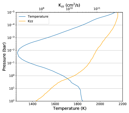
Figure 1: Temperature and vertical mixing ($K_{zz}$) profiles of HD 209458 b taken from Venot et al. (2020a).

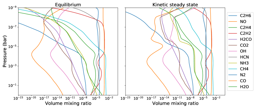
Figure 2: Chemical abundances for a benchmark HD 209458 b atmosphere using temperature and mixing profiles from Venot et al. (2020a). The left plot is the initial state of the system at equilibrium abundances and right is the final steady state solution at $t=10^{10}$s.

Figure 2 shows the initial abundances at equlibrium computed using ACE and the final steady state solution achieved by FRECKLL at $t=10^{10}$ s. Using piecewise summation implemented by numpy.sum takes roughly 128 minutes to evolve until $t=10^{10}$ s requiring 467335 function evaluations and 2179 jacobian evaluations. The issue is that the solver is unable to take larger time steps, especially at $t\approx 10^{8}$ s where $\Delta t\approx 10^{4}$ s. As discontinuities appear more often, the solver is forced to use small timesteps in order to ensure smoothness in the function. This effect becomes more pronounced as the system approaches steady state as the solver has difficultly integrating certain $|\frac{\partial n_{i}}{\partial t}|$ below $10^{-10}$.

Solving the same system using K-fold summation until $t=10^{10}$ s takes 5 minutes, 2,682 function evaluations and 158 jacobian evaluations. As we stated previously, K-fold summation is significantly slower than piecewise summation but we manage to gain a 25x reduction in solver time as well as a 175x reduction in function evaluations. The improved precision means that $|\frac{\partial n_{i}}{\partial t}|$ can reach $10^{-15}$ and the solver is choosing larger time-steps that skip from $10^{8}$s$-10^{10}$ s. In fact, solving further to $10^{12}$ s takes only 10 extra function evaluations.

There is always a trade-off between raw performance and precision. When dealing with stiff non-linear systems, convergence can be hampered by the underlying precision of algorithms. It is sometimes easy to forget that summation is also an algorithm and not an intrinsic feature of computation. We demonstrate that choosing a slower, more precise summation algorithm can lead to significant performance gains from faster convergence.

3 Forward Models

FRECKLL includes a plugin for TauREx 3.1 (Al-Refaie et al., 2021b, a) for generation of synthetic spectra and retrievals using the chemical kinetic code. We demonstrate its forward modelling capabilities by simulating HD 189733 b with parameters taken from the literature which are given in Table 1. Note that we simulate HD 189733 b with a constant $K_{zz}$ of 4$\times$10⁸ cm².s^-1, meaning that we can expect vertical mixing to be important in this scenario. For simplicity, the temperature profile for those simulations is modelled using an isothermal profile, even if radiative transfer models predict variations with altitude, as well as with longitude and latitude (e.g. Drummond et al., 2020). In the model, we include absorption using the ExoMol line-lists (Tennyson & Yurchenko, 2012; Chubb et al., 2021; Tennyson et al., 2020) from the species H₂O (Polyansky et al., 2018), CH₄ (Yurchenko & Tennyson, 2014), CO (Li et al., 2015), CO₂ (Yurchenko et al., 2020), NH₃ (Coles et al., 2019), HCN (Harris et al., 2006), C₂H₂ (Chubb et al., 2020), C₂H₄ (Mant et al., 2018) and H₂CO (Al-Refaie et al., 2015). We also include Collision Induced Absorption and Rayleigh Scattering. The atmosphere is modelled in plane-parallel geometry with 100 layers spaced between 10 bar and 10^-5 bar in log space.

The spectra obtained from the reduced and full scheme are presented in Figure 3 while the corresponding chemical profiles are shown in Figure 4.

Parameter	Value
HD 189733
$R_{s}$	0.76 $R_{\odot}$
$T_{s}$	5050.0 K
$K_{mag}$	5.541
$D_{s}$	27 pc∗
$Z_{s}$	0.01 $Z_{\odot}$
$M_{s}$	0.82 $M_{\odot}$
HD 189733 b
$R_{p}$	1.12 $R_{J}$
$M_{p}$	1.16 $M_{J}$
Semi-major axis	0.031 AU
$t_{period}$	2.219 days
$t_{transit}$	1.84 hours
$T$	1200 K
$Z$	$Z_{\odot}$
C/O	0.5
$K_{zz}$	4x108 cm2/s

Table 1: Planetary and parent star parameters from Addison et al. (2019) used to generate the simulated HD 189733 b JWST transit spectra. ^∗ we’ve elected to move the star further away to prevent saturation of the JWST NIRISS instrument.

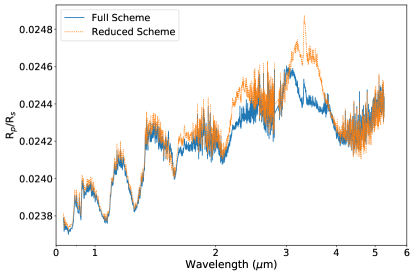
Figure 3: TauREx Forward models of HD 189733 b using parameters from Table 1.

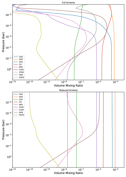
Figure 4: Vertical abundances profiles for the main constituents of HD 189733 b computed with FRECKLL using the Full Venot2020 scheme (top) and the Reduced Venot2020 scheme (bottom). Planetary and star parameters used are from Table 1.

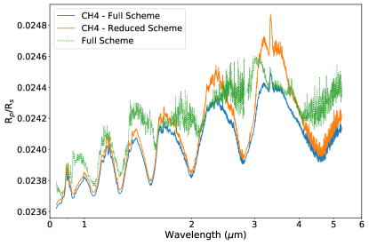
Figure 5: Contribution of methane to the spectra of HD 189733 b for both full and reduced schemes using parameters from Table 1.

From the chemistry predictions, we observe large differences between the two chemical schemes. In particular, while the predictions at the bottom of the atmospheres are consistent, large differences in the predicted abundances can be seen for the top of the atmosphere (below 0.1 bar). Those differences are likely due to the inclusion of reactions for photo-chemistry in the full scheme. We note, in particular, that the abundances of CH₄ and NH₃ decrease very rapidly for pressures above 10^-3 bar, while the C₂H₂ profile is significantly affected. This translates in large differences in the observed spectrum at the wavelengths that are probing those altitudes. For instance, the 2.3$\mu$m and 3.6$\mu$m methane features in Figure 3 and highlighted in Figure 5 are muted in the full scheme scenario as its strongly photolysed in the upper atmosphere, with differences of the order of 200ppm. Given the size of these features, and that these wavelength regions are covered by facilities such as JWST (Gardner et al., 2006), Twinkle (Edwards et al., 2019) and Ariel (Tinetti et al., 2018, 2021), these differences should be observable.

4 Retrievals

Parameter	Prior	Range
$R_{p}$	Uniform	0.8–2.0 $R_{J}$
$T$	Uniform	700.0–2500 K
$Z$	log-Uniform	10-1–$10^{3}$ $Z_{\odot}$
C/O	Uniform	0.1–2.0
$K_{zz}$	log-Uniform	103–1013 cm2/s

Table 2: Retrieval priors and ranges. The log prefix describes fitting the ranges in log-space

We now examine the viability of using a chemical kinetic solver in the context of retrievals and evaluate the biases introduced by the use of a reduced scheme or the assumption of chemical equilibrium. To our knowledge, this is the first time a full disequilibrium kinetic retrieval including vertical mixing and photo-chemistry is attempted. Due to the large number of samples evaluated in atmospheric retrievals, numerical stability across the full range of parameters explored is key, highlighting the importance of the improvements described in the Methodology section. We now use the forward model employing the full scheme from the previous section to simulate the observations. The high resolution spectrum is convolved with the JWST instrument response for one observation of HD 189733 b with NIRISS GR700XD and one with NIRSpec G395M. The error bars are obtained using the ExoWebb instrument simulator (Edwards et al., in prep), which is based upon the radiometric model from Edwards & Stotesbury (2021). Normally HD 189733 would saturate the NIRISS instrument which necessitates moving the star to 27 parsecs to prevent non-linearity in the detector response. The observed spectrum is shown in Figure 6.

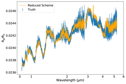
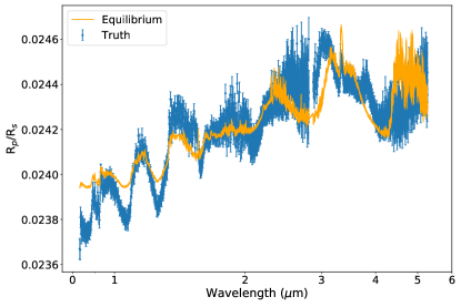
Figure 6: Simulated JWST observations of HD 189733 b (blue) with retrieval best-fit models (orange) for the full scheme (top panel), reduced scheme (bottom-left panel) and equilibrium (bottom-right).

We fit the JWST simulation using the full and reduced chemical networks as well as the equilibrium chemistry to evaluate the biases introduced by chemical assumptions. The results of these retrievals are shown in Figure 6. We utilize the same priors for all cases, which are described in Table 2. The $K_{zz}$ parameter, in particular, is fitted in the reduced and full schemes cases to uniform priors between $10^{3}$–$10^{12}$ cm².s^-1 inclusive in log-space. For benchmark purposes, and to provide comparisons with our previous works (Al-Refaie et al., 2021b, a), we highlight below the details of our hardware setup and computing use for this work. The retrievals performed in this work do not exploit GPU acceleration, which was introduced in Al-Refaie et al. (2021a), as the chemical kinetic solver is the dominant computational bottleneck. However, this allows us to mitigate the long computation time by exploiting large CPU-only nodes with significantly higher core counts. For our retrieval case, we use the DIRAC facility dedicating 180 cores per run. The retrievals utilised the MultiNest optimizer (Feroz et al., 2009; Buchner, 2016), with 750 live points and an evidence tolerance of 0.5 resulted in around 40,000 samples. The disequilibrium runs took 8 and 24 hours to complete for the reduced and full schemes, respectively. The equilibrium chemistry run took around 20 minutes.

Regarding the results of our retrievals with reduced and full schemes, the best-fit spectra are provided in Figure 6, the posteriors are provided in Figure 7 and the chemistry profiles are provided in Figure 8. From the inspection of the best-fit spectrum, we observe that, as expected, the full scheme matches the observations. Additionally, the recovered free parameters are close to the chosen true value (see Figure 7), and the recovered chemical profiles match the inputs within the uncertainties (see Figure 8). Notably, the $K_{zz}$ is well defined and retrieved accurately by the full scheme on the simulated JWST observations, implying that disequilibrium processes are observable with JWST. This was also shown in previous works (e.g. Greene et al., 2016; Blumenthal et al., 2018; Molaverdikhani et al., 2019; Drummond et al., 2020; Venot et al., 2020b).

For the reduced scheme, the best-fit spectrum is at most wavelengths able to reproduce the observations, but we observe large discrepancies at certain bands. For instance, the 3.6$\mu$m methane band is not well fitted by the reduced scheme, which, in our case, predicts too much methane. Due to the lack of flexibility and the assumptions introduced by self-consistent chemistry, the reduced scheme is likely unable to deduce the abundance of CH₄ without affecting the other important molecules of the atmosphere. This is confirmed in Figure 8. In most cases, the true value in this atmosphere is outside the 1$\sigma$ predictions of the reduced retrievals. The metallicity, for instance is found to be about Z = 6 when the input metallicity was solar (Z = 1). This is problematic as this could lead to incorrect interpretations, especially as such parameter is commonly used to link atmospheric composition to planetary formation (Öberg et al., 2011; Moses et al., 2013; Madhusudhan et al., 2016; Line et al., 2021).

Regarding the chemical equilibrium run, we find similar results. The retrieved parameters are most of the time outside the true values by more than 1$\sigma$. To compare the recovered metallicity again, assuming equilibrium chemistry it is found to be about Z = 32. In general, we find that using a chemical equilibrium assumption or a reduced scheme to recover the information content of a more complete full kinetic model that include photo-chemistry lead to strong biases. The recovered chemical profiles as seen in Figure 8 present large departures from the input with the main molecules being often different by more than two orders of magnitude. The predictions, for both equilibrium and reduced runs are overconfident and do not reflect the raw information content in the spectrum. This is due to the assumptions (equilibrium chemistry or pre-selected list of reactions) introduced in those models. This raises questions on the use of heavy assumptions in retrievals, such as equilibrium composition or reduced kinetic models (Changeat et al., 2019, 2020a; Al-Refaie et al., 2021a) or even one-dimensional retrievals (Feng et al., 2016; Caldas et al., 2019; Taylor et al., 2020; Changeat & Al-Refaie, 2020; MacDonald et al., 2020; Skaf et al., 2020; Pluriel et al., 2020).

5 Conclusion

We present FRECKLL a novel new code for fast computation and retrieval of chemical kinetics of exoplanet atmospheres. FRECKLL makes use of a distillation algorithm to significantly improve convergence to steady state. Using the FRECKLL and TauREx plugin we have successfully coupled chemical kinetics to a retrieval code and performed disequilibrium retrieval with a full kinetic model. We have shown that the use of strong assumptions about chemical composition (such as chemical equilibrium) or the use of reduced schemes could considerably bias the interpretation of observations.

6 Acknowledgments

This work utilised the OzSTAR national facility at Swinburne University of Technology. The OzSTAR program receives funding in part from the Astronomy National Collaborative Research Infrastructure Strategy (NCRIS) allocation provided by the Australian Government. This work utilised the Cambridge Service for Data Driven Discovery (CSD3), part of which is operated by the University of Cambridge Research Computing on behalf of the STFC DiRAC HPC Facility (www.dirac.ac.uk). The DiRAC component of CSD3 was funded by BEIS capital funding via STFC capital grants ST/P002307/1 and ST/R002452/1 and STFC operations grant ST/R00689X/1. DiRAC is part of the National e-Infrastructure.

A.A. and Q.C acknowledge funding from the European Research Council (ERC) under the European Union’s Horizon 2020 research and innovation programme (grant agreement No 758892, ExoAI), from the Science and Technology Funding Council grants ST/S002634/1 and ST/T001836/1 and from the UK Space Agency grant ST/W00254X/1.

Q.C. is the recipient of a 2022 European Space Agency Research Fellowship grant.

O.V. acknowledges funding from the ANR project ‘EXACT’ (ANR-21-CE49-0008-01), from the Centre National d’Études Spatiales (CNES), and from the CNRS/INSU Programme National de Planétologie (PNP).

BE is a Laureate of the Paris Region fellowship programme which is supported by the Ile-de-France Region and has received funding under the Horizon 2020 innovation framework programme and the Marie Sklodowska-Curie grant agreement no. 945298.

The authors wish to thank Alex Thompson and Sushuang Ma for brainstorming the name of this code.

7 Appendix 1: Posterior distributions for the simulated JWST spectrum

Figure 7 shows the posterior distributions for the simulated JWST retrievals.

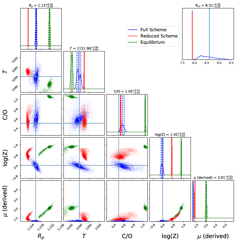
Figure 7: Posteriors from the retrieval of a simulated JWST spectra of HD 189733 b using full and reduced chemical network of Venot et al. (2020a) and equilibrium chemistry (Agúndez et al., 2012) with parameters given by Table 1. Blue and red are the posteriors using the full and reduced schemes with FRECKLL respectevly and green are the posteriors using equilibrium chemistry.

8 Appendix 2: Molecular profiles obtained in retrievals

Figure 8 shows the abundance profiles of the main chemical species in the retrievals.

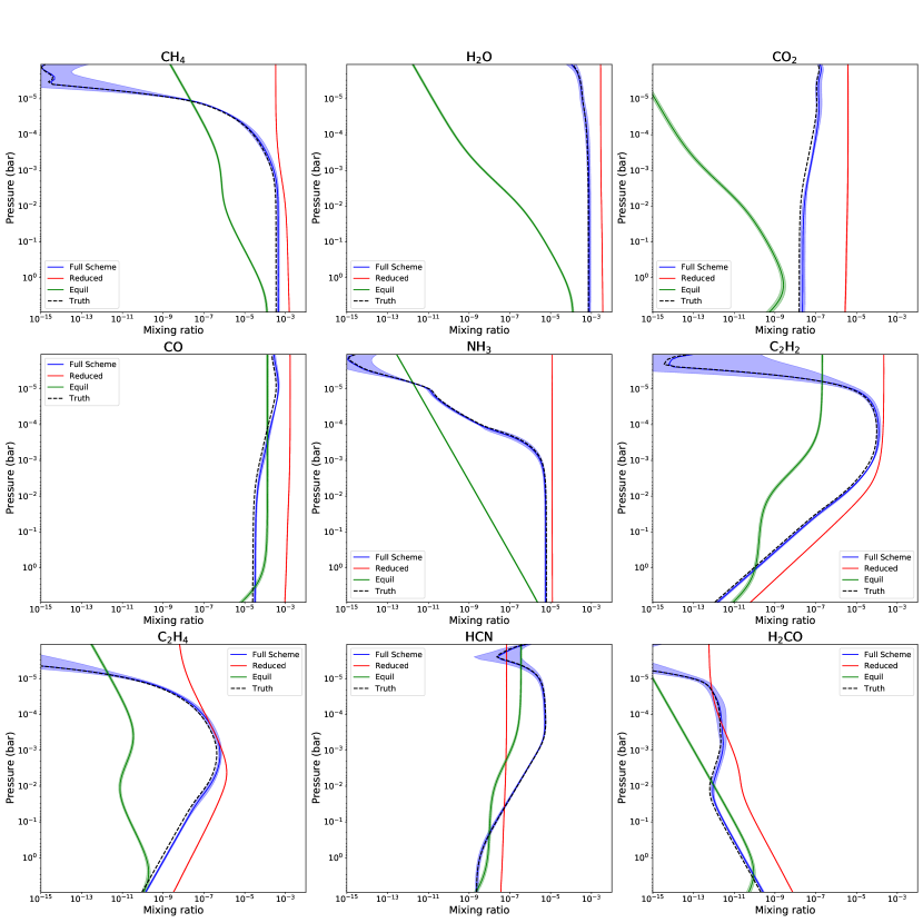
Figure 8: Chemical abundances profiles recovered by the reduced (red), full (blue) and equilibrium (green) retrievals in our simulations of HD 189733 b.

References

- Addison et al. (2019) Addison, B., Wright, D. J., Wittenmyer, R. A., et al. 2019, PASP, 131, 115003, doi: 10.1088/1538-3873/ab03aa
- Agúndez et al. (2012) Agúndez, M., Venot, O., Iro, N., et al. 2012, A&A, 548, A73, doi: 10.1051/0004-6361/201220365
- Al-Refaie et al. (2021a) Al-Refaie, A. F., Changeat, Q., Venot, O., Waldmann, I. P., & Tinetti, G. 2021a, arXiv e-prints, arXiv:2110.01271. https://arxiv.org/abs/2110.01271
- Al-Refaie et al. (2021b) Al-Refaie, A. F., Changeat, Q., Waldmann, I. P., & Tinetti, G. 2021b, ApJ, 917, 37, doi: 10.3847/1538-4357/ac0252
- Al-Refaie et al. (2015) Al-Refaie, A. F., Yachmenev, A., Tennyson, J., & Yurchenko, S. N. 2015, MNRAS, 448, 1704, doi: 10.1093/mnras/stv091
- Anisman et al. (2020) Anisman, L. O., Edwards, B., Changeat, Q., et al. 2020, AJ, 160, 233, doi: 10.3847/1538-3881/abb9b0
- Arcangeli et al. (2019) Arcangeli, J., Désert, J.-M., Parmentier, V., et al. 2019, A&A, 625, A136, doi: 10.1051/0004-6361/201834891
- Benneke & Seager (2012) Benneke, B., & Seager, S. 2012, ApJ, 753, 100, doi: 10.1088/0004-637X/753/2/100
- Blumenthal et al. (2018) Blumenthal, S. D., Mandell, A. M., Hébrard, E., et al. 2018, ApJ, 853, 138, doi: 10.3847/1538-4357/aa9e51
- Brown et al. (1989) Brown, P. N., Byrne, G. D., & Hindmarsh, A. C. 1989, SIAM Journal on Scientific and Statistical Computing, 10, 1038, doi: 10.1137/0910062
- Buchner (2016) Buchner, J. 2016, PyMultiNest: Python interface for MultiNest, Astrophysics Source Code Library, record ascl:1606.005. http://ascl.net/1606.005
- Caldas et al. (2019) Caldas, A., Leconte, J., Selsis, F., et al. 2019, A&A, 623, A161, doi: 10.1051/0004-6361/201834384
- Changeat (2022) Changeat, Q. 2022, AJ, 163, 106, doi: 10.3847/1538-3881/ac4475
- Changeat & Al-Refaie (2020) Changeat, Q., & Al-Refaie, A. 2020, ApJ, 898, 155, doi: 10.3847/1538-4357/ab9b82
- Changeat et al. (2020a) Changeat, Q., Al-Refaie, A., Mugnai, L. V., et al. 2020a, AJ, 160, 80, doi: 10.3847/1538-3881/ab9a53
- Changeat et al. (2021) Changeat, Q., Al-Refaie, A. F., Edwards, B., Waldmann, I. P., & Tinetti, G. 2021, ApJ, 913, 73, doi: 10.3847/1538-4357/abf2bb
- Changeat & Edwards (2021) Changeat, Q., & Edwards, B. 2021, ApJ, 907, L22, doi: 10.3847/2041-8213/abd84f
- Changeat et al. (2020b) Changeat, Q., Edwards, B., Al-Refaie, A. F., et al. 2020b, AJ, 160, 260, doi: 10.3847/1538-3881/abbe12
- Changeat et al. (2019) Changeat, Q., Edwards, B., Waldmann, I. P., & Tinetti, G. 2019, ApJ, 886, 39, doi: 10.3847/1538-4357/ab4a14
- Changeat et al. (2022) Changeat, Q., Edwards, B., Al-Refaie, A. F., et al. 2022, ApJS, 260, 3, doi: 10.3847/1538-4365/ac5cc2
- Chubb & Min (2022) Chubb, K. L., & Min, M. 2022, A&A, 665, A2, doi: 10.1051/0004-6361/202142800
- Chubb et al. (2020) Chubb, K. L., Tennyson, J., & Yurchenko, S. N. 2020, MNRAS, 493, 1531, doi: 10.1093/mnras/staa229
- Chubb et al. (2021) Chubb, K. L., Rocchetto, M., Yurchenko, S. N., et al. 2021, A&A, 646, A21, doi: 10.1051/0004-6361/202038350
- Coles et al. (2019) Coles, P. A., Yurchenko, S. N., & Tennyson, J. 2019, MNRAS, 490, 4638, doi: 10.1093/mnras/stz2778
- Crouzet et al. (2014) Crouzet, N., McCullough, P. R., Deming, D., & Madhusudhan, N. 2014, ApJ, 795, 166, doi: 10.1088/0004-637X/795/2/166
- Drummond et al. (2020) Drummond, B., Hébrard, E., Mayne, N. J., et al. 2020, A&A, 636, A68, doi: 10.1051/0004-6361/201937153
- Edwards et al. (in prep) Edwards, B., Mugnai, L., Al-Refaie, A., Changeat, Q., & Lagage, P.-O. in prep
- Edwards & Stotesbury (2021) Edwards, B., & Stotesbury, I. 2021, AJ, 161, 266, doi: 10.3847/1538-3881/abdf4d
- Edwards et al. (2019) Edwards, B., Rice, M., Zingales, T., et al. 2019, Experimental Astronomy, 47, 29, doi: 10.1007/s10686-018-9611-4
- Edwards et al. (2020) Edwards, B., Changeat, Q., Baeyens, R., et al. 2020, AJ, 160, 8, doi: 10.3847/1538-3881/ab9225
- Edwards et al. (2021) Edwards, B., Changeat, Q., Mori, M., et al. 2021, AJ, 161, 44, doi: 10.3847/1538-3881/abc6a5
- Eriksson et al. (1971) Eriksson, G., Holm, J. L., Welch, B. J., et al. 1971, Acta Chemica Scandinavica, 25, 2651
- Feng et al. (2016) Feng, Y. K., Line, M. R., Fortney, J. J., et al. 2016, ApJ, 829, 52, doi: 10.3847/0004-637X/829/1/52
- Feroz et al. (2009) Feroz, F., Hobson, M. P., & Bridges, M. 2009, MNRAS, 398, 1601, doi: 10.1111/j.1365-2966.2009.14548.x
- Fisher & Heng (2018) Fisher, C., & Heng, K. 2018, MNRAS, 481, 4698, doi: 10.1093/mnras/sty2550
- Fu et al. (2022) Fu, G., Sing, D. K., Deming, D., et al. 2022, AJ, 163, 190, doi: 10.3847/1538-3881/ac58fc
- Gardner et al. (2006) Gardner, J. P., Mather, J. C., Clampin, M., et al. 2006, Space Sci. Rev., 123, 485, doi: 10.1007/s11214-006-8315-7
- Greene et al. (2016) Greene, T. P., Line, M. R., Montero, C., et al. 2016, ApJ, 817, 17, doi: 10.3847/0004-637X/817/1/17
- Gressier et al. (2022) Gressier, A., Mori, M., Changeat, Q., et al. 2022, A&A, 658, A133, doi: 10.1051/0004-6361/202142140
- Harris et al. (2006) Harris, G. J., Tennyson, J., Kaminsky, B. M., Pavlenko, Y. V., & Jones, H. R. A. 2006, MNRAS, 367, 400, doi: 10.1111/j.1365-2966.2005.09960.x
- Haynes et al. (2015) Haynes, K., Mandell, A. M., Madhusudhan, N., Deming, D., & Knutson, H. 2015, ApJ, 806, 146, doi: 10.1088/0004-637X/806/2/146
- Hindmarsh (1983) Hindmarsh, A. 1983, IMACS Transactions on Scientific Computation, 1, 55
- Irwin et al. (2008) Irwin, P. G. J., Teanby, N. A., de Kok, R., et al. 2008, J. Quant. Spec. Radiat. Transf., 109, 1136, doi: 10.1016/j.jqsrt.2007.11.006
- Kahan (1987) Kahan, W. 1987, Unpublished manuscript, February
- Kreidberg et al. (2014) Kreidberg, L., Bean, J. L., Désert, J.-M., et al. 2014, Nature, 505, 69, doi: 10.1038/nature12888
- Li et al. (2015) Li, G., Gordon, I. E., Rothman, L. S., et al. 2015, ApJS, 216, 15, doi: 10.1088/0067-0049/216/1/15
- Line et al. (2014) Line, M. R., Knutson, H., Wolf, A. S., & Yung, Y. L. 2014, ApJ, 783, 70, doi: 10.1088/0004-637X/783/2/70
- Line et al. (2013) Line, M. R., Wolf, A. S., Zhang, X., et al. 2013, ApJ, 775, 137, doi: 10.1088/0004-637X/775/2/137
- Line et al. (2016) Line, M. R., Stevenson, K. B., Bean, J., et al. 2016, AJ, 152, 203, doi: 10.3847/0004-6256/152/6/203
- Line et al. (2021) Line, M. R., Brogi, M., Bean, J. L., et al. 2021, Nature, 598, 580, doi: 10.1038/s41586-021-03912-6
- MacDonald et al. (2020) MacDonald, R. J., Goyal, J. M., & Lewis, N. K. 2020, ApJ, 893, L43, doi: 10.3847/2041-8213/ab8238
- Madhusudhan et al. (2016) Madhusudhan, N., Agúndez, M., Moses, J. I., & Hu, Y. 2016, Space Sci. Rev., 205, 285, doi: 10.1007/s11214-016-0254-3
- Madhusudhan & Seager (2009) Madhusudhan, N., & Seager, S. 2009, ApJ, 707, 24, doi: 10.1088/0004-637X/707/1/24
- Mant et al. (2018) Mant, B. P., Yachmenev, A., Tennyson, J., & Yurchenko, S. N. 2018, MNRAS, 478, 3220, doi: 10.1093/mnras/sty1239
- Mikal-Evans et al. (2022) Mikal-Evans, T., Sing, D. K., Barstow, J. K., et al. 2022, Nature Astronomy, doi: 10.1038/s41550-021-01592-w
- Min et al. (2020) Min, M., Ormel, C. W., Chubb, K., Helling, C., & Kawashima, Y. 2020, A&A, 642, A28, doi: 10.1051/0004-6361/201937377
- Molaverdikhani et al. (2019) Molaverdikhani, K., Henning, T., & Mollière, P. 2019, ApJ, 883, 194, doi: 10.3847/1538-4357/ab3e30
- Mollière et al. (2019) Mollière, P., Wardenier, J. P., van Boekel, R., et al. 2019, A&A, 627, A67, doi: 10.1051/0004-6361/201935470
- Moses et al. (2013) Moses, J. I., Madhusudhan, N., Visscher, C., & Freedman, R. S. 2013, ApJ, 763, 25, doi: 10.1088/0004-637X/763/1/25
- Moses et al. (2011) Moses, J. I., Visscher, C., Fortney, J. J., et al. 2011, ApJ, 737, 15, doi: 10.1088/0004-637X/737/1/15
- Moses et al. (2016) Moses, J. I., Marley, M. S., Zahnle, K., et al. 2016, ApJ, 829, 66, doi: 10.3847/0004-637X/829/2/66
- Öberg et al. (2011) Öberg, K. I., Murray-Clay, R., & Bergin, E. A. 2011, ApJ, 743, L16, doi: 10.1088/2041-8205/743/1/L16
- Ogita et al. (2005) Ogita, T., Rump, S. M., & Oishi, S. 2005, SIAM Journal on Scientific Computing, 26, 1955, doi: 10.1137/030601818
- Pluriel et al. (2020) Pluriel, W., Zingales, T., Leconte, J., & Parmentier, V. 2020, A&A, 636, A66, doi: 10.1051/0004-6361/202037678
- Polyansky et al. (2018) Polyansky, O. L., Kyuberis, A. A., Zobov, N. F., et al. 2018, MNRAS, 480, 2597, doi: 10.1093/mnras/sty1877
- Saba et al. (2022) Saba, A., Tsiaras, A., Morvan, M., et al. 2022, AJ, 164, 2, doi: 10.3847/1538-3881/ac6c01
- Sedaghati et al. (2017) Sedaghati, E., Boffin, H. M. J., MacDonald, R. J., et al. 2017, Nature, 549, 238, doi: 10.1038/nature23651
- Sing et al. (2016) Sing, D. K., Fortney, J. J., Nikolov, N., et al. 2016, Nature, 529, 59, doi: 10.1038/nature16068
- Skaf et al. (2020) Skaf, N., Bieger, M. F., Edwards, B., et al. 2020, AJ, 160, 109, doi: 10.3847/1538-3881/ab94a3
- Stevenson et al. (2017) Stevenson, K. B., Line, M. R., Bean, J. L., et al. 2017, AJ, 153, 68, doi: 10.3847/1538-3881/153/2/68
- Swain et al. (2008) Swain, M. R., Bouwman, J., Akeson, R. L., Lawler, S., & Beichman, C. A. 2008, ApJ, 674, 482, doi: 10.1086/523832
- Taylor et al. (2020) Taylor, J., Parmentier, V., Irwin, P. G. J., et al. 2020, MNRAS, 493, 4342, doi: 10.1093/mnras/staa552
- Tennyson & Yurchenko (2012) Tennyson, J., & Yurchenko, S. N. 2012, MNRAS, 425, 21, doi: 10.1111/j.1365-2966.2012.21440.x
- Tennyson et al. (2020) Tennyson, J., Yurchenko, S. N., Al-Refaie, A. F., et al. 2020, J. Quant. Spec. Radiat. Transf., 255, 107228, doi: 10.1016/j.jqsrt.2020.107228
- The JWST Transiting Exoplanet Community Early Release Science Team et al. (2022) The JWST Transiting Exoplanet Community Early Release Science Team, Ahrer, E.-M., Alderson, L., et al. 2022, arXiv e-prints, arXiv:2208.11692. https://arxiv.org/abs/2208.11692
- Tinetti et al. (2007) Tinetti, G., Vidal-Madjar, A., Liang, M.-C., et al. 2007, Nature, 448, 169, doi: 10.1038/nature06002
- Tinetti et al. (2018) Tinetti, G., Drossart, P., Eccleston, P., et al. 2018, Experimental Astronomy, 46, 135, doi: 10.1007/s10686-018-9598-x
- Tinetti et al. (2021) Tinetti, G., Eccleston, P., Haswell, C., et al. 2021, arXiv e-prints, arXiv:2104.04824. https://arxiv.org/abs/2104.04824
- Tsai et al. (2021) Tsai, S.-M., Malik, M., Kitzmann, D., et al. 2021, ApJ, 923, 264, doi: 10.3847/1538-4357/ac29bc
- Tsiaras et al. (2018) Tsiaras, A., Waldmann, I. P., Zingales, T., et al. 2018, AJ, 155, 156, doi: 10.3847/1538-3881/aaaf75
- Venot et al. (2014) Venot, O., Agúndez, M., Selsis, F., Tessenyi, M., & Iro, N. 2014, A&A, 562, A51, doi: 10.1051/0004-6361/201322485
- Venot et al. (2020a) Venot, O., Cavalié, T., Bounaceur, R., et al. 2020a, A&A, 634, A78, doi: 10.1051/0004-6361/201936697
- Venot et al. (2012) Venot, O., Hébrard, E., Agúndez, M., et al. 2012, A&A, 546, A43, doi: 10.1051/0004-6361/201219310
- Venot et al. (2020b) Venot, O., Parmentier, V., Blecic, J., et al. 2020b, ApJ, 890, 176, doi: 10.3847/1538-4357/ab6a94
- Wakeford et al. (2017) Wakeford, H. R., Sing, D. K., Kataria, T., et al. 2017, Science, 356, 628, doi: 10.1126/science.aah4668
- Waldmann et al. (2015) Waldmann, I. P., Tinetti, G., Rocchetto, M., et al. 2015, ApJ, 802, 107, doi: 10.1088/0004-637X/802/2/107
- White et al. (1958) White, W. B., Johnson, S. M., & Dantzig, G. B. 1958, J. Chem. Phys., 28, 751, doi: 10.1063/1.1744264
- Wong et al. (2022) Wong, I., Chachan, Y., Knutson, H. A., et al. 2022, AJ, 164, 30, doi: 10.3847/1538-3881/ac7234
- Yurchenko et al. (2020) Yurchenko, S. N., Mellor, T. M., Freedman, R. S., & Tennyson, J. 2020, MNRAS, 496, 5282, doi: 10.1093/mnras/staa1874
- Yurchenko & Tennyson (2014) Yurchenko, S. N., & Tennyson, J. 2014, MNRAS, 440, 1649, doi: 10.1093/mnras/stu326