On the static effective Lindbladian of the squeezed Kerr oscillator

Abstract

We derive the static effective Lindbladian beyond the rotating wave approximation (RWA) for a driven nonlinear oscillator coupled to a bath of harmonic oscillators. The associated dissipative effects may explain orders of magnitude differences between the predictions of the ordinary RWA model and results from recent superconducting circuits experiments on the Kerr-cat qubit. The higher-order dissipators found in our calculations have important consequences for quantum error-correction protocols and parametric processses.

Introduction

Static effective Hamiltonians can be engineered in circuit quantum electrodynamics Blais et al. (2021) by coherently driving parametric processes. Such technique has been put to use in creating qubits Leghtas et al. (2015); Wang et al. (2016); Lescanne et al. (2020); Puri et al. (2017), gates between them Kurpiers et al. (2018); Axline et al. (2018); Rosenblum et al. (2018); Gao et al. (2018), readout schemes Krantz et al. (2016); Eddins et al. (2018); Touzard et al. (2019), and quantum simulations Kandala et al. (2017); Boettcher et al. (2020); Altman et al. (2021); Wang et al. (2020). Similar techniques are employed in quantum simulation with atomic systems Goldman and Dalibard (2014); Wintersperger et al. (2020); Martinez et al. (2016). Effective Hamiltonians resulting from complex pulse sequences in Trotterization schemes applied to a system Campagne-Ibarcq et al. (2020); Royer et al. (2020); Martinez et al. (2016); Eickbusch et al. (2021) can be also viewed as belonging to the above class.

Since physical systems are inevitably open, the nonlinear mixing processes associated with the Hamiltonian parametric terms of interest are also driven incoherently by fluctuations of the environment. These environmental fluctuations can be thermal in origin, in which case the process can be understood as a classical nonlinear mixing of noise that is down- or up-converted to the frequency of the nonlinear oscillator, or have an origin in the vacuum fluctuations of the environment. These vacuum fluctuations can be amplified by the drive and give rise to heating even in a zero temperature environment, a phenomenon known as Unruh heating when the driving force produces a simple time-independent acceleration Wilson et al. (2011); Blencowe and Wang (2020); Unruh (1976).

A recent work Petrescu et al. (2020) studied these effects in an attempt to explain drive-induced lifetime reduction in transmon circuits during readout. But in transmons, these effects tend to be masked by multiphoton nonlinear resonances limiting readout and parametric operations Sank et al. (2016); Blais et al. (2021); Shillito et al. (2022); Cohen et al. (2022). However, the recent implementation of a squeezed Kerr oscillator giving rise to the Kerr-cat qubit Puri et al. (2017); Grimm et al. (2020); Frattini et al. (2022) provides an ideal platform to uncover the effect of drive-enhanced environmental fluctuations, since unwanted nonlinear resonances of the transmon qubit are largely absent in this new system. Mixing of the environmental fluctuations is captured by beyond rotating wave approximation (RWA) in corrections to the system-bath coupling, giving rise to modified Lindbladian dynamics. In this note, we compute the static effective dissipators for the Kerr-cat system and discuss possible new effects that may explain experimental data in Frattini et al. (2022). Our systematic method, based on Venkatraman et al. (2022), can be extended to arbitrary order and can be applied to other controllable driven systems with a residual coupling to a bath.

Decoherence in a rapidly driven nonlinear system

The starting point of the calculation is the driven system-bath Hamiltonian

$$\hat{H}_{\mathrm{tot}}(t)=\hat{H}_{\mathrm{s}}+\hat{H}_{\mathrm{b}}+\hat{H}_{\mathrm{sb}}+\hat{H}_{\mathrm{d}}(t).$$ (1)

The system is a weakly nonlinear oscillator whose Hamiltonian is given by $\hat{H}_{\mathrm{s}}/\hbar=\omega_{o}\hat{a}^{\dagger}\hat{a}+\sum_{n}\frac{g_{n}}{n}\left(\hat{a}+\hat{a}^{\dagger}\right)^{n}.$ Here, $\hat{a}$ is the bosonic annihilation operator. The parameters $\omega_{o}$ and $g_{n}\ll\omega_{o}$ are the bare oscillator frequency and the $n$-th rank nonlinearity coefficients of the oscillator. We specialize our calculation to the case of the Josephson cosine potential as a source of oscillator nonlinearity and thus take the nonlinear coefficient $g_{n}$ of the Hamiltonian expansion to be of order $\varphi^{n-2}_{\mathrm{zps}}$ Venkatraman et al. (2022), where $\varphi_{\mathrm{zps}}$ is the zero point spread of the phase across the Josephson junction $\hat{\varphi}=\varphi_{\text{zps}}(\hat{a}+\hat{a}^{\dagger})$. The system is driven by $\hat{H}_{\mathrm{d}}(t)=-i\hbar F(t)\left(\hat{a}-\hat{a}^{\dagger}\right)$, where $F(t)$ is the waveform of the drive. At this time, we limit our analysis to the modeling of experiments in which the time dependence of the Hamiltonian corresponds to a monochromatic drive $F(t)=\Omega_{d}\cos(\omega_{d}t)$. The environment is taken to be a bath of linear oscillators with Hamiltonian $\hat{H}_{\mathrm{b}}=\sum_{j}\hbar\omega_{j}\hat{b}_{j}^{\dagger}\hat{b}_{j}$, which couples to the system by $\hat{H}_{\mathrm{sb}}=-\left(\hat{a}-\hat{a}^{\dagger}\right)\sum_{j}h_{j}\left(\hat{b}_{j}-\hat{b}_{j}^{\dagger}\right)$. In these expressions $\hat{b}_{j}$ is the annihilation operator of a bath mode at frequency $\omega_{j}$.

Motivated by the squeezed Kerr oscillator Wielinga and Milburn (1993); Cochrane et al. (1999); Puri et al. (2017, 2019); Grimm et al. (2020); Frattini et al. (2022); Chamberland et al. (2022); Roberts and Clerk (2020) and quantum information processing with cat-qubits Puri et al. (2017, 2019); Grimm et al. (2020); Leghtas et al. (2015); Lescanne et al. (2020); Putterman et al. (2022); Chamberland et al. (2022); Gautier et al. (2022); Kwon et al. (2022), we look now for the static effective description of $\hat{H}_{\text{tot}}$ under the condition $\omega_{d}\approx 2\omega_{o}$. The construction of this effective description involves successive unitary transformations followed by averaging out the fast oscillation terms in the new frame. First, following Venkatraman et al. (2022), we rewrite $\hat{H}_{\text{tot}}$ in a new frame comprising of (i) a displaced frame relative to the linear resonance of the oscillator to the drive so that
$\hat{a}\rightarrow\hat{a}+\frac{i\Omega_{d}}{2(\omega_{d}-\omega_{o})}e^{-i\omega_{d}t}-\frac{i\Omega_{d}}{2(\omega_{d}+\omega_{o})}e^{i\omega_{d}t}$, (ii) a rotating frame of $\hat{a}$ mode at $\omega_{d}/2$ so that $\hat{a}\rightarrow\hat{a}e^{-i\omega_{d}t/2}$, and then (iii) a rotating frame of each $\hat{b}_{j}$ mode at frequency $\omega_{j}$ so that $\hat{b}_{j}\rightarrow\hat{b}_{j}e^{-i\omega_{j}t}$. The Hamiltonian now reads

$$\hat{H}_{\text{tot}}=\hat{H}_{\mathrm{s}}(t)+\hat{H}_{\mathrm{sb}}(t)$$ (2a)

$$\begin{split}&\hat{{H}}_{\mathrm{s}}(t)/\hbar=\delta\hat{a}^{\dagger}\hat{a}+\sum_{n}\frac{g_{n}}{n}\Big{(}\hat{a}e^{-i\omega_{d}t/2}+\hat{a}^{\dagger}e^{i\omega_{d}t/2}\\ &\qquad\qquad\qquad\qquad\qquad\quad+\Pi e^{-i\omega_{d}t}+\Pi^{*}e^{i\omega_{d}t}\Big{)}^{n}\end{split}$$ (2b)

$$\begin{split}&\hat{{H}}_{\mathrm{sb}}(t)=i\left(\hat{a}e^{-i\omega_{d}t/2}-\hat{a}^{\dagger}e^{i\omega_{d}t/2}\right)\hat{B}(t),\end{split}$$ (2c)

where $\delta=\omega_{o}-\omega_{d}/2$, $\Pi\approx 4i\Omega_{d}/3\omega_{d}$, and $\hat{B}(t)=\sum_{j}ih_{\omega_{j}}\left(\hat{b}_{j}e^{-i\omega_{j}t}-\hat{b}_{j}^{\dagger}e^{i\omega_{j}t}\right)$. Averaging out the fast oscillation arising in $\hat{{H}}_{\mathrm{s}}(t)$, one finds the system Hamiltonian and its coupling to the environment under the RWA (order $\varphi_{\text{zps}}^{0}$). We further replace the sum $\sum_{j}$ over the bath modes with an integral introducing a density of modes $\lambda_{\omega}$ such that $\lambda_{\omega}d\omega$ gives the number of oscillators with frequencies in the interval from $\omega$ to $\omega+d\omega$. Tracing out the environment at this point under the usual Born-Markov approximation in a thermal bath provides the ordinary Lindbladian Gautier et al. (2022); Putterman et al. (2022); Chamberland et al. (2022), which involves the usual dissipators corresponding to single photon loss $\mathcal{D}[\hat{a}]$ and gain $\mathcal{D}[\hat{a}^{\dagger}]$ Carmichael (1999); Breuer et al. (2002), where $\mathcal{D}[\hat{O}]\bullet:=\hat{O}\bullet\hat{O}^{\dagger}-(\hat{O}^{\dagger}\hat{O}\bullet+\bullet\hat{O}^{\dagger}\hat{O})/2$. The effect of the bath under the Markov approximation is equivalent to a stochastic force coupled to the system by $i\hat{f}(t)(\hat{a}-\hat{a}^{\dagger})$ with spectral density $S_{f\!f}[\omega]=2\pi\lambda_{\omega}|h_{\omega}|^{2}\bar{n}_{\omega}$, $S_{f\!f}[-\omega]=2\pi\lambda_{\omega}|h_{\omega}|^{2}(1+\bar{n}_{\omega})$, where $\bar{n}_{\omega}$ is the average photon number of the mode $\hat{b}_{\omega}$ at frequency $\omega>0$ Clerk et al. (2010).

The key to obtaining our main result is to take into account terms beyond the RWA in the system-bath coupling and get an averaged description of $\hat{H}_{\mathrm{tot}}$. We follow our generalization of the Schrieffer-Wolff transformation procedure Venkatraman et al. (2022) to construct a near-identity canonical transformation generated by $\hat{S}(t)=\mathcal{O}(\varphi_{\text{zps}})$ so that the transformed Hamiltonian is time-independent to order $\varphi_{\text{zps}}^{k}$ for some arbitrarily large $k$ of interest. Under $\hat{S}$, $\hat{H}_{\mathrm{tot}}(t)\rightarrow\hat{{\mathcal{H}}}_{\mathrm{eff}}$, which is given as

$$\hat{\mathcal{H}}_{\mathrm{eff}} \equiv e^{\hat{S}/i\hbar}\hat{H}_{\mathrm{tot}}(t)e^{-\hat{S}/i\hbar}-i\hbar e^{\hat{S}/i\hbar}\partial_{t}e^{-\hat{S}/i\hbar}$$ (3)

$$=\hat{\mathcal{H}}_{\mathrm{s}}+\hat{\mathcal{H}}_{\mathrm{sb}},$$

where, by construction Venkatraman et al. (2022), $\hat{{\mathcal{H}}}_{\mathrm{eff}}$ is the static effective approximation of $\hat{H}_{\mathrm{tot}}(t)$, and the computation of $\hat{S}(t)$ is detailed in Appendix B. The first summand in Eq. 3 reads

$$\hat{\mathcal{H}}_{\mathrm{s}}/\hbar=\Delta\hat{a}^{\dagger}\hat{a}-K\hat{a}^{\dagger 2}\hat{a}^{2}+\epsilon_{2}(\hat{a}^{\dagger 2}+\hat{a}^{2})+\mathcal{O}(\varphi_{\mathrm{zps}}^{3}),$$ (4)

where $\Delta=\delta+6g_{4}|\Pi|^{2}-18g_{3}^{2}|\Pi|^{2}/\omega_{d}+2K$ is the Stark- and Lamb-shifted detuning, $K=-3g_{4}/2+20g_{3}^{2}/3\omega_{d}$ is the Kerr coefficient, and $\epsilon_{2}=g_{3}\Pi$ is the squeezing amplitude.

Effective Lindbladian at order $\varphi_{\text{zps}}^{1}$, i.e. first order beyond the RWA in the coupling to the environment

The canonical transformation generated by $\hat{S}(t)$ can be viewed as describing the system in an accelerated frame. In this frame, the system effectively experiences the static Hamiltonian Eq. 4; meanwhile, the system-bath coupling develops nonlinear components. Keeping terms to order $\varphi_{\mathrm{zps}}^{1}$, the perturbation parameter in the expansion of $\hat{S}(t)$, the system-environment coupling reads

$$\hat{\mathcal{H}}^{(1)}_{\mathrm{sb}}\approx{} i\left(\hat{a}e^{-i\omega_{d}t/2}-\hat{a}^{\dagger}e^{i\omega_{d}t/2}\right)\hat{B}(t)$$ (5)

$$+i\Big{(}-\frac{3\epsilon_{2}}{\omega_{d}}\hat{a}^{\dagger}e^{i3\omega_{d}t/2}-\frac{8g_{3}}{3\omega_{d}}\hat{a}^{\dagger 2}e^{i2\omega_{d}t/2}$$

$$-\frac{2\epsilon_{2}}{\omega_{d}}\hat{a}e^{i\omega_{d}t/2}+\frac{2\epsilon_{2}}{\omega_{d}}\hat{a}^{\dagger}e^{-i\omega_{d}t/2}$$

$$+\frac{8g_{3}}{\omega_{d}}\hat{a}^{2}e^{-i2\omega_{d}t/2}+\frac{3\epsilon_{2}}{\omega_{d}}\hat{a}e^{-i3\omega_{d}t/2}\Big{)}\hat{B}(t),$$

where the first line, at order $\varphi_{\text{zps}}^{0}$, is identical to the coupling term Eq. 2c.

Following a standard Lindbladian derivation Carmichael (1999, 2009); Breuer et al. (2002), but now with the renormalized system-bath Hamiltonian, we obtain the effective Lindblad master equation for the system up to order $\varphi^{1}_{\text{zps}}$ as

$$\begin{split}\partial_{t}\hat{\rho}_{s}=&\frac{1}{i\hbar}[\hat{\mathcal{H}}_{s},\hat{\rho}_{s}]+\kappa_{\omega_{d}/2}\bar{n}_{\omega_{d}/2}\mathcal{D}[\hat{a}^{\dagger}+\frac{2\epsilon_{2}}{\omega_{d}}\hat{a}]\hat{\rho}_{\mathrm{s}}\\ &+\kappa_{\omega_{d}/2}\left(1+\bar{n}_{\omega_{d}/2}\right)\mathcal{D}[\hat{a}+\frac{2\epsilon_{2}}{\omega_{d}}\hat{a}^{\dagger}]\hat{\rho}_{\mathrm{s}}\\ &+\kappa_{\omega_{d}}\bar{n}_{\omega_{d}}\left(\frac{8g_{3}}{3\omega_{d}}\right)^{2}\mathcal{D}\left[\hat{a}^{\dagger 2}\right]\hat{\rho}_{\mathrm{s}}\\ &+\kappa_{\omega_{d}}\left(1+\bar{n}_{\omega_{d}}\right)\left(\frac{8g_{3}}{3\omega_{d}}\right)^{2}\mathcal{D}\left[\hat{a}^{2}\right]\hat{\rho}_{\mathrm{s}}\\ &+\kappa_{3\omega_{d}/2}\bar{n}_{3\omega_{d}/2}\left(\frac{3\epsilon_{2}}{\omega_{d}}\right)^{2}\mathcal{D}\left[\hat{a}^{\dagger}\right]\hat{\rho}_{\mathrm{s}}\\ &+\kappa_{3\omega_{d}/2}\left(1+\bar{n}_{3\omega_{d}/2}\right)\left(\frac{3\epsilon_{2}}{\omega_{d}}\right)^{2}\mathcal{D}[\hat{a}]\hat{\rho}_{\mathrm{s}}.\end{split}$$ (6)

Here, $\kappa_{\omega}=2\pi\lambda_{\omega}|h_{\omega}|^{2}/\hbar^{2}=(S_{f\!f}[-\omega]-S_{f\!f}[\omega])/\hbar^{2}$ is the system-bath coupling rate at frequency $\omega$.

As our first observation, we note that one can expand the dissipator $\mathcal{D}[\hat{a}+\frac{2\epsilon_{2}}{\omega_{d}}\hat{a}^{\dagger}]$ in Eq. 6 to find a heating term that remains finite even at zero temperature: $\kappa_{\omega_{d}/2}\Big{(}\frac{2\epsilon_{2}}{\omega_{d}}\Big{)}^{2}\mathcal{D}[\hat{a}^{\dagger}]$. Its physical origin is a drive photon at frequency $\omega_{d}$ being converted to an oscillator excitation and an environment excitation, both at $\omega_{d}/2$. The associated effective Unruh-like temperature grows with the squeezing amplitude.

The dominant correction for the situation that interests us, however, is the parity-preserving two-photon heating term $\mathcal{D}[\hat{a}^{\dagger 2}]$. Its physical origin is in the thermal fluctuation at frequency $\omega_{d}$ driving incoherently the parametric process engineered to generate squeezing Grimm et al. (2020); Frattini et al. (2022).

With the Lindbladian at order $\varphi^{1}_{\text{zps}}$, we can compute the decoherence time $T_{X}$ of the ground coherent states (a.k.a Glauber states) of the system $\big{|}\alpha=\pm\sqrt{\epsilon_{2}/K}\big{\rangle}\approx|\pm X\big{\rangle}$, where $X$ stands for a Bloch sphere axis Grimm et al. (2020); Frattini et al. (2022). This quantity is the smallest non-zero real part of the Lindbladian eigenspectrum Albert and Jiang (2014); Frattini et al. (2022). In Fig. 1, we plot this quantity as a function of the squeezing amplitude. For our simulation parameters, we take $\kappa_{\omega_{d}}=5$ µs^-1 and temperature $T_{\omega_{d}}=350$ mK, which are reasonable values for a drive port considering standard couplings and the noise temperature of the electronics controlling the microwave signals in quantum circuit experiments. In addition, we choose $\kappa_{\omega_{d}/2}=\kappa_{3\omega_{d}/2}=0.05$ µs^-1 and temperature $T_{\omega_{d}/2}=T_{3\omega_{d}/2}=50$ mK, which are also based on experimental conditions of interest for this note. The nonlinear coefficients are taken to be $g_{3}/6\pi=20$ MHz, $g_{4}/8\pi=280$ kHz, and consequently $K/2\pi=320$ kHz, which are standard values for the SNAIL transmon Frattini et al. (2018) used in the experiments Frattini et al. (2022). The drive frequency is $\omega_{d}/2\pi=12$ GHz and the renormalized detuning in Eq. 4 is taken to be $\Delta=0.$

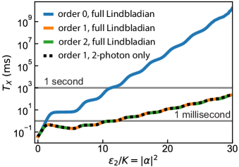
Figure 1: $T_{X}$ vs ${|\alpha|^{2}}$ for different orders of perturbation theory and realistic parameters. Theoretical predictions for the coherent state lifetime $T_{X}$ of the Kerr-cat qubit to order $\varphi^{0}_{\mathrm{zps}}$ in the coupling to the environment, corresponding to the ordinary Lindbladian treatment (containing only single photon loss and gain at $\omega=\omega_{d}/2$, blue), to order $\varphi^{1}_{\mathrm{zps}}$ in the coupling to the environment (orange), and to order $\varphi^{2}_{\mathrm{zps}}$ (green). Also shown is the effect of keeping only the two-photon terms at order $\varphi^{1}_{\mathrm{zps}}$ (see Eq. 7, black).

In Fig. 1, we show the Lindbladian prediction for the ordinary dissipators (order $\varphi^{0}_{\mathrm{zps}}$, blue) and that for dissipators to order $\varphi^{1}_{\mathrm{zps}}$ (orange). The two predictions disagree by several orders of magnitude, and thus the former, being incomplete, is unfit to describe state-of-the-art experiments Frattini et al. (2022). The prediction to order $\varphi^{2}_{\mathrm{zps}}$ (green), which we discuss in detail next, adds negligible corrections and shows the convergence of the method for the chosen parameter values. We note that the ratio of the prefactors of two-photon heating at order $\varphi_{\text{zps}}^{1}$ and single photon heating at order $\varphi_{\text{zps}}^{0}$ is $17~{}\mathrm{Hz}/12~{}\mathrm{Hz}\sim 1$. Yet the two-photon process becomes dominant for $\epsilon_{2}/K>2$ because its strength scales as $\langle(\hat{a}^{\dagger}\hat{a})^{2}\rangle\sim|\alpha|^{4}$ while that of the single photon process scales as $\langle\hat{a}^{\dagger}\hat{a}\rangle\sim|\alpha|^{2}$ . We also plot the Lindbladian prediction (black), computed from

$$\begin{split}\partial_{t}\hat{\rho}_{s}=&\frac{1}{i\hbar}[\hat{\mathcal{H}}_{s},\hat{\rho}_{s}]+\kappa_{\omega_{d}/2}\bar{n}_{\omega_{d}/2}\mathcal{D}[\hat{a}^{\dagger}]\hat{\rho}_{\mathrm{s}}\\ &+\kappa_{\omega_{d}/2}\left(1+\bar{n}_{\omega_{d}/2}\right)\mathcal{D}[\hat{a}]\hat{\rho}_{\mathrm{s}}\\ &+\kappa_{\omega_{d}}\bar{n}_{\omega_{d}}\left(\frac{8g_{3}}{3\omega_{d}}\right)^{2}\mathcal{D}\left[\hat{a}^{\dagger 2}\right]\hat{\rho}_{\mathrm{s}}\\ &+\kappa_{\omega_{d}}\left(1+\bar{n}_{\omega_{d}}\right)\left(\frac{8g_{3}}{3\omega_{d}}\right)^{2}\mathcal{D}\left[\hat{a}^{2}\right]\hat{\rho}_{\mathrm{s}},\end{split}$$ (7)

which only adds to the linear dissipators the term $\propto~{}\mathcal{D}[\hat{a}^{\dagger 2}]$ (and its conjugate). Its close similarity with the full Lindbladian prediction confirms that two-photon heating constitutes the dominant corrections to the ordinary Lindbladian. Note, though, that this decoherence process has only a marginal effect on the lifetime of large Schrödinger cat states ($\propto~{}|\alpha\rangle\pm|-\alpha\rangle$), since it conserves the parity of the state. Despite the failure of the ordinary Lindbladian to predict the lifetime of the coherent states, the lifetime of the Schrödinger cat states measured in Frattini et al. (2022) is still accounted for by the ordinary linear dissipation because of its inherent fragility to single photon loss events.

Effective Lindbladian at order $\varphi_{\text{zps}}^{2}$, i.e. second order beyond the RWA in the coupling to the environment

Similarly to the computation done at order $\varphi_{\text{zps}}^{1}$, we also compute $\hat{S}(t)$ generating the unitary transformation Eq. 3 to order $\varphi_{\text{zps}}^{2}$, as well as the effective Lindbladian to this order. The full expression is given in Eq. 15 in the appendix. The correction to this order may become relevant depending on the choice of parameters in the model, as we now discuss.

The second order Lindbladian samples the noise spectrum at $5\omega_{d}/2$, $2\omega_{d}$ and near zero frequency in addition to those sampled at the lower orders. For the noise spectrum at these frequencies, we chose $\kappa_{5\omega_{d}/2}=\kappa_{2\omega_{d}/2}=50$ ms^-1 and $T_{5\omega_{d}/2}=T_{2\omega_{d}}=50$ mK. For zero frequency, we take $\kappa_{0}=0$. These assignations were used also for the calculation to order $\varphi_{\text{zps}}^{2}$ in Fig. 1. We remark that the assignation for $\kappa_{0}$ is an important assumption, justified for the decoherence model proposed here. For a thermal bath of linear oscillators, the number of photons diverges near DC as $\bar{n}_{\text{th}}\sim k_{B}T/\hbar\omega$ while the density of modes (and thus $\kappa_{\omega}$) goes to zero as a polynomial in $\omega$ ($\propto\omega^{2}$ for a resistance coupled to the circuit by a capacitance). Thus, the noise spectral density at near-DC frequency goes to zero as $\omega\rightarrow 0$ in this model. However, for other noise models better suited to describe the low-frequency band including, for example quasi-particle loss and inductive loss Pop et al. (2014); Masluk (2013); Smith et al. (2020), the noise near DC could become dominant and Eq. 2c should also be extended to capture the corresponding coupling terms.

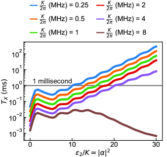
Figure 2: $T_{X}$ vs ${|\alpha|^{2}}$ for different Kerr nonlinearities. Theoretical predictions for the coherent state lifetime $T_{X}$ of the Kerr-cat qubit to order $\varphi_{\text{zps}}^{2}$ as a function of its mean photon number for several values of the Kerr constant $K$. The third rank nonlinearity is kept constant for all curves at $g_{3}/6\pi=20~{}\mathrm{MHz}$. The bath parameters are identical to Fig. 1. The brown curve corresponds to the prediction for parameters close to those in Grimm et al. (2020), whereas the blue curve corresponds to the prediction for parameters close to those in Frattini et al. (2022).

In Fig. 2, we show the effect of increasing the Kerr nonlinearity in the lifetime prediction at order $\varphi_{\text{zps}}^{2}$ while keeping the rank-three nonlinearity constant to $g_{3}/6\pi=20~{}\mathrm{MHz}$ as in Grimm et al. (2020); Frattini et al. (2022). The Kerr coefficient is varied by varying $g_{4}$ Frattini et al. (2018). The dominant dissipator appearing at this order is $\mathcal{D}[\hat{a}^{\dagger}\hat{a}]$, which on the coherent states acts as a single photon gain enhanced by a factor $|\alpha|^{2}$. The magnitude of this dissipator scales as $|K|^{4}|\Pi|^{2}\langle(\hat{a}^{\dagger}\hat{a})^{2}\rangle\propto|K|^{4}|\alpha|^{8}$ (see Eq. 15) and its prefactor ranges between $10^{-6}$ and $2$ times that of the dissipator $\mathcal{D}[\hat{a}^{\dagger 2}]$ at order $\varphi_{\text{zps}}^{1}$ when $K/2\pi$ is varied from 0.25 MHz to 8 MHz for a coherent state with $|\alpha|^{2}=20$. Consequently, this term becomes dominant for $K/2\pi>2$ MHz and for sufficiently large coherent state amplitudes. This is in qualitative agreement with the fact that the device in Grimm et al. (2020), characterized by $K/2\pi=6.7$ MHz, has a $T_{X}$ lifetime considerably lower than the one achieved in Frattini et al. (2022) where the device was operated at $K/2\pi=320$ kHz.

The main point of the exploration presented in this note is to showcase that an in-depth theoretical understanding of the dissipative processes at various orders is necessary for the experimental activity on parametric processes, like amplification, driven qubits, and quantum gates.

Comparison between theoretical predictions and experimental results

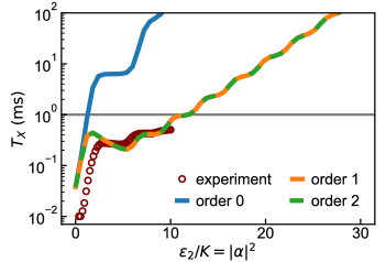
Figure 3: Experimental data and model. The experimental points correspond to the data in Frattini et al. (2022). The bath parameters in the model are identical to Fig. 1.

We have found that an ordinary Lindbladian treatment is incomplete by several orders of magnitude when the beyond-RWA terms are examined for the Kerr-cat qubit. Consequently, to account for experimental observations, higher orders in the Lindbladian need to be considered. With the analytical expression presented here, we are able to account for the order of magnitude of the observations presented in Frattini et al. (2022), which are reproduced as maroon dots in Fig. 3. Note that for $|\alpha|^{2}<2$, where there is a discrepancy between the experimental results and the predictions presented here, the data has been explained in Frattini et al. (2022), by the inclusion of non-Markovian low-frequency noise which is not included here. The results presented in this note emphasise the need for further experiments that will in turn lead to detailed modeling of possible noise sources affecting particularly driven qubits.

Acknowledgements

We acknowledge Alec Eickbusch, Daniel K. Weiss, Qile Su, Shruti Puri, and Steven M. Girvin for useful comments.

Appendix A Mitigating lifetime reduction by adding two-photon cooling

We identify that the dominant decoherence mechanisms are two-photon heating $\mathcal{D}[\hat{a}^{\dagger 2}]$ and dephasing $\mathcal{D}[\hat{a}^{\dagger}\hat{a}]\propto|\alpha|^{2}\mathcal{D}[\hat{a}^{\dagger}]$. To counteract this, we include, in our computation, a small amount of engineered two-photon dissipation Mirrahimi and Rouchon (2015); Leghtas et al. (2015); Puri et al. (2019); Lescanne et al. (2020); Doucet et al. (2020) ($\kappa_{\mathrm{2ph}}=0.003$ µs^-1). We show the outcome of the calculation in Fig. 4 for system and bath parameters as in Figs. 1 and 3. Experimentally, this should be easily achievable since much larger two-photon cooling rates have been demonstrated Touzard et al. (2019); Lescanne et al. (2020), albeit in absence of a Kerr nonlinearity. Note, however, that a correct understanding is likely to require a higher-order analysis of engineered dissipation Gautier et al. (2022); Putterman et al. (2022) like the one presented here. It is likely that the combination of Hamiltonian stabilization and reservoir engineering will provide the agility and fast universal gates for cat-qubits and high coherent state lifetimes Puri et al. (2019).

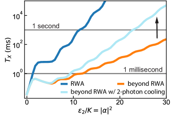
Figure 4: Effect of two-photon cooling. Adding an artificial two-photon dissipation term with a relatively small prefactor to the Kerr-cat system largely compensates the effect of the higher-order dissipators computed here. System and bath parameters have been chosen to be identical to those in Fig. 1.

Appendix B Static effective Hamiltonian

Here we follow Venkatraman et al. (2022) to compute $\hat{S}$ that generates the sought-after canonical transformation. First we expand Eq. 3 as

$$\hat{\mathcal{H}}_{\mathrm{eff}} \equiv e^{\hat{S}/i\hbar}\hat{H}_{\mathrm{tot}}(t)e^{-\hat{S}/i\hbar}-i\hbar e^{\hat{S}/i\hbar}\partial_{t}e^{-\hat{S}/i\hbar}$$ (8a)

$$\begin{split}&=\hat{{H}}_{\mathrm{s}}+\frac{1}{i\hbar}[\hat{S},\hat{{H}}_{\mathrm{s}}]+\frac{1}{2!(i\hbar)^{2}}[\hat{S},[\hat{S},\hat{{H}}_{\text{s}}]]+\cdots\\ &\quad+\hat{{H}}_{\mathrm{sb}}+\frac{1}{i\hbar}[\hat{S},\hat{{H}}_{\mathrm{sb}}]+\frac{1}{2!(i\hbar)^{2}}[\hat{S},[\hat{S},\hat{{H}}_{\text{sb}}]]+\cdots\\ &\quad+\partial_{t}\hat{S}+\frac{1}{2!i\hbar}[\hat{S},\partial_{t}{\hat{S}}]+\cdots\end{split}$$ (8b)

$$=\hat{\mathcal{H}}_{\mathrm{s}}+\hat{\mathcal{H}}_{\mathrm{sb}},$$ (8c)

where in LABEL:eq:supp-bch we have plugged in $\hat{{H}}_{\mathrm{tot}}=\hat{{H}}_{{s}}+\hat{{H}}_{\mathrm{sb}}$ as defined in Eq. 2 and employed the Baker-Campbell-Hausdorff formula; in Eq. 8c $\hat{\mathcal{H}}_{\mathrm{sb}}$ corresponds to the second line of LABEL:eq:supp-bch and $\hat{\mathcal{H}}_{\mathrm{s}}$ consists of the rest of LABEL:eq:supp-bch, which contains no bath modes.

Our goal is to perturbatively find $\hat{S}$ so that in the correponding frame $\hat{\mathcal{H}}_{\text{s}}$ is time-independent to some desired order of $\varphi_{\text{zps}}$. We therefore write $\hat{{H}}_{\mathrm{s}}$ and $\hat{S}$ each as a series

$$\hat{{H}}_{\mathrm{s}}=\sum_{k>0}\hat{{H}}_{\mathrm{s}}^{(k)},\quad\hat{S}=\sum_{k>0}\hat{S}^{(k)}$$ (9)

where $\hat{{H}}_{\mathrm{s}}^{(k)}$ and $\hat{S}^{(k)}$ are the order $\varphi_{\text{zps}}^{k}$ components in the corresponding series.

Demanding $\hat{\mathcal{H}}_{\text{s}}$ to be time-independent at order $\varphi_{\text{zps}}^{1}$ Venkatraman et al. (2022), we obtain the first order generator of the static effective transformation as

$$\frac{\hat{S}^{(1)}}{\hbar}=\; -\int dt\;\text{osc}\left(\hat{H}_{\text{s}}\right)$$ (10)

$$\begin{split}=\;&\frac{2}{5}i\frac{g_{3}}{\omega_{d}}a^{\dagger}\Pi^{*2}e^{i5\omega_{d}t/2}+\frac{1}{2}i\frac{g_{3}}{\omega_{d}}a^{\dagger 2}\Pi^{*}e^{i4\omega_{d}t/2}\\ &+\left(\frac{2}{3}i\frac{g_{3}}{\omega_{d}}a\Pi^{*2}+\frac{2}{9}i\frac{g_{3}}{\omega_{d}}a^{\dagger 3}\right)e^{i3\omega_{d}t/2}\\ &+2i\frac{g_{3}}{\omega_{d}}a^{\dagger}a\Pi^{*}e^{i2\omega_{d}t/2}\\ &+\Big{(}4i\frac{g_{3}}{\omega_{d}}|\Pi|^{2}a^{\dagger}+2i\frac{g_{3}}{\omega_{d}}a^{\dagger 2}a+2i\frac{g_{3}}{\omega_{d}}a^{\dagger}\Big{)}e^{i\omega_{d}t/2}\\ &+\text{h.c.}\end{split}$$ (11)

where $\text{osc}(f)=f-\int^{T}_{0}dt\;f$ extracts the oscillating part of $f$ with $T$ being its periodicity.

At this order, the transformed system-bath coupling is

$$\hat{\mathcal{H}}_{\mathrm{sb}}^{(1)}=\frac{[\hat{S}^{(1)},\hat{{H}}_{\mathrm{sb}}]}{i\hbar},$$ (12)

where $\hat{{H}}_{\mathrm{sb}}$ is taken to be of order $\varphi_{\text{zps}}^{0}$. Carrying out the calculation explicitly, one then obtains $\hat{\mathcal{H}}_{\mathrm{sb}}^{(1)}$ in Eq. 5.

At order $\varphi_{\text{zps}}^{2}$, the generator of the canonical transformation is accordingly given by

$$\frac{\hat{S}^{(2)}}{\hbar}\!=\!-\int_{0}^{t}dt\operatorname{osc}\!\Big{(}\hat{H}_{\text{s}}^{(2)}+\frac{[\hat{S}^{(1)},\hat{{H}}_{\mathrm{s}}^{(1)}]}{i\hbar}+\frac{[\hat{S}^{(1)},\partial_{t}{\hat{S}^{(1)}}]}{2!i\hbar}\Big{)},$$ (13)

the system-bath coupling is

$$\begin{split}\hat{{H}}_{\mathrm{sb}}^{(2)}&=\frac{1}{i\hbar}\left[S^{(2)},\hat{{H}}_{\mathrm{sb}}(t)\right]\\ &+\frac{1}{2!}\left(\frac{1}{i\hbar}\right)^{2}\left[S^{(1)},\left[S^{(1)},\hat{{H}}_{\mathrm{sb}}(t)\right]\right],\end{split}$$ (14)

and the full Lindbladian master equation up to this order is

$$\begin{split}\partial_{t}{\hat{\rho}_{\mathrm{s}}}&=\frac{1}{i\hbar}\left[\hat{\mathcal{H}}^{(2)}_{\mathrm{s}},\hat{\rho}_{\mathrm{s}}\right]+\kappa_{0}\left(1+\bar{n}_{0}\right)\mathcal{D}\left[32\frac{g_{3}^{2}}{\omega_{d}^{2}}a^{2}\Pi^{*}\right]+\kappa_{0}\bar{n}_{0}\ \mathcal{D}\left[32\frac{g_{3}^{2}}{\omega_{d}^{2}}a^{\dagger 2}\Pi\right]\\ &+\kappa_{\omega_{d}/2}\left(1+\bar{n}_{\omega_{d}/2}\right)\left(\mathcal{D}\left[a+\frac{2g_{3}}{\omega_{d}}a^{\dagger}\Pi-\left(\frac{35}{2}\frac{g_{3}^{2}}{\omega_{d}^{2}}-6\frac{g_{4}}{\omega_{d}}\right)a|\Pi|^{2}-\left({\frac{152}{9}}\frac{g_{3}^{2}}{\omega_{d}^{2}}-3\frac{g_{4}}{\omega_{d}}\right)a^{\dagger}a^{2}-\left({\frac{152}{9}}\frac{g_{3}^{2}}{\omega_{d}^{2}}-3\frac{g_{4}}{\omega_{d}}\right)a\right]\hat{\rho}_{\mathrm{s}}\right)\\ &+\kappa_{\omega_{d}/2}\bar{n}_{\omega_{d}/2}\left(\mathcal{D}\left[a^{\dagger}+\frac{2g_{3}}{\omega_{d}}a\Pi^{*}-\left(\frac{35}{2}\frac{g_{3}^{2}}{\omega_{d}^{2}}-6\frac{g_{4}}{\omega_{d}}\right)a^{\dagger}|\Pi|^{2}-\left(\frac{152}{9}\frac{g_{3}^{2}}{\omega_{d}^{2}}-3\frac{g_{4}}{\omega_{d}}\right)a^{\dagger 2}a-\left(\frac{152}{9}\frac{g_{3}^{2}}{\omega_{d}^{2}}-3\frac{g_{4}}{\omega_{d}}\right)a^{\dagger}\right]\hat{\rho}_{\mathrm{s}}\right)\\ &+\kappa_{\omega_{d}}\left(1+\bar{n}_{\omega_{d}}\right)\mathcal{D}\left[\frac{8g_{3}}{3\omega_{d}}a^{2}-\left(\frac{592}{9}\frac{g_{3}^{2}}{\omega_{d}^{2}}-16\frac{g_{4}}{\omega_{d}}\right)a^{\dagger}a\Pi\right]\hat{\rho}_{\mathrm{s}}\\ &+\kappa_{\omega_{d}}\bar{n}_{\omega_{d}}\mathcal{D}\left[\frac{8g_{3}}{3\omega_{d}}a^{\dagger 2}-\left(\frac{592}{9}\frac{g_{3}^{2}}{\omega_{d}^{2}}-16\frac{g_{4}}{\omega_{d}}\right)a^{\dagger}a\Pi^{*}\right]\hat{\rho}_{\mathrm{s}}\\ &+\kappa_{3\omega_{d}/2}\left(1+\bar{n}_{3\omega_{d}/2}\right)\mathcal{D}\left[\frac{3g_{3}}{\omega_{d}}a\Pi-\left(\frac{51}{5}\frac{g_{3}^{2}}{\omega_{d}^{2}}-\frac{9}{2}\frac{g_{4}}{\omega_{d}}\right)a^{\dagger}\Pi^{2}+\left(4\frac{g_{3}^{2}}{\omega_{d}^{2}}+\frac{3}{2}\frac{g_{4}}{\omega_{d}}\right)a^{3}\right]\hat{\rho}_{\mathrm{s}}\\ &+\kappa_{3\omega_{d}/2}\bar{n}_{3\omega_{d}/2}\mathcal{D}\left[\frac{3g_{3}}{\omega_{d}}a^{\dagger}\Pi^{*}-\left(\frac{51}{5}\frac{g_{3}^{2}}{\omega_{d}^{2}}-\frac{9}{2}\frac{g_{4}}{\omega_{d}}\right)a\Pi^{*2}+\left(4\frac{g_{3}^{2}}{\omega_{d}^{2}}+\frac{3}{2}\frac{g_{4}}{\omega_{d}}\right)a^{\dagger 3}\right]\hat{\rho}_{\mathrm{s}}\\ &+\kappa_{2\omega_{d}}\left(1+\bar{n}_{2\omega_{d}}\right)\mathcal{D}\left[\left(\frac{224}{45}\frac{g_{3}^{2}}{\omega_{d}^{2}}+\frac{16}{5}\frac{g_{4}}{\omega_{d}}\right)a^{2}\right]\hat{\rho}_{\mathrm{s}}\\ &+\kappa_{2\omega_{d}}\bar{n}_{2\omega_{d}}\mathcal{D}\left[\left(\frac{224}{45}\frac{g_{3}^{2}}{\omega_{d}^{2}}+\frac{16}{5}\frac{g_{4}}{\omega_{d}}\right)a^{\dagger 2}\right]\hat{\rho}_{\mathrm{s}}\\ &+\kappa_{5\omega_{d}/2}\left(1+\bar{n}_{5\omega_{d}/2}\right)\mathcal{D}\left[\left(\frac{19}{9}\frac{g_{3}^{2}}{\omega_{d}^{2}}+\frac{5}{2}\frac{g_{4}}{\omega_{d}}\right)a^{2}\right]\hat{\rho}_{\mathrm{s}}\\ &+\kappa_{5\omega_{d}/2}\bar{n}_{5\omega_{d}/2}\mathcal{D}\left[\left(\frac{19}{9}\frac{g_{3}^{2}}{\omega_{d}^{2}}+\frac{5}{2}\frac{g_{4}}{\omega_{d}}\right)a^{\dagger 2}\right]\hat{\rho}_{\mathrm{s}}.\end{split}$$ (15)

One can also obtain the photon-number-dependence and Kerr-dependence of relevant terms above using the relationship $g_{3}\Pi=K|\alpha|^{2}$ and $K=-3g_{4}/2+20g_{3}^{2}/3\omega_{d}$. With this, one sees that the prefactor of $\mathcal{D}[\hat{a}^{\dagger}\hat{a}]$ at frequency $\omega_{d}$ is $\propto|K|^{4}$. Such strong dependence on $K$ explains the drastic drop in $T_{X}$ for $K/2\pi>2$ MHz in Fig. 2, while for $K/2\pi<2$ MHz, the effect of $\mathcal{D}[\hat{a}^{\dagger}\hat{a}]$, which is of order $\varphi_{\text{zps}}^{2}$, is much weaker than the effect of dissipators at lower orders and thus the change of the former is masked by that of the latter when $K$ varies in this regime. Note that by engineering the Hamiltonian nonlinearities $g_{3}$ and $g_{4}$, one may be able to mitigate the effect of these dissipators even for a system with large $K$.

Appendix C Future directions and refinement of the model

When deriving the effective Lindbladian, we have made a few important assumptions.

First, we note that we use the usual Born approximation which amounts to assuming $h_{j}\ll\omega_{o}\varphi_{\text{zps}}^{2}$. This is, the Born approximation induces an error $\mathcal{O}(h_{j})$ which needs to remain much smaller than the perturbative corrections computed, which are of order $\varphi_{\text{zps}}^{2}$ in this work. Under the same assumption, we demand the transformed system-bath Hamiltonian $\hat{\mathcal{H}}_{\text{eff}}=\hat{\mathcal{H}}_{\text{s}}+\hat{\mathcal{H}}_{\text{sb}}$ to be static to order $\varphi_{\text{zps}}^{2}$. But since $\hat{\mathcal{H}}_{\text{sb}}=\mathcal{O}(h_{j})$, this amounts to demand that only $\hat{\mathcal{H}}_{\text{s}}$ be static, which provides an important but nonessential simplification.

We also remark that, in the standard Born-Markov approximation Carmichael (1999), one treats the system-bath coupling term in the interaction picture, i.e. $\exp({-\mathcal{\hat{H}}_{\text{s}}/i\hbar})\mathcal{\hat{H}}_{\text{sb}}\exp({\mathcal{\hat{H}}_{\text{s}}/i\hbar})$, instead of $\mathcal{\hat{H}}_{\text{sb}}$ as we did in this work. The omission of this frame transformation is valid under the assumption that the bath is white in the neighbourhood of any given frequency $\omega_{j}$ with a width of a few $K$’s wide covering the relevant portion of the spectrum of $\hat{\mathcal{H}}_{\text{s}}$. This assumption holds generally for $\omega_{j}\gg K$ Carmichael (1999, 2009), but should be dealt with delicately for the near-DC noise, which may be treated numerically. Specifically, one can numerically compute the DC system-bath coupling in the interaction picture defined by $\hat{\mathcal{H}}_{s}$ in Eq. 4. This will transform the DC system-bath coupling to a sum of near-DC terms. One can subsequently trace out the bath under the Born-Markov approximation and obtain the effective Lindbladian.

References

• Blais et al. (2021) A. Blais, A. L. Grimsmo, S. M. Girvin, and A. Wallraff, Reviews of Modern Physics 93, 025005 (2021).
• Leghtas et al. (2015) Z. Leghtas, S. Touzard, I. M. Pop, A. Kou, B. Vlastakis, A. Petrenko, K. M. Sliwa, A. Narla, S. Shankar, M. J. Hatridge, et al., Science 347, 853 (2015).
• Wang et al. (2016) C. Wang, Y. Y. Gao, P. Reinhold, R. W. Heeres, N. Ofek, K. Chou, C. Axline, M. Reagor, J. Blumoff, K. M. Sliwa, et al., Science 352, 1087 (2016).
• Lescanne et al. (2020) R. Lescanne, M. Villiers, T. Peronnin, A. Sarlette, M. Delbecq, B. Huard, T. Kontos, M. Mirrahimi, and Z. Leghtas, Nature Physics 16, 509 (2020).
• Puri et al. (2017) S. Puri, S. Boutin, and A. Blais, npj Quantum Information 3, 1 (2017).
• Kurpiers et al. (2018) P. Kurpiers, P. Magnard, T. Walter, B. Royer, M. Pechal, J. Heinsoo, Y. Salathé, A. Akin, S. Storz, J.-C. Besse, et al., Nature 558, 264 (2018), ISSN 1476-4687, URL https://doi.org/10.1038/s41586-018-0195-y.
• Axline et al. (2018) C. J. Axline, L. D. Burkhart, W. Pfaff, M. Zhang, K. Chou, P. Campagne-Ibarcq, P. Reinhold, L. Frunzio, S. M. Girvin, L. Jiang, et al., Nature Physics 14, 705 (2018), ISSN 1745-2481, URL https://doi.org/10.1038/s41567-018-0115-y.
• Rosenblum et al. (2018) S. Rosenblum, Y. Y. Gao, P. Reinhold, C. Wang, C. J. Axline, L. Frunzio, S. M. Girvin, L. Jiang, M. Mirrahimi, M. H. Devoret, et al., Nature Communications 9, 652 (2018), ISSN 2041-1723, URL https://doi.org/10.1038/s41467-018-03059-5.
• Gao et al. (2018) Y. Y. Gao, B. J. Lester, Y. Zhang, C. Wang, S. Rosenblum, L. Frunzio, L. Jiang, S. M. Girvin, and R. J. Schoelkopf, Phys. Rev. X 8, 021073 (2018), URL https://link.aps.org/doi/10.1103/PhysRevX.8.021073.
• Krantz et al. (2016) P. Krantz, A. Bengtsson, M. Simoen, S. Gustavsson, V. Shumeiko, W. Oliver, C. Wilson, P. Delsing, and J. Bylander, Nature communications 7, 1 (2016).
• Eddins et al. (2018) A. Eddins, S. Schreppler, D. M. Toyli, L. S. Martin, S. Hacohen-Gourgy, L. C. G. Govia, H. Ribeiro, A. A. Clerk, and I. Siddiqi, Phys. Rev. Lett. 120, 040505 (2018), URL https://link.aps.org/doi/10.1103/PhysRevLett.120.040505.
• Touzard et al. (2019) S. Touzard, A. Kou, N. E. Frattini, V. V. Sivak, S. Puri, A. Grimm, L. Frunzio, S. Shankar, and M. H. Devoret, Phys. Rev. Lett. 122, 080502 (2019), URL https://link.aps.org/doi/10.1103/PhysRevLett.122.080502.
• Kandala et al. (2017) A. Kandala, A. Mezzacapo, K. Temme, M. Takita, M. Brink, J. M. Chow, and J. M. Gambetta, Nature 549, 242 (2017).
• Boettcher et al. (2020) I. Boettcher, P. Bienias, R. Belyansky, A. J. Kollár, and A. V. Gorshkov, Phys. Rev. A 102, 032208 (2020), URL https://link.aps.org/doi/10.1103/PhysRevA.102.032208.
• Altman et al. (2021) E. Altman, K. R. Brown, G. Carleo, L. D. Carr, E. Demler, C. Chin, B. DeMarco, S. E. Economou, M. A. Eriksson, K.-M. C. Fu, et al., PRX Quantum 2, 017003 (2021), URL https://link.aps.org/doi/10.1103/PRXQuantum.2.017003.
• Wang et al. (2020) C. S. Wang, J. C. Curtis, B. J. Lester, Y. Zhang, Y. Y. Gao, J. Freeze, V. S. Batista, P. H. Vaccaro, I. L. Chuang, L. Frunzio, et al., Phys. Rev. X 10, 021060 (2020), URL https://link.aps.org/doi/10.1103/PhysRevX.10.021060.
• Goldman and Dalibard (2014) N. Goldman and J. Dalibard, Phys. Rev. X 4, 031027 (2014).
• Wintersperger et al. (2020) K. Wintersperger, C. Braun, F. N. Ünal, A. Eckardt, M. D. Liberto, N. Goldman, I. Bloch, and M. Aidelsburger, Nature Physics 16, 1058 (2020), ISSN 1745-2481, URL https://doi.org/10.1038/s41567-020-0949-y.
• Martinez et al. (2016) E. A. Martinez, C. A. Muschik, P. Schindler, D. Nigg, A. Erhard, M. Heyl, P. Hauke, M. Dalmonte, T. Monz, P. Zoller, et al., Nature 534, 516 (2016), ISSN 1476-4687, URL https://doi.org/10.1038/nature18318.
• Campagne-Ibarcq et al. (2020) P. Campagne-Ibarcq, A. Eickbusch, S. Touzard, E. Zalys-Geller, N. E. Frattini, V. V. Sivak, P. Reinhold, S. Puri, S. Shankar, R. J. Schoelkopf, et al., Nature 584, 368 (2020), ISSN 1476-4687, URL https://doi.org/10.1038/s41586-020-2603-3.
• Royer et al. (2020) B. Royer, S. Singh, and S. M. Girvin, Phys. Rev. Lett. 125, 260509 (2020), URL https://link.aps.org/doi/10.1103/PhysRevLett.125.260509.
• Eickbusch et al. (2021) A. Eickbusch, V. Sivak, A. Z. Ding, S. S. Elder, S. R. Jha, J. Venkatraman, B. Royer, S. M. Girvin, R. J. Schoelkopf, and M. H. Devoret, Fast universal control of an oscillator with weak dispersive coupling to a qubit (2021), URL https://arxiv.org/abs/2111.06414.
• Wilson et al. (2011) C. M. Wilson, G. Johansson, A. Pourkabirian, M. Simoen, J. R. Johansson, T. Duty, F. Nori, and P. Delsing, Nature 479, 376 (2011).
• Blencowe and Wang (2020) M. P. Blencowe and H. Wang, Philosophical Transactions of the Royal Society A: Mathematical, Physical and Engineering Sciences 378, 20190224 (2020).
• Unruh (1976) W. G. Unruh, Phys. Rev. D 14, 870 (1976), URL https://link.aps.org/doi/10.1103/PhysRevD.14.870.
• Petrescu et al. (2020) A. Petrescu, M. Malekakhlagh, and H. E. Türeci, Physical Review B 101, 134510 (2020).
• Sank et al. (2016) D. Sank, Z. Chen, M. Khezri, J. Kelly, R. Barends, B. Campbell, Y. Chen, B. Chiaro, A. Dunsworth, A. Fowler, et al., Phys. Rev. Lett. 117, 190503 (2016), URL https://link.aps.org/doi/10.1103/PhysRevLett.117.190503.
• Shillito et al. (2022) R. Shillito, A. Petrescu, J. Cohen, J. Beall, M. Hauru, M. Ganahl, A. G. M. Lewis, G. Vidal, and A. Blais, Dynamics of transmon ionization (2022), URL https://arxiv.org/abs/2203.11235.
• Cohen et al. (2022) J. Cohen, A. Petrescu, R. Shillito, and A. Blais, Reminiscence of classical chaos in driven transmons (2022), URL https://arxiv.org/abs/2207.09361.
• Grimm et al. (2020) A. Grimm, N. E. Frattini, S. Puri, S. O. Mundhada, S. Touzard, M. Mirrahimi, S. M. Girvin, S. Shankar, and M. H. Devoret, Nature 584, 205 (2020).
• Frattini et al. (2022) N. E. Frattini, R. G. Cortiñas, J. Venkatraman, X. Xiao, Q. Su, C. U. Lei, B. J. Chapman, V. R. Joshi, S. M. Girvin, R. J. Schoelkopf, et al., The squeezed kerr oscillator: spectral kissing and phase-flip robustness (2022), URL https://arxiv.org/abs/2209.03934.
• Venkatraman et al. (2022) J. Venkatraman, X. Xiao, R. G. Cortiñas, A. Eickbusch, and M. H. Devoret, Phys. Rev. Lett. 129, 100601 (2022), URL https://link.aps.org/doi/10.1103/PhysRevLett.129.100601.
• Wielinga and Milburn (1993) B. Wielinga and G. J. Milburn, Phys. Rev. A 48, 2494 (1993), URL https://link.aps.org/doi/10.1103/PhysRevA.48.2494.
• Cochrane et al. (1999) P. T. Cochrane, G. J. Milburn, and W. J. Munro, Phys. Rev. A 59, 2631 (1999), URL https://link.aps.org/doi/10.1103/PhysRevA.59.2631.
• Puri et al. (2019) S. Puri, A. Grimm, P. Campagne-Ibarcq, A. Eickbusch, K. Noh, G. Roberts, L. Jiang, M. Mirrahimi, M. H. Devoret, and S. M. Girvin, Phys. Rev. X 9, 041009 (2019), URL https://link.aps.org/doi/10.1103/PhysRevX.9.041009.
• Chamberland et al. (2022) C. Chamberland, K. Noh, P. Arrangoiz-Arriola, E. T. Campbell, C. T. Hann, J. Iverson, H. Putterman, T. C. Bohdanowicz, S. T. Flammia, A. Keller, et al., PRX Quantum 3, 010329 (2022), URL https://link.aps.org/doi/10.1103/PRXQuantum.3.010329.
• Roberts and Clerk (2020) D. Roberts and A. A. Clerk, Physical Review X 10, 021022 (2020).
• Putterman et al. (2022) H. Putterman, J. Iverson, Q. Xu, L. Jiang, O. Painter, F. G. Brandão, and K. Noh, Physical Review Letters 128, 110502 (2022), publisher: American Physical Society, URL https://link.aps.org/doi/10.1103/PhysRevLett.128.110502.
• Gautier et al. (2022) R. Gautier, A. Sarlette, and M. Mirrahimi, arXiv:2112.05545 [quant-ph] (2022), arXiv: 2112.05545, URL http://arxiv.org/abs/2112.05545.
• Kwon et al. (2022) S. Kwon, S. Watabe, and J.-S. Tsai, npj Quantum Information 8, 40 (2022), ISSN 2056-6387, URL https://doi.org/10.1038/s41534-022-00553-z.
• Carmichael (1999) H. J. Carmichael, Statistical methods in quantum optics 1: master equations and Fokker-Planck equations, vol. 1 (Springer Science & Business Media, 1999).
• Breuer et al. (2002) H.-P. Breuer, F. Petruccione, et al., The theory of open quantum systems (Oxford University Press on Demand, 2002).
• Clerk et al. (2010) A. A. Clerk, M. H. Devoret, S. M. Girvin, F. Marquardt, and R. J. Schoelkopf, Reviews of Modern Physics 82, 1155 (2010).
• Carmichael (2009) H. J. Carmichael, Statistical methods in quantum optics 2: Non-classical fields (Springer Science & Business Media, 2009).
• Albert and Jiang (2014) V. V. Albert and L. Jiang, Physical Review A 89, 022118 (2014).
• Frattini et al. (2018) N. E. Frattini, V. V. Sivak, A. Lingenfelter, S. Shankar, and M. H. Devoret, Phys. Rev. Applied 10, 054020 (2018), URL https://link.aps.org/doi/10.1103/PhysRevApplied.10.054020.
• Pop et al. (2014) I. M. Pop, K. Geerlings, G. Catelani, R. J. Schoelkopf, L. I. Glazman, and M. H. Devoret, Nature 508, 369–372 (2014).
• Masluk (2013) N. A. Masluk, Reducing the losses of the fluxonium artificial atom (Yale University, 2013).
• Smith et al. (2020) W. C. Smith, A. Kou, X. Xiao, U. Vool, and M. H. Devoret, npj Quantum Information 6, 8 (2020), ISSN 2056-6387.
• Mirrahimi and Rouchon (2015) M. Mirrahimi and P. Rouchon, Dynamics and control of open quantum systems (2015).
• Doucet et al. (2020) E. Doucet, F. Reiter, L. Ranzani, and A. Kamal, Physical Review Research 2, 023370 (2020).