Massive Color-Kinematics Duality and Double-Copy
for Kaluza-Klein Scattering Amplitudes

Abstract

We study the structure of scattering amplitudes of massive Kaluza-Klein (KK) states under toroidal compactification. We present a shifting method to quantitatively derive the scattering amplitudes of massive KK gauge bosons and KK gravitons from the corresponding massless amplitudes in the noncompactified higher dimensional theories. With these we construct the massive KK scattering amplitudes by extending the double-copy relations of massless scattering amplitudes within the field theory framework, including both the BCJ and CHY methods, and build up their connections to the massive KK KLT relations. We present the massive BCJ-type double-copy construction of the $N$-point KK gauge boson/graviton scattering amplitudes, and as the applications we derive explicitly the four-point KK scattering amplitudes as well as the five-point KK scattering amplitudes. We further study the nonrelativistic limit of these massive scattering amplitudes with the heavy external KK states and discuss the impact of the compactified extra dimensions on the low energy gravitational potential. Finally, we analyze the four-point and $N$-point mass spectral conditions and newly propose a novel group theory approach to prove that only the KK theories under toroidal compactification can satisfy these conditions for directly realizing massive double-copy in the field theory framework.
JHEP (in press), [arXiv:2209.11191 [hep-th]].

1 Introduction

Scattering amplitude is an important means for studying fundamental forces in nature, and can bridge theories with experiments. One of the greatest challenges in modern physics is the unification of gravitational force with the gauge forces of electromagnetic, weak and strong interactions of all elementary particles. This leads to the explorations of a higher dimensional spacetime structure, with extra spatial dimensions compactified on the boundaries and being smaller than the existing observational limits. Such attempts started a century ago from the Kaluza-Klein (KK) theory for unifying the gravitational and electromagnetic forces with a compactified fifth dimension (5d) KK . This opened up a truly fundamental direction, and has been seriously pursued and extensively developed in various contexts, including the string/M theories string and the extra dimensional field theories with large or small extra dimensions Exd0 Exd ExdRS . The KK compactification predicts an infinite tower of massive KK excitations for each known particle of the Standard Model (SM). These have intrigued substantial phenomenological and experimental efforts over the past two decades to search for the low-lying KK states of the extra dimensional KK theories exdpheno exd-rev , which could produce the first signatures of new physics beyond the SM, including the KK states of gravitons and of the SM particles as well as the possible dark matter candidate.

The longstanding difficulty of unifying the gravitational force with the gauge forces arises from the intricate nonlinearity and perturbative nonrenormalizability of the Einstein theory of General Relativity (GR), in contrast to the modern renormalizable gauge theories of the electroweak and strong interactions in the SM of particle physics. However, the scattering amplitudes of gravitons and gauge bosons are connected through the conjectured deep relation of double-copy, $\hskip 0.85358pt\text{GR}\!=\!(\text{Gauge~{}Theory})^{2}\hskip 0.85358pt$, even though it does not manifest at the Lagrangian (Hamiltonian) level.  The double-copy relation points to the common fundamental root of both the gravity force and gauge forces. It has also become a powerful tool for efficiently computing the highly intricate scattering amplitudes of spin-2 gravitons. The massive KK graviton scattering amplitudes are especially involved (with large energy cancellations) Chivukula:2020 Kurt-2019 Hang:2021fmp and the $N$-point longitudinal KK graviton amplitudes have their leading energy dependence nontrivially cancelled down by a large power factor $\hskip 0.85358ptE^{2N}\!\!$ ($N\!\geqslant\!4$) up to any loop order Hang:2021fmp . The first double-copy was constructed by Kawai-Lewellen-Tye (KLT) KLT to link the scattering amplitudes of massless closed strings to the products of scattering amplitudes of massless open strings at tree level. The KLT relation leads to the connection between the scattering amplitudes of massless gravitons and the products of the color-ordered amplitudes of massless gauge bosons in the low energy field-theory limit. Then, Bern-Carrasco-Johansson (BCJ) constructed the double-copy within the field theory formalism through the color-kinematics duality BCJ:2008 BCJ:2019 , which connects the (squared) scattering amplitudes of massless gauge bosons to the corresponding massless graviton amplitudes. The massless double-copy relations of BCJ may be proven and refined by analyzing the tree-level scattering amplitudes of the massless heterotic strings and open strings Tye-2010 . They may also be proven BCJ:2019 by using the on-shell recursion relation of Britto-Cachazo-Feng-Witten (BCFW) BCFW and be extended to loop levels in the field theory framework. Afterwards, the worldsheet Cachazo-He-Yuan (CHY) method CHY was motivated by Witten’s twistor string theory Witten:2003nn , it further shows that the KLT kernel can be interpreted as the inverse amplitudes of bi-adjoint scalars; it can also extend the double-copy relations to other field theories than the gauge/gravity theories CHY14 . But, all these works were to formulate and test double-copy for the scattering amplitudes of massless gauge bosons/gravitons BCJ:2019 . Our recent works extended the massless double-copy method to the massive double-copy constructions for the 5d KK gauge/gravity field theories (with orbifold compactification) Hang:2021fmp , for the compactified 26d KK bosonic string theory plus its field theory limit KKString , and for the 3d topologically massive Chern-Simons (CS) gauge/gravity theories Hang:2021oso . In the literatue, some other recent works attempted to generalize the massless double-copy method to the case of massive double-copies, including the 4d massive Yang-Mills (YM) theory versus Fierz-Pauli-like massive gravity dRGT DC-4dx1 , the spontaneously broken YM-Einstein supergravity models with adjoint Higgs fields SUGRAhiggs , the KK-inspired effective gauge theory with extra global U(1) Momeni:2020hmc , the 3d Chern-Simons (CS) gauge/gravity theories with or without supersymmetry 3dCS-susy 3dCS1 Gonzalez:2021bes , and certain massive scalar theories DC-scalar .

Extensions of the conventional massless double-copy formalism to the case of massive gauge/gravity theories are generally difficult, because many theories of this kind violate gauge symmetry and diffeomorphism invariance (which include the massive YM theory and the massive Fierz-Pauli gravity FP ). By adding extra non-linear polynomial interaction terms in the literature dRGT DC-4dx1 , one could realize the double-copy between the massive YM and Fierz-Pauli gravity theories, but the high energy behavior of the four-point massive graviton amplitudes could be improved to no better than $E^{6}$ Cheung2016 Kurt-E6 and is still much worse than the final energy-dependence of $O(E^{2})$ in the tree-level massive KK graviton scattering amplitudes Chivukula:2020 Kurt-2019 Hang:2021fmp . The KK compactification can realize a geometric “Higgs” mechanism for mass generation of KK gravitons both at the Lagrangian level GHiggs Hang:2021fmp and at the scattering $S$-matrix level Hang:2021fmp . This is shown Hang:2021fmp to make the massive KK GR theory free from the van-Dam-Veltman-Zakharov (vDVZ) discontinuity vDVZ and exhibit much better high energy behaviors (as good as that of the massless Einstein gravity). Hence the KK GR theories provide a truly consistent realization of the massive gravity in the effective field theory formulation. Another important realization of consistent massive double-copy is given by the 3d topologically massive Chern-Simons gauge and gravity theories TMG because they have topological mass-generations for the gauge bosons and gravitons in a gauge-invariant manner and guarantee the good high energy behaviors of the massive gauge boson/graviton scattering amplitudes Hang:2021oso .

Our recent works studied the massive double-copy constructions for the KK gauge/gravity field theories under the 5d compactification with the $S^{1}\!/\mathbb{Z}_{2}$ orbifold Hang:2021fmp , and for the 26d KK bosonic string theory under the compactification of $\mathbb{R}^{1,24}\otimes S^{1}$ KKString . We found Hang:2021fmp that the massive double-copy construction for the 5d KK theories with $S^{1}\!/\mathbb{Z}_{2}$ orbifold compactification is highly involved because the KK gauge boson scattering amplitudes exhibit double-pole structures and the naive extension of the conventional massless BCJ method does not work. By making the high energy expansion, we proved Hang:2021fmp that the leading order (LO) KK gauge boson amplitudes are mass-independent and obey the color-kinematics duality. So the massive double-copy works at the LO [which is enough for our double-copy construction of the KK Gravitational Equivalence Theorem (GRET) Hang:2021fmp ], but it does not exactly work at the next-to-leading-order (NLO) and beyond, unless certain special treatment is made. Then, by using the first principle approach of KK string theory, we realized KKString that the massive extension of the KLT-type double-copy construction could exactly work for the 5d $S^{1}$ compactification without orbifold  under which the KK amplitudes have single-pole structure, exhibit the massive color-kinematics duality, and obey the mass spectral condition. As the resolution for the nontrivial case of the orbifold compactification, we found KKString that the correct double-copied KK graviton amplitudes can be constructed in terms of proper combinations of the KK graviton amplitudes (derived under the compactification without orbifold). We obtained these insights and the exact double-copy construction of KK gauge boson/graviton amplitudes by first deriving the massive KLT relations (connecting the KK closed string amplitudes to the products of the KK open string amplitudes) for the bosonic string theory under the compactification of $\mathbb{R}^{1,24}\otimes S^{1}$. With these, we took the low energy field-theory limit (with the string tension $\alpha^{\prime}\!\!\rightarrow\!0$) and derived the exact double-copied KK graviton amplitudes. Then, we found that the KK scattering amplitudes under the $S^{1}\!/\mathbb{Z}_{2}\hskip 0.85358pt$ orbifold compactification can be constructed in terms of proper combinations of the corresponding KK amplitudes (computed without the $\mathbb{Z}_{2}$ orbifold). We note that the massive KK KLT-like relations derived in Ref. KKString rely on the color-ordered amplitudes of KK gauge bosons. It is thus desirable to further construct in the present work the BCJ-type massive double-copy with extended color-kinematics duality for the KK gauge boson/graviton scattering amplitudes within the field theory framework and build its quantitative connection to the massive KLT-like relations. Especially, the BCJ double-copy approach has its own advantages BCJ:2019 , hence studying its massive extension to the compactified KK gauge/gravity theories is valuable. It is also desirable to extend the conventional massless CHY method to the massive KK double-copy construction, and build up its connections to the massive KLT-type relations and the massive BCJ-type construction.

In this work, we study the structure of scattering amplitudes of massive KK states under toroidal compactification, and analyze the realization of massive color-kinematics duality and KK gauge/gravity double-copy construction. We will present a shifting method to quantitatively derive the scattering amplitudes of massive KK gauge bosons and KK gravitons from the corresponding massless amplitudes in the noncompactified higher dimensional theories. The massive KK amplitudes derived in this way correspond to the toroidal compactification without orbifold and can serve as the basis KK amplitudes for further constructing other types of KK amplitudes under the orbifold toroidal compactification. With these we construct the massive KK scattering amplitudes by extending the double-copy relations of massless scattering amplitudes within the field theory formulations, including both the BCJ and CHY methods, and build up their connections to the massive KK KLT relations. We present the massive BCJ-type double-copy construction of the $N$-point KK gauge boson/graviton scattering amplitudes. As the applications, we derive explicitly the four-point KK scattering amplitudes and the five-point KK scattering amplitudes. Under the KK compactification without orbifold and using the generalized gauge invariance, we will derive a mass spectral condition for the four-point massive KK graviton amplitudes. We also use an extended fundamental BCJ relation for the massive KK theories and prove that the four-point KK scattering amplitudes have to obey the same mass spectral condition. We further study the nonrelativistic limit of these massive scattering amplitudes with the heavy external KK states and discuss the impact of the compactified extra dimensions on the low energy gravitational potential. We demonstrate that the elastic scattering amplitudes of the heavy KK states can induce a leading-order behavior of the classical potential which scales as $1/r$ at low energies. Finally, we study the possible solutions to the four-point KK mass spectral condition which is a necessary and sufficient condition for realizing the massive KK double-copy. We newly propose a novel group theory approach to prove that it gives a unique consistent solution of the mass spectrum which could be realized only by the KK theories under the toroidal compactifications without orbifold. We further extend this four-point spectral condition to the general $N$-point spectral condition. We prove that the KK mass spectrum is also the solution to the $N$-point spectral condition, so it is a truly consistent solution. In passing, we note that the usually generalized massive KLT relations and massive double-copy in the literature suffer from the problem of spurious poles DC-4dx1 Momeni:2020hmc . But our approach propose to use the shifting method and derive massive KK amplitudes from their higher dimensional massless counterparts which are free from the spurious poles. It was also suggested DC-4dx1 that imposing a mass spectral condition can remove the spurious poles. As we will demonstrate in Section 5, our massive KK double-copy under toroidal compactification not only obeys this spectral condition, but also serves as its unique solution.

This paper is organized as follows. The main purpose of this paper is to study the structure of the massive KK gauge-boson/graviton scattering amplitudes and construct their double-copies via the extended massive BCJ and CHY methods within the pure quantum field theory (QFT) framework. In Section 2, we establish an extended double-copy approach for scattering amplitudes of massive KK gauge bosons and KK gravitons under the toroidal compactification within the QFT formulation. We propose a shifting method to construct the massive KK amplitudes from their massless counterparts in the noncompactified higher dimensional theories, with which we build up a correspondence from the conventional massless BCJ double-copy to the extended massive KK double-copy. In Section 3, we use this shifting method to construct the extended four-point massive BCJ-type double-copy of the KK gauge-boson/graviton amplitudes under the 5d toroidal compactification without or with orbifold. Under the toroidal compactification without orbifold and by using either the generalized massive gauge invariance or the extended massive fundamental BCJ relation, we will derive a mass spectral condition for consistent double-copy construction of the four-point KK graviton amplitudes. We further construct the five-point KK graviton scattering amplitudes from the double-copy construction. As an application, we also derive the nonrelativistic KK scattering amplitudes for the heavy KK gauge bosons, heavy KK gravitons, and heavy KK scalars, respectively. In Section 4, using our shifting method we generalize the conventional massless CHY approach and present an extended massive CHY formulation of the KK gauge-boson/graviton scattering amplitudes. We will derive a massive scattering equation for the KK scattering amplitudes and construct the KK bi-adjoint scalar amplitudes. We use this extended massive CHY approach to further construct the scattering amplitudes of KK gauge bosons and of KK gravitons, and derive their relations to the extended BCJ-type KK amplitudes (Section 3) and to the extended KLT-type KK amplitudes (given by Ref. KKString ). In Section 5, we study the possible solutions to the mass spectral conditions for the four-point KK scattering amplitudes and for the general $N$-point KK scattering amplitudes. For this we propose a novel group theory approach to prove that the four-point mass spectral condition can uniquely determine the allowed mass spectrum to be that of the KK theories under toroidal compactification. Finally, we summarize and conclude in Section 6. For making the analyses in the main text, we also define in Appendix A the kinematics of the four-point scattering for both the massless 5d theories and the compactified massive 4d KK theories. The kinematic numerators for KK gauge boson scattering amplitudes are given in Appendix B, and the double-copied full scattering amplitudes of KK gravitons are presented in Appendix C.

2 KK Scattering Amplitudes under Toroidal Compactification

In the recent work KKString , we studied the scattering amplitudes of massive Kaluza-Klein (KK) states of open and closed bosonic strings under toroidal compactification. We demonstrated that the $N$-point scattering amplitudes of the massive KK gauge bosons and KK gravitons can be derived by taking the field-theory limit $\hskip 0.85358pt\alpha^{\prime}\!\!\rightarrow\!0\,$ for the corresponding open and closed amplitudes of the massive KK bosonic strings. We demonstrated that the extended massive KLT-like relations can realize the exact double-copy construction under the toroidal compactification (without orbifold) which conserves the KK numbers and ensures the massive KK amplitudes to have single-pole structure in each kinematic channel. For the toroidal compactification with $\mathbb{Z}_{2}$ orbifold, we showed that any $N$-point KK amplitude (with external states being $\mathbb{Z}_{2}$ even or odd) can be decomposed into a sum of sub-amplitudes which belong to the toroidal compactification without orbifold.

In this section, we will show that the eigenfunctions of Laplace operator on a compact manifold can be chosen as the exponential functions with which the massive KK scattering amplitudes of a higher dimensional theory under toroidal compactification can be obtained by replacing the extra-dimensional momentum-components in the corresponding massless amplitudes of the noncompactified theory by their discretized values (given by the KK compactification). The physical scattering amplitudes are independent of which basis of eigenfunctions is chosen. Thus, the amplitudes defined under other eigenfunction bases (such as the trigonometric functions) can be obtained by proper transformations of the external states. Using such a “shifting” method, we can directly construct the massive KK scattering amplitudes from the corresponding massless amplitudes of the noncompactified higher dimensional theory. Thus, we can establish an extended BCJ-type double-copy approach for scattering amplitudes of the massive KK gauge bosons and KK gravitons in the QFT formulation. We also stress the importance of using the toroidal compactification without orbifold as the base construction of the massive KK double-copy, with which the double-copy constructions in other KK theories under the orbifold compactification (such as $S^{1}\!/\mathbb{Z}_{2}$) can be formulated by proper transformations.

2.1 Toroidal Compactification with Different Eigenbases

Consider a generic extra-dimensional model defined on the manifold $\,\mathbb{M}^{1,3}\otimes\mathbb{N}^{\delta}$, where $\,\mathbb{M}^{1,3}$ denotes the (1+3)-dimensional Minkowski spacetime and $\mathbb{N}^{\delta}\!$ ($\hskip 0.85358pt\delta\!\geqslant\!1$) denotes the extra $\delta$-dimensional space under toroidal compactification. The extra-dimensional mass operator $\Delta$ is a Laplacian defined on $\mathbb{N}^{\delta}\hskip 0.85358pt$ and has the following KK eigenvalue equation:

$$\Delta\mathcal{O}_{I}\,=\,M_{I}^{2}\hskip 0.85358pt\mathcal{O}_{I}\,.$$ (1)

where $\{\mathcal{O}_{I}\}$ denote the eigenfunctions with KK index $I$ and $\{M_{I}\}$ are the corresponding mass-eigenvalues Kurt-2019 . According to Ref. Nakahara , we can express the Laplacian $\Delta$ as follows:

$$\Delta=(\mathbf{d}+\mathbf{d}^{\dagger})^{2}=\hskip 0.85358pt\mathbf{d}\mathbf{d}^{\dagger}+\mathbf{d}^{\dagger}\mathbf{d}\,,$$ (2)

where $\hskip 0.85358pt\mathbf{d}\hskip 0.85358pt$ denotes the exterior derivative operator for the extra dimensional space and $\hskip 0.85358pt\mathbf{d}^{\dagger}$ is the adjoint exterior derivative operator. It can be shown Nakahara that the nilpotency holds, $\,\mathbf{d}\mathbf{d}=\mathbf{d}^{\dagger}\mathbf{d}^{\dagger}=0\,$. Thus we can prove $M_{I}^{2}$ to be positive definite:

$$M_{I}^{2}\,=\int_{\mathbb{N}}\!\mathcal{O}_{I}\Delta\mathcal{O}_{I}\hskip 0.85358pt=\hskip 0.85358pt(\mathcal{O}_{I},\Delta\mathcal{O}_{I})\hskip 0.85358pt=\hskip 0.85358pt(\mathbf{d}\mathcal{O}_{I},\mathbf{d}\mathcal{O}_{I})+(\mathbf{d}^{\dagger}\mathcal{O}_{I},\mathbf{d}^{\dagger}\mathcal{O}_{I})\geqslant 0\,,$$ (3)

for $\mathbb{N}$ being a Riemann manifold, where the integration is performed over the extra dimensional coordinates.

For the case without degenerate KK states, the KK eigenfunctions $\{\mathcal{O}_{I}\}$ with different eigenvalues should be orthonormal to each other:

$$\int_{\mathbb{N}}\!\mathcal{O}_{I}\hskip 0.85358pt\mathcal{O}_{J}\,=\,\delta_{IJ}\,.$$ (4)

For the case with degenerate KK states, the same condition can be retained by using the Schmidt orthogonalization. We can further define the general $N$-point coupling constants among the KK states as follows:

$$\int_{\mathbb{N}}\mathcal{O}_{I_{1}}\mathcal{O}_{I_{2}}\cdots\mathcal{O}_{I_{N}} =\,C_{I_{1}\cdots I_{N}}\,,$$ (5a)

$$\int_{\mathbb{N}}\partial\hskip 0.85358pt\mathcal{O}_{J_{1}}\mathcal{O}_{I_{2}}\cdots\mathcal{O}_{I_{N}} =\,D_{J_{1}I_{2}\cdots I_{N}}\,,$$ (5b)

and so on. In Eq.(5b), the symbol $\hskip 0.85358pt\partial\hskip 0.85358pt\mathcal{O}_{J_{1}}$ denotes the possible extra-dimensional derivative(s) in a given interaction vertex.

Under the toroidal compactification, there are two common choices of the eigenfunctions $\,\mathcal{O}_{I}\,$, one is based on the Fourier expansion with trigonometric functions, and another is the choice of exponential functions:

$$\{\mathcal{O}_{I}\}\,=\, \left\{\hskip 1.42262pt1,\,\sqrt{2\hskip 0.85358pt}\cos(n_{i}\hskip 0.85358pty_{i}/\!R_{i}),\,\sqrt{2\hskip 0.85358pt}\sin(n_{i}\hskip 0.85358pty_{i}/\!R_{i})\right\},~{}~{} n_{i}\in\mathbb{Z}^{+}$$ , (6a)

$$\{\mathcal{O}_{I}\}\,=\, \left\{\exp(\text{i}\hskip 0.85358ptn_{i}y_{i}/\!R_{i})\right\},~{}~{} n_{i}\in\mathbb{Z}$$  , (6b)

where $\,y_{i}\!\in\![0,2\pi R_{i}]\,$ represents the $i$-th coordinate of the extra dimensional space $\mathbb{N}^{\delta}$ and $R_{i}$ denotes the radius of the $i$-th dimension of $\mathbb{N}^{\delta}$. In addition, we note that the eigenfunctions (6b) will lead to Feynman rules which are analogous to that of the non-compactified flat space, but withe the continuous momenta replaced by the corresponding discrete values, namely, $\,q_{i}\!\rightarrow\!n_{i}/\!R_{i}$ . In fact, as we will show, it is really advantageous to first analyze the KK scattering amplitudes under the toroidal compactification without orbifold and using the exponential eigenfunctions (6b); and then we can use these to derive the corresponding KK scattering amplitudes in another given basis of eigenfunctions such as Eq.(6a).

We note that for a massless theory in the $d$-dimensional spacetime $\,\mathbb{M}^{1,d-1}$, the general $N$-point amplitude, $\,\widehat{\mathcal{A}}_{N}(\{\hat{p}_{i},\hat{\zeta}_{i}\})$,  is an analytical function of the momenta and polarizations living in the full $d$-dimensional spacetime. We can decompose the momentum $\hat{p}_{i}=(p_{i},\,q_{i})$ into a $(1+3)$-dimensional momenta $p_{i}$ and an extra $\delta$-dimensional momentum $q_{i}$. Thus, we can obtain the expression of an $N$-point KK scattering amplitude (in the KK theory with the compactified extra-dimensional space $\mathbb{N}^{\delta}$) from the corresponding massless amplitude (in the non-compactified massless $d$-dimensional theory with $d=4+\delta\hskip 0.85358pt$),

$$\mathcal{A}_{N}\big{[}\{p_{i},\hat{\zeta}_{i},I_{i}\}\big{]}\,=\,\sum_{q_{j}}\!\widehat{\mathcal{A}}_{N}\big{[}\{p_{i},\hat{\zeta}_{i},q_{i}\}\big{]}\prod_{j}\!\int_{\mathbb{N}}\!\!\text{d}y_{j}\hskip 0.85358pte^{\text{i}\hskip 0.85358ptq_{j}y_{j}}\hskip 0.85358pt\mathcal{O}_{I_{j}}(y_{j})\,,$$ (7)

where $\,y_{j}\,$ denotes the coordinates of the extra-dimensional space $\mathbb{N}^{\delta}$ in the eigenfunction $\hskip 0.85358pt\mathcal{O}_{I_{j}}(y_{j})\hskip 0.85358pt$. Since the final physical KK amplitude should not depend on choosing which base of extra-dimensional eigenfunctions, the KK amplitudes defined by using the base $X$ should be connected to the KK amplitudes defined under another base $Y$ through the linear transformations of external KK states,

$$\Big{|}\mathcal{O}^{X}_{i}\Big{\rangle}\,=\,\int\!\mathcal{O}^{X}_{i}\hskip 0.85358pt\mathcal{O}^{Y}_{j}\Big{|}\mathcal{O}^{Y}_{j}\Big{\rangle}\,.$$ (8)

The KK scattering amplitude may be expressed in the following form,

$$\mathcal{A}_{N}\,\sim\,\langle 0|S|\mathcal{O}_{1}\mathcal{O}_{2}\ldots\mathcal{O}_{N}\rangle\,,$$ (9)

where we choose all the external particles to be incoming. Thus, the scattering amplitudes in the compactified KK theories defined under different bases of KK eigenfunctions can be transformed into each other under the transformation (8) of their external states. We note that only the amplitudes under the toroidal compactification can be connected to amplitudes in flat spacetime and obeys such simple rules, as shown in Eq.(7).

For instance, consider an $N$-point amplitude in $\,\mathbb{M}^{1,3}\otimes S^{1}$ spacetime under the $S^{1}$ toroidal compactification. Substituting an eigenfunction $\sqrt{2}\cos(n_{j}y_{j}/\!R)$ (with $\,n_{j}\!\in\mathbb{Z}^{+}$) of Eq.(6a) into Eq.(7) for each external state, we derive:

$$\mathcal{A}_{N}[\{p_{i},q_{i},\hat{\zeta}_{i}\}] =\,\sum_{q_{j}}\!\widehat{\mathcal{A}}_{N}[\{p_{i},\hat{\zeta}_{i},q_{i}\}]\prod_{j}\!\int^{2\pi R}_{0}\!\!\!\text{d}y_{j}\exp(\text{i}\hskip 0.85358ptq_{j}y_{j})\!\left(\!\!\sqrt{2}\cos\frac{\hskip 0.85358ptn_{j}y_{j}\,}{R}\!\!\right)$$

$$=\,2^{-N/2}\sum_{q_{j}}\!\widehat{\mathcal{A}}_{N}[\{p_{i},\hat{\zeta}_{i},q_{j}\}]\!\prod_{j}\!\left[\delta\!\left(\!q_{j},\frac{\,n_{j}\,}{R}\!\right)\!+\delta\!\left(\!q_{j},-\frac{\,n_{j}\,}{R}\!\right)\right]$$

$$=\,2^{-N/2}\!\!\sum_{\{\text{sgn}_{i}\}}\!\!\widehat{\mathcal{A}}_{N}[\{p_{i},\hat{\zeta}_{i},\text{sgn}_{i}\!\times\!n_{i}/\!R\}]\hskip 0.85358pt,$$ (10)

where in the last line we have defined $\,\text{sgn}_{i}\!=\text{sign}(n_{i})=\!\pm 1$  and the sum of $\{\text{sgn}_{i}\}$ runs over all possible independent combinations of the $N$-external KK states. In the second line of the above formula, the delta function is defined as $\,\delta(a,\hskip 0.85358ptb)\equiv\delta_{ab}\hskip 0.85358pt$. In Eq.(10), we have used the conservation of the extra-dimenstional momenta $\,\sum_{i}q_{i}\!=0\,$ for the amplitude $\widehat{\mathcal{A}}_{N}(\{p_{i},\hat{\zeta}_{i},q_{i}\})$ because the flat non-compactified extra-dimensional space holds the translation symmetry. Under the periodic boundary conditions, the toroidal compactification of extra spatial dimensions also holds the translation symmetry and thus the conservation of KK numbers. Eq.(10) explicitly demonstrates that under the toroidal compactification of the extra-dimensional space $\mathbb{N}^{\delta}$, a given $N$-point massive KK amplitude with external particles being the $\mathbb{Z}_{2}$-even eigenfunctions of Eq.(6a) can be obtained from a sum of the corresponding massless amplitudes defined in a higher dimensional spacetime $\mathbb{M}^{1,3+\delta}$ with each extra-dimensional momentum $q_{i}$ replaced by the discretized one ($\hskip 0.85358ptq_{i}\!=\!+n_{i}/\!R\,$, or, $\hskip 0.85358ptq_{i}\!=\!-n_{i}/\!R\,$), which we will call the sub-amplitudes hereafter. For the external states being $\mathbb{Z}_{2}$-odd or certain more complicated combination, their KK amplitudes can be derived in the similar fashion by using Eq.(7). We stress that the above presentation gives a fairly general approach for deriving the massive KK scattering amplitudes (under the toroidal compactification) from the corresponding massless scattering amplitudes of the non-compactified higher dimensional theory. This construction can be applied to any physical KK fields and is not limited to the KK gauge bosons and KK gravitons. Because the double-copy method has been well established for the massless field theories, our current extended double-copy approach for the massive KK scattering amplitudes in the following section can be formulated within pure field-theory framework without relying on the KK string theory construction given in our previous work KKString .

As a final remark, we note that the polarization $\hskip 0.85358pt\hat{\zeta}_{i}\hskip 0.85358pt$ of each external state as appeared on the left-hand-side (LHS) of Eq.(7) or Eq.(10) is still the one defined in the full $\hskip 0.85358ptd=4+\delta\hskip 0.85358pt$ dimensions. In the next subsection, we will further derive the exact formulation of the KK scattering amplitudes with the polarization $\hat{\zeta}_{i}$ reduced to that of the compactified KK theory in the 4-dimensional spacetime.

2.2 Connecting Amplitudes Before and After Toroidal Compactification

In Eqs.(7) and (10), the scattering amplitudes on their LHS still have the polarization $\hat{\zeta}$ defined in the full $\,d=4+\delta\,$ dimensions. To obtain the $4$-dimensional KK scattering amplitudes, we first note that the compactified components and non-compactified components of $\,\hat{\zeta}\,$ transform in different representations of the Lorentz group for the non-compactified spacetime $\mathbb{M}^{1,3}$. Hence, the polarization vector $\hat{\zeta}$ can be separated into two parts in terms of the representations of Lorentz group. One part of the ploarization $\hat{\zeta}$ is restricted to (1+3)-dimensions, $\hskip 0.85358pt\hat{\zeta}\!=\{\zeta,0,0,\cdots\!,0\}\!=\!\{\zeta,\hskip 0.85358pt\vec{0}\hskip 0.85358pt\}\hskip 0.85358pt$, whereas the other part of the ploarization vector $\hat{\zeta}$ only has compactified components $\hskip 0.85358pt\hat{\zeta}\!=\!\{0,\cdots\!,0,\vec{\eta}\hskip 0.85358pt\}\hskip 0.85358pt$.

In the following we analyze the polarization vector $\hskip 0.85358pt\hat{\zeta}\!=\{\zeta,\vec{0}\hskip 0.85358pt\}\hskip 0.85358pt$. We consider the compactification from the $(4+\delta)$-dimensional Minkowski spacetime to the $4$-dimensional spacetime. We denote the momenta and polarization vectors as $\hat{p}_{i}$ and $\hat{\zeta}_{i}$ in $(4+\delta)$-dimensions, and those in the $4$-dimensional Minkowski spacetime by $\hskip 0.85358ptp_{i}\hskip 0.85358pt$ and $\hskip 0.85358pt\zeta_{i}\hskip 0.85358pt$. Under the toroidal compactification, the momentum and polarization vector in the full $(4+\delta)$-dimensional spacetime are connected to those in the $4$-dimensional spacetime:

$$\hat{p}^{M}\!=(p^{\mu},\,n_{1}/\!R_{1},\cdots,n_{\delta}/\!R_{\delta})\,,\qquad\hat{\zeta}^{M}\!=(\zeta^{\mu},0,\cdots,0)\,,$$ (11)

where the integer $\hskip 0.85358ptn\!\in\!\mathbb{Z}$  is the KK number. The tree-level scattering amplitudes should be rational functions of the Lorentz invariants, such as $\,\hat{p}_{i}\cdot\hat{p}_{j}\hskip 0.85358pt$, $\,\hat{p}_{i}\cdot\hat{\zeta}_{j}\hskip 0.85358pt$, and $\,\hat{\zeta}_{i}\cdot\hat{\zeta}_{j}\,$. Using Eq.(11), we can rewrite these Lorentz invariants as follows:

$$\hat{s}_{ij}=s_{ij}-\sum_{k=1}^{\delta}\!\frac{\,(n_{k,i}\!+n_{k,j})^{2}\,}{R_{k}^{2}}\hskip 0.85358pt=\,s_{ij}-\sum_{k=1}^{\delta}\!\left(\text{sgn}_{i}M_{k,i}\!+\text{sgn}_{j}M_{k,j}\right)^{\!2},$$ (12a)

$$\hat{\zeta}_{i}\cdot\hat{p}_{j}=\zeta_{i}\cdot p_{j}\,,\qquad\hat{\zeta}_{i}\cdot\hat{\zeta}_{j}=\zeta_{i}\cdot\zeta_{j}\,,$$ (12b)

where $\hskip 0.85358pt\text{sgn}_{i}\!\equiv\mathrm{sign}(n_{k,i})\!=\!\pm 1\hskip 0.85358pt$ and $M_{k,i}\!=\!|n_{k,i}|/\!R_{k}\hskip 0.85358pt$. According to the above, we can derive the massive KK scattering amplitude $\widehat{\mathcal{A}}_{N}(\{\hat{\zeta}_{i}\},\{\hat{p}_{i}\})$ from the corresponding massless zero-mode scattering amplitude $\mathcal{A}_{N}(\{\zeta_{i}\},\{p_{i}\})\hskip 0.85358pt$ by shifting its Mandelstam variables: $\,s_{ij}\!\!\rightarrow\!\hat{s}_{ij}\,$, where $\,\hat{s}_{ij}$ is defined in Eq.(12). We note that since the physical degrees of freedom for each external state are conserved before and after the toroidal compactification, the number of physical polarization vectors will remain the same after the compactification, except that each massive KK gauge boson acquires a physical longitudinal component with polarization vector $\hskip 0.85358pt\zeta_{L}^{\mu}\hskip 0.85358pt$ which is ensured by the geometric Higgs mechanism 5DYM2002 of KK compactification and charaterized by the KK gauge boson equivalence theorem (GAET) 5DYM2002 5DYM2002-2 KK-ET-He2004 at the $S$-matrix level. This shifting method provides a powerful tool to efficiently compute both the KK gauge boson amplitudes and KK graviton amplitudes under toroidal compactification.

We first consider an $N$-point scattering amplitude for massless gauge boson in 5d. It can be generally expressed in the following form:

$$\widehat{\mathcal{T}}\Big{[}\widehat{A}^{a_{1}}_{\hat{\lambda}_{1}}\widehat{A}^{a_{2}}_{\hat{\lambda}_{2}}\ldots\widehat{A}^{a_{N}}_{\hat{\lambda}_{N}}\Big{]}\,=\,\hat{g}^{N-2}\sum_{j}\frac{~{}\mathcal{C}_{j}\,\widehat{\mathcal{N}}_{j}(\{\hat{\lambda}\})~{}}{\llbracket\widehat{\mathcal{D}}_{j}\rrbracket}\,,$$ (13)

where on the left-hand-side (LHS) the subscripts $\hat{\lambda}_{i}\!=\!\{\pm 1,0\}\hskip 0.85358pt$ denote the helicity states for each 5d gauge boson, and on the right-hand-side (RHS) the sum runs over all $\,(2N\!-5)!!\,$ distinct trivalent diagrams and $\,\llbracket\widehat{\mathcal{D}}_{j}\rrbracket\,$ denotes the product of denominators of the Feynman propagators. In each numerator, $\{\mathcal{C}_{j}\}$ and $\{\widehat{\mathcal{N}}_{j}\}$ are the color and kinematic factors, obeying the color and kinematic Jacobi identities respectively:

$$\mathcal{C}_{\alpha}+\mathcal{C}_{\beta}+\mathcal{C}_{\gamma}=0\,,\hskip 28.45274pt\widehat{\mathcal{N}}_{\alpha}+\widehat{\mathcal{N}}_{\beta}+\widehat{\mathcal{N}}_{\gamma}=0\,,$$ (14)

which contain only $(2N\!-5)!!-(N\!-2)!\,$ independent equations for each group of equations in Eq.(14) BCJ:2008 BCJ:2019 . Thus, according to Eq.(12), the $N$-point scattering amplitude for the massive KK gauge bosons can be derived from the corresponding non-compactified higher dimensional massless scattering amplitude (13):

$$\mathcal{T}\!\left[A_{\lambda_{1}}^{a_{1}\hskip 0.85358pt\mathfrak{n}_{1}}A_{\lambda_{2}}^{a_{2}\hskip 0.85358pt\mathfrak{n}_{2}}\cdots A_{\lambda_{N}}^{a_{N}\hskip 0.85358pt\mathfrak{n}_{N}}\right]=\,g^{N-2}\sum_{j}\!\frac{\mathcal{C}_{j}\hskip 0.85358pt\mathcal{N}_{j}^{\mathsf{P}}(\{\lambda\})}{~{}\llbracket\mathcal{D}_{j}\!-M_{\mathfrak{n}\mathfrak{n}_{j}}^{2}\rrbracket~{}}\,,$$ (15)

where on the left side the subscripts $\lambda_{i}\!=\!\{\pm 1,0\}\!\equiv\!\{\pm 1,L\}$ denote the helicities of each external KK gauge boson state, including two transverse polarizations and one longitudinal polarization. On the right side of Eq.(15), the 4d gauge coupling $\hskip 0.85358ptg\hskip 0.85358pt$ is connected to the 5d gauge coupling $\hskip 0.85358pt\hat{g}\hskip 0.85358pt$ via $\,g\!=\!\hat{g}/\sqrt{2\pi R\,}\,$. The superscript $\mathsf{P}$ labels every possible combination of the signs of the KK indices $\{\mathfrak{n}_{i}\}$ of the external gauge bosons obeying the $N$-point neutral condition $\sum_{i=1}^{N}\mathfrak{n}_{i}\!=\!0$ KKString . According to Eq.(12), the numerator $\mathcal{N}_{j}^{\mathsf{P}}(\{\lambda\})$ can be obtained from the corresponding 5d massless numerator $\widehat{\mathcal{N}}_{j}$ by the shifting method:

$$\mathcal{N}_{j}^{\mathsf{P}}(\{\lambda\}) =\widehat{\mathcal{N}}_{j}\Big{|}_{\hat{s}_{ij}\rightarrow s_{ij}-M_{ij}^{2}}\,,$$ (16)

where $M_{ij}^{2}\!=\!(\text{sgn}_{i}M_{i}\!+\text{sgn}_{j}M_{j})^{2}$, and we also make the replacements for products of the external-state polarizations and momenta $\hat{\zeta}_{i}\!\cdot\hat{p}_{j}\!=\zeta_{i}\cdot p_{j}$ and $\hat{\zeta}_{i}\cdot\hat{\zeta}_{j}=\zeta_{i}\cdot\zeta_{j}\,$. In the denominator of Eq.(15), the symbol $\hskip 0.85358pt\llbracket\mathcal{D}_{j}-M_{\mathfrak{n}\mathfrak{n}_{j}}^{2}\rrbracket\hskip 0.85358pt$ denotes the product of the denominators of the propagators with $M_{\mathfrak{n}\mathfrak{n}_{j}}$ being the relevant KK mass. For instance, considering the four-point scattering process, we have $\hskip 0.85358pt\mathcal{D}_{j}\!\in\!\{s,t,u\}$ and $\hskip 0.85358pt\mathfrak{n}\mathfrak{n}_{j}\!\in\!\{\mathfrak{n}_{1}\!+\mathfrak{n}_{2},\,\mathfrak{n}_{1}+\mathfrak{n}_{4},\,\mathfrak{n}_{1}\!+\mathfrak{n}_{3}\}\hskip 0.85358pt$, where $\,j\!=\!1,2,3$ . We note that the massive KK gauge boson amplitude (15) obtained by the shifting method just corresponds to the 5d toroidal compactification without orbifold.

Then, we consider the 5d compactification under $S^{1}\!/\mathbb{Z}_{2}\hskip 0.85358pt$ orbifold. The KK gauge boson $A_{\lambda}^{a\hskip 0.85358ptn}\!=\zeta^{\mu}_{\lambda}A^{an}_{\mu}$ is even under $\mathbb{Z}_{2}$ and is defined as

$$A_{\lambda}^{a\hskip 0.85358ptn}\,=\,\frac{1}{\sqrt{2\,}\,}\left[A_{\lambda}^{a(+n)}\!+A_{\lambda}^{a(-n)}\right]\!.$$ (17)

Also a $\mathbb{Z}_{2}$-odd state $A_{\lambda(-)}^{a\hskip 0.85358ptn}$ can be defined by flipping the plus sign in the center of the brackets of Eq.(17) into minus sign. Thus, we can derive the $N$-point KK gauge boson scattering amplitude as follows:

$$\mathcal{T}\big{[}A_{\lambda_{1}}^{a\hskip 0.85358ptn_{1}}A_{\lambda_{2}}^{b\hskip 0.85358ptn_{2}}\cdots A_{\lambda_{N}}^{a_{N}\hskip 0.85358ptn_{N}}\big{]}=\frac{~{}g^{N-2}~{}}{2^{{\scriptsize{\hbox to0.0pt{\hskip 1.66495pt\leavevmode\hbox{\set@color$\overline{\hbox{}}$}\hss}{\leavevmode\hbox{\set@color$N$}}}}/2}}\sum_{\mathsf{P}}\sum_{j}\frac{\mathcal{C}_{j}\hskip 0.85358pt\mathcal{N}_{j}^{\mathsf{P}}(\lambda)}{~{}\llbracket\mathcal{D}_{j}-M_{\mathfrak{n}\mathfrak{n}_{j}}^{2}\rrbracket~{}}\hskip 0.85358pt,\hskip 17.07164pt$$ (18)

where   $\overline{\hbox{}}$$N$ denotes the number of the external KK states (with $n_{j}\!\neq\!0$) and the difference $(N-\hbox to0.0pt{\hskip 4.94992pt\leavevmode\hbox{\set@color$\overline{\hbox{}}$}\hss}{\leavevmode\hbox{\set@color$N$}})$ equals the number of possible external zero-mode states.

Next, using the color-kinematics duality of the BCJ double-copy method, we can construct the $N$-point 5d massless graviton amplitude from the corresponding $N$-point massless gauge boson amplitude (13):

$$\widehat{\mathcal{M}}\big{[}\hat{h}_{\hat{\sigma}_{1}}\hat{h}_{\hat{\sigma}_{2}}\cdots\hat{h}_{\hat{\sigma}_{N}}\big{]}=(-)^{N+1}\!\left(\frac{\hat{\kappa}}{4}\right)^{\!N-2}\sum_{j}\!\!\sum_{\hat{\lambda}_{k},\hat{\lambda}^{\prime}_{k}}\!\!\Big{(}\!\prod_{k}\!C_{\hat{\lambda}_{k}\hat{\lambda}^{\prime}_{k}}^{\hskip 0.85358pt\hat{\sigma}_{k}}\Big{)}\frac{~{}\widehat{\mathcal{N}}_{j}(\hat{\lambda}_{k})\hskip 0.85358pt\widehat{\mathcal{N}}_{j}(\hat{\lambda}^{\prime}_{k})~{}}{\llbracket\widehat{\mathcal{D}}_{j}\rrbracket}\,,$$ (19)

where the helicity index $\,\hat{\sigma}_{k}\!=\!\{\pm 2,\pm 1,0\}\,$ labels the five helicity states of each external 5d massless graviton. The 5d polarization tensor of the $k$-th external graviton state is given by the following formulas:

$$\hat{\zeta}^{\mu\nu}_{\hskip 0.85358pt\hat{\sigma}_{k}}\hskip 0.85358pt=\sum_{\hat{\lambda}_{k},\hat{\lambda}^{\prime}_{k}}\!\!C_{\hat{\lambda}_{k}\hat{\lambda}^{\prime}_{k}}^{\hskip 0.85358pt\hat{\sigma}_{k}}\hskip 0.85358pt\hat{\zeta}_{\hat{\lambda}_{k}}^{\mu}\hskip 0.85358pt\hat{\zeta}_{\hat{\lambda}^{\prime}_{k}}^{\nu}\,,$$ (20)

where on the right-hand-side summations over the repeated helicity indices $(\hat{\lambda}_{k},\hat{\lambda}^{\prime}_{k})$ are implied. In Eq.(20), the normalization coefficients in each polarization tensor of graviton are defined as follows:

$$\hat{h}_{\pm 2}=\hat{\zeta}^{\mu\nu}_{\pm 2}\hskip 0.85358pt\hat{h}_{\mu\nu}\!: \hskip 11.38109ptC_{\hat{\lambda}_{k}\hat{\lambda}^{\prime}_{k}}^{\hskip 0.85358pt\hat{\sigma}_{k}}\!=C_{\pm 1,\pm 1}^{\pm 2}=1\hskip 0.85358pt,$$ (21a)

$$\hat{h}_{\pm 1}=\hat{\zeta}^{\mu\nu}_{\pm 1}\hskip 0.85358pt\hat{h}_{\mu\nu}\!: \hskip 11.38109ptC_{\hat{\lambda}_{k}\hat{\lambda}^{\prime}_{k}}^{\hskip 0.85358pt\hat{\sigma}_{k}}\!=C_{\pm 1,0}^{\pm 1}=C_{0,\pm 1}^{\pm 1}=\sqrt{\mbox{$\frac{\,{1}\,}{2}$}\hskip 0.85358pt}\hskip 0.85358pt,$$ (21b)

$$\hat{h}_{0}=\hat{\zeta}^{\mu\nu}_{0}\hskip 0.85358pt\hat{h}_{\mu\nu}\!: \hskip 11.38109ptC_{\hat{\lambda}_{k}\hat{\lambda}^{\prime}_{k}}^{\hskip 0.85358pt\hat{\sigma}_{k}}\!=C_{\pm 1,\mp 1}^{\hskip 0.85358pt0}=\!\sqrt{\mbox{$\frac{\,{1}\,}{6}$}\hskip 0.85358pt}\hskip 0.85358pt,~{}~{}~{}C_{0,0}^{\hskip 0.85358pt0}=\!\sqrt{\mbox{$\frac{\,{2}\,}{3}$}\hskip 0.85358pt}\hskip 0.85358pt,$$ (21c)

where the polarization tensors of the 5d massless graviton are defined by “doubling up” the three transverse polarization vectors of the 5d massless gauge boson via

$$\hat{\zeta}^{\mu\nu}_{\pm 2} \hskip 0.85358pt=\hskip 0.85358pt\hat{\zeta}_{\pm 1}^{\mu}\hat{\zeta}_{\pm 1}^{\nu}\,,\quad\hat{\zeta}_{\pm 1}^{\mu\nu}\hskip 0.85358pt=\mbox{$\frac{\,{1}\,}{\sqrt{2\,}\,}$}\!\left(\hat{\zeta}_{\pm 1}^{\mu}\hat{\zeta}_{0}^{\nu}+\hat{\zeta}_{0}^{\mu}\hat{\zeta}_{\pm 1}^{\nu}\right)\!,$$ (22a)

$$\hat{\zeta}^{\mu\nu}_{0} =\mbox{$\frac{\,{1}\,}{\sqrt{6\,}\,}$}\!\left(\hat{\zeta}^{\mu}_{+1}\hat{\zeta}^{\nu}_{-1}+\hat{\zeta}^{\mu}_{-1}\hat{\zeta}^{\nu}_{+1}+2\hskip 0.85358pt\hat{\zeta}^{\mu}_{0}\hat{\zeta}^{\nu}_{0}\right)\!.$$ (22b)

In the double-copy formula (19), we have made the following replacement between the gauge couplings and gravitational couplings KKString :

$${\hat{g}^{N-2}}\,\longrightarrow~{}(-)^{N+1}(\hat{\kappa}/4)^{N-2}\,.$$ (23)

With the 5d compactification we have relations between the 5d and 4d couplings, $(\hat{g},\hskip 0.85358pt\hat{\kappa})=(g,\hskip 0.85358pt\kappa)\sqrt{L\hskip 0.85358pt}\hskip 0.85358pt$, where $L$ denotes the length of 5d.

Then, under the $S^{1}$ compactification, we can use our shifting method in Eq.(12) to derive the 4d $N$-point massive KK graviton scattering amplitude from the corresponding double-copied 5d massless graviton amplitude (19) as follows:

$$\mathcal{M}\big{[}h_{\sigma_{1}}^{\mathfrak{n}_{1}}h_{\sigma_{2}}^{\mathfrak{n}_{2}}\cdots h_{\sigma_{N}}^{\mathfrak{n}_{N}}\big{]}=\,(-)^{N+1}\!\left(\!\frac{\hskip 0.85358pt\kappa\,}{4}\!\right)^{\!\!N-2}\!\!\sum_{j}\!\!\sum_{\lambda_{k},\lambda^{\prime}_{k}}\!\!\!\Big{(}\!\prod_{k}\!C_{\lambda_{k}\lambda^{\prime}_{k}}^{\hskip 0.85358pt\sigma_{k}}\Big{)}\frac{~{}\mathcal{N}_{j}^{\mathsf{P}}(\lambda_{k})\hskip 0.85358pt\mathcal{N}^{\hskip 0.85358pt\mathsf{P}}_{j}(\lambda^{\prime}_{k})~{}}{\llbracket\mathcal{D}_{j}\!-\!M_{\mathfrak{n}\mathfrak{n}_{j}}^{2}\rrbracket}\hskip 0.85358pt,$$ (24)

where the helicity index $\,\sigma_{k}\!=\!\{\pm 2,\pm 1,0\}\!\equiv\!\{\pm 2,\pm 1,L\}\,$ labels the five helicity states of each external 4d massive KK graviton. Equivalently, we can also construct the above $N$-point massive KK graviton scattering amplitude by directly applying the color-kinematics duality to the corresponding $N$-point massive KK gauge boson amplitude (15). In Eq.(24), the polarization tensors of the external KK graviton states are defined as

$$\zeta^{\mu\nu}_{\hskip 0.85358pt\sigma_{k}}=\sum_{\lambda_{k},\lambda^{\prime}_{k}}\!\!C_{\lambda_{k}\lambda^{\prime}_{k}}^{\hskip 0.85358pt\sigma_{k}}\hskip 0.85358pt\zeta_{\lambda_{k}}^{\mu}\hskip 0.85358pt\zeta_{\lambda^{\prime}_{k}}^{\nu}\,,$$ (25a)

$$C_{\pm 1,\pm 1}^{\pm 2}\!=1\hskip 0.85358pt,~{}~{}C_{\pm 1,0}^{\pm 1}=C_{0,\pm 1}^{\pm 1}=\sqrt{\mbox{$\frac{\,{1}\,}{2}$}\hskip 0.85358pt}\hskip 0.85358pt,~{}~{}C_{\pm 1,\mp 1}^{\hskip 0.85358pt0}=\!\sqrt{\mbox{$\frac{\,{1}\,}{6}$}\hskip 0.85358pt}\hskip 0.85358pt,~{}~{}C_{0,0}^{\hskip 0.85358pt0}=\!\sqrt{\mbox{$\frac{\,{2}\,}{3}$}\hskip 0.85358pt}\hskip 0.85358pt.$$ (25b)

Thus, the polarization tensors of a massive KK graviton take the following forms:

$$\zeta^{\mu\nu}_{\pm 2} =\hskip 0.85358pt\zeta_{\pm 1}^{\mu}\zeta_{\pm 1}^{\nu}\hskip 0.85358pt,\quad\zeta_{\pm 1}^{\mu\nu}=\mbox{$\frac{\,{1}\,}{\sqrt{2\,}\,}$}\big{(}\zeta_{\pm 1}^{\mu}\zeta_{L}^{\nu}\!+\zeta_{L}^{\mu}\zeta_{\pm 1}^{\nu}\big{)}\hskip 0.85358pt,$$ (26a)

$$\zeta^{\mu\nu}_{L} =\mbox{$\frac{\,{1}\,}{\sqrt{6\,}\,}$}\big{(}\zeta^{\mu}_{+1}\zeta^{\nu}_{-1}+\zeta^{\mu}_{-1}\zeta^{\nu}_{+1}+2\hskip 0.85358pt\zeta^{\mu}_{L}\zeta^{\nu}_{L}\big{)}\hskip 0.85358pt,$$ (26b)

where we denote $\hskip 0.85358pt\zeta^{\mu}_{L}\equiv\zeta_{\hskip 0.85358pt0}^{\mu}\hskip 0.85358pt$ and $\hskip 0.85358pt\zeta^{\mu\nu}_{L}\equiv\zeta_{\hskip 0.85358pt0}^{\mu\nu}$.

Finally, for the KK compactification under the orbifold $S^{1}\!/\mathbb{Z}_{2}$, we can apply the color-kinematics duality to the corresponding $N$-point massive KK gauge boson amplitude (18) and derive the following $N$-point massive KK graviton scattering amplitude:

$$\mathcal{M}\big{[}h_{\sigma_{1}}^{n_{1}}h_{\sigma_{2}}^{n_{2}}\ldots h_{\sigma_{N}}^{n_{N}}\big{]}=\frac{\,(-)^{N+1}}{2^{{\scriptsize{\hbox to0.0pt{\hskip 1.66495pt\leavevmode\hbox{\set@color$\overline{\hbox{}}$}\hss}{\leavevmode\hbox{\set@color$N$}}}}/2}}\!\left(\!\frac{\hskip 0.85358pt\kappa\,}{4}\!\right)^{\!\!N-2}\!\!\sum_{\mathsf{P}}\!\sum_{j}\!\!\sum_{\lambda_{k},\lambda^{\prime}_{k}}\!\!\Big{(}\!\prod_{k}\!C_{\lambda_{k}\lambda^{\prime}_{k}}^{\,\sigma_{k}}\Big{)}\frac{~{}\mathcal{N}_{j}^{\mathsf{P}}(\lambda_{k})\mathcal{N}^{\hskip 0.85358pt\mathsf{P}}_{j}(\lambda^{\prime}_{k})~{}}{\llbracket\mathcal{D}_{j}\!-\!M_{\mathfrak{n}\mathfrak{n}_{j}}^{2}\rrbracket}\,,$$ (27)

where   $\overline{\hbox{}}$$N$ denotes the number of $\mathbb{Z}_{2}$-even external KK states and the $(N\!-\!\hbox to0.0pt{\hskip 4.94992pt\leavevmode\hbox{\set@color$\overline{\hbox{}}$}\hss}{\leavevmode\hbox{\set@color$N$}})$ equals the number of possible external zero-mode states.

3 Extended Color-Kinematics Duality for Massive KK Double-Copy

In the previous section, we have established the general correspondence between the massless scattering amplitudes in the noncompactified higher dimensional theory and the massive KK scattering amplitudes in the compactified 4d KK theory. With these, we present systematically in this section the explicit massive double-copy construction for the four-point and five-point scattering amplitudes of the massive KK gauge bosons and KK gravitons. In Section 3.1, we present the general four-point massive KK gauge boson amplitudes and the double-copied KK graviton amplitudes from extending the corresponding massless 5d scattering amplitudes. Using the generalized massive gauge invariance on the double-copied KK graviton amplitudes or imposing the massive fundamental BCJ relation, we will derive a mass spectral condition. Then, we will derive the same mass spectral condition by using the massive fundamental BCJ relation. In Section 3.2, we present the explicit double-copy constructions of the four-point KK graviton amplitudes from the corresponding KK gauge boson amplitudes under the 5d toroidal compactification of $S^{1}$. Then, in Section 3.3 we extend this analysis to the case of the 5d orbifold compactification of $S^{1}\!/\mathbb{Z}_{2}$. In Section 3.4, we further present the five-point KK graviton scattering amplitudes from double-copy. Finally, in Section 5 we will derive the nonrelativistic KK scattering amplitudes for the heavy KK gauge bosons, heavy KK gravitons, and heavy KK scalars respectively.

3.1 KK Amplitudes and Double-Copy under Toroidal Compactification

Consider the massless gauge boson amplitude at tree level in the 5d Yang-Mills theory. The four-point scattering amplitudes can be generally expressed as the sum of the three kinematic channels with distinct color structures, corresponding to the three pole-diagrams plus the contributions of the contact diagram (which are absorbed into the pole terms):

$$\widehat{\mathcal{T}}\!\left[\widehat{A}^{a}_{\hat{\lambda}_{1}}\widehat{A}^{b}_{\hat{\lambda}_{2}}\widehat{A}^{c}_{\hat{\lambda}_{3}}\widehat{A}^{d}_{\hat{\lambda}_{4}}\right]\,=\,\hat{g}^{2}\sum_{j}\frac{~{}\mathcal{C}_{j}\hskip 0.85358pt\widehat{\mathcal{N}}_{j}(\hat{\lambda})~{}}{\hat{s}_{j}}\,.$$ (28)

On the left side of Eq.(28), the subscript $\,\hat{\lambda}_{i}\!=\!\{\pm 1,0\}\,$ denotes the three transverse helicity states for each 5d gauge boson, whereas on the right side the subscript $\,j\!\in\!\{s,t,u\}\,$ runs over the three kinematic channels and $\,\hat{g}\,$ is the 5d gauge coupling constant. In the numerator of Eq.(28), the color factors $\mathcal{C}_{j}$ are defined as follows:

$$(\mathcal{C}_{s},\hskip 0.85358pt\mathcal{C}_{t},\hskip 0.85358pt\mathcal{C}_{u})\hskip 0.85358pt=\hskip 0.85358pt(f^{abe}f^{cde},\hskip 0.85358ptf^{ade}f^{bce},\hskip 0.85358ptf^{ace}f^{dbe})\hskip 0.85358pt,$$ (29)

and the kinematic factors $\widehat{\mathcal{N}}_{j}$ are given in Eq.(203) of Appendix B. They obey the color and kinematic Jacobi identities respectively BCJ:2008 BCJ:2019 :

$$\mathcal{C}_{s}+\mathcal{C}_{t}+\mathcal{C}_{u}=0\,,\hskip 22.76219pt\widehat{\mathcal{N}}_{s}+\widehat{\mathcal{N}}_{t}+\widehat{\mathcal{N}}_{u}=0\,.$$ (30)

In the denominator of Eq.(28), $\hat{s}_{j}$ denotes the 5d Mandelstam variables and has the correspondence with the general denominator of the $N$-point amplitude (13): $\llbracket\widehat{\mathcal{D}}_{j}\rrbracket\!\rightarrow\!\hat{s}_{j}\,$, their definitions in the center-of-mass frame are given by Eq.(193) of Appendix A. We note that because of the color Jacobi identity as given by the first formula of Eq.(30), the gauge boson amplitude (28) is invariant under the following generalized gauge transformations BCJ:2008 :

$$\widehat{\mathcal{N}}_{j}^{\hskip 0.85358pt\prime}\,=\,\widehat{\mathcal{N}}_{j}+\hat{s}_{j}\!\times\!\widehat{\Delta}\,,$$ (31)

where the gauge parameter $\widehat{\Delta}\hskip 0.85358pt$ is an arbitrary function of kinematic variables.

Then, we compactify the 5d Yang-Mills theory on a flat $S^{1}$ space with the fifth coordinate $\,0\!\leqslant y\leqslant\!2\pi R$ . Under such compactification, the 5d massless gauge bosons $\,\widehat{A}^{a}_{M}\,$ acquire masses through the geometric Higgs mechanism Hang:2021fmp 5DYM2002 and result in a tower of massive KK gauge boson states, whereas the zero-mode gauge bosons remain massless. As generally shown in Eq.(15), we can further derive the 4d massive KK gauge boson scattering amplitude from the corresponding 5d massless amplitude (28) as follows:

$$\mathcal{T}\!\left[A_{\lambda_{1}}^{a\hskip 0.85358pt\mathfrak{n}_{1}}A_{\lambda_{2}}^{b\hskip 0.85358pt\mathfrak{n}_{2}}A_{\lambda_{3}}^{c\hskip 0.85358pt\mathfrak{n}_{3}}A_{\lambda_{4}}^{d\hskip 0.85358pt\mathfrak{n}_{4}}\right]=\,g^{2}\sum_{j}\frac{~{}\mathcal{C}_{j}\hskip 0.85358pt\mathcal{N}_{j}^{\mathsf{P}}(\lambda)~{}}{~{}s_{j}-M^{2}_{\mathfrak{n}\mathfrak{n}_{j}}~{}}\,,$$ (32)

where on the left side the index $\lambda_{i}\,$ denote the helicities of each external gauge boson state which corresponds to two transverse polarizations and one longitudinal polarization, $\lambda_{i}\!=\!\{\pm 1,0\}\!\equiv\!\{\pm 1,L\}$. In Eq.(32), the KK number of each external gauge boson is $\,\mathfrak{n}_{i}\!=\pm n_{i}\,$ with $\,n_{i}\!\in\mathbb{Z}^{+}$, where the sum of the KK numbers of all external states should satisfy the neutral condition:

$$\mathfrak{n}_{1}+\mathfrak{n}_{2}+\mathfrak{n}_{3}+\mathfrak{n}_{4}=0\,.$$ (33)

On the right-hand side of Eq.(32), the mass pole is defined as $\hskip 0.85358ptM_{\mathfrak{n}\mathfrak{n}_{j}}\!\!=\!\mathfrak{n}\mathfrak{n}_{j}/R$ , with $\mathfrak{n}\mathfrak{n}_{j}\!\in\!\{\mathfrak{n}_{1}\!+\mathfrak{n}_{2},\,\mathfrak{n}_{1}\!+\mathfrak{n}_{4},\,\mathfrak{n}_{1}\!+\mathfrak{n}_{3}\}\,$ and $\,j\!\!\in\!\!\{s,t,u\}$, whereas the symbol $\mathsf{P}$ labels each allowed combination of the KK numbers of the external gauge bosons obeying the neutral condition (33). An essential property of the amplitude (32) is that it contains only the simple poles in the denominator. Thus, by setting all the internal momenta be on-shell, we can factorize the higher-point amplitude into the products of lower-point amplitudes at the presence of simple poles. We further note that the massive KK gauge boson amplitude (32) is invariant under the following generalized gauge transformation:

$$\mathcal{N}_{j}^{\mathsf{P}\hskip 0.85358pt\prime}\,=\,\mathcal{N}_{j}^{\mathsf{P}}+\left(s_{j}-M^{2}_{\mathfrak{n}\mathfrak{n}_{j}}\right)\!\times\!\Delta\,,$$ (34)

where $\Delta$ denotes an arbitrary gauge parameter which is a function of kinematic variables.

Finally, using the shifting method of Ref. KKString , we also can directly derive the massive KK gauge boson scattering amplitude (32) from the corresponding scattering amplitude of the 4d massless zero-mode gauge bosons:

$$\mathcal{T}\big{[}A_{\lambda_{1}}^{a\hskip 0.85358pt\mathfrak{n}_{1}}A_{\lambda_{2}}^{b\hskip 0.85358pt\mathfrak{n}_{2}}A_{\lambda_{3}}^{c\hskip 0.85358pt\mathfrak{n}_{3}}A_{\lambda_{4}}^{d\hskip 0.85358pt\mathfrak{n}_{4}}\big{]}\,=\,\mathcal{T}\big{[}A_{\lambda_{1}}^{a\hskip 0.85358pt0}A_{\lambda_{2}}^{b\hskip 0.85358pt0}A_{\lambda_{3}}^{c\hskip 0.85358pt0}A_{\lambda_{4}}^{d\hskip 0.85358pt0}\big{]}\Big{|}_{\begin{subarray}{c}s_{j}\rightarrow\hskip 0.85358pts_{j}-M_{\mathfrak{n}\mathfrak{n}_{j}}^{2}\end{subarray}},$$ (35)

which agrees to Eq.(32). We note that the massive KK amplitude (32) is deduced from the 5d massless gauge boson amplitude (28) by using the shifting method of Eq.(12), whereas the massive KK amplitude (35) is obtained from the 4d massless gauge boson amplitude by using of the shifting method of Ref. KKString . In fact, the two methods of deriving Eq.(32) and Eq.(35) give the same result and are thus practically equivalent.

Next, we study how to explicitly construct the four-point massive KK graviton scattering amplitudes. We note that the four-point massless graviton ampliutde in 5d can be obtained by applying the color-kinematics (CK) duality BCJ:2008 BCJ:2019 to the corresponding 5d massless gauge boson amplitude (28). Because the color factors and kinematic factors of the gauge boson amplitude (28) satisfies the Jacobi identities of Eq.(30), this reflects an exchangeability between those two kinds of factors $\,\mathcal{C}_{j}\!\leftrightarrow\!\widehat{\mathcal{N}}_{j}\hskip 0.85358pt$. Hence, we can replace the color factors by the kinematic factors and replace gauge coupling $\,\hat{g}\,$ with the gravity coupling $\,\hat{\kappa}/4\,$ simultaneously, which lead to the following 5d massless graviton amplitude:

$$\widehat{\mathcal{M}}\big{[}\hat{h}_{\hat{\sigma}_{1}}\hat{h}_{\hat{\sigma}_{2}}\hat{h}_{\hat{\sigma}_{3}}\hat{h}_{\hat{\sigma}_{4}}\big{]} =\,-\,\widehat{\mathcal{T}}\!\left[\widehat{A}^{a}_{\hat{\lambda}_{1}}\widehat{A}^{b}_{\hat{\lambda}_{2}}\widehat{A}^{c}_{\hat{\lambda}_{3}}\widehat{A}^{d}_{\hat{\lambda}_{4}}\right]\!\bigg{|}_{\vspace*{-10mm}\begin{subarray}{c}\mathcal{C}_{j}\,\rightarrow\,\widehat{\mathcal{N}}_{j}\\ {\hskip 1.42262pt\hat{g}\,\rightarrow\,\hat{\kappa}/4}\\ {}\\ {}\\ {}\end{subarray}}$$

$$=\,-\frac{~{}\hat{\kappa}^{2}~{}}{16}\sum_{j}\!\!\sum_{\hat{\lambda}_{k},\hat{\lambda}^{\prime}_{k}}\!\!\!\Big{(}\!\prod_{k=1}^{4}\!C^{\hskip 0.85358pt\hat{\sigma}_{k}}_{\hat{\lambda}_{k}\hat{\lambda}^{\prime}_{k}}\Big{)}\frac{~{}\widehat{\mathcal{N}}_{j}(\hat{\lambda}_{k})\hskip 0.85358pt\widehat{\mathcal{N}}_{j}(\hat{\lambda}^{\prime}_{k})~{}}{\hat{s}_{j}}\,,$$ (36)

where helicity index $\,\hat{\sigma}_{k}=\{\pm 2,\pm 1,0\}\,$ denotes the five helicity states for each 5d massless graviton. It can be shown that the above massless BCJ formula (36) agrees to the graviton amplitudes as derived from the field-theory limit of the conventional KLT relations for the massless closed/open string amplitudes BCJ:2019 Tye-2010 . In Eq.(36), the polarization tensor of each external graviton state is defined in Eqs.(20)-(21).

Then, we apply the generalized gauge transformation (31) to the double-copied 5d massless graviton scattering amplitude (36) and require it to be gauge-invariant. This leads to the conditions $\hskip 0.85358pt\sum_{j}\widehat{\mathcal{N}}_{j}\!=\!0\hskip 0.85358pt$ and $\hskip 0.85358pt\sum_{j}\hat{s}_{j}\!=0\hskip 0.85358pt$ (with $j\!=s,t,u$), where the first condition is just the kinematic Jacobi identity in Eq.(30), and the second condition always holds for the massless external states as shown by the first formula of Eq.(201).

In addition, we can substitute the numerators of Eq.(203) into Eq.(36) and re-express the four-point graviton scattering amplitude (36) in a Lorentz-invariant form which is a function of all the relevant kinematic variables:

$$\widehat{\mathcal{M}}\big{[}\hat{h}_{\hat{\sigma}_{1}}\hat{h}_{\hat{\sigma}_{2}}\hat{h}_{\hat{\sigma}_{3}}\hat{h}_{\hat{\sigma}_{4}}\big{]}=\frac{\,\hat{\kappa}^{2}\,}{\,\hat{s}\hskip 0.85358pt\hat{t}\hskip 0.85358pt\hat{u}~{}}\!\!\sum_{\hat{\lambda}_{k},\hat{\lambda}^{\prime}_{k}}\!\!\!\Big{(}\!\prod_{k=1}^{4}\!C^{\hskip 0.85358pt\hat{\sigma}_{k}}_{\hat{\lambda}_{k}\hat{\lambda}^{\prime}_{k}}\Big{)}K_{1234}\!\times\!K_{1^{\prime}2^{\prime}3^{\prime}4^{\prime}}\hskip 0.85358pt,$$ (37)

where the factor $K_{1234}\equiv K_{\lambda_{1}\lambda_{2}\lambda_{3}\lambda_{4}}$ is given by

$$K= \ \hat{s}\hskip 0.85358pt\hat{t}\hskip 0.85358pt(\hat{\zeta}_{1}\!\cdot\hat{\zeta}_{3})\hskip 0.85358pt(\hat{\zeta}_{2}\!\cdot\hat{\zeta}_{4})+\hat{s}\hskip 0.85358pt\hat{u}\hskip 0.85358pt(\hat{\zeta}_{1}\!\cdot\hat{\zeta}_{4})\hskip 0.85358pt(\hat{\zeta}_{2}\!\cdot\hat{\zeta}_{3})+\hat{t}\hskip 0.85358pt\hat{u}\hskip 0.85358pt(\hat{\zeta}_{1}\!\cdot\hat{\zeta}_{2})\hskip 0.85358pt(\hat{\zeta}_{3}\!\cdot\hat{\zeta}_{4})$$

$$\ -2\hskip 0.85358pt\hat{s}\,[(\hat{p}_{1}\!\cdot\hat{\zeta}_{4})(\hat{p}_{3}\!\cdot\hat{\zeta}_{2})(\hat{\zeta}_{1}\!\cdot\hat{\zeta}_{3})+(\hat{p}_{1}\!\cdot\hat{\zeta}_{3})(\hat{p}_{4}\!\cdot\hat{\zeta}_{2})(\hat{\zeta}_{1}\!\cdot\hat{\zeta}_{4})+(\hat{p}_{2}\!\cdot\hat{\zeta}_{3})(\hat{p}_{4}\!\cdot\hat{\zeta}_{1})(\hat{\zeta}_{2}\!\cdot\hat{\zeta}_{4})$$

$$\ +(\hat{p}_{2}\!\cdot\hat{\zeta}_{4})(\hat{p}_{3}\!\cdot\hat{\zeta}_{1})(\hat{\zeta}_{2}\!\cdot\hat{\zeta}_{3})]-2\hskip 0.85358pt\hat{t}\,[(\hat{p}_{1}\!\cdot\hat{\zeta}_{2})(\hat{p}_{3}\!\cdot\hat{\zeta}_{4})(\hat{\zeta}_{1}\!\cdot\hat{\zeta}_{3})+(\hat{p}_{1}\!\cdot\hat{\zeta}_{3})(\hat{p}_{2}\!\cdot\hat{\zeta}_{4})(\hat{\zeta}_{1}\!\cdot\hat{\zeta}_{2})$$

$$\ +(\hat{p}_{2}\!\cdot\hat{\zeta}_{1})(\hat{p}_{4}\!\cdot\hat{\zeta}_{3})(\hat{\zeta}_{2}\!\cdot\hat{\zeta}_{4})+(\hat{p}_{3}\!\cdot\hat{\zeta}_{1})(\hat{p}_{4}\!\cdot\hat{\zeta}_{2})(\hat{\zeta}_{3}\!\cdot\hat{\zeta}_{4})]-2\hskip 0.85358pt\hat{u}\big{[}(\hat{p}_{1}\!\cdot\hat{\zeta}_{2})(\hat{p}_{4}\!\cdot\hat{\zeta}_{3})(\hat{\zeta}_{1}\!\cdot\hat{\zeta}_{4})$$

$$\ +(\hat{p}_{1}\!\cdot\hat{\zeta}_{4})(\hat{p}_{2}\!\cdot\hat{\zeta}_{3})(\hat{\zeta}_{1}\!\cdot\hat{\zeta}_{2})+(\hat{p}_{3}\!\cdot\hat{\zeta}_{2})(\hat{p}_{4}\!\cdot\hat{\zeta}_{1})(\hat{\zeta}_{3}\!\cdot\hat{\zeta}_{4})+(\hat{p}_{3}\!\cdot\hat{\zeta}_{4})(\hat{p}_{2}\!\cdot\hat{\zeta}_{1})(\hat{\zeta}_{2}\!\cdot\hat{\zeta}_{3})\big{]}\hskip 0.85358pt,$$ (38)

and the factor $K_{1^{\prime}2^{\prime}3^{\prime}4^{\prime}}\equiv K_{\lambda_{1}^{\prime}\lambda_{2}^{\prime}\lambda_{3}^{\prime}\lambda_{4}^{\prime}}$ takes the same form as Eq.(3.1). As can be checked, the four-point 5d massless graviton scattering amplitude given by Eq.(36) or Eqs.(37)-(3.1) agrees with that of the direct Feynman diagram calculation. It also agrees with the field theory limit of the four-point genus-zero closed string amplitude Schwarz:1982 .

Then, under the toroidal compactification of $S^{1}$ and from the $N$-point massive double-copy formula (24), we can deduce the four-point massive KK graviton scattering amplitude as follows:

$$\mathcal{M}\!\left[h_{\sigma_{1}}^{\mathfrak{n}_{1}}h_{\sigma_{2}}^{\mathfrak{n}_{2}}h_{\sigma_{3}}^{\mathfrak{n}_{3}}h_{\sigma_{4}}^{\mathfrak{n}_{4}}\right]=\,-\frac{~{}\kappa^{2}~{}}{16}\sum_{j}\!\!\sum_{\lambda_{k},\lambda^{\prime}_{k}}\!\!\!\Big{(}\!\prod_{k=1}^{4}\!C_{\lambda_{k}\lambda^{\prime}_{k}}^{\hskip 0.85358pt\sigma_{k}}\Big{)}\frac{~{}\mathcal{N}_{j}^{\mathsf{P}}(\lambda_{k})\hskip 0.85358pt\mathcal{N}^{\mathsf{P}}_{j}(\lambda^{\prime}_{k})~{}}{s_{j}-M^{2}_{\mathfrak{n}\mathfrak{n}_{j}}}\,,$$ (39)

where $\{C_{\lambda_{k}\lambda^{\prime}_{k}}^{\hskip 0.85358pt\sigma_{k}}\}$ denote the coefficients of the polarization tensor of the $k$-th external KK graviton state as given by Eqs.(25)-(26). We can apply the generalized gauge transformation (34) to the double-copied KK graviton scattering amplitude (39) and require it to be gauge-invariant. From this we deduce the following two conditions:

$$\sum_{j}\mathcal{N}_{j}^{\mathsf{P}}=0\hskip 0.85358pt,~{}~{}~{}~{}~{}\sum_{j}\!\left(s_{j}-M^{2}_{\mathfrak{n}\mathfrak{n}_{j}}\right)=0\hskip 0.85358pt.$$ (40)

where $\hskip 0.85358ptj\in\!\{s,t,u\}\hskip 0.85358pt$. The first condition in Eq.(40) is the massive kinematic Jacobi identity for the numerators of the four-point KK gauge boson amplitude (32) and can be inferred from the massless kinematic Jacobi identity in the second formula of Eq.(30) by using the shifting method of Sec. 2.2. The second condition in Eq.(40) is also important and can be derived from the 5d massless kinematic condition $\hskip 0.85358pt\sum_{j}\hat{s}_{j}\!=0\hskip 0.85358pt$ in Eq.(201) by using the shifting formula (12a). Thus, according to Eq.(201), we have the sum of Mandelstam variables for the four KK gauge boson scattering, $\hskip 0.85358pt\sum_{j}s_{j}\!=\!\sum_{i=1}^{4}\!M_{\mathfrak{n}_{i}}^{2}\hskip 0.85358pt$. Hence, from the second condition in Eq.(40), we derive the following four-point mass spectral condition:

$$\sum_{i=1}^{4}\!M_{\mathfrak{n}_{i}}^{2}=\hskip 0.85358ptM^{2}_{\mathfrak{n}\mathfrak{n}_{s}}\!+M^{2}_{\mathfrak{n}\mathfrak{n}_{t}}\!+M^{2}_{\mathfrak{n}\mathfrak{n}_{u}}\hskip 0.85358pt,$$ (41)

where the left-hand side sums up the squared-mass $M_{\mathfrak{n}_{i}}^{2}$ of each external KK state and the right-hand side is the sum of the internal pole-mass-squared of all three kinematic channels. This condition requires that the sum of the squared-masses of all the external KK states equals the sum of the internal squared-mass-poles in the $(s,t,u)$ channels. It should hold for any four-point scattering amplitudes of the KK gauge bosons and of the KK gravitons in the KK gauge/gravity theories under the 5d toroidal $S^{1}$ compactification (without orbifold).

For the 5d toroidal $S^{1}$ compactification, the KK mass $\hskip 0.85358ptM_{\mathfrak{n}_{i}}\!\!=\mathfrak{n}_{i}/R\,$ and the KK numbers are conserved in each interaction vertex. Thus, the pole mass in each of the $(s,t,u)$ channels is given by

$$M_{\mathfrak{n}\mathfrak{n}_{s}}\!=M_{\mathfrak{n}_{1}\!+\mathfrak{n}_{2}}\hskip 0.85358pt,~{}~{}~{}~{}M_{\mathfrak{n}\mathfrak{n}_{t}}\!=M_{\mathfrak{n}_{1}\!+\mathfrak{n}_{4}}\hskip 0.85358pt,~{}~{}~{}~{}M_{\mathfrak{n}\mathfrak{n}_{u}}\!=M_{\mathfrak{n}_{1}\!+\mathfrak{n}_{3}}\hskip 0.85358pt.$$ (42)

With these we can re-express the mass spectral condition (41) as follows:

$$\mathfrak{n}_{1}^{2}+\mathfrak{n}_{2}^{2}+\mathfrak{n}_{3}^{2}+\mathfrak{n}_{4}^{2}\,=\,(\mathfrak{n}_{1}\!+\mathfrak{n}_{2})^{2}\!+(\mathfrak{n}_{1}\!+\mathfrak{n}_{4})^{2}\!+(\mathfrak{n}_{1}\!+\mathfrak{n}_{3})^{2}\hskip 0.85358pt.$$ (43)

This relation can be further reduced to $\mathfrak{n}_{1}\!+\mathfrak{n}_{2}\!+\mathfrak{n}_{3}\!+\mathfrak{n}_{4}\!=\!0\hskip 0.85358pt$, which is just the same as the neutral condition (33) and is thus guaranteed by the KK number conservation under the toroidal compactification of $S^{1}$. The neutral condition (33) is again a direct outcome of the conservation of KK indices under the 5d toroidal $S^{1}$ compactification. Hence, the mass spectral condition (41) does hold for the 5d toroidal $S^{1}$ compactification.

Regarding the mass spectral condition (41) we have some comments in order. First, we stress that Eq.(41) is both a necessary and sufficient condition for directly realizing the massive double-copy construction in any KK gauge/gravity theories under the 5d toroidal compactification. As we will explicitly demonstrate in Sec. 3.3, under the 5d compactification with $S^{1}\!/\mathbb{Z}_{2}$ orbifold, the condition (41) is violated for the four-point KK scattering amplitudes and the direct double-copy is impossible. Instead we could realize the exact double-copy by decomposing each KK graviton amplitude into a sum of the partial KK graviton amplitudes which are constructed from the double-copy of the KK gauge boson amplitudes under the $S^{1}$ compactification without $\hskip 0.85358pt\mathbb{Z}_{2}\!$ orbifold. Second, for the gauge/gravity theories other than the KK gauge/gravity theories under the toroidal compactification, the BCJ-type double-copy could be realized even without obeying the mass spectral condition (41). An important example is the double-copy construction for the 3d topological Chern-Simons gauge/gravity theories TMG , where we find that the BCJ-type color-kinematics duality and massive double-copy can be realized Hang:2021oso , but the spectral condition (41) is not obeyed because all physical gauge bosons (gravitons) in the pure non-Abelian Chern-Simons gauge (gravity) theories have the same mass $M$ and thus the condition (41) becomes $\hskip 0.85358pt4M^{2}\!\neq\!3M^{2}$. Finally, we will further analyze the mass spectral condition (41) in Section 5 and demonstrate that without assuming an underlying theory a priori, solving this spectral condition (41) can uniquely determine the mass spectrum to be that of the KK theories under the toroidal compactification.

In passing, from the KK gauge boson amplitude (32) and the KK graviton amplitude (39), we can further derive the double-copy formulation under the high energy expansion of $\,s_{j}\!\gg\!M^{2}_{\mathfrak{n}\mathfrak{n}_{j}}$. We expand the KK gauge boson amplitude (32) as follows:

$$\mathcal{T}\big{[}A_{\lambda_{1}}^{a\hskip 0.85358pt\mathfrak{n}_{1}}A_{\lambda_{2}}^{b\hskip 0.85358pt\mathfrak{n}_{2}}A_{\lambda_{3}}^{c\hskip 0.85358pt\mathfrak{n}_{3}}A_{\lambda_{4}}^{d\hskip 0.85358pt\mathfrak{n}_{4}}\big{]} =\hskip 0.85358ptg^{2}\sum_{j}\!\frac{\,\mathcal{C}_{j}\hskip 0.85358pt\mathcal{N}_{j}^{\mathsf{P}}(\lambda)\,}{\,s_{j}\!-M^{2}_{\mathfrak{n}\mathfrak{n}_{j}}\,}$$

$$=\hskip 1.42262ptg^{2}\sum_{j}\!\frac{\,\mathcal{C}_{j}\big{[}\mathcal{N}_{j}^{0,\mathsf{P}}(\lambda)\!+\!\delta\mathcal{N}_{j}^{\mathsf{P}}(\lambda)\big{]}\,}{\,s_{j}\,}=\mathcal{T}_{0}+\delta\mathcal{T}\hskip 0.85358pt,$$ (44a)

$$\frac{\mathcal{N}_{j}^{\mathsf{P}}(\lambda)}{~{}1\!-M^{2}_{\mathfrak{n}\mathfrak{n}_{j}}/s_{j}\,} =\hskip 1.42262pt\mathcal{N}_{j}^{0,\mathsf{P}}(\lambda)+\delta\mathcal{N}_{j}^{\mathsf{P}}(\lambda)\hskip 0.85358pt.$$ (44b)

Then, we can expand the double-copied four-point KK graviton scattering amplitude (39) for $h_{\sigma_{1}}^{\mathfrak{n}_{1}}h_{\sigma_{2}}^{\mathfrak{n}_{2}}\!\rightarrow\!h_{\sigma_{3}}^{\mathfrak{n}_{3}}h_{\sigma_{4}}^{\mathfrak{n}_{4}}$ as follows:

$$\mathcal{M} =-\frac{\,\kappa^{2}\hskip 0.85358pt}{16}\!\sum_{j}\!\!\sum_{\lambda_{k},\lambda^{\prime}_{k}}\!\prod_{k=1}^{4}\!C_{\lambda_{k}\lambda^{\prime}_{k}}^{\hskip 0.85358pt\sigma_{k}}\!\frac{\,1\!-\!M^{2}_{\mathfrak{n}\mathfrak{n}_{j}}/s_{j}\,}{\,s_{j}\,}\Big{[}\mathcal{N}_{j}^{0,\mathsf{P}}(\lambda_{k})\!+\delta\mathcal{N}^{\mathsf{P}}_{j}(\lambda_{k})\Big{]}\!\Big{[}\mathcal{N}_{j}^{0,\mathsf{P}}(\lambda_{k}^{\prime})\!+\delta\mathcal{N}^{\mathsf{P}}_{j}(\lambda_{k}^{\prime})\Big{]}$$

$$=\,\mathcal{M}_{0}+\delta\mathcal{M}\,,$$ (45)

where $\mathcal{M}_{0}$ and $\delta\mathcal{M}$ denote the expanded KK graviton amplitudes at the leading order (LO) and next-to-leading order (NLO) respectively,

$$\mathcal{M}_{0} =-\frac{\kappa^{2}}{\,16\,}\sum_{j}\!\!\sum_{\lambda_{k},\lambda^{\prime}_{k}}\prod_{k}C_{\lambda_{k}\lambda^{\prime}_{k}}^{\hskip 0.85358pt\sigma_{k}}\frac{\,\mathcal{N}_{j}^{0,\mathsf{P}}\!(\lambda_{k})\hskip 0.85358pt\mathcal{N}_{j}^{0,\mathsf{P}}\!(\lambda^{\prime}_{k})~{}}{s_{j}}\,,$$ (46a)

$$\delta\mathcal{M} =-\frac{\kappa^{2}}{\,16\,}\!\sum_{j}\!\!\sum_{\lambda_{k},\lambda^{\prime}_{k}}\!\!\prod_{k}\!C_{\lambda_{k}\lambda^{\prime}_{k}}^{\hskip 0.85358pt\sigma_{k}}\!\frac{\,\mathcal{N}_{j}^{0,\mathsf{P}}\!(\lambda_{k})\delta\mathcal{N}_{j}^{\mathsf{P}}\!(\lambda^{\prime}_{k})\!+\!\mathcal{N}_{j}^{0,\mathsf{P}}\!(\lambda^{\prime}_{k})\delta\mathcal{N}_{j}^{\mathsf{P}}\!(\lambda_{k})\!-\!\mathcal{N}_{j}^{0,\mathsf{P}}\!(\lambda_{k})\mathcal{N}_{j}^{0,\mathsf{P}}\!(\lambda^{\prime}_{k})M^{2}_{\mathfrak{n}\mathfrak{n}_{j}}/s_{j}\,}{s_{j}}.$$ (46b)

Using the general power counting method for the KK theories Hang:2021fmp , we can estimate that the above four-point LO KK graviton amplitude $\hskip 0.85358pt\mathcal{M}_{0}\!=\!O(E^{2}M_{n}^{0})\hskip 0.85358pt$ and the NLO KK graviton amplitude $\delta\mathcal{M}\!=\!O(E^{0}M_{n}^{2})\hskip 0.85358pt$. The above expanded massive double-copy formulas under the high energy expansion are important for the formulation of the KK gravitational equivalence theorem (GRET) Hang:2021fmp which quantitatively connects the scattering amplitudes of the longitudinal KK gravitons to the scattering amplitudes of the corresponding KK Goldstone bosons in the high energy limit.

We derived the extended KLT relations for the massive KK open/closed string amplitudes in Ref. KKString by using the compactified bosonic string theory. We note that this is closely related to the massive KK BCJ construction as generally discussed in the previous section. For the four KK graviton scattering, we use the massive KLT relation KKString to express the tree-level KK graviton scattering amplitude as the products of the two color-ordered KK gauge boson amplitudes:

$$\mathcal{M}\!\left[h_{\sigma_{1}}^{\mathfrak{n}_{1}}h_{\sigma_{2}}^{\mathfrak{n}_{2}}h_{\sigma_{3}}^{\mathfrak{n}_{3}}h_{\sigma_{4}}^{\mathfrak{n}_{4}}\right]\hskip 0.85358pt=\hskip 0.85358pt\frac{~{}\kappa^{2}~{}}{16}\!\!\sum_{\lambda_{k},\lambda^{\prime}_{k}}\!\!\!\left(\prod_{k=1}^{4}\!\!C_{\lambda_{k}\lambda^{\prime}_{k}}^{\hskip 0.85358pt\sigma_{k}}\!\right)\!(t-M_{\mathfrak{n}\mathfrak{n}_{t}}^{2})\hskip 0.85358pt\mathcal{T}_{\lambda_{k}}^{\mathsf{P}}[1234]\hskip 1.42262pt\mathcal{T}_{\lambda^{\prime}_{k}}^{\mathsf{P}}[1324]\hskip 0.85358pt,$$ (47)

where the superscript $\mathsf{P}$ on the right-hand-side denotes each given choice of the KK indices of the external KK gravitons $\{\mathfrak{n}_{1},\hskip 0.85358pt\mathfrak{n}_{2},\hskip 0.85358pt\mathfrak{n}_{3},\hskip 0.85358pt\mathfrak{n}_{4}\}$. For the case of elastic scattering, there are three types of independent combinations of the KK numbers for the external state, $\{\mathfrak{n}_{1},\hskip 0.85358pt\mathfrak{n}_{2},\hskip 0.85358pt\mathfrak{n}_{3},\hskip 0.85358pt\mathfrak{n}_{4}\}\!=\!\{\pm n,\pm n,\mp n,\mp n\},\{\pm n,\mp n,\mp n,\pm n\},\{\pm n,\mp n,\pm n,\mp n\}$. In the above Eq.(47), we have used the shorthand notations for the color-ordered amplitudes $\hskip 0.85358pt\mathcal{T}[1^{\mathfrak{n}_{1}}_{\lambda_{1}}2^{\mathfrak{n}_{2}}_{\lambda_{2}}3^{\mathfrak{n}_{3}}_{\lambda_{3}}4^{\mathfrak{n}_{4}}_{\lambda_{4}}]\equiv\mathcal{T}_{\lambda_{k}}^{\mathsf{P}}[1234]\,$ and $\hskip 0.85358pt\mathcal{T}[1^{\mathfrak{n}_{1}}_{\lambda_{1}}3^{\mathfrak{n}_{3}}_{\lambda_{3}}2^{\mathfrak{n}_{2}}_{\lambda_{2}}4^{\mathfrak{n}_{4}}_{\lambda_{4}}]\equiv\mathcal{T}_{\lambda_{k}}^{\mathsf{P}}[1324]\hskip 0.85358pt$.

Then, we can express the above two color-ordered KK gauge boson scattering amplitudes as follows:

$$\left(\!\!\begin{aligned} \mathcal{T}^{\mathsf{P}}[1234]\\[2.84526pt] -\mathcal{T}^{\mathsf{P}}[1324]\end{aligned}\right)\! =\begin{pmatrix}\!-\frac{1}{\,s-M_{\mathfrak{n}\mathfrak{n}_{s}}^{2}\,}-\frac{1}{\,t-M_{\mathfrak{n}\mathfrak{n}_{t}}^{2}\,}~{}~{}~{}&-\frac{1}{t-M_{\mathfrak{n}\mathfrak{n}_{t}}^{2}}\\[5.69054pt] -\frac{1}{\,t-M_{\mathfrak{n}\mathfrak{n}_{t}}^{2}\,}\!~{}&-\frac{1}{\,t-M_{\mathfrak{n}\mathfrak{n}_{t}}^{2}\,}-\frac{1}{\,u-M_{\mathfrak{n}\mathfrak{n}_{u}}^{2}\,}\!\end{pmatrix}\!\!\!\left(\!\begin{aligned} \mathcal{N}_{s}^{\mathsf{P}}\\[2.84526pt] \mathcal{N}_{u}^{\mathsf{P}}\end{aligned}\right) \!\equiv\Theta\!\left(\!\begin{aligned} \mathcal{N}_{s}^{\mathsf{P}}\\[2.84526pt] \mathcal{N}_{u}^{\mathsf{P}}\end{aligned}\right)\!,$$ (48)

where we have used the notations $\hskip 0.85358pt\mathcal{T}[1^{\mathfrak{n}_{1}}_{\lambda_{1}}2^{\mathfrak{n}_{2}}_{\lambda_{2}}3^{\mathfrak{n}_{3}}_{\lambda_{3}}4^{\mathfrak{n}_{4}}_{\lambda_{4}}]\!\equiv\!\mathcal{T}^{\mathsf{P}}[1234]\,$ and $\hskip 0.85358pt\mathcal{T}[1^{\mathfrak{n}_{1}}_{\lambda_{1}}3^{\mathfrak{n}_{3}}_{\lambda_{3}}2^{\mathfrak{n}_{2}}_{\lambda_{2}}4^{\mathfrak{n}_{4}}_{\lambda_{4}}]\!\equiv\!\mathcal{T}^{\mathsf{P}}[1324]\hskip 0.85358pt$ with the helicity indices suppressed for simplicity. On the right-hand side of Eq.(48), the kinematic numerators have encoded the helicity indices of the external KK gauge bosons, $\mathcal{N}^{\mathsf{P}}_{s}\!=\!\mathcal{N}^{\mathsf{P}}_{s}(\lambda)$ and $\mathcal{N}^{\mathsf{P}}_{u}\!=\!\mathcal{N}^{\mathsf{P}}_{u}(\lambda)$. In the derivation of Eq.(48), we have used a massive fundamental BCJ identity:

$$(s-\!M_{\mathfrak{n}\mathfrak{n}_{s}}^{2})\hskip 0.85358pt\mathcal{T}^{\mathsf{P}}[1234]\,=\,(u-\!M_{\mathfrak{n}\mathfrak{n}_{u}}^{2})\hskip 0.85358pt\mathcal{T}^{\mathsf{P}}[1324]\hskip 0.85358pt,$$ (49)

which is deduced by applying the shifting method to the conventional massless fundamental BCJ relation $\,s\hskip 1.42262pt\mathcal{T}[1234]=u\hskip 1.42262pt\mathcal{T}[1324]\hskip 0.85358pt$ BCJ:2008 or by taking the field theory limit of the corresponding relation for the KK open string amplitudes KKString . Then, we can substitute the color-ordered KK gauge boson amplitudes in Eq.(48) into Eq.(47), and derive the following BCJ-type KK graviton scattering amplitude:

$$\mathcal{M}\!\left[h_{\sigma_{1}}^{\mathfrak{n}_{1}}h_{\sigma_{2}}^{\mathfrak{n}_{2}}h_{\sigma_{3}}^{\mathfrak{n}_{3}}h_{\sigma_{4}}^{\mathfrak{n}_{4}}\right]=\,-\frac{~{}\kappa^{2}~{}}{16}\!\sum_{j}\!\!\sum_{\lambda_{k},\lambda^{\prime}_{k}}\!\!\!\left(\prod_{k=1}^{4}\!\!C_{\lambda_{k}\lambda^{\prime}_{k}}^{\hskip 0.85358pt\sigma_{k}}\!\right)\!\frac{~{}\mathcal{N}_{j}^{\mathsf{P}}\!(\lambda_{k})\hskip 0.85358pt\mathcal{N}_{j}^{\mathsf{P}}\!(\lambda^{\prime}_{k})~{}}{~{}s_{j}-M_{\mathfrak{n}\mathfrak{n}_{j}}^{2}~{}}\,.$$ (50)

The above fully agrees with the extended massive BCJ-type double-copy formula (39) [which was derived from Eq.(24) by using the shifting method]. This full agreement demonstrates that the massive BCJ-type double-copy formula (50) [or (39)] can be also derived from the massive KK KLT relation (47) (which was based on our previous derivation of the KK KLT relations from analyzing the KK open/closed string amplitudes KKString ). Hence, the two types of the massive double-copy constructions of the four-point KK graviton amplitudes are shown to be equivalent at tree level. We will systematically present the explicit results of the four-point full scattering amplitudes of the massive longitudinal KK gravitons in Appendix C.

Next, we further analyze the structure of the color-ordered KK gauge boson amplitudes (48) in connection to the massive fundamental BCJ relation (49). This relation (49) shows that the two color-ordered KK gauge boson amplitudes $\mathcal{T}^{\mathsf{P}}[1234]$ and $\mathcal{T}^{\mathsf{P}}[1324]$ are not independent, so the kernel matrix $\hskip 0.85358pt\Theta$ of Eq.(48) has rank $1\hskip 0.85358pt$ and leads to a vanishing determinant $\det\Theta\!=\!0\hskip 0.85358pt$. Using Eq.(48), we directly compute this determinant:

$$\det\Theta\,=\,-\frac{~{}s+t+u-(M_{\mathfrak{n}\mathfrak{n}_{s}}^{2}\!+M_{\mathfrak{n}\mathfrak{n}_{t}}^{2}\!+M_{\mathfrak{n}\mathfrak{n}_{u}}^{2})~{}}{(s-M_{\mathfrak{n}\mathfrak{n}_{s}}^{2})(t-M_{\mathfrak{n}\mathfrak{n}_{t}}^{2})(u-M_{\mathfrak{n}\mathfrak{n}_{u}}^{2})}\,,$$ (51)

which should vanish once we impose a kinematic condition $s+t+u=M_{\mathfrak{n}\mathfrak{n}_{s}}^{2}\!+M_{\mathfrak{n}\mathfrak{n}_{t}}^{2}\!+M_{\mathfrak{n}\mathfrak{n}_{u}}^{2}$. Since Eq.(201) gives the sum of Mandelstam variables $\hskip 0.85358pts+t+u\!=\!\sum_{i=1}^{4}\!M_{\mathfrak{n}_{i}}^{2}$, we can express this kinematic condition as follows:

$$\sum_{i=1}^{4}M_{\mathfrak{n}_{i}}^{2}=M_{\mathfrak{n}\mathfrak{n}_{s}}^{2}\!+M_{\mathfrak{n}\mathfrak{n}_{t}}^{2}\!+M_{\mathfrak{n}\mathfrak{n}_{u}}^{2}\hskip 0.85358pt.$$ (52)

This just gives the same four-point mass spectral condition as Eq.(41) which we derived earlier by requiring the double-copied KK graviton scattering amplitude (39) to be invariant under the generalized KK gauge transformation (34). The above proof of the condition (52) relies on using the massive KK fundamental BCJ relation (49) for the rank reduction of the kernel matrix $\hskip 0.85358pt\Theta\hskip 0.85358pt$, where we deduced Eq.(49) to hold for the KK gauge theories under the 5d toroidal $S^{1}$ compactification. The exact agreement between the conditions (41) and (52) means that the generalized KK gauge transformation (34) and the massive KK fundamental BCJ relation (49) are fully compatible.

In passing, we note that a recent literature DC-4dx1 studied the constraints on a massive double-copy between the massive YM theory and the dRGT gravity model dRGT ; they found that the massive kernel matrix of the four-point bi-adjoint scalar amplitudes could take the minimal rank if a spectral condition is met; their spectral condition turns out to be similar to our above KK spectral condition (52). But, the literature dRGT essentially differs from our present study because we focus on the KK gauge/gravity theories under the 5d toroidal compactification in which both the massive KK fundamental BCJ relation (49) and the massive KK double-copy construction (50) or [(39)] can be proven without additional assumption. Our mass spectral condition (52) is a prediction of the KK gauge/gravity theories under the 5d toroidal $S^{1}$ compactification. Moreover, our proof of the same condition (41) only relies on the fact that the double-copied four-point KK graviton scattering amplitudes (39) should be gauge-invariant under the generalized KK gauge transformation (34). This independently gives the simplest direct proof of the spectral condition (41).

3.2 Explicit Double-Copy Construction of KK Graviton Amplitudes

In this subsection, we compute explicitly the four-point elastic and inelastic scattering amplitudes of the KK gauge bosons. Then, using the extended BCJ-type massive double-copy construction of Section 3.1, we derive the corresponding four-point KK graviton scattering amplitudes under the toroidal compactification of $S^{1}$.

For the convenience and simplicity of explicit demonstration of our extended massive KK BCJ construction of the four-point KK graviton amplitudes in a compact analytical form, we will consider the leading scattering amplitudes of the longitudinal KK gravitons, which are defined by using an effective leading-order polarization tensor $\hskip 0.85358pt\bar{\zeta}^{\mu\nu}_{L}\!\!=\!\zeta^{\mu}_{L}\hskip 0.85358pt\zeta^{\nu}_{L}\hskip 0.85358pt$ of the KK graviton. Thus, we define the corresponding on-shell longitudinal KK graviton field as follows:

$$\bar{h}_{L}=\bar{\zeta}^{\mu\nu}_{L}h_{\mu\nu}\,,\qquad\bar{\zeta}^{\mu\nu}_{L}=\zeta^{\mu}_{L}\hskip 0.85358pt\zeta^{\nu}_{L}\,.$$ (53)

As we will demonstrate in this subsection, the effective longitudinal KK graviton amplitudes defined by this effective leading-order polarization tensor $\hskip 0.85358pt\bar{\zeta}^{\mu\nu}_{L}\!\!=\!\zeta^{\mu}_{L}\hskip 0.85358pt\zeta^{\nu}_{L}\hskip 0.85358pt$ can always give the correct leading-order results of the exact longitudinal KK graviton scattering amplitudes under the high energy expansion, and thus have a physical meaning.

$\blacklozenge$ Inelastic KK Scattering Amplitudes of $\,\{0,0,n,n$}:

Since the structures of the inelastic KK scattering amplitudes are simpler than those of the elastic KK scattering amplitudes, we will start with analyzing the inelastic KK amplitudes. Thus, we first consider the simplest nontrivial example of the inelastic scattering process. This is the “mixed” four-particle scattering process of gauge bosons with the initial states being zero-mode gauge bosons (gravitons) and the final states being longitudinal KK gauge bosons (KK gravitons). The neutral condition (33) allows two possible choices of the external KK states under the $S^{1}$ toroidal compactification:

$$\{\mathfrak{n}_{1},\hskip 0.85358pt\mathfrak{n}_{2},\hskip 0.85358pt\mathfrak{n}_{3},\hskip 0.85358pt\mathfrak{n}_{4}\}=\{0,0,\pm n,\mp n\}\equiv\mathsf{A}\,,$$ (54)

where only one of the combinations gives the independent amplitude. Then, we derive the following four-point gauge boson scattering amplitude for this reaction:

$$\mathcal{T}\big{[}A^{a\hskip 0.85358pt0}_{\pm 1}A^{b\hskip 0.85358pt0}_{\mp 1}A^{c\hskip 0.85358pt\pm n}_{L}A^{d\hskip 0.85358pt\mp n}_{L}\big{]}=\,g^{2}\!\left(\!\frac{\,\mathcal{C}_{s}\hskip 0.85358pt\mathcal{N}_{s}^{\mathsf{A}}\,}{s}+\frac{\mathcal{C}_{t}\hskip 0.85358pt\mathcal{N}_{t}^{\mathsf{A}}}{\,t-\!M_{n}^{2}\,}+\frac{\mathcal{C}_{u}\hskip 0.85358pt\mathcal{N}_{u}^{\mathsf{A}}}{\,u-\!M_{n}^{2}\,}\!\right)\!,$$ (55)

where the kinematic numerators $\,\{\mathcal{N}_{j}^{\mathsf{A}}\}\,$ are given in Eq.(204) of Appendix B. With this, we impose the CK duality and derive the corresponding four-point scattering amplitude of the longitudinal KK gravitons with the external states chosen as in Eq.(54):

$$\hbox to0.0pt{\hskip 4.99998pt\leavevmode\hbox{\set@color$\overline{\hbox{}}$}\hss}{\leavevmode\hbox{\set@color$\mathcal{M}$}}\big{[}h_{\pm 2}^{0}h_{\mp 2}^{0}\bar{h}_{L}^{\mp n}\bar{h}_{L}^{\pm n}\big{]} =\,-\frac{~{}\kappa^{2}~{}}{16}\bigg{[}\frac{\,(\mathcal{N}_{s}^{\mathsf{A}})^{2}\,}{s}+\frac{\,(\mathcal{N}_{t}^{\mathsf{A}})^{2}\,}{\,t\!-\!M_{n}^{2}\,}+\frac{\,(\mathcal{N}_{u}^{\mathsf{A}})^{2}\,}{\,u\!-\!M_{n}^{2}~{}}\bigg{]}$$

$$=\,\frac{~{}\kappa^{2}M_{n}^{2}\hskip 0.85358pt(\bar{s}\!+\!4)^{2}\hskip 0.85358pts^{4}_{\theta}~{}}{~{}{8}\hskip 0.85358pt[(\bar{s}+4)-(\bar{s}-4)\hskip 0.85358ptc_{2\theta}\hskip 0.85358pt]\,}\,,$$ (56)

where $\,\bar{s}\!=\!s/M_{n}^{2}\,$ and $\,(s_{k\theta},\,c_{k\theta})\!\equiv\!(\sin k\theta,\,\cos k\theta)\hskip 0.85358pt$. In Eq.(3.2), we have made the replacement of couplings $\,g^{2}\!\rightarrow\!-(\kappa/4)^{2}\,$ based on Eq.(23). We see that the above double-copied inelastic graviton amplitude with the leading-order longitudinal polarization tensor (53) takes a fairly compact form. Then, we make the high energy expansion of the amplitude (3.2) and derive the LO amplitude as follows:

$$\hbox to0.0pt{\hskip 4.99998pt\leavevmode\hbox{\set@color$\overline{\hbox{}}$}\hss}{\leavevmode\hbox{\set@color$\mathcal{M}$}}_{0}\big{[}h_{\pm 2}^{0}h_{\mp 2}^{0}\bar{h}_{L}^{\mp n}\bar{h}_{L}^{\pm n}\big{]}\hskip 0.85358pt=\hskip 0.85358pt\frac{~{}\kappa^{2}\hskip 0.85358pts^{2}_{\theta}\,s~{}}{\,{16}\,}=\frac{~{}\kappa^{2}\hskip 0.85358pt(1\!-c_{2\theta})\hskip 0.85358pts~{}}{\,{32}\,}\hskip 0.85358pt.$$ (57)

We further present the full graviton amplitude in Eq.(219) of Appendix C by using the exact longitudinal polarization tensor (26b) of the KK gravitons. Under the high energy expansion, the LO and NLO parts of the full graviton amplitude (219) are derived in Eqs.(220a) and (220b) respectively and we have ${\mathcal{M}}\big{[}h_{\pm 2}^{0}h_{\mp 2}^{0}\bar{h}_{L}^{\mp n}\bar{h}_{L}^{\pm n}\big{]}\!=\!{\mathcal{M}}_{0}+{\delta\mathcal{M}}\hskip 0.85358pt$. Comparing Eqs. (57) and (220a), we can deduce:

$$\hbox to0.0pt{\hskip 4.99998pt\leavevmode\hbox{\set@color$\overline{\hbox{}}$}\hss}{\leavevmode\hbox{\set@color$\mathcal{M}$}}_{0}\big{[}h_{\pm 2}^{0}h_{\mp 2}^{0}\bar{h}_{L}^{\mp n}\bar{h}_{L}^{\pm n}\big{]}={\mathcal{M}}_{0}\big{[}h_{\pm 2}^{0}h_{\mp 2}^{0}{h}_{L}^{\mp n}{h}_{L}^{\pm n}\big{]}.$$ (58)

Hence, the scattering amplitude (3.2) which we have computed using the leading polarization tensor (53) of longitudinal KK gravitions does have an important physical meaning, namely, its expanded LO amplitude (57) can give the correct LO contribution (220a) of the full graviton amplitude (219). This is a striking feature because using the leading polarization tensor (53) of longitudinal KK gravitions we only need to compute the corresponding gauge boson amplitude including the external longitudinal polarization state alone (for the double-copy construction), but in the full graviton amplitude its external longitudinal KK graviton state contains the exact longitudinal polarization tensor (26b) which includes the products of the gauge boson polarization vectors of both the helicities $\pm 1$ and $0\hskip 0.85358pt$, and is thus much more complicated. In the following, we will demonstrate explicitly that this feature holds for all the four-point KK graviton scattering amplitudes studied in this section.

$\blacklozenge$ Inelastic KK Scattering Amplitudes of $\{n,2n,3n,4n\}$:

As the second example, we study the inelastic KK scattering process containing the following KK indices of the external states:

$$\{\mathfrak{n}_{1},\hskip 0.85358pt\mathfrak{n}_{2},\hskip 0.85358pt\mathfrak{n}_{3},\hskip 0.85358pt\mathfrak{n}_{4}\}=\{\pm n,\mp 2n,\mp 3n,\pm 4n\}\equiv\mathsf{A}\,.$$ (59)

Thus, we derive the following four-point leading scattering amplitude of longitudinal KK gauge bosons:

$$\mathcal{T}\!\left[A^{a\hskip 0.85358pt\pm n}_{L}A^{b\hskip 0.85358pt\mp 2n}_{L}A^{c\hskip 0.85358pt\mp 3n}_{L}A^{d\hskip 0.85358pt\pm 4n}_{L}\right]=\,g^{2}\!\left(\frac{\mathcal{C}_{s}\hskip 0.85358pt\mathcal{N}_{s}^{\mathsf{A}}}{\,s-M_{n}^{2}\,}+\frac{\mathcal{C}_{t}\hskip 0.85358pt\mathcal{N}_{t}^{\mathsf{A}}}{\,t-25M_{n}^{2}\,}+\frac{\mathcal{C}_{u}\hskip 0.85358pt\mathcal{N}_{u}^{\mathsf{A}}}{\,u-4M_{n}^{2}\,}\right)\!,$$ (60)

where the kinematic numerators $\,\{\mathcal{N}_{j}^{\mathsf{A}}\}\,$ are given by Eq.(204). With the longitudinal KK gauge boson amplitude (60) and using the CK duality, we compute the corresponding four-point leading longitudinal KK graviton amplitude as follows:

$$\hbox to0.0pt{\hskip 4.99998pt\leavevmode\hbox{\set@color$\overline{\hbox{}}$}\hss}{\leavevmode\hbox{\set@color$\mathcal{M}$}}\!\left[\bar{h}^{\pm n}_{L}\bar{h}^{\mp 2n}_{L}\bar{h}^{\mp 3n}_{L}\bar{h}^{\pm 4n}_{L}\right]=-\frac{~{}\kappa^{2}~{}}{16}\!\left[\frac{(\mathcal{N}_{s}^{\mathsf{A}})^{2}}{~{}s-M_{n}^{2}\,}+\frac{(\mathcal{N}_{t}^{\mathsf{A}})^{2}}{\,t-25M_{n}^{2}\,}+\frac{(\mathcal{N}_{u}^{\mathsf{A}})^{2}}{\,u-4M_{n}^{2}~{}}\right]\hskip 22.76219pt$$

$$\hskip 14.22636pt=\frac{~{}\kappa^{2}M_{n}^{2}(49\hskip 0.85358pt\bar{s}^{\prime}\!-\!1)[(343\hskip 0.85358pt\bar{s}^{\prime 2}\!-174\hskip 0.85358pt\bar{s}^{\prime}\!+27)+12\hskip 0.85358pt{\omega}_{-}c_{\theta}+{\omega}_{+}^{2}c_{2\theta}\hskip 0.85358pt]^{2}~{}}{3136\hskip 0.85358pt\bar{s}^{\prime 2}\hskip 0.85358pt[(7\hskip 0.85358pt\bar{s}^{\prime}\!+\!3)\!+{\omega}_{-}c_{\theta}][(7\hskip 0.85358pt\bar{s}^{\prime}\!-\!3)\!-\!{\omega}_{-}c_{\theta}\hskip 0.85358pt]}\,,\hskip 22.76219pt$$ (61)

where we have defined $\,\bar{s}\!=\!s/M_{n}^{2}\hskip 0.85358pt$, $\,\bar{s}^{\prime}\!=\!\bar{s}/49\hskip 0.85358pt$, and $\hskip 0.85358pt{\omega}_{\pm}\!=\!\sqrt{49\hskip 0.85358pt\bar{s}^{\prime\hskip 0.85358pt2}\!\pm 58\hskip 0.85358pt\bar{s}^{\prime}\!+9\,}\hskip 0.85358pt$.  Then, making the high energy expansion for Eq.(3.2), we derive the following LO KK graviton scattering amplitude:

$$\hbox to0.0pt{\hskip 4.99998pt\leavevmode\hbox{\set@color$\overline{\hbox{}}$}\hss}{\leavevmode\hbox{\set@color$\mathcal{M}$}}_{0}\big{[}\bar{h}^{\pm n}_{L}\bar{h}^{\mp 2n}_{L}\bar{h}^{\mp 3n}_{L}\bar{h}^{\pm 4n}_{L}\big{]}=\frac{~{}\kappa^{2}\hskip 0.85358pts~{}}{\,64\,}\hskip 0.85358pt(7+c_{2\theta})^{2}\csc^{2}\!\theta\,,\hskip 22.76219pt$$ (62)

which have $O(E^{2})$ and are mass-independent, as expected.

Moreover, we have used the exact longitudinal polarization tensor (26b) to further derive the corresponding full inelastic KK graviton amplitudes $\mathcal{M}\!\left[{h}^{\pm n}_{L}{h}^{\mp 2n}_{L}{h}^{\mp 3n}_{L}{h}^{\pm 4n}_{L}\right]$ in Eq.(C) of Appendix C. Under high energy expansion, the LO and NLO contributions of the full amplitude (C) are given by Eqs.(223a) and (223), respectively. Inspecting the two LO amplitudes (62) and (223a), we find that they are equal:

$$\hbox to0.0pt{\hskip 4.99998pt\leavevmode\hbox{\set@color$\overline{\hbox{}}$}\hss}{\leavevmode\hbox{\set@color$\mathcal{M}$}}_{0}\big{[}\bar{h}^{\pm n}_{L}\bar{h}^{\mp 2n}_{L}\bar{h}^{\mp 3n}_{L}\bar{h}^{\pm 4n}_{L}\big{]}={\mathcal{M}}_{0}\big{[}{h}^{\pm n}_{L}{h}^{\mp 2n}_{L}{h}^{\mp 3n}_{L}{h}^{\pm 4n}_{L}\big{]}\hskip 0.85358pt.$$ (63)

Hence, as we observed earlier, the scattering amplitude (3.2) which we have computed using the leading polarization tensor (53) of longitudinal KK gravitions does have an important physical meaning, because its expanded LO amplitude (62) can give the correct LO contribution (223a) of the full KK graviton amplitude (C).

$\blacklozenge$ Inelastic KK Scattering Amplitudes of $\{n,n,m,m\}$:

As the third example of the inelastic KK scattering process, we study the four longitudinal KK gauge boson scattering amplitude whose external states have the following KK indices:

$$\{\mathfrak{n}_{1},\hskip 0.85358pt\mathfrak{n}_{2},\hskip 0.85358pt\mathfrak{n}_{3},\hskip 0.85358pt\mathfrak{n}_{4}\}\,=\,\left\{\begin{array}[]{r}\{\pm n,\mp n,\mp m,\pm m\}\equiv\mathsf{A}\,,\\[1.99168pt] \{\pm n,\mp n,\pm m,\mp m\}\equiv\mathsf{B}\,,\end{array}\right.$$ (64)

where the positive integers $(n,\hskip 0.85358ptm)$ are unequal ($\hskip 0.85358ptn\!\neq\!m\hskip 0.85358pt$), and the inelastic amplitudes of type-$\mathsf{A}$ and type-$\mathsf{B}$ are independent. Thus, we compute the corresponding leading longitudinal KK gauge boson scattering amplitudes as follows:

$$\mathcal{T}\!\left[A^{a\hskip 0.85358pt\pm n}_{L}A^{b\hskip 0.85358pt\mp n}_{L}A^{c\hskip 0.85358pt\mp m}_{L}A^{\hskip 0.85358pt\pm m}_{L}\right] =\,g^{2}\!\left(\frac{\,\mathcal{C}_{s}\hskip 0.85358pt\mathcal{N}_{s}^{\mathsf{A}}\,}{s}+\frac{\,\mathcal{C}_{t}\hskip 0.85358pt\mathcal{N}_{t}^{\mathsf{A}}\,}{t-M_{n+m}^{2}}+\frac{\,\mathcal{C}_{u}\hskip 0.85358pt\mathcal{N}_{u}^{\mathsf{A}}\,}{u-M_{n-m}^{2}}\right)\!,$$ (65a)

$$\mathcal{T}\!\left[A^{a\hskip 0.85358pt\pm n}_{L}A^{b\hskip 0.85358pt\mp n}_{L}A^{c\hskip 0.85358pt\pm m}_{L}A^{d\hskip 0.85358pt\mp m}_{L}\right] =\,g^{2}\!\left(\frac{\,\mathcal{C}_{s}\hskip 0.85358pt\mathcal{N}_{s}^{\mathsf{B}}\,}{s}+\frac{\mathcal{C}_{t}\hskip 0.85358pt\mathcal{N}_{t}^{\mathsf{B}}}{\,t-M_{n-m}^{2}\,}+\frac{\mathcal{C}_{u}\hskip 0.85358pt\mathcal{N}_{u}^{\mathsf{B}}}{\,u-M_{n+m}^{2}\,}\right)\!,$$ (65b)

where the kinematic numerators $\{\mathcal{N}_{j}^{\mathsf{A}},\hskip 0.85358pt\mathcal{N}_{j}^{\mathsf{B}}\}$ are presented in Eqs.(208) and (211) of Appendix B.

Using the inelastic KK gauge boson scattering amplitudes (65a)-(65b) and the extended massive CK duality, we can derive the following leading scattering amplitudes for longitudinal KK gravitons:

$$\hbox to0.0pt{\hskip 4.99998pt\leavevmode\hbox{\set@color$\overline{\hbox{}}$}\hss}{\leavevmode\hbox{\set@color$\mathcal{M}$}}\!\left[\bar{h}_{L}^{\pm n}\bar{h}_{L}^{\mp n}\bar{h}_{L}^{\mp m}\bar{h}_{L}^{\pm m}\right]=-\frac{\kappa^{2}}{\,16\,}\bigg{[}\,\frac{(\mathcal{N}_{s}^{\mathsf{A}})^{2}}{s}+\frac{(\mathcal{N}_{t}^{\mathsf{A}})^{2}}{\,t-M_{n+m}^{2}\,}+\frac{(\mathcal{N}_{u}^{\mathsf{A}})^{2}}{\,u-M_{n-m}^{2}\,}\,\bigg{]}\hskip 34.1433pt$$

$$=\frac{~{}\kappa^{2}M_{n}^{2}\hskip 0.85358pt[(7\bar{s}^{2}\!-\!12\hskip 0.85358pt\bar{s}\hskip 0.85358ptr_{+}^{2}\!+\!48\hskip 0.85358ptr^{2})\!+\!64\hskip 0.85358pt\bar{q}\hskip 0.85358pt\bar{q}^{\prime}rc_{\theta}\!+\!(\bar{s}\!+\!4)(\bar{s}\!+\!4\hskip 0.85358ptr^{2})c_{2\theta}]^{2}~{}}{64\hskip 0.85358pt\bar{s}\hskip 0.85358pt(\bar{s}\!-\!4\hskip 0.85358ptr\!-\!4\hskip 0.85358pt\bar{q}\hskip 0.85358pt\bar{q}^{\prime}c_{\theta})(\bar{s}\!+\!4\hskip 0.85358ptr\!+\!4\hskip 0.85358pt\bar{q}\hskip 0.85358pt\bar{q}^{\prime}c_{\theta})}\,,$$ (66a)

$$\hbox to0.0pt{\hskip 4.99998pt\leavevmode\hbox{\set@color$\overline{\hbox{}}$}\hss}{\leavevmode\hbox{\set@color$\mathcal{M}$}}\!\left[\bar{h}_{L}^{\pm n}\bar{h}_{L}^{\mp n}\bar{h}_{L}^{\pm m}\bar{h}_{L}^{\mp m}\right]=-\frac{\kappa^{2}}{\,16\,}\bigg{[}\,\frac{(\mathcal{N}_{s}^{\mathsf{B}})^{2}}{s}+\frac{(\mathcal{N}_{t}^{\mathsf{B}})^{2}}{\,t-M_{n-m}^{2}\,}+\frac{(\mathcal{N}_{u}^{\mathsf{B}})^{2}}{\,u-M_{n+m}^{2}\,}\,\bigg{]}$$

$$=\frac{~{}\kappa^{2}M_{n}^{2}\hskip 0.85358pt[(7\hskip 0.85358pt\bar{s}^{2}\!-\!12\hskip 0.85358pt\bar{s}\hskip 0.85358ptr_{+}^{2}\!+\!48\hskip 0.85358ptr^{2})\!-\!64\hskip 0.85358pt\bar{q}\hskip 0.85358pt\bar{q}^{\prime}rc_{\theta}\!+\!(\bar{s}\!+\!4)(\bar{s}\!+\!4r^{2})c_{2\theta}]^{2}~{}}{64\hskip 0.85358pt\bar{s}\hskip 0.85358pt(\bar{s}\!-\!4\hskip 0.85358ptr\!+\!4\hskip 0.85358pt\bar{q}\hskip 0.85358pt\bar{q}^{\prime}c_{\theta})(\bar{s}\!+\!4\hskip 0.85358ptr\!-\!4\hskip 0.85358pt\bar{q}\hskip 0.85358pt\bar{q}^{\prime}c_{\theta})}\,,$$ (66b)

where we have used the notations,

$$r=M_{m}/M_{n}\hskip 0.85358pt,\hskip 11.38109ptr_{+}^{2}=1+r^{2},\hskip 11.38109ptq\!=\sqrt{E^{2}\!-\!M_{n}^{2}\,}\,,\hskip 11.38109ptq^{\prime}\!=\sqrt{E^{2}\!-\!M_{m}^{2}\,}\,,$$

$$\bar{q}^{2}\!=q^{2}/M_{n}^{2}=\bar{s}/4-1\hskip 0.85358pt,\hskip 8.53581pt\bar{q}^{\prime 2}\!=q^{\prime 2}/M_{n}^{2}=\bar{s}/4-r^{2},\hskip 8.53581pt\bar{q}^{2}\bar{q}^{\prime 2}=(\bar{s}-4)(\bar{s}-4\hskip 0.85358ptr^{2})/16\hskip 0.85358pt.~{}~{}~{}\hskip 8.53581pt$$

Making the high energy expansion, we can derive the LO amplitudes of Eqs.(66)-(66) as follows:

$$\hbox to0.0pt{\hskip 4.99998pt\leavevmode\hbox{\set@color$\overline{\hbox{}}$}\hss}{\leavevmode\hbox{\set@color$\mathcal{M}$}}_{0}\big{[}\bar{h}_{L}^{\pm n}\bar{h}_{L}^{\mp n}\bar{h}_{L}^{\mp m}\bar{h}_{L}^{\pm m}\big{]}=\hbox to0.0pt{\hskip 4.99998pt\leavevmode\hbox{\set@color$\overline{\hbox{}}$}\hss}{\leavevmode\hbox{\set@color$\mathcal{M}$}}_{0}\big{[}\bar{h}_{L}^{\pm n}\bar{h}_{L}^{\mp n}\bar{h}_{L}^{\pm m}\bar{h}_{L}^{\mp m}\big{]}=\frac{~{}\kappa^{2}\hskip 0.85358pts~{}}{\,64\,}\hskip 0.85358pt(7+c_{2\theta})^{2}\csc^{2}\!\theta\,,$$ (68)

which are of $O(E^{2})$ and mass-independent, as expected. We note that the LO amplitudes (62) and (68) coincide.

In addition, using the exact longitudinal polarization tensor (26b) for each external KK graviton state, we have further derived the full inelastic KK graviton scattering amplitudes $\mathcal{M}\!\left[{h}_{L}^{\pm n}{h}_{L}^{\mp n}{h}_{L}^{\mp m}{h}_{L}^{\pm m}\right]$ and $\mathcal{M}\!\left[{h}_{L}^{\pm n}{h}_{L}^{\mp n}{h}_{L}^{\pm m}{h}_{L}^{\mp m}\right]$ in Eqs.(224)-(225) of Appendix C. Under the high energy expansion, their LO and NLO scattering amplitudes are given in Eq.(226). Comparing their LO amplitudes (226a) with our above LO amplitudes (68), we find that they are equal:

$$\hbox to0.0pt{\hskip 4.99998pt\leavevmode\hbox{\set@color$\overline{\hbox{}}$}\hss}{\leavevmode\hbox{\set@color$\mathcal{M}$}}_{0}\big{[}\bar{h}_{L}^{\pm n}\bar{h}_{L}^{\mp n}\bar{h}_{L}^{\mp m}\bar{h}_{L}^{\pm m}\big{]}=\hbox to0.0pt{\hskip 4.99998pt\leavevmode\hbox{\set@color$\overline{\hbox{}}$}\hss}{\leavevmode\hbox{\set@color$\mathcal{M}$}}_{0}\big{[}\bar{h}_{L}^{\pm n}\bar{h}_{L}^{\mp n}\bar{h}_{L}^{\pm m}\bar{h}_{L}^{\mp m}\big{]}$$

$$=\,\, {\mathcal{M}}_{0}\big{[}{h}_{L}^{\pm n}{h}_{L}^{\mp n}{h}_{L}^{\mp m}{h}_{L}^{\pm m}\big{]}={\mathcal{M}}_{0}\big{[}{h}_{L}^{\pm n}{h}_{L}^{\mp n}{h}_{L}^{\pm m}{h}_{L}^{\mp m}\big{]}.$$ (69)

This is similar to Eqs.(58) and (63), which we have demonstrated for other four-point KK graviton scattering amplitudes at the LO.

$\blacklozenge$ Elastic KK Scattering Amplitudes of $\{n,n,n,n\}$:

Next, we study the elastic scattering processes for the four longitudinal KK gauge bosons and KK gravitons. The external states are allowed to have the following combinations of KK indices:

$$\{\mathfrak{n}_{1},\hskip 0.85358pt\mathfrak{n}_{2},\hskip 0.85358pt\mathfrak{n}_{3},\hskip 0.85358pt\mathfrak{n}_{4}\}=\left\{\begin{array}[]{r}\{\pm n,\pm n,\mp n,\mp n\}\equiv\mathsf{A}\,,\\[2.27621pt] \{\pm n,\mp n,\mp n,\pm n\}\equiv\mathsf{B}\,,\\[2.27621pt] \{\pm n,\mp n,\pm n,\mp n\}\equiv\mathsf{C}\,,\end{array}\right.$$ (70)

where only three types of them, denoted by $(\mathsf{A},\hskip 0.85358pt\mathsf{B},\hskip 0.85358pt\mathsf{C})$, are independent. Then, we compute the four-point elastic scattering amplitudes of longitudinal KK gauge bosons as follows:

$$\mathcal{T}\!\left[A^{a\hskip 0.85358pt\pm n}_{L}A^{b\hskip 0.85358pt\pm n}_{L}A^{c\hskip 0.85358pt\mp n}_{L}A^{d\hskip 0.85358pt\mp n}_{L}\right] =\,g^{2}\!\left(\!\frac{\mathcal{C}_{s}\hskip 0.85358pt\mathcal{N}_{s}^{\mathsf{A}}}{\,s-4M_{n}^{2}\,}+\frac{\,\mathcal{C}_{t}\hskip 0.85358pt\mathcal{N}_{t}^{\mathsf{A}}\,}{t}+\frac{\,\mathcal{C}_{u}\hskip 0.85358pt\mathcal{N}_{u}^{\mathsf{A}}\,}{u}\!\right)\!,$$ (71a)

$$\mathcal{T}\!\left[A^{a\hskip 0.85358pt\pm n}_{L}A^{b\hskip 0.85358pt\mp n}_{L}A^{c\hskip 0.85358pt\mp n}_{L}A^{d\hskip 0.85358pt\pm n}_{L}\right] =\,g^{2}\!\left(\!\frac{\,\mathcal{C}_{s}\hskip 0.85358pt\mathcal{N}_{s}^{\mathsf{B}}\,}{s}+\frac{\mathcal{C}_{t}\hskip 0.85358pt\mathcal{N}_{t}^{\mathsf{B}}}{\,t-4M_{n}^{2}\,}+\frac{\,\mathcal{C}_{u}\hskip 0.85358pt\mathcal{N}_{u}^{\mathsf{B}}\,}{u}\!\right)\!,$$ (71b)

$$\mathcal{T}\!\left[A^{a\hskip 0.85358pt\pm n}_{L}A^{b\hskip 0.85358pt\mp n}_{L}A^{c\hskip 0.85358pt\pm n}_{L}A^{d\hskip 0.85358pt\mp n}_{L}\right] =\,g^{2}\!\left(\!\frac{\,\mathcal{C}_{s}\hskip 0.85358pt\mathcal{N}_{s}^{\mathsf{C}}\,}{s}+\frac{\,\mathcal{C}_{t}\hskip 0.85358pt\mathcal{N}_{t}^{\mathsf{C}}\,}{t}+\frac{\mathcal{C}_{u}\hskip 0.85358pt\mathcal{N}_{u}^{\mathsf{C}}}{\,u-4M_{n}^{2}\,}\!\right)\!,$$ (71c)

where the kinematic numerators $\{\mathcal{N}_{j}^{\mathsf{A}},\hskip 0.85358pt\mathcal{N}_{j}^{\mathsf{B}},\hskip 0.85358pt\mathcal{N}_{j}^{\mathsf{C}}\}$ are given by Eqs.(213)-(217) of Appendix B.

Using the above KK gauge boson scattering amplitudes (71a)-(71c) and the extended massive CK duality, we derive the following leading elastic scattering amplitudes of longitudinal KK gravitons:

$$\hbox to0.0pt{\hskip 4.99998pt\leavevmode\hbox{\set@color$\overline{\hbox{}}$}\hss}{\leavevmode\hbox{\set@color$\mathcal{M}$}}\big{[}\bar{h}_{L}^{\pm n}\bar{h}_{L}^{\pm n}\bar{h}_{L}^{\mp n}\bar{h}_{L}^{\mp n}\big{]}=-\frac{~{}\kappa^{2}~{}}{16}\bigg{[}\frac{(\mathcal{N}_{s}^{\mathsf{A}})^{2}}{\,s-4M_{n}^{2}\,}+\frac{\,(\mathcal{N}_{t}^{\mathsf{A}})^{2}\,}{t}+\frac{\,(\mathcal{N}_{u}^{\mathsf{A}})^{2}\,}{u}\bigg{]},\hskip 14.22636pt$$ (72a)

$$\hbox to0.0pt{\hskip 4.99998pt\leavevmode\hbox{\set@color$\overline{\hbox{}}$}\hss}{\leavevmode\hbox{\set@color$\mathcal{M}$}}\!\left[\bar{h}_{L}^{\pm n}\bar{h}_{L}^{\mp n}\bar{h}_{L}^{\mp n}\bar{h}_{L}^{\pm n}\right]=-\frac{~{}\kappa^{2}~{}}{16}\bigg{[}\frac{\,(\mathcal{N}_{s}^{\mathsf{B}})^{2}\,}{s}+\frac{(\mathcal{N}_{t}^{\mathsf{B}})^{2}}{\,t-4M_{n}^{2}\,}+\frac{\,(\mathcal{N}_{u}^{\mathsf{B}})^{2}\,}{u}\bigg{]},\hskip 14.22636pt$$ (72b)

$$\hbox to0.0pt{\hskip 4.99998pt\leavevmode\hbox{\set@color$\overline{\hbox{}}$}\hss}{\leavevmode\hbox{\set@color$\mathcal{M}$}}\!\left[\bar{h}_{L}^{\pm n}\bar{h}_{L}^{\mp n}\bar{h}_{L}^{\pm n}\bar{h}_{L}^{\mp n}\right]=-\frac{~{}\kappa^{2}~{}}{16}\bigg{[}\frac{\,(\mathcal{N}_{s}^{\mathsf{C}})^{2}\,}{s}+\frac{\,(\mathcal{N}_{t}^{\mathsf{C}})^{2}\,}{t}+\frac{(\mathcal{N}_{u}^{\mathsf{C}})^{2}}{\,u-4M_{n}^{2}~{}}\bigg{]}.\hskip 14.22636pt$$ (72c)

After substituting the expressions of the numerators into the above formulas, we derive the explicit forms of these scattering amplitudes:

$$\hbox to0.0pt{\hskip 4.99998pt\leavevmode\hbox{\set@color$\overline{\hbox{}}$}\hss}{\leavevmode\hbox{\set@color$\mathcal{M}$}}\big{[}\bar{h}_{L}^{\pm n}\bar{h}_{L}^{\pm n}\bar{h}_{L}^{\mp n}\bar{h}_{L}^{\mp n}\big{]} =\frac{~{}\kappa^{2}M_{n}^{2}~{}}{64}(\bar{s}\!-\!4)(7\!+\!c_{2\theta})^{2}\csc^{2}\theta\,,$$ (73a)

$$\hbox to0.0pt{\hskip 4.99998pt\leavevmode\hbox{\set@color$\overline{\hbox{}}$}\hss}{\leavevmode\hbox{\set@color$\mathcal{M}$}}\!\left[\bar{h}_{L}^{\pm n}\bar{h}_{L}^{\mp n}\bar{h}_{L}^{\mp n}\bar{h}_{L}^{\pm n}\right] =\frac{~{}\kappa^{2}M_{n}^{2}\hskip 0.85358pt[(7\hskip 0.85358pt\bar{s}^{2}\!-\!24\hskip 0.85358pt\bar{s}\!+\!48)\!+\!16\hskip 0.85358pt(\bar{s}-4)c_{\theta}\!+\!(\bar{s}+4)^{2}c_{2\theta}\hskip 0.85358pt]^{2}\csc^{2}\!\frac{{\theta}}{2}~{}}{128\hskip 0.85358pt\bar{s}\hskip 0.85358pt(\bar{s}\!-\!4)[(\bar{s}+4)+(\bar{s}-4)c_{\theta}\hskip 0.85358pt]}\hskip 0.85358pt,$$ (73b)

$$\hbox to0.0pt{\hskip 4.99998pt\leavevmode\hbox{\set@color$\overline{\hbox{}}$}\hss}{\leavevmode\hbox{\set@color$\mathcal{M}$}}\!\left[\bar{h}_{L}^{\pm n}\bar{h}_{L}^{\mp n}\bar{h}_{L}^{\pm n}\bar{h}_{L}^{\mp n}\right] =\frac{~{}\kappa^{2}M_{n}^{2}\hskip 0.85358pt[(7\hskip 0.85358pt\bar{s}^{2}\!-\!24\hskip 0.85358pt\bar{s}+48)\!-\!16\hskip 0.85358pt(\bar{s}-4)c_{\theta}+(\bar{s}+4)^{2}c_{2\theta}\hskip 0.85358pt]^{2}\sec^{2}\!\frac{{\theta}}{2}~{}}{128\hskip 0.85358pt\bar{s}\hskip 0.85358pt(\bar{s}-4)[(\bar{s}+4)-(\bar{s}-4)c_{\theta}\hskip 0.85358pt]}\hskip 0.85358pt.$$ (73c)

Then, making the high energy expansion, we derive the following LO scattering amplitudes:

$$\hbox to0.0pt{\hskip 4.99998pt\leavevmode\hbox{\set@color$\overline{\hbox{}}$}\hss}{\leavevmode\hbox{\set@color$\mathcal{M}$}}_{0}\big{[}\bar{h}_{L}^{\pm n}\bar{h}_{L}^{\pm n}\bar{h}_{L}^{\mp n}\bar{h}_{L}^{\mp n}\big{]}=\hbox to0.0pt{\hskip 4.99998pt\leavevmode\hbox{\set@color$\overline{\hbox{}}$}\hss}{\leavevmode\hbox{\set@color$\mathcal{M}$}}_{0}\big{[}\bar{h}_{L}^{\pm n}\bar{h}_{L}^{\mp n}\bar{h}_{L}^{\mp n}\bar{h}_{L}^{\pm n}\big{]}=\hbox to0.0pt{\hskip 4.99998pt\leavevmode\hbox{\set@color$\overline{\hbox{}}$}\hss}{\leavevmode\hbox{\set@color$\mathcal{M}$}}_{0}\big{[}\bar{h}_{L}^{\pm n}\bar{h}_{L}^{\mp n}\bar{h}_{L}^{\pm n}\bar{h}_{L}^{\mp n}\big{]}$$

$$=\frac{~{}\kappa^{2}\hskip 0.85358pts~{}}{64}(7\!+\!c_{2\theta})^{2}\csc^{2}\theta\,.$$ (74)

We see that the LO elastic KK graviton amplitudes of the above three helicity combinations are equal and are mass-independent, as expected.

Moreover, using the exact longitudinal polarization tensor (26b) for each external KK graviton state, we have further derived the full elastic KK graviton scattering amplitudes in Eqs.(230)-(231) of Appendix C. The LO and NLO contributions of these KK graviton scattering amplitudes are given in Eq.(230). Comparing Eqs.(3.2) and (232a), we find that they are equal:

$$\hbox to0.0pt{\hskip 4.99998pt\leavevmode\hbox{\set@color$\overline{\hbox{}}$}\hss}{\leavevmode\hbox{\set@color$\mathcal{M}$}}_{0}\big{[}\bar{h}_{L}^{\pm n}\bar{h}_{L}^{\pm n}\bar{h}_{L}^{\mp n}\bar{h}_{L}^{\mp n}\big{]}=\hbox to0.0pt{\hskip 4.99998pt\leavevmode\hbox{\set@color$\overline{\hbox{}}$}\hss}{\leavevmode\hbox{\set@color$\mathcal{M}$}}_{0}\big{[}\bar{h}_{L}^{\pm n}\bar{h}_{L}^{\mp n}\bar{h}_{L}^{\mp n}\bar{h}_{L}^{\pm n}\big{]}=\hbox to0.0pt{\hskip 4.99998pt\leavevmode\hbox{\set@color$\overline{\hbox{}}$}\hss}{\leavevmode\hbox{\set@color$\mathcal{M}$}}_{0}\big{[}\bar{h}_{L}^{\pm n}\bar{h}_{L}^{\mp n}\bar{h}_{L}^{\pm n}\bar{h}_{L}^{\mp n}\big{]}\hskip 34.1433pt$$

$$=\hskip 0.85358pt\, {\mathcal{M}}_{0}\big{[}h_{L}^{\pm n}h_{L}^{\pm n}h_{L}^{\mp n}h_{L}^{\mp n}\big{]}={\mathcal{M}}_{0}\big{[}h_{L}^{\pm n}h_{L}^{\mp n}h_{L}^{\mp n}h_{L}^{\pm n}\big{]}={\mathcal{M}}_{0}\big{[}h_{L}^{\pm n}h_{L}^{\mp n}h_{L}^{\pm n}h_{L}^{\mp n}\big{]}.$$ (75)

In general, we expect that the equality between the two types of the LO KK graviton amplitudes, such as those shown in Eqs.(58), (63), (69), and (75), can hold for any such $N$-point KK graviton scattering amplitudes at the LO (with some or all external KK graviton states being longitudinally polarized), as long as these KK amplitudes respect the KK GAET 5DYM2002 KK-ET-He2004 and KK GRET Hang:2021fmp in which the residual terms can be supressed and belong to the NLO. For the current study, considering the four-point KK scattering amplitudes, we can use the KK GAET and GRET to prove this equality. For any four longitudinal KK gauge boson scattering amplitude, the KK GAET states 5DYM2002 KK-ET-He2004 that under the high energy expansion its LO scattering amplitude of longitudinal KK gauge bosons ($A_{L}^{a\mathfrak{n}}$) equals that of the corresponding KK Goldstone bosons ($A_{5}^{a\mathfrak{n}}$) at the LO:

$$\mathcal{T}_{0}\big{[}A_{L}^{a\mathfrak{n}_{1}}\!A_{L}^{b\mathfrak{n}_{2}}\!A_{L}^{c\mathfrak{n}_{3}}\!A_{L}^{d\mathfrak{n}_{4}}\big{]}=\mathcal{T}_{0}\big{[}A_{5}^{a\mathfrak{n}_{1}}\!A_{5}^{b\mathfrak{n}_{2}}\!A_{5}^{c\mathfrak{n}_{3}}\!A_{5}^{d\mathfrak{n}_{4}}\big{]},$$ (76)

which are of $O(g^{2}E^{0})$ and are mass-independent. As we have demonstrated in this work and Hang:2021fmp , we can make double-copy construction on both sides of Eq.(76) and thus deduce the corresponding GRET formula which connects the LO scattering amplitude of longitudinal KK gravitons ($\bar{h}_{L}^{\mathfrak{n}}$) to that of the corresponding KK Goldstone bosons ($h_{55}^{\mathfrak{n}}$) at the LO:

$$\hbox to0.0pt{\hskip 4.99998pt\leavevmode\hbox{\set@color$\overline{\hbox{}}$}\hss}{\leavevmode\hbox{\set@color$\mathcal{M}$}}_{0}\big{[}\bar{h}_{L}^{\mathfrak{n}_{1}}\bar{h}_{L}^{\mathfrak{n}_{2}}\bar{h}_{L}^{\mathfrak{n}_{3}}\bar{h}_{L}^{\mathfrak{n}_{4}}\big{]}=\mathcal{M}_{0}\big{[}h_{55}^{\mathfrak{n}_{1}}h_{55}^{\mathfrak{n}_{2}}h_{55}^{\mathfrak{n}_{3}}h_{55}^{\mathfrak{n}_{4}}\big{]},$$ (77)

where on the left-hand-side of the equality each external longitudinal KK graviton state $\bar{h}_{L}^{\mathfrak{n}}\!=\bar{\zeta}_{\mu\nu}h_{\mathfrak{n}}^{\mu\nu}$ has its leading-order longitudinal polarization tensor defined in Eq.(53). On the other hand, the KK GRET Hang:2021fmp gives the following LO equality:

$${\mathcal{M}}_{0}\big{[}{h}_{L}^{\mathfrak{n}_{1}}{h}_{L}^{\mathfrak{n}_{2}}{h}_{L}^{\mathfrak{n}_{3}}{h}_{L}^{\mathfrak{n}_{4}}\big{]}=\mathcal{M}_{0}\big{[}h_{55}^{\mathfrak{n}_{1}}h_{55}^{\mathfrak{n}_{2}}h_{55}^{\mathfrak{n}_{3}}h_{55}^{\mathfrak{n}_{4}}\big{]},$$ (78)

where according to the original GRET formulation Hang:2021fmp , the LO scattering amplitude of longitudinal KK gravitons on the left-hand-side of the equality is computed by using the exact longitudinal polarization tensor (26b) for each external KK graviton state $\hskip 0.85358pt{h}_{L}^{\mathfrak{n}}\!={\zeta}_{\mu\nu}h_{\mathfrak{n}}^{\mu\nu}$. Comparing Eqs.(77) and (78), we deduce the following identity for the two types of four-point longitudinal KK graviton scattering amplitudes at the LO:

$$\hbox to0.0pt{\hskip 4.99998pt\leavevmode\hbox{\set@color$\overline{\hbox{}}$}\hss}{\leavevmode\hbox{\set@color$\mathcal{M}$}}_{0}\big{[}\bar{h}_{L}^{\mathfrak{n}_{1}}\bar{h}_{L}^{\mathfrak{n}_{2}}\bar{h}_{L}^{\mathfrak{n}_{3}}\bar{h}_{L}^{\mathfrak{n}_{4}}\big{]}={\mathcal{M}}_{0}\big{[}{h}_{L}^{\mathfrak{n}_{1}}{h}_{L}^{\mathfrak{n}_{2}}{h}_{L}^{\mathfrak{n}_{3}}{h}_{L}^{\mathfrak{n}_{4}}\big{]}.$$ (79)

We can extend the above identity to the general case of the scattering amplitudes of $N$ longitudinal KK gravitons ($N\!\geqslant 4\hskip 0.85358pt$):

$$\hbox to0.0pt{\hskip 4.99998pt\leavevmode\hbox{\set@color$\overline{\hbox{}}$}\hss}{\leavevmode\hbox{\set@color$\mathcal{M}$}}_{0}\big{[}\bar{h}_{L}^{\mathfrak{n}_{1}}\bar{h}_{L}^{\mathfrak{n}_{2}}\cdots\bar{h}_{L}^{\mathfrak{n}_{N}}\big{]}={\mathcal{M}}_{0}\big{[}{h}_{L}^{\mathfrak{n}_{1}}{h}_{L}^{\mathfrak{n}_{2}}\cdots{h}_{L}^{\mathfrak{n}_{N}}\big{]}.$$ (80)

We can readily prove the $N$-point identity (80) by repeating the same reasoning of the above proof for the four-point scattering case, because the GRET generally holds for $N$ longitudinal KK graviton scattering amplitudes Hang:2021fmp and the double-copy also holds for $N$-point massless scalar KK Goldstone boson amplitudes (as noticed in footnote-5). We have explicitly verified this identity for a number of typical four-point longitudinal KK graviton scattering amplitudes as shown in Eqs.(63), (69), and (75). We can readily extend the above proof to other four-point KK graviton scattering amplitudes and to the case of $N$-point KK graviton scattering amplitudes with $N\!\!>\!4\hskip 1.42262pt$. For the extension to other cases, the scattering amplitudes should contain more than one external longitudinal KK state. This is because for a given scattering amplitude having only one external longitudinal KK state, the the residual term of the KK GAET or GRET has the same order as the LO $A_{5}^{\mathfrak{n}}$ amplitude or the LO $h_{55}^{\mathfrak{n}}$ amplitude Hang:2021fmp ; hence the LO amplitudes of KK longitudinal gauge bosons and of KK Goldstone bosons will not equal, unlike the case of Eq.(76) or Eq.(78). This means that the extension of our conclusion of Eq.(79) or Eq.(80) to other KK graviton scattering amplitudes should contain more than one external longitudinal KK state. In addition, we note that the identities (79)-(80) and their extension should hold for any consistent 5d KK compactifications including the $S^{1}$ compactification and the orbifold compactification of $S^{1}\!/\mathbb{Z}_{2}\hskip 0.85358pt$.

According to the LO double-copy identities (46) and (80), we can translate the identity (79) into a nontrivial sum rule condition on the LO kinematic numerators of KK gauge boson scattering amplitudes:

$$\sum_{j}\!\frac{1}{\,s_{j}\,}\!\left\{\!\Big{[}\mathcal{N}_{j}^{0,\mathsf{P}}\!(L)\Big{]}^{2}\!-\!\sum_{\lambda_{k},\lambda^{\prime}_{k}}\!\prod_{k}\!C_{\lambda_{k}\lambda^{\prime}_{k}}^{\,\sigma_{\!k}}\hskip 0.85358pt{\mathcal{N}_{j}^{0,\mathsf{P}}\!(\lambda_{k})\hskip 0.85358pt\mathcal{N}_{j}^{0,\mathsf{P}}\!(\lambda^{\prime}_{k})}\!\right\}=\,0\,.$$ (81)

In summary, the above identities (79) and (80) demonstrate that under high energy expansion, each leading-order (LO) scattering amplitude of longitudinal KK gravitions computed by using the simple effective leading longitudinal polarization tensor (53) always equals the LO amplitude computed by using the exact longitudinal polarization tensor (25)-(26). This leads to the above nontrivial sum rule condition (81), from which we draw an important conclusion: each $N$-point longitudinal KK graviton scattering amplitude (with two or more external KK graviton states being longitudinally polarized) can be constructed by double-copy of a single amplitude of KK gauge bosons (in which the corresponding KK gauge bosons are longitudinally polarized only) according to the effective leading longitudinal polarization tensor (53).

3.3 KK Amplitudes and Double-Copy under Orbifold Compactification

In this subsection, we further study the massive double-copy construction of the four-point scattering amplitudes of KK gauge bosons and KK gravitons, under the 5d orbifold compactification of $S^{1}\!/\mathbb{Z}_{2}\hskip 0.85358pt$. In this case, the KK gauge boson fields $A^{a\mu}_{n}$ and KK graviton fields $h^{\mu\nu}_{n}$ are defined as $\mathbb{Z}_{2}$ even Hang:2021fmp . Thus, the KK amplitudes can be expressed as the sum of the relevant subamplitudes under the $S^{1}$ toroidal compactification without orbifold. Similar to Eq.(17), the $\mathbb{Z}_{2}$ even states of KK gauge bosons and KK gravitons can be defined as follows:

$$A_{\lambda}^{a\hskip 0.85358ptn}=\frac{1}{\sqrt{2\,}\,}\!\left[A_{\lambda}^{a(+n)}\!+A_{\lambda}^{a(-n)}\right]\!,~{}~{}~{}~{}h_{\sigma}^{n}=\frac{1}{\sqrt{2\,}\,}\!\left[h_{\sigma}^{(+n)}\!+h_{\sigma}^{(-n)}\right]\!,$$ (82)

where we denote the helicity of KK gauge boson by $\hskip 0.85358pt\lambda\,(=\!0,\pm 1)\hskip 0.85358pt$ and the helicity of KK graviton by $\hskip 0.85358pt\sigma\,(=\!0,\pm 1,\pm 2)\hskip 0.85358pt$. With these, we can derive the four-point scattering amplitudes of the KK gauge bosons and KK gravitons:

$$\mathcal{T}[A_{\lambda_{1}}^{an_{1}}\!A_{\lambda_{2}}^{bn_{2}}\!A_{\lambda_{3}}^{cn_{3}}\!A_{\lambda_{4}}^{dn_{4}}] \,=\,\frac{~{}g^{2}~{}}{\,2^{\scriptsize{\hbox to0.0pt{\hskip 1.66495pt\leavevmode\hbox{\set@color$\overline{\hbox{}}$}\hss}{\leavevmode\hbox{\set@color$N$}}}\!/2\,}}\sum_{\mathsf{P}}\sum_{j}\,\frac{~{}\mathcal{C}_{j}\hskip 0.85358pt\mathcal{N}_{j}^{\mathsf{P}}(\lambda)~{}}{~{}s_{j}\!-M^{2}_{\mathfrak{n}\mathfrak{n}_{j}}~{}}\,,$$ (83a)

$$\mathcal{M}[h_{\sigma_{1}}^{n_{1}}\hskip 0.85358pth_{\sigma_{2}}^{n_{2}}\hskip 0.85358pth_{\sigma_{3}}^{n_{3}}\hskip 0.85358pth_{\sigma_{4}}^{n_{4}}] \,=\,-\frac{~{}\kappa^{2}~{}}{\,2^{\scriptsize{\hbox to0.0pt{\hskip 1.66495pt\leavevmode\hbox{\set@color$\overline{\hbox{}}$}\hss}{\leavevmode\hbox{\set@color$N$}}}/2+4}\,}\sum_{\mathsf{P}}\sum_{j}\!\sum_{\lambda_{k},\lambda^{\prime}_{k}}\prod_{k=1}^{4}\!C_{\lambda_{k}\lambda^{\prime}_{k}}^{\hskip 0.85358pt\sigma_{k}}\frac{~{}\mathcal{N}^{\mathsf{P}}_{j}(\lambda_{k})\hskip 0.85358pt\mathcal{N}^{\hskip 0.85358pt\mathsf{P}}_{j}(\lambda^{\prime}_{k})~{}}{s_{j}-M^{2}_{\mathfrak{n}\mathfrak{n}_{j}}}\,,\hskip 19.91692pt$$ (83b)

where the external KK indices are non-negative integers $\hskip 0.85358ptn_{i}\!\geqslant\!0\hskip 0.85358pt$, and the sum of $\mathsf{P}$ runs over the possible combinations of the external KK indices which obey the neutral condition (33). In the above formulas, the external states could contain possible zero-mode gauge bosons (gravitons), so we denote the number of external KK states (with $n_{i}\!>0\hskip 0.85358pt$) as   $\overline{\hbox{}}$$N$ , and thus the number of the external zero-mode states (with $n_{i}\!=0\hskip 0.85358pt$) equals $(4-\!\hbox to0.0pt{\hskip 4.94992pt\leavevmode\hbox{\set@color$\overline{\hbox{}}$}\hss}{\leavevmode\hbox{\set@color$N$}})$. The factor $\,2^{-\scriptsize{\hbox to0.0pt{\hskip 1.66495pt\leavevmode\hbox{\set@color$\overline{\hbox{}}$}\hss}{\leavevmode\hbox{\set@color$N$}}}/2}$ arises from the overall coefficient $\hskip 0.85358pt1/\!\sqrt{2}\,$ of Eq.(82). Substituting the kinematic numerators into Eqs.(83a)-(83b), we have verified that the scattering amplitudes (83a)-(83b) agree with our previous results KKString .

In addition, using the method of Eqs.(3.1)-(46), we can make high energy expansion for the double-copied KK graviton amplitides (83b). Similar to Eqs.(3.1)-(46), we derive the LO and NLO scattering amplitudes of four KK gravitons from Eq.(83b), $\hskip 0.85358pt\mathcal{M}=\mathcal{M}_{0}+\delta\mathcal{M}\hskip 0.85358pt$, under the $S^{1}\!/\mathbb{Z}_{2}\hskip 0.85358pt$ orbifold compactification:

$$\mathcal{M}_{0} =-\frac{~{}\kappa^{2}~{}}{\,2^{\scriptsize{\hbox to0.0pt{\hskip 1.66495pt\leavevmode\hbox{\set@color$\overline{\hbox{}}$}\hss}{\leavevmode\hbox{\set@color$N$}}}/2+4}\,}\sum_{\mathsf{P}}\!\sum_{j}\!\!\sum_{\lambda_{k},\lambda^{\prime}_{k}}\!\prod_{k}\!C_{\lambda_{k}\lambda^{\prime}_{k}}^{\hskip 0.85358pt\sigma_{k}}\frac{~{}\mathcal{N}_{j}^{0,\mathsf{P}}\!(\lambda_{k})\hskip 0.85358pt\mathcal{N}_{j}^{0,\mathsf{P}}\!(\lambda^{\prime}_{k})~{}}{s_{j}}\,,$$ (84a)

$$\delta\mathcal{M} =-\frac{~{}\kappa^{2}~{}}{\,2^{\scriptsize{\hbox to0.0pt{\hskip 1.66495pt\leavevmode\hbox{\set@color$\overline{\hbox{}}$}\hss}{\leavevmode\hbox{\set@color$N$}}}/2+4}\,}\!\!\sum_{\lambda_{k},\lambda^{\prime}_{k}}^{\mathsf{P},\hskip 0.85358ptj}\!\!\prod_{k}\!C_{\lambda_{k}\lambda^{\prime}_{k}}^{\hskip 0.85358pt\sigma_{k}}\!\frac{~{}\mathcal{N}_{j}^{0,\mathsf{P}}\!(\lambda_{k})\delta\mathcal{N}_{j}^{\mathsf{P}}\!(\lambda^{\prime}_{k})\!+\!\mathcal{N}_{j}^{0,\mathsf{P}}\!(\lambda^{\prime}_{k})\delta\mathcal{N}_{j}^{\mathsf{P}}\!(\lambda_{k})\!-\!N_{j}^{0,\mathsf{P}}\!(\lambda_{k})N_{j}^{0,\mathsf{P}}\!(\lambda^{\prime}_{k})M^{2}_{\mathfrak{n}\mathfrak{n}_{j}}/s_{j}\,}{s_{j}},$$ (84b)

where the LO and NLO kinematic numerators $(\mathcal{N}_{j}^{0,\mathsf{P}}\!,\hskip 0.85358pt\delta\mathcal{N}_{j}^{\mathsf{P}})$ are derived under the high energy expansion,

$$\frac{\mathcal{N}_{j}^{\mathsf{P}}(\lambda)}{~{}1\!-M^{2}_{\mathfrak{n}\mathfrak{n}_{j}}/s_{j}\,} =\,\mathcal{N}_{j}^{0,\mathsf{P}}(\lambda)+\delta\mathcal{N}_{j}^{\mathsf{P}}(\lambda)\hskip 0.85358pt.$$ (85)

For the four-point elastic KK graviton scattering, we verified Hang:2021fmp explicitly that the above BCJ-type massive double-copy formulas give the correct results at both the LO and NLO, and they agree with the results of the extended massive KLT relations KKString derived from the KK string theory approach.

Using Eq.(82) and (83a), we can derive relations between the KK scattering amplitudes under the $\hskip 0.85358ptS^{1}\!/\mathbb{Z}_{2}\hskip 0.85358pt$ orbifold compactification and the corresponding KK scattering amplitudes under the $S^{1}$ compactification. For the inelastic KK scattering processes $\hskip 0.85358pt(0,0)\!\rightarrow\!(n,n)$ and $(n,2n)\!\rightarrow\!(3n,4n)$ discussed in the example-I and example-II of Section 3.2, we derive the following relations:

$${\mathcal{M}}\!\left[{h}_{\pm 2}^{0}{h}_{\mp 2}^{0}{h}_{L}^{n}{h}_{L}^{n}\right] =\,{\mathcal{M}}\!\left[{h}_{\pm 2}^{0}{h}_{\mp 2}^{0}{h}_{L}^{\pm n}{h}_{L}^{\mp n}\right]\!,$$ (86a)

$${\mathcal{M}}\!\left[{h}^{n}_{L}{h}^{2n}_{L}{h}^{3n}_{L}{h}^{4n}_{L}\right] =\,\mbox{$\frac{\,{1}\,}{\,2\,}$}{\mathcal{M}}\!\left[{h}^{\pm n}_{L}{h}^{\mp 2n}_{L}{h}^{\mp 3n}_{L}{h}^{\pm 4n}_{L}\right]\!.$$ (86b)

The above relations hold for the external longitudinal KK graviton states with either the exact longitudinal polarization tensor $\zeta_{L}^{\mu\nu}$ of Eq.(26b) or the leading-order longitudinal polarization tensor $\hskip 0.85358pt\bar{\zeta}_{L}^{\mu\nu}$ of Eq.(53). To derive the relation (86a), we have used the fact of $\hskip 0.85358pt\mathcal{M}\big{[}{h}_{\pm 2}^{0}{h}_{\mp 2}^{0}{h}_{L}^{\pm n}{h}_{L}^{\pm n}\big{]}\!=\!0\hskip 0.85358pt$ based upon Eq.(54), whereas for deriving the relation (86b), we have used the fact that Eq.(59) gives all the allowed combinations of the external KK indices in this scattering process.

For the inelastic KK scattering process $(n,n)\!\rightarrow\!(m,m)$ discussed in the example-III of Section 3.2, we can derive the KK scattering amplitude under $S^{1}\!/\mathbb{Z}_{2}$ compactification:

$$\hbox to0.0pt{\hskip 4.99998pt\leavevmode\hbox{\set@color$\overline{\hbox{}}$}\hss}{\leavevmode\hbox{\set@color$\mathcal{M}$}}\!\left[\bar{h}_{L}^{n}\bar{h}_{L}^{n}\bar{h}_{L}^{m}\bar{h}_{L}^{m}\right]=\,\mbox{$\frac{\,{1}\,}{\,2\,}$}\left\{\hbox to0.0pt{\hskip 4.99998pt\leavevmode\hbox{\set@color$\overline{\hbox{}}$}\hss}{\leavevmode\hbox{\set@color$\mathcal{M}$}}\!\left[\bar{h}_{L}^{\pm n}\bar{h}_{L}^{\mp n}\bar{h}_{L}^{\mp m}\bar{h}_{L}^{\pm m}\right]+\hbox to0.0pt{\hskip 4.99998pt\leavevmode\hbox{\set@color$\overline{\hbox{}}$}\hss}{\leavevmode\hbox{\set@color$\mathcal{M}$}}\!\left[\bar{h}_{L}^{\pm n}\bar{h}_{L}^{\mp n}\bar{h}_{L}^{\pm m}\bar{h}_{L}^{\mp m}\right]\right\}$$

$$=\,\frac{~{}\kappa^{2}M_{n}^{2}\hskip 0.85358pt(X_{0}\!+\!X_{2}\hskip 0.85358ptc_{2\theta}\!+\!X_{4}\hskip 0.85358ptc_{4\theta}\!+\!X_{6}\hskip 0.85358ptc_{6\theta})~{}}{64\hskip 0.85358pt\bar{s}\hskip 1.42262pt(Q_{0}\!+Q_{2}\hskip 0.85358ptc_{2\theta}\!+Q_{4}\hskip 0.85358ptc_{4\theta})}\,,$$ (87)

where the polynomials $\,\{X_{i},Q_{j}\hskip 0.85358pt\}\,$ are given by

$$X_{0} =2\hskip 0.85358pt\big{[}\hskip 0.85358pt85\hskip 0.85358pt\bar{s}^{6}+92\hskip 0.85358pt\bar{s}^{5}r_{+}^{2}-16\hskip 0.85358pt\bar{s}^{4}(49\hskip 0.85358ptr^{4}+95\hskip 0.85358ptr^{2}+49)+64\hskip 0.85358pt\bar{s}^{3}(13\hskip 0.85358ptr^{6}+45\hskip 0.85358ptr^{4}+45\hskip 0.85358ptr^{2}+13)$$

$$\hskip 12.80373pt-256\hskip 0.85358pt\bar{s}^{2}r^{2}(29\hskip 0.85358ptr^{4}+19\hskip 0.85358ptr^{2}+29)+15360\hskip 0.85358pt\bar{s}r^{4}r_{+}^{2}-28672\hskip 0.85358ptr^{6}\hskip 0.85358pt\big{]}\hskip 0.85358pt,$$

$$X_{2} =-\big{[}\hskip 0.85358pt143\hskip 0.85358pt\bar{s}^{6}\!-\!1796\hskip 0.85358pt\bar{s}^{5}r_{+}^{2}+16\hskip 0.85358pt\bar{s}^{4}(193\hskip 0.85358ptr^{4}+335\hskip 0.85358ptr^{2}+193)\!-320\hskip 0.85358pt\bar{s}^{3}(3\hskip 0.85358ptr^{6}\!-29\hskip 0.85358ptr^{4}$$

$$\hskip 12.80373pt-29\hskip 0.85358ptr^{2}\!+3)\!-256\hskip 0.85358pt\bar{s}^{2}r^{2}(31\hskip 0.85358ptr^{4}\!+273\hskip 0.85358ptr^{2}\!+31)+64512\hskip 0.85358pt\bar{s}\hskip 0.85358ptr^{4}r_{+}^{2}-69632\hskip 0.85358ptr^{6}\hskip 0.85358pt\big{]}\hskip 0.85358pt,$$

$$X_{4} =-2\hskip 0.85358pt\big{[}13\hskip 0.85358pt\bar{s}^{6}\!-36\hskip 0.85358pt\bar{s}^{5}r_{+}^{2}\!-\!16\hskip 0.85358pt\bar{s}^{4}(17\hskip 0.85358ptr^{4}\!+7\hskip 0.85358ptr^{2}\!+17)+64\hskip 0.85358pt\bar{s}^{3}(5\hskip 0.85358ptr^{6}\!-11\hskip 0.85358ptr^{4}\!-11\hskip 0.85358ptr^{2}+5)~{}~{}~{}$$ (88)

$$\hskip 12.80373pt+256\hskip 0.85358pt\bar{s}^{2}r^{2}(19\hskip 0.85358ptr^{4}\!+53\hskip 0.85358ptr^{2}\!+19)-\!17408\hskip 0.85358pt\bar{s}\hskip 0.85358ptr^{4}r_{+}^{2}+4096\hskip 0.85358ptr^{6}\big{]}\hskip 0.85358pt,$$

$$X_{6} =-(\bar{s}^{2}+4\hskip 0.85358pt\bar{s}\hskip 0.85358ptr_{+}^{2}+16\hskip 0.85358ptr^{2})^{2}(\bar{s}^{2}-4\bar{s}r_{+}^{2}+16r^{2})\hskip 0.85358pt,$$

$$Q_{0} =3\hskip 0.85358pt\bar{s}^{4}\!+8\hskip 0.85358pt\bar{s}^{3}r_{+}^{2}+16\hskip 0.85358pt\bar{s}^{2}(3\hskip 0.85358ptr^{4}\!-20\hskip 0.85358ptr^{2}\!+3)+128\hskip 0.85358pt\bar{s}\hskip 0.85358ptr^{2}r_{+}^{2}+768\hskip 0.85358ptr^{4}\hskip 0.85358pt,$$

$$Q_{2} =-4\hskip 0.85358pt(\bar{s}^{2}\!-\!16)(\bar{s}^{2}\!-\!16\hskip 0.85358ptr^{4})\hskip 0.85358pt,~{}~{}~{}~{}~{}Q_{4}=(\bar{s}-4)^{2}(\bar{s}-4\hskip 0.85358ptr^{2})^{2}\hskip 0.85358pt.$$

In the above Eq.(87) and hereafter, the external on-shell KK graviton states such as $\bar{h}_{L}^{n}$ or $\bar{h}_{L}^{m}$ are defined as in Eq.(53) by using the leading-order longitudinal polarization tensor $\hskip 0.85358pt\bar{\zeta}^{\mu\nu}_{L}$. We also denote their amplitudes by   $\overline{\hbox{}}$$\mathcal{M}$ . Making the high energy expansion for Eq.(87) and using the LO relation (68), we derive the LO inelastic KK graviton scattering amplitude as follows:

$$\hbox to0.0pt{\hskip 4.99998pt\leavevmode\hbox{\set@color$\overline{\hbox{}}$}\hss}{\leavevmode\hbox{\set@color$\mathcal{M}$}}_{0}\big{[}\bar{h}_{L}^{n}\bar{h}_{L}^{n}\bar{h}_{L}^{m}\bar{h}_{L}^{m}\big{]}=\hbox to0.0pt{\hskip 4.99998pt\leavevmode\hbox{\set@color$\overline{\hbox{}}$}\hss}{\leavevmode\hbox{\set@color$\mathcal{M}$}}_{0}\big{[}\bar{h}_{L}^{\pm n}\bar{h}_{L}^{\mp n}\bar{h}_{L}^{\pm m}\bar{h}_{L}^{\mp m}\big{]}=\frac{~{}\kappa^{2}\hskip 0.85358pts~{}}{\,64\,}\hskip 0.85358pt(7+c_{2\theta})^{2}\csc^{2}\!\theta\,.$$ (89)

Next, we inspect the elastic KK scattering amplitudes of $(n,n)\!\rightarrow\!(n,n)$ as discussed in the example-IV of Section 3.2. Under the $S^{1}\!/\mathbb{Z}_{2}$ compactification, we derive the elastic longitudinal KK graviton scattering amplitude in terms of the corresponding KK graviton amplitudes under the $S^{1}$ compactification:

$$\hbox to0.0pt{\hskip 4.99998pt\leavevmode\hbox{\set@color$\overline{\hbox{}}$}\hss}{\leavevmode\hbox{\set@color$\mathcal{M}$}}\big{[}\bar{h}_{L}^{n}\bar{h}_{L}^{n}\bar{h}_{L}^{n}\bar{h}_{L}^{n}\big{]} =\mbox{$\frac{\,{1}\,}{\,2\,}$}\!\left\{\hbox to0.0pt{\hskip 4.99998pt\leavevmode\hbox{\set@color$\overline{\hbox{}}$}\hss}{\leavevmode\hbox{\set@color$\mathcal{M}$}}\big{[}\bar{h}_{L}^{\pm n}\bar{h}_{L}^{\pm n}\bar{h}_{L}^{\mp n}\bar{h}_{L}^{\mp n}\big{]}\!+\!\hbox to0.0pt{\hskip 4.99998pt\leavevmode\hbox{\set@color$\overline{\hbox{}}$}\hss}{\leavevmode\hbox{\set@color$\mathcal{M}$}}\big{[}\bar{h}_{L}^{\pm n}\bar{h}_{L}^{\mp n}\bar{h}_{L}^{\mp n}\bar{h}_{L}^{\pm n}\big{]}\!+\!\hbox to0.0pt{\hskip 4.99998pt\leavevmode\hbox{\set@color$\overline{\hbox{}}$}\hss}{\leavevmode\hbox{\set@color$\mathcal{M}$}}\big{[}\bar{h}_{L}^{\pm n}\bar{h}_{L}^{\mp n}\bar{h}_{L}^{\pm n}\bar{h}_{L}^{\mp n}\big{]}\right\}$$

$$=-\frac{~{}\kappa^{2}M_{n}^{2}\hskip 0.85358pt(X_{0}+X_{2}\hskip 0.85358ptc_{2\theta}+X_{4}\hskip 0.85358ptc_{4\theta}+X_{6}\hskip 0.85358ptc_{6\theta})\csc^{2}\theta~{}}{512\hskip 0.85358pt\bar{s}\hskip 0.85358pt(\bar{s}\!-\!4)[\hskip 0.85358pt(\bar{s}^{2}\!+\!24\hskip 0.85358pt\bar{s}\!+\!16)\!-\!(\bar{s}\!-\!4)^{2}\hskip 0.85358ptc_{2\theta}\hskip 0.85358pt]}\,,$$ (90)

where the polynomials $\{X_{i}\}$ take the following forms,

$$X_{0} =-2\hskip 0.85358pt(255\hskip 0.85358pt\bar{s}^{5}\!+2856\hskip 0.85358pt\bar{s}^{4}\!-19168\hskip 0.85358pt\bar{s}^{3}\!+35840\hskip 0.85358pt\bar{s}^{2}\!+9984\bar{s}+14336)\hskip 0.85358pt,$$ (91)

$$X_{2} =429\hskip 0.85358pt\bar{s}^{5}\!-10120\hskip 0.85358pt\bar{s}^{4}\!+26976\hskip 0.85358pt\bar{s}^{3}\!-36352\hskip 0.85358pt\bar{s}^{2}\!-19200\hskip 0.85358pt\bar{s}+34816\hskip 0.85358pt,$$

$$X_{4} =2\hskip 0.85358pt(39\hskip 0.85358pt\bar{s}^{5}\!-280\hskip 0.85358pt\bar{s}^{4}\!+32\hskip 0.85358pt\bar{s}^{3}\!-11264\hskip 0.85358pt\bar{s}^{2}\!+20224\hskip 0.85358pt\bar{s}-2048)\hskip 0.85358pt,$$

$$X_{6} =3\hskip 0.85358pt\bar{s}^{5}\!+8\hskip 0.85358pt\bar{s}^{4}\!+160\hskip 0.85358pt\bar{s}^{3}\!-512\hskip 0.85358pt\bar{s}^{2}\!-1280\hskip 0.85358pt\bar{s}-2048\hskip 0.85358pt.$$

Then, making high energy expansion for the amplitude (90) and using Eq.(3.2), we derive the following LO elastic KK graviton amplitude of Eq.(90):

$$\hbox to0.0pt{\hskip 4.99998pt\leavevmode\hbox{\set@color$\overline{\hbox{}}$}\hss}{\leavevmode\hbox{\set@color$\mathcal{M}$}}_{0}\big{[}\bar{h}_{L}^{n}\bar{h}_{L}^{n}\bar{h}_{L}^{n}\bar{h}_{L}^{n}\big{]}=\frac{{\,3\,}}{2}\,\hbox to0.0pt{\hskip 4.99998pt\leavevmode\hbox{\set@color$\overline{\hbox{}}$}\hss}{\leavevmode\hbox{\set@color$\mathcal{M}$}}_{0}\big{[}\bar{h}_{L}^{\pm n}\bar{h}_{L}^{\pm n}\bar{h}_{L}^{\mp n}\bar{h}_{L}^{\mp n}\big{]}=\frac{~{}3\hskip 0.85358pt\kappa^{2}\hskip 0.85358pts~{}}{128}(7+c_{2\theta})^{2}\csc^{2}\theta\,.$$ (92)

This equals the LO elastic KK graviton amplitude (235a) [as derived by using the full elastic KK graviton amplitude (C)],

$$\hbox to0.0pt{\hskip 4.99998pt\leavevmode\hbox{\set@color$\overline{\hbox{}}$}\hss}{\leavevmode\hbox{\set@color$\mathcal{M}$}}_{0}\big{[}\bar{h}_{L}^{n}\bar{h}_{L}^{n}\bar{h}_{L}^{n}\bar{h}_{L}^{n}\big{]}={\mathcal{M}}_{0}\big{[}{h}_{L}^{n}{h}_{L}^{n}{h}_{L}^{n}{h}_{L}^{n}\big{]}.$$ (93)

This agrees with the identity (79). We note that based upon the first equality of Eq.(92) together with Eq.(93), we can make a double-copy construction using directly the KK gauge boson scattering amplitude $\mathcal{T}_{0}\big{[}A_{L}^{an_{1}}\!A_{L}^{bn_{2}}\!A_{L}^{cn_{3}}\!A_{L}^{dn_{4}}\big{]}$ under $S^{1}\!/\mathbb{Z}_{2}$ as in Hang:2021fmp and deduce the correct LO KK graviton scattering amplitude ${\mathcal{M}}_{0}\big{[}{h}_{L}^{n}{h}_{L}^{n}{h}_{L}^{n}{h}_{L}^{n}\big{]}$ as in Eq.(235a).

In fact the identity (79) generally holds for the current KK compactification of $S^{1}\!/\mathbb{Z}_{2}$ as well. According to the LO double-copy formula (84a), we can express the LO KK graviton scattering amplitudes on the two sides of Eq.(79) as follows:

$$\hbox to0.0pt{\hskip 4.99998pt\leavevmode\hbox{\set@color$\overline{\hbox{}}$}\hss}{\leavevmode\hbox{\set@color$\mathcal{M}$}}_{0}\big{[}\bar{h}_{L}^{n_{1}}\bar{h}_{L}^{n_{2}}\bar{h}_{L}^{n_{3}}\bar{h}_{L}^{n_{4}}\big{]} =-\frac{~{}\kappa^{2}~{}}{\,64\,}\sum_{\mathsf{P}}\!\sum_{j}\!\frac{1}{\,s_{j}\,}\!\left[\mathcal{N}_{j}^{0,\mathsf{P}}\!(L)\right]^{2}\!,$$ (94a)

$${\mathcal{M}}_{0}\big{[}{h}_{L}^{n_{1}}{h}_{L}^{n_{2}}{h}_{L}^{n_{3}}{h}_{L}^{n_{4}}\big{]} =-\frac{~{}\kappa^{2}~{}}{\,64\,}\!\!\sum_{\mathsf{P}}\!\sum_{j}\!\frac{1}{\,s_{j}\,}\bigg{[}\sum_{\lambda_{k},\lambda^{\prime}_{k}}\!\!\prod_{k}\!C_{\lambda_{k}\lambda^{\prime}_{k}}^{\hskip 0.85358pt\sigma_{k}}{\mathcal{N}_{j}^{0,\mathsf{P}}\!(\lambda_{k})\hskip 0.85358pt\mathcal{N}_{j}^{0,\mathsf{P}}\!(\lambda^{\prime}_{k})}\bigg{]},$$ (94b)

Thus, we can translate the identity (79) into a spectral condition on the LO kinematic numerators of KK gauge boson scattering amplitudes:

$$\sum_{\mathsf{P}}\!\sum_{j}\!\frac{1}{\,s_{j}\,}\!\bigg{\{}\Big{[}\mathcal{N}_{j}^{0,\mathsf{P}}\!(L)\Big{]}^{2}\!-\!\sum_{\lambda_{k},\lambda^{\prime}_{k}}\!\prod_{k}\!C_{\lambda_{k}\lambda^{\prime}_{k}}^{\hskip 0.85358pt\sigma_{k}}\hskip 0.85358pt{\mathcal{N}_{j}^{0,\mathsf{P}}\!(\lambda_{k})\hskip 0.85358pt\mathcal{N}_{j}^{0,\mathsf{P}}\!(\lambda^{\prime}_{k})}\bigg{\}}=\,0\,.$$ (95)

We see that this condition is guaranteed by the stronger condition (81), because Eq.(81) holds for each given combination “$\mathsf{P}$” of KK indices of external states and has no extra summation over all allowed combinations “$\mathsf{P}$”.

3.4 Five-Point Massive KK Graviton Amplitudes from Double-Copy

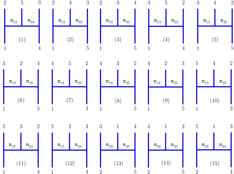
Figure 1: Independent structures of the color-dressed five-point scattering amplitudes of KK gauge bosons or KK gravitons at tree level, where the numbers $\{1,\cdots,5\}$ denote the KK indices of the external KK states, $\{1,\cdots,5\}\!\sim\{\mathfrak{n}_{1},\cdots,\mathfrak{n}_{5}\}$, and each internal line has its KK index $\mathfrak{n}_{ij}\!=\mathfrak{n}_{i}\!+\mathfrak{n}_{j}\hskip 0.85358pt$.

The above analyses of the four-point KK scattering amplitudes can be further extended to the $N$-point scattering amplitudes with $\hskip 0.85358ptN\!\geqslant 5\hskip 1.42262pt$. In this subsection, we study the double-copy construction of the five-point massive KK graviton scattering amplitudes with external states having KK indices $(\mathfrak{n}_{1},\mathfrak{n}_{2},\mathfrak{n}_{3},\mathfrak{n}_{4},\mathfrak{n}_{5})$.

There are 15 independent structures of the five-point scattering amplitudes of the KK gauge bosons or KK gravitons, and each structure contains two kinematic poles in total, which we present in Fig. 1. Thus, using the extended massive BCJ-type double-copy formula (24) of the $N$-point KK graviton amplitudes, we can derive the structure of the general five-point scattering amplitudes of KK gravitons under the $S^{1}$ compactification. For each given combination of KK indices $\{\mathfrak{n}_{1},\cdots\!,\mathfrak{n}_{5}\}$ of external states, we can construct the KK graviton scattering amplitude as follows:

$$\mathcal{M}\big{[}h_{\mathfrak{n}_{1}}^{\sigma_{1}}h_{\mathfrak{n}_{2}}^{\sigma_{2}}h_{\mathfrak{n}_{3}}^{\sigma_{3}}h_{\mathfrak{n}_{4}}^{\sigma_{4}}h_{\mathfrak{n}_{5}}^{\sigma_{5}}\big{]}=\frac{~{}\kappa^{3}\,}{64}\!\sum_{\lambda_{k},\lambda^{\prime}_{k}}\!\prod_{k=1}^{5}\!C_{\lambda_{k}\lambda^{\prime}_{k}}^{\hskip 0.85358pt\sigma_{k}}\Bigg{[}\frac{\mathcal{N}_{1}\mathcal{N}^{\prime}_{1}}{(s_{12}\!-\!M_{12}^{2})(s_{34}\!-\!M_{34}^{2})}+\frac{\mathcal{N}_{2}\mathcal{N}^{\prime}_{2}}{(s_{12}\!-\!M_{12}^{2})(s_{35}\!-\!M_{35}^{2})}\hskip 17.07164pt$$

$$\qquad\hskip 22.76219pt+\frac{\mathcal{N}_{3}\mathcal{N}^{\prime}_{3}}{(s_{12}\!-\!M_{12}^{2})(s_{45}\!-\!M_{45}^{2})}+\frac{\mathcal{N}_{4}\mathcal{N}^{\prime}_{4}}{(s_{13}\!-\!M_{13}^{2})(s_{24}-M_{24}^{2})}+\frac{\mathcal{N}_{5}\mathcal{N}^{\prime}_{5}}{(s_{13}\!-\!M_{13}^{2})(s_{25}-M_{25}^{2})}$$

$$\qquad\hskip 22.76219pt+\frac{\mathcal{N}_{6}\mathcal{N}^{\prime}_{6}}{(s_{13}\!-\!M_{13}^{2})(s_{45}\!-\!M_{45}^{2})}+\frac{\mathcal{N}_{7}\mathcal{N}^{\prime}_{7}}{(s_{14}\!-\!M_{14}^{2})(s_{23}-M_{23}^{2})}+\frac{\mathcal{N}_{8}\mathcal{N}^{\prime}_{8}}{(s_{14}\!-\!M_{14}^{2})(s_{25}-M_{25}^{2})}$$

$$\qquad\hskip 22.76219pt+\frac{\mathcal{N}_{9}\mathcal{N}^{\prime}_{9}}{(s_{14}\!-\!M_{14}^{2})(s_{35}\!-\!M_{35}^{2})}+\frac{\mathcal{N}_{10}\mathcal{N}^{\prime}_{10}}{(s_{15}\!-\!M_{15}^{2})(s_{23}-M_{23}^{2})}+\frac{\mathcal{N}_{11}\mathcal{N}^{\prime}_{11}}{(s_{15}\!-\!M_{15}^{2})(s_{24}-M_{24}^{2})}$$

$$\qquad\hskip 22.76219pt+\frac{\mathcal{N}_{12}\mathcal{N}^{\prime}_{12}}{(s_{15}\!-\!M_{15}^{2})(s_{34}\!-\!M_{34}^{2})}+\frac{\mathcal{N}_{13}\mathcal{N}^{\prime}_{13}}{(s_{23}-M_{23}^{2})(s_{45}\!-\!M_{45}^{2})}+\frac{\mathcal{N}_{14}\mathcal{N}^{\prime}_{14}}{(s_{24}-M_{24}^{2})(s_{35}\!-\!M_{35}^{2})}$$

$$\qquad\hskip 22.76219pt+\frac{\mathcal{N}_{15}\mathcal{N}^{\prime}_{15}}{(s_{25}-M_{25}^{2})(s_{34}\!-\!M_{34}^{2})}\Bigg{]}.$$ (96)

In the above amplitude, for simplicity we have used the shorthand notations of the shifted massive numerators which are given by

$$\{\mathcal{N}_{j},\,\mathcal{N}_{j}^{\prime}\}\hskip 0.85358pt=\hskip 0.85358pt\{\mathcal{N}_{j}(\lambda_{k}),\,\mathcal{N}_{j}(\lambda^{\prime}_{k})\}\Big{|}_{s_{j}\rightarrow\hskip 1.42262pts_{j}-\hskip 0.85358ptM_{\mathfrak{n}\mathfrak{n}_{j}}^{2}},$$ (97)

where we also make the replacements for products of the external-state polarizations and momenta $\hat{\zeta}_{i}\!\cdot\hat{p}_{j}\!=\zeta_{i}\cdot p_{j}$ and $\hat{\zeta}_{i}\cdot\hat{\zeta}_{j}=\zeta_{i}\cdot\zeta_{j}\,$ according to Eq.(12). On the right-hand side of Eq.(97), the kinematic numerators $\{\mathcal{N}_{j}(\lambda_{k}),\,\mathcal{N}_{j}(\lambda^{\prime}_{k})\}$ are given by the corresponding five-point massless gauge boson amplitudes. The kinematic numerators of the five-point massless gauge boson amplitudes were studied in many literatures BCJ:2019 and can be obtained by a number of methods, such as the direct Feynman diagram calculation, the CHY formula, and the low energy limit of open string amplitudes.  To save space we will not list all the explicit formulas of these five-point massless numerators. As an example, we consider a sample five-point scattering amplitude of the inelastic process $(2n,n)\!\rightarrow\!(n,n,n)$, where all the external KK states are chosen to be $\mathbb{Z}_{2}$ even. Thus, given the condition of the KK number conservation $\sum_{i=1}^{5}\mathfrak{n}_{i}\!=\!0\hskip 0.85358pt$ for each KK sub-amplitude, we find the following allowed sub-amplitudes with their external KK gauge bosons (gravitons) having the KK-numbers:

$$\{+2n,+n,-n,-n,-n\}\hskip 0.85358pt,\hskip 7.11317pt\{+2n,-n,+n,-n,-n\}\hskip 0.85358pt,\hskip 7.11317pt\{+2n,-n,-n,+n,-n\}\hskip 0.85358pt,$$

$$\{+2n,-n,-n,-n,+n\}\hskip 0.85358pt,\hskip 7.11317pt\{\mathrm{all\ permutations\ of\ \left(+,-\right)}\},$$ (98)

where for convenience we assign the external state-1 to have the KK number $+2n\hskip 0.85358pt$.  For instance, we can explicitly construct the KK longitudinal graviton scattering amplitude with the external KK-number combination $\{+2n,+n,-n,-n,-n\}$:

$$\mathcal{M}\big{[}h^{+2n}_{L}h^{+n}_{L}h^{-n}_{L}h^{-n}_{L}h^{-n}_{L}\big{]}\hskip 0.85358pt=\hskip 0.85358pt\frac{~{}\kappa^{3}\,}{64}\!\sum_{\lambda_{k},\lambda^{\prime}_{k}}\!\prod_{k=1}^{5}\!C_{\lambda_{k}\lambda^{\prime}_{k}}^{\hskip 0.85358pt0}\Bigg{[}\frac{\mathcal{N}_{1}\mathcal{N}^{\prime}_{1}}{\,(s_{12}\!-\!9M_{n}^{2})(s_{34}\!-\!4M_{n}^{2})\,}$$

$$~{}+\frac{\mathcal{N}_{2}\mathcal{N}^{\prime}_{2}}{(s_{12}\!-\!9M_{n}^{2})(s_{35}\!-\!4M_{n}^{2})}+\frac{\mathcal{N}_{3}\mathcal{N}^{\prime}_{3}}{(s_{12}\!-\!9M_{n}^{2})(s_{45}\!-\!4M_{n}^{2})}+\frac{\mathcal{N}_{4}\mathcal{N}^{\prime}_{4}}{(s_{13}\!-\!M_{n}^{2})s_{24}}+\frac{\mathcal{N}_{5}\mathcal{N}^{\prime}_{5}}{(s_{13}\!-\!M_{n}^{2})s_{25}}$$

$$~{}+\frac{\mathcal{N}_{6}\mathcal{N}^{\prime}_{6}}{(s_{13}\!-\!M_{n}^{2})(s_{45}\!-\!4M_{n}^{2})}+\frac{\mathcal{N}_{7}\mathcal{N}^{\prime}_{7}}{(s_{14}\!-\!M_{n}^{2})s_{23}}+\frac{\mathcal{N}_{8}\mathcal{N}^{\prime}_{8}}{(s_{14}\!-\!M_{n}^{2})s_{25}}+\frac{\mathcal{N}_{9}\mathcal{N}^{\prime}_{9}}{(s_{14}\!-\!M_{n}^{2})(s_{35}\!-\!4M_{n}^{2})}$$

$$~{}+\frac{\mathcal{N}_{10}\mathcal{N}^{\prime}_{10}}{(s_{15}\!-\!M_{n}^{2})s_{23}}+\frac{\mathcal{N}_{11}\mathcal{N}^{\prime}_{11}}{(s_{15}\!-\!M_{n}^{2})s_{24}}+\frac{\mathcal{N}_{12}\mathcal{N}^{\prime}_{12}}{(s_{15}\!-\!M_{n}^{2})(s_{34}\!-\!4M_{n}^{2})}+\frac{\mathcal{N}_{13}\mathcal{N}^{\prime}_{13}}{s_{23}(s_{45}\!-\!4M_{n}^{2})}$$

$$~{}+\frac{\mathcal{N}_{14}\mathcal{N}^{\prime}_{14}}{s_{24}(s_{35}\!-\!4M_{n}^{2})}+\frac{\mathcal{N}_{15}\mathcal{N}^{\prime}_{15}}{s_{25}(s_{34}\!-\!4M_{n}^{2})}\Bigg{]}\,.$$ (99)

The five-point KK graviton scattering amplitudes with other combinations of the external KK indices given in Eq.(3.4) can be constructed in the similar manner.

3.5 Nonrelativistic Scattering Amplitudes of KK States

The KK compactification predicts an infinite tower of KK states for each type of particles in the compactified 4d effective theory, which serve as the KK excitation states of the corresponding zero-mode state. The KK mass spectrum always contains many heavy KK states, so they can have KK masses much larger than their kinetic energy and thus become nonrelativistic. Hence it is interesting to study how such nonrelativistic scattering amplitudes of heavy KK states behave. In addition, there are recent studies to extract the classical observables in the weak gravitational systems by calculating scattering amplitude BernC1 CalAmp-Rev . In these toy models, the macroscopic star or black holes are treated as super massive particles.  Their classical gravitational potential is be obtained by computing the four-point scattering amplitudes, while the testable gravitational wave signals can be calculated in term of the five-point scattering amplitudes. This motivates us to study the scattering amplitudes of the super massive KK states through the gravitational interactions and examine their behavior in the nonrelativistic limit. 

3.5.1. Nonrelativistic Scattering Amplitudes of KK Gauge Bosons/Gravitons

We consider the four-point KK graviton amplitudes in the nonrelativistic limit under low energy expansion $M_{n}^{2}\!\gg\!q^{2}\hskip 0.85358pt$, where $\hskip 0.85358ptq\hskip 0.85358pt$ denotes the magnitude of the 3-momentum of the initial or final states of KK particles. For the inelastic channel $\{0,0,n,n\}$, we have the magnitude of the 3-momentum of the massless initial state $\hskip 0.85358ptq\!=\!E_{n}\hskip 0.85358pt$ and the magnitude of the 3-momentum of the KK final state $\hskip 0.85358ptq^{\prime}\!=\!\sqrt{E_{n}^{2}\!-\!M_{n}^{2}\,}\!\ll\!M_{n}^{2}\hskip 0.85358pt$. Thus, with the full KK gauge boson scattering amplitude in Eq.(55) and Eq.(204) (Appendix B), we derive the following expanded nonrelativistic results at the LO and NLO:

$$\mathcal{T}_{0}[A_{\pm 1}^{a0}A_{\mp 1}^{b0}A_{L}^{cn}A_{L}^{dn}] =\hskip 0.85358ptg^{2}(\mathcal{C}_{u}-\mathcal{C}_{t})(1-c_{\theta})\hskip 0.85358pt,$$ (100a)

$$\delta\mathcal{T}[A_{\pm 1}^{a0}A_{\mp 1}^{b0}A_{L}^{cn}A_{L}^{dn}] =-\frac{\,g^{2}\hskip 0.85358ptq^{\prime}\,}{~{}2M_{n}\,}\hskip 0.85358pt\mathcal{C}_{s}\hskip 0.85358pt(c_{\theta}-c_{3\theta})\hskip 0.85358pt,$$ (100b)

where we have applied the 5d orbifold compactification of $S^{1}\!/\mathbb{Z}_{2}$. Then, using the full KK graviton scattering amplitude (219) of Appendix C, we derive the following expanded nonrelativistic results at the LO and NLO:

$$\mathcal{M}_{0}\big{[}h^{0}_{\pm 2}h^{0}_{\mp 2}h^{n}_{L}h^{n}_{L}\big{]} =\mathcal{M}_{0}\big{[}h^{0}_{\pm 2}h^{0}_{\mp 2}h^{\pm n}_{L}h^{\mp n}_{L}\big{]}=\frac{~{}3\hskip 0.85358pt\kappa^{2}M_{n}^{2}\,}{32}(3-4\hskip 0.85358ptc_{2\theta}\!+c_{4\theta})\hskip 0.85358pt,$$ (101a)

$$\delta\mathcal{M}\big{[}h^{0}_{\pm 2}h^{0}_{\mp 2}h^{n}_{L}h^{n}_{L}\big{]} =\delta\mathcal{M}\big{[}h^{0}_{\pm 2}h^{0}_{\mp 2}h^{\pm n}_{L}h^{\mp n}_{L}\big{]}=\frac{~{}3\hskip 0.85358pt\kappa^{2}q^{\prime\hskip 0.85358pt2}\,}{128}(2-c_{2\theta}\!-2\hskip 0.85358ptc_{4\theta}\!+c_{6\theta})\hskip 0.85358pt.$$ (101b)

We see that for the inelastic channel of $\{0,0,n,n\}$, the LO KK amplitude is of $O(M_{n}^{2}q^{0})$ and the NLO KK amplitude has $O(M_{n}^{0}q^{2})\hskip 0.85358pt$.

Next, we consider the nonrelativistic limit of the elastic KK gauge boson/graviton scattering channel $\{n,n,n,n\}$. With the full KK gauge boson scattering amplitude in Eq.(71) and Eqs. (213)-(217) (Appendix B), we derive the following expanded nonrelativistic results at the LO and NLO:

$$\mathcal{T}_{\hskip 0.85358pt0}[A_{L}^{an}A_{L}^{bn}A_{L}^{cn}A_{L}^{dn}] =\frac{~{}g^{2}M_{n}^{2}~{}}{q^{2}}\!\left[\mathcal{C}_{t}\frac{~{}1+c_{2\theta}~{}}{1+c_{\theta}}+\mathcal{C}_{u}\frac{\,-(1+c_{2\theta})~{}}{1-c_{\theta}}\right]\!,$$ (102a)

$$\delta\mathcal{T}[A_{L}^{an}A_{L}^{bn}A_{L}^{cn}A_{L}^{dn}] =g^{2}\!\left[\mathcal{C}_{s}\frac{\hskip 0.85358pt-9\hskip 0.85358ptc_{\theta}\,}{2}+\mathcal{C}_{t}\frac{\,4\!-\!19\hskip 0.85358ptc_{\theta}\!-6\hskip 0.85358ptc_{2\theta}\!+c_{3\theta}}{4\hskip 0.85358pt(1+c_{\theta})}+\mathcal{C}_{u}\frac{\,-(4\!+\!19\hskip 0.85358ptc_{\theta}\!-6\hskip 0.85358ptc_{2\theta}\!-c_{3\theta})\,}{4\hskip 0.85358pt(1-c_{\theta})}\right]\!.$$ (102b)

We note that the LO elastic KK gauge boson amplitude $\mathcal{T}_{0}$ has $O(M_{n}^{2}\hskip 0.85358ptq^{-2})$ and exhibits a low energy behavior of $\,1/q^{2}\,$ due to the exchange of massless zero modes in the $t$ and $u$ channels with the momentum transfer $Q^{2}\!=2q^{2}(1\!\pm c_{\theta})$, where $Q^{2}\!=\!-t$ or $Q^{2}\!=\!-u\hskip 0.85358pt$. It is worth to note that after Fourier transformation, this $\,1/Q^{2}\,$ behavior reproduces the classical Coulomb potential $1/\hskip 0.85358ptr\,$.

Then, using the double-copied full KK graviton amplitudes (230)-(234) of Appendix C, we derive the following expanded nonrelativistic partial amplitudes at the LO:

$${\mathcal{M}}_{0}\big{[}h_{L}^{\pm n}h_{L}^{\pm n}h_{L}^{\mp n}h_{L}^{\mp n}\big{]} =0\,,$$ (103a)

$${\mathcal{M}}_{0}\big{[}h_{L}^{\pm n}h_{L}^{\mp n}h_{L}^{\mp n}h_{L}^{\pm n}\big{]} =\frac{~{}\kappa^{2}M_{n}^{4}\hskip 0.85358pt(11+12\hskip 0.85358ptc_{\theta}+9\hskip 0.85358ptc_{2\theta})~{}}{16\hskip 0.85358pt(1-c_{\theta})\hskip 0.85358ptq^{2}}\,,$$ (103b)

$${\mathcal{M}}_{0}\big{[}h_{L}^{\pm n}h_{L}^{\mp n}h_{L}^{\pm n}h_{L}^{\mp n}\big{]} =\frac{~{}\kappa^{2}M_{n}^{4}\hskip 0.85358pt(11+12c_{\theta}+9c_{2\theta})~{}}{16\hskip 0.85358pt(1+c_{\theta})\hskip 0.85358ptq^{2}}\,.$$ (103c)

Under the 5d orbifold compactification of $S^{1}\!/\mathbb{Z}_{2}$, we further deduce the following LO amplitude with the external KK states being $\mathbb{Z}_{2}$ even:

$${\mathcal{M}}_{0}\big{[}h_{L}^{n}h_{L}^{n}h_{L}^{n}h_{L}^{n}\big{]}\! =\mbox{$\frac{\,{1}\,}{\,2\,}$}\!\left(\!\mathcal{M}_{0}\big{[}h_{L}^{\pm n}h_{L}^{\pm n}h_{L}^{\mp n}h_{L}^{\mp n}\big{]}\!+\!{\mathcal{M}}_{0}\big{[}h_{L}^{\pm n}h_{L}^{\mp n}h_{L}^{\mp n}h_{L}^{\pm n}\big{]}\!+\!{\mathcal{M}}_{0}\big{[}h_{L}^{\pm n}h_{L}^{\mp n}h_{L}^{\pm n}h_{L}^{\mp n}\big{]}\!\right)$$

$$=\frac{~{}\kappa^{2}M_{n}^{4}~{}}{8\hskip 1.42262ptq^{2}}(1\!+3\hskip 0.85358ptc_{2\theta})^{2}\csc^{2}\!\theta\hskip 0.85358pt.$$ (104)

We see that these LO elastic KK amplitudes have $O(M_{n}^{4}\hskip 0.85358ptq^{-2})$ and they exhibit a low energy behavior of $\,1/q^{2}\,$. This is due to the exchange of massless zero modes in the $t$ and/or $u$ channels with the momentum transfer $Q^{2}\!=2q^{2}(1\!\pm c_{\theta})$, where $Q^{2}\!=\!-t$ or $Q^{2}\!=\!-u\hskip 0.85358pt$. It is worth to note that after Fourier transformation, this $\,1/Q^{2}\,$ behavior reproduces the classical Newtonian gravitational potential $1/\hskip 0.85358ptr\,$.

Then, under the nonrelativistic expansion, we derive the following NLO KK amplitude for the elastic scattering channel $\{n,n,n,n\}$:

$$\delta\mathcal{M}\big{[}h_{L}^{\pm n}h_{L}^{\pm n}h_{L}^{\mp n}h_{L}^{\mp n}\big{]} =0\,,$$ (105a)

$$\delta\mathcal{M}\big{[}h_{L}^{\pm n}h_{L}^{\mp n}h_{L}^{\mp n}h_{L}^{\pm n}\big{]} =\frac{\kappa^{2}M_{n}^{2}}{\,64\hskip 0.85358pt(1\!-c_{\theta})\,}(102+22\hskip 0.85358ptc_{\theta}+72\hskip 0.85358ptc_{2\theta}+51\hskip 0.85358ptc_{3\theta}+18\hskip 0.85358ptc_{4\theta}-9\hskip 0.85358ptc_{5\theta})\hskip 0.85358pt,$$ (105b)

$$\delta\mathcal{M}\big{[}h_{L}^{\pm n}h_{L}^{\mp n}h_{L}^{\pm n}h_{L}^{\mp n}\big{]} =\frac{\kappa^{2}M_{n}^{2}}{\,64\hskip 0.85358pt(1\!+c_{\theta})\,}(102-22\hskip 0.85358ptc_{\theta}+72\hskip 0.85358ptc_{2\theta}-51\hskip 0.85358ptc_{3\theta}+18\hskip 0.85358ptc_{4\theta}+9\hskip 0.85358ptc_{5\theta})\hskip 0.85358pt,$$ (105c)

which are of $O(M_{n}^{2}q^{0})$ and energy-independent. For the 5d orbifold compactification of $S^{1}\!/\mathbb{Z}_{2}$, we further derive the corresponding NLO elastic KK amplitude:

$$\delta\mathcal{M}\big{[}h_{L}^{n}h_{L}^{n}h_{L}^{n}h_{L}^{n}\big{]}=\frac{~{}\kappa^{2}M_{n}^{2}~{}}{128}\hskip 0.85358pt(226+217\hskip 0.85358ptc_{\theta}+78\hskip 0.85358ptc_{4\theta}-9\hskip 0.85358ptc_{6\theta})\csc^{2}\!\theta\,,$$ (106)

which also has the magnitude of $O(M_{n}^{2}\hskip 0.85358ptq^{0})$.

3.5.2. Nonrelativistic KK Scattering Amplitudes with KK Graviton Exchange

For comparison with the above nonrelativistic pure KK gauge/gravity amplitudes, we consider the Einstein gravity coupled to scalar fields or gauge fields under the 5d KK compactification of $S^{1}\!/\mathbb{Z}_{2}$ and analyze the nonrelativistic scattering amplitudes of KK scalars (KK gauge bosons) through the KK graviton exchanges.

We first consider the 5d Einstein-Scalar (ES) theory as a toy model, which contains a massless real scalar field $\widehat{\Phi}$ coupled to gravity:

$$S_{\mathrm{ES}}\,=\,\int\!\!\mathrm{d}^{4}{x}\hskip 0.85358pt\mathrm{d}y\,\sqrt{\!-\hat{g}\,}\!\left(\!\frac{2}{~{}\hat{\kappa}^{2}\,}\widehat{R}+\frac{1}{\,2\,}\hat{g}_{\mu\nu}\partial^{\mu}\widehat{\Phi}\hskip 0.85358pt\partial^{\nu}\widehat{\Phi}\right)\!,$$ (107)

Under the 5d compactification, we make the KK expansion of $\widehat{\Phi}$ and derive the trilinear KK scalar-graviton interaction vertex $\hskip 0.85358pt\phi_{n}$$-$$\phi_{m}$$-$$h_{k}^{\mu\nu}$ and the KK scalar-radion interaction vertex $\hskip 0.85358pt\phi_{n}$$-$$\phi_{m}$$-$$h_{0}^{55}$. Thus, we can compute the four-point scalar scattering amplitudes with zero-mode and KK graviton-exchanges as well as the radion exchange. For the inelastic channel $\phi_{0}\hskip 0.85358pt\phi_{0}\!\rightarrow\!\phi_{n}\hskip 0.85358pt\phi_{n}$, we derive the following scattering amplitude:

$$\mathcal{T}_{\hskip 0.85358pth}[\phi_{0}\phi_{0}\phi_{n}\phi_{n}]\,=\,-\frac{~{}\kappa^{2}M_{n}^{2}\hskip 0.85358pt\big{[}(7\hskip 0.85358pt\bar{s}+4)+(\bar{s}+4)\hskip 0.85358ptc_{2\theta}\hskip 0.85358pt\big{]}^{2}~{}}{32\hskip 0.85358pt\big{[}(\bar{s}+4)-(\bar{s}-4)\hskip 0.85358ptc_{2\theta}\big{]}}\,,$$ (108)

where $\hskip 0.85358pt\bar{s}=s/M_{n}^{2}\!=4\hskip 0.85358pt(\bar{q}^{\hskip 0.85358pt\prime\hskip 0.85358pt2}\!+1)\hskip 0.85358pt$ and $\bar{q}^{\hskip 0.85358pt\prime}\!={q}^{\hskip 0.85358pt\prime}/M_{n}\hskip 0.85358pt$. We have verified the above amplitude by using the shifting method of Sec. 2.2 to derive the massive KK amplitude from computing the corresponding 5d massless amplitude. Then, from Eq.(108) we make the nonrelativistic expansion $\hskip 0.85358ptq^{\prime\hskip 0.85358pt2}\!\ll\!M_{n}^{2}\hskip 0.85358pt$, and derive the following LO and NLO scalar amplitudes:

$$\mathcal{T}_{\hskip 0.85358pth}^{(0)}[\phi_{0}\phi_{0}\phi_{n}\phi_{n}] \hskip 0.85358pt=\hskip 0.85358pt-\frac{\,9\,}{\,4\,}{\kappa^{2}M_{n}^{2}}\,,$$ (109a)

$$\delta\mathcal{T}_{\hskip 0.85358pth}[\phi_{0}\phi_{0}\phi_{n}\phi_{n}] \hskip 0.85358pt=\hskip 0.85358pt-\frac{\,3\,}{\,8\,}{\kappa^{2}q^{\hskip 0.85358pt\prime\hskip 0.85358pt2}}(11\!+5\hskip 0.85358ptc_{2\theta})\hskip 0.85358pt.$$ (109b)

We see that the LO and NLO amplitudes are of $O(\kappa^{2}M_{n}^{2})$ and $O(\kappa^{2}q^{\hskip 0.85358pt\prime\hskip 0.85358pt2})$, respectively.

For the elastic channel $\{n,n,n,n\}$, we compute the KK scalar scattering amplitude as follows:

$$\mathcal{T}_{\hskip 0.85358pth}[\phi_{n}\phi_{n}\phi_{n}\phi_{n}]=-\frac{~{}\kappa^{2}M_{n}^{2}\hskip 0.85358pt(X_{0}\!+\!X_{2}\hskip 0.85358ptc_{2\theta}\!+\!X_{4}c_{4\theta}\!+\!X_{6}\hskip 0.85358ptc_{6\theta})\csc^{2}\!\theta~{}}{~{}512\hskip 0.85358pt\bar{s}\hskip 0.85358pt(\bar{s}-4)\big{[}(\bar{s}^{2}+24\hskip 0.85358pt\bar{s}+16)-(\bar{s}-4)^{2}c_{2\theta}\big{]}~{}}\,,$$ (110)

where $\hskip 0.85358pt\bar{s}=s/M_{n}^{2}\!=4\hskip 0.85358pt(\bar{q}^{2}\!+\!1)\hskip 0.85358pt$ with $\bar{q}={q}/M_{n}\hskip 0.85358pt$, and the polynomial functions $\{X_{j}\}$ take the following form:

$$X_{0} =510\hskip 0.85358pt\bar{s}^{5}\!+8144\hskip 0.85358pt\bar{s}^{4}\!-27584\hskip 0.85358pt\bar{s}^{3}\!+61440\hskip 0.85358pt\bar{s}^{2}\!+60928\hskip 0.85358pt\bar{s}+28672\hskip 0.85358pt,$$

$$X_{2} =-429\hskip 0.85358pt\bar{s}^{5}\!+6984\hskip 0.85358pt\bar{s}^{4}\!-30816\hskip 0.85358pt\bar{s}^{3}\!+51712\hskip 0.85358pt\bar{s}^{2}\!-42240\hskip 0.85358pt\bar{s}-34816\hskip 0.85358pt,$$

$$X_{4} =-78\hskip 0.85358pt\bar{s}^{5}\!+1200\hskip 0.85358pt\bar{s}^{4}\!-6720\hskip 0.85358pt\bar{s}^{3}\!+16384\hskip 0.85358pt\bar{s}^{2}\!-\!15872\hskip 0.85358pt\bar{s}+4096\hskip 0.85358pt,$$

$$X_{6} =-3\hskip 0.85358pt\bar{s}^{5}\!+56\hskip 0.85358pt\bar{s}^{4}\!-416\hskip 0.85358pt\bar{s}^{3}\!+1536\hskip 0.85358pt\bar{s}^{2}\!-2816\hskip 0.85358pt\bar{s}+2048\,.$$

Thus, making the nonrelativistic expansion $\hskip 0.85358ptq^{2}\!\ll\!M_{n}^{2}\hskip 0.85358pt$, we derive the following KK scalar scattering amplitudes at the LO and NLO:

$$\mathcal{T}_{\hskip 0.85358pth}^{(0)}[\phi_{n}\phi_{n}\phi_{n}\phi_{n}] =\hskip 0.85358pt-\frac{~{}2\hskip 0.85358pt\kappa^{2}M_{n}^{4}\csc^{2}\!\theta~{}}{q^{2}}\hskip 0.85358pt,$$ (112a)

$$\delta\mathcal{T}_{\hskip 0.85358pth}[\phi_{n}\phi_{n}\phi_{n}\phi_{n}] =\hskip 0.85358pt-\frac{1}{\,2\,}\kappa^{2}M_{n}^{2}\hskip 0.85358pt{(7+c_{2\theta})}\csc^{2}\!\theta\hskip 0.85358pt,$$ (112b)

whose magnitudes are of $O(\kappa^{2}M_{n}^{4}/q^{2})$ and $O(\kappa^{2}M_{n}^{2})$, respectively. Note that the LO elastic KK scalar amplitude (112a) also exhibits a low energy behavior of $\,1/q^{2}\,$ due to the exchange of massless zero modes in the $t$ and $u$ channels with the momentum transfer $Q^{2}\!=2q^{2}(1\!\pm c_{\theta})$, where $Q^{2}\!=\!-t$ or $Q^{2}\!=\!-u\hskip 0.85358pt$. This is similar to the LO amplitudes of the pure KK gauge boson (KK graviton) scattering in Eqs.(102a) and (3.5). After a Fourier transformation such $\,1/Q^{2}\,$ behavior recovers the classical Newtonian gravitational potential of $1/r$ at low energy. We also see that the NLO KK amplitude (112b) behaves as $q$-independent constant term.

Next, for comparison we further consider the 5d gauge theory coupled to GR, which has the following 5d action:

$$S_{\mathrm{GRA}}\,=\,\int\!\!\mathrm{d}^{4}{x}\hskip 0.85358pt\mathrm{d}y\,\sqrt{\!-\hat{g}\,}\left(\!\frac{2}{~{}\hat{\kappa}^{2}\,}\widehat{R}-\frac{1}{\,4\,}\hat{g}^{\mu\alpha}\hat{g}^{\nu\beta}\widehat{F}^{\hskip 0.85358pta}_{\mu\nu}\widehat{F}^{\hskip 0.85358pta}_{\alpha\beta}\right)\!,$$ (113)

where $\widehat{F}^{\hskip 0.85358pta}_{\mu\nu}$ is the 5d gauge field strength of a non-Abelian gauge group of YM theory or Abelian gauge group of Maxwell theory (with $a\!=\!1$). Under the 5d compactification, we derive the 4d KK theory which includes the trilinear KK gauge-boson-graviton interaction vertex $\hskip 0.85358ptA_{n}^{a\hskip 0.85358pt\mu}$$-$$A_{m}^{b\hskip 0.85358pt\nu}$$-$$h_{k}^{\mu\nu}$. Then, we will compute the four-point KK gauge boson scattering amplitudes with graviton exchange and derive the nonrelativistic results at low energy, which should be compared to the nonrelativistic KK scalar amplitudes we derived for the Einstein-Scalar theory (107). For the case of non-Abelian gauge theory, the four-point KK gauge boson amplitudes will also receive the contribution by pure gauge interactions including the contact gauge vertex and the gauge boson exchange via cubic gauge vertex. But such pure gauge contribution is gauge-invariant by itself and has already been computed in Sec. 3.5.1 and Sec. 3.2-3.3. So, in the following we will focus on analyzing the nonrelativistic KK gauge boson amplitudes through the graviton exchanges and compare them with the nonrelativistic KK scalar amplitudes which we derived in the first part of Sec. 3.5.2.

For the inelastic channel $\{0,0,n,n\}$, we compute the four-point gauge boson scattering amplitude via graviton and radion exchanges:

$$\mathcal{T}_{\hskip 0.85358pth}\big{[}A_{\pm 1}^{a0}A_{\pm 1}^{a0}A_{L}^{bn}\!A_{L}^{bn}\big{]}\hskip 0.85358pt=\hskip 0.85358pt\frac{~{}\kappa^{2}M_{n}^{2}\big{[}(3\hskip 0.85358pt\bar{s}^{2}\!+\!18\hskip 0.85358pt\bar{s}-8)-(3\hskip 0.85358pt\bar{s}^{2}\!-\!14\hskip 0.85358pt\bar{s}+8)\hskip 0.85358ptc_{2\theta}\hskip 0.85358pt\big{]}~{}}{8\hskip 0.85358pt\big{[}(\bar{s}+4)-(\bar{s}-4)\hskip 0.85358ptc_{2\theta}\hskip 0.85358pt\big{]}}\,.$$ (114)

Then, we make the nonrelativistic expansion and derive the LO and NLO scattering amplitudes as follows:

$$\mathcal{T}_{\hskip 0.85358pth}^{(0)}\big{[}A_{\pm 1}^{a0}A_{\pm 1}^{a0}A_{L}^{bn}\!A_{L}^{bn}\big{]} =\frac{7}{\,4\,}\hskip 0.85358pt\kappa^{2}M_{n}^{2}\,,$$ (115a)

$$\delta\mathcal{T}_{\hskip 0.85358pth}\big{[}A_{\pm 1}^{a0}A_{\pm 1}^{a0}A_{L}^{bn}\!A_{L}^{bn}\big{]} =\frac{1}{\,4\,}\kappa^{2}q^{\hskip 0.85358pt\prime\hskip 0.85358pt2}(7+c_{2\theta})\hskip 0.85358pt.$$ (115b)

The above LO and NLO amplitudes are of $O(\kappa^{2}M_{n}^{2})$ and $O(\kappa^{2}q^{\hskip 0.85358pt\prime\hskip 0.85358pt2})$ respectively. These have the same structures as that of the corresponding LO and NLO scalar amplitudes in Eq.(109), except that the angular dependence of the above NLO amplitude (115b) has different coefficients from that of Eq.(109b).

For the elastic channel $\{n,n,n,n\}$, we first consider all the external KK gauge bosons having transverse polarizations with the helicity indices $(\pm 1,\pm 1,\pm 1,\pm 1)$. Thus, we compute their elastic scattering amplitude as follows:

$$\mathcal{T}_{\hskip 0.85358pth}\big{[}A_{\pm 1}^{an}A_{\pm 1}^{an}A_{\pm 1}^{bn}A_{\pm 1}^{bn}\big{]}=-\frac{~{}\kappa^{2}M_{n}^{2}\big{[}(3\hskip 0.85358pt\bar{s}^{2}\!-\!11\hskip 0.85358pt\bar{s}+\!12)-(\bar{s}\!-\!4)c_{2\theta}\big{]}~{}}{2\hskip 0.85358pt\bar{s}\hskip 0.85358pt(\bar{s}-4)}\hskip 0.85358pt,$$ (116)

where $\hskip 0.85358pt\bar{s}=s/M_{n}^{2}\!=4\hskip 0.85358pt(\bar{q}^{2}\!+\!1)\hskip 0.85358pt$ with $\bar{q}={q}/M_{n}\hskip 0.85358pt$. Then, we make the nonrelativistic expansion and derive the following LO and NLO elastic scattering amplitudes:

$$\mathcal{T}_{\hskip 0.85358pth}^{(0)}\big{[}A_{\pm 1}^{an}A_{\pm 1}^{an}A_{\pm 1}^{bn}A_{\pm 1}^{bn}\big{]} =-\frac{~{}\kappa^{2}M_{n}^{4}~{}}{2\hskip 0.85358ptq^{2}}\,,$$ (117a)

$$\delta\mathcal{T}_{\hskip 0.85358pth}\big{[}A_{\pm 1}^{an}A_{\pm 1}^{an}A_{\pm 1}^{bn}A_{\pm 1}^{bn}\big{]} =-\frac{1}{\,8\,}\kappa^{2}M_{n}^{2}\hskip 0.85358pt(9-c_{2\theta})\hskip 0.85358pt.$$ (117b)

We see that the LO nonrelativistic KK amplitude (117a) exhibits a low energy behavior $\,1/q^{2}\,$ due to the exchange of massless zero modes in the $t$ and $u$ channels which is similar to the LO KK scalar amplitude (112a). But, the above LO and NLO KK gauge boson scattering amplitudes have different angular structures from that of the elastic KK scalar scattering amplitudes (112).

Finally, we compute the four-point elastic longitudinal KK gauge boson scattering amplitude via the graviton and radion exchanges:

$$\mathcal{T}_{\hskip 0.85358pth}\big{[}A_{L}^{an}\!A_{L}^{an}\!A_{L}^{bn}\!A_{L}^{bn}\big{]}=-\frac{~{}\kappa^{2}M_{n}^{2}\hskip 0.85358pt\big{(}X_{0}+X_{2}\hskip 0.85358ptc_{2\theta}+\!X_{4}\hskip 0.85358ptc_{4\theta}+\!X_{6}\hskip 0.85358ptc_{6\theta}\big{)}\csc^{2}\!\theta~{}}{~{}512\hskip 0.85358pt\bar{s}\hskip 0.85358pt(\bar{s}-4)\big{[}(\bar{s}^{2}\!+24\hskip 0.85358pt\bar{s}+\!16)-(\bar{s}-4)^{2}c_{2\theta}\big{]}~{}}\,,$$ (118)

where $\hskip 0.85358pt\bar{s}\!=\!s/M_{n}^{2}\!=4\hskip 0.85358pt(\bar{q}^{2}+1)\hskip 0.85358pt$ with $\bar{q}\!=\!{q}/M_{n}\hskip 0.85358pt$, and the polynomial functions $\{X_{j}\}$ are expressed as follows:

$$X_{0} =510\hskip 0.85358pt\bar{s}^{5}\!+7696\hskip 0.85358pt\bar{s}^{4}\!-35520\hskip 0.85358pt\bar{s}^{3}\!+39936\hskip 0.85358pt\bar{s}^{2}\!+40448\hskip 0.85358pt\bar{s}+28672\hskip 0.85358pt,$$

$$X_{2} =-429\hskip 0.85358pt\bar{s}^{5}\!+7528\hskip 0.85358pt\bar{s}^{4}\!-25056\hskip 0.85358pt\bar{s}^{3}\!+77824\hskip 0.85358pt\bar{s}^{2}\!-\!11520\hskip 0.85358pt\bar{s}-34816\hskip 0.85358pt,$$

$$X_{4} =-78\hskip 0.85358pt\bar{s}^{5}\!+\!1136\hskip 0.85358pt\bar{s}^{4}\!-4928\hskip 0.85358pt\bar{s}^{3}\!+\!13312\hskip 0.85358pt\bar{s}^{2}\!-28160\hskip 0.85358pt\bar{s}+4096\hskip 0.85358pt,$$

$$X_{6} =-3\hskip 0.85358pt\bar{s}^{5}\!+24\hskip 0.85358pt\bar{s}^{4}\!-32\hskip 0.85358pt\bar{s}^{3}\!-768\hskip 0.85358pt\bar{s}+2048\hskip 0.85358pt.$$ (119)

From the above, we make the nonrelativistic expansion and derive the LO and NLO longitudinal KK scattering amplitudes as follows:

$$\mathcal{T}_{\hskip 0.85358pth}^{(0)}\big{[}A_{L}^{an}A_{L}^{an}A_{L}^{bn}A_{L}^{bn}\big{]} =-\frac{~{}2\hskip 0.85358pt\kappa^{2}M_{n}^{4}\cot^{2}\!\theta~{}}{q^{2}}=-\frac{~{}\kappa^{2}M_{n}^{4}~{}}{q^{2}}(1\!+c_{2\theta})\csc^{2}\!\theta\hskip 0.85358pt,$$ (120a)

$$\delta\mathcal{T}_{\hskip 0.85358pth}\big{[}A_{L}^{an}A_{L}^{an}A_{L}^{bn}A_{L}^{bn}\big{]} =-\frac{~{}\kappa^{2}M_{n}^{2}~{}}{8}(23+8\hskip 0.85358ptc_{2\theta}+c_{4\theta})\csc^{2}\!\theta\hskip 0.85358pt.$$ (120b)

The above can be compared to the LO and NLO amplitudes (117) with all the external KK states being transversely polarized, and they have different angular structures. Moreover, comparing the above nonrelativistic LO and NLO longitudinal KK scattering amplitudes with the scalar KK scattering amplitudes (112), we find that their LO amplitudes have the magnitude of $O(\kappa^{2}M_{n}^{4}/q^{2})$ and their NLO amplitudes are of $O(\kappa^{2}M_{n}^{2})$, but they have rather different angular structures at the LO and NLO respectively. These nontrivial differences of angular structures between the nonrelativistic KK scalar scattering amplitudes (112) and the KK gauge boson scattering amplitudes (117) are due to the different spins of the external KK states in the two cases and their different cubic interaction vertices with the internal gravitons. Such differences remain even in the nonrelativistic KK scattering amplitudes.

4 Worldsheet Formulation of Massive KK Double-Copy

The conventional Cachazo-He-Yuan (CHY) formalism CHY can be used to analyze the scattering amplitudes of the massless scalar, gauge, and gravity theories in terms of the localized integrals in the moduli space $\mathfrak{M}_{0,N}$ of the $N$-punctured genus-zero Riemann sphere $\mathbb{CP}^{1}$. Its physical origin is based on the ambitwistor string theory Mason:2013sva ; Geyer:2014fka ; Adamo:2013tsa ; Casali:2015vta . In this section, we generalize the conventional massless CHY scattering equations to the case of the massive KK scattering amplitudes under the 5d toroidal compactification. We derive an extended massive KK scattering equation for the KK scattering amplitudes in Section 4.1 and construct the KK bi-adjoint scalar amplitudes in Section 4.2. Then, in Section 4.3 we use this massive CHY approach to further construct the scattering amplitudes of KK gauge bosons and of KK gravitons, and derive their relations to the extended BCJ-type mmasive KK amplitudes (given in Section 3) and to the extended KLT-type masive KK amplitudes (formulated in Ref. KKString ).

4.1 Extended CHY Formulation of Massive KK Scattering Amplitudes

Consider the $(4+\delta)$-dimensional spacetime with $\delta$ extra spatial dimensions under the toroidal compactification. For a momentum $\hat{p}_{a}$ living in the $(4+\delta)$-dimensions, we can decompose it in the following form:

$$\hat{p}_{a}^{M}=\left(p_{a}^{\mu},\hskip 0.85358pt\frac{{\mathfrak{n}_{1}}}{\,R_{1}}\bigg{|}_{a}\hskip 0.85358pt,\cdots,\frac{{\mathfrak{n}_{\delta}}}{\,R_{\delta}}\bigg{|}_{a}\right)\!,\quad~{}~{}a\in\{1,\cdots,N\}\hskip 0.85358pt,$$ (121)

where $\,p^{\mu}_{a}\,$ and $\,(\mathfrak{n}_{i}/R_{i})\big{|}_{a}\,$ are the momenta defined in $(3\!+\!1)$-dimensions and $\delta$-dimensions respectively. For the simplicity of demonstration, we set $\hskip 0.85358pt\delta\!\!=\!1\hskip 0.85358pt$ with the compactification radius $\hskip 0.85358ptR_{1}\!=\!R$ . Hence, similar to Dolan Naculich we can express the $\mathrm{SL}(2,\mathbb{C})$ invariant scattering equation in the $(4\!+\!1)$-dimensional spacetime as follows:

$$\widehat{E}_{a}\,=\,\sum_{\begin{subarray}{c}b=1\\ (b\neq a)\end{subarray}}^{N}\!\!\frac{~{}\hat{p}_{a}\!\cdot\hat{p}_{b}~{}}{z_{a}\!-z_{b}}\,=\,\sum_{\begin{subarray}{c}b=1\\ (b\neq a)\end{subarray}}^{N}\!\!\frac{~{}p_{a}\!\cdot p_{b}+\!M^{2}_{ab}~{}}{z_{a}\!-z_{b}}\,=\,0\,,$$ (122)

where the $N$ holomorphic variables $\{z_{a}\}$ parametrize the moduli space $\mathfrak{M}_{0,N}$ of the $N$-punctured Riemann sphere $\mathbb{CP}^{1}$, and summation runs over the $\,(N\!-3)!\,$ solutions for $z_{a}$. The mass parameter in Eq.(122) is given by

$$M_{ab}^{2}=M_{ba}^{2}=\frac{~{}\mathfrak{n}_{a}\mathfrak{n}_{b}~{}}{R^{2}}\,.$$ (123)

As analyzed in Section 2.1, we find that each massive KK amplitude can be decomposed into a sum of higher dimensional sub-amplitudes in which the components of momenta associated with the compactified dimension are discretized. Hence, under the toroidal compactification, we can generalize the conventional CHY formulation of the gauge boson amplitude and graviton amplitude to the following forms:

$$\mathcal{A}_{N}\big{[}\{p_{i},\hat{\zeta}_{i},I_{i}\}\big{]} \,=\,\sum_{q_{j}}\!\widehat{\mathcal{A}}_{N}\big{[}\{p_{i},\hat{\zeta}_{i},q_{i}\}\big{]}\prod_{j}\!\int_{\mathbb{N}}\text{d}y_{j}\hskip 0.85358pte^{\text{i}q_{j}y_{j}}\mathcal{O}_{I_{j}}(y_{j})\hskip 0.85358pt,$$ (124a)

$$\mathcal{M}_{N}\big{[}\{p_{i},\hat{\zeta}_{i},I_{i}\}\big{]} \,=\,\sum_{q_{j}}\!\widehat{\mathcal{M}}_{N}\big{[}\{p_{i},\hat{\zeta}_{i},q_{i}\}\big{]}\prod_{j}\!\int_{\mathbb{N}}\text{d}y_{j}\hskip 0.85358pte^{\text{i}q_{j}y_{j}}\mathcal{O}_{I_{j}}(y_{j})\hskip 0.85358pt.$$ (124b)

On the right-hand side of Eq.(124), the amplitude $\widehat{\mathcal{A}}_{N}\hskip 0.85358pt$ is defined as

$$\widehat{\mathcal{A}}_{N}\big{[}\{\hat{p},\hat{\zeta}\}\big{]}=\,\int\!\!\underbrace{\frac{\text{d}^{N}\!z}{\,\mathrm{Vol}\hskip 0.85358pt[\hskip 0.85358pt\mathrm{SL}(2,\mathbb{C})]\,}\sideset{}{{}^{\prime}}{\prod}_{a=1}^{N}\!\delta\big{(}\widehat{E}_{a}\big{)}}_{\text{d}\mu_{N}}\widehat{\mathcal{I}}_{N}(\{\hat{p},\hat{\zeta},z\})\,,$$ (125)

where $\text{d}\mu_{N}$ is the measure and $\widehat{\mathcal{I}}_{N}$ is a theory-dependent integrand. The above product operation $\prod^{\prime}$ is defined by

$$\sideset{}{{}^{\prime}}{\prod}_{a=1}^{N}\!\delta\big{(}\widehat{E}_{a}\big{)}\,\equiv\,(z_{i}\!-z_{j})(z_{j}\!-z_{k})(z_{k}\!-z_{i})\prod_{\begin{subarray}{c}a=1\\ (a\neq i,j,k)\end{subarray}}^{N}\delta\big{(}\widehat{E}_{a}\big{)}\hskip 0.85358pt,$$ (126)

which excludes the choice of the three fixed points $(z_{i},z_{j},z_{k})\!=\!(0,1,\infty)$ on the Riemann sphere and is permutation invariant CHY . The scattering amplitude (125) is invariant under $\mathrm{SL}(2,\mathbb{C})$ transformation acting on the coordinates $\{z_{a}\}$. Moreover, it is well established that the conventional KLT relations for the $(4\!+\!1)$-dimensional scattering amplitudes of the massless gauge bosons ($\widehat{\mathcal{A}}_{N}$) and of the massless gavitons ($\widehat{\mathcal{M}}_{N}$) can be given by the CHY formalism:

$$\widehat{\mathcal{M}}_{N}\hskip 0.85358pt=\!\sum_{\{\alpha,\beta\}}\!\!\widehat{\mathcal{A}}_{N}[\alpha]\hskip 1.42262pt\widehat{\mathcal{K}}\hskip 1.42262pt[\alpha|\beta]\widehat{\mathcal{A}}_{N}[\beta]\,,$$ (127)

where $\{\alpha,\beta\}\!\in\!S_{N-3}\hskip 0.85358pt$ denote the linearly independent color-orderings of the $N$-point gauge boson amplitudes, and $\widehat{\mathcal{K}}\hskip 1.42262pt[\alpha|\beta]$ is the KLT kernel. Thus, combining the $(4+\!1)$-dimensional massless KLT formula (127) with Eq.(124), we derive the extended massive KLT-type relation under the toroidal compactification, which expresses the KK graviton scattering amplitude ($\mathcal{M}_{N}$) as products of two color-ordered KK gauge boson amplitudes ($\mathcal{A}_{N}$) together with a kernel ($\hskip 0.85358pt\mathcal{K}\hskip 0.85358pt$) as follows:

$$\mathcal{M}_{N}\big{[}{\{p_{k},\zeta^{\mu\nu}_{\sigma_{k}}\}}\big{]}=\hskip 0.85358ptc_{0}\sum_{\mathsf{P}}\!\!\sum_{\{\alpha,\hskip 0.85358pt\beta\}}\!\sum_{\lambda_{k}\lambda_{k}^{\prime}}\!\!\Big{(}\!\prod_{k}\!C^{\,\sigma_{k}}_{\lambda_{k}\lambda_{k}^{\prime}}\Big{)}\mathcal{A}_{N}\big{[}\alpha,\hskip 0.85358pt\zeta^{\mu}_{\lambda_{k}}\!,\{\mathfrak{n}_{i}\}\big{]}\mathcal{K}\!\left([\alpha|\beta],\!\{\mathfrak{n}_{i}\}\right)\mathcal{A}_{N}\big{[}\beta,\hskip 0.85358pt\zeta^{\nu}_{\lambda_{k}^{\prime}}\!,\{\mathfrak{n}_{i}\}\big{]}\hskip 0.85358pt,$$ (128)

where $\hskip 0.85358ptc_{0}\!=\!(-)^{N+1}[\kappa/(4g)]^{N-2}$ is the conversion constant between the gauge and gravity couplings as given by Eq.(23). In the above, $\{\mathfrak{n}_{i}\}$ denote the KK indices of the external states and $\mathsf{P}$ labels every possible combination of the signs of these KK indices $\{\mathfrak{n}_{i}\}$ which obeying the $N$-point neutral condition $\sum_{i=1}^{N}\mathfrak{n}_{i}\!=\!0$ KKString . In Eq.(128), $k$ counts the external states of each amplitude and $C_{\lambda_{k}\lambda_{k}^{\prime}}^{\sigma_{k}}$ denotes the coefficients of the polarization tensor $\hskip 0.85358pt\zeta^{\mu\nu}_{\sigma_{k}}$ of the $k$-th external KK graviton as defined in Eqs.(21) and (39). Finally, we note that the above formulation can be readily extended to the case of having two or more compactified extra dimensions.

In summary, our above analysis has extended the conventional massless CHY formulation of the KLT double-copy relations to the compactified massive KK gauge/gravity theories. In this massive KK CHY construction, the KLT kernel $\mathcal{K}\!\left([\alpha|\beta],\!\{\mathfrak{n}\}\right)$ is formulated as the inverse of amplitudes of the KK bi-ajoint scalar theory under the toroidal compactification and will be discussed in Section 4.3.

4.2 CHY Construction for Massive KK Bi-ajoint Scalar Amplitudes

Consider a massless bi-adjoint scalar (BAS) theory respecting the (global) color symmetry $\mathrm{U}(N)\!\otimes\!\mathrm{U}({N})\hskip 0.85358pt$. The simplest Lagrangian of such a BAS theory contains a cubic interaction term CHY . We can write down its Lagrangian formulation in 5d as follows:

$$\mathcal{L}_{\mathrm{BAS}}\,=\,\frac{1}{2}(\partial_{M}\widehat{\Phi}^{aa^{\prime}})^{2}+\frac{\hat{\lambda}}{\,3!\,}f^{abc}f^{a^{\prime}b^{\prime}c^{\prime}}\widehat{\Phi}^{aa^{\prime}}\widehat{\Phi}^{bb^{\prime}}\widehat{\Phi}^{cc^{\prime}}\!,$$ (129)

where $\hskip 0.85358pt\hat{\lambda}\hskip 0.85358pt$ is the 5d coupling for the cubic scalar interaction.

Then, under the 5d KK compactification of $S^{1}$, we make the following KK expansion for the bi-adjoint scalar field $\widehat{\Phi}^{ab}$:

$$\widehat{\Phi}^{ab}(x^{\mu},y)\,=\frac{1}{\sqrt{2\pi R\,}\,}\!\!\sum_{\mathfrak{n}=-\infty}^{+\infty}\!\!\Phi_{\mathfrak{n}}^{ab}(x^{\mu})\hskip 0.85358pte^{\text{i}\hskip 0.85358pt\mathfrak{n}\hskip 0.85358pty/\!R}\,.$$ (130)

Substituting the expansion (130) into the BAS Lagrangian (129) and integrating over the 5d coordinate $y\hskip 0.85358pt$, we can derive the effective KK Lagrangian:

$$\mathcal{L}_{\mathrm{BAS}}^{\mathrm{KK}}= \,\frac{1}{\,2\,}|\partial_{\mu}\Phi_{0}^{aa^{\prime}}|^{2}+\frac{\lambda}{\,6\,}f^{abc}f^{a^{\prime}b^{\prime}c^{\prime}}\Phi^{aa^{\prime}}_{0}\Phi^{bb^{\prime}}_{0}\Phi^{cc^{\prime}}_{0}+\sum_{\mathfrak{n}\neq 0}\left(\frac{1}{\,2\,}|\partial_{\mu}\Phi_{\mathfrak{n}}^{aa^{\prime}}|^{2}+\frac{1}{\,2\,}M_{\mathfrak{n}}^{2}|\Phi_{\mathfrak{n}}^{aa^{\prime}}|^{2}\right)$$

$$+\frac{\lambda}{\,6\,}f^{abc}f^{a^{\prime}b^{\prime}c^{\prime}}\!\!\!\!\!\sum_{\mathfrak{n}_{1},\mathfrak{n}_{2},\mathfrak{n}_{3}\neq 0}\!\!\left(\Phi^{aa^{\prime}}_{0}\Phi^{bb^{\prime}}_{\mathfrak{n}_{1}}\Phi^{cc^{\prime}}_{\mathfrak{n}_{2}}\delta_{\mathfrak{n}_{1}+\mathfrak{n}_{2},0}+\Phi^{aa^{\prime}}_{\mathfrak{n}_{1}}\Phi^{bb^{\prime}}_{\mathfrak{n}_{2}}\Phi^{cc^{\prime}}_{\mathfrak{n}_{3}}\delta_{\mathfrak{n}_{1}+\mathfrak{n}_{2}+\mathfrak{n}_{3},0}\right)\!,$$ (131)

where the effctive 4d KK scalar coupling $\,\lambda\!=\!\hat{\lambda}/\sqrt{2\pi R\,}$ .

From the CHY fomulation (125), the full scattering amplitude in the massless 5d bi-adjoint scalar theory takes the following form:

$$\widehat{\mathcal{A}}_{N}^{\mathrm{BAS}}=\int\!\!\text{d}\mu_{N}\!\!\sum_{\{\alpha,\beta\}}\!\!\text{PT}[\alpha]\,\mathcal{C}[\alpha]\!\times\!\text{PT}[\beta]\,\mathcal{C}[\beta]\hskip 0.85358pt.$$ (132)

In the above, the integration measure $\text{d}\mu_{N}$ is defined in Eq.(125) and can be computed according to the massive scattering equations (122)-(123) which include the KK masses via discretized fifth momentum-components. In Eq.(132), the factor $\hskip 0.85358pt\mathcal{C}[\alpha]$ is decomposed into the Del Duca-Dixon-Maltoni (DDM) basis DDM which contains $(N\!-2)!\hskip 0.85358pt$ elements:

$$\mathcal{C}[\alpha]\,=\sum_{c_{1},\cdots,\hskip 0.85358ptc_{N-3}}f^{a_{1}a_{\alpha(2)}c_{1}}f^{c_{1}a_{\alpha(3)}c_{2}}\cdots f^{c_{N-3}a_{\alpha(N-1)}a_{N}}\,,$$ (133)

where the ordering of the 1st and $N$-th labels are fixed at the beginning and end in the ordering $\alpha\hskip 0.85358pt$, i.e., $\alpha\!=\![1,\alpha(2),\cdots\!,\alpha(N\!-\!1),N]\!\in\!S_{N-2}\hskip 0.85358pt$, and the ordering $\beta$ is defined in the similar way. We also use the same label $\alpha$ to denote the possible orderings and the permutations. In Eq.(132), the Parke-Taylor factor $\text{PT}[\alpha]\hskip 0.85358pt$ is defined as

$$\text{PT}[\alpha]\,=\,\frac{1}{~{}z_{1\alpha(2)}\cdots\hskip 0.85358ptz_{\alpha(N-1)N}\hskip 0.85358ptz_{N1}~{}}\,,$$ (134)

where in the denominator each factor $\,z_{ij}\!\!=\!z_{i}\!-z_{j}\hskip 0.85358pt$. As for a consistent check, consider the case of four-point scattering amplitudes, which have two allowed color orderings: $\alpha\!=\![1234]$ and $\beta\!=\![1324]\hskip 0.85358pt$. Thus, the color factors defined in Eq.(133) are connected to the definitions (29) via

$$\mathcal{C}[1234]=\mathcal{C}_{s}\,,\qquad\mathcal{C}[1324]=-\mathcal{C}_{u}\,,$$ (135)

where the third color factor $\hskip 0.85358pt\mathcal{C}_{t}\!=\!-\hskip 1.42262pt\mathcal{C}_{s}\!-\mathcal{C}_{u}$ is determined by using the color Jacobi identity in Eq.(30). For demonstration, we first consider the elastic four-point KK BAS scattering amplitude. To solve the scattering equation (122) for the present case, we fix $(z_{1},\hskip 0.85358ptz_{2},\hskip 0.85358ptz_{3})\!=\!(0,1,+\infty)$ and derive the following solutions of $\hskip 0.85358ptz_{4}\hskip 0.85358pt$ for the three independent combinations of KK indices of the external states respectively:

$$\mathsf{P}_{1}=\{\pm n,\pm n,\mp n,\mp n\}\!: ~{}~{}~{}~{}~{}z_{4}=-\frac{u}{~{}s-4M_{n}^{2}~{}}\hskip 0.85358pt,$$ (136a)

$$\mathsf{P}_{2}=\{\pm n,\mp n,\mp n,\pm n\}\!: ~{}~{}~{}~{}~{}z_{4}=-\frac{~{}u-4M_{n}^{2}~{}}{s}\hskip 0.85358pt,$$ (136b)

$$\mathsf{P}_{3}=\{\pm n,\mp n,\pm n,\mp n\}\!: ~{}~{}~{}~{}~{}z_{4}=-\frac{\,u\,}{s}\,.$$ (136c)

With these, we compute the double partial amplitudes of the KK bi-adjoint scalars for each KK combination $\mathsf{P}_{i}$ as follows:

$$\mathcal{A}_{\mathrm{S}}[1^{\pm n}2^{\pm n}3^{\mp n}4^{\mp n}|1^{\pm n}2^{\pm n}3^{\mp n}4^{\mp n}] =-2\hskip 0.85358pt\lambda^{2}\!\left(\!\frac{1}{\,s\!-\!4M_{n}^{2}\,}+\!\frac{1}{\,t\,}\right)\equiv{\mathcal{A}_{\mathrm{S}}}[\alpha_{\mathsf{P}_{1}}|\alpha_{\mathsf{P}_{1}}]\hskip 0.85358pt,$$ (137a)

$$\mathcal{A}_{\mathrm{S}}[1^{\pm n}2^{\mp n}3^{\mp n}4^{\pm n}|1^{\pm n}2^{\mp n}3^{\mp n}4^{\pm n}] =-2\hskip 0.85358pt\lambda^{2}\!\left(\!\frac{1}{\,s\,}+\frac{1}{\,t\!-\!4M_{n}^{2}\,}\right)\equiv{\mathcal{A}_{\mathrm{S}}}[\alpha_{\mathsf{P}_{2}}|\alpha_{\mathsf{P}_{2}}]\hskip 0.85358pt,$$ (137b)

$$\mathcal{A}_{\mathrm{S}}[1^{\pm n}2^{\mp n}3^{\pm n}4^{\mp n}|1^{\pm n}2^{\mp n}3^{\pm n}4^{\mp n}] =-2\hskip 0.85358pt\lambda^{2}\!\left(\!\frac{1}{\,s\,}+\frac{1}{\,t\,}\right)\equiv{\mathcal{A}_{\mathrm{S}}}[\alpha_{\mathsf{P}_{3}}|\alpha_{\mathsf{P}_{3}}]\hskip 0.85358pt.$$ (137c)

Then, summing up the contributions of the three combinations above, we further derive the double partial KK-amplitude under the $S^{1}\!/\mathbb{Z}_{2}$ compactification:

$$\mathcal{A}_{\mathrm{S}}[1^{n}2^{n}3^{n}4^{n}|1^{n}2^{n}3^{n}4^{n}] =\frac{1}{\,2\,}\sum_{i}{\mathcal{A}_{\mathrm{S}}}[\alpha_{\mathsf{P}_{i}}|\alpha_{\mathsf{P}_{i}}]\hskip 0.85358pt\equiv\hskip 0.85358pt\mathcal{A}_{\mathrm{S}}[\alpha^{n}|\alpha^{n}]$$

$$=-\lambda^{2}\!\left(\!\frac{1}{\,s-4M_{n}^{2}\,}\!+\!\frac{1}{\,t-4M_{n}^{2}\,}\!+\!\frac{2}{\,s\,}+\frac{2}{\,t\,}\right)\!.$$ (138)

Similarly, for the other two double partial KK-amplitudes, we derive the following:

$$\mathcal{A}_{\mathrm{S}}[\alpha^{n}|\beta^{n}] =\frac{1}{\,2\,}\sum_{i}{\mathcal{A}_{\mathrm{S}}}[\alpha_{\mathsf{P}_{i}}|\beta_{\mathsf{P}_{i}}]=\lambda^{2}\!\left(\!\frac{1}{~{}t\!-4M_{n}^{2}~{}}+\frac{2}{\,t\,}\right)\!,$$ (139a)

$$\mathcal{A}_{\mathrm{S}}[\beta^{n}|\beta^{n}] =\frac{1}{\,2\,}\sum_{i}{\mathcal{A}_{\mathrm{S}}}[\beta_{\mathsf{P}_{i}}|\beta_{\mathsf{P}_{i}}]=-\lambda^{2}\!\left(\!\frac{1}{\,t\!-4M_{n}^{2}}\!+\!\frac{1}{\,u\!-4M_{n}^{2}\,}\!+\!\frac{2}{\,t\,}\!+\!\frac{2}{\,u\,}\right)\!,$$ (139b)

where we have denoted $[\alpha^{n}]=[1^{n}2^{n}3^{n}4^{n}]$ and $[\beta^{n}]=[1^{n}3^{n}2^{n}4^{n}]\hskip 0.85358pt$.

From the above, we can compute the four-point elastic KK BAS scattering amplitude as follows:

$$\mathcal{A}_{\mathrm{S}}\big{[}\Phi_{n}^{aa^{\prime}}\Phi_{n}^{bb^{\prime}}\Phi_{n}^{cc^{\prime}}\Phi_{n}^{dd^{\prime}}\big{]} =\mathcal{C}_{s}\mathcal{C}_{s}^{\prime}\mathcal{A}_{\mathrm{S}}[\alpha^{n}|\alpha^{n}]-(\mathcal{C}_{s}\mathcal{C}_{u}^{\prime}+\mathcal{C}_{u}\mathcal{C}_{s}^{\prime})\mathcal{A}_{\mathrm{S}}[\alpha^{n}|\beta^{n}]+\mathcal{C}_{u}\mathcal{C}_{u}^{\prime}\mathcal{A}_{\mathrm{S}}[\beta^{n}|\beta^{n}]$$

$$=-\sum_{j}\lambda^{2}\hskip 0.85358pt\mathcal{C}_{j}\hskip 0.85358pt\mathcal{C}^{\prime}_{j}\!\left(\!\frac{1}{~{}s_{j}\!-4M_{n}^{2}~{}}+\frac{2\,}{\,s_{j}\,}\!\right)\!,$$ (140)

where the color factors $\{\mathcal{C}_{j}\}$ ($\hskip 0.85358ptj\!=\!s,t,u\hskip 0.85358pt$) are defined in Eq.(29), and $\{\mathcal{C}_{j}^{\prime}\}$ are obtained from $\{\mathcal{C}_{j}\}$ by replacing the hidden color indices $(a,b,c,d)\!\rightarrow\!(a^{\prime},b^{\prime},c^{\prime},d^{\prime})\hskip 0.85358pt$. In the second line of Eq.(140) we have used a color identity $\mathcal{C}_{s}\mathcal{C}_{u}^{\prime}+\mathcal{C}_{u}\mathcal{C}_{s}^{\prime}=\mathcal{C}_{t}\mathcal{C}_{t}^{\prime}-\mathcal{C}_{s}\mathcal{C}_{s}^{\prime}-\mathcal{C}_{u}\mathcal{C}_{u}^{\prime}$. Eq.(140) shows that after simplification the scattering amplitude of the KK bi-adjoint scalars takes a BCJ-like form. Inspecting the explicit formulas of the KK gauge boson amplitude (71) and of the KK graviton amplitude (72) for the elastic scattering $\{n,n,n,n\}$, we see that apart from the group factors $\,\mathcal{C}_{j}$ ( $j\!=\!s,t,u\hskip 0.85358pt$) and numerators $\mathcal{N}_{j}^{\hskip 0.85358pt\mathsf{P}}$ ($\mathsf{P}\!=\!\mathsf{A},\mathsf{B},\mathsf{C}$), the summed KK amplitudes of Eq.(71) or Eq.(72) contain the massive kernels $\,1/(s_{j}\!-\!M_{n}^{2})\,$ and massless kenels $\,1/s_{j}\,$ in each channel of $(s,\hskip 0.85358ptt,\hskip 0.85358ptu)$, which match the corresponding kernel of the above elastic KK BAS amplitude (140), respectively.

Next, we can further compute the inelastic KK BAS scattering amplitude of $(0,0)\!\rightarrow\!(n,n)\hskip 0.85358pt$. For this process, we derive the solution of the massive scattering equation as follows:

$$\mathsf{P}=\{0,0,\pm n,\mp n\}\!:~{}~{}~{}~{}z_{4}=-\frac{~{}u-M_{n}^{2}~{}}{s}\,.$$ (141)

Then, we derive the following color-ordered inelastic double amplitudes:

$$\mathcal{A}_{\mathrm{S}}[1^{0}2^{0}3^{n}4^{n}|1^{0}2^{0}3^{n}4^{n}] =-2\hskip 0.85358pt\lambda^{2}\!\left(\!\frac{1}{\,s\,}+\frac{1}{\,t\!-\!M_{n}^{2}\,}\!\right)\equiv\hskip 0.85358pt{\mathcal{A}_{\mathrm{S}}}[\alpha^{0n}|\alpha^{0n}]\hskip 0.85358pt,$$

$$\mathcal{A}_{\mathrm{S}}[1^{0}2^{0}3^{n}4^{n}|1^{0}3^{0}2^{n}4^{n}] =\frac{2\hskip 0.85358pt\lambda^{2}}{~{}t-\!M_{n}^{2}~{}}\equiv\hskip 0.85358pt{\mathcal{A}_{\mathrm{S}}}[\alpha^{0n}|\beta^{0n}]\hskip 0.85358pt,$$

$$\mathcal{A}_{\mathrm{S}}[1^{0}3^{0}2^{n}4^{n}|1^{0}3^{0}2^{n}4^{n}] =-2\hskip 0.85358pt\lambda^{2}\!\left(\!\frac{1}{~{}t\!-\!M_{n}^{2}~{}}+\frac{1}{~{}u\!-\!M_{n}^{2}~{}}\!\right)\equiv\hskip 0.85358pt{\mathcal{A}_{\mathrm{S}}}[\beta^{0n}|\beta^{0n}]\hskip 0.85358pt.$$ (142)

With these, we can compute the massive KK BAS scattering amplitude of the inelastic channel $\Phi_{0}^{aa^{\prime}}\Phi_{0}^{bb^{\prime}}\!\!\rightarrow\!\Phi_{n}^{cc^{\prime}}\Phi_{n}^{dd^{\prime}}$ as follows:

$$\mathcal{A}_{\mathrm{S}}\big{[}\Phi_{0}^{aa^{\prime}}\Phi_{0}^{bb^{\prime}}\Phi_{n}^{cc^{\prime}}\Phi_{n}^{dd^{\prime}}\big{]} =\mathcal{C}_{s}\mathcal{C}_{s}^{\prime}{\mathcal{A}_{\mathrm{S}}}[\alpha^{0n}|\alpha^{0n}]\!-\!(\mathcal{C}_{s}\mathcal{C}_{u}^{\prime}\!+\!\mathcal{C}_{u}\mathcal{C}_{s}^{\prime}){\mathcal{A}_{\mathrm{S}}}[\alpha^{0n}|\beta^{0n}]+\mathcal{C}_{u}\mathcal{C}_{u}^{\prime}{\mathcal{A}_{\mathrm{S}}}[\beta^{0n}|\beta^{0n}]$$

$$=-2\hskip 0.85358pt\lambda^{2}\!\left(\!\frac{\,\mathcal{C}_{s}\hskip 0.85358pt\mathcal{C}_{s}^{\prime}\,}{s}+\frac{\mathcal{C}_{t}\hskip 0.85358pt\mathcal{C}_{t}^{\prime}}{\,t\!-\!M_{n}^{2}\,}+\frac{\mathcal{C}_{u}\hskip 0.85358pt\mathcal{C}_{u}^{\prime}}{\,u\!-\!M_{n}^{2}~{}}\!\right)\!,$$ (143)

where in the last step we have also applied the color identity $\mathcal{C}_{s}\mathcal{C}_{u}^{\prime}+\mathcal{C}_{u}\mathcal{C}_{s}^{\prime}=\mathcal{C}_{t}\mathcal{C}_{t}^{\prime}-\mathcal{C}_{s}\mathcal{C}_{s}^{\prime}-\mathcal{C}_{u}\mathcal{C}_{u}^{\prime}$. Inspecting our explicit formulas of the KK gauge boson amplitude (55) and of the KK graviton amplitude (3.2) for the inelastic scattering $\{0,0,n,n\}$, we see that apart from the group factors $\mathcal{C}_{j}$ and numerators $\mathcal{N}_{j}^{\mathsf{A}}$, these KK amplitudes contain the kernels $(1/s,\,1/(t\!-\!M_{n}^{2}),\,1/(u\!-\!M_{n}^{2}))$ in each channel of $(s,\hskip 0.85358ptt,\hskip 0.85358ptu)$, which equal each kernel of the above KK BAS amplitude (143), respectively.

For the $N$-point ($N\!\geqslant\!5\hskip 0.85358pt$) KK bi-adjoint scalar amplitudes of the BAS theory, it is much more complicated to directly calculate the color-ordered scattering amplitude by Eq.(125). But according to the labeled tree method based on the Cayley functions Gao:2017dek , the color-ordered BAS amplitude $\mathcal{A}_{\mathrm{S}}[\alpha|\beta]$ of massless BAS theory is given by the common part of cubic trees respecting the ordering $\alpha$ and $\beta$ up to a factor $(-1)^{(N-3)+\mathrm{flip}}$. For the 5d massless BAS theory, the five-point BAS amplitudes have two linearly independent double amplitudes with color-ordering $[\alpha]\!=\![12345]$ and $[\beta]\!=\![13254]$:

$$\widehat{\mathcal{A}}_{\mathrm{S}}[12345|12345] =\hat{\lambda}^{3}\!\left(\!\frac{1}{\,\hat{s}_{12}\hat{s}_{34}\,}+\frac{1}{\,\hat{s}_{34}\hat{s}_{15}\,}+\frac{1}{\,\hat{s}_{15}\hat{s}_{23}\,}+\frac{1}{\,\hat{s}_{23}\hat{s}_{45}\,}+\frac{1}{\,\hat{s}_{45}\hat{s}_{12}\,}\!\right)\!,$$ (144a)

$$\widehat{\mathcal{A}}_{\mathrm{S}}[13254|13254] =\hat{\lambda}^{3}\!\left(\!\frac{1}{\,\hat{s}_{13}\hat{s}_{25}\,}+\frac{1}{\,\hat{s}_{25}\hat{s}_{14}\,}+\frac{1}{\,\hat{s}_{14}\hat{s}_{23}\,}+\frac{1}{\,\hat{s}_{23}\hat{s}_{45}\,}+\frac{1}{\,\hat{s}_{45}\hat{s}_{13}\,}\!\right)\!,$$ (144b)

$$\widehat{\mathcal{A}}_{\mathrm{S}}[12345|13254] =\frac{\hat{\lambda}^{3}}{\,\hat{s}_{23}\hat{s}_{45}\,}\,.$$ (144c)

From the above and using the shifting method established in Section 2, we can derive corresponding color-ordered massive KK BAS amplitudes for the scattering process $(\mathfrak{n}_{1},\mathfrak{n}_{2})\!\rightarrow\!(\mathfrak{n}_{3},\mathfrak{n}_{4},\mathfrak{n}_{5})$ with $\sum_{j=1}^{5}\mathfrak{n}_{j}\!=\!0\hskip 0.85358pt$ under 5d compactification of $S^{1}$:

$$\mathcal{A}_{\mathrm{S}}[12345|12345]=\, \lambda^{3}\!\left(\!\frac{1}{\,(s_{12}\!-\!M_{12}^{2})(s_{34}\!-\!M_{34}^{2})}+\frac{1}{\,(s_{34}\!-\!M_{34}^{2})(s_{15}\!-\!M_{15}^{2})\,}+\frac{1}{\,(s_{15}\!-\!M_{15}^{2})(s_{23}\!-\!M_{23}^{2})\,}\right.$$

$$\left.+\frac{1}{(s_{23}\!-\!M_{23}^{2})(s_{45}\!-\!M_{45}^{2})}+\frac{1}{\,(s_{45}\!-\!M_{45}^{2})(s_{12}\!-\!M_{12}^{2})\,}\!\right)\!,$$ (145a)

$$\mathcal{A}_{\mathrm{S}}[13254|13254]=\, \lambda^{3}\!\left(\!\frac{1}{\,(s_{13}\!-\!M_{13}^{2})(s_{25}\!-\!M_{25}^{2})}+\frac{1}{\,(s_{25}\!-\!M_{25}^{2})(s_{14}\!-\!M_{14}^{2})\,}+\frac{1}{\,(s_{14}\!-\!M_{14}^{2})(s_{23}\!-\!M_{23}^{2})\,}\right.$$

$$\left.+\frac{1}{(s_{23}\!-\!M_{23}^{2})(s_{45}\!-\!M_{45}^{2})}+\frac{1}{\,(s_{45}\!-\!M_{45}^{2})(s_{13}\!-\!M_{13}^{2})\,}\!\right)\!,$$ (145b)

$$\mathcal{A}_{\mathrm{S}}[12345|13254]=\, \frac{\lambda^{3}}{\,(s_{23}\!-\!M_{23}^{2})(s_{45}\!-\!M_{45}^{2})\,}\,,$$ (145c)

where for simplicity we have suppressed the labels of KK numbers for the external KK states and have defined the mass formula $\hskip 0.85358ptM_{ij}^{2}\!=(\mathfrak{n}_{i}\!+\mathfrak{n}_{j})^{2}\!/R^{2}\,$.

4.3 CHY Construction of Massive KK Gauge/Gravity Amplitudes

In this subsection, we present the extended CHY construction of the massive KK gauge boson amplitudes and KK graviton amplitudes in the compactified 5d YM and GR theories. With these, we demonstrate the connection (equivalence) between the massive CHY construction of the KK graviton amplitudes and that of the massive BCJ double-copy or the massive KLT relations at tree level.

According to the CHY formula (125), we express the integrand $\,\widehat{\mathcal{I}}_{N}^{\mathrm{YM}}\,$ in the massless 5d YM theory and the integrand $\,\widehat{\mathcal{I}}_{N}^{\mathrm{GR}}\,$ in the massless 5d GR theory as follows:

$$\widehat{\mathcal{I}}_{N}^{\mathrm{YM}}=\sum_{\{\alpha\}}\mathcal{C}[\alpha]\text{PT}[\alpha]\hskip 0.85358pt\text{Pf}^{\prime}(\widehat{\Psi}_{N})\hskip 0.85358pt,\qquad\widehat{\mathcal{I}}_{N}^{\mathrm{GR}}=\mathrm{Pf}^{\prime}(\widehat{\Psi}_{N})\hskip 0.85358pt\text{Pf}^{\prime}(\widehat{\Psi}_{N})\hskip 0.85358pt,$$ (146)

where $\mathrm{Pf}^{\prime}(\widehat{\Psi}_{N})$ is the reduced Pfaffian of a $2N\!\times 2N$ anti-symmetric matrix consisting of four $N\!\times\!N$ building blocks:

$$\mathrm{Pf}^{\prime}(\widehat{\Psi}_{N})=\frac{~{}(-)^{i+j}~{}}{z_{i}\!-\!z_{j}}\mathrm{Pf}(\widehat{\Psi}^{ij}_{N,ij})\hskip 0.85358pt.$$ (147)

The definition of Pfaffian Pf is given by

$$\text{Pf}(X)\hskip 0.85358pt=\,\sum_{\alpha}\mathrm{sign}(\alpha)X_{\alpha(1)\alpha(2)}\cdots X_{\alpha(N-1)\alpha(N)}\hskip 0.85358pt,$$ (148)

where $X$ is an arbitrary $N\!\times\!N$ matrix, $\{\alpha\}$ denotes all the possible ways to decompose $\{1,\cdots,N\}$ into pairs of indices, and $\hskip 0.85358pt\mathrm{sign}(\alpha)\hskip 0.85358pt$ equals to $+1$ for even permutations and equals $-1$ otherwise. In addition, $\widehat{\Psi}^{ij}_{Nij}$ is a $2(N\!\!-\!\!1)\!\times\!2(N\!\!-\!\!1)$ matrix, so we can also express $\text{Pf}(\widehat{\Psi}^{ij}_{N,ij})\!=\!\!\sqrt{\det(\widehat{\Psi}^{ij}_{N,ij})\,}\hskip 0.85358pt$. Under the 5d toroidal compactification, we derive the extended anti-symmetric matrix $\widehat{\Psi}_{N}$ with four $N\!\times\!N$ blocks in the following form:

$$\widehat{\Psi}_{N} =\left(\!\begin{array}[]{cc}A_{N}&-C^{\mathrm{T}}_{N}\\[2.84526pt] C_{N}&B_{N}\end{array}\!\right)\!,\hskip 28.45274pt (A_{N})_{ab}=\left\{\!\begin{aligned} \frac{~{}p_{a}\!\cdot p_{b}\!+\!M_{ab}^{2}~{}}{z_{a}\!-z_{b}}\hskip 0.85358pt,&\hskip 11.38109pt(a\neq b),\\[2.84526pt] 0\hskip 0.85358pt,\hskip 24.18483pt&\hskip 11.38109pt(a=b),\end{aligned}\right.$$ (149c)

$$(B_{N})_{ab} =\left\{\!\!\begin{aligned} \frac{\zeta_{a}\!\cdot\zeta_{b}}{~{}z_{a}\!-\!z_{b}~{}}\hskip 0.85358pt,&\hskip 11.38109pt(a\neq b),\\[2.84526pt] 0\hskip 0.85358pt,\hskip 15.649pt&\hskip 11.38109pt(a=b),\end{aligned}\right.\hskip 28.45274pt (C_{N})_{ab}=\left\{\!\begin{aligned} \frac{\zeta_{a}\!\cdot p_{b}}{~{}z_{a}\!-z_{b}~{}}\hskip 0.85358pt,\hskip 11.38109pt&\hskip 17.07164pt(a\neq b),\\[1.42262pt] \,\sum_{\begin{subarray}{c}c=1\\ c\neq a\end{subarray}}^{N}\!\frac{~{}\zeta_{a}\!\cdot p_{c}\,}{~{}z_{a}\!-z_{c}~{}}\hskip 0.85358pt,&\hskip 17.07164pt(a=b).\end{aligned}\right.$$ (149d)

In the formula of $A_{N}$, the squared-mass $\,M_{ab}^{2}\!={\mathfrak{n}_{a}\mathfrak{n}_{b}}/{R^{2}}\hskip 0.85358pt$ corresponds to the product of discretized 5th components of the 5-dimensional momenta as in Eq.(123). For the case of $N\!=\!4\hskip 0.85358pt$, we can explicitly solve the KK scattering equations and compute the integrands via Eq.(125), where $(z_{i},z_{j},z_{k})\!=\!(0,1,\infty)$ are fixed on the Riemann sphere. With these we can derive the four-point scattering amplitudes of the KK gauge bosons and of the KK gravitons, which agree with the results of Appendix C and Ref. KKString .

It is shown CHY that in the massless scalar, gauge and gravity theories the reduced Pfaffian can be decomposed into a sum of products of the PT factor and the kinematic factor:

$$\mathrm{Pf}^{\prime}(\Psi) \,=\,\sum_{\alpha\hskip 0.85358pt\in S_{N-2}}\!\!\!\text{PT}[\alpha]\hskip 0.85358pt\mathcal{N}[\alpha]\,.$$ (150)

The factors $\mathcal{N}[\alpha]$ denote the kinematic numerators which are functions of the momenta and polarization vectors and can be calculated by labeled tree method Gao:2017dek . In the compactified massive KK theories, each $\mathcal{N}[\alpha]$ should be replaced by ${\mathcal{N}}[\alpha,\{\mathfrak{n}_{i}\}]$ which also depends on KK indices (KK masses) of the external states, and can be deduced from $\mathcal{N}[\alpha]$ under the shifting $\hskip 0.85358pts_{ij}\!\rightarrow\!s_{ij}-(\mathfrak{n}_{i}\!+\mathfrak{n}_{j})^{2}\!/R^{2}$, as shown in Eq.(12).

Thus, using Eqs.(146), (150) and (132), we can derive the following BCJ-type double-copy construction of the KK graviton amplitude from the product of KK gauge boson amplitudes including a kernel of the KK BAS amplitude:

$$\mathcal{A}^{\mathrm{BAS}}_{N} \,=\,\sum_{\mathsf{P}}\!\!\sum_{\{\alpha,\beta\}}\!\mathcal{C}[\alpha]\hskip 0.85358pt\bar{\mathcal{A}}^{\hskip 0.85358pt\mathrm{BAS}}_{N}\big{(}[\alpha|\beta],\{\mathfrak{n}_{i}\}\big{)}\hskip 0.85358pt\mathcal{C}[\beta]\hskip 0.85358pt,$$ (151a)

$$\mathcal{T}^{\mathrm{YM}}_{N} \,=\,\sum_{\mathsf{P}}\!\!\sum_{\{\alpha,\beta\}}\!\mathcal{N}[\alpha,\{\mathfrak{n}_{i}\}]\hskip 0.85358pt\bar{\mathcal{A}}^{\hskip 0.85358pt\mathrm{BAS}}_{N}\big{(}[\alpha|\beta],\{\mathfrak{n}_{i}\}\big{)}\hskip 0.85358pt\mathcal{C}[\beta]\hskip 0.85358pt,$$ (151b)

$$\mathcal{M}^{\mathrm{GR}}_{N} \,=\,\sum_{\mathsf{P}}\!\!\sum_{\{\alpha,\beta\}}\!\mathcal{N}[\alpha,\{\mathfrak{n}_{i}\}]\hskip 0.85358pt\bar{\mathcal{A}}^{\hskip 0.85358pt\mathrm{BAS}}_{N}\big{(}[\alpha|\beta],\{\mathfrak{n}_{i}\}\big{)}\hskip 0.85358pt\mathcal{N}[\beta,\{\mathfrak{n}_{i}\}]\hskip 0.85358pt,$$ (151c)

where $\{\alpha,\beta\}\in S_{N-2}$ and for simplicity we have suppressed the helicity indices and polarizations as well as a conversion factor of the gauge-gravity coupling constants in the last formula. The KK BAS kernel is defined as

$$\bar{\mathcal{A}}^{\hskip 0.85358pt\mathrm{BAS}}_{N}\big{(}[\alpha|\beta],\{\mathfrak{n}_{i}\}\big{)}=\int\!\!\text{d}\mu_{N}\hskip 0.85358pt\text{PT}[\alpha]\hskip 0.85358pt\text{PT}[\beta]\hskip 0.85358pt.$$ (152)

In Eq.(151), the BAS kernel $\bar{\mathcal{A}}_{N}^{\hskip 0.85358pt\mathrm{BAS}}\big{(}[\alpha|\beta],\{\mathfrak{n}_{i}\}\big{)}$ can be viewed as an $(N\!-2)!\times(N\!-2)!$ matrix and we denotes its inverse matrix as $\mathcal{K}\big{(}[\alpha|\beta],\{\mathfrak{n}_{i}\}\big{)}$. Then, inserting a unit matrix $\hskip 0.85358ptI=\sum_{\{\gamma\}}\!\bar{\mathcal{A}}_{N}^{\hskip 0.85358pt\mathrm{BAS}}\big{(}[\alpha|\gamma],\{\mathfrak{n}_{i}\}\big{)}\mathcal{K}\big{(}[\gamma|\beta],\{\mathfrak{n}_{i}\}\big{)}\hskip 0.85358pt$ into Eq.(151c), we can derive the following double-copy relation between the KK graviton amplitude and the products of the KK gauge boson amplitudes:

$$\mathcal{M}^{\mathrm{GR}}_{N}\,=\,\sum_{\mathsf{P}}\!\!\!\sum_{\{\alpha,\beta\}}\!\!\mathcal{T}^{\mathrm{YM}}_{N}\big{[}\alpha,\{\mathfrak{n}_{i}\}\big{]}\hskip 0.85358pt\mathcal{K}\big{(}[\alpha|\beta],\{\mathfrak{n}_{i}\}\big{)}\hskip 0.85358pt\mathcal{T}^{\mathrm{YM}}_{N}\big{[}\beta,\{\mathfrak{n}_{i}\}\big{]}\hskip 0.85358pt,$$ (153)

where the color-ordered KK gauge boson amplitude $\mathcal{T}^{\mathrm{YM}}_{N}\big{[}\alpha,\{\mathfrak{n}_{i}\}\big{]}$ is given by 

$$\mathcal{T}^{\mathrm{YM}}_{N}\big{[}\alpha,\{\mathfrak{n}_{i}\}\big{]}\hskip 0.85358pt=\,\sum_{\{\gamma\}}\mathcal{N}\big{[}\gamma,\{\mathfrak{n}_{i}\}]\hskip 0.85358pt\bar{\mathcal{A}}^{\hskip 0.85358pt\mathrm{BAS}}_{N}\big{(}[\gamma|\alpha],\{\mathfrak{n}_{i}\}\big{)}\hskip 0.85358pt.$$ (154)

Comparing the above Eq.(153) with Eq.(128) in Section 4.1 and keeping in mind the suppressed helicity indices and polarizations mentioned below Eq.(151), we see that the KK double-copy relation (153) just reproduces the extended massive KLT-type relation (128) with the inverse matrix $\mathcal{K}\big{(}[\alpha|\beta],\{\mathfrak{n}_{i}\}\big{)}$ of Eq.(153) identified as the KLT kernel. In this way, the derivation of Eq.(153) has proven the interpretation of the kernel $\,\mathcal{K}\big{(}[\alpha|\beta],\{\mathfrak{n}_{i}\}\big{)}$ on the right-hand side of Eq.(128) as the inverse of the color-ordered KK BAS amplitude $\bar{\mathcal{A}}^{\hskip 0.85358pt\mathrm{BAS}}_{N}\big{(}[\alpha|\beta],\{\mathfrak{n}_{i}\}\big{)}$ in Eq.(151a).

In the following, we consider the four-point KK scattering amplitudes to demonstrate explicitly how Eqs.(151a)-(151c) are realized. From (151a), we compute the four-point scattering amplitude of KK bi-adjoint scalars:

$$\mathcal{A}^{\mathrm{BAS}}_{4} =\big{(}\mathcal{C}_{s}~{}\,\mathcal{C}_{u}\big{)}\bar{\mathcal{A}}^{\hskip 0.85358pt\mathrm{BAS}}_{4}\!\begin{pmatrix}\mathcal{C}^{\prime}_{s}\\[2.84526pt] \mathcal{C}^{\prime}_{u}\end{pmatrix}=\,-\!\sum_{j}\!\frac{\mathcal{C}_{j}\hskip 0.85358pt\mathcal{C}^{\prime}_{j}}{~{}s_{j}-M_{\mathfrak{n}\mathfrak{n}_{j}}^{2}~{}}\,,$$ (155a)

$$\bar{\mathcal{A}}^{\hskip 0.85358pt\mathrm{BAS}}_{4} =\begin{pmatrix}-\frac{1}{\,s-M_{\mathfrak{n}\mathfrak{n}_{s}}^{2}\,}-\frac{1}{\,t-M_{\mathfrak{n}\mathfrak{n}_{t}}^{2}\,}~{}~{}&-\frac{1}{\,t-M_{\mathfrak{n}\mathfrak{n}_{t}\,}^{2}}\\[8.53581pt] -\frac{1}{\,t-M_{\mathfrak{n}\mathfrak{n}_{t}}^{2}\,}\!~{}~{}&-\frac{1}{\,t-M_{\mathfrak{n}\mathfrak{n}_{t}}^{2}\,}-\frac{1}{\,u-M_{\mathfrak{n}\mathfrak{n}_{u}}^{2}\,}\!\end{pmatrix}\!,$$ (155b)

where $\hskip 0.85358pt\mathcal{C}_{s}\!=\!\mathcal{C}[1234]\,$ and $\,\mathcal{C}_{u}\!=\!-\mathcal{C}[1324]\,$ according to Eq.(135), and the color factors $\{\mathcal{C}_{j}^{\prime}\}$ ($\hskip 0.85358ptj\!=\!s,t,u$) are obtained from $\{\mathcal{C}_{j}\}$ by replacing the hidden color indices $(a,b,c,d)\!\rightarrow\!(a^{\prime},\hskip 0.85358ptb^{\prime},\hskip 0.85358ptc^{\prime},\hskip 0.85358ptd^{\prime})\hskip 0.85358pt$. Comparing the above Eq.(155) with Eq.(48), we find that the BAS amplitude kernel $\hskip 0.85358pt\bar{\mathcal{A}}^{\hskip 0.85358pt\mathrm{BAS}}_{4}\!=\Theta\hskip 0.85358pt$. Hence, the BAS kernel $\hskip 0.85358pt\bar{\mathcal{A}}^{\hskip 0.85358pt\mathrm{BAS}}_{N}\hskip 0.85358pt$ should have the minimal rank of $(N\!-3)!\!=\!1\hskip 0.85358pt$ for $\hskip 0.85358ptN\!=\!4\hskip 0.85358pt$, which leads to $\hskip 0.85358pt\det\!\big{(}\bar{\mathcal{A}}^{\hskip 0.85358pt\mathrm{BAS}}_{N}\big{)}\!=\!0\hskip 0.85358pt$ and thus the same mass spectral condition (52). 

There are correspondences between the kinematic numerators,

$$\mathcal{N}[1234,\!\{\mathfrak{n}_{i}\}]=\mathcal{N}_{s}\,,\qquad\mathcal{N}[1324,\!\{\mathfrak{n}_{i}\}]=-\mathcal{N}_{u}\,,$$ (156)

which are analogous to the definition of their color counterparts in Eq.(135). Using the relations (156) and Eq.(151b), we derive the BCJ-type four-point massive KK gauge boson scattering amplitude as follows:

$$\mathcal{T}_{4}\hskip 0.85358pt=\hskip 0.85358pt\big{(}\mathcal{N}_{s}~{}\,\mathcal{N}_{u}\big{)}\bar{\mathcal{A}}^{\hskip 0.85358pt\mathrm{BAS}}_{4}\!\begin{pmatrix}\mathcal{C}^{\prime}_{s}\\[2.84526pt] \mathcal{C}^{\prime}_{u}\end{pmatrix}=-\!\sum_{j}\!\frac{\mathcal{N}_{j}\hskip 1.42262pt\mathcal{C}^{\prime}_{j}\,}{~{}s_{j}-M_{\mathfrak{n}\mathfrak{n}_{j}}^{2}~{}}\,,$$ (157)

where we have suppressed an overall coefficient including the gauge coupling factor as indicated below Eq.(151). In Eq.(157) and hereafter, for notational simplicity we have removed the superscript “YM” on the color-ordered KK gauge boson amplitude (154). Then, substituting Eq.(154) into Eq.(151b), we can express the $N$-point color-dressed KK gauge boson amplitude in terms of the color-ordered KK gauge boson amplitudes:

$$\mathcal{T}_{4}\big{[}\{\mathfrak{n}_{i}\}\big{]}=\,\sum_{\{\alpha\}}\mathcal{C}[\alpha]\mathcal{T}_{N}\big{[}\alpha,\{\mathfrak{n}_{i}\}\big{]}]\,.$$ (158)

For the $N\!=\!4\hskip 0.85358pt$ case, we derive the following explicit relations to decompose the four-point color-dressed KK gauge boson amplitude into the color-ordered KK amplitudes:

$$\mathcal{T}_{4}\big{[}\{\mathfrak{n}_{i}\}\big{]}=\hskip 0.85358pt\mathcal{C}_{s}\hskip 0.85358pt\mathcal{T}_{4}\big{[}1234,\{\mathfrak{n}_{i}\}\big{]}-\mathcal{C}_{u}\hskip 0.85358pt\mathcal{T}_{4}\big{[}1324,\{\mathfrak{n}_{i}\}\big{]}\hskip 0.85358pt,$$ (159)

where each color-ordered KK gauge boson amplitude is gauge-invariant separately. Next, with Eq.(156) we substitute the KK BAS kernel matrix (155b) into Eq.(151c) and derive the following BCJ-type double-copy construction of the four-point KK graviton scattering amplitudes:

$$\mathcal{M}_{4}\big{[}\{\mathfrak{n}_{i}\}\big{]}=\hskip 0.85358pt\big{(}\mathcal{N}_{s}~{}\,\mathcal{N}_{u}\big{)}\hskip 0.85358pt\bar{\mathcal{A}}^{\hskip 0.85358pt\mathrm{BAS}}_{4}\!\begin{pmatrix}\mathcal{N}_{s}\\[2.84526pt] \mathcal{N}_{u}\end{pmatrix}=\,-\!\sum_{j}\!\frac{~{}\mathcal{N}_{j}(\lambda)\mathcal{N}_{j}(\lambda^{\prime})~{}}{~{}s_{j}-M_{\mathfrak{n}\mathfrak{n}_{j}}^{2}~{}}\,,$$ (160)

where $\hskip 0.85358ptj\!\in\!\{s,t,u\}\hskip 0.85358pt$ and we have suppressed the overall coupling coefficient as well as possible summations of the external KK gauge boson polarizations [with helicity indices indicated by $(\lambda,\lambda^{\prime})$] on the right-hand side according to the definition of the KK graviton polarization tensors (25). 

We further note that the kernel in Eq.(153) is a $(N\!-2)!\times\!(N\!-2)!$ matrix, while the kernel in Eq.(128) is a $(N\!-3)!\times\!(N\!-3)!\hskip 0.85358pt$ matrix. Thus, we will eliminate the redundant variables by making use of the extended fundamental BCJ relations for KK gauge boson amplitudes. As an example, according to Eq.(151c), the four-point KK graviton scattering amplitude can be written as follows:

$$\mathcal{M}_{4}\big{[}\{\mathfrak{n}_{i}\}\big{]} =\hskip 0.85358pt\mathcal{N}[1234,\!\{\mathfrak{n}_{i}\}]\hskip 0.85358pt\mathcal{T}_{4}[1234,\!\{\mathfrak{n}_{i}\}]+\mathcal{N}[1324,\!\{\mathfrak{n}_{i}\}]\hskip 0.85358pt\mathcal{T}_{4}[1324,\!\{\mathfrak{n}_{i}\}]$$

$$=\left(\!\mathcal{N}[1234,\!\{\mathfrak{n}_{i}\}]+\frac{\,s\!-\!M_{\mathfrak{n}\mathfrak{n}_{s}}^{2}\,}{\,u\!-\!M_{\mathfrak{n}\mathfrak{n}_{u}}^{2}\,}\hskip 0.85358pt\mathcal{N}[1324,\!\{\mathfrak{n}_{i}\}]\!\right)\!\mathcal{T}_{4}[1234,\!\{\mathfrak{n}_{i}\}]$$

$$=\hskip 0.85358pt(\hskip 0.85358ptt\!-\!M_{\mathfrak{n}\mathfrak{n}_{t}}^{2})\hskip 0.85358pt\mathcal{T}_{4}[1234,\!\{\mathfrak{n}_{i}\}]\hskip 0.85358pt\mathcal{T}_{4}[1324,\!\{\mathfrak{n}_{i}\}]\,,$$ (161)

where we have denoted the color-ordered KK gauge boson amplitudes $\hskip 0.85358pt{\mathcal{T}_{4}}[1^{\mathfrak{n}_{1}}_{\lambda_{1}}2^{\mathfrak{n}_{2}}_{\lambda_{2}}3^{\mathfrak{n}_{3}}_{\lambda_{3}}4^{\mathfrak{n}_{4}}_{\lambda_{4}}]\equiv{\mathcal{T}_{4}}[1234,\!\{\mathfrak{n}_{i}\}]\,$ and $\hskip 0.85358pt{\mathcal{T}_{4}}[1^{\mathfrak{n}_{1}}_{\lambda_{1}}3^{\mathfrak{n}_{3}}_{\lambda_{3}}2^{\mathfrak{n}_{2}}_{\lambda_{2}}4^{\mathfrak{n}_{4}}_{\lambda_{4}}]\equiv{\mathcal{T}_{4}}[1324,\!\{\mathfrak{n}_{i}\}]\hskip 0.85358pt$, and have suppressed an overall factor $\hskip 0.85358pt\kappa^{2}/16\hskip 0.85358pt$ as well as possible summations of the external KK gauge boson polarizations on the right-hand side according to the definition of the KK graviton polarization tensors (25). In the second line of Eq.(4.3), we have used the extended fundamental BCJ relation (49) and the correspondences of kinematic numerators in Eq.(156). The above formula (4.3) gives an extended KLT-like relation between the four-point KK gaviton scattering amplitude and product of the two corresponding color-ordered KK gauge boson amplitudes. Moreover, we note that the kernel $\hskip 0.85358ptt\!-\!M_{\mathfrak{n}\mathfrak{n}_{t}}^{2}$ is given by the inverse of massive double color-ordered amplitude of the KK bi-adjoint scalars:

$$\mathcal{A}_{\mathrm{S}}[1234|1324;\!\{\mathfrak{n}_{i}\}]=\frac{1}{~{}t-M_{\mathfrak{n}\mathfrak{n}_{t}}^{2}~{}}\,,$$ (162)

which can be derived based on the analysis in Sec. 4.2 or given by the off-diagonal element $\{12\}$ of the $\hskip 0.85358pt\Theta\hskip 0.85358pt$ matrix in Eq.(48). Then, comparing Eq.(4.3) with Eq.(47), we see that Eq.(4.3) gives the same form as the four-point massive KLT relation (47) except that Eq.(47) has made a special choice of the external KK states to have longitudinal polarizations and Eq.(4.3) has suppressed an overall factor and the possible summations of the external KK gauge boson polarizations on its right-hand side [as mentioned below Eq.(4.3)].

According to the above massive KK CHY formulation, the KK graviton scattering amplitudes (128) can be constructed by inputting the kernel $\mathcal{K}\!\left([\alpha|\beta],\!\{\mathfrak{n}_{i}\}\right)$ (as provided by the inverse of the KK BAS amplitudes given by Sec. 4.2) and the color-ordered KK gauge boson amplitudes $\mathcal{T}_{N}\big{[}\alpha,\{\mathfrak{n}_{i}\}\big{]}$ [as further expressed in Eq.(154)]. For the four-point scattering, there is one independent color-ordering of the KK gauge boson amplitudes after applying the massive fundamental BCJ relation (49). For instance, we may choose the color-ordering [1234] and derive the corresponding massive KK gauge boson amplitude as follows:

$${\mathcal{T}_{4}}\big{[}1^{\mathfrak{n}_{1}}_{\lambda_{1}}2^{\mathfrak{n}_{2}}_{\lambda_{2}}3^{\mathfrak{n}_{3}}_{\lambda_{3}}4^{\mathfrak{n}_{4}}_{\lambda_{4}}\big{]}\hskip 0.85358pt=\hskip 0.85358ptg^{2}\!\left(\!\frac{\hbox to0.0pt{\hskip 2.99998pt\leavevmode\hbox{\set@color$\overline{\hbox{}}$}\hss}{\leavevmode\hbox{\set@color$\mathcal{N}$}}_{1}}{~{}s_{12}\!-\!M_{12}^{2}~{}}+\frac{\hbox to0.0pt{\hskip 2.99998pt\leavevmode\hbox{\set@color$\overline{\hbox{}}$}\hss}{\leavevmode\hbox{\set@color$\mathcal{N}$}}_{2}}{~{}s_{23}\!-\!M_{23}^{2}~{}}\!\right)\!,$$ (163)

where $\hskip 0.85358pts_{12}\!=\!-(p_{1}\!+p_{2})^{2}\!=\!s\,$ and $\hskip 0.85358pts_{23}\!=\!-(p_{2}\!+p_{3})^{2}\!=\!t\hskip 0.85358pt$. The above color-ordered numerators $(\hbox to0.0pt{\hskip 2.99998pt\leavevmode\hbox{\set@color$\overline{\hbox{}}$}\hss}{\leavevmode\hbox{\set@color$\mathcal{N}$}}_{1},\hskip 0.85358pt\hbox to0.0pt{\hskip 2.99998pt\leavevmode\hbox{\set@color$\overline{\hbox{}}$}\hss}{\leavevmode\hbox{\set@color$\mathcal{N}$}}_{2})$ are expressed as

$$\hbox to0.0pt{\hskip 2.99998pt\leavevmode\hbox{\set@color$\overline{\hbox{}}$}\hss}{\leavevmode\hbox{\set@color$\mathcal{N}$}}_{1}\!= -2\hskip 0.85358pt(s_{23}\!-\!M^{2}_{23})[12][34]\!-4\hskip 0.85358pt\Big{\{}\!(12)(13)[14]\!+(12)(23)[14]\!-(12)(31)[34]\!+(12)(34)[13]$$

$$-(13)(21)[24]\!+(13)(24)[12]\!-(21)(23)[24]\!+(21)(32)[34]\!-(21)(34)[23]$$

$$+(23)(24)[12]\!+(23)(34)[12]\Big{\}}\hskip 0.85358pt,$$ (164a)

$$\hbox to0.0pt{\hskip 2.99998pt\leavevmode\hbox{\set@color$\overline{\hbox{}}$}\hss}{\leavevmode\hbox{\set@color$\mathcal{N}$}}_{2}\!= \,2\hskip 0.85358pt(s_{13}\!-\!M^{2}_{13})[14][23]\!-2\hskip 0.85358pt(s_{23}\!-\!M^{2}_{23})\Big{\{}\![12][34]\!-\![13][24]\!\Big{\}}\!-4\hskip 0.85358pt\Big{\{}\!(12)(23)[14]\!-(13)(32)[14]$$

$$-(21)(23)[24]\!+(21)(32)[34]\!-(21)(34)[23]\!+(23)(24)[12]\!-(23)(31)[24]\!+(23)(34)[12]$$

$$+(24)(31)[23]\!-(24)(32)[13]\!+(32)(31)[34]\!-(32)(34)[13]\Big{\}}\hskip 0.85358pt.$$ (164b)

In the above we have defined abbreviations $(ij)\equiv(p_{i}\cdot\zeta_{j})$, $[ij]\equiv(\zeta_{i}\cdot\zeta_{j})\hskip 0.85358pt$, and $\,\zeta_{j}^{\mu}\!\equiv\!\zeta_{\lambda_{j}}^{\mu}$ to simplify the notations.

As another explicit example, we take the five-point KK gauge boson amplitude to show how the above massive KK CHY formulation works. The five-point gauge boson amplitudes have $\hskip 0.85358pt(5-3)!=2\,$ independent color-orderings, which may be chosen as $[12345]$ and $[13254]$. The five-point KK BAS amplitudes are studied in Section 4.2. We deduced the extended BCJ-type five-point KK gauge boson amplitude in Section 3.4. The five-point color-ordered massless KK gauge boson amplitude can be calculated by the CHY formula. Then, we use the shifting method of Section 2.2 to derive the corresponding five-point massive KK amplitude as follows:

$${\mathcal{T}_{5}}\big{[}1^{\mathfrak{n}_{1}}_{\lambda_{1}}2^{\mathfrak{n}_{2}}_{\lambda_{2}}3^{\mathfrak{n}_{3}}_{\lambda_{3}}4^{\mathfrak{n}_{4}}_{\lambda_{4}}5^{\mathfrak{n}_{5}}_{\lambda_{5}}\big{]}=g^{3}\!\left\{\!\frac{\hbox to0.0pt{\hskip 2.09999pt\leavevmode\hbox{\set@color$\overline{\hbox{}}$}\hss}{\leavevmode\hbox{\set@color$\mathcal{N}$}}_{1}}{\,(s_{12}\!-\!M_{12}^{2})(s_{34}\!-\!M_{34}^{2})\,}+\frac{\hbox to0.0pt{\hskip 2.09999pt\leavevmode\hbox{\set@color$\overline{\hbox{}}$}\hss}{\leavevmode\hbox{\set@color$\mathcal{N}$}}_{2}}{\,(s_{34}\!-\!M_{34}^{2})(s_{15}\!-\!M_{15}^{2})\,}\right.$$

$$\hskip 28.45274pt\left.+\frac{\hbox to0.0pt{\hskip 2.09999pt\leavevmode\hbox{\set@color$\overline{\hbox{}}$}\hss}{\leavevmode\hbox{\set@color$\mathcal{N}$}}_{3}}{\,(s_{15}\!-\!M_{15}^{2})(s_{23}\!-\!M_{23}^{2})\,}+\frac{\hbox to0.0pt{\hskip 2.09999pt\leavevmode\hbox{\set@color$\overline{\hbox{}}$}\hss}{\leavevmode\hbox{\set@color$\mathcal{N}$}}_{4}}{\,(s_{23}\!-\!M_{23}^{2})(s_{45}\!-\!M_{45}^{2})\,}+\frac{\hbox to0.0pt{\hskip 2.09999pt\leavevmode\hbox{\set@color$\overline{\hbox{}}$}\hss}{\leavevmode\hbox{\set@color$\mathcal{N}$}}_{5}}{\,(s_{45}\!-\!M_{45}^{2})(s_{12}\!-\!M_{12}^{2})\,}\!\right\}\!,$$ (165a)

$$\mathcal{T}_{5}\big{[}1^{\mathfrak{n}_{1}}_{\lambda_{1}}3^{\mathfrak{n}_{3}}_{\lambda_{3}}2^{\mathfrak{n}_{2}}_{\lambda_{2}}5^{\mathfrak{n}_{5}}_{\lambda_{5}}4^{\mathfrak{n}_{4}}_{\lambda_{4}}\big{]}=g^{3}\bigg{\{}\frac{\hbox to0.0pt{\hskip 2.09999pt\leavevmode\hbox{\set@color$\overline{\hbox{}}$}\hss}{\leavevmode\hbox{\set@color$\mathcal{N}$}}^{\prime}_{1}}{\,(s_{13}\!-\!M_{13}^{2})(s_{25}\!-\!M_{25}^{2})}+\frac{\hbox to0.0pt{\hskip 2.09999pt\leavevmode\hbox{\set@color$\overline{\hbox{}}$}\hss}{\leavevmode\hbox{\set@color$\mathcal{N}$}}^{\prime}_{2}}{\,(s_{25}\!-\!M_{25}^{2})(s_{14}\!-\!M_{14}^{2})\,}$$

$$\hskip 28.45274pt+\frac{\hbox to0.0pt{\hskip 2.09999pt\leavevmode\hbox{\set@color$\overline{\hbox{}}$}\hss}{\leavevmode\hbox{\set@color$\mathcal{N}$}}^{\prime}_{3}}{\,(s_{14}\!-\!M_{14}^{2})(s_{23}\!-\!M_{23}^{2})\,}+\frac{\hbox to0.0pt{\hskip 2.09999pt\leavevmode\hbox{\set@color$\overline{\hbox{}}$}\hss}{\leavevmode\hbox{\set@color$\mathcal{N}$}}^{\prime}_{4}}{(s_{23}\!-\!M_{23}^{2})(s_{45}\!-\!M_{45}^{2})}+\frac{\hbox to0.0pt{\hskip 2.09999pt\leavevmode\hbox{\set@color$\overline{\hbox{}}$}\hss}{\leavevmode\hbox{\set@color$\mathcal{N}$}}^{\prime}_{5}}{\,(s_{45}\!-\!M_{45}^{2})(s_{13}\!-\!M_{13}^{2})}\bigg{\}}\,.$$ (165b)

We note that in the above color-ordered KK gauge amplitudes contain the product of the numerator $\hbox to0.0pt{\hskip 2.99998pt\leavevmode\hbox{\set@color$\overline{\hbox{}}$}\hss}{\leavevmode\hbox{\set@color$\mathcal{N}$}}_{{\ell}}$ (or $\hbox to0.0pt{\hskip 2.99998pt\leavevmode\hbox{\set@color$\overline{\hbox{}}$}\hss}{\leavevmode\hbox{\set@color$\mathcal{N}$}}^{\prime}_{{\ell}}\hskip 0.85358pt$) and the fraction $\,1/[(\cdots)(\cdots)]\,$ in each term, where the fraction $\,1/[(\cdots)(\cdots)]\,$ just equals the corresponding BAS kernel amplitude given in Eqs.(145) and (145). Moreover, we can derive each numerator $\hbox to0.0pt{\hskip 2.99998pt\leavevmode\hbox{\set@color$\overline{\hbox{}}$}\hss}{\leavevmode\hbox{\set@color$\mathcal{N}$}}_{{\ell}}\,$ or $\hskip 0.85358pt\hbox to0.0pt{\hskip 2.99998pt\leavevmode\hbox{\set@color$\overline{\hbox{}}$}\hss}{\leavevmode\hbox{\set@color$\mathcal{N}$}}^{\prime}_{{\ell}}\hskip 0.85358pt$ (${\ell}\!=\!1,2,\cdots\!,5$) in Eq.(165) by shifting the massless numerators (computed previously CHY ), $\,\hbox to0.0pt{\hskip 2.99998pt\leavevmode\hbox{\set@color$\overline{\hbox{}}$}\hss}{\leavevmode\hbox{\set@color$\mathcal{N}$}}_{{\ell}}\!={\hbox to0.0pt{\hskip 2.99998pt\leavevmode\hbox{\set@color$\overline{\hbox{}}$}\hss}{\leavevmode\hbox{\set@color$\mathcal{N}$}}_{\ell}^{\,\mathfrak{n}_{j}=0}\big{|}}_{\hat{s}_{ij}\rightarrow\hskip 0.85358pts_{ij}-M_{ij}^{2}}\hskip 0.85358pt$. For instance, we derive the shifted massive numerator $\hbox to0.0pt{\hskip 2.99998pt\leavevmode\hbox{\set@color$\overline{\hbox{}}$}\hss}{\leavevmode\hbox{\set@color$\mathcal{N}$}}_{1}$ as follows:

$$\hbox to0.0pt{\hskip 2.09999pt\leavevmode\hbox{\set@color$\overline{\hbox{}}$}\hss}{\leavevmode\hbox{\set@color$\mathcal{N}$}}_{1}= \,2\hskip 0.85358pt(s_{23}\!-\!M_{23}^{2})[12]\Big{\{}[34](45)\!+[35](14)\!+[35](24)\!+[35](34)\!-[45](43)\!\Big{\}}$$

$$+2\hskip 0.85358pt(s_{24}\!-\!M_{24}^{2})[12][45]\Big{\{}\!(13)\!+(23)\!\Big{\}}\!+2\hskip 0.85358pt(s_{34}\!-\!M_{34}^{2})[45]\Big{\{}\+[13](12)\!-\\!\Big{\}}$$

$$+4\hskip 0.85358pt\Big{\{}\!(12)(13)\Big{[}(45)[14]\!-(41)[45]\!-(54)[15]\Big{]}\!+(12)(14)\Big{[}(23)[15]\!-(31)[35]\!+(35)[13]\Big{]}$$

$$+(12)(23)\Big{[}(24)[15]\!+(34)[15]\!-(41)[45]\!+(45)[14]\Big{]}\!-(12)(24)\Big{[}(31)[35]\!-(35)[13]\Big{]}$$

$$-(12)(31)\Big{[}(34)[35]\!-(43)[45]\!+(45)[34]\Big{]}\!+(12)(34)\Big{[}(35)[13]\!+(45)[13]\Big{]}$$ (166)

$$-(13)(14)\Big{[}(21)[25]\!-(25)[12]\Big{]}\!-(13)(21)\Big{[}(24)[25]\!+(34)[25]\!-(42)[45]\!+(45)[24]\Big{]}$$

$$+(13)(24)\Big{[}(25)[12]\!+(45)[12]\Big{]}\!+\!(13)(25)(34)[12]\!-(14)(21)\Big{[}(23)[25]\!-(32)[35]\!+(35)[23]\Big{]}$$

$$+(14)(23)[12]\Big{[}(25)+(35)\Big{]}\!-(21)(23)\Big{[}(24)[25]+(34)[25]-(42)[45]+(45)[24]\Big{]}$$

$$+(21)(24)\Big{[}(32)[35]-(35)[23]\Big{]}\!+(21)(32)\Big{[}(34)[35]\!-(43)[45]\!+(45)[34]\Big{]}$$

$$-(21)(34)[23]\Big{[}(35)+(45)\Big{]}\!-(23)[12]\Big{[}(24)(15)-(25)(34)\Big{]}\!+(23)(34)[12]\Big{[}(35)+(45)\Big{]}\Big{\}},$$

where $(ij)\!\equiv\!(p_{i}\cdot\zeta_{j})$, $[ij]\!\equiv\!(\zeta_{i}\cdot\zeta_{j})$, and $\,\zeta_{j}^{\mu}\!\equiv\!\zeta_{\lambda_{j}}^{\mu}$. The other massive numerators $\hskip 0.85358pt\hbox to0.0pt{\hskip 2.99998pt\leavevmode\hbox{\set@color$\overline{\hbox{}}$}\hss}{\leavevmode\hbox{\set@color$\mathcal{N}$}}_{{\ell}}\hskip 0.85358pt$ and $\hskip 0.85358pt\hbox to0.0pt{\hskip 2.99998pt\leavevmode\hbox{\set@color$\overline{\hbox{}}$}\hss}{\leavevmode\hbox{\set@color$\mathcal{N}$}}^{\prime}_{{\ell}}\hskip 0.85358pt$ can be derived similarly. Thus, to construct the five-point KK graviton scattering amplitudes from the extended massive CHY formula (128) [or, Eq.(153)], we can use the above color-ordered massive KK gauge boson amplitudes and express the kernel of Eq.(128) in terms of the inverse of the KK bi-adjoint scalar amplitudes (145).

5 Determining KK Structure from Mass Spectral Condition

We proved in Section 3.1 that under the toroidal compactification (without orbifold) the four-point scattering amplitudes of KK gauge bosons and KK gravitons satisfy a mass spectral condition (41) [or (52)]. We may rewrite it in the following generic form:

$$M_{1}^{2}+M_{2}^{2}+M_{3}^{2}+M_{4}^{2}\,=\,M_{12}^{2}+M_{13}^{2}+M_{14}^{2}\,,$$ (167)

where $M_{j}$ denotes the mass of each external state and $(M_{12}^{2},M_{14}^{2},M_{13}^{2})$ equal respectively the squared pole-mass in each of the $(s,t,u)$ channels. Due to the momentum conservation for the four-particle scattering, we also have relations $M_{12}^{2}\!=\!M_{34}^{2}\hskip 0.85358pt$, $M_{13}^{2}\!=\!M_{24}^{2}$ , and $M_{14}^{2}\!=\!M_{23}^{2}\hskip 0.85358pt$. It is natural to ask: whether there exist any different theories (other than such compactified KK theories) which could satisfy this mass spectral condition?

We inspect Eq.(167) and find that it implies three necessary conditions. The first one is that the massive theory should contain at least two types of particles with unequal masses. This is because for a theory having only one type of particles with the same mass $\hskip 0.85358ptM\hskip 0.85358pt$, the two sides of Eq.(167) would become $\,4\hskip 0.85358ptM^{2}\!\neq\!3\hskip 0.85358ptM^{2}\hskip 0.85358pt$ (based on the cubic interaction vertex to be defined below). The second condition is that there exists only a simple pole in each of the $(s,t,u)$ channels. The third condition is that the scattering amplitude should include the contributions from all three kinematic channels of $(s,t,u)$. The second condition means that, for a generic cubic vertex $V_{\textbf{abc}}$ involving three particles $(\textbf{a},\textbf{b},\textbf{c})$, the mass $\hskip 0.85358ptM_{\textbf{c}}\hskip 0.85358pt$ of the third particle c is uniquely determined once we specify the particles  a  and  b  (having masses $\hskip 0.85358ptM_{\textbf{a}}\hskip 0.85358pt$ and $M_{\textbf{b}}$ respectively). In a given theory, we denote the particles of type ${\bf a}_{j}$ if they all have the same mass $\hskip 0.85358ptM_{\textbf{a}_{j}}$ and same spin $\textsf{s}_{\textbf{a}_{j}}$. Each type of particles (say, type ${\bf a}_{j}$) can be viewed as a set of states (having the same mass and spin) in Hilbert space $\mathcal{H}\hskip 0.85358pt$. For a given cubic vertex $V_{\textbf{abc}}$, once the states a and b are chosen, then the state c in the vertex $V_{\textbf{abc}}$ is also fixed due to conservations of the momentum and angular momentum. Hence, if a given four-point scattering amplitude has single-pole structure in each kinematic channel, we can always realize such an amplitude by using the cubic vertex $V_{\textbf{abc}}$ where once the states a and b are chosen as the external states, then the third state c is uniquely determined. Applying such cubic interactions of $V_{\textbf{abc}}$ to the states in the Hilbert space, we have the following operation $\mathcal{F}\,$:

$$\mathcal{F}(\textbf{a},\textbf{b})~{}\mapsto~{}\textbf{c}\,,$$ (168)

where $\,\textbf{a},\textbf{b},\textbf{c}\!\in\!\mathcal{H}\,$. For instance, in the 4d massless QCD the cubic gluon vertex provides the simplest example of the operation (168), where the three gluons in the cubic vertex have different color indices due to the anti-symmetric structure constant $f^{abc}$ of the gauge group. In this case, the four-point massless gluon scattering amplitudes obey the mass-spectral condition (167) trivially.

Then, we denote a set of particles (having the same mass $M_{j}$ and joining the same type of cubic interactions $V_{\textbf{abc}}\hskip 0.85358pt$) by $\hskip 0.85358pt\mathfrak{M}_{j}\hskip 0.85358pt$. All the particles in the given theory can form a set denoted as $\mathbb{P}$ which is divided into the smaller sub-sets in terms of their masses and types of interactions:

$$\mathbb{P}\,=\,\mathfrak{M}_{0}\cup\mathfrak{M}_{1}\cup\mathfrak{M}_{2}\cup\cdots\,.$$ (169)

Then we can define a new group $\mathcal{G}=\{\mathfrak{M}_{0},\mathfrak{M}_{1},\mathfrak{M}_{2},\cdots\}$, where each sub-set $\hskip 0.85358pt\mathfrak{M}_{j}\hskip 0.85358pt$ serves as a group element. We may use $\mathfrak{M}_{0}$ to denote the set collecting the massless particles such as the massless gravitons or gauge bosons, which can be further divided into several subsets $\mathfrak{M}_{0\texttt{s}}$ according to the different spin-s of each type of the massless particles. Formally, we can define a multiplicative operation $\hskip 0.85358pt*\hskip 0.85358pt$ for the elements of $\mathcal{G}\hskip 0.85358pt$:

$$\mathfrak{M}_{ij}\equiv\mathfrak{M}_{i}*\mathfrak{M}_{j}~{}\mapsto~{}\mathfrak{M}_{k}\,,$$ (170)

where $\hskip 0.85358pt\mathfrak{M}_{i},\mathfrak{M}_{j},\mathfrak{M}_{k}\!\in\mathcal{G}\hskip 0.85358pt$. This means that for any states $\textbf{a}\!\in\!\mathfrak{M}_{i}$ and $\textbf{b}\!\in\!\mathfrak{M}_{j}$, the above multiplicative operation (170) is realized by the cubic interaction vertex $V_{\textbf{abc}}$, namely, $\,\textbf{a}*\textbf{b}\mapsto\textbf{c}\,$ with $\hskip 0.85358pt\textbf{c}\in\mathfrak{M}_{k}\hskip 0.85358pt$. The crossing symmetry of the scattering amplitudes guarantees $\,\mathfrak{M}_{ij}\!=\mathfrak{M}_{ji}\,$, which realizes the commutative law of multiplication. We also note that all the particles in a given set $\hskip 0.85358pt\mathfrak{M}_{i}\!\in\!\mathcal{G}\hskip 0.85358pt$ share the same mass $\hskip 0.85358ptm_{i}\hskip 0.85358pt$, but different types of particles in different sets may have same masses. For instance, the KK gluons and KK gravitons of the same KK-level $n$ can belong to two different sets of $\hskip 0.85358pt\mathfrak{M}_{n_{i}}$ and $\hskip 0.85358pt\mathfrak{M}_{n_{j}}$.

The second hidden property implied by the mass-spectral condition (167) is the existence of all the three kinematic channels $(s,t,u)$. This ensures the following associative law of multiplication for the group $\mathcal{G}\hskip 0.85358pt$:

$$(\mathfrak{M}_{i}*\mathfrak{M}_{j})*\mathfrak{M}_{k}=(\mathfrak{M}_{k}*\mathfrak{M}_{i})*\mathfrak{M}_{j}=(\mathfrak{M}_{j}*\mathfrak{M}_{k})*\mathfrak{M}_{i}\,.$$ (171)

Hence the multiplication $\hskip 0.85358pt*\hskip 0.85358pt$ is an associative binary operation on the group $\mathcal{G}\hskip 0.85358pt$.

We note that the massless gravitons can form a set (as denoted by $\mathfrak{M}_{0h}\!=\!\{h^{\mu\nu}\}$) and deserve a special attention. In general, any given QFT model can naturally contain massless gravitons or be combined with the GR (in the effective field theory formulation EFT ) because gravitation is universal and the massless gravitons of the GR interact with all partices living in the spacetime. For the generic graviton-matter coupling via $h_{\mu\nu}T_{i}^{\mu\nu}$ with $T^{\mu\nu}$ being the energy-momentum tensor, it always conatins the cubic vertex $\,h_{\mu\nu}$-$\hskip 0.85358pt\phi_{i}\hskip 0.85358pt$-$\hskip 0.85358pt\phi_{i}\,$, where $\phi_{i}$ denotes any matter field in the theory. Consider, for instance, the scattering amplitude of $\hskip 0.85358pth\,\phi_{1}\!\rightarrow\!\phi_{2}\hskip 0.85358pt\phi_{3}\,$ at tree level, where the intermediate particle can only be one of $(\phi_{1},\hskip 0.85358pt\phi_{2},\hskip 0.85358pt\phi_{3})$ for each channel of $(s,t,u)$. As we can readily check, this scattering amplitude does obey the mass spectral condition (167): $\,0+M_{1}^{2}+M_{2}^{2}+M_{3}^{2}=\!M_{1}^{2}\!+\!M_{2}^{2}\!+\!M_{3}^{2}\hskip 0.85358pt$. Moreover, it is clear that the tree-level four-point massless graviton scattering amplitude $\mathcal{M}[h_{\sigma_{1}}h_{\sigma_{2}}h_{\sigma_{3}}h_{\sigma_{4}}]$ also satisfies the condition (167) because all the external and internal graviton states are massless. Then, we consider a more general theory containing additional massive gravitons and massive gauge bosons. Hence, for the set $\hskip 0.85358pt\mathfrak{M}_{0h}\!=\!\{h^{\mu\nu}\}$ of massless gravitons, we can use the cubic vertex $\,V_{3}(h^{\mu\nu}\phi_{i}\phi_{i})\,$ to define the multiplicative operations on the group $\mathcal{G}\,$:

$$\mathfrak{M}_{0h}*\hskip 0.85358pt\mathfrak{M}_{i} \hskip 0.85358pt=\,\mathfrak{M}_{i}\,,$$ (172a)

$$\mathfrak{M}_{i}*\hskip 0.85358pt\hbox to0.0pt{\hskip 4.99998pt\leavevmode\hbox{\set@color$\overline{\hbox{}}$}\hss}{\leavevmode\hbox{\set@color$\mathfrak{M}$}}_{i} \hskip 0.85358pt=\,\mathfrak{M}_{0h}\,,$$ (172b)

where in the second equation $\hskip 0.85358pt\hbox to0.0pt{\hskip 4.99998pt\leavevmode\hbox{\set@color$\overline{\hbox{}}$}\hss}{\leavevmode\hbox{\set@color$\mathfrak{M}$}}_{i}\!=\!\{\bar{\phi}_{i}\}$ denotes the set of anti-particles which have the same mass $\hskip 0.85358ptm_{i}$ as those particles in the set $\mathfrak{M}_{i}\!=\!\{\phi_{i}\}\hskip 0.85358pt$. Thus, the set $\mathfrak{M}_{0h}$ serves as the identity element of the group $\mathcal{G}$. In the case that the particles $\phi_{j}\!\in\!\mathfrak{M}_{j}$ are real fields and carry no charge, we have $\,\mathfrak{M}_{j}\!=\hbox to0.0pt{\hskip 4.99998pt\leavevmode\hbox{\set@color$\overline{\hbox{}}$}\hss}{\leavevmode\hbox{\set@color$\mathfrak{M}$}}_{j}\hskip 0.85358pt$. In general, because the commutative law of multiplication requires $\,\mathfrak{M}_{ij}\!=\mathfrak{M}_{ji}\,$ as discussed below Eq.(170), we deduce that the group $\mathcal{G}\hskip 0.85358pt$ forms a Abelian group and $*$ is the multiplicative operation defined for its elements. Moreover, in a physical system all the particle masses should be described by a finite number of physical parameters. It means that this Abelian group $\mathcal{G}\hskip 0.85358pt$ should be a finitely generated Abelian group abelian-group and thus has a finite number of generating elements (generators) which compose the generating set of $\mathcal{G}\hskip 0.85358pt$.

The fundamental theorem of the finitely generated Abelian group states abelian-group that every finitely generated Abelian group is isomorphic to a direct sum of the primary cyclic groups ($\hskip 0.85358pt\mathbb{Z}_{p}\hskip 0.85358pt$) and the free Abelian group (containing copies of the infinite cyclic group which is just the integer group $\mathbb{Z}\hskip 0.85358pt$). Each primary cyclic group $\mathbb{Z}_{p}$ contains natural numbers modulo $\hskip 0.85358ptp\hskip 0.85358pt$, i.e., $\mathbb{Z}_{p}\!=\!\{0,1,2,\cdots,p\!-\!1\}$, with $p$ being a prime number or a power of prime number. Thus, the finitely generated Abelian group $\mathcal{G}$ can be decomposed as follows:

$$\mathcal{G}\hskip 0.85358pt\cong\,\mathbb{Z}^{r}\oplus\mathbb{Z}_{p_{1}}\oplus\mathbb{Z}_{p_{2}}\!\oplus\!\cdots\oplus\mathbb{Z}_{p_{s}},\hskip 28.45274pt(\hskip 0.85358ptr,s\!\in\!\mathbb{N}\hskip 0.85358pt),$$ (173)

where the natural number $\hskip 0.85358ptr\hskip 0.85358pt$ is the rank of group $\mathcal{G}$ and $(p_{1},p_{2},\cdots,p_{s})$ are powers of (not necessarily distinct) prime numbers. The values of $(r,\hskip 0.85358ptp_{1},\hskip 0.85358ptp_{2},\cdots,\hskip 0.85358ptp_{s})$ are uniquely determined by $\mathcal{G}\hskip 0.85358pt$. The primary cyclic groups $(\mathbb{Z}_{p_{1}},\hskip 0.85358pt\mathbb{Z}_{p_{2}},\cdots,\mathbb{Z}_{p_{s}})$ have finite orders $(p_{1},\hskip 0.85358ptp_{2},\cdots,\hskip 0.85358ptp_{s})$ which are the torsion coefficients of $\mathcal{G}\hskip 0.85358pt$. Hence, we can assign any particle in this theory by a set of integers $\{n_{1},n_{2},\cdots,n_{r+s}\}$ (which belong to the cyclic groups of $\hskip 0.85358pt\mathcal{G}\hskip 0.85358pt$ respectively) to characterize its mass $\hskip 0.85358ptM_{\{n_{1},\hskip 1.42262ptn_{2},\cdots,\hskip 1.42262ptn_{r+s}\}}$, where each integer $\hskip 0.85358ptn_{k}\hskip 0.85358pt$ is additively conserved mod $p_{k}\hskip 0.85358pt$.  Thus, the identity elements $\{n_{1},\hskip 0.85358ptn_{2},\cdots,n_{r+s}\}\!=\!\{0,\cdots,\hskip 0.85358pt0\}$ should correspond to the mass $\hskip 0.85358ptM_{\{0,\hskip 0.85358pt\cdots,\hskip 1.42262pt0\}}\!=0\hskip 0.85358pt$. For the convenience of demonstration, let us consider for instance a nontrivial cyclic group $\hskip 0.85358pt\mathbb{Z}_{n}$ (with $n\!\geqslant\!1\hskip 0.85358pt$) in Eq.(173). With the above formulation, we can compute both sides of the mass spectral condition (167) for the external particles having indices $\{n_{1},\hskip 0.85358ptn_{2},n_{3},n_{4}\}=\{1,\hskip 0.85358ptn\!-\!1,\hskip 0.85358pt1,\hskip 0.85358ptn\!-\!1\}$ and obtain the following:

$$M_{\{1\}}^{2}+M_{\{n-1\}}^{2}+M_{\{1\}}^{2}+M_{\{n-1\}}^{2}=\,0+0+M_{\{2\}}^{2}\hskip 0.85358pt,$$ (174)

where on the right-hand side of the equality we have used the fact of $\hskip 0.85358ptM_{\{n\}}\!\!=\!M_{\{0\}}\!\!=\!0\hskip 0.85358pt$ because the elements of $\hskip 0.85358pt\mathbb{Z}_{n}$ are mod $\hskip 0.85358ptn\hskip 0.85358pt$ and thus $\hskip 0.85358pt\{n\}\!=\!\{0\}\hskip 0.85358pt$. Moreover, applying the relation $\hskip 0.85358ptM_{\{1\}}^{2}\!=M_{\{n-1\}}^{2}$ to Eq.(180), we deduce from Eq.(180) a condition $\,M_{\{2\}}^{2}\!=\!4\hskip 0.85358ptM_{\{1\}}^{2}$. Then, we will use induction method to prove the mass formula $\hskip 0.85358ptM_{\{k\}}^{2}\!=k^{2}M_{\{1\}}^{2}$. This formula obviously holds for $k=0,1\hskip 0.85358pt$, and we already explicitly verified that it holds for $k\!=\!2$ as shown above. Let us suppose that the formula $\hskip 0.85358ptM_{\{\ell\}}^{2}\!=\ell^{2}M_{\{1\}}^{2}\hskip 0.85358pt$ holds for $\hskip 0.85358pt\ell\leqslant k\hskip 0.85358pt$. Then, the remaining task is to prove that this formula can hold for $\hskip 0.85358pt\ell\!=\!k+\!1\hskip 0.85358pt$. Thus, we further consider a choice of the mass indices of the external particles $\{n_{1},\hskip 0.85358ptn_{2},n_{3},n_{4}\}=\{1,\hskip 0.85358ptk,\hskip 0.85358ptn\!-\!1,\hskip 0.85358ptn\!-\!k\}$, and compute both sides of the spectral condition (167) as follows:

$$M_{\{1\}}^{2}+M_{\{k\}}^{2}+M_{\{n-1\}}^{2}+M_{\{n-k\}}^{2}=\hskip 0.85358ptM_{\{1+k\}}^{2}+M_{\{1-k\}}^{2}+0\,.$$ (175)

Because these mass indices are additively conserved mod $n$ of $\hskip 0.85358pt\mathbb{Z}_{n}$, we can simplify Eq.(175) as, $\hskip 0.85358ptM_{\{k+1\}}^{2}\!=\!2\hskip 0.85358pt\big{(}M_{\{k\}}^{2}\!+M_{\{1\}}^{2}\big{)}-\!M_{\{k-1\}}^{2}\hskip 0.85358pt$. Here we have made use of the fact that a particle and its anti-particle must share the same mass, leading to $\hskip 0.85358ptM_{\{k\}}^{2}\!=\!M_{\{-k\}}^{2}$ for any integer $k\hskip 0.85358pt$. Using the formula $\hskip 0.85358ptM_{\{\ell\}}^{2}\!\!=\!\ell^{2}M_{\{1\}}^{2}$ for $\hskip 0.85358pt\ell\!\leqslant\!k\hskip 0.85358pt$, we can thus deduce: $M_{\{k+1\}}^{2}\!\!=\!(k\!+\!1)^{2}M_{\{1\}}^{2}$. This completes our proof by induction, and we can conclude:

$$M_{\{k\}}^{2}=\hskip 0.85358ptk^{2}M_{\{1\}}^{2}\hskip 0.85358pt,\hskip 22.76219pt(\hskip 0.85358pt\text{for}~{}0\leqslant k\leqslant n-\!1\hskip 0.85358pt)\hskip 0.85358pt.$$ (176)

But we must have the relation $\hskip 0.85358ptM_{\{n-1\}}^{2}\!\!=\!M_{\{1\}}^{2}\hskip 0.85358pt$ because the mass indices are additively conserved mod $n$ of $\hskip 0.85358pt\mathbb{Z}_{n}\hskip 0.85358pt$. Together with Eq.(176) for $\hskip 0.85358ptk\!=\!n\!-\!1\hskip 0.85358pt$, this leads to the condition:

$$n(n\!-\!2)\hskip 0.85358ptM_{\{1\}}^{2}=\,0\,.$$ (177)

It has a nontrivial solution $\hskip 0.85358ptn\!=\!2\hskip 1.42262pt$, or, we can avoid this condition (177) altogether by removing the constraint of the cyclic relation $\hskip 0.85358ptM_{\{n-1\}}^{2}\!\!=\!M_{\{1\}}^{2}$ which could happen only if $\hskip 0.85358ptn\!=\!\infty\hskip 0.85358pt$. Because of $\hskip 0.85358pt\mathbb{Z}_{\infty}\!=\!\mathbb{Z}^{+}\!\!\subset\!\mathbb{Z}\hskip 1.42262pt$, the case of $\,\mathbb{Z}_{n}\!=\!\mathbb{Z}_{\infty}\hskip 0.85358pt$ just goes back to a subgroup of the integer groups $\mathbb{Z}^{r}$ (the free Abelian group) of the finitely generated group $\mathcal{G}$ as defined in Eq.(173).

In the following we will first check the solution $\hskip 0.85358ptn\!=\!2\hskip 1.42262pt$ and show that it is excluded by the mass spectral condition (167). For this, using the group $\mathbb{Z}_{2}\hskip 0.85358pt$, we construct the simplest realization including the massless graviton field $h^{\mu\nu}$ and a massive real field $\hskip 0.85358pt\phi\hskip 0.85358pt$ (which has no self-interaction and describes a type of particles equal to their own anti-particles). The field $\phi$ only interacts with the graviton field $h^{\mu\nu}$ through the cubic vertex of $\phi$$-$$\phi$$-$$h\hskip 0.85358pt$, denoted as $V_{3}(h\hskip 0.85358pt\phi\hskip 0.85358pt\phi)$. For example, $\phi$ can be a real massive scalar field, or a massive photon, or a massive Majorana fermion. This model contains two types of cubic interaction vertices $\phi$$-$$\phi$$-$$h$ and $h$$-$$h$$-$$h\hskip 0.85358pt$. We present the multiplication table of this model on the left, in comparison with the $\mathbb{Z}_{2}$ multiplication table on the right:

$$V_{3}(h\hskip 0.85358pt\phi\hskip 0.85358pt\phi)$$

         

(178)

The above tables demonstrate that the defined operations for the $\{\phi,\hskip 0.85358pth^{\mu\nu}\}$ model do satisfy the multiplication rule (addition) of the $\mathbb{Z}_{2}$ group. Consider for instance the scattering amplitude of $\,\phi\,\phi\!\rightarrow\!\phi\,\phi\,$, which is contributed by exchanging the massless graviton fields $h^{\mu\nu}$. It is clear that this process violates the mass spectral condition (167) unless $\hskip 0.85358pt\phi\hskip 0.85358pt$ is also set as massless which however becomes a trivial case. Thus, the condition (167) excludes $\hskip 0.85358ptn\!=2\hskip 1.42262pt$ as a nontrivial solution of the physical massive theory. Hence, we conclude that the integer groups $\mathbb{Z}^{r}$ give the unique realization of the mass spectral condition (167).

Next, taking one of the integer group $\mathbb{Z}$ of $\mathbb{Z}^{r}$, we will prove that the mass spectral condition (167) has the unique solution:

$$M_{\{k\}}^{2}=\hskip 0.85358ptk^{2}M_{\{1\}}^{2}\hskip 0.85358pt,\hskip 22.76219pt(\hskip 0.85358pt\text{for}~{}k\in\mathbb{Z}\hskip 0.85358pt)\hskip 0.85358pt.$$ (179)

This can be proven by induction method. Choosing the indices of the external states as $\{n_{1},\hskip 0.85358ptn_{2},n_{3},n_{4}\}=\{0,\hskip 0.85358pt0,\hskip 0.85358pt0,\hskip 0.85358pt0\}$, we deduce from the spectral condition (167): $4M_{\{0\}}^{2}\!\!=\!3M_{\{0\}}^{2}\hskip 0.85358pt$ and thus $\hskip 0.85358ptM_{\{0\}}\!\!=\!0\hskip 0.85358pt$. Then, choosing $\{n_{1},\hskip 0.85358ptn_{2},n_{3},n_{4}\}=\{n,\hskip 0.85358pt-n,\hskip 0.85358pt0,\hskip 0.85358pt0\}$ and using $\hskip 0.85358ptM_{\{0\}}\!=\!0\hskip 0.85358pt$, we deduce from the condition (167): $M_{\{-n\}}^{2}\!=\!M_{\{n\}}^{2}\hskip 0.85358pt$. We further choose $\{n_{1},\hskip 0.85358ptn_{2},n_{3},n_{4}\}=\{n,\hskip 0.85358ptn,\hskip 0.85358pt-n,\hskip 0.85358pt-n\}$ and deduce from the condition (167): $M_{\{2n\}}^{2}\!\!=\!4M_{\{n\}}^{2}\hskip 0.85358pt$ and thus $\hskip 0.85358ptM_{\{2\}}^{2}\!\!=\!4M_{\{1\}}^{2}\hskip 0.85358pt$. For induction proof, we suppose that Eq.(179) holds for $\hskip 0.85358ptk\!=\!n\hskip 0.85358pt$. Then, choosing $\{n_{1},\hskip 0.85358ptn_{2},n_{3},n_{4}\}=\{n,\hskip 0.85358pt-n,\hskip 0.85358pt1,\hskip 0.85358pt-1\}$, we deduce from the condition (167):

$$M_{\{n\}}^{2}\!+M_{\{-n\}}^{2}\!+M_{\{1\}}^{2}\!+M_{\{-1\}}^{2}=\,0+M_{\{n+1\}}^{2}+M_{\{n-1\}}^{2}\hskip 0.85358pt,$$ (180)

which can be further simplified as $M_{\{n+1\}}^{2}\!\!=\!(n\!+\!1)^{2}M_{\{1\}}^{2}$. This completes our proof of the mass formula (179) by induction. Since the physical mass $M_{\{k\}}$ should be defined as nonnegative, we can solve Eq.(179) as follows:

$$\hskip 0.85358ptM_{\{k\}}\!=|\widetilde{M}_{\{k\}}|\hskip 0.85358pt,~{}~{}~{}~{}~{}\widetilde{M}_{\{k\}}\!=k\hskip 0.85358ptM_{\{1\}}\hskip 0.85358pt,\$$ (181)

where $\hskip 0.85358ptk\!\in\!\mathbb{Z}\hskip 0.85358pt$. Thus, under the integer group $\mathbb{Z}$, we have the following multiplication (additive) rule for the mass parameters:

$$\widetilde{M}_{\{k_{1}\}}\!+\widetilde{M}_{\{k_{2}\}}=\widetilde{M}_{\{k_{1}\!+k_{2}\}}\hskip 0.85358pt.$$ (182)

For the cubic vertex $V_{{\bf abc}}$ under the multiplication operation of the group $\mathbb{Z}$, its group indices should obey $\hskip 0.85358ptk_{\bf a}\!+k_{\bf b}\!=k_{\bf c}\hskip 0.85358pt$, and the masses for the three fields in this cubic vertex hold the group relation $\widetilde{M}_{\{k_{\bf a}\}}\!+\widetilde{M}_{\{k_{\bf b}\}}=\widetilde{M}_{\{k_{\bf c}\}}\hskip 0.85358pt$.

Then, we can substitute Eqs.(181) and (182) into the original spectral condition (167) and arrive at

$$k_{1}^{2}+k_{2}^{2}+k_{3}^{2}+k_{4}^{2}\,=\hskip 0.85358pt(k_{1}\!+k_{2})^{2}\!+\!(k_{1}\!+k_{3})^{2}\!+(k_{1}\!+k_{4})^{2}\hskip 0.85358pt,$$ (183)

where $\hskip 0.85358ptk_{j}\!\in\!\mathbb{Z}\hskip 0.85358pt$ with $j\!=\!1,2,3,4\hskip 0.85358pt$. This can be further simplified to give the following condition:

$$k_{1}\!+k_{2}\!+k_{3}\!+k_{4}=\hskip 0.85358pt0\hskip 0.85358pt.$$ (184)

It holds for any finite integers $\hskip 0.85358ptk_{j}\!\in\!\mathbb{Z}\hskip 0.85358pt$ and its important physical implication will be discussed shortly.

From the above proof, we deduce that the nontrivial realization of the group (173) for a physical theory [holding the mass spectral condition (167)] is isomorphic to a direct product of integer groups $\mathbb{Z}^{r}$. Thus, for a given type of particles in this theory, their mass is characterized by the indices corresponding to each of the subgroup $\mathbb{Z}\hskip 0.85358pt$, namely, $\hskip 0.85358ptM_{\{n_{1},\hskip 1.42262ptn_{2},\cdots,\hskip 1.42262ptn_{r}\}}$, where $\hskip 0.85358ptr\!\!\geqslant\!\!1\hskip 0.85358pt$. Extending Eq.(179) under a single integer group $\mathbb{Z}$ to the general case of the product group $\,\mathbb{Z}^{r}\hskip 0.85358pt$ and defining an index vector $\hskip 0.85358pt\mathbf{n}\!=\!(n_{1},\hskip 1.42262ptn_{2},\cdots,\hskip 1.42262ptn_{r})\hskip 0.85358pt$, we can express the (mass)² for the particles of type-$\mathbf{n}$ by the following $\,r\times r\,$ real symmetric matrix:

$$\mathbf{M}_{\mathbf{n}}^{2}\,=\,\mathbf{n}\hskip 1.42262pt\overline{\bf M}^{2}\hskip 1.42262pt\mathbf{n}^{T},$$ (185)

where $\overline{\bf M}^{2}$ is a positive-definite matrix coefficient. For the mass matrix (185), the corresponding four-point scattering amplitudes will obey the mass spectral condition (167). It is clear that among all the known consistent field theory models only the KK theories with $\delta\,(=\!r)$ extra dimensions under the toroidal compactification could have a mass spectrum behave exactly as in Eq.(185). The matrix coefficient $\overline{\bf M}^{2}$ in Eq.(185) depends on detail of the KK compactification. For the case of a single extra dimension $\delta\!=\!r\!=\!1$, this matrix $\overline{\bf M}^{2}$ will reduce to a non-matrix quantity $\overline{\bf M}^{2}\!=\!1/R^{2}$ with $R\hskip 0.85358pt$ being the 5d radius. We further note that for the $\delta\!=\!1\hskip 0.85358pt$ case, the condition (184) just means the requirement of the KK number conservation, namely, the discretized 5th component of the momentum is conserved in the 5d space. This imposes a nontrivial condition requiring that the 5d extra dimensional space should be properly compactified (without $\mathbb{Z}_{2}$ orbifold). For the general case of $\hskip 0.85358pt\delta\hskip 0.85358pt$ extra dimensions, we can substitute Eq.(185) into the spectral condition (167) and derive the following conservation condition on the KK index vectors:

$$\mathbf{n}_{1}+\mathbf{n}_{2}+\mathbf{n}_{3}+\mathbf{n}_{4}=\hskip 0.85358pt0\hskip 0.85358pt,$$ (186)

with each index vector $\hskip 0.85358pt\mathbf{n}_{j}\!=(n_{j1},\hskip 1.42262ptn_{j2},\cdots,\hskip 1.42262ptn_{j\delta})\hskip 0.85358pt$ and $\hskip 0.85358ptj\!=\!1,2,3,4\hskip 0.85358pt$.

We note that in the above proof [which leads to the unique KK mass-spectrum (185) from solving the spectral condition (167)], we have only made two modest assumptions: (i). the particle masses in a massive field theory are characterized by a finite number of basic parameters (as required by a sensible physical theory); (ii). the cubic interaction vertex $V_{\textbf{abc}}$ can unqiuely fix the mass $\hskip 0.85358ptM_{\textbf{c}}\hskip 0.85358pt$ of the third particle c once the other two particles  a  and  b  are specified (which have masses $\hskip 0.85358ptM_{\textbf{a}}\hskip 0.85358pt$ and $M_{\textbf{b}}$ respectively). With these we can solve the spectral condition (167) and uniquely deduce that the mass-spectrum of such massive theories has to be given by Eq.(185) which is same as that of the KK theories under the toroidal compactification. But, this does not imply that there would exist no other double-copy constructions if the condition (167) does not hold. For instance, the double-copy could be realized in a more complicated form such as the case of the double-copy construction for the KK gauge/gravity theories under the 5d compactification of the $S^{1}\!/\mathbb{Z}_{2}$ orbifold (cf. Section 3.3). The KK theories under such $S^{1}\!/\mathbb{Z}_{2}$ orbifold compactification do not obey the above assumption-(ii) and lead to double-pole structure in the KK scattering amplitudes which violate the spectral condition (167); so their double-copy construction has to be realized in a nontrivial way, as we analyzed in Section 3.3. We also note that in the 3d topologically massive Chern-Simons gauge/gravity theories TMG , all particles share the same mass and thus directly violate the spectral condition (167) because of $\,4\hskip 0.85358ptM^{2}\!\neq\!3\hskip 0.85358ptM^{2}\hskip 0.85358pt$. Although the scattering amplitudes of such massive Chern-Simons theories violate the spectral condition (167), it can still hold the color-kinematics duality in a proper massive BCJ-representation and realize the double-copy in a different manner Hang:2021oso Gonzalez:2021bes .

In addition, we note that the RS model ExdRS has warped 5d geometry and its compactification at IR/UV boundaries leads to the following consequences: (i). it must have a nonlinear KK mass spectrum [different from our mass-spectrum solution (179)]; (ii). its four-point KK amplitude contains exchanges of infinite number of KK particles. (iii). it violates the KK number conservation condition (184) because the RS compactification with warped 5d geometry excludes the periodic boundary conditions.  Hence, the RS model violates the spectral condition (167), and thus cannot realize the double-copy by the existing methods.

In general, it is difficult to solve the mass spectral conditions like Eq.(167). This difficult was also realized in Ref. Momeni:2020hmc , so these authors studied Momeni:2020hmc certain KK-inspired massive gauge theories by assuming their mass-spectrum to be identical to that of the 5d YM theory under the $S^{1}$ compactification. By demanding the scattering amplitudes to respect the color-kinematics duality for BCJ-like double-copy it was found Momeni:2020hmc that the couplings of the 4d Lagrangian are fixed to that of the 5d KK YM theory together with higher derivative operators. Our above proof does not assume any KK mass-spectrum from the start, instead we newly propose a group theory approach to derive the KK mass-spectrum as in Eq.(185) under fairly simple and modest assumptions (explained above). Hence our approach differs essentially from the literature Momeni:2020hmc .

Finally, we note that 4-point spectral condition (167) is the minimal spectral condition because the case of 3-point amplitudes has no internal propagator at tree level. Then, we discuss the general spectral condition for the $N$-point massive scattering amplitudes including $\hskip 0.85358ptN\!\geqslant 5\hskip 0.85358pt$. For this, we factorize an $N$-point scattering amplitude into a 4-point sub-amplitude plus an $(N\!-2)$-point sub-amplitude. This 4-point sub-amplitude has a new 4th external state which originates from breaking an internal propagator. According to the properties of the generic cubic vertex $V_{\textbf{abc}}$ and of its associated group (173), we deduce that the 4th external state of this 4-point sub-amplitude has a pole-mass $\hskip 0.85358ptM_{X_{4}}\!$ with its mass index given by $\hskip 0.85358ptX_{4}=k_{4}+\cdots+k_{N}\hskip 0.85358pt$. Thus, according to the additive rule (182) [which has been proven by solving the four-point spectral condition (167)], we can deduce

$$M_{X_{4}}=\hskip 0.85358ptM_{k_{4}}+\cdots+M_{k_{N}}\hskip 0.85358pt.$$ (187)

Because this four-point sub-amplitude does hold the spectral condition (167), we can use Eq.(167) together with the relation (187) to derive a new spectral condition:

$$M_{1}^{2}+\!M_{2}^{2}\!+\!M_{3}^{2}\!+\!\big{(}M_{4}+\cdots+M_{N}\big{)}^{2}=\hskip 0.85358ptM_{12}^{2}+M_{13}^{2}+\!M_{23}^{2}\,,$$ (188)

where on the righ-hand side we make use of the relation $M_{1X_{4}}^{2}\!=\!M_{23}^{2}\hskip 0.85358pt$ due to the conservation of the sum of all the $N$ external momenta. Hence, Eq.(188) just gives the new $N$-point spectral condition as generalized from the four-point spectral condition (167).

It is clear that the unique solution (181) to the four-point spectral condition (167) is also the solution to above $N$-point spectral condition (188). We can substitute Eq.(181) into Eq.(188) and arrive at:

$$k_{1}^{2}+k_{2}^{2}+k_{3}^{2}+(k_{4}+\cdots+k_{N})^{2}\hskip 0.85358pt=\hskip 0.85358pt(k_{1}\!+k_{2})^{2}\!+\!(k_{1}\!+k_{3})^{2}\!+(k_{2}\!+k_{3})^{2}\hskip 0.85358pt.$$ (189)

From this, we further derive the following condition:

$$k_{1}\!+k_{2}\!+k_{3}\!+k_{4}\!+\cdots+k_{N}=\hskip 0.85358pt0\hskip 0.85358pt,$$ (190)

which requires that the sum of the mass indices $\{k_{j}\}$ for all $N$ external states must vanish and be conserved. This is just a statement of the KK number conservation for the $N$-point scattering amplitudes, which is a generalization of the conservation law (184) for $N\!=\!4$ case. We note that the KK number conservation of Eqs.(184) and (190) can be realized under the 5d toroidal $S^{1}$ compactification without the $\mathbb{Z}_{2}$ orbifold.

For the general case of $\hskip 0.85358pt\delta\hskip 0.85358pt$ extra dimensions, we can substitute the mass formula (185) into the spectral condition (188) and derive the conservation condition on the $\delta$-dimensional KK index vectors:

$$\mathbf{n}_{1}+\mathbf{n}_{2}+\mathbf{n}_{3}+\mathbf{n}_{4}+\cdots+\mathbf{n}_{N}=\hskip 0.85358pt0\hskip 0.85358pt,$$ (191)

with each index vector $\hskip 0.85358pt\mathbf{n}_{j}\!=\!(n_{j1},\hskip 1.42262ptn_{j2},\cdots,\hskip 1.42262ptn_{j\delta})\hskip 0.85358pt$ and $\hskip 0.85358ptj\!=\!1,2,\cdots\!,N$. 

In passing, we also note that the literature DC-4dx1 discussed explicitly an extended spectral condition for the $N\!\!=\!4,5$ cases and the application for reducing the rank of the BAS kernel for the BCJ double-copy; it found that the massive YM theory and dRGT gravity model do not obey such spectral conditions; so it has no real overlap with our study since it did not solve the spectral condition for either $N\!=\!4$ or $N\!=\!5$ to determine the allowed mass spectrum [such as our general solutions (179) and (185)], and also did not study the general constraints on the mass indices [ such as our conditions (184) ($\hskip 0.85358pt\delta\!=\!1\hskip 0.85358pt$) and (186) ($\hskip 0.85358pt\delta\!\geqslant\!1\hskip 0.85358pt$) for $N\!=\!4\hskip 0.85358pt$, and our conditions (190) ($\hskip 0.85358pt\delta\!=\!1\hskip 0.85358pt$) and (191) ($\hskip 0.85358pt\delta\!\geqslant\!1\hskip 0.85358pt$) for any $N$, which can impose crucial constraint on the KK compactifications of the higher dimensional gauge/gravity theories as we have demonstrated ]. It focused on the applications to the massive YM theory and dRGT gravity model with possible constraints by the spectral conditions of $N\!=\!4,5\hskip 0.85358pt$.

6 Conclusions

The Kaluza-Klein (KK) compactification KK of higher dimensional gauge and gravity theories predicts an infinite tower of massive KK excitations for each known particle of the Standard Model (SM), and has been a major frontier for new physics beyond the SM, including the string/M theories string and the extra dimensional field theories with large or small extra dimensions Exd0 Exd ExdRS . The double-copy construction between the scattering amplitudes of the gauge bosons and gravitons has pointed to fundamental clues to the deep gauge-gravity connection. It has also become a powerful tool for efficiently computing the highly intricate scattering amplitudes of spin-2 gravitons. Especially, the massive KK graviton scattering amplitudes are even more involved (with large energy cancellations) Chivukula:2020 Kurt-2019 Hang:2021fmp and the $N$-point longitudinal KK graviton amplitudes have their leading energy dependence nontrivially cancelled down by a large power factor $\hskip 0.85358ptE^{2N}\!\!$ ($N\!\geqslant\!4$) up to any loop order Hang:2021fmp . Hence, it is compelling to further study the double-copy constructions of the massive KK graviton scattering amplitudes from the massive KK gauge boson scattering amplitudes.

In this work, we systematically investigated the structure of massive scattering amplitudes of KK gauge bosons and KK gravitons under toroidal compactifications. For this, we proposed a shifting method to construct the massive KK amplitudes from their massless counterparts in the noncompactified higher dimensional theories and used this to establish a correspondence from the conventional massless BCJ double-copy to the extended massive KK double-copy (Section 2). Then, using this shifting method we studied the massive KK double-copy constructions via both the extended BCJ approach (Section 3) and the extended CHY approach (Section 4) as well as their quantitative connections to the massive KLT relations. We further solved the four-point and $N$-point mass spectral conditions, and demonstrated that KK theories under toroidal compactification provide the unqiue solution to such mass spectral conditions and thus guarantee successful realization of the extended massive gauge/gravity double-copies (Section 5). We summarize our findings in more detail as follows.

In section 2, we constructed an extended massive double-copy approach for the scattering amplitudes of KK gauge bosons and KK gravitons under the toroidal compactification within the quantum field theory (QFT) framework. For this, using the exponential eigenfunctions of the Laplace operator, we derived the massive KK scattering amplitudes of a higher dimensional theory under toroidal compactification by replacing the extra-dimensional momentum-components in the corresponding massless amplitudes of the noncompactified theory by their discretized values. With this shifting method, we built up a correspondence between the conventional massless BCJ double-copy formulation and the extended massive KK double-copy formulation. We gave in Eqs.(15) and (24) the shifted $N$-point massive KK gauge boson/graviton amplitudes under the toroidal $S^{1}$ compactification. We stressed the importance of using the toroidal compactification without orbifold as the base construction of the massive KK double-copy, with which the double-copy constructions in other KK theories under orbifold compactification (such as $S^{1}\!/\mathbb{Z}_{2}$) can be formulated by proper transformations of the external KK states. We gave in Eqs.(18) and (27) the shifted $N$-point massive KK gauge boson/graviton amplitudes under the orbifold compactification of $S^{1}\!/\mathbb{Z}_{2}$.

In Section 3, we presented the extended four-point massive BCJ-type double-copy construction of scattering amplitudes of the KK gauge bosons and KK gravitons under the 5d toroidal compactification with or without orbifold. In Section 3.1, under the toroidal compactification without orbifold and by requiring the double-copied KK graviton amplitudes (39) being invariant under the generalized massive gauge transformation (34), we derived a four-point mass spectral condition (41). Then, we deduced a massive fundamental BCJ relation (49) for the KK gauge boson amplitudes and applied it to derive a spectral condition (52) which fully agrees to what we derived in Eq.(41) by using the generalized massive gauge transformation (34). We showed that the spectral condition (41) can serve as a necessary and sufficient condition to ensure a consistent double-copy of the KK gauge boson/graviton scattering amplitudes. Using the massive fundamental BCJ relation (49), we also proved that the four-point massive BCJ-type double-copied KK graviton amplitudes (50) [(39)] can be derived from the massive KK KLT relation (47) (which was based on our previous derivation of the KK open/closed string amplitudes KKString ), and thus they are equivalent within the QFT.

In Section 3.2, we systematically derived the explicit double-copy constructions for various four-point elastic and inelastic KK graviton scattering amplitudes at tree level from the corresponding KK gauge boson amplitudes under the 5d toroidal compactification of $S^{1}$. Here we used the effective leading longitudinal polarization tensor (53) of the KK gravitons to derive the double-copied massive KK graviton amplitudes which take rather compact forms of the BCJ-type. Then, we used the exact longitudinal polarization tensor (25)-(26) to compute the corresponding full four-point KK graviton scattering amplitudes which are presented in Appendix C. We demonstrated in Eqs.(79)-(80) that under high energy expansion, each leading-order (LO) scattering amplitude of longitudinal KK gravitions computed by using the simple effective leading longitudinal polarization tensor (53) always equals the LO amplitude computed by using the exact longitudinal polarization tensor in Eqs.(25)-(26). From Eqs.(79)-(80), we derived a nontrivial sum rule condition (81) and made an important conclusion stating that each $N$-point longitudinal KK graviton amplitude at the LO (with two or more external KK graviton states being longitudinally polarized) can be constructed by double-copy of a single amplitude of KK gauge bosons (in which the corresponding KK gauge bosons are longitudinally polarized only) according to the effective leading longitudinal polarization tensor (53). Then, in Section 3.3 we extended the analyses of Section 3.2 to the case of the 5d orbifold compactification of $S^{1}\!/\mathbb{Z}_{2}$. We demonstrated explicitly that all the four-point double-copied KK graviton scattering amplitudes under orbifold compactification can be derived from the corresponding KK graviton partial amplitudes under $S^{1}$ compactification by transformations of the external KK state, and thus are expressed in terms of proper combinations of the corresponding KK graviton partial amplitudes of Section 3.2.

In Section 3.4, we further constructed explicitly the massive five-point KK graviton scattering amplitudes by the extended BCJ double-copy formulation using the shifting method, as shown in Eqs.(3.4)-(97) and (3.4). In Section 3.5, we studied the scattering amplitudes of super massive KK states in the nonrelativistic limit. We first derived the nonrelativistic amplitudes of the KK gauge bosons and of the KK gravitons in Sec. 3.5.1.  We found that the LO elastic amplitudes of the KK gauge boson and of the KK graviton exhibit a low energy behavior of $1/Q^{2}$ due to the exchange of massless zero modes in the $t$ and $u$ channels, as shown in Eqs.(102a) and (3.5). After Fourier transformation, this $1/Q^{2}$ behavior reproduces the classical Coulomb potential $1/r$ (for the elastic KK gauge boson scattering) and the classical Newtonian gravitational potential $1/r$ (for KK graviton scattering) in nonrelativistic limit. In Sec. 3.5.2, we further considered a compactified 5d Einstein-Scalar theory (with scalar field coupled to gravity) in Eq.(107) and a compactified 5d Einstein-YM theory or Einstein-Maxwell theory (with gauge fields coupled to gravity) in Eq.(113). We derived the four-point scattering amplitudes of KK scalars and of KK gauge bosons through exchanges of the zero-mode graviton, the KK gravitons, and radion. We computed both the elastic and inelastic amplitudes and derived their behaviors in the nonrelativistic limit. The nonrelativistic elastic KK scalar amplitudes are given in Eq.(112), whereas the nonrelativistic elastic KK gauge boson amplitudes are given in Eqs.(117) and (120). They exhibit different angular behaviors in the low energy nonrelativistic limit.  Their LO nonrelativistic elastic amplitudes are given by Eqs.(112a), (117a), and (120a), respectively. We found that these LO nonrelativistic elastic amplitudes have a massless pole due to exchanging massless zero modes in the $t$ and $u$ channels. After Fourier transformation into the coordinate space, they recover the classical Newtonian gravitational potential $1/r\hskip 0.85358pt$.

In Section 4, by generalizing the conventional massless CHY method, we presented an extended massive CHY formulation for the KK scattering amplitudes under the 5d toroidal compactification. In Section 4.1, we presented the extended massive KK CHY scattering equations in Eqs.(122)-(123). We derived the massive KK KLT-type double-copy relation (128) and formulated the massive KK graviton scattering amplitude $\mathcal{M}_{N}(\{\mathfrak{n}\})$ as products of the two color-ordered KK gauge boson amplitudes $\mathcal{A}_{N}([\alpha],\!\{\mathfrak{n}\})$ and $\mathcal{A}_{N}([\beta],\!\{\mathfrak{n}\})$, together with a kernel $\hskip 0.85358pt\mathcal{K}([\alpha|\beta],\!\{\mathfrak{n}\})\hskip 0.85358pt$ which is interpreted as the inverse of the massive KK bi-adjoint scalar amplitude. In Section 4.2, we presented the extended CHY construction for massive KK bi-ajoint scalar amplitudes, which are given by the formula (132) and can be computed according to the massive KK scattering equations (122)-(123). We derived explicitly the four-point elastic KK bi-adjoint scalar amplitudes in Eqs.(137)-(140) and the inelastic KK bi-adjoint scalar amplitudes in Eqs.(4.2)-(143) for illustrations. Then, we presented the five-point massive scattering amplitudes of KK bi-adjoint scalars in Eq.(145) which can form a rank-2 kernel matrix. In Section 4.3, we presented the extended CHY construction of the massive KK gauge boson amplitudes and KK graviton amplitudes in the compactified 5d YM and GR theories. We derived in Eq.(151c) the BCJ-type double-copy construction of the KK graviton amplitude by the product of KK gauge boson amplitudes including a KK bi-adjoint scalar kernel $\bar{\mathcal{A}}^{\hskip 0.85358pt\mathrm{BAS}}_{N}([\alpha|\beta],\!\{\mathfrak{n}\})$ given by Eq.(152). We further converted this into the massive KLT formulation of the KK graviton amplitude in Eq.(153), in which the KLT kernel $\hskip 0.85358pt\mathcal{K}([\alpha|\beta],\!\{\mathfrak{n}\})\hskip 0.85358pt$ is given by the inverse of the KK bi-adjoint scalar amplitude $\bar{\mathcal{A}}^{\hskip 0.85358pt\mathrm{BAS}}_{N}([\alpha|\beta],\!\{\mathfrak{n}\})$ in Eq.(152) and the color-ordered KK gauge boson amplitude $\mathcal{T}^{\mathrm{YM}}_{N}\big{[}\alpha,\{\mathfrak{n}\}\big{]}$ is given by Eq.(154). These explicitly build up the connections of the massive KK CHY formulation with the massive KK BCJ approach (shown in Section 3) and the massive KK KLT relations (shown in the current Section 3 and in Ref. KKString ).

In Section 5, we studied the possible solutions to the mass spectral condition (167) of the four-point KK scattering amplitudes and to the mass spectral condition (188) of the general $N$-point KK scattering amplitudes. For this we newly proposed a group theory approach to prove that this four-point spectral condition uniquely determine the allowed mass spectrum to be that of the KK theories under toroidal compactification with the conservation of KK numbers. In our proof, we identified the group structure underlying the spectral condition (167) is a product of integer groups $\hskip 0.85358pt\mathbb{Z}^{r}$ (with rank $\hskip 0.85358ptr\hskip 0.85358pt$) in the finitely generated Abelian group of Eq.(173). Then, we proved that the unique solution to the spectral condition (167) is given by Eq.(179) for the case of $\hskip 0.85358ptr\!=\!1\hskip 0.85358pt$ and by Eq.(185) for the general case of $\hskip 0.85358ptr\!\geqslant\!1\hskip 0.85358pt$. By inspecting all the known consistent QFTs, we concluded that only the KK theories with $\delta\,(=\!r)$ extra dimensions under the toroidal compactification could have a mass spectrum behave exactly as in Eq.(185). Moreover, we found that the spectral condition (167) has imposed a nontrivial condition on the conservation of the mass indices (associated with the group $\hskip 0.85358pt\mathbb{Z}^{r}$), as shown in Eq.(184) for the case of $\hskip 0.85358ptr\!=\!1\hskip 0.85358pt$ (corresponding to a single extra dimension $\hskip 0.85358pt\delta\!=\!1\hskip 0.85358pt$), or as shown in Eq.(186) for the general case of $\hskip 0.85358ptr\!\geqslant\!1\hskip 0.85358pt$ (corresponding to $\hskip 0.85358pt\delta\!=r\!\geqslant\!1\hskip 0.85358pt$ extra dimensions). These just single out the KK theories under the toroidal compactifications without orbifold (which can conserve the discretized extra-dimensional momenta and thus KK numbers) as the unique realization of the spectral condition (167). The general $N$-point spectral condition (188) also imposes the KK number conservation as in Eq.(190) for the case of $\hskip 0.85358pt\delta\!=\!1\hskip 0.85358pt$ and in Eq.(191) for the case of $\hskip 0.85358pt\delta\!\geqslant\!1\hskip 0.85358pt$.

Finally, for the analyses in the main text, we also provided in Appendix A the kinematics of the four-point scattering for both the massless 5d theories and the compactified massive 4d KK theories. Then, we presented the kinematic numerators for KK gauge boson scattering amplitudes in Appendix B, and the double-copied full scattering amplitudes of KK gravitons in Appendix C.

Appendix A Kinematics of Four-Point KK Scattering Amplitudes

In this Appendix we present the kinematics of four-particle scattering processes of the KK states in the (4+1)d spacetime. The Minkowski metric tensor is chosen as $\eta^{MN}\!\!=\!\eta_{MN}\!\!=\!\text{diag}(-1,1,1,1,1)\hskip 0.85358pt$.

A.1 Kinematics for Massless Scattering Amplitudes in 5d Spacetime

The 5d momenta in the center-of-mass (CM) frame are defined as follows:

$$p_{1}^{M} =-E_{1}\left(1,0,0,1,0\right), p_{2}^{M}=-E_{2}\left(1,0,0,-1,0\right),$$ (192)

$$p_{3}^{M} =E_{3}\left(1,s_{\theta},0,c_{\theta},0\right), p_{4}^{M}=E_{4}\left(1,-s_{\theta},0,-c_{\theta},0\right),$$

In the above and hereafter, all the external momenta of each scattering process are defined as out-going. The 5d Mandelstam variables are defined in terms of the momenta (192):

$$\hat{s}=-(\hat{p}_{1}\!+\hat{p}_{2})^{2},\quad\hat{t}=-(\hat{p}_{1}\!+\hat{p}_{4})^{2},\quad\hat{u}=-(\hat{p}_{1}\!+\hat{p}_{3})^{2}.$$ (193)

We can decompose each 5d momentum of Eq.(192) into a 4d component plus a vanishing 5d component:

$$\hat{p}_{j}^{M}=\hskip 0.85358pt\big{(}p_{j}^{\mu},\,0\big{)},\quad~{}~{}~{}(j=1,2,3,4)\hskip 0.85358pt.$$ (194)

Accordingly, the 4d Mandelstam variables are defined as usual:

$$s=-(p_{1}\!+p_{2})^{2},\quad t=-(p_{1}\!+p_{4})^{2},\quad u=-(p_{1}\!+p_{3})^{2},$$ (195)

which equal the 5d Mandelstam variables $(\hat{s},\hat{t},\hat{u})$ . Then, we define the transverse polarization vectors for each massless gauge boson in 5d as follows:

$$\hat{\zeta}_{1+}^{M}\!=\hat{\zeta}_{2-}^{M}\! =\mbox{$\frac{\,{1}\,}{\sqrt{2\,}\,}$}(0,1,\text{i},0,0)\hskip 0.85358pt,\qquad \hat{\zeta}_{3+}^{M}\!=\hat{\zeta}_{4-}^{M}\!=\mbox{$\frac{\,{1}\,}{\sqrt{2\,}\,}$}(0,-\text{i}c_{\theta},1,\text{i}s_{\theta},0)\hskip 0.85358pt,$$

$$\hat{\zeta}_{1-}^{M}\!=\hat{\zeta}_{2+}^{M}\! =\mbox{$\frac{\,{1}\,}{\sqrt{2\,}\,}$}(0,1,-\text{i},0,0)\hskip 0.85358pt,\qquad \hat{\zeta}_{3-}^{M}\!=\hat{\zeta}_{4+}^{M}\!=\mbox{$\frac{\,{1}\,}{\sqrt{2\,}\,}$}(0,\text{i}c_{\theta},1,-\text{i}s_{\theta},0)\hskip 0.85358pt,$$ (196)

$$\hat{\zeta}_{10}^{M}\!=\hat{\zeta}_{20}^{M}\! =(0,0,0,0,1)\hskip 0.85358pt,\quad \hat{\zeta}_{30}^{M}\!=\hat{\zeta}_{40}^{M}\!=(0,0,0,0,1)\hskip 0.85358pt.$$

A.2 Kinematics for KK Scattering Amplitudes under 5d Compactification

With the compactified 5d space, the momenta of a given four-particle scattering process in the center-of-mass frame are defined as follows:

$$\hat{p}_{1}^{\prime M} =-(E_{1},0,0,q,-M_{\mathfrak{n}_{1}})\hskip 0.85358pt, \hat{p}_{2}^{\prime M}=-(E_{2},0,0,-q,-M_{\mathfrak{n}_{2}})\hskip 0.85358pt,$$ (197)

$$\hat{p}_{3}^{\prime M} =(E_{3},q^{\prime}s_{\theta},0,q^{\prime}c_{\theta},M_{\mathfrak{n}_{3}})\hskip 0.85358pt, \hat{p}_{4}^{\prime M}=(E_{4},-q^{\prime}s_{\theta},0,-q^{\prime}c_{\theta},M_{\mathfrak{n}_{4}})\hskip 0.85358pt,$$

where the fifth component of each 5d momentum is discretized as the KK mass-parameter $M_{\mathfrak{n}_{i}}\!\!=\!\mathfrak{n}_{i}/R$ . The 5d momentum conservation leads to the KK mass conservation $M_{\mathfrak{n}_{1}}\!\!+\!M_{\mathfrak{n}_{2}}\!\!+\!M_{\mathfrak{n}_{3}}\!\!+\!M_{\mathfrak{n}_{4}}\!\!=0\hskip 0.85358pt$ and the 4d energy conservation $E_{1}+E_{2}=E_{3}+E_{4}=\!\sqrt{s\,}\hskip 0.85358pt$. The 4d energy conservation determines the sizes of the spatial momenta $q$ and $q^{\prime}$ as follows:

$$q \hskip 0.85358pt=\frac{1}{\,2\sqrt{s\,}\,}\!\left([s-(M_{\mathfrak{n}_{1}}\!\!+\!M_{\mathfrak{n}_{2}})^{2}][s-(M_{\mathfrak{n}_{1}}\!\!-\!M_{\mathfrak{n}_{2}})^{2}]\right)^{\!\frac{1}{2}},$$ (198)

$$q^{\prime} \hskip 0.85358pt=\frac{1}{\,2\sqrt{s\,}\,}\!\left([s-(M_{\mathfrak{n}_{3}}\!\!+\!M_{\mathfrak{n}_{4}})^{2}][s-(M_{\mathfrak{n}_{3}}\!\!-\!M_{\mathfrak{n}_{4}})^{2}]\right)^{\!\frac{1}{2}}.$$

Each 5d momentum in Eq.(197) can be decomposed into a 4d momentum and a discretized mass-component in the compactified fifth dimension:

$$p_{j}^{\hskip 0.85358pt\prime M}=(\hskip 0.85358ptp_{j}^{\hskip 0.85358pt\prime\mu},\,M_{\mathfrak{n}_{j}})\hskip 0.85358pt,\quad~{}~{}~{}(j=1,2,3,4)\hskip 0.85358pt.$$ (199)

Using Eqs.(193),(195) and Eqs.(197),(199), we can connect the Mandelstam variables in 4d and 5d as follows:

$$\hat{s}=s-(M_{\mathfrak{n}_{1}}\!\!+M_{\mathfrak{n}_{2}})^{2},\qquad\hat{t}=t-(M_{\mathfrak{n}_{1}}\!\!+M_{\mathfrak{n}_{4}})^{2},\qquad\hat{u}=u-(M_{\mathfrak{n}_{1}}\!\!+M_{\mathfrak{n}_{3}})^{2},$$ (200)

where the sum of each set of Mandelstam variables obeys

$$\hat{s}+\hat{t}+\hat{u}=0\hskip 0.85358pt,\hskip 17.07164pts+t+u=\sum_{j=1}^{4}\!M_{\mathfrak{n}_{j}}^{2}\hskip 0.85358pt.\$$ (201)

The transverse polarization verctors for the external KK gauge bosons take the same forms as those defined in Eq.(A.1), whereas the longitudinal polarization vectors are defined as follows:

$$\hat{\zeta}_{1L}^{M} =\frac{1}{\,M_{\mathfrak{n}_{1}}}(q,0,0,E_{1},0)\hskip 0.85358pt,\qquad \hat{\zeta}_{2L}^{M}=\frac{1}{\,M_{\mathfrak{n}_{2}}}(q,0,0,-E_{2},0)\hskip 0.85358pt,$$ (202)

$$\hat{\zeta}_{3L}^{M} =\frac{1}{\,M_{\mathfrak{n}_{3}}}(q^{\prime},E_{3}s_{\theta},0,E_{3}c_{\theta},0)\hskip 0.85358pt,\qquad \hat{\zeta}_{4L}^{M}=\frac{1}{\,M_{\mathfrak{n}_{4}}}(q^{\prime},-E_{4}s_{\theta},0,-E_{4}c_{\theta},0)\hskip 0.85358pt.$$

Appendix B Kinematic Numerators for KK Gauge Boson Scattering Amplitudes

In this Appendix, we present systematically the kinematic numerators of the various four-point scattering amplitudes of the massive KK gauge bosons at tree level under the 5d toroidal compactification of $S^{1}$ without orbifold. (Some of the four-point KK gauge boson amplitudes under the 5d orbifold compactification of $S^{1}\!/\mathbb{Z}_{2}$ were computed previously Hang:2021fmp 5DYM2002 5DSM2003 .)

We first summarize the the kinematic numerators for the four-point scattering amplitudes of 5d massless gauge bosons as follows:

$$\widehat{\mathcal{N}}_{s}\, =\,-\Big{[}(\hat{p}_{1}\!-\hat{p}_{2})(\hat{\zeta}_{1}\!\cdot\hat{\zeta}_{2})+2(\hat{p}_{2}\!\cdot\hat{\zeta}_{1})\hat{\zeta}_{2}-2(\hat{p}_{1}\!\cdot\hat{\zeta}_{2})\hat{\zeta}_{1}\Big{]}\!\cdot\!\Big{[}(\hat{p}_{4}\!-\hat{p}_{3})(\hat{\zeta}_{3}\!\cdot\hat{\zeta}_{4})$$

$$\hskip 14.22636pt+2(\hat{p}_{3}\!\cdot\hat{\zeta}_{4})\hat{\zeta}_{3}-2(\hat{p}_{4}\!\cdot\hat{\zeta}_{3})\hat{\zeta}_{4}\Big{]}-\hat{s}\hskip 0.85358pt\Big{[}(\hat{\zeta}_{1}\!\cdot\hat{\zeta}_{3})(\hat{\zeta}_{2}\!\cdot\hat{\zeta}_{4})-(\hat{\zeta}_{1}\!\cdot\hat{\zeta}_{4})(\hat{\zeta}_{2}\!\cdot\hat{\zeta}_{3})\Big{]},$$ (203a)

$$\widehat{\mathcal{N}}_{t}\, =\,\Big{[}(\hat{p}_{1}\!-\hat{p}_{4})(\hat{\zeta}_{1}\!\cdot\hat{\zeta}_{4})+2(\hat{p}_{4}\!\cdot\hat{\zeta}_{1})\hat{\zeta}_{4}-2(\hat{p}_{1}\!\cdot\hat{\zeta}_{4})\hat{\zeta}_{1}\Big{]}\cdot\Big{[}(\hat{p}_{2}\!-\hat{p}_{3})(\hat{\zeta}_{2}\!\cdot\hat{\zeta}_{3})$$

$$\hskip 14.22636pt+2(\hat{p}_{3}\!\cdot\hat{\zeta}_{2})\hat{\zeta}_{3}-2(\hat{p}_{2}\!\cdot\hat{\zeta}_{3})\hat{\zeta}_{2}\Big{]}+\hat{t}\hskip 0.85358pt\Big{[}(\hat{\zeta}_{1}\!\cdot\hat{\zeta}_{3})(\hat{\zeta}_{2}\!\cdot\hat{\zeta}_{4})+(\hat{\zeta}_{1}\!\cdot\hat{\zeta}_{2})(\hat{\zeta}_{3}\!\cdot\hat{\zeta}_{4})\Big{]},$$ (203b)

$$\widehat{\mathcal{N}}_{u}\, =\,-\Big{[}(\hat{p}_{1}\!-\hat{p}_{3})(\hat{\zeta}_{1}\!\cdot\hat{\zeta}_{3})+2(\hat{p}_{3}\!\cdot\hat{\zeta}_{1})\hat{\zeta}_{3}-2(\hat{p}_{1}\!\cdot\hat{\zeta}_{3})\hat{\zeta}_{1}\Big{]}\cdot\Big{[}(\hat{p}_{2}\!-\hat{p}_{4})(\hat{\zeta}_{2}\!\cdot\hat{\zeta}_{4})$$

$$\hskip 14.22636pt+2(\hat{p}_{4}\!\cdot\hat{\zeta}_{2})\hat{\zeta}_{4}-2(\hat{p}_{2}\!\cdot\hat{\zeta}_{4})\hat{\zeta}_{2}\Big{]}+\hat{u}\hskip 0.85358pt\Big{[}(\hat{\zeta}_{1}\!\cdot\hat{\zeta}_{4})(\hat{\zeta}_{2}\!\cdot\hat{\zeta}_{3})-(\hat{\zeta}_{1}\!\cdot\hat{\zeta}_{2})(\hat{\zeta}_{3}\!\cdot\hat{\zeta}_{4})\Big{]}.$$ (203c)

$\blacklozenge$ Inelastic KK Scattering Amplitudes of $\,\{0,0,n,n$}:

For the inelastic scattering channel $\{0,0,n,n\}$, there are two combinations of KK indices, $\mathsf{A}\!=\!\{0,0,\pm n,\mp n\}$, which correspond to the same scattering amplitude. We derive the numerators of the KK scattering amplitude $\mathcal{T}\big{[}A^{a\hskip 0.85358pt0}_{\pm 1}A^{b\hskip 0.85358pt0}_{\mp 1}A^{c\hskip 0.85358pt\pm n}_{L}A^{d\hskip 0.85358pt\mp n}_{L}\big{]}\hskip 0.85358pt$ as follows:

$$\mathcal{N}_{s}^{\mathsf{A}}\!=0\,,\qquad\mathcal{N}_{t}^{\mathsf{A}}\!=-\,\mathcal{N}_{u}^{\mathsf{A}}=\frac{~{}M_{n}^{2}~{}}{4}[\hskip 0.85358pt(\bar{s}+4)\!-(\bar{s}+4)c_{2\theta}\hskip 0.85358pt]\hskip 0.85358pt,$$ (204)

where $\hskip 0.85358pt\bar{s}=s/M_{n}^{2}\hskip 0.85358pt$. Under high energy expansion, we derive the following leading-order (LO) kinematic numerators:

$$\mathcal{N}_{t}^{0,\mathsf{A}}=-\mathcal{N}_{u}^{0,\mathsf{A}}=\frac{~{}\bar{s}\hskip 0.85358ptM_{n}^{2}~{}}{4}(1\!-c_{2\theta})\hskip 0.85358pt.$$ (205)

These LO numerators will be needed for computing the LO scattering amplitudes of KK gauge bosons and of KK gravitons (via double-copy) and for verifying the identity (81).

$\blacklozenge$ Inelastic KK Scattering Amplitudes of $\,\{n,2n,3n,4n$}:

For the inelastic scattering channel $\{n,2n,3n,4n\}$, there are two combinations of KK indices, $\mathsf{A}\!=\!\{\pm n,\mp 2n,\mp 3n,\pm 4n\}$, which correspond to the same scattering amplitude. We compute the numerators of the KK scattering amplitude $\mathcal{T}\big{[}A^{a\hskip 0.85358pt\pm n}_{L}A^{b\hskip 0.85358pt\mp 2n}_{L}A^{c\hskip 0.85358pt\mp 3n}_{L}A^{d\hskip 0.85358pt\pm 4n}_{L}\big{]}$ as follows:

$$\mathcal{N}_{s}^{\mathsf{A}} =-\frac{~{}M_{n}^{2}(49\bar{s}^{\prime}\!-\!1)~{}}{672\hskip 0.85358pt\bar{s}^{\prime}}[(7203\bar{s}^{\prime 2}\!-\!4410\bar{s}^{\prime}\!+\!375)+\bar{\omega}_{-}\hskip 0.85358pt(1519\bar{s}^{\prime}\!+\!125)c_{\theta}\hskip 0.85358pt]\,,$$ (206a)

$$\mathcal{N}_{t}^{\mathsf{A}} =\frac{~{}M_{n}^{2}(49\bar{s}^{\prime}\!-\!1)~{}}{1818816\hskip 0.85358pt\bar{s}^{\prime 2}}[(175273\bar{s}^{\prime 3}\!-\!133427\bar{s}^{\prime 2}\!+\!1915\bar{s}^{\prime}\!+\!783)+4\bar{\omega}_{-}(8918\bar{s}^{\prime 2}\!+\!511\bar{s}^{\prime}\!+\!87)c_{\theta}$$

$$\hskip 14.22636pt+(74431\bar{s}^{\prime 3}\!-\!86681\bar{s}^{\prime 2}\!+\!853\bar{s}^{\prime}\!+\!261)c_{2\theta}\hskip 0.85358pt]\,,$$ (206b)

$$\mathcal{N}_{u}^{\mathsf{A}} =\frac{~{}M_{n}^{2}(49\bar{s}^{\prime}\!-\!1)~{}}{1818816\hskip 0.85358pt\bar{s}^{\prime 2}}[(26411\bar{s}^{\prime 3}\!-\!9947\bar{s}^{\prime 2}\!+\!8585\bar{s}^{\prime}\!-\!783)+4\bar{\omega}_{-}(1715\bar{s}^{\prime 2}\!+\!364\bar{s}^{\prime}\!-\!87)c_{\theta}$$

$$\hskip 14.22636pt-(74431\bar{s}^{\prime 3}\!-\!86681\bar{s}^{\prime 2}\!+\!853\bar{s}^{\prime}\!+\!261)c_{2\theta}\hskip 0.85358pt]\,,$$ (206c)

where we have defined the notations $\,\bar{s}\!=\!s/M_{n}^{2}\hskip 0.85358pt$, $\,\bar{s}^{\prime}\!=\!\bar{s}/49\hskip 0.85358pt$, and $\hskip 0.85358pt{\omega}_{\pm}\!=\!\sqrt{49\hskip 0.85358pt\bar{s}^{\prime\hskip 0.85358pt2}\!\pm 58\hskip 0.85358pt\bar{s}^{\prime}\!+9\,}\hskip 0.85358pt$.  Under high energy expansion, we derive the following LO kinematic numerators:

$$\mathcal{N}_{s}^{0,\mathsf{A}} =\frac{~{}3\bar{s}^{\prime}M_{n}^{2}~{}}{16}(35+43\hskip 0.85358ptc_{\theta})\hskip 0.85358pt,$$ (207a)

$$\mathcal{N}_{t}^{0,\mathsf{A}} =-\frac{~{}\bar{s}^{\prime}M_{n}^{2}~{}}{64}(451+468\hskip 0.85358ptc_{\theta}\!+145\hskip 0.85358ptc_{2\theta})\hskip 0.85358pt,$$ (207b)

$$\mathcal{N}_{u}^{0,\mathsf{A}} =\frac{~{}\bar{s}^{\prime}M_{n}^{2}~{}}{64}(31-48\hskip 0.85358ptc_{\theta}\!+145\hskip 0.85358ptc_{2\theta})\hskip 0.85358pt.$$ (207c)

$\blacklozenge$ Inelastic KK Scattering Amplitudes of $\,\{n,n,m,m$}:

For the inelastic scattering channel $\{n,n,m,m\}$, there are two types of independent combinations of KK indices, $\mathsf{A}\!=\!\{\pm n,\mp n,\mp m,\pm m\}$ and $\mathsf{B}\!=\!\{\pm n,\mp n,\pm m,\mp m\}$. For the type-A scattering, we compute the kinematic numerators of the KK scattering amplitude $\mathcal{T}\big{[}A^{a\hskip 0.85358pt\pm n}_{L}A^{b\hskip 0.85358pt\mp n}_{L}A^{c\hskip 0.85358pt\mp m}_{L}A^{d\hskip 0.85358pt\pm m}_{L}\big{]}$ as follows:

$$\mathcal{N}_{s}^{\mathsf{A}} =\,-\frac{~{}M_{n}^{2}~{}}{r^{2}}\big{[}r\hskip 0.85358pt(\bar{s}^{2}\!-\!2\hskip 0.85358pt\bar{s}\hskip 0.85358ptr_{+}^{2}\!+\!4\hskip 0.85358ptr^{2})\!+\!2\hskip 0.85358pt\bar{q}\hskip 0.85358pt\bar{q}^{\prime}(\bar{s}\hskip 0.85358ptr_{+}^{2}\!+\!2\hskip 0.85358ptr^{2})\hskip 0.85358ptc_{\theta}\hskip 0.85358pt\big{]}\hskip 0.85358pt,$$ (208a)

$$\mathcal{N}_{t}^{\mathsf{A}} =\,\frac{~{}M_{n}^{2}~{}}{\,8\hskip 0.85358ptr^{2}\,}\big{\{}\bar{s}^{2}(r_{+}^{2}\!+\!4\hskip 0.85358ptr)\!-\!4\hskip 0.85358pt\bar{s}\hskip 0.85358pt[r_{+}^{2}\hskip 0.85358ptr\hskip 0.85358pt(r\!+\!2)\!+\!1]+16\hskip 0.85358ptr^{3}\!+8\hskip 0.85358pt\bar{q}\hskip 0.85358pt\bar{q}^{\prime}[\bar{s}\hskip 0.85358pt(r\!+\!1)^{2}\!+\!2\hskip 0.85358ptr^{2}\hskip 0.85358pt]\hskip 0.85358ptc_{\theta}$$

$$\hskip 19.91692pt\!+\!\bar{s}\hskip 0.85358ptr_{+}^{2}(\bar{s}\!-\!4\hskip 0.85358ptr_{+}^{2})\hskip 0.85358ptc_{2\theta}\big{\}}\hskip 0.85358pt,$$ (208b)

$$\mathcal{N}_{u}^{\mathsf{A}} =\,-\frac{~{}M_{n}^{2}~{}}{\,8\hskip 0.85358ptr^{2}\,}\big{\{}\bar{s}^{2}(r_{+}^{2}\!-\!4\hskip 0.85358ptr)\!-4\hskip 0.85358pt\bar{s}\hskip 0.85358pt[\hskip 0.85358ptr_{+}^{2}\hskip 0.85358ptr\hskip 0.85358pt(r\!-\!2)\!+\!1]\!-\!16\hskip 0.85358ptr^{3}\!-8\hskip 0.85358pt\bar{q}\hskip 0.85358pt\bar{q}^{\prime}[\bar{s}\hskip 0.85358pt(r\!-\!1)^{2}\!+2\hskip 0.85358ptr^{2}\hskip 0.85358pt]\hskip 0.85358ptc_{\theta}$$

$$\hskip 19.91692pt\!+\!\bar{s}\hskip 0.85358ptr_{+}^{2}(\bar{s}\!-\!4\hskip 0.85358ptr_{+}^{2})\hskip 0.85358ptc_{2\theta}\big{\}}\hskip 0.85358pt,$$ (208c)

where the mass ratios $(r,\,r_{+})$ and the 3-momenta $(q,\,q^{\prime})$ are given by

$$r=M_{m}/M_{n}\hskip 0.85358pt,\hskip 11.38109ptr_{+}^{2}=1+r^{2},\hskip 11.38109ptq\!=\sqrt{E^{2}\!-\!M_{n}^{2}\,}\,,\hskip 11.38109ptq^{\prime}\!=\sqrt{E^{2}\!-\!M_{m}^{2}\,}\,,$$

$$\bar{q}^{2}\!=q^{2}/M_{n}^{2}=\bar{s}/4-1\hskip 0.85358pt,\hskip 8.53581pt\bar{q}^{\prime 2}\!=q^{\prime 2}/M_{n}^{2}=\bar{s}/4-r^{2},\hskip 8.53581pt\bar{q}^{2}\bar{q}^{\prime 2}=(\bar{s}-4)(\bar{s}-4\hskip 0.85358ptr^{2})/16\hskip 0.85358pt.~{}~{}~{}\hskip 8.53581pt$$

Then, making the high energy expansion, we derive the following LO kinematic numerators:

$$\mathcal{N}_{s}^{0,\mathsf{A}} =\frac{~{}\bar{s}\hskip 0.85358ptM_{n}^{2}~{}}{r^{2}}\big{[}2\hskip 0.85358ptr\hskip 0.85358ptr_{+}^{2}+(1+r^{2}r_{+}^{2})\hskip 0.85358ptc_{\theta}\big{]}\hskip 0.85358pt,$$ (210a)

$$\mathcal{N}_{t}^{0,\mathsf{A}} =-\frac{~{}\bar{s}\hskip 0.85358ptM_{n}^{2}~{}}{4\hskip 0.85358ptr^{2}}\big{[}(1\!+4\hskip 0.85358ptr\!+8\hskip 0.85358ptr^{2}\!+4\hskip 0.85358ptr^{3}\!+r^{4})\!+2\hskip 0.85358pt(1\!+2\hskip 0.85358ptr\!+r^{2}\!+2\hskip 0.85358ptr^{3}\!+r^{4})\hskip 0.85358ptc_{\theta}\!+r_{+}^{4}c_{2\theta}\big{]}\hskip 0.85358pt,$$ (210b)

$$\mathcal{N}_{u}^{0,\mathsf{A}} =\frac{~{}\bar{s}\hskip 0.85358ptM_{n}^{2}~{}}{4\hskip 0.85358ptr^{2}}\big{[}(1-4r+8r^{2}-4r^{3}+r^{4})-2(1-2r+r^{2}-2r^{3}+r^{4})c_{\theta}+r_{+}^{4}c_{2\theta}\big{]}\hskip 0.85358pt.$$ (210c)

For the type-B scattering, we compute the kinematic numerators of the KK scattering amplitude $\mathcal{T}\big{[}A^{a\hskip 0.85358pt\pm n}_{L}A^{b\hskip 0.85358pt\mp n}_{L}A^{c\hskip 0.85358pt\pm m}_{L}A^{d\hskip 0.85358pt\mp m}_{L}\big{]}$ as follows:

$$\mathcal{N}_{s}^{\mathsf{B}}\, =\,\frac{~{}M_{n}^{2}~{}}{r^{2}}\big{[}\hskip 0.85358ptr(\bar{s}^{2}\!-\!2\hskip 0.85358pt\bar{s}\hskip 0.85358ptr_{+}^{2}\!+\!4\hskip 0.85358ptr^{2})-2\hskip 0.85358pt\bar{q}\hskip 0.85358pt\bar{q}^{\prime}(\bar{s}r_{+}^{2}\!+\!2\hskip 0.85358ptr^{2})\hskip 0.85358ptc_{\theta}\big{]}\hskip 0.85358pt,$$ (211a)

$$\mathcal{N}_{t}^{\mathsf{B}}\, =\,\frac{~{}M_{n}^{2}~{}}{8\hskip 0.85358ptr^{2}}\big{\{}\bar{s}^{2}(r_{+}^{2}\!-\!4\hskip 0.85358ptr)-4\hskip 0.85358pt\bar{s}\hskip 0.85358pt\big{[}r_{+}^{2}\hskip 0.85358ptr\hskip 0.85358pt(r\!-\!2)\!+\!1\big{]}\!-\!16r^{3}\!+\!8\bar{q}\bar{q}^{\prime}\big{[}\bar{s}\hskip 0.85358pt(r\!-\!1)^{2}+2\hskip 0.85358ptr^{2}\hskip 0.85358pt\big{]}c_{\theta}$$

$$\hskip 17.07164pt+\bar{s}\hskip 0.85358ptr_{+}^{2}(\bar{s}-4\hskip 0.85358ptr_{+}^{2})\hskip 0.85358ptc_{2\theta}\big{\}}\hskip 0.85358pt,$$ (211b)

$$\mathcal{N}_{u}^{\mathsf{B}}\, =\,-\frac{~{}M_{n}^{2}~{}}{8\hskip 0.85358ptr^{2}}\big{\{}\bar{s}^{2}(r_{+}^{2}\!+4\hskip 0.85358ptr)\!-4\hskip 0.85358pt\bar{s}\big{[}r_{+}^{2}\hskip 0.85358ptr\hskip 0.85358pt(r+2)+\!1\big{]}+\!16\hskip 0.85358ptr^{3}\!-8\hskip 0.85358pt\bar{q}\hskip 0.85358pt\bar{q}^{\prime}\big{[}\hskip 0.85358pt\bar{s}\hskip 0.85358pt(r\!+\!1)^{2}\!+2\hskip 0.85358ptr^{2}\hskip 0.85358pt]\hskip 0.85358ptc_{\theta}$$

$$\hskip 17.07164pt\!+\!\bar{s}\hskip 0.85358ptr_{+}^{2}\hskip 0.85358pt(\bar{s}-4\hskip 0.85358ptr_{+}^{2})\hskip 0.85358ptc_{2\theta}\big{\}}\hskip 0.85358pt.$$ (211c)

Then, under high energy expansion, we derive the following LO kinematic numerators:

$$\mathcal{N}_{s}^{0,\mathsf{B}} =-\frac{~{}\bar{s}M_{n}^{2}~{}}{r^{2}}\big{[}2\hskip 0.85358ptr\hskip 0.85358ptr_{+}^{2}-(1+r^{2}r_{+}^{2})\hskip 0.85358ptc_{\theta}\big{]},$$ (212a)

$$\mathcal{N}_{t}^{0,\mathsf{B}} =-\frac{~{}\bar{s}\hskip 0.85358ptM_{n}^{2}~{}}{4\hskip 0.85358ptr^{2}}\big{[}(1-4\hskip 0.85358ptr+8\hskip 0.85358ptr^{2}\!-4\hskip 0.85358ptr^{3}\!+r^{4})\!+2\hskip 0.85358pt(1-2\hskip 0.85358ptr+r^{2}\!-2\hskip 0.85358ptr^{3}\!+r^{4})\hskip 0.85358ptc_{\theta}\!+r_{+}^{4}c_{2\theta}\big{]},$$ (212b)

$$\mathcal{N}_{u}^{0,\mathsf{B}} =\frac{~{}\bar{s}\hskip 0.85358ptM_{n}^{2}~{}}{4\hskip 0.85358ptr^{2}}\big{[}(1+4\hskip 0.85358ptr+8\hskip 0.85358ptr^{2}\!+4\hskip 0.85358ptr^{3}\!+r^{4})-2\hskip 0.85358pt(1+2\hskip 0.85358ptr+r^{2}\!+2\hskip 0.85358ptr^{3}\!+r^{4})\hskip 0.85358ptc_{\theta}\!+r_{+}^{4}c_{2\theta}\big{]}.$$ (212c)

$\blacklozenge$ Elastic KK Scattering Amplitudes of $\,\{n,n,n,n$}:

For the elastic scattering channel $\{n,n,n,n\}$, there are three types of independent combinations of KK indices, $\mathsf{A}\!=\!\{\pm n,\pm n,\mp n,\mp n\}$, $\mathsf{B}\!=\!\{\pm n,\mp n,\mp n,\pm n\}$, and $\mathsf{C}\!=\!\{\pm n,\mp n,\pm n,\mp n\}$. For the type-A scattering, we compute the kinematic numerators of the elastic KK scattering amplitude $\mathcal{T}\big{[}A^{a\hskip 0.85358pt\pm n}_{L}A^{b\hskip 0.85358pt\pm n}_{L}A^{c\hskip 0.85358pt\mp m}_{L}A^{d\hskip 0.85358pt\mp m}_{L}\big{]}$ as follows:

$$\mathcal{N}_{s}^{\mathsf{A}}\, =\,-(2\hskip 0.85358pt\bar{s}^{2}-7\hskip 0.85358pt\bar{s}-4)\hskip 0.85358ptc_{\theta}\hskip 0.85358ptM_{n}^{2}\,,$$ (213a)

$$\mathcal{N}_{t}^{\mathsf{A}}\, =\,\mbox{$\frac{\,{1}\,}{\,2\,}$}(\bar{s}-4)\big{[}\hskip 0.85358pt(\bar{s}-3)+(2\hskip 0.85358pt\bar{s}+\!1)\hskip 0.85358ptc_{\theta}+\bar{s}\hskip 0.85358ptc_{2\theta}\hskip 0.85358pt\big{]}M_{n}^{2}\,,$$ (213b)

$$\mathcal{N}_{u}^{\mathsf{A}}\, =\,-\mbox{$\frac{\,{1}\,}{\,2\,}$}(\bar{s}-4)\big{[}\hskip 0.85358pt(\bar{s}-3)-(2\hskip 0.85358pt\bar{s}+\!1)\hskip 0.85358ptc_{\theta}+\bar{s}\hskip 0.85358ptc_{2\theta}\hskip 0.85358pt\big{]}M_{n}^{2}\,.$$ (213c)

Then, making the high energy expansion, we derive the following expressions for the LO kinematic numerators of type-A:

$$\mathcal{N}_{s}^{0,\mathsf{A}}=-s\hskip 0.85358ptc_{\theta}\hskip 0.85358pt,\qquad\mathcal{N}_{t}^{0,\mathsf{A}}=-\mbox{$\frac{\,{1}\,}{\,2\,}$}s\hskip 0.85358pt(3-c_{\theta})\hskip 0.85358pt,\qquad\mathcal{N}_{u}^{0,\mathsf{A}}=\mbox{$\frac{\,{1}\,}{\,2\,}$}s\hskip 0.85358pt(3+c_{\theta})\hskip 0.85358pt.$$ (214)

Next, for the type-B elastic KK scattering, we compute the kinematic numerators of the elastic KK scattering amplitude $\mathcal{T}\big{[}A^{a\hskip 0.85358pt\pm n}_{L}A^{b\hskip 0.85358pt\mp n}_{L}A^{c\hskip 0.85358pt\mp n}_{L}A^{d\hskip 0.85358pt\pm n}_{L}\big{]}$ as follows:

$$\mathcal{N}_{s}^{\mathsf{B}}\, =\,-[(\bar{s}\!-\!2)^{2}+(\bar{s}^{2}\!-3\hskip 0.85358pt\bar{s}\!-\!4)\hskip 0.85358ptc_{\theta}]M_{n}^{2}\,,$$ (215a)

$$\mathcal{N}_{t}^{\mathsf{B}}\, =\,\mbox{$\frac{\,{1}\,}{\,4\,}$}\big{[}(3\hskip 0.85358pt\bar{s}^{2}\!-\!14\hskip 0.85358pt\bar{s}+8)+2\hskip 0.85358pt(2\hskip 0.85358pt\bar{s}^{2}\!-7\hskip 0.85358pt\bar{s}\!-4)\hskip 0.85358ptc_{\theta}+\bar{s}\hskip 0.85358pt(\bar{s}-8)\hskip 0.85358ptc_{2\theta}\hskip 0.85358pt\big{]}M_{n}^{2}\,,$$ (215b)

$$\mathcal{N}_{u}^{\mathsf{B}}\, =\,\mbox{$\frac{\,{1}\,}{\,4\,}$}\big{[}(\bar{s}^{2}\!-2\hskip 0.85358pt\bar{s}+8)+2\hskip 0.85358pt(\bar{s}-4)\hskip 0.85358ptc_{\theta}-\bar{s}\hskip 0.85358pt(\bar{s}-8)\hskip 0.85358ptc_{2\theta}\hskip 0.85358pt\big{]}M_{n}^{2}\,.$$ (215c)

Then, under high energy expansion, we derive the following formulas for the LO kinematic numerators of type-B:

$$\mathcal{N}_{s}^{0,\mathsf{B}}\!=s\hskip 0.85358pt(4+3\hskip 0.85358ptc_{\theta})\hskip 0.85358pt,\quad\mathcal{N}_{t}^{0,\mathsf{B}}\!=-\mbox{$\frac{\,{1}\,}{\,2\,}$}\hskip 0.85358pts\hskip 0.85358pt(9+7\hskip 0.85358ptc_{\theta}+2\hskip 0.85358ptc_{2\theta})\hskip 0.85358pt,\quad\mathcal{N}_{u}^{0,\mathsf{B}}\!=\mbox{$\frac{\,{1}\,}{\,2\,}$}s(1+c_{\theta}+2\hskip 0.85358ptc_{2\theta})\hskip 0.85358pt.$$ (216)

Finally, for the type-C elastic KK scattering, we compute the kinematic numerators of the elastic KK scattering amplitude $\mathcal{T}\big{[}A^{a\hskip 0.85358pt\pm n}_{L}A^{b\hskip 0.85358pt\mp n}_{L}A^{c\hskip 0.85358pt\pm n}_{L}A^{d\hskip 0.85358pt\mp n}_{L}\big{]}$ as follows:

$$\mathcal{N}_{s}^{\mathsf{C}} =\,\big{[}(\bar{s}-2)^{2}-(\bar{s}^{2}\!-3\hskip 0.85358pt\bar{s}-4)\hskip 0.85358ptc_{\theta}\hskip 0.85358pt\big{]}M_{n}^{2}\hskip 0.85358pt,$$ (217a)

$$\mathcal{N}_{t}^{\mathsf{C}} =\,-\mbox{$\frac{\,{1}\,}{\,4\,}$}\big{[}(\bar{s}^{2}\!-2\hskip 0.85358pt\bar{s}+8)\!-\!2\hskip 0.85358pt(\bar{s}-4)\hskip 0.85358ptc_{\theta}-\bar{s}\hskip 0.85358pt(\bar{s}-8)\hskip 0.85358ptc_{2\theta}\hskip 0.85358pt\big{]}M_{n}^{2}\hskip 0.85358pt,$$ (217b)

$$\mathcal{N}_{u}^{\mathsf{C}} =\,-\frac{{1}}{4}[(3\bar{s}^{2}\!-\!14\bar{s}\!+\!8)\!-\!2(2\bar{s}^{2}\!-\!7\bar{s}\!-\!4)c_{\theta}\!+\!\bar{s}(\bar{s}\!-\!8)c_{2\theta}]M_{n}^{2}\,.$$ (217c)

Then, making the high energy expansion, we derive the following expressions for the LO kinematic numerators of type-C:

$$\mathcal{N}_{s}^{0,\mathsf{C}}\!=-s\hskip 0.85358pt(4\!-3\hskip 0.85358ptc_{\theta})\hskip 0.85358pt,\quad\mathcal{N}_{t}^{0,\mathsf{C}}\!=-\mbox{$\frac{\,{1}\,}{\,2\,}$}s\hskip 0.85358pt(1\!-c_{\theta}+2\hskip 0.85358ptc_{2\theta})\hskip 0.85358pt,\quad\mathcal{N}_{u}^{0,\mathsf{C}}\!=\mbox{$\frac{\,{1}\,}{\,2\,}$}s\hskip 0.85358pt(9\!-7\hskip 0.85358ptc_{\theta}\!+2\hskip 0.85358ptc_{2\theta})\hskip 0.85358pt.$$ (218)

Appendix C Full Scattering Amplitudes of KK Gravitons by Double-Copy

In this Appendix, we present the full massive scattering amplitudes of KK gravitons for various four-particle elastic and inelastic scattering processes at the tree level. The scattering amplitudes for these processes have been studied in Sec. 3.2 by using the leading-order longitudinal polarization tensor (53) for each external KK graviton state. In the following, we derive the full scattering amplitudes of four KK gravitons by using the exact polarization tensors in Eq.(25).

$\blacklozenge$ Inelastic KK Scattering Amplitudes of $\,\{0,0,n,n$}:

As the first eaxmple, we present the four-point full scattering amplitude of zero-mode and KK gauge bosons, by using the exact KK graviton polarization tensors (25). The amplitudes under $S^{1}$ and $S^{1}\!/\mathbb{Z}_{2}$ compactification are equal and take the following form:

$$\mathcal{M}\!\left[h^{0}_{\pm 2}h^{0}_{\mp 2}h^{\pm n}_{L}h^{\mp n}_{L}\right]=\mathcal{M}\!\left[h^{0}_{\pm 2}h^{0}_{\mp 2}h^{n}_{L}h^{n}_{L}\right]=\frac{~{}\kappa^{2}M_{n}^{2}\hskip 0.85358pt(\bar{s}^{2}\!+\!16\hskip 0.85358pt\bar{s}+\!16)\hskip 0.85358pts^{4}_{\theta}~{}}{{8}\hskip 0.85358pt[(\bar{s}+4)-(\bar{s}-4)c_{2\theta}]}\hskip 0.85358pt,$$ (219)

where we have defined $\,\bar{s}=s/M_{n}^{2}\hskip 0.85358pt$. Then, making the high energy expansion, we derive its LO and NLO amplitudes as follows:

$${\mathcal{M}}_{0}\big{[}h_{\pm 2}^{0}h_{\mp 2}^{0}\bar{h}_{L}^{\mp n}\bar{h}_{L}^{\pm n}\big{]}\hskip 0.85358pt =\hskip 0.85358pt\frac{\,\kappa^{2}}{~{}{16}~{}}s\hskip 0.85358pts_{\theta}^{2}\,,$$ (220a)

$${\delta\mathcal{M}}\big{[}h_{\pm 2}^{0}h_{\mp 2}^{0}\bar{h}_{L}^{\mp n}\bar{h}_{L}^{\pm n}\big{]}\hskip 0.85358pt =\hskip 0.85358pt\frac{~{}\kappa^{2}M_{n}^{2}\,}{{8}}(3-5\hskip 0.85358ptc_{2\theta})\,.$$ (220b)

$\blacklozenge$ Inelastic KK Scattering Amplitudes of $\{n,2n,3n,4n\}$:

We note that the double-copied inelastic KK graviton scattering amplitudes of $\{\pm n,\mp 2n,$ $\mp 3n,\pm 4n\}$ under the $S^{1}$ compactification and of $\{n,2n,3n,4n\}$ under the $S^{1}\!/\mathbb{Z}_{2}$ compactification are connected in the same way as Eq.(86b). Then, we use the exact KK graviton polarization tensors (25). and derive the full inelastic KK scattering amplitudes as follows:

$$\mathcal{M}\!\left[h^{\pm n}_{L}h^{\mp 2n}_{L}h^{\mp 3n}_{L}h^{\pm 4n}_{L}\right]=2\mathcal{M}\!\left[h^{n}_{L}h^{2n}_{L}h^{3n}_{L}h^{4n}_{L}\right]$$

$$~{}~{}~{}=\frac{~{}\kappa^{2}M_{n}^{2}\hskip 0.85358pt(49\hskip 0.85358pt\bar{s}^{\prime}-\!1)~{}}{~{}12544\hskip 0.85358pt\bar{s}^{\prime 2}\hskip 0.85358ptQ_{-}^{2}\hskip 0.85358ptQ_{+}\,}\!\left(X_{0}\!+\!X_{1}c_{\theta}\!+\!X_{2}\hskip 0.85358ptc_{2\theta}\!+\!X_{3}\hskip 0.85358ptc_{3\theta}\!+\!X_{4}\hskip 0.85358ptc_{4\theta}\!+\!X_{5}\hskip 0.85358ptc_{5\theta}\right),$$ (221)

where we have denoted $\,\bar{s}\!=\!s/M_{n}^{2}\hskip 0.85358pt$ and $\,\bar{s}^{\prime}\!=\!\bar{s}/49\hskip 0.85358pt$. The polynomials $Q_{\pm}$ and $\{X_{j}\}$ are given by

$$Q_{\pm} =(\pm 7\bar{s}^{\prime}\!+3)+\omega_{-}c_{\theta}\,,$$ (222)

$$X_{0} =6\hskip 0.85358pt(554631\hskip 0.85358pt\bar{s}^{\prime\hskip 0.85358pt5}\!-909979\hskip 0.85358pt\bar{s}^{\prime\hskip 0.85358pt4}\!+747894\hskip 0.85358pt\bar{s}^{\prime\hskip 0.85358pt3}\!-317850\hskip 0.85358pt\bar{s}^{\prime\hskip 0.85358pt2}\!+65079\hskip 0.85358pt\bar{s}^{\prime}\!-5103)\hskip 0.85358pt,~{}~{}~{}$$

$$X_{1} =-2\hskip 0.85358pt\omega_{-}(271313\hskip 0.85358pt\bar{s}^{\prime\hskip 0.85358pt4}\!-314776\hskip 0.85358pt\bar{s}^{\prime\hskip 0.85358pt3}\!+210026\hskip 0.85358pt\bar{s}^{\prime\hskip 0.85358pt2}\!-69048\hskip 0.85358pt\bar{s}^{\prime}\!+8505)\hskip 0.85358pt,$$

$$X_{2} =8\hskip 0.85358pt(117649\hskip 0.85358pt\bar{s}^{\prime\hskip 0.85358pt5}\!-86093\hskip 0.85358pt\bar{s}^{\prime\hskip 0.85358pt4}\!+61894\hskip 0.85358pt\bar{s}^{\prime\hskip 0.85358pt3}\!-47490\bar{s}^{\prime\hskip 0.85358pt2}\!+25893\hskip 0.85358pt\bar{s}^{\prime}\!-3645)\hskip 0.85358pt,$$

$$X_{3} =-\omega_{-}(69629\hskip 0.85358pt\bar{s}^{\prime\hskip 0.85358pt4}\!-9016\hskip 0.85358pt\bar{s}^{3}\!-43798\hskip 0.85358pt\bar{s}^{\prime\hskip 0.85358pt2}\!+11592\hskip 0.85358pt\bar{s}^{\prime}\!+3645)\hskip 0.85358pt,$$

$$X_{4} =33614\hskip 0.85358pt\bar{s}^{\prime\hskip 0.85358pt5}\!-85750\hskip 0.85358pt\bar{s}^{\prime\hskip 0.85358pt4}\!+201740\hskip 0.85358pt\bar{s}^{\prime\hskip 0.85358pt3}\!+80556\hskip 0.85358pt\bar{s}^{\prime\hskip 0.85358pt2}\!-23922\hskip 0.85358pt\bar{s}^{\prime}\!-2430\hskip 0.85358pt,$$

$$X_{5} =-\omega_{-}(2401\hskip 0.85358pt\bar{s}^{\prime\hskip 0.85358pt4}\!+11368\hskip 0.85358pt\bar{s}^{\prime\hskip 0.85358pt3}\!+9538\hskip 0.85358pt\bar{s}^{\prime\hskip 0.85358pt2}\!+2088\hskip 0.85358pt\bar{s}^{\prime}\!+81)\hskip 0.85358pt.$$

where we have defined $\hskip 0.85358pt{\omega}_{\pm}\!=\!\sqrt{49\hskip 0.85358pt\bar{s}^{\prime 2}\!\pm 58\hskip 0.85358pt\bar{s}^{\prime}\!+9\,}\hskip 0.85358pt$. Making the high energy expansion, we derive the following LO and NLO scattering amplitudes of Eq.(C):

$$\mathcal{M}_{0}\big{[}h^{\pm n}_{L}h^{\mp 2n}_{L}h^{\mp 3n}_{L}h^{\pm 4n}_{L}\big{]} =\frac{~{}\kappa^{2}\hskip 0.85358pts~{}}{\,64\,}\hskip 0.85358pt(7+c_{2\theta})^{2}\csc^{2}\!\theta\hskip 0.85358pt,$$ (223a)

$$\delta\mathcal{M}\big{[}h^{\pm n}_{L}h^{\mp 2n}_{L}h^{\mp 3n}_{L}h^{\pm 4n}_{L}\big{]} =-\frac{~{}\kappa^{2}M_{n}^{2}\,}{512}(23950-20328c_{\theta}+3279c_{2\theta}-1764c_{3\theta}$$

$$\hskip 14.22636pt+2178\hskip 0.85358ptc_{4\theta}+588\hskip 0.85358ptc_{5\theta}+289\hskip 0.85358ptc_{6\theta})\csc^{4}\!\theta\,.$$ (223b)

$\blacklozenge$ Inelastic KK Scattering Amplitudes of $\{n,n,m,m\}$:

In the following, we use the exact KK graviton polarization tensors (25) and derive the full inelastic KK graviton scattering amplitudes under $S^{1}$ compactification:

$$\mathcal{M}\big{[}h_{L}^{\pm n}h_{L}^{\mp n}h_{L}^{\mp m}h_{L}^{\pm m}\big{]} =\frac{~{}\kappa^{2}M_{n}^{2}\hskip 0.85358pt(X_{0}+\!X_{1}c_{\theta}+\!X_{2}\hskip 0.85358ptc_{2\theta}+\!X_{3}\hskip 0.85358ptc_{3\theta}+\!X_{4}\hskip 0.85358ptc_{4\theta})\,}{128\hskip 0.85358pt\bar{s}\hskip 0.85358pt(\bar{s}^{2}-\!16\hskip 0.85358pt\bar{q}\hskip 0.85358pt\bar{q}^{\prime}c_{\theta}^{2}-32\hskip 0.85358pt\bar{q}\hskip 0.85358pt\bar{q}^{\prime}r\hskip 0.85358ptc_{\theta}\!-\!16\hskip 0.85358ptr^{2})}\hskip 0.85358pt,$$ (224a)

$$\mathcal{M}\big{[}h_{L}^{\pm n}h_{L}^{\mp n}h_{L}^{\pm m}h_{L}^{\mp m}\big{]} =\frac{~{}\kappa^{2}M_{n}^{2}\hskip 0.85358pt(X_{0}-\!X_{1}\hskip 0.85358ptc_{\theta}+\!X_{2}\hskip 0.85358ptc_{2\theta}-\!X_{3}\hskip 0.85358ptc_{3\theta}+\!X_{4}\hskip 0.85358ptc_{4\theta})\,}{128\hskip 0.85358pt\bar{s}\hskip 0.85358pt(\bar{s}^{2}\!-\!16\hskip 0.85358pt\bar{q}\hskip 0.85358pt\bar{q}^{\prime}c_{\theta}^{2}\!+32\hskip 0.85358pt\bar{q}\hskip 0.85358pt\bar{q}^{\prime}r\hskip 0.85358ptc_{\theta}-16\hskip 0.85358ptr^{2})}\,,$$ (224b)

where the coefficients $\{X_{j}\}$ take the following forms:

$$X_{0} =99\hskip 0.85358pt\bar{s}^{4}\!-336\hskip 0.85358pt\bar{s}^{3}r_{+}^{2}\!+36\hskip 0.85358pt\bar{s}^{2}(12\hskip 0.85358ptr^{4}\!+\!64\hskip 0.85358ptr^{2}\!+\!12)\!-3840\hskip 0.85358pt\bar{s}\hskip 0.85358ptr^{2}r_{+}^{2}\!+8960\hskip 0.85358ptr^{4}\hskip 0.85358pt,$$ (225)

$$X_{1} =512\hskip 0.85358pt\bar{q}\hskip 0.85358pt\bar{q}^{\prime}r\hskip 0.85358pt(3\hskip 0.85358pt\bar{s}^{2}\!-6\hskip 0.85358pt\bar{s}\hskip 0.85358ptr_{+}^{2}\!+28\hskip 0.85358ptr^{2})\hskip 0.85358pt,$$

$$X_{2} =4\hskip 0.85358pt[\hskip 0.85358pt7\hskip 0.85358pt\bar{s}^{4}\!+16\hskip 0.85358pt\bar{s}^{3}r_{+}^{2}\!-16\hskip 0.85358pt\bar{s}^{2}(5\hskip 0.85358ptr^{4}\!-\!4\hskip 0.85358ptr^{2}\!+\!5)-128\bar{s}r^{2}r_{+}^{2}\!+1792r^{4}\hskip 0.85358pt]\,,$$

$$X_{3} =512\hskip 0.85358pt(\bar{s}^{2}\bar{q}\hskip 0.85358pt\bar{q}^{\prime}r+2\hskip 0.85358pt\bar{s}\hskip 0.85358pt\bar{q}\hskip 0.85358pt\bar{q}^{\prime}r\hskip 0.85358ptr_{+}^{2}\!+4\hskip 0.85358pt\bar{q}\hskip 0.85358pt\bar{q}^{\prime}r^{3})\,,$$

$$X_{4} =\bar{s}^{4}\!+\!16\hskip 0.85358pt\bar{s}^{3}r_{+}^{2}+16\hskip 0.85358pt\bar{s}^{2}(r^{4}\!+\!16\hskip 0.85358ptr^{2}\!+\!1)\!+256\hskip 0.85358pt\bar{s}\hskip 0.85358ptr^{2}r_{+}^{2}\!+256\hskip 0.85358ptr^{4}\,.$$

Under the high energy expansion, we derive the LO and NLO amplitudes of Eqs.(224a)-(224b) as follows:

$${\mathcal{M}}_{0}\big{[}{h}_{L}^{\pm n}{h}_{L}^{\mp n}{h}_{L}^{\mp m}{h}_{L}^{\pm m}\big{]} ={\mathcal{M}}_{0}\big{[}{h}_{L}^{\pm n}{h}_{L}^{\mp n}{h}_{L}^{\pm m}{h}_{L}^{\mp m}\big{]}=\frac{~{}\kappa^{2}\hskip 0.85358pts~{}}{\,64\,}\hskip 0.85358pt(7+c_{2\theta})^{2}\csc^{2}\!\theta\,,\hskip 22.76219pt$$ (226a)

$${\delta\mathcal{M}}\big{[}{h}_{L}^{\pm n}{h}_{L}^{\mp n}{h}_{L}^{\mp m}{h}_{L}^{\pm m}\big{]} =-\frac{\,\kappa^{2}M_{n}^{2}\,}{128}(410\hskip 0.85358ptr_{+}^{2}-968\hskip 0.85358ptr\hskip 0.85358ptc_{\theta}+59\hskip 0.85358ptr_{+}^{2}\hskip 0.85358ptc_{2\theta}-84\hskip 0.85358ptr\hskip 0.85358ptc_{3\theta}$$

$$\hskip 14.22636pt+38\hskip 0.85358ptr_{+}^{2}c_{4\theta}+28\hskip 0.85358ptr\hskip 0.85358ptc_{5\theta}+5\hskip 0.85358ptr_{+}^{2}c_{6\theta})\csc^{4}\!\theta\,,$$ (226b)

$${\delta\mathcal{M}}\big{[}{h}_{L}^{\pm n}{h}_{L}^{\mp n}{h}_{L}^{\pm m}{h}_{L}^{\mp m}\big{]} =-\frac{\,\kappa^{2}M_{n}^{2}\,}{128}(410\hskip 0.85358ptr_{+}^{2}\!+968\hskip 0.85358ptr\hskip 0.85358ptc_{\theta}+59\hskip 0.85358ptr_{+}^{2}c_{2\theta}+84\hskip 0.85358ptr\hskip 0.85358ptc_{3\theta}$$

$$\hskip 14.22636pt+38\hskip 0.85358ptr_{+}^{2}\hskip 0.85358ptc_{4\theta}-28\hskip 0.85358ptr\hskip 0.85358ptc_{5\theta}+5\hskip 0.85358ptr_{+}^{2}c_{6\theta})\csc^{4}\!\theta\,.$$ (226c)

The scattering amplitudes under $S^{1}/\mathbb{Z}_{2}$ compactification is derived as follows:

$$\mathcal{M}\left[h^{n}_{L}\hskip 0.85358pth^{n}_{L}\hskip 0.85358pth^{m}_{L}\hskip 0.85358pth^{m}_{L}\right] =\frac{1}{2}\Big{\{}\mathcal{M}\big{[}h_{L}^{\pm n}h_{L}^{\mp n}h_{L}^{\mp m}h_{L}^{\pm m}\big{]}+\mathcal{M}\big{[}h_{L}^{\pm n}h_{L}^{\mp n}h_{L}^{\pm m}h_{L}^{\mp m}\big{]}\!\Big{\}}$$

$$=-\frac{~{}\kappa^{2}M_{n}^{2}~{}}{~{}2048\hskip 0.85358pt\bar{s}\hskip 1.42262ptQ_{+}\hskip 0.85358ptQ_{-}^{2}~{}}\sum_{k=0}^{8}X_{k}\cos(k\hskip 0.85358pt\theta)\,,$$ (227)

where the coefficients $(Q_{+},\hskip 0.85358ptQ_{-},\hskip 0.85358ptX_{k})$ are polynomial functions given by

$$Q_{\pm}= \ \bar{s}^{2}+8(\bar{q}\hskip 0.85358pt\bar{q}^{\prime})^{2}-16\hskip 0.85358ptr^{2}\pm 8\hskip 0.85358pt\bar{s}\hskip 0.85358pt\bar{q}\hskip 0.85358pt\bar{q}^{\prime}c_{\theta}+8(\bar{q}\hskip 0.85358pt\bar{q}^{\prime})^{2}c_{2\theta}\,,$$

$$X_{0}= \ 877\bar{s}^{8}\!+\!2024\bar{s}^{7}r_{+}^{2}\!-\!96\bar{s}^{6}(205r^{4}\!+\!594r^{2}\!+\!205)\!+\!128\bar{s}^{5}(301r^{6}\!+\!1194r^{2}r_{+}^{2}\!+\!301)$$

$$\!-\!256\bar{s}^{4}(83r^{8}\!+\!716r^{6}\!+\!428r^{4}\!+\!716r^{2}\!+\!83)\!+\!2048\bar{s}^{3}r^{2}(21r^{6}\!-\!118r^{2}r_{+}^{2}\!+\!21)$$

$$\!+\!24576\bar{s}^{2}r^{4}(35r^{4}\!+\!78r^{2}\!+\!35)\!-\!2981888\bar{s}r^{6}r_{+}^{2}\!+\!2949120r^{8}\,,$$

$$X_{1}= \ 16\bar{s}\bar{q}\bar{q}^{\prime}[197\bar{s}^{6}\!+\!2140\bar{s}^{5}r_{+}^{2}\!-\!16\bar{s}^{4}(383r^{4}\!+\!931r^{2}\!+\!383)\!+\!64\bar{s}^{3}(83r^{6}\!+\!155r^{2}r_{+}^{2}\!+\!83)$$

$$-\!256\bar{s}^{2}r^{2}(95r^{4}\!-\!141r^{2}\!+\!95)\!+\!7168\bar{s}r^{4}r_{+}^{2}\!-\!45056r^{6}]\,,$$

$$X_{2}= \ 32[17\bar{s}^{8}\!-\!348\bar{s}^{7}r_{+}^{2}\!+\!8\bar{s}^{6}(155r^{4}\!+\!259r^{2}\!+\!155)\!-\!16\bar{s}^{5}(88r^{6}\!+\!53r^{2}r_{+}^{2}\!+\!88)$$

$$+\!128\bar{s}^{4}(5r^{8}\!-\!28r^{6}\!-\!138r^{4}\!-\!28r^{2}\!+\!5)\!-\!256\bar{s}^{3}r^{2}(13r^{6}\!-\!31r^{2}r_{+}^{2}\!+\!13)$$

$$+\!2048\bar{s}^{2}r^{4}(18r^{4}\!+\!53r^{2}\!+\!18)\!-\!167936\bar{s}r^{6}r_{+}^{2}\!+\!131072r^{8}]\,,$$

$$X_{3}= -16\bar{s}\bar{q}\bar{q}^{\prime}[169\bar{s}^{6}\!-\!1892\bar{s}^{5}r_{+}^{2}\!+\!16\bar{s}^{4}(181r^{4}\!+\!233r^{2}\!+\!181)$$

$$+\!64\bar{s}^{3}(3r^{6}\!+\!179r^{2}r_{+}^{2}\!+\!3)\!-\!256\bar{s}^{2}r^{2}(11r^{4}\!+\!239r^{2}\!+\!11)\!+\!48128\bar{s}r^{4}r_{+}^{2}\!-\!61440r^{6}]\,,$$

$$X_{4}= \ 4(75\bar{s}^{8}\!-\!776\bar{s}^{7}r_{+}^{2}\!+\!352\bar{s}^{6}(5r^{4}\!+\!6r^{2}\!+\!5)\!-\!640\bar{s}^{5}(r^{6}\!+\!4r^{4}\!+\!4r^{2}\!+\!1)$$

$$-\!256\bar{s}^{4}(5r^{8}\!-\!76r^{6}\!-\!140r^{4}\!-\!76r^{2}\!+\!5)\!-\!2048\bar{s}^{3}r^{2}(11r^{6}\!+\!12r^{2}r_{+}^{2}\!+\!11)$$

$$-\!57344\bar{s}^{2}r^{4}(3r^{4}\!+\!10r^{2}\!+\!3)\!+\!819200\bar{s}r^{6}r_{+}^{2}\!-\!327680r^{8})\,,$$

$$X_{5}= -16\bar{s}\bar{q}\bar{q}^{\prime}[27\bar{s}^{6}\!-\!76\bar{s}^{5}r_{+}^{2}\!-\!16\bar{s}^{4}(49r^{4}\!+\!149r^{2}\!+\!49)\!+\!64\bar{s}^{3}(17r^{6}\!+\!49r^{2}r_{+}^{2}\!+\!17)\,,$$

$$+\!256\bar{s}^{2}r^{2}(47r^{4}\!+\!115r^{2}\!+\!47)\!-\!44032\bar{s}r^{4}r_{+}^{2}\!+\!12288r^{6}]\,,$$

$$X_{6}= \ 32\bar{s}(\bar{s}^{2}\!-\!4\bar{s}r_{+}^{2}\!+\!16r^{2})^{2}[\bar{s}^{3}\!+\!4\bar{s}^{2}r_{+}^{2}\!-\!8\bar{s}(r^{4}\!+\!3r^{2}\!+\!1)\!-\!112r^{2}r_{+}^{2}]\,,$$

$$X_{7}= -16\bar{s}\bar{q}\bar{q}^{\prime}[\bar{s}^{6}\!+\!12\bar{s}^{5}r_{+}^{2}\!-\!48\bar{s}^{4}(r^{4}\!-\!3r^{2}\!+\!1)\!-\!64\bar{s}^{3}(r^{6}\!+\!9r^{2}r_{+}^{2}\!+\!1)$$

$$-\!768\bar{s}^{2}(r^{6}\!-\!3r^{4}\!+\!r^{2})\!+\!3072\bar{s}r^{4}r_{+}^{2}\!+\!4096r^{6}]\,,$$

$$X_{8}= \ (\bar{s}^{2}\!-\!4\bar{s}r_{+}^{2}\!+\!16r^{2})^{2}[\bar{s}^{4}\!+\!16\bar{s}^{3}r_{+}^{2}\!+\!16\bar{s}^{2}(r^{4}\!+\!16r^{2}\!+\!1)\!+\!256\bar{s}r^{2}r_{+}^{2}\!+\!256r^{4}]\,.$$ (228)

Under the high energy expansion, we derive the LO and NLO amplitudes from Eq.(227) as follows:

$$\mathcal{M}_{0}\left[h^{n}_{L}\hskip 0.85358pth^{n}_{L}\hskip 0.85358pth^{m}_{L}\hskip 0.85358pth^{m}_{L}\right] ={\mathcal{M}}_{0}\big{[}\bar{h}_{L}^{\pm n}\bar{h}_{L}^{\mp n}\bar{h}_{L}^{\mp m}\bar{h}_{L}^{\pm m}\big{]}=\frac{~{}\kappa^{2}\hskip 0.85358pts~{}}{\,64\,}\hskip 0.85358pt(7+c_{2\theta})^{2}\csc^{2}\!\theta\hskip 0.85358pt,\hskip 14.22636pt$$ (229a)

$$\delta\mathcal{M}\left[h^{n}_{L}\hskip 0.85358pth^{n}_{L}\hskip 0.85358pth^{m}_{L}\hskip 0.85358pth^{m}_{L}\right] =-\frac{\,\kappa^{2}M_{n}^{2}\,}{128}r_{+}^{2}(410+59\hskip 0.85358ptc_{2\theta}\!+38\hskip 0.85358ptc_{4\theta}\!+5\hskip 0.85358ptc_{6\theta})\csc^{4}\!\theta\hskip 0.85358pt.$$ (229b)

$\blacklozenge$ Elastic KK Scattering Amplitudes of $\{n,n,n,n\}$:

Finally, we consider the elastic KK graviton scattering amplitudes. Under the $S^{1}$ compactification, we derive the full elastic KK graviton scattering amplitudes as follows:

$$\mathcal{M}\big{[}h_{L}^{\pm n}h_{L}^{\pm n}h_{L}^{\mp n}h_{L}^{\mp n}\big{]} =\frac{\,\kappa^{2}M_{n}^{2}\,}{{64}}(\bar{s}-4)(7+c_{2\theta})^{2}\csc^{2}\theta\,,$$ (230a)

$$\mathcal{M}\big{[}h_{L}^{\pm n}h_{L}^{\mp n}h_{L}^{\mp n}h_{L}^{\pm n}\big{]} =\frac{~{}\kappa^{2}M_{n}^{2}(X_{0}\!+\!X_{1}c_{\theta}\!+\!X_{2}c_{2\theta}\!+\!X_{3}c_{3\theta}\!+\!X_{4}c_{4\theta})\csc^{2}\!\frac{\theta}{2}~{}}{{256}\hskip 0.85358pt\bar{s}\hskip 0.85358pt(\bar{s}-4)[(\bar{s}+4)\!+\!(\bar{s}-4)c_{\theta}]}\,,$$ (230b)

$$\mathcal{M}\big{[}h_{L}^{\pm n}h_{L}^{\mp n}h_{L}^{\pm n}h_{L}^{\mp n}\big{]} =\frac{~{}\kappa^{2}M_{n}^{2}(X_{0}\!-\!X_{1}c_{\theta}\!+\!X_{2}c_{2\theta}\!-\!X_{3}c_{3\theta}\!+\!X_{4}c_{4\theta})\sec^{2}\!\frac{\theta}{2}~{}}{{256}\hskip 0.85358pt\bar{s}\hskip 0.85358pt(\bar{s}-4)[(\bar{s}+4)\!-\!(\bar{s}-4)c_{\theta}]}\,,$$ (230c)

where

$$X_{0} =99\bar{s}^{4}-672\bar{s}^{3}+3168\bar{s}^{2}-7680\bar{s}+8960\,,$$ (231)

$$X_{1} =128(3\bar{s}^{3}-24\bar{s}^{2}+76\bar{s}-112)\,,$$

$$X_{2} =4(7\bar{s}^{4}+32\bar{s}^{3}-96\bar{s}^{2}-256\bar{s}+1792)\,,$$

$$X_{3} =128\bar{s}^{3}-1536\bar{s}-2048\,,$$

$$X_{4} =\bar{s}^{4}+32\bar{s}^{3}+288\bar{s}^{2}+512\bar{s}+256\,.$$

Under the high energy expansion, we derive the LO and NLO elastic KK graviton scattering amplitudes as follows:

$$\mathcal{M}_{0}\big{[}h_{L}^{\pm n}h_{L}^{\pm n}h_{L}^{\mp n}h_{L}^{\mp n}\big{]} =\mathcal{M}_{0}\big{[}h_{L}^{\pm n}h_{L}^{\mp n}h_{L}^{\mp n}h_{L}^{\pm n}\big{]}=\mathcal{M}_{0}\big{[}h_{L}^{\pm n}h_{L}^{\mp n}h_{L}^{\pm n}h_{L}^{\mp n}\big{]}\hskip 34.1433pt$$

$$=\frac{~{}\kappa^{2}\hskip 0.85358pts~{}}{\,64\,}\hskip 0.85358pt(7+c_{2\theta})^{2}\csc^{2}\!\theta\,,$$ (232a)

$$\delta\mathcal{M}\big{[}h_{L}^{\pm n}h_{L}^{\pm n}h_{L}^{\mp n}h_{L}^{\mp n}\big{]} =-\frac{~{}\kappa^{2}\hskip 0.85358ptM_{n}^{2}~{}}{\,16\,}\hskip 0.85358pt(7+c_{2\theta})^{2}\!\csc^{2}\!\theta\,,$$ (232b)

$$\delta\mathcal{M}\big{[}h_{L}^{\pm n}h_{L}^{\mp n}h_{L}^{\mp n}h_{L}^{\pm n}\big{]} =\frac{~{}\kappa^{2}M_{n}^{2}\hskip 0.85358pt(-70+\!196\hskip 0.85358ptc_{\theta}+443\hskip 0.85358ptc_{2\theta}+282\hskip 0.85358ptc_{3\theta}\!+134\hskip 0.85358ptc_{4\theta}\!+34\hskip 0.85358ptc_{5\theta}\!+5\hskip 0.85358ptc_{6\theta})}{8\hskip 0.85358pt(5+4\hskip 0.85358ptc_{\theta}\!-4\hskip 0.85358ptc_{2\theta}\!-4\hskip 0.85358ptc_{3\theta}\!-c_{4\theta})}\hskip 0.85358pt,$$ (232c)

$$\delta\mathcal{M}\big{[}h_{L}^{\pm n}h_{L}^{\mp n}h_{L}^{\pm n}h_{L}^{\mp n}\big{]} =\frac{~{}\kappa^{2}M_{n}^{2}\hskip 0.85358pt(-70-196\hskip 0.85358ptc_{\theta}\!+443\hskip 0.85358ptc_{2\theta}\!-282\hskip 0.85358ptc_{3\theta}\!+\!134\hskip 0.85358ptc_{4\theta}\!-34\hskip 0.85358ptc_{5\theta}\!+5\hskip 0.85358ptc_{6\theta})~{}}{8\hskip 0.85358pt(5-4\hskip 0.85358ptc_{\theta}\!-4\hskip 0.85358ptc_{2\theta}\!+4\hskip 0.85358ptc_{3\theta}\!-c_{4\theta})}\hskip 0.85358pt.$$ (232d)

Next, we consider the $S^{1}\!/\mathbb{Z}_{2}$ compactification and compute the elastic scattering amplitude of longitudinal KK gravitons as follows:

$$\mathcal{M}\big{[}h^{n}_{L}\hskip 0.85358pth^{n}_{L}\hskip 0.85358pth^{n}_{L}\hskip 0.85358pth^{n}_{L}\big{]} =\frac{1}{2}\left\{\mathcal{M}\big{[}h_{L}^{\pm n}h_{L}^{\pm n}h_{L}^{\mp n}h_{L}^{\mp n}\big{]}\!+\!\mathcal{M}\big{[}h_{L}^{\pm n}h_{L}^{\mp n}h_{L}^{\mp n}h_{L}^{\pm n}\big{]}\!+\!\mathcal{M}\big{[}h_{L}^{\pm n}h_{L}^{\mp n}h_{L}^{\pm n}h_{L}^{\mp n}\big{]}\right\}$$

$$=-\frac{~{}\kappa^{2}M_{n}^{2}\hskip 0.85358pt(X_{0}+\!X_{2}c_{2\theta}+\!X_{4}c_{4\theta}+\!X_{6}c_{6\theta})\csc^{2}\!\theta~{}}{~{}512\hskip 0.85358pt\bar{s}\hskip 0.85358pt(\bar{s}-4)[\hskip 0.85358pt(\bar{s}^{2}\!+24\hskip 0.85358pt\bar{s}+\!16)\!-(\bar{s}-4)^{2}c_{2\theta}]~{}}\,,$$ (233)

where the coefficients $\{X_{j}\}$ are polynomial functions given by

$$X_{0} =-2\hskip 0.85358pt(255\hskip 0.85358pt\bar{s}^{5}\!+2824\hskip 0.85358pt\bar{s}^{4}\!-\!19936\hskip 0.85358pt\bar{s}^{3}\!+39936\hskip 0.85358pt\bar{s}^{2}\!-256\hskip 0.85358pt\bar{s}+\!14336)\hskip 0.85358pt,$$ (234)

$$X_{2} =429\hskip 0.85358pt\bar{s}^{5}\!-10152\hskip 0.85358pt\bar{s}^{4}\!+30816\hskip 0.85358pt\bar{s}^{3}\!-27136\hskip 0.85358pt\bar{s}^{2}\!-49920\bar{s}+34816\hskip 0.85358pt,$$

$$X_{4} =2\hskip 0.85358pt(39\hskip 0.85358pt\bar{s}^{5}\!-312\hskip 0.85358pt\bar{s}^{4}\!-2784\hskip 0.85358pt\bar{s}^{3}\!-11264\hskip 0.85358pt\bar{s}^{2}\!+26368\bar{s}-\!2048)\hskip 0.85358pt,$$

$$X_{6} =3\bar{s}^{5}\!+40\hskip 0.85358pt\bar{s}^{4}\!+416\hskip 0.85358pt\bar{s}^{3}\!-1536\hskip 0.85358pt\bar{s}^{2}\!-3328\hskip 0.85358pt\bar{s}-2048\hskip 0.85358pt.$$

Then, making the high energy expansion, we derive the following LO and NLO elastic scattering amplitudes of KK gravitons:

$$\mathcal{M}_{0}\big{[}h_{L}^{n}h_{L}^{n}h_{L}^{n}h_{L}^{n}\big{]}=\frac{~{}3\hskip 0.85358pt\kappa^{2}\,}{\,128\,}\hskip 0.85358pts\hskip 0.85358pt(7+c_{2\theta})^{2}\!\csc^{2}\!\theta\,,$$ (235a)

$$\delta\mathcal{M}\big{[}h_{L}^{n}h_{L}^{n}h_{L}^{n}h_{L}^{n}\big{]}=-\frac{\,\kappa^{2}M_{n}^{2}~{}}{256}(1810+93\hskip 0.85358ptc_{2\theta}+126\hskip 0.85358ptc_{4\theta}+19\hskip 0.85358ptc_{6\theta})\csc^{4}\!\theta\hskip 0.85358pt.$$ (235b)

References

• (1) T. Kaluza, “On the Unification Problem in Physics”, Sitzungsber. Preuss. Akad. Wiss. Berlin (Math. Phys.) 1921 (1921) 966 [Int. J. Mod. Phys. D 27 (2018) 1870001, [arXiv:1803.08616 [physics.hist-ph]]; O. Klein, “Quantum Theory and Five-Dimensional Theory of Relativity”, Z. Phys. 37 (1926) 895 [Surveys High Energy Phys. 5 (1986) 241].
• (2) M. B. Green, J. H. Schwarz, and E. Witten, “Superstring Theory”, Cambridge University Press, 1987; J. Polchinski, “String Theory”, Cambridge University Press, 1998.
• (3) I. Antoniadis, Phys. Lett. B 246 (1990) 377.
• (4) N. Arkani-Hamed, S. Dimopoulos, and G. R. Dvali, Phys. Lett. B 429 (1998) 263 [arXiv: hep-ph/9803315 [hep-ph]]; I. Antoniadis, N. Arkani-Hamed, S. Dimopoulos, and G. R. Dvali, Phys. Lett. B 436 (1998) 257 [arXiv:hep-ph/9804398 [hep-ph]]; N. Arkani-Hamed, S. Dimopoulos, and G. R. Dvali, Phys. Rev. D 59 (1999) 086004 [hep-ph/9807344 [hep-ph].
• (5) L. Randall and R. Sundrum, Phys. Rev. Lett. 83 (1999) 3370 [arXiv:hep-ph/9905221 [hep-ph]].
• (6) G. F. Giudice, R. Rattazzi, J. D. Wells, Nucl. Phys. B 544 (1999) 3 [arXiv:hep-ph/9811291]; E. A. Mirabelli, M. Perelstein, M. E. Peskin, Phys. Rev. Lett. 82 (1999) 2236 [arXiv:hep-ph/ 9811337]; T. Han, J. D. Lykken, R. J. Zhang, Phys. Rev. D59, 105006 (1999), [arXiv:hep-ph/ 9811350]; and references therein.
• (7) For some reviews, e.g., R. Rattazzi, arXiv:hep-ph/0607055; R. Sundrum, arXiv:hep-th/ 0508134; C. Csaki, arXiv:hep-ph/0404096; and references therein.
• (8) R. S. Chivukula, D. Foren, K. A. Mohan, D. Sengupta, and E. H. Simmons, Phys. Rev. D 101 (2020) 055013 [arXiv:1906.11098 [hep-ph]]; Phys. Rev. D 101, 075013 [arXiv:2002.12458 [hep-ph]].
• (9) J. Bonifacio and K. Hinterbichler, JHEP 12 (2019) 165 [arXiv:1910.04767 [hep-th]].
• (10) Y.-F. Hang and H.-J. He, Phys. Rev. D 105 (2022) 084005, no.8 [arXiv:2106.04568 [hep-th]];
Research 2022 (2022) 9860945 [arXiv:2207.11214 [hep-th]].
• (11) H. Kawai, D. C. Lewellen, and S. H. H. Tye, Nucl. Phys. B 269 (1986) 1-23.
• (12) Z. Bern, J. J. M. Carrasco, H. Johansson, Phys. Rev. D 78 (2008) 085011 [arXiv:0805.3993 [hep-th]]; Phys. Rev. Lett. 105 (2010) 061602 [arXiv:1004.0476 [hep-th]].
• (13) For comprehensive reviews, Z. Bern, J. J. M. Carrasco, M. Chiodaroli, H. Johansson, and R. Roiban, arXiv:1909.01358 [hep-th] and arXiv:2203.13013 [hep-th]; and references therein.
• (14) S. H. H. Tye and Y. Zhang, JHEP 06 (2010) 071 [arXiv:1003.1732 [hep-th]].
• (15) R. Britto, F. Cachazo, B. Feng and E. Witten, Phys. Rev. Lett. 94, 181602 (2005) [arXiv:hep-th/0501052 [hep-th]].
• (16) F. Cachazo, S. He and E. Y. Yuan, Phys. Rev. D 90 (2014) 065001 [arXiv:1306.6575 [hep-th]]; Phys. Rev. Lett. 113 (2014) 171601 [arXiv:1307.2199 [hep-th]]; JHEP 1407 (2014) 033 [arXiv:1309.0885 [hep-th]].
• (17) E. Witten, Commun. Math. Phys. 252 (2004) 189-258 [arXiv:hep-th/0312171 [hep-th]].
• (18) F. Cachazo, S. He, and E. Y. Yuan, JHEP 07 (2015) 149 [arXiv:1412.3479 [hep-th]].
• (19) Y. Li, Y.-F. Hang, H.-J. He, and S. He, JHEP 02 (2022) 120 [arXiv:2111.12042 [hep-th]].
• (20) Y.-F. Hang, H.-J. He, and C. Shen, JHEP 01 (2022) 153 [arXiv:2110.05399 [hep-th]].
• (21) C. de Rham and G. Gabadadze, Phys. Rev. D 82 (2010) 044020 [arXiv:1007.0443 [hep-th]];
C. de Rham, G. Gabadadze, and A. J. Tolley, Phys. Rev. Lett. 106 (2011) 231101 [arXiv: 1011.1232 [hep-th]]; A. Momeni, J. Rumbutis, and A. J. Tolley, JHEP 12 (2020) 030 [2004.07853 [hep-th]].
• (22) L. A. Johnson, C. R. T. Jones, and S. Paranjape, JHEP 02 (2021) 148 [arXiv:2004.12948 [hep-th]].
• (23) M. Chiodaroli, M. Gunaydin, H. Johansson, and R. Roiban, JHEP 06 (2017) 064 [arXiv: 1511.01740 [hep-th]].
• (24) A. Momeni, J. Rumbutis, and A. J. Tolley, JHEP 08 (2021) 081 [arXiv:2012.09711 [hep-th]].
• (25) T. Bargheer, S. He, and T. McLoughlin, Phys. Rev. Lett. 108 (2012) 231601 [arXiv: 1203.0562 [hep-th]]; Y. t. Huang and H. Johansson, Phys. Rev. Lett. 110 (2013) 171601 [arXiv:1210.2255 [hep-th]].
• (26) N. Moynihan, JHEP 12 (2020) 163 [arXiv:2006.15957 [hep-th]];
D. J. Burger, W. T. Emond and N. Moynihan, JHEP 01 (2022) 017 [arXiv:2103.10416 [hep-th]]; N. Moynihan, arXiv:2110.02209 [hep-th].
• (27) M. C. González, A. Momeni and J. Rumbutis, JHEP 08, 116 (2021) [arXiv:2107.00611 [hep-th]].
• (28) S. G. Naculich, JHEP 09 (2014) 029 [arXiv:1407.7836]; M. C. González, Q. Liang and M. Trodden, JHEP 08 (2022) 098 [arXiv:2202.00620 [hep-th]].
• (29) M. Fierz and W. Pauli, Proc. Roy. Soc. Lond. A 173 (1939) 211.
• (30) C. Cheung and G. N. Remmen, JHEP 1604 (2016) 002 [arXiv:1601.04068 [hep-th]].
• (31) J. Bonifacio and K. Hinterbichler, Phys. Rev. D 98 (2018) 045003, no.4 [arXiv:1804.08686 [hep-th]]; Phys. Rev. D 98 (2018) 085006, no.8 [arXiv:1806.10607 [hep-th]].
• (32) L. Dolan and M. Duff, Phys. Rev. Lett. 52 (1984) 14.
• (33) H. van Dam and M. J. G. Veltman, Nucl. Phys. B 22 (1970) 397; V. I. Zakharov JETP Letters (Sov. Phys.) 12 (1970) 312.
• (34) S. Deser, R. Jackiw, and S. Templeton, Phys. Rev. Lett. 48 (1982) 975; Annals Phys. 140 (1982) 372-411.
• (35) J. Polchinski, “String Theory”, vol.1, Sec.8.5, Cambridge University Press, 1998.
• (36) J. Gomis, Z. Yan, and M. Yu, JHEP 06 (2021) 057 [arXiv:2103.05013 [hep-th]].
• (37) M. Nakahara, “Geometry, Topology and Physics”, IOP Publishing Ltd, Bristol and Philadelphia, 2003.
• (38) R. S. Chivukula, D. A. Dicus, H.-J. He, Phys. Lett. B 525 (2002) 175 [hep-ph/0111016].
• (39) R. S. Chivukula and H. J. He, Phys. Lett. B 532 (2002) 121 [hep-ph/0201164].
• (40) H.-J. He, Int. J. Mod. Phys. A 20 (2005) 3362 [arXiv:hep-ph/0412113] (cf. its section 3), and presentation at DPF-2004: Annual Meeting of the Division of Particles and Fields, American Physical Society, August 26-31, 2004, Riverside, California, USA.
• (41) N. E. J. Bjerrum-Bohr, P. H. Damgaard, T. Sondergaard, and P. Vanhove, JHEP 01 (2011) 001 [arXiv:1010.3933 [hep-th]].
• (42) J. H. Schwarz, “Superstring Theory”, Phys. Rept. 89 (1982) 223.
• (43) For a comprehensive review, H. J. He, Y. P. Kuang and C. P. Yuan, arXiv:hep-ph/9704276 and DESY-97-056, in the proceedings of the workshop on “Physics at the TeV Energy Scale”, vol.72 (Gordon and Breach, New York, 1996), p.119. See also, H. J. He and W. B. Kilgore, Phys. Rev. D 55 (1997) 1515; H. J. He, Y. P. Kuang and C. P. Yuan, Phys. Rev. D 51 (1995) 6463; Phys. Rev. D 55 (1997) 3038; H. J. He, Y. P. Kuang and X. Li, Phys. Lett. B 329 (1994) 278; Phys. Rev. D 49 (1994) 4842; Phys. Rev. Lett. 69 (1992) 2619; and references therein.
• (44) L. Mason and D. Skinner, JHEP 07, 048 (2014) [arXiv:1311.2564 [hep-th]].
• (45) Y. Geyer, A. E. Lipstein and L. J. Mason, Phys. Rev. Lett. 113, no.8, 081602 (2014) [arXiv:1404.6219 [hep-th]].
• (46) T. Adamo, E. Casali and D. Skinner, JHEP 04, 104 (2014) [arXiv:1312.3828 [hep-th]].
• (47) E. Casali, Y. Geyer, L. Mason, R. Monteiro and K. A. Roehrig, JHEP 11, 038 (2015) [arXiv:1506.08771 [hep-th]].
• (48) L. Dolan and P. Goddard, JHEP 05 (2014) 010 [arXiv:1311.5200 [hep-th]]; JHEP 07 (2014) 029 [arXiv:1402.7374 [hep-th]].
• (49) S. G. Naculich, JHEP 09 (2014) 029 [arXiv:1407.7836 [hep-th]]; JHEP 05 (2015) 050 [arXiv:1501.03500 [hep-th]].
• (50) V. Del Duca, L. J. Dixon and F. Maltoni, Nucl. Phys. B 571 (2000) 51-70 [arXiv:hep-ph/ 9910563 [hep-ph]].
• (51) Z. Bern, C. Cheung, R. Roiban, C. H. Shen, M. P. Solon and M. Zeng, Phys. Rev. Lett. 122, no.20, 201603 (2019) [arXiv:1901.04424 [hep-th]]; Z. Bern, C. Cheung, R. Roiban, C. H. Shen, M. P. Solon and M. Zeng, JHEP 10, 206 (2019) [arXiv:1908.01493 [hep-th]]; D. A. Kosower, B. Maybee, and D. O’Connell, JHEP 02 (2019) 137 [arXiv:1811.10950 [hep-th]]; M. Carrillo-González, C. de Rham, and A. J. Tolley, JHEP 11, 087 (2021) [arXiv:2107.11384 [hep-th]].
• (52) For a review, D. A. Kosower, R. Monteiro, and D. O’Connell, [arXiv:2203.13025 [hep-th]].
• (53) X. Gao, S. He and Y. Zhang, JHEP 11 (2017) 144 [arXiv:1708.08701 [hep-th]]; S. He, L. Hou, J. Tian, Y. Zhang, JHEP 08 (2021) 118 [erratum 06 (2022) 037] [arXiv:2103.15810 [hep-th]].
• (54) For a review, Steven Weinberg, PoS CD09 (2009) 001 [arXiv:0908.1964 [hep-th]].
• (55) S. Deser, Gen. Rel. Grav. 1 (1970) 9 [gr-qc/0411023 [gr-qc]]; Gen. Rel. Grav. 42 (2010) 641 [arXiv:0910.2975 [gr-qc]].
• (56) S. Roman, “Fundamentals of Group Theory”, Springer Science and Business Media, LLC, 2012; E. Zeidler, “Users’ Guide to Mathematics”, Oxford University Press, 2004.
• (57) R. S. Chivukula, D. A. Dicus, H. J. He, and S. Nandi, Phys. Lett. B 562 (2003) 109 [hep-ph/0302263].