A class of cosmological models with spatially constant sign-changing curvature

Abstract.

We construct globally hyperbolic spacetimes such that each slice $\{t=t_{0}\}$ of the universal time $t$ is a model space of constant curvature $k(t_{0})$ which may not only vary with $t_{0}\in\mathds{R}$ but also change its sign. The metric is smooth and slightly different to FLRW spacetimes, namely, $g=-dt^{2}+dr^{2}+S_{k(t)}^{2}(r)g_{\mathds{S}^{n-1}}$, where $g_{\mathds{S}^{n-1}}$ is the metric of the standard sphere, $S_{k(t)}(r)=\sin(\sqrt{k(t)}\,r)/\sqrt{k(t)}$ when $k(t)\geq 0$ and $S_{k(t)}(r)=\sinh(\sqrt{-k(t)}\,r)/\sqrt{-k(t)}$ when $k(t)\leq 0$.

In the open case, the $t$-slices are (non-compact) Cauchy hypersurfaces of curvature $k(t)\leq 0$, thus homeomorphic to $\mathds{R}^{n}$; a typical example is $k(t)=-t^{2}$ (i.e., $S_{k(t)}(r)=\sinh(tr)/t$). In the closed case, $k(t)>0$ somewhere, a slight extension of the class shows how the topology of the $t$-slices changes. This makes at least one comoving observer to disappear in finite time $t$ showing some similarities with an inflationary expansion. Anyway, the spacetime is foliated by Cauchy hypersurfaces homeomorphic to spheres, not all of them $t$-slices.

MSC: 83C15, 53C50, 58J45.

Keywords: cosmological models, space topology change, constant curvature, space isotropy and homogeneity, FLRW spacetimes, Cauchy foliation, flat space instant, inflation.

1. Introduction

Friedman-Lema$\hat{\i}$tre-Robertson-Walker (FLRW) spacetimes constitute the standard class of cosmological spacetimes, supported by hypotheses of isotropy of the “spatial” part of the spacetime, which imply that each spacelike slice $\{t=t_{0}\}$ of the universal time $t$ will have constant curvature $k(t_{0})$. These hypotheses may be somewhat tricky because, depending on how they are formulated, they will imply whether the sign of $k(t)$ must be constant or not (see Remark 2.4). The aim of the present paper is to describe a simple class of cosmological spacetimes whose metrics are constructed from $g=-dt^{2}+dr^{2}+S_{k(t)}^{2}(r)g_{\mathds{S}^{n-1}}$ where such a sign change occurs for the $t$-slices, the latter being the restspaces of the (freely falling) comoving observers at $\partial_{t}$. As far as the author knows, this specific class is not taken into account in classical textbooks on Relativity (such as [4, 8, 20, 21, 24, 32, 33]) nor in standard Cosmology. This is not the unique way to obtain a spatial curvature change, at least locally (recall that different smooth families of spaces of constant curvature with non constant sign can be constructed and its $t$-parametrization will make the job), and an independent systematic study is being carried out in [19].

Our models will be globally hyperbolic and diffeomorphic either to $\mathds{R}\times\mathds{R}^{n}$ (open models, when $k(t)\leq 0$ everywhere) or $\mathds{R}\times\mathds{S}^{n}$ (closed models, when $k(t)>0$ somewhere). This suggests some possibilities in Cosmology and, so, its interest may go beyond the academic one. Here, we focus on a rigurous geometric exposition of the spacetimes, in order to show how the smooth curvature sign change occurs everywhere. In particular, full technical details prove that the spacetime metric is smooth at the points where spherical coordinates are not, that is, at the origin and its cut locus at each $t$-slice, the latter case being subtler and necessary for the closed model. Here, we focus on a geometric description with no care on the stress-energy tensor. However, we emphasize that the additional assumptions to ensure differentiability in the closed model (including the somewhat more general expression of the metric in Def. 4.8) may affect the stress-energy only a small region around a singular observer, see Remark 4.7; thus, it might be acceptable in settings such as the inflationary one.

The open models are very simple geometrically, because each slice $\{t=t_{0}\}$ becomes a Cauchy hypersurface of constant non-positive curvature $k(t_{0})$. The closed models are more involved, as a topological change must occur in the (constant curvature) $t$-slices; in particular, not all the $t$-slices can be Cauchy. However, a Cauchy slicing by spacelike topological spheres (not all of them with constant curvature) can be found. This case is more involved, as one has to impose additional hypotheses to ensure smoothability at the spacelike cut locus. We will take a somewhat more general metric depending of a function $\varphi$ and make an illustrative specific choice (Rem. 4.7, Def. 4.8) which will allow us to find the Cauchy slicing in a rather explicit way. Noticeably, a singular comoving observer will emerge. This shows how spacetime inhomogeneities blowup in order to permit the smooth topological change of the $t$-slices, in spite of the constancy of their curvatures.

When $n=3$, our local models lie in a subclass of the Stephani Universes [28], which was rediscovered by Krasiński [16, 17] by assuming $O(3)$ symmetry on the spatial slices. It was also studied systematically by Sussman [30, 31]. The possibility of a change of sign for certain spacelike foliations appears in some of these references (see the detailed exposition in [18, Chapter 4], especially § 4.10 and the historical note at p. 148), even though in a less restrictive sense than above, see our discussion at the end of § 4.3.

This paper is organized as follows.

In Section 2 we start giving a technical unified expression for the Riemannian model spaces of constant curvature $k$. Such an expression depends on some functions $S_{k}(r)$ (involving sines and hyperbolic sines) which are shown to be smooth also in the parameter $k$ (Lem. 2.1, Rem. 2.2). This technical result allows us to obtain local variations of the spatial curvature $k(t)$, including its sign (Theorem 2.3).

In Section 3, we show that the local model can be extended globally to provide a change between flat and negative curvature ($k(t)\leq 0$), giving rise to the open models (Theorem 3.1). A technical question for this global extension is to check that the metric expressions in spherical coordinates are smooth even when $r=0$, consistently with the $O(n)$ invariance of the model. Indeed, it is worth pointing out that a priviledged centered comoving observer appears at $r=0$ (Def. 3.3). This observer shows explicitily the existence of spacetime anisotropies between comoving observers, in spite of the intrinsic isotropy of their restspaces (i.e., the $t$-slices). In fact, the anisotropies are apparent when the second fundamental form of the slices are computed (Prop. 3.2). The simple case $k(t)=-t^{2}$ is considered explicitly (Ex. 3.4) and, in general, the simplicity of all these open models might make them useful for several purposes.

In Section 4 we consider the closed models, when $k(t)>0$ somewhere. Being more involved, this case is developed in three steps. In §4.1 the toy model with slices of dimension $n=1$ is considered. Of course, such slices are necessarily flat, but one can still model a topological transition from the circle $\mathds{S}^{1}$ to the line $\mathds{R}$, so that the globally hyperbolic spacetime matches $(-\infty,0)\times\mathds{S}^{1}$ with $[0,\infty)\times\mathds{R}$. As a working definition to give an illustrative idea, this is called a basic cosmological topological change model (BCTCM), see Defn. 4.3, Prop. 4.4. From the technical viewpoint, we introduce a function $\varphi(t,\theta)$ which will permit both, the smooth extension to the whole cylinder when $t<0$ and the smooth matching when $t\geq 0$. Then, a noticeable object emerges under these choices, namely, the singular comoving observer $\gamma_{\pi}$ at $(-\infty,0)\times\{e^{i\pi}\}$ (in addition to the previous centered comoving observer). That observer is inextendible to $t=0$, anyway, all the Cauchy hypersurfaces must intersect it. Indeed, an explicit foliation by Cauchy hypersurfaces of the spacetime can be found using $\gamma_{\pi}$ (Prop. 4.5, Rem. 4.6). In §4.2, we consider higher spatial dimensions $n\geq 2$ and show that the basic causal properties of our example for $n=1$ still hold; in particular, both the centered and singular comoving observers appear consistently with the $O(n)$ invariance of the model. However, now the topological change is also a true curvature change from $k(t)>0$ when $t<0$ to $k=0$ when $t\geq 0$ (this is called a basic cosmological topological and curvature change model, BCTCCM in Defn. 4.8) Theorem 4.9). Finally, in §4.3, we show that such a change can be easily adapted to more general situations, so that, in particular, one can construct transitions from $k(t)>0$ to $k(t)<0$. Some conclusions are given in the last section.

2. Local change of the spatial curvature sign

2.1. Unified expression of the Riemannian model spaces $M_{k}$

Consider the functions

$$S_{k}(r):=\left\{\begin{array}[]{lll}\frac{\sin(\sqrt{k}\,r)}{\sqrt{k}}&&\hbox{if}\;k>0\\ r&&\hbox{if}\;k=0\\ \frac{\sinh(\sqrt{-k}\,r)}{\sqrt{-k}}&&\hbox{if}\;k<0\end{array}\right.\qquad C_{k}(r):=\left\{\begin{array}[]{lll}\cos(\sqrt{k}\,r)&&\hbox{if}\;k>0\\ 1&&\hbox{if}\;k=0\\ \cosh(\sqrt{-k}\,r)&&\hbox{if}\;k<0,\end{array}\right.$$

$r\in\mathds{R}$, with derivatives $S^{\prime}_{k}=C_{k}$, $C^{\prime}_{k}=-kS_{k}$ and $C_{k}^{2}+kS_{k}^{2}=1$.

Let $M_{k}$ be the $n$-Riemannian model space of curvature $k$ ($n\geq 2)$, i.e.,

$$M_{k}(r):=\left\{\begin{array}[]{lcl}\mathds{S}^{n}(r_{k})&\hbox{ ($n$-sphere of curvature $k=\frac{1}{r_{k}^{2}}$)}&\hbox{if}\;k>0\\ \mathds{R}^{n}&\hbox{($n$-Euclidean space)}&\hbox{if}\;k=0.\\ \mathds{H}^{n}(r_{k})&\hbox{ ($n$-hyperbolic space of curvature $k=\frac{-1}{r_{k}^{2}}$)}&\hbox{if}\;k<0\end{array}\right.$$

The metric $g_{k}$ of $M_{k}$ can be written using normal spherical coordinates as:

$$g_{k}=dr^{2}+S_{k}^{2}(r)\,g_{\mathds{S}^{n-1}},\qquad r\in(0,d_{k}),\;\hbox{with}\;d_{k}:=\pi/\sqrt{k}$$ (1)

(under the convention $1/\sqrt{k}=\infty$ if $k\leq 0$), where $g_{\mathds{S}^{n-1}}$ is the metric of the standard unit $(n-1)$-sphere. Recall that $g_{k}$ is always smoothly extensible to $r=0$. When $k>0$, $g_{k}$ is also extensible to $d_{k}=\pi/\sqrt{k}$ on a topological sphere, so that $M_{k}$ can be seen extrinsically as a sphere of radius $r_{k}:=1/\sqrt{k}$ in $\mathds{R}^{n+1}$; intrinsically, however, the diameter of this sphere (i.e. the supremum of the distance between each two points) is $d_{k}=\pi/\sqrt{k}$. When $k\leq 0$, the expression (1) is defined for $r\in(0,\infty)$ (the intrinsic diameter $d_{k}$ is infinity) and $g_{k}$ becomes a metric on the whole $\mathds{R}^{n}$.

2.2. Smoothness of the variation with $k$ and local transition model

For $k=\epsilon=1,0,-1$, one has the elementary Maclaurin series:

$$S_{\epsilon}(r)=\sum_{m=0}^{\infty}(-\epsilon)^{m}\frac{r^{2m+1}}{(2m+1)!}=r-\epsilon\frac{r^{3}}{3!}+\epsilon^{2}\frac{r^{5}}{5!}-\epsilon\frac{r^{7}}{7!}+...$$ (2)

where $(\epsilon=0)^{0}:=1$. This can be used to prove the smoothness of $S_{k}(r)$ with $k$ and, then, to construct a local transition model of curvature.

Lemma 2.1.

The function $\mathds{R}^{2}\ni(k,r)\mapsto S_{k}(r)$ is analytic. Thus, for any smooth function $\mathds{R}\ni t\mapsto k(t)$, it is also smooth

$$\mathds{R}^{2}\ni(t,r)\mapsto S(t,r):=S_{k(t)}(r).$$ (3)

Proof.

Let $\epsilon(k)$ be the sign of $k$, using (2) (with $-\epsilon(k)|k|=-k$):

$$\begin{array}[]{rl}S_{k}(r)=&{\frac{1}{\sqrt{|k|}}S_{\epsilon(k)}(\sqrt{|k|}\;r)=}\sum_{m=0}^{\infty}(-\epsilon(k))^{m}\frac{(\sqrt{|k|}\,r)^{2m+1}}{\sqrt{|k|}(2m+1)!}\\ =&\sum_{m=0}^{\infty}(-\epsilon(k))^{m}|k|^{m}\frac{r^{2m+1}}{(2m+1)!}=\sum_{m=0}^{\infty}(-k)^{m}\frac{r^{2m+1}}{(2m+1)!},\end{array}$$ (4)

which is norm convergent for $|k|<1$ and, then, analytic everywhere (see for example [26, Lemmas A1, A2]). ∎

Remark 2.2.

(1) Notice that the functions above are smooth even if $|k|$ or $\sqrt{|k|}$ (eventually regarded as functions of $t$) are not smooth at 0. Indeed, the derivatives can be obtained by derivating directly the terms in the series (4). In particular, for $k$ smooth in $t$ with derivative $k^{\prime}$,

$$\partial_{t}S(t,r)=k^{\prime}(t)\,\partial_{k}(S_{k}(r))_{k=k(t)},\quad\partial_{k}(S_{k}(r))=-\sum_{m=1}^{\infty}m(-k)^{m-1}\frac{r^{2m+1}}{(2m+1)!}.$$ (5)

Thus, $\partial_{t}S(t,r)=0$ whenever $k^{\prime}(t)=0$ and $\partial_{k}(S_{k}(r))|_{k=0}=-r^{3}/6$.

(2) The previous observation should be taken into account even when $k\leq 0$, as in the open models below. Indeed, taking into account (4), define

$$f(z)=\sum_{m=0}^{\infty}\frac{z^{2m}}{(2m+1)!},\forall z\in\mathds{R},\quad\hbox{so that}\quad S_{k}(r)=rf\left(\sqrt{-k}\;r\right),$$ (6)

for all $k\leq 0$ and $r\in\mathds{R}$. Even though $f$ is smooth the chain rule should not be used in (6). In fact, take a function $\mathds{R}\ni t\mapsto k(t)\leq 0$ and put

$$S(t,r)(=S_{k(t)}(r))=rf\left(\sqrt{-k(t)}\;r\right).$$

Then, $t\mapsto-k(t)=|k(t)|$ may be smooth but $\sqrt{-k(t)}$ may be non-smooth (say, $k(t)=-t^{2}$, $\sqrt{-k(t)}=|t|$).

(3) A shortcut to avoid such subtleties later would be to choose $k(t)$ such that, whenever $k(t_{0})=0$, then all the derivatives of $k$ vanish at $t_{0}$. However, this would not be a big simplification and would exclude simple choices as above (used in Ex. 3.4 below).

Now, let us construct a spacetime in an open set of $\mathds{R}^{n+1}$ with a change of the sign of the spatial curvature for any choice of $k(t)$ .

Theorem 2.3.

Let $k:\mathds{R}\rightarrow\mathds{R}$ be any smooth function and consider the open subset $U\subset\mathds{R}\times\mathds{R}^{n}$ defined taking spherical coordinates in $\mathds{R}^{n}$ as

$$U=\left\{(t,x):0<r(x)<d_{k(t)}:=\pi/\sqrt{k(t)}\right\}\qquad(d_{k(t)}:=\infty\;\hbox{if}\;k(t)\leq 0)$$

endowed with $g=-dt^{2}+dr^{2}+S_{k(t)}^{2}(r)g_{\mathds{S}^{n-1}}$.

Then $g$ is a smooth Lorentzian metric on $U$ and each slice $\{t=t_{0}\}$ has constant curvature $k(t_{0})$.

Proof.

Given the function $k(t)$, $U$ is chosen so that the spherical coordinates are smoothly well defined in each slice $\{t=t_{0}\}$ and the continuity of $d_{k}$ with $k$ as a function on $(0,\infty]$ implies that $U$ is open. Thus, the smoothness of the tensor $g$ is just a consequence of the smoothness of $S(t,r)=S_{k(t)}(r)$ in (3), ensured by Lemma 2.1. As $S_{k(t)}^{2}(r)>0$ on $U$, $g$ is Lorentzian, and the curvature $k(t_{0})$ of each slice follows from (1). ∎

Remark 2.4.

(1) Being each slice $\{t=t_{0}\}$ of constant curvature, it is locally isotropic, that is, each $p$ in the slice admits some neigborhood $W\subset\{t=t_{0}\}$ such that for each two tangent directions $v,w$ of the slice at $p$ there exists a isometry of $W$ which maps $v$ in $w$. However, a local isometry of the spacetime mapping the direction $v$ into $w$ and preserving the slices will not exist in general. Indeed, such a property would forbid the change of sign for $k(t)$, see [22, p. 342, Prop. 6] (compare with [33, §5.1]). This stronger condition has not been always taken into account in the standard literature (see for example [10, p. 112-113]) and, thus, our metrics in Theorem 2.3 might have been considered then; a detailed study is carried out in [3].

(2) Our metrics above lie in a particular case of spherical symmetry; indeed, $S(t,r)$ corresponds with the standard function $Y(t,r)$ in the book by Stephani et al. [29], formula (15.9). In the regions where the gradient of $Y$ is timelike or spacelike, sometimes it is used as a canonical “$t$” or “$r$” coordinate; however, the gradient of our $S(t,r)$ may be lightlike (recall (5)). We emphasize that, when working with such a $Y(t,r)$, the study is not global (even if $Y(t,r)$ is smooth everywhere). In fact, one has to check whether $g$ matches smoothly with the spherical coordinates at $r=0$ or $r=d_{k(t)}$, which will be a posteriori the boundary of $U$ in the whole spacetime. Typically, the case $r=0$ comes from a direct computation (as in our open model below); however, the case $r=d_{k(t)}<\infty$ must be carefully taken into account, as we will do in the closed case.

(3) The metric $g$ can be regarded as a warped product with base $(U_{B},-dt^{2}+dr^{2})$, where $U_{B}=\{(t,r)\in\mathds{R}^{2}:0<r<d_{k(t)}\}$, fiber the sphere $\mathds{S}^{n-1}$ and warping function $S(t,r)=S_{k(t)}(r)$; so, O’Neill’s formulas for geodesics and curvature [22, Ch. 7] apply. In particular, the leaves $U\times\{u_{0}\}$, $u_{0}\in\mathds{S}^{n-1}$, are totally geodesic and the integral curves of $\partial_{t}$ are geodesics in the whole spacetime, that is, the comoving observers are freely falling. The Ricci curvature and, then, the Einstein tensor with arbitrary cosmological constant, can also be computed by using the warped structure (see the Appendix). However, their properties depend strongly on the choice of $k(t)$ and physical applicability would be analized elsewhere.

3. Open cosmological spacetimes

Next, let us go from the local to the global model for curvature sign change starting at the open model, $d_{k(t)}=\infty$ for all $k(t)$. This corresponds to the continuous extension of the metric $g$ in Theorem 2.3 from $U=\mathds{R}^{n+1}\setminus\{r=0\}$ (i.e., $\mathds{R}^{n+1}\setminus(\mathds{R}\times\{0\})$) to the whole $\mathds{R}^{n+1}$. We will check that this extension is also smooth as well as other announced properties.

Theorem 3.1.

For any smooth nonpositive function $\mathds{R}\ni t\mapsto k(t)\leq 0$,

$$g=-dt^{2}+dr^{2}+S_{k(t)}^{2}(r)g_{\mathds{S}^{n-1}}$$ (7)

is a smooth Lorentzian metric on the whole $\mathds{R}^{n+1}=\mathds{R}\times\mathds{R}^{n}$ with slices $\{t=t_{0}\}$ isometric to the model space of curvature $k(t_{0})\leq 0$ (an Euclidean or hyperbolic space). Moreover, each slice $\{t=t_{0}\}$ is a Cauchy hypersurface.

Proof.

Theorem 2.3 reduces the first assertion to prove that the spherical expression becomes smooth at $r=0$. With this aim, we will rewrite the metric using cartesian coordinates $x^{i}$ in $\mathds{R}^{n}$. Indeed, using the function $S(t,r)$ in (3), it is enough to prove the smoothness at $r=0$ of $g+dt^{2}$ in (7), that is,

$$\begin{array}[]{rl}dr^{2}+\frac{S^{2}(t,r)}{r^{2}}r^{2}g_{\mathds{S}^{n-1}}&=dr^{2}+\frac{S^{2}(t,r)}{r^{2}}(\sum_{i=1}^{n}(dx^{i})^{2}-dr^{2})\\ &=\frac{S^{2}(t,r)}{r^{2}}\sum_{i=1}^{n}(dx^{i})^{2}+\left(1-\frac{S^{2}(t,r)}{r^{2}}\right)dr^{2}.\end{array}$$ (8)

Let us analyze the last two terms. For the first one, $S(t,r)/r$ is the composition of the smooth function $(t,r)\mapsto(k(t),r)$ and the function $S_{k}(r)/r$. Using (4) for the latter

$$\frac{S_{k}(r)}{r}=\sum_{m=0}^{\infty}(-k)^{m}\frac{r^{2m}}{(2m+1)!}=\sum_{m=0}^{\infty}(-k)^{m}\frac{(\sum_{i=1}^{n}(x^{i})^{2})^{m}}{(2m+1)!},$$ (9)

which is analytic for all $(k,x^{i})\in\mathds{R}\times\mathds{R}^{n}$. For the last term in (8), as $r^{2}dr^{2}$ is always smooth, the problem is reduced to the smoothness of

$$\frac{1}{r^{2}}\left(1-\frac{S^{2}(t,r)}{r^{2}}\right)=\frac{1}{r^{2}}\left(1-\frac{S^{2}_{k(t)}(r)}{r^{2}}\right)=\frac{1}{r^{2}}\left(1-\frac{S_{k(t)}(r)}{r}\right)\left(1+\frac{S_{k(t)}(r)}{r}\right).$$

Reasoning as above, the result follows from the analyticity of

$$\begin{array}[]{rl}\frac{1}{r^{2}}\left(1-\frac{S_{k}(r)}{r}\right)=&-\frac{1}{r^{2}}\sum_{m=1}^{\infty}(-k)^{m}\frac{(\sum_{i=1}^{n}(x^{i})^{2})^{m}}{(2m+1)!}\\ =&-\sum_{m=0}^{\infty}(-k)^{m+1}\frac{(\sum_{i=1}^{n}(x^{i})^{2})^{m}}{(2m+3)!}.\end{array}$$ (10)

The Cauchy character of the slices follows because $S_{k(t)}(r)\geq r$ (use (4) noticing $-k\geq 0$) and, thus, the cones of $g$ are narrower than those of $\mathds{L}^{n+1}$ (see [25, Prop. 3.1] for background and a more general result). ∎

Each slice $\{t=t_{0}\}$ is isometric to a model space and, thus, it is globally isotropic and homogeneous (recall Rem. 2.4). However, the way how the slice is embedded in the spacetime does not satisfy these properties, as checked next.

Proposition 3.2.

The second fundamental form $II_{t_{0}}$ (with respect to the future direction given by $\partial_{t}$) of the slice $\{t=t_{0}\}$ satisfies:

$$II_{t_{0}}=S(t_{0},r)\partial_{t}S(t_{0},r)g_{\mathds{S}^{n-1}}$$ (11)

In particular: (a) if the slice $\{t=t_{0}\}$ of the open model is flat then it is totally geodesic, and (b) $II_{t_{0}}$ vanishes on the point $r=0$.

Proof.

As $\partial_{t}$ is unit and normal to the slices, the expression follows from $II_{t_{0}}=\frac{1}{2}\partial_{t}g$ The assertions (a) and (b) follow from the expression of these derivatives in Rem. 2.2 (for (a), recall that necessarily $k^{\prime}(t_{0})=0$). ∎

Notice that the integral curves of $\partial_{t}$ can be regarded as comoving observers, and $r=0$ determines one of them, namely, $\mathds{R}\ni t\mapsto(t,r=0)$). Taking into account the assertion (b), this observer is priviledged for the intrinsic geometry of the spacetime, up to trivial case $k\equiv 0$ (i.e., ${\mathbb{L}}^{n+1}$). The following definition allows us to summarize the introduced notions and results.

Definition 3.3.

The spacetime $(\mathds{R}\times\mathds{R}^{n},g)$ defined in Theorem 3.1 is the open cosmological model of spatial curvature function $t\mapsto k(t)$. The integral curve of $\partial_{t}$ at $r=0$ will be called the centered comoving observer.

Even though the geometry of the spacetime priviledges the centered comoving observer (except in ${\mathbb{L}}^{n+1}$), we emphasize that it cannot be determined by using only the intrinsic geometry of each slice (indeed, we have used the extrinsic one).

Example 3.4.

The simple choice $k(t)=-t^{2}$, that is,

$$g=-dt^{2}+dr^{2}+\frac{\sinh^{2}(tr)}{t^{2}}g_{\mathds{S}^{n-1}},$$ (12)

has slices $\{t=t_{0}\}$ with intrinsic curvature $-t_{0}^{2}$. The slice $\{t=0\}$ is flat and totally geodesic. The comoving observers at $\partial_{t}$ will find a bouncing, that is, a contraction (they approach each other) before this slice and an expansion after it. Using (11), the other slices have the second fundamental form:

$$II_{t_{0}}=\;\frac{\sinh(t_{0}r)}{t_{0}^{2}}\;\left(r\cosh(t_{0}\,r)-\frac{\sinh(t_{0}\,r)}{t_{0}}\right)g_{\mathds{S}^{n-1}}.$$

Clearly, this expression is anisotropic, as $II_{t_{0}}$ vanishes in the radial directions (in particular, along the centered comoving observer $r=0$) but grows with $r$ in the directions orthogonal to the radial ones.

4. Closed cosmological spacetimes

The case when $k>0$ somewhere becomes subtler, as $M_{k}$ is a sphere with intrinsic diameter $d_{k}=\pi/\sqrt{k}$. From the local viewpoint, we handled this case with no special caution. However, from the global one, if $k$ changes from positive to 0 (and eventually negative) then a topological change will occur. Thus, in order to highlight the relevant global ideas, we will start by focusing on the case of a smooth function $k$ satisfying:

$$k(t)\left\{\begin{array}[]{ll}>0&\hbox{if}\;t<0\\ =0&\hbox{if}\;t\geq 0.\end{array}\right.$$ (13)

The strictly topological subtleties of the change appear clearly in the toy model $n=1$ (so that the curvature $k(t)$ of all the slices is necessarily 0), which will be studied first in §4.1. Then we will check that this extends to a true curvature change from positive to 0 curvature when $n\geq 2$ in §4.2 and, finally, arbitrary curvature changes will be achieved in §4.3.

4.1. Spatial dimension $n=1$

In this case, the curvature of the slices is not taken into account but the extrinsic radius $R$ will play the role of $1/\sqrt{|k|}$ in higher dimensions. In order to achieve the topological change, we will have to make an involved construction by distinguishing a pair of comoving observers.

We will consider $\theta$ as the natural coordinate of $]-\pi,\pi[$; this interval, eventually, will be identified with a circle but a point, namely $\mathds{S}^{1}\backslash\{e^{i\pi}\}(\subset\mathds{C})$. Next, consider the following metric

$$g_{B}=-dt^{2}+\varphi^{2}(t,\theta)d\theta^{2}\qquad(t,\theta)\in\mathds{R}\times]-\pi,\pi[$$ (14)

where $\varphi$ will be a suitable function such that $g_{B}$ is extensible to $(t,e^{i\pi})$ for $t<0$ but not for $t=0$. Specifically, $\varphi$ is any smooth function satisfying:

1. $\varphi(t,\theta)\geq 1$ and non-decreasing with $t\in\mathds{R}$, for each $\theta\in]-\pi,\pi[$.

2. for each $m\in\mathds{N}$ (positive integer)

   $$\left\{\begin{array}[]{llll}\varphi(t,\theta)\geq me^{m},&\hbox{if}&\;t\geq-\frac{1}{m},&\theta\not\in[-\pi+\frac{1}{m},\pi-\frac{1}{m}]\\ \hbox{$t\mapsto\varphi(t,\theta)$ is constant},&\hbox{if}&\;t\geq-\frac{1}{2m},&\theta\in[-\pi+\frac{1}{m},\pi-\frac{1}{m}]\end{array}\right.$$ (15)

3. $\varphi(t,\theta)=\varphi(t,-\theta),\forall\theta\in]-\pi,\pi[$ and $\varphi$ can be smoothly extended to $(t,e^{i\pi})$ when $t<0$. Moreover, $\varphi(t,\cdot)$ is locally equal to 1 around $\theta=0$ and, for each $t<0$, $\varphi(t,\cdot)$ is locally constant in a small neighborhood of $e^{i\pi}$ of radius $\epsilon(t)\searrow 0$.

Notice that the first condition in (15) yields:

$$\begin{array}[]{lll}\ell(t):=\int_{-\pi}^{\pi}\varphi(t,\theta)d\theta>2e^{m},&\hbox{if $t\geq-\frac{1}{m}$ }\;(\hbox{thus,}\;\,\ell(t)=\infty,\forall t\geq 0).\end{array}$$ (16)

The second condition in (15) ensures the existence of a smooth function $\varphi_{0}:]-\pi,\pi[\rightarrow[1,\infty)$ such that

$$\varphi(t,\theta)=\varphi_{0}(\theta)\geq 1\qquad\forall t\geq 0,$$ (17)

indeed, this is valid also in a neighborhood of the closed half strip $t\geq 0$. Using again the first condition (recall (16)),

$$\int_{-\pi}^{0}\varphi_{0}(\theta)d\theta=\int^{\pi}_{0}\varphi_{0}(\theta)d\theta=\infty.$$ (18)

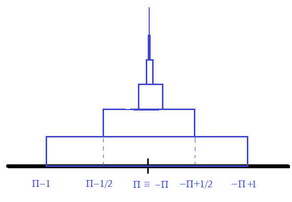
Figure 1. Function $\hat{\varphi}(t=0,\theta)-1$ in $(\pi-1,\pi)$ and in $(-\pi,-\pi+1)$ (it would have infinite “steps” do that it diverges in $\theta=\pm\pi$). For $t=-1$, only the first step would appear, and a new $m$-th step would be included at each $t=-1/m$, $m\in\mathds{N}$.

Example 4.1.

(Explicit $\varphi$). In order to give a construction of $\varphi$, start with:

$$\hat{\varphi}(t,\theta):=1+\sum_{k=1}^{\hbox{\tiny{m=Int}}[-1/t]}e^{k}\chi_{]-\pi,-\pi+\frac{1}{k}]\cup[\pi-\frac{1}{k},\pi[}(\theta)\qquad\forall t<0,\;\;\theta\in]-\pi,\pi[,$$

where Int$[-1/t]$ denotes the integer part of $-1/t$ and $\chi$ is the characteristic function of the corresponding set (equal to 1 on $]-\pi,-\pi+\frac{1}{k}]\cup[\pi-\frac{1}{k},\pi[$ and 0 otherwise), see Fig. 1. This function satisfies all the requirements but smoothness in its domain. In particular, $\hat{\varphi}$ can be continuously extended to $(t,e^{i\pi})$ when $t<0$ and to the region $t\geq 0$ as in (17).

So, $\varphi$ can be chosen by smoothing $\hat{\varphi}$ ensuring: (a) it is non- decreasing with $t$, (b) it satisfies, say, $\hat{\varphi}\leq\varphi\leq\hat{\varphi}+1$ and (c) it remains invariant under $\theta\mapsto-\theta$. These properties can be ensured by using a natural bump function to smooth each new summand, whenever $t=-1/m$.

Remark 4.2.

It is worth emphasizing that the conditions imposed for $\varphi$ are sufficient for our purposes but they are not optimized (recall the discussion in footnote 7). Indeed, the different approach in [19] implies that, for any function $\ell(t)$ which is smooth and satisfies $0<\ell(t)<\infty$ for $t<0$ and joins continuosly $\ell(t)=\infty$ for $t\geq 0$, the choice

$$\varphi(t,\theta)=\frac{1+\tan^{2}(\theta/2)}{1+\frac{4\pi^{2}}{\ell(t)^{2}}\tan^{2}(\theta/2)}$$

will also work, even if it does not fit exactly under our conditions. Although such an optimization is possible, our hypotheses may be enough to understand the qualitative behaviour of the model or to make rough estimates on cases such as the inflationary one.

Definition 4.3.

A basic cosmological topological change model (BCTCM) is the manifold

$$B=\left(\mathds{R}\times\mathds{S}^{1}\right)\setminus\{(t,e^{i\pi}):t\geq 0\}$$

endowed with a metric $g_{B}$ as in (14) with $\varphi$ satisfying the hypotheses (a), (b) and (c) therein, and continuously (then, smoothly) extended to $e^{i\pi}$ when $t<0$.

Recapitulating, we have:

1. From the topological viewpoint, $B$ is a cylinder, i.e., homeomorphic to $\mathds{R}\times\mathds{S}^{1}$.

2. The metric $g_{B}$ is smooth on the whole $B$.

3. Each slice $\{t=t_{0}\}$ is isometric to $\mathds{R}$ when $t_{0}\geq 0$ and to a cylinder of length $\ell(t_{0})<\infty$ when $t_{0}<0$, being $\lim_{t_{0}\rightarrow 0}\ell(t_{0})=\infty$.

4. For $t\geq 0$ one has (recall (17) and (18)):

   $$g=-dt^{2}+\varphi^{2}_{0}(\theta)d\theta^{2}=-dt^{2}+dx^{2},\qquad x\in\mathds{R},$$ (19)

   the latter taking as a new coordinate $x(\theta)=\int_{0}^{\theta}\varphi_{0}(\bar{\theta})d\bar{\theta},\forall\theta\in]-\pi,\pi[$.

Proposition 4.4.

Any BCTCM is globally hyperbolic, with Cauchy hypersurfaces homeomorphic to $\mathds{S}^{1}$. The slices $t=t_{0}$ are Cauchy for $\{t_{0}<0\}$ (and they are not for $t\geq 0$).

Proof.

As $t$ is a time function, global hyperbolicity follows by proving that $J^{+}(p)\cap J^{-}(q)$ is compact for any $p,q\in B$. This is trivial if $p,q$ lie either in the region $t\geq 0$ (as it is isometric to the closed half- plane $t\geq 0$ in $\mathds{L}^{2}$ by (19)) or in the cylinder $t<0$, whose slices are Cauchy (apply for example [25, Prop. 3.1]). If $t(p)<0$ and $t(q)\geq 0$, necessarily $J^{-}(q)\cap\{t=0\}$ is compact and, thus, lies in a compact subinterval of $]-\pi,\pi[$ for $\theta$. Thus, the problem is reduced again to the case of a cylinder. ∎

Even though the proof of this theorem has been obtained from general simple arguments, it is illustrative to find explicit Cauchy hypersurfaces of $B$. The comoving observer $\gamma_{0}(t)=(t,\theta=0),t\in\mathds{R}$ can be also called the centered comoving observer as it plays a similar role as in the open cosmological case. However, the singular comoving observer $\gamma_{\pi}(t)=(t,\theta=\pi),t<0$ becomes specially interesting from the causal viewpoint. For each $t_{0}<0$, let

$$\gamma_{\pm}^{t_{0}}(t)=(t,\theta^{t_{0}}_{\pm}(t)),\qquad t\geq t_{0}$$

be the two lightlike $t$-parameterized pregeodesics starting at $\gamma_{\pi}(t_{0})$, where $\theta^{t_{0}}_{+}(t_{0})=\pi$ and $\theta^{t_{0}}_{+}(t)$ decreases with $t$ towards $0$, while $\theta^{t_{0}}_{-}(t_{0})=-\pi$ and $\theta^{t}_{-}(t)$ increases with $t$ towards $0$. Notice that, once these pregeodesics abandon a small neigborhood of $\gamma_{\pi}(t_{0})$, their coordinate $\theta$ must decrease/increase until reaching the value $0$ (as $\varphi$ is bounded in $\mathds{R}\times[-\pi+\epsilon,\pi-\epsilon]$ for any $\epsilon>0$). Moreover, they must arrive at the same point in the centered comoving  observer $\gamma_{0}(t^{\prime}_{0})$ because of the invariance of $\varphi$ under $\theta\mapsto-\theta$. Notice that the topological circle given by these two lightlike segments is $E^{+}(\gamma_{\pi}(t_{0}))$, i.e., the future horismos of $\gamma_{\pi}(t_{0})$. This is composed by the points in the causal future $\gamma_{\pi}(t_{0})$ not included in the chronological one. The causal future $J^{+}(\gamma_{\pi}(t_{0}))$ can be obtained as the union of all the comoving observers starting at $E^{+}(\gamma_{\pi}(t_{0}))$. As a consequence, $I^{+}(\gamma_{\pi}(t_{0}))$ includes the region $t\geq 0$ except at most the compact subset $K{=J^{-}(E^{+}(\gamma_{\pi}(t_{0}))\cap\{t\geq 0\}}$ (which is included in $[0,\infty)\times[-\pi+\epsilon,\pi-\epsilon]$ for some $\epsilon>0$).

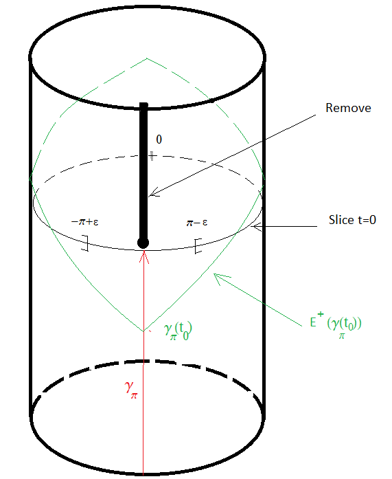
Figure 2. BCTCM, with the singular comoving observer $\gamma_{\pi}$ in red. For $t_{0}<0$, $E^{+}(\gamma_{\pi}(t_{0}))$ (in green) is a Cauchy hypersurface homeomorphic to $\mathds{S}^{1}$ which separates the spacetime in two connected open subsets. One of them is equal to $I^{+}(\gamma_{\pi}(t_{0}))$. The region $\{t\geq 0\}$ is isometric to a closed half of $\mathds{L}^{2}$, and $\{t\geq 0\}\setminus I^{+}(\gamma_{\pi}(t_{0}))$ is compact.

Summing up, from the previous discussion (see also Fig. 2)

Proposition 4.5.

In a BCTCM, the future horismos $E^{+}(\gamma_{\pi}(t_{0}))$ is a Cauchy hypersurface for any point $\gamma_{\pi}(t_{0})$, $t_{0}<0$, of the singular comoving observer.

Moreover, the chronological future $I^{+}(\gamma_{\pi}(t_{0}))$ includes the region $t\geq 0$ except a compact subset and it is foliated by the Cauchy hypersurfaces $E^{+}(\gamma_{\pi}(t))$ with $t_{0}<t<0$.

Remark 4.6.

By a Cauchy hypersurface $S$ we mean a subset which is crossed exactly once by any inextendible timelike curve (then, it is necessarily a topological hypersurface but perhaps non-smooth); indeed, $E^{+}(\gamma_{\pi}(t_{0}))$ lies exactly under these minimal hypotheses. Once such a hypersurface is obtained, general results ensure the existence of an acausal one (i.e., causal curves cannot intersect $S$ in more than a point) [13], then a smooth spacelike one [5] and, finally, a foliation of the whole spacetime by this type of Cauchy hypersurfaces [6]. Moreover, as the $t$- slices $t<0$ are Cauchy by Prop. 4.4, one can choose one of them $\Sigma$ as the initial data for the Cauchy problem. Following [7], $\Sigma$ can also be included in a Cauchy slicing (see also [23]).

However, the readers can convince theirselves that all this can be done directly in the very particular case of a BCTCM; in fact, the explicit constructions above may allow one to understand better how the model works. Notice also that the slicings are consistent with Geroch’s theorem [14] which asserts that, in any causally well behaved compact region of a spacetime limited by two disjoint compact spacelike hypersurfaces (with no boundary) $S$ and $S^{\prime}$, these two hypersurfaces, as well as any other compact spacelike one therein, must be homeomorphic.

Remark 4.7.

(1) The curvature of the metric (14) is $K=\frac{1}{\varphi}\frac{\partial^{2}\varphi}{\partial t^{2}}$ (see for example [22, Ch. 3, Prop. 44]). Taking into account that, essentially, $\varphi$ is required to grow fast with $t$ for every $\theta$ is close to $\pm\pi$ and, eventually, “stabilize” (being constant) at some $t<0$ (but not at the limit $\theta=\pm\pi$), then $\varphi$ can be chosen so that the timelike convergence condition (i.e., $K\leq 0$ in the case of surfaces) holds everywhere but close to the comoving singular observer $\gamma_{\pi}$ and small $t<0$.

(2) One could extend the definition of BCTCM by permitting that all the observers $\gamma_{\theta_{0}}(t)=(t,\theta_{0}),t<0$ are singular (in the sense of inextensible to $t=0$) for $\theta_{0}$ in an interval around $e^{i\pi}$ (i.e., $\theta_{0}\in(\pi-\delta_{0},\pi]\cup[-\pi,-\pi+\delta_{0})$, for some $\delta_{0}>0$). In principle, this case would be straightforward from the studied one, anyway, other weakenings of the hypotheses on $\varphi$ are possible (recall Remark 4.2) and might deserve a further study.

4.2. Spatial dimension $n\geq 2$

This case will be a direct extension of the previous one by using spherical coordinates $s\in(0,\pi),g_{\mathds{S}^{n-1}}$ in $\mathds{S}^{n}$ as in (1) (notice that, here, we start using $s$ instead of $r$ for the unit sphere $\mathds{S}^{n}$). However, now the topological change will imply a curvature change.

Recall that, for $n=1$, $s=|\theta|$ plays the role of the radial spherical coordinate and the pairs $\pm\theta$ play the role of a sphere, which is identifiable to $g_{\mathds{S}^{n-1}}$ when $s=1$ and collapses to a single point when $s=0,\pi$. We will use either $e^{i\pi}$ or $s=\pi$ to denote the antipodal point of $s=0$ for our choice of spherical coordinates in $\mathds{S}^{n}$.

Definition 4.8.

A basic cosmological topological and curvature change model (BCTCCM) is the manifold

$$\mathds{R}\times\mathds{S}^{n}\setminus\{(t,e^{i\pi}):t\geq 0\}$$

endowed with the metric

$$g=-dt^{2}+\varphi^{2}(t,s)ds^{2}+S_{k(t)}^{2}(r(t,s))g_{\mathds{S}^{n-1}}\qquad(t,s)\in\mathds{R}\times]0,\pi[$$ (20)

extended naturally to $s=0$, as well as to $e^{i\pi}$ when $t<0$, where:

• $\varphi$ satisfies the hypotheses (a), (b), (c) below formula (14) (including the part of (c) mentioned in footnote 7),

• $r$ is defined on $\mathds{R}\times[0,\pi]$ as:

  $$r(t,s)=\int_{0}^{s}\varphi(t,\bar{s})d\bar{s}$$

• we define $k(t)=\pi^{2}/r(t,\pi)^{2}$, in particular, $k(t)=0$ for $t\geq 0$, in agreement with (13).

Theorem 4.9.

Any BCTCCM is a smooth spacetime satisfying:

1. All the slices $t=t_{0}$ have constant curvature isometric to the sphere of extrinsic radius $r(t_{0},\pi)/\pi$, if $t_{0}<0$ and to $\mathds{R}^{n}$ otherwise.

2. It is globally hyperbolic, with Cauchy hypersurfaces homeomorphic to $\mathds{S}^{n}$. In particular, the slices $t=t_{0}<0$ are Cauchy.

Proof.

(1) By construction, $\varphi(t,s)$ was smooth; then, so is $r(t,s)$, as well as $k(t)$, the latter when $t\neq 0$. To check smoothness at $t=0$, notice that, from (16), $\sqrt{k(t)}=2\pi/\ell(t)$ and, whenever $1/|t|\leq m$ then $\ell(t)\geq 2e^{m}$. Thus,

$$\lim_{t\nearrow 0}\frac{k(t)}{|t|^{s}}=(2\pi)^{2}\lim_{t\nearrow 0}\frac{1}{|t|^{s}\ell(t)^{2}}\leq\pi^{2}\lim_{m\nearrow\infty}\frac{m^{s}}{e^{2m}}=0,$$

for all $s\in\mathds{N}$, which implies that the all $s$-th derivatives  of $k(t)$ vanish. To analize $g$, consider first the function $\varphi_{0}$ in (17) and change the coordinates $(t,s)$ by $(t,r)$ in a neighborhood of the region $t\geq 0$ so that $dr=\varphi_{0}(s)ds$ and

$$g=-dt^{2}+\varphi_{0}^{2}(s)ds^{2}+S_{k(t)}^{2}(r(t,s))g_{\mathds{S}^{n-1}}=-dt^{2}+dr^{2}+S_{k(t)}^{2}(r)g_{\mathds{S}^{n-1}}.$$ (21)

This is a smooth metric as in Theorem 2.3 and, so, the smoothness of $g$ in the whole region $(t,s)\in\mathds{R}\times]0,\pi[$ is straightforward. The required constant curvature of the $t_{0}$-slices follows from (21) when $t\geq 0$ and, otherwise, by changing the coordinate $s$ by $r(t_{0},s)$ at each slice with $t_{0}<0$. For the smoothness of the extension to $s=0$, the proof of Theorem 3.1 works with no modification as $\varphi$ is constantly equal to 1 around $s=0$ (even though this could be relaxed, recall footnote 7).

Next, let us check the smoothness of the extension of $g$ to $s=\pi$ when $t<0$. Essentially, this will also be reduced to the proof of the case $s=0$ in Theorem 3.1. For this purpose, choose $t_{1}<0$ and let $\epsilon_{0}>0$ such that $\varphi(t,s)$ is independent of $s$ around $(t_{1},\pi)$, that is,

$$\varphi_{\pi}(t):=\varphi(t,\pi)=\varphi(t,s),\qquad\forall t\in[t_{1}-\epsilon_{0},t_{1}+\epsilon_{0}],\quad\forall s\in[s_{0}:=\pi-\epsilon_{0},\pi].$$

Then, in this region define:

$$r(t,s)=\int_{0}^{s}\varphi(t,\bar{s})d\bar{s}=r(t,\pi)-\varphi_{\pi}(t)(\pi-s),\qquad\hbox{when}\;s_{0}<s\leq\pi.$$ (22)

Let us introduce the functions $\bar{s}=\pi-s$ and $\bar{r}(t,s)=r(t,\pi)-r(t,s)$. We have just to prove the smoothness $g$ (given by (20)) in coordinates $(t,\bar{r})$ at $\bar{r}=0$ (i.e., $\bar{s}=0$). Using (22),

$$\bar{r}(t,s)=\varphi_{\pi}(t)(\pi-s)=\varphi_{\pi}(t)\bar{s},\qquad d\bar{r}=\varphi_{\pi}(t)d\bar{s}+\dot{\varphi}_{\pi}(t)\bar{s}dt,$$

where $\dot{\varphi}_{\pi}$ denotes derivative, and we have

$$\varphi(t,s)^{2}ds^{2}=\varphi_{\pi}(t)^{2}d\bar{s}^{2}=d\bar{r}^{2}+\frac{\dot{\varphi}_{\pi}(t)^{2}}{\varphi_{\pi}(t)^{2}}\bar{r}^{2}dt^{2}-\frac{\dot{\varphi}_{\pi}(t)}{\varphi_{\pi}(t)}2\bar{r}d\bar{r}dt.$$ (23)

As $\bar{s}^{2}$ is a smooth function in our region, so is $\bar{r}^{2}$ as well as $\bar{r}d\bar{r}=d(\bar{r}^{2}/2)$. Substituting (23) in (20), the last two terms in (23) become irrelevant for the smoothness of $g$. So, the problem reduces to check the smoothness at $\bar{r}=0$ of the terms

$$d\bar{r}^{2}+S_{k(t)}(r(t,s))g_{\mathds{S}^{n-1}}$$ (24)

where the function $S_{k(t)}(r(t,s))$ must be expressed in the coordinates $(t,\bar{r})$. Using the expressions of $S_{k}$, $k(t)$ for a BCTCCM and $\bar{r}(t,s)$ above:

$$\begin{array}[]{rl}S_{k(t)}(r(t,s))=&\frac{r(t,\pi)}{\pi}\sin\left(\pi\,\frac{r(t,s)}{r(t,\pi)}\right)=\frac{r(t,\pi)}{\pi}\sin\left(\pi\,\left(1-\frac{\bar{r}(t,s)}{r(t,\pi)}\right)\right)\\ =&\frac{r(t,\pi)}{\pi}\sin\left(\pi\,\frac{\bar{r}(t,s)}{r(t,\pi)}\right)=S_{k(t)}(\bar{r}(t,s)).\end{array}$$ (25)

That is, $S_{k(t)}(r(t,s))$ becomes $S_{k(t)}(\bar{r})$ and the smoothness of (24) follows from Theorem 3.1.

(2) All the arguments in Prop. 4.4 can be applied for this part. In particular, applying (21), (13), the metric in the region $t\geq 0$ becomes

$$g=-dt^{2}+\varphi^{2}_{0}(s)ds^{2}+r^{2}(s)g_{\mathds{S}^{n-1}}=-dt^{2}+dr^{2}+r^{2}g_{\mathds{S}^{n-1}}$$ (26)

with $r(s)=\int_{0}^{s}\varphi_{0}(\bar{s})d\bar{s}\in]0,\infty[$, which is isometric to the standard half space $t\geq 0$ in ${\mathbb{L}}^{n+1}$. So, for any point $q$ with $t(q)\geq 0$, necessarily $J^{-}(q)\cap\{t=0\}$ is compact. Then, the slices $t=t_{0}<0$ (which are homemorphic to a sphere) are Cauchy, and those with $t_{0}\geq 0$ (homemorphic to $\mathds{R}^{n}$) cannot. ∎

Remark 4.10.

Recall that the BCTCCM metric (20) is more general than the original one in Theorem 2.3, because if the coordinate $s$ is replaced by $r(t,s)$ on the whole spacetime then additional cross terms (as in (23)) may appear. However, this can be done just around the comoving singular observer, Rem. 4.7.

4.3. Further transitions

Once the BCTCCM has been constructed, one can combine it directly with the open model to obtain a smooth transition from positive to negative curvature, namely: (i) choose a smooth function $k(t)$ with, say, $k(t)>0$, if $t<0$, and $k(t)<0$ if $t>0$, (ii) in the region $t\leq 0$ choose the metric of the BCTCCM in Defn. 4.8, (iii) in the region $t>0$ choose the metric of the open cosmological model in Theorem 3.1 with the following caution: rewrite this metric by using the coordinate $s$ and the function $\varphi_{0}$ in (26) (so that it will match smoothly with the BCTCCM at $t=0$). It is worth pointing out, about this procedure:

1. The change of coordinates in the step (iii) rellabels the comoving observers, but these observers are not modified by such a change (simply, the coordinates $r$ is changed into $s$, and the coordinate $t$ is not involved in such a change).

2. Such a model with strict transition from $k(t)<0$ to $k(t)>0$ is again globally hyperbolic with compact Cauchy hypersurfaces. Indeed, one can reason this as in the proof of Theorem 4.9 and Prop. 4.4.

   However, the following more straightforward reasoning holds. As argued in the proof of Theorem 3.1, the cones of the constructed model in $t>0$ are narrower than those of $\mathds{L}^{n+1}$ spacetime (in the chosen coordinates) and, morever, $\mathds{L}^{n+1}$ is the metric of the original BCTCCM in this region. Thus, the Cauchy hypersurfaces and foliations obtained for the BCTCCM in §4.2 remain Cauchy for the strict transition here.

3. The fact that each slice $\{t=t_{0}\}$ was a Cauchy hypersurface for $t_{0}<0$ but it is only a partial Cauchy one for $t_{0}>0$ becomes geometrically evident. However, this might not be evident for the comoving observers. In fact, these slices are associated with their restspaces. The infinitesimal and, eventually, local measures of these spaces may be achieved as a consequence of the principle of equivalence, but it is not straightforward how to make global measurements. Recall that the “disappearance” of the singular comoving observer cannot be seen directly by any (comoving or not) observer, as the spacetime is globally hyperbolic and, thus, free of naked singularities.

As commented in the Introduction and Rem. 2.4, the possibility of the existence of a spacetime in which the topology of certain geometrically preferred sections is changing in time have been considered some times in the literature. The starting point was Stephani’s study of the class of spacetimes embeddable in a flat five-dimensional space [28] (see also [29, Chapter 15]), which included the now so-called Stephani Universes [18]. Especially, Krasiński and later Sussman developed both the local [16, 30] and the global viewpoints [17, 31] (see also the short overview in [17, p. 675] and the book [18]). However, their viewpoint is different to ours.

In the case of Krasiński [16, 17], de Sitter 4-spacetime serves as the qualitative model for the curvature sign changing foliations (see [17]). The leaves of the foliation are not the slices of the original universal time $t$ in (7) (which is generically a priviledged time function, in a similar way as the FLRW case); thus, the leaves are not orthogonal to the comoving observers at $\partial_{t}$. Moreover, the coordinate $r$ is considered globally and, as pointed out in Remark 2.4 (2) (see also the Appendix), this may introduce smoothability issues. Sussman [30, 31] considered an expression of the 4-metric which separates the cases of positive, negative and zero spatial curvature (see formulas (1) and (2) in these references) and he studied systematically the cases of one, two or zero comoving centers permitted by $O(3)$ symmetry. In comparison, our direct approach gives a straight geometric picture where both global hyperbolicity and an explicit Cauchy slicing emerge naturally.

Other topological transitions between spatially compact and non-compact universes as those in [15, §5.2] are quite different to ours.

5. Conclusions

We have carried out a direct study of a class of simple cosmological models (related to a more general class of spacetimes studied in dimension 4 by Stephani [28, 29]) with a universal time function $t$ giving rise to freely following comoving observers whose restspaces $\{t=t_{0}\}$ have constant curvature $k(t_{0})$ and vary with $t_{0}$, this variation including its sign. We have focused on a rigurous mathematical presentation of the models, which permit a direct comparison with usual hypotheses on isotropy and homogeneity. From the local viewpoint, this includes a detailed study of the regularity of the metric. From the global one, our models are globally hyperbolic spacetimes and we have found two natural classes. The open models ($k(t)\leq 0$ everywhere) have a simple intuitive global structure. They distinguish a centered comoving observer which, in certain sense, is the center of the spatial expansion or contration governed by $k(t)$. The closed models ($k(t)>0$ somewhere) are much subtler globally. This happens because the $t$-slices must present a topology change (from $\mathds{S}^{n}$ when $k(t)>0$ to $\mathds{R}^{n}$), which has to be compatible with the rigid product topological structure of any globally hyperbolic spacetime (that is, the topology $\mathds{R}\times\Sigma$, where $\Sigma$ is any Cauchy hypersurface). In a natural way, this leads to the existence of a singular comoving observer $\gamma_{\pi}$ (in addition to the previous centered one). From the global viewpoint, this is the truly priviledged observer, as it makes apparent the Cauchy splitting; in fact, the centered observer can be regarded only as the “farthest” one at each $t$-slice (see footnote 10).

These models release some possibilities which might fit in current Cosmology. For example, the open models are consistent with a flat space at some “universal instant” $\{t=t_{0}\}$ and a bouncing therein (Ex. 3.4, footnote 6). The closed ones might apply to inflationary processes along the singular comoving observer $\gamma_{\pi}$, which become the key for both, the spatial topology change and the center of the expansion. In fact, $\gamma_{\pi}$ lies in the region $t<0$ of the time function $t$ associated with the constant curvature slices, but the spacetime has no naked singularites. So, the singular comoving observer will “live” for every instant of any Cauchy time function, as any other (inextendible) observer. These features might attract the attention of the community and give rise to observational issues (recall [11, 12]) to be studied further.

Data Availability and conflict of interest statements

Data sharing is not applicable to this article as no datasets were generated or analysed during the current study.

The author states that there is no conflict of interest.

Appendix: expression of the Ricci tensor

The computation of the Ricci tensor of the fundamental metric in Theorem 2.3 can be carried out by using its warped structure as in [22, Corollary 7.43]. Indeed, for $X,Y\in$ Span$\{\partial_{t},\partial_{r}\}$ one has:

$$\hbox{Ric}(X,Y)=-\frac{n}{S_{k(t)}(r)}\hbox{Hess}(S(t,r))(X,Y)$$

with $S(t,r)$ as in (3) with Hessian expressable in terms of the one of $S_{k}(r)$:

$$\begin{array}[]{rlll}\partial_{r}S_{k}(r)=C_{k}(r)&&&\partial_{k}S_{k}(r)=\frac{1}{2k}(rC_{k}(r)-S_{k}(r))\\ \partial_{r}^{2}S_{k}(r)=-kS_{k}(r)&&&\partial_{rk}^{2}S_{k}(r)=-\frac{r}{2}S_{k}(r)\end{array}$$

$$\begin{array}[]{l}\partial_{k}^{2}S_{k}(r)=\frac{1}{4k^{2}}\left(-3rC_{k}(r)+(3-kr^{2})S_{k}(r)\right),\end{array}$$

(notice $\partial_{k}C_{k}(r)=-rS_{k}(r)/2$, $\lim_{k\rightarrow 0}\partial_{k}S_{k}(r)=-r^{3}/6$, $\lim_{k\rightarrow 0}\partial^{2}_{k}S_{k}(r)=r^{5}/60$). Thus, $\partial_{t}S(t,r)=k^{\prime}(t)\partial_{k}S_{k(t)}(r)$ and:

$$\begin{array}[]{llll}\partial_{r}^{2}S(t,r)=-k(t)S_{k(t)}(r)&&&\partial_{rt}^{2}S(t,r)=-\frac{k^{\prime}(t)r}{2}S_{k(t)}(r)\end{array}$$

$$\begin{array}[]{l}\partial_{tt}^{2}S(t,r)=\frac{2k(t)k^{\prime\prime}(t)-3k^{\prime}(t)^{2}}{4k(t)^{2}}(rC_{k(t)}(r)-S_{k(t)}(r))-\frac{k^{\prime}(t)^{2}}{4k(t)}r^{2}S_{k(t)}(r)\end{array}$$

So, the Ricci tensor for the base of the warped product is:

$$\begin{array}[]{llll}\hbox{Ric}(\partial_{r},\partial_{r})=nk(t)&&&\hbox{Ric}(\partial_{r},\partial_{t})=\frac{n}{2}k^{\prime}(t)r\end{array}$$

$$\begin{array}[]{l}\hbox{Ric}(\partial_{t},\partial_{t})=-n\frac{2k(t)k^{\prime\prime}(t)-3k^{\prime}(t)^{2}}{4k(t)^{2}}(\frac{r}{T_{k(t)}(r)}-1)+n\frac{k^{\prime}(t)^{2}}{4k(t)}r^{2}\end{array}$$

Now, if $V,W$ are vectors tangent to the fiber $(S^{n-1},g_{\mathds{S}^{n-1}})$ one has Ric$(X,V)=0$ (as in any warped product) and

$$\hbox{Ric}(V,W)=[(n-1)-S\Delta S+(n-2)dS(\hbox{grad}(S))]\;g_{\mathds{S}^{n-1}}(V,W)$$

where $\Delta S$, $\hbox{grad}(S)$ denote, resp., the Laplacian and gradient of $S(t,r)$ for the metric $-dt^{2}+dr^{2}$, thus:

$$\begin{array}[]{rl}dS(\hbox{grad}(S))=&-\frac{k^{\prime}(t)^{2}}{4k^{2}}(rC_{k}(r)-S_{k}(r))^{2}+C_{k}(r)^{2}\\ \Delta S=&-\frac{2k(t)k^{\prime\prime}(t)-3k^{\prime}(t)^{2}}{4k(t)^{2}}(rC_{k(t)}(r)-S_{k(t)}(r))+\frac{k^{\prime}(t)^{2}r^{2}-4k(t)^{2}}{4k(t)}S_{k(t)}(r).\end{array}$$

References

- [1] U. Abresch, D. Gromoll. On complete manifolds with nonnegative Ricci curvature. J. Amer. Math. Soc. 3 (1990), no. 2, 355-374.
- [2] L.J. Alías, A. Romero, M. Sánchez. Uniqueness of complete spacelike hypersurfaces of constant mean curvature in generalized Robertson-Walker spacetimes. Gen. Relativity Gravitation 27 (1995), no. 1, 71–84.
- [3] R. Ávalos. On the Rigidity of Cosmological Space-times. Arxiv-preprints, arXiv:2211.07013 (2022).
- [4] J. K. Beem, P. E. Ehrlich, K. L. Easley. Global Lorentzian geometry, volume 202 of Monographs and Textbooks in Pure and Applied Mathematics. Marcel Dekker, Inc., New York, Second Edition, 1996.
- [5] A. N. Bernal, M. Sánchez. On smooth Cauchy hypersurfaces and Geroch’s splitting theorem. Comm. Math. Phys. 243 (2003), no. 3, 461-470.
- [6] A. N. Bernal, M. Sánchez. Smoothness of time functions and the metric splitting of globally hyperbolic spacetimes. Comm. Math. Phys. 257 (2005) , no. 1, 43-50.
- [7] A. N. Bernal, M. Sánchez. Further results on the smoothability of Cauchy hypersurfaces and Cauchy time functions. Lett. Math. Phys. 77 (2006), no. 2, 183.197.
- [8] S.M. Carroll: An Introduction to General Relativity, San Francisco: Addison-Wesley (2004).
- [9] I. Chavel. Riemannian geometry. A modern introduction. Cambridge Studies in Advanced Mathematics, 98. Cambridge University Press, Cambridge (2006).
- [10] Y. Choquet-Bruhat, General Relativity and the Einstein Equations (Oxford Mathematical Monographs), Oxford (2008).
- [11] G. F. R. Ellis. Is the universe expanding? Gen. Relat. Gravit. 9 (1978) 87-94.
- [12] G. F. R. Ellis. The homogeneity of the universe. Gen. Relat. Gravit. 11 (1979) 281-289.
- [13] R. Geroch. Domain of dependence J. Math. Phys. 11 (1970) 437-449.
- [14] R. Geroch. Topology in general relativity. J. Math. Phys. 8 (1967) 782-786.
- [15] M. Y. Konstantinov, V. N. Melnikov. Topological transitions in the theory of spacetime. Class. Quantum Grav. 3 (1986) 401-416.
- [16] A. Krasiński. Space-times with spherically symmetric hypersurfaces Gen. Relat. Gravit. 13 (1981) 1021-1035.
- [17] A. Krasiński. On the Global Geometry of the Stephani Universe Gen. Relat. Gravit. 13 (1983) 674-689.
- [18] A. Krasiński. Inhomogeneous cosmological models Cambridge University Press, Cambridge (1997).
- [19] M. Mars, R. Vera, in progress (2022).
- [20] S. Hawking, G. Ellis. The Large Scale Structure of Space-Time (Cambridge Monographs on Mathematical Physics). Cambridge: Cambridge University Press (1973).
- [21] C.W. Misner, K.S. Thorne, J.A. Wheeler. Gravitation, W. H. Freeman, Princeton University Press (1973).
- [22] B. O’Neill. Semi-Riemannian geometry. Academic Press, Inc. New York (1983).
- [23] H. Ringström. The Cauchy problem in general relativity. ESI Lectures in Mathematics and Physics. European Mathematical Society (EMS), Zürich (2009).
- [24] R.K. Sachs, H. Wu. General Relativity and Cosmology. Bull Amer. Math. Soc., Vol. 83, N. 6 (1977).
- [25] M. Sánchez. Globally hyperbolic spacetimes: slicings, boundaries and counterexamples. Arxiv preprints, arxiv:2110.13672.
- [26] W. Rossmann. Lie Groups An Introduction Through Linear Groups. Oxford Graduate Texts in Mathematics (2002).
- [27] M. Sánchez. On the geometry of generalized Robertson-Walker spacetimes: geodesics. Gen. Relat. Gravit. 30 (1998), no. 6, 915-932.
- [28] H. Stephani. Über Lösungen der Einsteinschen Feldgleichungen, die sich in einen fünfdimensionalen flachen Raum einbetten lassen. Comm. Math. Phys. 4 (1967), no. 2, 137-142.
- [29] H. Stephani, D. Kramer, M. MacCallum, C. Hoenselaers, & E. Herlt. Exact Solutions of Einstein’s Field Equations (2nd ed., Cambridge Monographs on Mathematical Physics). Cambridge University Press (2003).
- [30] R. A. Sussman. On spherically symmetric shear-free perfect fluid configurations (neutral and charged). II. Equation of state and singularities J. Math. Phys. 29, (1988) 945-970.
- [31] R. A. Sussman. On spherically symmetric shear-free perfect fluid configurations (neutral and charged). III. Global view J. Math. Phys. 29 (1988) 1177-1211.
- [32] R.M. Wald. General Relativity. The University of Chicago Press, Chicago (1984).
- [33] S. Weinberg. Gravitation and Cosmology: Principles and Applications of the General Theory of Relativity, John Wiley & Sons, N.Y. (1972).