Aggregation Methods for Computing Steady-States in Statistical Physics

Abstract.

We give a new proof of local convergence of a multigrid method called iterative aggregation/disaggregation (IAD) for computing steady-states of Markov chains. Our proof leads naturally to precise and interpretable estimates of the asymptotic rate of convergence. We study IAD as a model of more complex methods from statistical physics for computing nonequilibrium steady-states, such as the nonequilibrium umbrella sampling method of Warmflash, et al. We explain why it may be possible to use methods like IAD to efficiently calculate steady-states of processes in statistical physics and how to choose parameters to optimize efficiency.

1. Introduction

We prove local convergence of iterative aggregation/disaggregation (IAD) for computing steady-states of Markov chains, and we estimate the asymptotic rate of convergence. IAD was devised in the 1960’s to solve economic input-output models; see the references given in [20, 33]. Substantially equivalent methods were independently developed in the 1980’s to calculate steady-states of Markov chains [14, 4, 13, 3]. In the 2000’s, similar ideas arose for a third time as part of more complex methods for calculating nonequilibrium steady-states and reaction rates in statistical physics [35, 34, 2, 1, 9, 10]. We study IAD as a simple model of these complex methods. We explain why it may be possible to use methods like IAD to efficiently calculate steady-states in statistical physics and how to choose parameters to optimize efficiency. We hope others will apply our results to understand IAD in other contexts.

We call a Markov process nonequilibrium if it is irreversible. A physical system subject to nonconservative forces or external flows of energy and matter would typically be modeled by a nonequilibrium process, e.g. a single-molecule experiment where a protein is subjected to a flow of ions [19, 8]. In principle, to sample the steady-state distribution of any ergodic process, reversible or irreversible, one can take the average over a long trajectory. In practice, however, trajectory averages converge to the steady-state very slowly when obstacles like bottlenecks inhibit exploration of the state space. For example, a process modeling a protein may spend most of the time vibrating around some stable folded state, undergoing transitions between different folded states only rarely. Such a process is said to be metastable.

Computing the steady-state of a metastable, nonequilibrium process is especially difficult. Reliable methods have been devised to efficiently compute steady-states of reversible, metastable processes, e.g. parallel tempering [30, 11], umbrella sampling [32, 16, 29], metadynamics [17], and adaptive biasing [5]. These methods are essential tools for simulating systems in equilibrium. Unfortunately, however, none of them can compute nonequilibrium steady-states. Each requires either reversibility or knowledge of the steady-state density, and when computing nonequilibrium steady-states one typically knows only the generator of the process. By constrast, in equilibrium, the steady-state has the Boltzmann density, which can almost always be calculated up to a normalizing constant.

Recently, analogous methods have been devised to compute nonequilibrium steady-states and dynamical quantities such as reaction rates. We consider one class derived from umbrella sampling, including nonequilibrium umbrella sampling (NEUS) [35], trajectory parallelization and tilting [34], weighted ensemble with a direct solve [2], exact milestoning [1], trajectory stratification [9], and injection measures [10]. The exact objectives and details of these methods differ significantly, but they are all essentially stochastic evolving particle systems that approximate IAD (or a similar deterministic dynamics) in the limit of a large number of particles. We refer to [10] for details. We ask whether approximating IAD is a suitable goal for an algorithm designed to compute steady-states in statistical physics.

IAD is like an algebraic multigrid method, but it is nonlinear and nonsymmetric which significantly complicates its analysis, cf. Appendix D.3. In the earliest convergence analysis of IAD known to us, Mandel and Sekerka proved local convergence for a class of problems including the solution of input-output models but not steady-states of Markov chains [20]. Later work verified local convergence for Markov chains under various conditions and for various versions of the IAD algorithm [24, 15, 21, 22, 23, 10]. We are not aware of a proof of global convergence that holds under general conditions. However, see [23] for a proof of global convergence under somewhat restrictive conditions and examples where IAD fails to converge. The efficiency of IAD has been studied in special cases, including nearly completely decomposable chains [14] and cyclic chains [28].

We contribute a new proof of local convergence of IAD under weak conditions that are easy to verify. The usual conditions that guarantee convergence of a Markov chain to a steady-state, irreducibility and aperiodicity, do not suffice to prove even local convergence of IAD, cf. Appendix B.2 and [23]. If $P$ is the transition matrix of the chain, we prove local convergence when $P$ and $P^{\mathrm{t}}P$ are irreducible, cf. Theorem 2. It is equivalent to assume that the chain is strictly contracting in a certain norm, cf. Lemma 3. A sufficient condition is that $P$ be irreducible and have positive diagonal.

Our proof of local convergence leads to precise and interpretable estimates of the asymptotic rate of convergence, cf. Theorem 3 and Corollary 1. Based on these estimates, we have developed some general advice to guide the choice of parameters in IAD; see the discussion following Corollary 1. We apply our theory of the rate of convergence in Section 6 to explain why it may be possible to use methods like IAD to efficiently compute steady-states of reversible or irreversible processes arising in statistical physics and computational chemistry. To be precise, in Section 6, we introduce a family of Markov chains analogous to the metastable diffusion processes that are widely used as models of molecular systems. We then explain why IAD can sometimes efficiently calculate the steady-states of such chains and how to choose the parameters in practice. We illustrate our conclusions with numerical experiments. We developed our rate estimates with these examples from statistical physics in mind, but our results are general, and we hope others will apply them to understand IAD in other contexts.

2. Notation

Here, we summarize our notation. Notation is also explained below when it first appears.

• $P\in\mathbb{R}^{N\times N}$ will be an irreducible, column stochastic transition matrix with invariant distribution $\mu\in\mathbb{R}^{N}$.

• For any matrix or vector $M$, $M\geq 0$ means all entries of $M$ are nonnegative. $M>0$ means all entries are positive.

• $\mathds{1}$ will denote a vector of all ones and $I$ will denote the identity matrix. The dimension of $\mathds{1}$ or $I$ will be determined by the context.

• For any $A\subset\{1,\dots,N\}$, $\mathds{1}_{A}$ will denote the characteristic function of $A$. That is, $\mathds{1}_{A}(x)=1$ if $x\in A$ and $\mathds{1}_{A}(x)=0$ if $x\notin A$.

• For any vector $\nu\in\mathbb{R}^{k}$, we let $\operatorname{diag}(\nu)\in\mathbb{R}^{k\times k}$ denote the diagonal matrix with $\operatorname{diag}(\nu)_{ii}=\nu_{i}$ for $i=1,\dots,k$.

• $\lVert\cdot\rVert_{\nu}$ and $\langle,\rangle_{\nu}$ denote the $\ell^{2}(\nu)$-norm and inner product, respectively; see Definition 5. For $M\in\mathbb{R}^{k\times k}$, $M^{\ast,\nu}$ denotes the adjoint of $M$ with respect to the $\ell^{2}(\nu)$-inner product. In some proofs, we simplify notation, letting $\lVert\cdot\rVert$, $\langle,\rangle$, and $M^{\ast}$ denote the $\ell^{2}(1/\mu)$-norm, inner product, and adjoint, respectively.

• For any operator $M\in\mathbb{R}^{M\times M}$, $\operatorname{Rg}(M)$ denotes the range of $M$.

3. The Iterative Aggregation/Disaggregation Method

Iterative Aggregation/Disaggregation (IAD) is a numerical method for computing the steady-state distribution of a Markov chain. Let $P\in\mathbb{R}^{N\times N}$ be the column stochastic transition probability matrix of a discrete-time Markov chain on the state space

$$\Omega=\{1,\dots,N\}.$$

We call $\Omega$ the fine space. We assume that $P$ is irreducible, so there is a unique steady-state probability vector $\mu\in\mathbb{R}^{N}$ solving

$$P\mu=\mu.$$

In each step of IAD, one calculates a coarse approximation to $P$ based on a user-specified partition of $\Omega$ into disjoint sets $\{S_{i}:i=1,\dots,n\}$. We call each set $S_{i}$ a coarse state, and we call the set $\{1,\dots,n\}$ of indices the coarse space. To define the coarse approximation, we specify operators mapping between the sets of probability vectors on the fine and coarse spaces. The aggregation operator maps vectors on the fine space to vectors on the coarse space.

Definition 1.

We define the aggregation operator $A:\mathbb{R}^{N}\rightarrow\mathbb{R}^{n}$ by

$$(A\nu)_{i}:=\nu^{\mathrm{t}}\mathds{1}_{S_{i}}=\sum_{x\in S_{i}}\nu_{x}$$

for any $i=1,\dots,n$ and $\nu\in\mathbb{R}^{N}$.

Note that when $\nu$ is a probability vector, $A\nu_{i}$ is simply the probability of $S_{i}$ under $\nu$. Moreover, if $\nu$ is a probability vector, then so is $A\nu$.

The disaggregation operator maps vectors on the coarse space to vectors on the fine space. It depends on the current approximation $\tilde{\mu}$ of the steady-state $\mu$.

Definition 2.

Given a probability vector $\tilde{\mu}\in\mathbb{R}^{N}$ with $A\tilde{\mu}>0$ and a coarse state $S_{i}$, define the conditional distribution $\tilde{\mu}(\cdot|S_{i})$ by

$$\tilde{\mu}(j|S_{i})=\frac{\tilde{\mu}_{j}\mathds{1}_{S_{i}}(j)}{A\tilde{\mu}_{i}}$$

for $j\in\Omega$. Here, $\mathds{1}_{S_{i}}$ denotes the characteristic function of $S_{i}$. Define the disaggregation operator $D(\tilde{\mu}):\mathbb{R}^{n}\rightarrow\mathbb{R}^{N}$ by

$$D(\tilde{\mu})z_{j}:=\sum_{i=1}^{n}z_{i}\tilde{\mu}(j|S_{i})$$

for any $z\in\mathbb{R}^{n}$.

Note that if $z$ is a probability vector, so is $D(\tilde{\mu})z$. Also, observe that $D(\tilde{\mu})$ is defined only when $A\tilde{\mu}>0$. This will always be the case in practice under our assumptions, cf. Lemma 1.

Given an approximation $\tilde{\mu}$ of $\mu$, the coarse approximation $C(\tilde{\mu})$ to $P$ is defined by composing $P$ with $A$ and $D(\tilde{\mu})$.

Definition 3.

Let $\tilde{\mu}\in\mathbb{R}^{N}$ be a probability vector with $A\tilde{\mu}>0$. We define the coarse approximation $C(\tilde{\mu})\in\mathbb{R}^{n\times n}$ by

$$C(\tilde{\mu})=APD(\tilde{\mu}).$$

The coarse approximation $C(\tilde{\mu})$ is a column stochastic matrix. To see this, note that $C(\tilde{\mu})$ maps probability vectors to probability vectors, since each of $A$, $P$, and $D(\tilde{\mu})$ maps probability vectors to probability vectors. In each step of IAD, one solves for the steady-state of $C(\tilde{\mu})$. It is convenient to establish some general notation for this operation.

Definition 4.

For $M$ an irreducible and column stochastic matrix, we let $z(M)$ denote the unique probability vector solving

$$z(M)=Mz(M).$$

Now let $\mu^{0}\in\mathbb{R}^{N}$ be a user-specified initial approximation of $\mu$. In IAD, one alternates coarse correction and smoothing steps. Given a probability $\mu^{k}\in\mathbb{R}^{N}$, the coarse correction step is to compute

$$\mu^{k+\frac{1}{2}}=D(\mu^{k})z(C(\mu^{k})).$$ (1)

To compute $z(C(\mu^{k}))$ in practice, one can use the algorithm outlined in Appendix A or other direct methods of numerical linear algebra. The smoothing step is to compute

$$\mu^{k+1}=P\mu^{k+\frac{1}{2}}.$$ (2)

Note that the smoothing step is the same as one step of the power method for calculating $\mu$ and also the same as evolving $\mu^{k+\frac{1}{2}}$ by one step under the forwards equation for the chain.

Many variations of IAD have appeared in the literature. We will not treat all of them. Some versions apply to substochastic problems such as economic input-output models [20, 33]. Others use different smoothers [15, 24, 21], apply multiple smoothing iterations at each step [15, 24, 21], smooth the aggregation or disaggregation operators [6], use a hierarchy of several coarse approximations in a multigrid V or W-cycle [7], or solve infinite-dimensional problems using more general aggregation and disaggregation operators [24, 10]. We do not consider these possibilities.

We now summarize our assumptions and show that IAD is well-posed.

Assumption 1.

We assume:

1. $P$ is irreducible.

2. The initial approximation $\mu^{0}$ of the steady-state $\mu$ is strictly positive.

Lemma 1.

If Assumption 1 holds, then the iterates $\mu^{k}$ produced by IAD are defined for all $k\in\mathbb{N}$. In particular, $A\mu^{k}>0$ and $C(\mu^{k})$ is irreducible, so $D(\mu^{k})$ and $z(C(\mu^{k}))$ are defined.

Proof.

See Appendix B.1. ∎

If one does not assume $\mu^{0}>0$, then $C(\mu^{0})$ may be reducible, in which case the steady-state $z(C(\mu^{0}))$ need not be unique. This can occur even when $P$ is both irreducible and aperiodic; see Appendix B.2 for an example.

Finally, we present a complete version of IAD with a termination criterion similar to those typically used in practice.

Algorithm 1.

The user must specify the following:

1. A column stochastic and irreducible transition matrix $P\in\mathbb{R}^{N\times N}$.

2. A partition $\{S_{i}:i=1,\dots,n\}$ of $\{1,\dots,N\}$ into disjoint sets.

3. A probability vector $\mu^{0}\in\mathbb{R}^{N}$ with $\mu_{0}>0$.

4. An error tolerance $\tau>0$.

Given these data, IAD proceeds as follows:

1. Set $\mu^{\textrm{old}}=\mu^{0}$.

2. Calculate $z(C(\mu^{\textrm{old}}))$ using the algorithm in Appendix A. Set

   $$\mu^{\textrm{new}}=PD(\mu^{\textrm{old}})z(C(\mu^{\textrm{old}})).$$

3. If

   $$\max_{i\in 1,\dots,N}\frac{\lvert\mu^{\textrm{new}}_{i}-\mu^{\textrm{old}}_{i}\rvert}{\mu^{\textrm{old}}_{i}}\leq\tau\text{ and }\max_{i\in 1,\dots,N}\frac{\lvert P\mu^{\textrm{new}}_{i}-\mu^{\textrm{new}}_{i}\rvert}{P\mu^{\textrm{new}}_{i}}\leq\tau,$$

   then output $\mu^{\textrm{new}}$. Otherwise, set $\mu^{\textrm{old}}=\mu^{\textrm{new}}$, and return to step (2) above.

4. Local Convergence of IAD

In this section, we prove local convergence of IAD. That is, we show that if the initial approximation $\mu^{0}$ is sufficiently close to the true steady-state $\mu$, then $\mu^{k}$ converges to $\mu$. We begin with an analysis of the smoothing step of IAD in Section 4.1, which is the power method. In Section 4.2, we prove local convergence of IAD.

4.1. The Power Method

Here, we prove convergence of the power method (or equivalently convergence of the forwards equation of the chain) to the steady-state $\mu$. Of course, convergence of the power method is already well-understood. The details of our particular proof will be instrumental in our analysis of the efficiency of IAD, however. We begin by defining convenient norms.

Definition 5.

Let $\nu\in\mathbb{R}^{k}$ with $\nu>0$. We define the $\ell^{2}(\nu)$-norm and inner product by

$$\langle x,y\rangle_{\nu}=\sum_{i=1}^{k}x_{i}y_{i}\nu_{i}\text{ and }\lVert x\rVert_{\nu}=\langle x,x\rangle_{\nu}^{\frac{1}{2}},$$

for $x,y\in\mathbb{R}^{k}$. Given $M\in\mathbb{R}^{k\times k}$, we let $\lVert M\lVert_{\nu}$ denote the induced operator norm. We let $M^{\ast,\nu}$ be the adjoint matrix so that

$$\langle Mx,y\rangle_{\nu}=\langle x,M^{\ast,\nu}y\rangle_{\nu}$$

for all $x,y\in\mathbb{R}^{k}$.

We will use the $\ell^{2}(1/\mu)$-norm to measure discrepancies between probability measures on $\Omega$, for example the error $\mu^{k}-\mu$ after $k$ steps of IAD. The $\ell^{2}(\mu)$-norm will arise when we analyze the efficiency of IAD. As a first step in our analysis of the power method, we relate adjoints in the $\ell^{2}(1/\mu)$-inner product to time reversals.

Lemma 2.

Let $P\in\mathbb{R}^{N\times N}$ be column stochastic and irreducible. The time reversal of $P$ is $P^{\ast,1/\mu}$. In particular,

$$P^{\ast,1/\mu}=\operatorname{diag}(\mu)P^{\mathrm{t}}\operatorname{diag}(1/\mu)$$ (3)

is column stochastic, irreducible, and has invariant distribution $\mu$.

Proof.

See Appendix C.1. ∎

The spectrum of the operator $P^{\ast,1/\mu}P$ will play a crucial role in our proof of convergence of the power method and in our efficiency analysis of IAD. By Lemma 2, $P^{\ast,1/\mu}P$ is column stochastic with invariant distribution $\mu$. Therefore, $\mathds{1}$ is a left eigenvector of $P^{\ast,1/\mu}P$ with eigenvalue $1$, and $\mu$ is the corresponding right eigenvector. (Here, $\mathds{1}\in\mathbb{R}^{N}$ denotes the vector whose entries are all equal to one.) Moreover, $P^{\ast,1/\mu}P$ is self-adjoint and positive semidefinite with respect to the $\ell^{2}(1/\mu)$-inner product. Therefore, $\sigma(P^{\ast,1/\mu}P)\subset[0,1]$. Let

$$1=\lambda_{1}\geq\lambda_{2}\geq\dots\geq\lambda_{N}\geq 0$$

be the eigenvalues of $P^{\ast,1/\mu}P$ listed in decreasing order and with repetition if any have multiplicity greater than one. Let $v_{1},\dots,v_{N}$ be the corresponding right eigenvectors. Since $P^{\ast,1/\mu}P$ is self-adjoint, we may assume that the eigenvectors are an orthonormal basis of $\mathbb{R}^{N}$ with the $\ell^{2}(1/\mu)$-inner product, so

$$\langle v_{i},v_{j}\rangle_{1/\mu}=\delta_{ij},$$

and we have the diagonalization

$$P^{\ast,1/\mu}P=\mu\mathds{1}^{\mathrm{t}}+\sum_{k=2}^{N}\lambda_{k}v_{k}v_{k}^{\mathrm{t}}\operatorname{diag}(1/\mu).$$ (4)

We will refer to this diagonalization frequently. Note that the left eigenvectors of $P^{\ast,1/\mu}P$ are

$$v_{1}^{\prime}=\mathds{1},v_{2}^{\prime}=\operatorname{diag}(1/\mu)v_{2},\dots,v_{N}^{\prime}=\operatorname{diag}(1/\mu)v_{N}.$$

The left eigenvectors play an important role in our efficiency analysis of IAD.

We now show that when $P$ is irreducible, the power method for computing $\mu$ is strictly contracting in the $\ell^{2}(1/\mu)$-norm if and only if $P^{\mathrm{t}}P$ is irreducible.

Lemma 3.

Let $P\in\mathbb{R}^{N\times N}$ be an irreducible, column stochastic matrix. Let $\nu^{0}\in\mathbb{R}^{N}$ be a probability vector, and define the power method iteration

$$\nu^{k+1}=P\nu^{k}.$$

Define

$$\hat{P}=P-\mu\mathds{1}^{\mathrm{t}}.$$

We have

$$\nu^{k+1}-\mu=\hat{P}(\nu^{k}-\mu).$$ (5)

Moreover,

$$\lVert\hat{P}\rVert_{1/\mu}=\sqrt{\lambda_{2}},$$

and $\lambda_{2}<1$ if and only if $P^{\mathrm{t}}P$ is irreducible.

Proof.

See Appendix C.2. ∎

Note that asymptotic rate of convergence of the power method is

$$\lim_{m\rightarrow\infty}\lVert\hat{P}^{m}\rVert^{\frac{1}{m}}=\rho(\hat{P}).$$

For irreversible chains, $\rho(\hat{P})$ may be significantly less than the contraction constant $\lVert\hat{P}\rVert_{1/\mu}$ of the power method in the $\ell^{2}(1/\mu)$-norm. See Section 6.4 for an example. However, for reversible chains, we have $\rho(\hat{P})=\lVert\hat{P}\rVert_{1/\mu}$, since $\hat{P}^{\ast,1/\mu}=\hat{P}$.

In our convergence analysis of IAD, we assume that $P^{\mathrm{t}}P$ is irreducible. By formula (3) for $P^{\ast,1/\mu}$, it is equivalent to assume that $P^{\ast,1/\mu}P$ is irreducible. A sufficient, but not necessary, condition is that $P$ be irreducible with positive diagonal. We note that if $P$ is irreducible but $P^{\mathrm{t}}P$ is not, then $\bar{P}=\frac{1}{2}(I+P)$ is irreducible, has a positive diagonal, and has the same unique steady-state as $P$. Therefore, to compute the steady-state of $P$ one could apply IAD with $\bar{P}$ in place of $P$, and local convergence would then be guaranteed by the results below.

We now give an example to illustrate what can go wrong when $P^{\mathrm{t}}P$ is reducible. Consider a right shift on three states:

$$P=\begin{pmatrix}0&0&1\\ 1&0&0\\ 0&1&0\end{pmatrix}.$$

This is an irreducible Markov chain, and the steady-state is the uniform distribution $\frac{1}{3}\mathds{1}\in\mathbb{R}^{3}$. The time-reversal is the left shift $P^{\ast,\frac{1}{3}\mathds{1}}=P^{\mathrm{t}}=P^{-1}$. Therefore, $P^{\ast,\frac{1}{3}\mathds{1}}P=I$ is reducible even though both $P$ and $P^{\ast,\frac{1}{3}\mathds{1}}$ are irreducible. In this case, $\lVert\hat{P}\rVert_{1/\mu}=1$, and the power method does not converge, since $P$ is periodic.

The right shift in our last example is irreducible, but periodic. There also exist irreducible, aperiodic chains so that $P^{\mathrm{t}}P$ is reducible. For such chains, the power method is convergent, but it is not a strict contraction in the $\ell^{2}(1/\mu)$-norm. See Appendix B.2 and [23] for an example of an irreducible, aperiodic chain so that $P^{\mathrm{t}}P$ is reducible and IAD is not locally convergent.

4.2. Local Convergence of IAD

Here, we prove local convergence of IAD. We begin with a convenient reformulation of the steady-state problem for a Markov chain.

Lemma 4.

Let $M\in\mathbb{R}^{k\times k}$ be an irreducible column stochastic matrix, and let $v,w\in\mathbb{R}^{k}$ with $\mathds{1}^{\mathrm{t}}v\neq 0$ and $z(M)^{t}w\neq 0$. The matrix $I-M+vw^{\mathrm{t}}$ is invertible, and

$$z(M)=(I-M+vw^{\mathrm{t}})^{-1}vw^{\mathrm{t}}z(M).$$

Proof.

See Appendix D.1. ∎

We use two special cases of Lemma 4. First, the steady-state $\mu\in\mathbb{R}^{N}$ is the unique solution $x$ of

$$(I-P+\mu\mathds{1}^{\mathrm{t}})x=\mu.$$ (6)

Second, the coarse steady-state $z(C(\mu^{k}))\in\mathbb{R}^{n}$ is the unique solution of

$$(I-C(\mu_{k})+A\mu\mathds{1}^{\mathrm{t}})x=A\mu.$$ (7)

Note that one cannot solve the linear equations (6) and (7) in practice to compute $\mu$ and $z(C(\mu^{k}))$, since both the matrices and the right-hand-sides depend on the unknown $\mu$. We use (6) and (7) only to derive the following recursive formula for the error after the coarse correction.

Lemma 5.

For any probability vector $\nu\in\mathbb{R}^{N}$ with $\nu>0$, the matrix ${A(I-P+\mu\mathds{1}^{\mathrm{t}})D(\nu)}$ is invertible, and we may define

$$S(\nu):=D(\nu)[A(I-P+\mu\mathds{1}^{\mathrm{t}})D(\nu)]^{-1}A(I-P+\mu\mathds{1}^{\mathrm{t}}).$$

The operator $S(\nu)$ is a projection with $\operatorname{Rg}(S(\nu))=\operatorname{Rg}(D(\nu))$. We call $S(\nu)$ the coarse projection. We have

$$\mu^{k+\frac{1}{2}}-\mu=(I-S(\mu^{k}))(\mu^{k}-\mu).$$ (8)

Proof.

See Appendix D.2. ∎

In Appendix D.3, we interpret IAD as an adaptive algebraic multigrid method for solving (6). The coarse projection $S(\mu^{k})$ is exactly the coarse grid correction in this interpretation. The restriction operator is $A$, and the prolongation operator is $D(\mu^{k})$. Note that $S(\nu)$ is a projection on $\operatorname{Rg}(D(\nu))$. This is the most important algebraic fact in our analysis below. All of our results below would hold if $S(\mu)$ were any projection on $\operatorname{Rg}(D(\mu))$, except for Theorem 4.

To derive a recursive formula for the error after a complete step of IAD, we simply compose formula (8) for the error after the coarse correction with formula (5) for the propagation of the error under the power method.

Lemma 6.

Define the error propagation operator

$$J(\mu^{k}):=\hat{P}(I-S(\mu^{k})).$$

We have

$$\mu^{k+1}-\mu=J(\mu^{k})(\mu^{k}-\mu).$$

Proof.

By (5) and (8), we have

$$\mu^{k+1}-\mu =\hat{P}(\mu^{k+\frac{1}{2}}-\mu)=\hat{P}(I-S(\mu^{k}))(\mu^{k}-\mu).$$

Similar formulas for the propagation of the error appear in [20] and subsequent work [22, 21, 24]. ∎

We now show that $J(\mu)$ has norm less than one with respect to a certain operator norm. Local convergence follows. To construct the right norm, we decompose $\mathbb{R}^{N}$ into $\operatorname{Rg}(D(\mu))$ and its orthogonal complement in $\ell^{2}(1/\mu)$. The orthogonal projection $\Pi(\mu)$ defined below will be useful.

Definition 6.

Given a probability vector $\nu\in\mathbb{R}^{N}$ with $\nu>0$, we define the orthogonal coarse projection

$$\Pi(\nu):=D(\nu)A.$$

Lemma 7 summarizes the properties of $\Pi(\nu)$.

Lemma 7.

Let $\nu\in\mathbb{R}^{N}$ be a positive probability vector. The orthogonal coarse projection $\Pi(\nu)$ is the orthogonal projection on $\operatorname{Rg}(D(\nu))$ with respect to $\langle,\rangle_{1/\nu}$. It is also a reversible, column stochastic matrix with invariant distribution $\nu$.

Proof.

For completeness, we give a proof in Appendix D.4. Equivalent observations appear in [20] and subsequent work [22, 21, 24]. ∎

We will show that for the $\lVert\cdot\rVert_{\varepsilon}$ norm defined below, $\lVert J(\mu)\rVert_{\varepsilon}<1$ for sufficiently small $\varepsilon$.

Definition 7.

For $\varepsilon>0$, we define the $\varepsilon$-inner product and norm on $\mathbb{R}^{N}$ by

$$\langle x,y\rangle_{\varepsilon}:=\langle x,(I-\Pi(\mu))y\rangle_{1/\mu}+\varepsilon\langle x,\Pi(\mu)y\rangle_{1/\mu}\text{ and }\lVert x\rVert_{\varepsilon}:=\langle x,x\rangle_{\varepsilon}^{\frac{1}{2}}.$$

For $M\in\mathbb{R}^{N\times N}$, we let $\lVert M\rVert_{\varepsilon}$ denote the induced operator norm.

To verify that $\langle,\rangle_{\varepsilon}$ is an inner product, observe that it is symmetric since $\Pi(\mu)$ is an orthogonal projection, hence $\Pi(\mu)=\Pi(\mu)^{\ast,1/\mu}$. It is nondegenerate since

$$\begin{split}\lVert x\rVert_{\varepsilon}^{2}&\geq\min\{1,\varepsilon\}\left\{\lVert(I-\Pi(\mu))x\rVert_{1/\mu}^{2}+\lVert\Pi(\mu)x\rVert_{1/\mu}^{2}\right\}\\ &=\min\{1,\varepsilon\}\lVert x\rVert_{1/\mu}^{2},\end{split}$$

using again that $\Pi(\mu)$ is an orthogonal projection. Bilinearity is inherited from $\langle,\rangle_{1/\mu}$.

We now show that when $\varepsilon>0$ is small, $\lVert J(\mu)\rVert_{\varepsilon}$ is approximately $\lVert(I-\Pi(\mu))J(\mu)\rVert_{1/\mu}$.

Lemma 8.

We have

$$\lVert J(\mu)\rVert_{\varepsilon}\leq\sqrt{\lVert(I-\Pi(\mu))J(\mu)\rVert_{1/\mu}^{2}+\varepsilon\lVert\Pi(\mu)-S(\mu)\rVert_{1/\mu}^{2}}.$$

Proof.

See Appendix D.5. ∎

We will estimate $\lVert(I-\Pi(\mu))J(\mu)\rVert_{1/\mu}$. By Lemma 8, if $\lVert(I-\Pi(\mu))J(\mu)\rVert_{1/\mu}<1$, then $\lVert J(\mu)\rVert_{\varepsilon}<1$ for $\varepsilon$ sufficiently small.

Theorem 1.

Assume that $P$ and $P^{\mathrm{t}}P$ are irreducible and that at least one coarse state contains more than one fine state. We have

$$\lVert(I-\Pi(\mu))J(\mu)\rVert_{1/\mu}^{2} =1-\inf_{z\in\operatorname{Rg}(I-S(\mu))}\frac{\langle z,(I-\hat{P}^{\ast,1/\mu}\hat{P})z\rangle_{1/\mu}}{\lVert(I-\Pi(\mu))z\rVert_{1/\mu}^{2}}$$ (9)

$$\leq 1-\frac{1}{\lVert(I-\Pi(\mu))(I-\hat{P}^{\ast,1/\mu}\hat{P})^{-1}(I-\Pi(\mu))\rVert_{1/\mu}}$$ (10)

$$<1.$$

Proof.

See Appendix D.6. ∎

We now prove local convergence.

Theorem 2.

Assume that $P$ and $P^{\mathrm{t}}P$ are irreducible. For $\varepsilon>0$ sufficiently small,

$$\lVert J(\mu)\rVert_{\varepsilon}<1.$$ (11)

For any $\varepsilon>0$ small enough that $\lVert J(\mu)\rVert_{\varepsilon}<1$ and any $\eta\in(0,1-\lVert J(\mu)\rVert_{\varepsilon}]$, there exists $r>0$ so that if $\lVert\mu^{0}-\mu\rVert_{\varepsilon}\leq r$, then

$$\lVert\mu^{k}-\mu\rVert_{\varepsilon}\leq(\lVert J(\mu)\rVert_{\varepsilon}+\eta)^{k}\lVert\mu^{0}-\mu\rVert_{\varepsilon}$$

for all $k\in\mathbb{N}$.

Proof.

See Appendix D.7. ∎

5. The Rate of Convergence

Here, we analyze the asymptotic rate of convergence of IAD. First, we show that the rate is bounded by the spectral radius $\rho(J(\mu))$. We then derive an upper bound on the spectral radius based on the results in Section 4. Our upper bound is appealing and easy to interpret, but it significantly overestimates $\rho(J(\mu))$ for some irreversible processes. See Section 6.4 for an example. Therefore, we also derive an exact formula for $\rho(J(\mu))$. Our exact formula could be the basis for a better understanding of the rate of convergence of IAD for irreversible processes, and it yields an interpretable exact expression for $\rho(J(\mu))$ when $P$ is reversible.

We now show that $\rho(J(\mu))$ bounds the asymptotic rate of convergence. By the asymptotic rate of convergence, we mean the expression on the left hand side of (12) below.

Lemma 9.

Let $P$ and $P^{\mathrm{t}}P$ be irreducible, let $r>0$ be as in Theorem 2, and assume that $\lVert\mu^{0}-\mu\rVert_{\varepsilon}<r$. For any norm $\lVert\cdot\rVert$ on $\mathbb{R}^{N}$, we have

$$\limsup_{n\rightarrow\infty}\lVert\mu^{k}-\mu\rVert^{1/k}\leq\rho(J(\mu)).$$ (12)

Proof.

See Appendix E.1. ∎

We now estimate $\rho(J(\mu))$. Our approach is based on comparing the orthogonal coarse projection $\Pi(\mu)$ with the orthogonal projection on the eigenvectors associated with the largest eigenvalues of $P^{\ast,1/\mu}P$.

Definition 8.

Fix some $k<N$, and let $Q$ be the $\ell^{2}(1/\mu)$-orthogonal projection on the eigenvectors $v_{1},\dots,v_{k}$ associated with the $k$ largest eigenvalues of $P^{\ast,1/\mu}P$. That is, define

$$Q=\mu\mathds{1}^{\mathrm{t}}+\sum_{i=2}^{k}v_{i}(v^{\prime}_{i})^{\mathrm{t}}.$$ (13)

Here, $\{v_{i}:i=1,\dots,N\}$ and $\{v^{\prime}_{i}:i=1,\dots,N\}$ are the left and right eigenvectors of $P^{\ast,1/\mu}P$ as in (4).

Note that $Q=Q^{\ast,1/\mu}$ and $Q^{2}=Q$, so $Q$ is an orthogonal projection in $\ell^{2}(1/\mu)$. Moreover, by (4), we have $QP^{\ast,1/\mu}P=P^{\ast,1/\mu}PQ$, and $\sigma(QP^{\ast,1/\mu}P)=\{\lambda_{1},\dots,\lambda_{k}\}$.

When thinking about $Q$, we suggest that the reader keep the family of Markov chains defined in Section 6.2 in mind. We devised this family of chains as a simple model of the reversible metastable diffusion processes encountered in molecular simulation. For these chains, $P^{\ast,1/\mu}P$ typically has a small number $k$ of eigenvalues that are very close to one. The rest of the spectrum is much farther from one. That is,

$$\frac{1-\lambda_{k}}{1-\lambda_{k+1}}\ll 1.$$

In our examples, we choose $Q$ to be the projection associated with these $k$ largest eigenvalues.

Our estimate of $\rho(J(\mu))$ is expressed in terms of the angle from $\operatorname{Rg}(Q^{\mathrm{t}})$ to $\operatorname{Rg}(\Pi(\mu)^{\mathrm{t}})$ in the $\ell^{2}(\mu)$-inner product.

Lemma 10.

We have $0\leq\lVert(I-\Pi(\mu)^{\mathrm{t}})Q^{\mathrm{t}}\rVert_{\mu}\leq 1$, and therefore we may define an angle $\theta\in[0,\pi/2]$ by

$$\sin(\theta):=\lVert(I-\Pi(\mu)^{\mathrm{t}})Q^{\mathrm{t}}\rVert_{\mu}.$$ (14)

Note that here the norm is weighted by $\mu$ not $1/\mu$.

Proof.

Both $\Pi^{\mathrm{t}}$ and $Q^{\mathrm{t}}$ are orthogonal projections with respect to the $\ell^{2}(\mu)$-inner product, since $\Pi$ and $Q$ are orthogonal projections with respect to $\ell^{2}(1/\mu)$. Therefore, $\lVert(I-\Pi(\mu)^{\mathrm{t}})Q^{\mathrm{t}}\rVert_{\mu}\leq\lVert(I-\Pi(\mu)^{\mathrm{t}})\rVert_{\mu}\lVert Q^{\mathrm{t}}\rVert_{\mu}=1$, since any orthogonal projection must have norm equal to one. ∎

One can show that the angle defined above coincides with the typical definition

$$\sin(\theta) :=\text{gap}(\operatorname{Rg}(Q^{\mathrm{t}}),\operatorname{Rg}(\Pi^{\mathrm{t}}))$$

$$=\max_{\begin{subarray}{c}u\in\operatorname{Rg}(Q^{\mathrm{t}})\\ \lVert u\rVert_{\mu}=1\end{subarray}}\min_{\begin{subarray}{c}w\in\operatorname{Rg}(\Pi^{t})\\ \lVert w\rVert_{\mu}=1\end{subarray}}\lVert u-w\rVert_{\mu}$$

$$=\max_{\begin{subarray}{c}u\in\operatorname{Rg}(Q^{\mathrm{t}})\\ \lVert u\rVert_{\mu}=1\end{subarray}}\lVert(I-\Pi^{t})u\rVert_{\mu}.$$

We do not prove this, since it will not be important below.

We understand $\theta$ as a measure of how well one can approximate elements of $\operatorname{Rg}(Q^{\mathrm{t}})$ within $\operatorname{Rg}(\Pi(\mu)^{\mathrm{t}})$. Note that

$$\operatorname{Rg}(\Pi^{\mathrm{t}}(\mu))=\operatorname{span}\{\mathds{1}_{S_{1}},\dots,\mathds{1}_{S_{n}}\},$$

and that

$$\operatorname{Rg}(Q^{\mathrm{t}})=\operatorname{span}\{v^{\prime}_{1},\dots,v^{\prime}_{k}\}.$$

That is, $\operatorname{Rg}(\Pi(\mu)^{\mathrm{t}})$ is spanned by the characteristic functions of the coarse states, and $\operatorname{Rg}(Q^{\mathrm{t}})$ is spanned by the first $k$ left eigenvectors of $P^{\ast,1/\mu}P$. Therefore, $\theta$ will be small when each of the first $k$ left eigenvectors of $P^{\ast,1/\mu}P$ is well-approximated by a linear combination of characteristic functions of coarse states. Equivalently, $\theta$ is small when each of the first $k$ left eigenvectors can be approximated by a function that is constant on the coarse states.

We now estimate the asymptotic rate of convergence.

Theorem 3.

Assume that $P$ and $P^{\mathrm{t}}P$ are irreducible and that at least one coarse state contains more than one fine state. We have

$$\rho(J(\mu))^{2} \leq\lVert(I-\Pi(\mu))J(\mu)\rVert_{1/\mu}^{2}$$

$$\leq 1-\frac{1}{\lVert(I-\Pi(\mu))(I-\hat{P}^{\ast,1/\mu}\hat{P})^{-1}(I-\Pi(\mu))\rVert_{1/\mu}}$$ (15)

$$\leq 1-\frac{1}{\sin^{2}(\theta)\frac{1}{1-\lambda_{2}}+\cos^{2}(\theta)\frac{1}{1-\lambda_{k+1}}}.$$ (16)

Proof.

See Appendix E.2. ∎

In our examples in Section 6, we consider metastable chains for which $P^{\ast,1/\mu}P$ has a small number of eigenvalues very close to one, and we choose $k$ to be the number of such eigenvalues. We note however that Theorem 3 holds for any $k$. To obtain a useful estimate, one has to choose $k$ carefully. If $k$ is too large, then $\sin(\theta)$ will be close to one, giving only $\sqrt{\lambda_{2}}$ as an upper bound.

Note that the right-hand-side of (16) increases from $\sqrt{\lambda_{k+1}}$ to $\sqrt{\lambda_{2}}$ as $\sin^{2}(\theta)$ increases from zero to one. Thus, the rate of convergence is never larger than $\sqrt{\lambda_{2}}$, which is the contraction constant of the power method in the $\ell^{2}(1/\mu)$-norm. For reversible chains, $\sqrt{\lambda_{2}}$ is also the asymptotic rate of convergence of the power method, since any reversible $P$ is self-adjoint with respect to the $\ell^{2}(1/\mu)$-inner product by Lemma 2 and therefore $\lVert\hat{P}\rVert_{1/\mu}=\rho(\hat{P})$. Thus, for reversible chains, the asymptotic rate of convergence of IAD is never greater than the asymptotic rate for the power method.

For irreversible chains, however, the asymptotic rate of convergence $\rho(\hat{P})$ of the power method may be less than the contraction constant $\lVert\hat{P}\rVert_{1/\mu}$. Theorem 3 may significantly overestimate $\rho(J(\mu))$ in such cases. For example, suppose there is only a single coarse state $S_{1}=\Omega$. In that case, IAD reduces to the power method, and $J(\mu)=\hat{P}$. Moreover, $I-\Pi(\mu)=I-\mu\mathds{1}^{\mathrm{t}}$, so $(I-\Pi(\mu))J(\mu)=\hat{P}$. Note that our upper bounds in Theorem 3 are in fact upper bounds on $\lVert(I-\Pi(\mu))J(\mu)\rVert_{1/\mu}$. Therefore, if there is only one coarse state, neither of our upper bounds can be smaller than $\lVert\hat{P}\rVert_{1/\mu}$. See Figures 5 and 6 for additional examples where our upper bounds overestimate $\rho(J(\mu))$.

Since our upper bound in Theorem 3 may significantly overestimate the spectral radius for some irreversible chains, we also give an exact formula for the spectrum of $J(\mu)$. This formula could lead to a better understanding of IAD in the irreversible case, and it also leads to an interpretable exact formula for $\rho(J(\mu))$ for reversible processes.

Theorem 4.

Assume that $P$ and $P^{\mathrm{t}}P$ are irreducible. Assume that there is more than one coarse state and at least one coarse state contains more than one fine state. The spectrum of $J(\mu)$ is given by

$$\sigma(J(\mu))=\left(1-\frac{1}{\sigma((I-\Pi(\mu))(I-\hat{P})^{-1}(I-\Pi(\mu)))\setminus\{0\}}\right)\cup\{0\}$$ (17)

Proof.

See Appendix E.3. ∎

For reversible processes, Theorem 4 has the following corollary.

Corollary 1.

Let $P$ be reversible, and assume that $P$ and $P^{\mathrm{t}}P$ are irreducible. Assume that there is more than one coarse state and at least one coarse state contains more than one fine state. We have

$$\rho(J(\mu)) =1-\frac{1}{\lVert(I-\Pi(\mu))(I-\hat{P})^{-1}(I-\Pi(\mu))\rVert_{1/\mu}}$$ (18)

$$\leq 1-\frac{1}{\sin^{2}(\theta)\frac{1}{1-\sqrt{\lambda_{2}}}+\cos^{2}(\theta)\frac{1}{1-\sqrt{\lambda_{k+1}}}}.$$ (19)

Proof.

See Appendix E.4. ∎

We include the angle upper bound (19) in Corollary 1 to demonstrate that the exact formula (18) can be interpreted in the same way as the norm upper bound (15) in Theorem 3. There does not appear to be a meaningful difference between the two angle upper bounds in Theorem 3 and Corollary 1 when $\lambda_{2}$ and $\lambda_{k+1}$ are both close to one. In fact, one can show that the two angle upper bounds are asymptotic in various limits as $\lambda_{2}$ and $\lambda_{k+1}$ tend to one.

We now list three implications of our theory for the choice of coarse states. First, Corollary 1 suggests that for a reversible process one should choose coarse states so that the left eigenvectors of $P$ corresponding to eigenvalues close to one are well-approximated by vectors that are constant on the coarse states. In Section 6, we explain how to interpret this statement for processes like those used in molecular modeling. Similarly, Theorem 3 suggests that for irreversible processes one should choose coarse states so that the leading left eigenvectors of $P^{\ast,1/\mu}P$ are well-approximated. Our examples in Section 6.4 indicate that this may be good advice for some irreversible chains, but that it could be misleading for some very irreversible chains, cf. Figure 6.

Second, since the quality of approximation is measured in the $\ell^{2}(\mu)$-norm, one only needs an accurate approximation in regions of high probability under $\mu$. Regions of low probability will not have a significant influence on $\sin(\theta)$ unless some of the first $k$ eigenvectors are concentrated in those regions. As a consequence, the efficiency of IAD is not always as sensitive to the choice of coarse states as one might expect, and in some cases a very naïve choice of coarse states can work quite well. See Section 6.5 for an example.

Third, Corollary 1 proves that for reversible chains $\rho(J(\mu))$ decreases whenever the coarse states are refined. We say that a set of coarse states $\mathcal{R}=\{T_{1},\dots,T_{m}\}$ is a refinement of $\mathcal{C}=\{S_{1},\dots,S_{n}\}$ if each $S_{i}$ can be expresssed as a union of $T_{j}$’s. Let $\Pi_{\mathcal{R}}$ and $\Pi_{\mathcal{C}}$ be the orthogonal coarse projections $\Pi(\mu)$ for the two partitions $\mathcal{R}$ and $\mathcal{C}$, respectively. To see that the spectral radius $\rho(J(\mu))$ for the refined partition $\mathcal{R}$ is less than or equal to the spectral radius for the coarse partition $\mathcal{C}$, observe that $\operatorname{Rg}(\Pi_{\mathcal{R}})\supset\operatorname{Rg}(\Pi_{\mathcal{C}})$, so

$$\Pi_{\mathcal{C}}\Pi_{\mathcal{R}}=\Pi_{\mathcal{R}}\Pi_{\mathcal{C}}=\Pi_{\mathcal{C}},$$

since both $\Pi_{\mathcal{C}}$ and $\Pi_{\mathcal{R}}$ are $\ell^{2}(1/\mu)$-orthogonal projections. Therefore,

$$\lVert(I-\Pi_{\mathcal{R}})(I-\hat{P})^{-1}(I-\Pi_{\mathcal{R}})\rVert_{\frac{1}{\mu}}$$

$$=\lVert(I-\Pi_{\mathcal{R}})(I-\Pi_{\mathcal{C}})(I-\hat{P})^{-1}(I-\Pi_{\mathcal{C}})(I-\Pi_{\mathcal{R}})\rVert_{\frac{1}{\mu}}$$

$$\leq\lVert I-\Pi_{\mathcal{R}}\rVert_{\frac{1}{\mu}}\lVert(I-\Pi_{\mathcal{C}})(I-\hat{P})^{-1}(I-\Pi_{\mathcal{C}})\rVert_{\frac{1}{\mu}}\lVert I-\Pi_{\mathcal{R}}\rVert_{\frac{1}{\mu}}$$

$$\leq\lVert(I-\Pi_{\mathcal{C}})(I-\hat{P})^{-1}(I-\Pi_{\mathcal{C}})\rVert_{\frac{1}{\mu}},$$

since $I-\Pi_{\mathcal{R}}$ is an $\ell^{2}(1/\mu)$-orthogonal projection and so $\lVert I-\Pi_{\mathcal{R}}\rVert_{\frac{1}{\mu}}=1$. It follows by Corollary 1 that the spectral radius for the refined partition is less than for the coarse partition.

For irreversible chains, the spectral radius may increase with refinement. See Section 6.4 for an example. However, in our examples, we still observe a clear (but not monotone) trend toward lower spectral radii with increasing refinement. We also note that all of the upper bounds on the spectral radius in Theorem 3 must decrease with refinement even when $P$ is irreversible.

6. Examples Related to Modeling Molecules

Here, we apply the theory developed in Section 5 to develop an understanding of the rate of convergence of IAD for processes similar to those used as molecular models. To begin, we review certain important properties of molecular models, and we define a simple family of Markov chains with similar properties. We then calculate $\rho(J(\mu))$ and the upper bounds in Theorem 3 for some members of this family and for various choices of coarse states. Our theory explains the observed dependence of the rate of convergence on the choice of coarse states for all but the most irreversible (and least metastable) chains.

6.1. Molecular Models

Molecular modeling begins with the specification of a potential energy $V:\mathbb{R}^{M}\rightarrow\mathbb{R}$ defined on the space of all configurations of the the atoms comprising the system. Based on the potential, one defines a stochastic process to model the evolution of the system. For example, the overdamped Langevin dynamics

$$dX_{t}=-\nabla V(X_{t})\,dt+\sqrt{2kT}\,dB_{t}$$

may be used to model a system in contact with a heat bath at temperature $T$. (Here, $k$ is Boltzmann’s constant.) Refer to [18] for details. We recall the following well-known properties of overdamped Langevin:

• Under some conditions on $V$, the unique steady-state of $X_{t}$ is the Boltzmann distribution

  $$\pi(dx)=Z^{-1}\exp\left(\frac{V(x)}{kT}\right)\,dx\text{ where }Z^{-1}=\int_{\mathbb{R}^{3N}}\exp(-\beta V(x))\,dx.$$

• $X_{t}$ is reversible.

• If the potential energy $V$ has several local minima, then when the temperature $T$ is low, $X_{t}$ is metastable. In particular, trajectories tend to vibrate around local minima of $V$, undergoing transitions between minima only rarely. Under some conditions on $V$, in the limit as $T\rightarrow 0$, each local minimum of $V$ corresponds to an eigenvalue of the generator of $X_{t}$ that converges exponentially to zero. The remainder of the spectrum remains bounded away from zero uniformly in $T$. The eigenvectors corresponding to the eigenvalues that converge to zero are approximately constant on the basins of attraction of the minima. See [18, Section 2.5] for details.

Overdamped Langevin is reversible, but we take a particular interest in irreversible models, since these are the hardest to sample. For example, consider

$$dX_{t}=(-\nabla V(X_{t})+\alpha F(X_{t}))\,dt+\sqrt{2kT}\,dB_{t},$$ (20)

where $F$ is a nonconservative force, i.e. $F$ is not the gradient of a potential function. Here, $X_{t}$ is irreversible [18, Section 5.1.2]. There is no general, closed-form expression for the steady-state density of (20). In particular, the steady-state is not the Boltzmann distribution. This is one reason why sampling nonequilibrium steady-states is difficult.

6.2. Simple Markov Chain Model of Overdamped Langevin

We define a family of Markov chains on a one-dimensional grid with properties similar to overdamped Langevin. Let $V:\mathbb{R}\rightarrow\mathbb{R}$, $T>0$, $[a,b]\subset\mathbb{R}$, and $N\in\mathbb{N}$. Define the discrete Boltzmann distribution $\mu\in\mathbb{R}^{N}$ by

$$\mu_{i}=Z^{-1}\exp\left(-\frac{V\left(a+\frac{b-a}{N}i\right)}{T}\right),$$ (21)

where $Z=\sum_{i=1}^{N}\exp\left(-\frac{V\left(a+\frac{b-a}{N}i\right)}{T}\right)$. Define the transition matrix

$$P_{ii} :=\frac{1}{2}\left(\frac{\mu(i)}{\mu(i-1)+\mu(i)}+\frac{\mu(i)}{\mu(i+1)+\mu(i)}\right) \mbox{ for all }i\in\Omega,$$

$$P_{i+1,i} :=\frac{1}{2}\frac{\mu(i+1)}{\mu(i+1)+\mu(i)} \mbox{ for all }i\in\Omega,$$ (22)

$$P_{i-1,i} :=\frac{1}{2}\frac{\mu(i-1)}{\mu(i-1)+\mu(i)} \mbox{ for all }i\in\Omega,\mbox{ and }$$

$$P_{ji} :=0$$ otherwise.

In the definition of $P$, we impose periodic boundary conditions, associating $0$ with $N$, $1$ with $N+1$, etc. This family of Markov chains was proposed in [31] as a model of overdamped Langevin and other metastable processes often encountered in statistical physics. We also define a similar family of chains on a two-dimensional grid; see Appendix F and Section 6.5.

The Markov chain $P$ has properties similar to overdamped Langevin: Observe that $P$ is in detailed balance with the discrete Boltzmann distribution $\mu$, so $P$ is reversible and has invariant distribution $\mu$. In our examples below, we choose $T$ small, and in that case $P$ is metastable, as demonstrated in [31]. Moreover, in the examples given in Section 6.3, for each local minimum of $V$, there is one eigenvalue of $P$ that lies very close to one and the remainder of the spectrum lies much farther from one. The left eigenvectors of $P$ associated with the slow eigenvalues are approximately constant on the basins of attraction of the minima. We will not prove that these properties of the spectrum hold in general (or even formulate them precisely), but we note that they do hold in our examples.

We also define irreversible Markov chains that are analogous to overdamped Langevin with a nonconservative force (20). Define the right shift $W\in\mathbb{R}^{N\times N}$ by

$$\begin{split}W_{i+1,i}&:=1\text{ for all }i\in\Omega,\text{ and }\\ W_{j,i}&:=0\text{ otherwise,}\end{split}$$ (23)

taking periodic boundary conditions as in the definition of $P$. We consider chains of the form $(1-\alpha)P+\alpha W$ for $\alpha\in(0,1)$.

6.3. IAD for a Metastable, Reversible Chain on a One-Dimensional Grid

We now test our theory on a highly metastable, reversible problem. We will see that for any sufficiently refined choice of coarse states, IAD converges quickly compared with the power method. However, for some very poor choices of coarse states, IAD converges at essentially the same rate as the power method. We explain these results in detail using the rate estimate in terms of $\theta$ (16) and the properties of molecular models outlined above.

Let $\mu$ be the discrete Boltzmann distribution defined in (41) with

$$V(x)=(1-x^{2})^{2}+\frac{1}{2}x,$$

$N=100$, $[a,b]=[-1.7,1.55]$, and $T=1/10$. Let $P$ be the corresponding reversible transition matrix defined by (22). Here, the potential $V$ has two minima, so we expect that exactly two eigenvalues of $P^{\ast,1/\mu}P=P^{2}$ will lie very close to one with the remainder significantly farther from one. Table 1 confirms that this is indeed the case. The left eigenvectors are displayed in Figure 1. Based on our discussion of molecular models above, we expect that the eigenvectors corresponding to the two largest eigenvalues should be approximately constant on the basins of attraction of $V$. Here, on the grid used to define $\mu$, $V$ has a local maximum at $i=57$. It has a global maximum at $i=0$, which is identified with $i=100$ by periodicity. These maxima divide the state space into two basins of attraction. Observe that the first two eigenvectors, $v_{1}^{\prime}=\mathds{1}$ and $v_{2}^{\prime}$, are roughly constant on the basins of attraction. The third is not.

Table 1. The largest five eigenvalues of $P^{\ast,1/\mu}P$ for the reversible, one-dimensional chain $P$ of Section 6.3. We report $\sqrt{\lambda_{k}}$ instead of $\lambda_{k}$, since it is $\sqrt{\lambda_{k}}$ that appears in Theorem 3. We have added the third column for comparison with Figure 3.

$k$	$\sqrt{\lambda_{k}}$	$-\log_{10}(1-\sqrt{\lambda_{k}})$
$1$	$1$	$\infty$
$2$	$0.999992$	$5.09$
$3$	$0.991441$	$2.07$
$4$	$0.986243$	$1.86$
$5$	$0.979807$	$1.69$

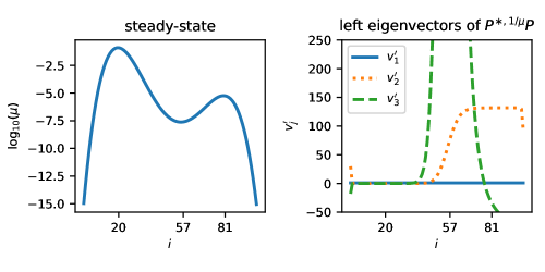
Figure 1. Left: the steady-state $\mu$. Right: the eigenvectors of $P^{\ast,1/\mu}P$. Note that $v^{\prime}_{1}$ and $v^{\prime}_{2}$ are approximately constant on the basins of attraction of the local minima of $V$, which correspond to maxima of the steady-state distribution. Here, the local minima of $\mu$ at $i=57$ and $i=0$ separate the basins of attraction. Note that $i=0$ and $i=100$ are identified, since we impose periodic boundary conditions.

We compute $\rho(J(\mu))$ and the upper bounds in Theorem 2 for several different choices of coarse states. First, we test uniform grids. We show for this simple, one-dimensional system that IAD converges quickly whenever the coarse states are sufficiently refined. Therefore, one does not need detailed prior knowledge of the eigenvectors of $P$ to choose good coarse states for this problem. For any $n\in\mathbb{N}$ and $\ell\in\{0,\dots,\lfloor 100/n\rfloor\}$, we define the uniform grid of coarse states

$$S_{J}=\left\{\left\lfloor J\frac{100}{n}\right\rfloor+\ell,\dots,+\left\lfloor(J+1)\frac{100}{n}\right\rfloor+\ell-1\right\}$$ (24)

for $J=0,\dots,n-2$, and

$$S_{n}=\{0,\dots,\ell-1\}\cup\left\{\left\lfloor(n-1)\frac{100}{n}\right\rfloor,\dots,99\right\}.$$

For example, for $n=2$ and $\ell=5$, the coarse states would be $S_{0}=\{5,\dots,54\}$ and $S_{1}=\{0,\dots,4\}\cup\{55,\dots,99\}$. In Figure 2, we report the maximum of $\rho(J(\mu))$ over all $l=0,\dots,\lfloor 100/n\rfloor$ for $n=1,\dots,20$. We see a clear decreasing trend with a growing number of coarse states.

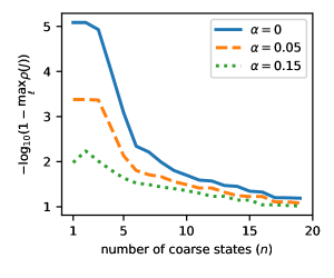
Figure 2. The maximum of $\rho(J(\mu))$ over all $l=0,\dots,\lfloor 100/n\rfloor$ for $n=1,\dots,20$ for the uniform grids of coarse states defined in (24). The curve labeled $\alpha=0$ is for the reversible chain of Section 6.3. The other curves are for the irreversible chains in Section 6.4.

We now investigate the dependence of $\rho(J(\mu))$ on the choice of coarse states in more detail. We compute the spectral radius $\rho(J(\mu))$ and our upper bounds for a family of coarse states of the form

$$S_{1}=\{0,...,\ell\}\text{ and }S_{2}=\{\ell+1,...,99\},$$ (25)

with $\ell=0,\dots,98$. We display the results in Figure 3. Different locations $\ell$ of the boundary between coarse states result in different angles $\theta$, depending on how well $v^{\prime}_{2}$ can be approximated by vectors that are constant on the coarse states. We expect $\theta$ to be small when the boundary between the coarse states coincides with the boundary between the basins of attraction, and this happens when $\ell=57$. Note that when $\ell$ is close to $57$, $\rho(J(\mu))\approx\sqrt{\lambda_{3}}$, and it is as if one has eliminated the larger eigenvalue $\sqrt{\lambda_{2}}$. When $\ell$ is far from $57$, $\rho(J(\mu))\approx\sqrt{\lambda_{2}}$, and IAD will converge at approximately the same rate as the power method. Note that both of the upper bounds in Theorem 3 yield precise estimates of $\rho(J(\mu))$, but the norm bound (15) is so precise as to be indistinguishable from the spectral radius $\rho(J(\mu))$.

Note that the optimal coarse states in the family (25) considered above coincide with the basins of attraction of $V$. We wish to emphasize that it is not in general necessary to choose the coarse states to be the basins of attraction. It is only necessary that the leading left eigenvectors of $P$ be well-approximated by functions that are constant on the coarse states. Note that this will be true whenever the coarse states are sufficiently refined.

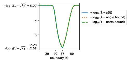
Figure 3. The spectral radius $\rho(J(\mu))$, the norm upper bound (15), and the angle upper bound (16) for the reversible, one-dimensional chain. Each of these numbers $x$ is very close to one for all values of $\ell$, so we plot $-\log_{10}(1-x)$. The variable $\ell$ on the horizontal axis relates to the definition of the coarse states, cf. equation (25). The spectral radius and the norm bound are indistinguishable in this figure.

6.4. IAD for Irreversible Chains on a One-Dimensional Grid

We now consider irreversible perturbations of the last process. Define

$$P_{\alpha}=(1-\alpha)P+\alpha W,$$

where $P$ is as above, $W$ is the right shift matrix (23), and $\alpha\in[0,1]$. Let $\mu_{\alpha}$ be the steady-state of $P_{\alpha}$. We compute $\rho(J(\mu_{\alpha}))$ and the upper bounds for the families of coarse states defined above in Section 6.3. We will see that our bounds are not as precise for irreversible chains as reversible chains. For $\alpha=0.05$, our bounds overestimate the true rate of convergence, but correctly predict the dependence of the rate on the choice of coarse states. For $\alpha=0.15$, our bounds do not seem to yield any useful information about the dependence of the rate of convergence on the coarse states. However, we note that $P_{0.15}$ is not metastable: we have $\rho(\hat{P}_{0.15})\approx 0.99$ compared with $\rho(\hat{P})\approx 0.99999$, cf. Table 2. Therefore, one does not need a sophisticated method like IAD to estimate the steady-state of a kernel like $P_{0.15}$, so $P_{0.15}$ is not of much interest as a test case for IAD. We include results for $\alpha=0.15$ simply to illustrate the limitations of our theory.

In Figure 2, we report the maximum of $\rho(J(\mu_{\alpha}))$ over all $l=0,\dots,\lfloor 100/n\rfloor$ for $n=1,\dots,20$. We see a clear decreasing trend with a growing number of coarse states. However, note that the spectral radius does not decrease monotonically with the number of coarse states for $\alpha=0.15$. In particular, for some choices of coarse states with $n=2$, $\rho(J(\mu_{0.15}))$ is larger than $\rho(\hat{P}_{0.15})$. For such poor choices of coarse states, IAD would converge more slowly than the power method.

In Figure 5, we report $\rho(J(\mu_{\alpha}))$ and the upper bounds for the family of shifted coarse states (25) for $\alpha=0.05$. We report the steady-state $\mu_{\alpha}$ and the three leading left eigenvectors of $P_{\alpha}$ in Figure 5. Note the similarity with the eigenvectors of $P_{0}$ in Figure 1. Our upper bounds correctly predict the dependence of $\rho(J(\mu_{\alpha}))$ on $\ell$. However, note that when $\ell$ is far from the optimal value, $\rho(J(\mu_{\alpha}))$ is almost the same as $\rho(\hat{P}_{\alpha})$, which is the asymptotic rate of convergence of the power method. Our estimates in Theorem 3 predict the slower rate of convergence $\sqrt{\lambda_{2}}$, which is the contraction constant of the power method in $\ell^{2}(1/\mu)$. Recall that all of our upper bounds on $\rho(J(\mu))$ are in fact upper bounds on $\lVert(I-\Pi(\mu))J(\mu)\rVert_{1/\mu}$. Note that although our bounds are generally quite close to $\lVert(I-\Pi(\mu))J(\mu)\rVert_{1/\mu}$, they sometimes significantly overestimate $\rho(J(\mu))$, cf. the discussion after the statement of Theorem 3.

In Figure 6, we report $\rho(J(\mu_{\alpha}))$ and the upper bounds for the family of shifted coarse states (25) for $\alpha=0.15$. Here, our upper bounds do not seem to yield any useful information about the dependence of the convergence rate on the choice of coarse states. We propose that more precise estimates based on the exact formula for the spectral radius given in Theorem 4 could be developed to understand the rate of convergence in this case. We leave this for future work. Note also that for some values of $\ell$, we have $\rho(J(\mu_{\alpha}))>\rho(\hat{P}_{\alpha})$, which indicates that IAD would converge more slowly than the power method.

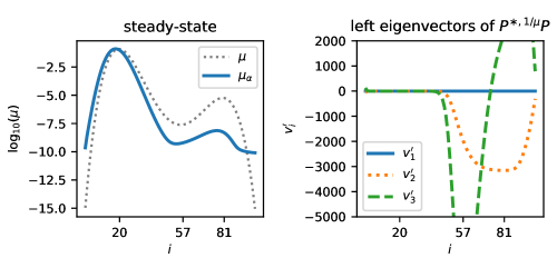
Figure 4. Left: The steady-state distribution $\mu_{\alpha}$ of $P_{\alpha}$ for $\alpha=0.05$. For comparison, we have included the discrete Boltzmann distribution $\mu$ as well. Right: The first three left eigenvectors of $P^{\ast,1/{\mu_{\alpha}}}_{\alpha}P_{\alpha}$ for $\alpha=0.05$.

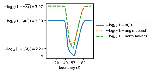
Figure 5. The spectral radius $\rho(J(\mu_{\alpha}))$, the norm upper bound (15), and the angle upper bound (16) with $k=2$ for the irreversible, one-dimensional chain $P_{\alpha}$ with $\alpha=0.05$. Each of these numbers $x$ is very close to one for all values of $\ell$, so we report $-\log_{10}(1-x)$. The variable $\ell$ on the horizontal axis relates to the definition of the coarse states, cf. (25).

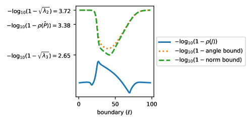
Figure 6. The spectral radius $\rho(J(\mu_{\alpha}))$, the norm upper bound (15), and the angle upper bound (16) with $k=2$ for the irreversible, one-dimensional chain $P_{\alpha}$ with $\alpha=0.15$. Each of these numbers $x$ is very close to one for all values of $\ell$, so we report $-\log_{10}(1-x)$. The variable $\ell$ on the horizontal axis relates to the definition of the coarse states, cf. (25).

Table 2. The spectral radius $\rho(\hat{P}_{\alpha})$ for $\alpha=0,0.05,0.15$. Note that for $\alpha=0$, $P_{\alpha}$ is simply the reversible chain defined in Section 6.3. Observe that for $\alpha=0.15$, the chain converges very quickly compared with $\alpha=0$.

$\alpha$	$\rho(\hat{P}_{\alpha})$	$-\log_{10}(1-\rho(\hat{P}_{\alpha}))$
$0$	$0.999992$	$5.09$
$0.05$	$0.999581$	$3.38$
$0.15$	$0.989564$	$1.98$

6.5. IAD for a Metastable Chain on a Two-Dimensional Grid

We now consider a metastable chain on a two-dimensional grid. Molecular models and other models in computational chemistry usually involve stochastic processes on spaces having thousands or millions of dimensions. Of course, when the dimension is so high, one cannot expect to cover space by a uniform grid of coarse states. Therefore, in many sampling strategies, one chooses a low-dimensional coordinate to discretize. We demonstrate for a model two-dimensional system that one can attain a significant reduction in the rate of convergence by discretizing a single variable into a small number of coarse states.

Define $V:\mathbb{R}^{2}\rightarrow\mathbb{R}$ by

$$\begin{split}V(x,y)&=3\exp\left(-x^{2}-\left(y-\frac{1}{3}\right)^{2}\right)-3\exp\left(-x^{2}-\left(y^{2}-\frac{5}{3}\right)^{2}\right)\\ &\qquad-5\exp\left(-\left(x-1\right)^{2}-y^{2}\right)-5\exp\left(-\left(x+1\right)^{2}-y^{2}\right).\end{split}$$

See Figure 7. This simple potential function was proposed for a study of reaction rates in [27]. Let $\mu$ be the discrete Boltzmann distribution on a two-dimensional grid with $V$ as above and with $[a,b]\times[c,d]=[-1.7,1.7]\times[-1.7,2]$, $N=50$, and $T=1/4$. Let $P$ be the corresponding reversible Markov chain. The definitions of the discrete Boltzmann distribution and the reversible dynamics are analogous to the one-dimensional case. See Appendix F for details. We report the largest $5$ eigenvalues of $P$ in Table 3, and we display the left eigenvectors $v^{\prime}_{2}$ and $v^{\prime}_{3}$ in Figures 8 and 9.

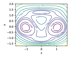
Figure 7. A Contour map of the potential function $V$. Note the two global minima on the left and right and the local minimum along a path betweeen the other two at the top.

Define the coarse states

$$S_{I}=\left\{(i,j)\in\{1,\dots,N\}^{2}:\left\lfloor\frac{i}{3}\right\rfloor=j\right\}\text{ for }I=0,1,2.$$ (26)

Here, $P$ is a Markov chain on the state space $\{1,\dots,50\}\times\{1,\dots,50\}$, and the coarse states discretize only the first variable, not the second. The outlines of the coarse states are visible in the left panel of Figure 8. We report $\rho(J(\mu))$, the norm upper bound (15), and the angle upper bound (16) for $k=2$ and $k=3$ for this choice of coarse states in Table 4. Note that $\sin^{2}(\theta)\approx 0.002$ is quite small. We display the eigenvector $v^{\prime}_{2}$ and its best approximation in the $\ell^{2}(\mu)$-norm in Figure 8. Although the two vectors may not appear to be aligned, they are in fact very close in the $\ell^{2}(\mu)$-norm since the regions where they differ have very small probability under $\mu$ and the maximum size of the difference between the vectors is not large in comparison to the very small probability. Observe that in this case, even with very few coarse states that discretize only a single dimension, we have in effect eliminated the largest eigenvalue $\sqrt{\lambda_{2}}$, and the rate of convergence of IAD is essentially equal to $\sqrt{\lambda_{3}}$. Note that $\sin^{2}(\theta)$ is large for $k=3$ in this case, so $v^{\prime}_{3}$ is not well-approximated by a vector that is constant on the coarse states, cf. Figure 9.

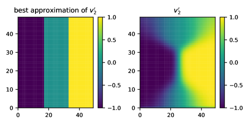
Figure 8. Right: The second left eigenvector $v^{\prime}_{2}$ of $P^{\ast,1/\mu}P$. Left: The best approximation $\Pi(\mu)^{\mathrm{t}}v^{\prime}_{2}$ of $v^{\prime}_{2}$ in the $\ell^{2}(\mu)$-norm by a function that is constant on the one-dimensional grid of coarse states (26). Note that this figure could also be interpreted as a depiction of the coarse states themselves.

Table 3. The largest five eigenvalues of $P^{\ast,1/\mu}P$ for the reversible, two-dimensional chain $P$ of Section 6.5. We report $\sqrt{\lambda_{k}}$ instead of $\lambda_{k}$, since it is $\sqrt{\lambda_{k}}$ that appears in Theorem 3.

$k$	$\sqrt{\lambda_{k}}$
$1$	$1$
$2$	$0.999997$
$3$	$0.999488$
$4$	$0.997511$
$5$	$0.994219$

Table 4. The spectral radius $\rho(J(\mu))$, the norm upper bound (15), and the angle upper bound (16) together with $\sin^{2}(\theta)$ for $k=2,3$. The first column is for the one-dimensional grid (26) and the second column is for the six-by-six, two-dimensional grid (27)

	1-d Grid	2-d Grid
$\rho(J(\mu))$	$0.999410$	$0.987327$
norm bound	$0.999410$	$0.987327$
$\sin^{2}(\theta)$, $k=2$	$0.002382$	$0.000143$
angle bound, $k=2$	$0.999650$	$0.999502$
$\sin^{2}(\theta)$, $k=3$	$0.854170$	$0.031745$
angle bound, $k=3$	$0.999997$	$0.999920$

We now test a six-by-six, two-dimensional grid of coarse states that refines the one-dimensional grid of three coarse states used above. For all $I,J\in\{0,\dots,5\}$, we let

$$S_{IJ}=\left\{(x,y)\in\{1,\dots,N\}^{2}:\left\lfloor\frac{x}{6}\right\rfloor=I\text{ and }\left\lfloor\frac{y}{6}\right\rfloor=J\right\}.$$ (27)

One can see the outlines of some of these coarse states in the left panel of Figure 9. We report $\rho(J(\mu))$ and the upper bounds for this choice of coarse states in Table 4. Note that both the spectral radius and the upper bounds are smaller, as expected for a refinement of the coarse states given the discussion following Corollary 1. For our six-by-six grid, $\sin^{2}(\theta)$ for $k=3$ is much smaller than for the one-dimensional grid. However, it is not small enough that the angle upper bound for $k=3$ is actually lower than for $k=2$. In fact, the interpolation between $\sqrt{\lambda_{k+1}}$ and $\sqrt{\lambda_{2}}$ in (16) is very steep, and one needs a very small value of $\sin^{2}(\theta)$ for the upper bound to approximate $\sqrt{\lambda_{k+1}}$. Nonetheless, refining the set of coarse states reduces $\rho(J(\mu))$ significantly, and this is correctly predicted by the norm upper bound (15).

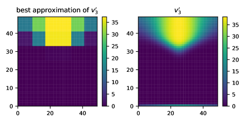
Figure 9. Right: The third left eigenvector $v^{\prime}_{3}$ of $P^{\ast,1/\mu}P$. Left: The best approximation $\Pi(\mu)^{\mathrm{t}}v^{\prime}_{3}$ of $v^{\prime}_{3}$ in the $\ell^{2}(\mu)$-norm by a function that is constant on the two-dimensional grid of coarse states (26).

7. Conclusion

Our work here was motivated by a desire to understand the robustness and efficiency of methods such as nonequilibrium umbrella sampling (NEUS) [35], exact milestoning [1], and injection measures [10] for calculating nonequilibrium (or equilibrium) steady-states in statistical physics. We have studied IAD as a simple model of this class of methods. We explain why it may be possible to use methods similar to IAD to efficiently compute steady-states of molecular models and how one might choose the coarse states in practice to optimize efficiency. For reversible processes, we conclude that one should choose coarse states so that the leading left eigenvectors of $P$ are well-approximated in the $\ell^{2}(\mu)$-norm by vectors that are constant on the coarse states. Since error is measured in the $\ell^{2}(\mu)$-norm, regions of low probability will not have a significant influence on the approximation quality unless some of the leading eigenvectors are concentrated in those regions. This means that in some cases a very naïve choice of coarse states can be efficient. For irreversible processes, our conclusions are similar but not so definite. For some very irreversible processes, our upper bounds do not yield much information about the dependence of the asymptotic rate of convergence on the choice of strata. Although our primary interests lie in statistical physics, our results are general, and we hope others will apply them to understand the performance of IAD in other contexts.

Our work does not address all important points. We show only local convergence, not global. We focus primarily on estimates of the asymptotic rate of convergence, ignoring preasymptotic phenomena. We recall that NEUS and similar methods are stochastic evolving particle systems that approximate IAD; we do not consider issues related to the particle approximation. We leave these points for future work.

Appendix A Computing the Coarse Steady-State

We compute the coarse steady-state $z(C(\mu^{k}))$ by the following algorithm.

Algorithm 2.

Assume that $C(\mu^{k})$ is irreducible as guaranteed by Lemma 1. The user must specify an error tolerance $\tau>0$ and an exponent $k\in\mathbb{N}$. In our numerical experiments in Sections 6.3 and 6.5, we take $\tau=10^{-9}$ and $k=2^{15}$. We compute $z(C(\mu^{k}))$ by the following procedure:

1. Set $\bar{C}=\frac{1}{2}(I+C(\mu^{k}))$. Use the algorithm in [12] to compute an initial approximation $\tilde{z}$ to the steady-state $z(C(\mu^{k}))$ from the $QR$-factorization of $I-\bar{C}$.

2. Refine the initial approximation $\bar{z}$ using a power method:

   1. Set $z^{\text{old}}=\bar{z}$.

   2. Calculate

      $$z^{\text{new}}=\bar{C}^{k}z^{\text{old}}.$$

   3. If

      $$\max_{i=1,\dots,n}\frac{\lvert z^{\text{new}}_{i}-Cz^{\text{new}}_{i}\rvert}{z^{\text{new}}_{i}}<\tau\text{ and }\frac{\lvert z^{\text{new}}_{i}-z^{\text{old}}_{i}\rvert}{z^{\text{old}}_{i}}<\tau$$

      then return $z^{\text{new}}$ to the user. Otherwise, set $z^{\text{old}}=z^{\text{new}}$ and go to step (b) above.

In practice, we find that direct methods (like the algorithm in [12]) for calculating the coarse-steady state are often not sufficiently accurate. When direct methods produce an inaccurate result, applying a few power method iterations has usually produced a much better estimate of the steady-state.

Appendix B Well-posedness of IAD

Here, we prove that IAD is well-posed under our assumptions, and we give some examples to illustrate what can go wrong when our assumptions do not hold.

B.1. Proof of Lemma 1

We show that IAD is well-posed if $P$ is irreducible and $\mu^{0}>0$.

Proof.

First, we show that if $P$ is irreducible and $\nu>0$, then $C(\nu)$ is irreducible. We prove the contrapositive, showing that if $\nu>0$ and $C(\nu)$ is reducible, then $P$ is reducible. If $\nu>0$ and $C(\nu)$ is reducible, then there is a partition of the coarse states

$$\{1,\dots,n\}=A\cup B$$

into disjoint and nonempty sets $A$ and $B$ so that for all $a\in A$ and $b\in B$

$$C(\nu)_{ab}=APD(\nu)_{ab}=\sum_{\begin{subarray}{c}i\in S_{a}\\ j\in S_{b}\end{subarray}}\frac{\nu_{i}}{A\nu_{a}}P_{ji}=0.$$

Therefore, since $\nu>0$, $P_{ji}=0$ for all $i\in S_{a}$ and $j\in S_{b}$. Now define

$$\mathcal{A}=\cup_{a\in A}S_{a}\text{ and }\mathcal{B}=\cup_{b\in B}S_{b}.$$

The sets $\mathcal{A}$ and $\mathcal{B}$ are a partition of $\Omega$ into disjoint and nonempty sets, and we have $P_{ji}=0$ for any $i\in\mathcal{A}$ and $j\in\mathcal{B}$. It follows that $P$ must be reducible. We conclude that if $\nu>0$ and $P$ is irreducible, then $C(\nu)$ must be irreducible.

Now we show that if $\mu^{k}>0$, then $\mu^{k+1}>0$. To verify that $\mu^{k+\frac{1}{2}}>0$, we observe that $C(\mu^{k})$ is irreducible when $\mu^{k}>0$ by the previous paragraph, and so the steady-state $z(C(\mu^{k}))$ is unique and positive by the Perron–Frobenius theorem. It follows that $\mu^{k+\frac{1}{2}}=D(\mu^{k})z(C(\mu_{k}))>0$. Moreover, when $P$ is irreducible, $\nu>0$ implies $P\nu>0$. To see this, observe that if $\nu>0$, then for any $i\in\Omega$ with $P\nu_{i}=0$, $P_{ij}=0$ for all $j\neq i$. Thus, $P$ is reducible if $P\nu$ is not positive. Therefore, $\mu^{k+1}=P\mu^{k+\frac{1}{2}}>0$ if $\mu^{k}>0$, and by induction $\mu^{0}>0$ implies $\mu^{k}>0$ for all $k\in\mathbb{N}$. This concludes the proof that the iterates $\mu^{k}$ are well-defined. ∎

B.2. Examples motivating our assumptions

We now give some pathological examples to motivate our assumptions that $\mu^{0}>0$ and that $P^{\mathrm{t}}P$ is irreducible.

B.2.1. Positive initial condition ($\mu^{0}>0$)

We assume $\mu^{0}>0$, since if $\mu^{0}$ is not positive, then $C(\mu^{0})$ may be reducible even when $P$ and $P^{\mathrm{t}}P$ are irreducible and aperiodic. For example, consider the chain on $\Omega=\{1,2,3\}$ with transition matrix

$$P=\begin{pmatrix}0&\frac{1}{3}&0\\ 1&\frac{1}{3}&1\\ 0&\frac{1}{3}&0\end{pmatrix}.$$

Here, $P$ and $P^{\mathrm{t}}P$ are irreducible and aperiodic. Now define the coarse states

$$S_{1}=\{1,2\}\text{ and }S_{2}=\{3\}.$$

For $\mu^{0}=\frac{1}{2}(\delta_{1}+\delta_{3})=(\frac{1}{2},0,\frac{1}{2})^{\mathrm{t}}$, we have

$$C(\mu^{0})=APD(\mu^{0})=\begin{pmatrix}1&1\\ 0&0\\ \end{pmatrix},$$

which is reducible.

B.2.2. $P^{\mathrm{t}}P$ irreducible

We assume that $P^{\mathrm{t}}P$ is irreducible to prove local convergence of IAD. It was observed in [23, Example 2] that IAD is not locally convergent for

$$P=\begin{pmatrix}0&1&0&\frac{1}{2}\\ \frac{1}{2}&0&0&0\\ \frac{1}{2}&0&0&\frac{1}{2}\\ 0&0&1&0\end{pmatrix}$$

with the strata $S_{1}=\{1,2\}$ and $S_{2}=\{3,4\}$. However, $P$ is irreducible and aperiodic, so the Markov chain with transition matrix $P$ is convergent. The reader will note that $P^{\mathrm{t}}P$ is reducible, so this is an example where the power method is convergent but not a strict contraction in $\ell^{2}(1/\mu)$.

Appendix C Proofs of results stated in Section 4.1

C.1. Proof of Lemma 2

We begin with a proof of Lemma 2, which shows that the time reversal of $P$ is its adjoint $P^{\ast,1/\mu}$.

Proof of Lemma 2.

For simplicity, we write $\langle,\rangle$ for $\langle,\rangle_{1/\mu}$ and $P^{\ast}$ for $P^{\ast,1/\mu}$. Note that for any $x,y\in\mathbb{R}^{N}$, we have

$$\langle x,Py\rangle =\langle x,\operatorname{diag}(1/\mu)Py\rangle_{\mathds{1}}$$

$$=\langle\operatorname{diag}(\mu)P^{\mathrm{t}}\operatorname{diag}(1/\mu)x,\operatorname{diag}(1/\mu)y\rangle_{\mathds{1}}$$

$$=\langle\operatorname{diag}(\mu)P^{\mathrm{t}}\operatorname{diag}(1/\mu)x,y\rangle,$$

so

$$P^{\ast}=\operatorname{diag}(\mu)P^{\mathrm{t}}\operatorname{diag}(1/\mu).$$ (28)

Therefore, $P^{\ast}_{ij}=\frac{P_{ji}\mu^{j}}{\mu_{i}}$, which is exactly the time-reversal of $P$. See [26, Theorem 1.9.1] for the definition of the time-reversal and its properties. (Remember that $P$ is column stochastic, so the time reversal here takes a slightly different form than for the row stochastic matrices of [26].) The time-reversal $P^{\ast}$ is column stochastic and has the same invariant distribution $\mu$ as $P$, since time-reversals always have these properties. ∎

C.2. Proof of Lemma 3

We now prove convergence of the power method when both $P$ and $P^{\mathrm{t}}P$ are irreducible. The condition $P^{\mathrm{t}}P$ implies that the stochastic matrix $P^{\ast,1/\mu}P$ is irreducible, and this is the essential fact in our proof that the power method is strictly contracting in the $\ell^{2}(1/\mu)$-norm.

Proof of Lemma 3.

To simplify notation, for any $M\in\mathbb{R}^{N\times N}$, we write $M^{\ast}$ for $M^{\ast,1/\mu}$ and $M^{\mathrm{t}}$ for the transpose. We let $\lVert\cdot\rVert$ and $\langle,\rangle$ denote the $\ell^{2}(1/\mu)$-norm and inner product. Since $P$ is column stochastic and $\nu^{0}$ is a probability vector, $\nu^{k}$ is a probability vector for all $k\in\mathbb{N}$, so $\mathds{1}^{\mathrm{t}}\nu^{k}=1$. Therefore,

$$\nu^{k+1}-\mu =P\nu^{k}-\mu$$

$$=(P-\mu\mathds{1}^{\mathrm{t}})\nu^{k}$$

$$=(P-\mu\mathds{1}^{\mathrm{t}})(\nu^{k}-\mu)$$

$$=\hat{P}(\nu^{k}-\mu).$$

Note that the third equality above follows since $P\mu=\mu$ and $\mu$ is a probability vector.

We now observe that for any $M\in\mathbb{R}^{N\times N}$, we have

$$\lVert M\rVert=\rho(M^{\ast}M)^{\frac{1}{2}}=\lVert M^{\ast}M\rVert^{\frac{1}{2}}.$$ (29)

In particular, $\lVert\hat{P}\rVert=\rho(\hat{P}^{\ast}\hat{P})^{\frac{1}{2}}=\lVert\hat{P}^{\ast}\hat{P}\rVert^{\frac{1}{2}}$. The analogous result

$$\lVert M\rVert_{\mathds{1}}=\rho(M^{\mathrm{t}}M)^{\frac{1}{2}}=\lVert M^{\mathrm{t}}M\rVert_{\mathds{1}}^{\frac{1}{2}}$$

for the uniformly weighted $\ell^{2}(\mathds{1})$-inner product is well-known, and the standard proof generalizes to any inner product space. Therefore, it will suffice to show that $\rho(\hat{P}^{\ast}\hat{P})^{\frac{1}{2}}<\sqrt{\lambda_{2}}$. Observe that

$$\hat{P}^{\ast}\hat{P} =(P^{\ast}-\mu\mathds{1}^{\mathrm{t}})(P-\mu\mathds{1}^{\mathrm{t}})$$

$$=P^{\ast}P-P^{\ast}\mu\mathds{1}^{\mathrm{t}}-\mu\mathds{1}^{\mathrm{t}}P+\mu\mathds{1}^{\mathrm{t}}$$

$$=P^{\ast}P-\mu\mathds{1}^{\mathrm{t}},$$

so $\rho(\hat{P}^{\ast}\hat{P})=\lambda_{2}$ by the diagonalization (4) of $P^{\ast}P$. Thus, $\lVert\hat{P}\rVert=\sqrt{\lambda_{2}}$.

By (28), $P^{\ast}P$ is irreducible if and only if $P^{\mathrm{t}}P$ is irreducible. Moreover, $\lVert\hat{P}\rVert=\sqrt{\lambda_{2}}<1$ if $P^{\ast}P$ is irreducible by the Perron–Frobenius theorem, cf.[25, Section 8.3, pg. 673]. Therefore, $P^{\mathrm{t}}P$ irreducible is a sufficient condition for $\lVert\hat{P}\rVert<1$. To see that it is also a necessary condition, we will prove that if $P^{\mathrm{t}}P$ is reducible, then $\lVert\hat{P}\rVert\geq 1$. If $P^{\mathrm{t}}P$ is reducible, then there exist nonempty, disjoint subsets $A$ and $B$ of $\Omega$ so that $P^{t}P_{ij}=0$ for all $i\in A$ and $j\in B$. Since $P^{\mathrm{t}}P$ is symmetric, we also have $P^{\mathrm{t}}P_{ij}=0$ for $i\in B$ and $j\in A$. Therefore, $P^{\ast}P$ admits a block decomposition of the form

$$P^{\ast}P=\bordermatrix{~{}&A&B\cr A&P_{1}&0\cr B&0&P_{2}},$$

where $P_{1}$ and $P_{2}$ are both column stochastic matrices. Let $v_{1}$ and $v_{2}$ be steady-state probability vectors of $P_{1}$ and $P_{2}$, respectively. Define $V_{1}=(v_{1},0)^{\mathrm{t}}$ and $V_{2}=(0,v_{2})^{\mathrm{t}}$. We have $V_{1}-V_{2}\neq 0$, and

$$\lVert\hat{P}(V_{1}-V_{2})\rVert^{2}=\lVert P(V_{1}-V_{2})\rVert^{2}=\langle P^{\ast}P(V_{1}-V_{2}),(V_{1}-V_{2})\rangle=\lVert V_{1}-V_{2}\rVert^{2},$$

which verifies $\lVert\hat{P}\rVert\geq 1$. ∎

Appendix D Proofs of results stated in Section 4.2

D.1. Proof of Lemma 4

We begin with a proof of Lemma 4, our reformulation of the steady-state eigenproblem $Qz(Q)=z(Q)$ as a linear system.

Proof of Lemma 4.

Observe that $x=z(Q)$ solves

$$(I-Q+vw^{\mathrm{t}})x=vw^{\mathrm{t}}z(Q),$$ (30)

since $Qz(Q)=z(Q)$. If we can show that $x=z(Q)$ is the unique solution of (30), then $I-Q+vw^{\mathrm{t}}$ is invertible and the result follows.

Suppose to the contrary that $u\neq z(Q)$ also solves (30). Then we have

$$\mathds{1}^{\mathrm{t}}(I-Q+vw^{\mathrm{t}})u=\mathds{1}^{\mathrm{t}}vw^{\mathrm{t}}u=\mathds{1}^{\mathrm{t}}vw^{\mathrm{t}}z(Q),$$

since $\mathds{1}^{\mathrm{t}}(I-Q)=0$ for any column stochastic $Q$. Therefore, $w^{\mathrm{t}}u=w^{\mathrm{t}}z(Q)$ since we assume $\mathds{1}^{\mathrm{t}}v\neq 0$. It follows, again by (30), that

$$(I-Q)u=0.$$

Moreover, since we assume $w^{\mathrm{t}}z(Q)\neq 0$, $u\neq z(Q)$ and $w^{\mathrm{t}}u=w^{\mathrm{t}}z(Q)$ imply

$$u\notin\operatorname{span}\{z(Q)\}.$$

Now recall that since $Q$ is irreducible, $z(Q)>0$ by the Perron–Frobenius theorem. Thus, for some $\varepsilon>0$, $z(Q)+\varepsilon u>0$, $z(Q)+\varepsilon u\notin\operatorname{span}\{z(Q)\}$, and

$$Q(z(Q)+\varepsilon u)=z(Q)+\varepsilon u.$$

This contradicts uniqueness of the stationary distribution of $Q$, so $z(Q)$ is the unique solution of (30), and $I-Q+vw^{\mathrm{t}}$ is invertible. ∎

D.2. Proof of Lemma 5

We prove our error propagation formula for the coarse correction step.

Proof of Lemma 5.

First, note that

$$A(I-P+\mu\mathds{1}^{\mathrm{t}})D(\nu)=I-C(\nu)+A\mu\mathds{1}^{\mathrm{t}}$$

is invertible by Lemma 4, since $C(\nu)$ is irreducible when $\nu>0$ by Lemma 1.

We prove formula (8) for the error after the coarse correction. Using our reformulations (6) and (7) of the steady-state problems, we have

$$\mu^{k+\frac{1}{2}} =D(\mu^{k})z(C(\mu^{k}))$$

$$=D(\mu^{k})(I-C(\mu^{k})+A\mu\mathds{1}^{\mathrm{t}})^{-1}A\mu$$

$$=D(\mu^{k})(A(I-P+\mu\mathds{1}^{\mathrm{t}})D(\mu^{k}))^{-1}A\mu$$

$$=D(\mu^{k})(A(I-P+\mu\mathds{1}^{\mathrm{t}})D(\mu^{k}))^{-1}A(I-P+\mu\mathds{1}^{\mathrm{t}})\mu$$

$$=S(\mu^{k})\mu.$$

Now since $D(\mu^{k})\mu^{k}=\mu^{k}$, we have

$$S(\mu^{k})\mu^{k} =D(\mu^{k})(A(I-P+\mu\mathds{1}^{\mathrm{t}})D(\mu^{k}))^{-1}A(I-P+\mu\mathds{1}^{\mathrm{t}})\mu^{k}$$

$$=D(\mu^{k})(A(I-P+\mu\mathds{1}^{\mathrm{t}})D(\mu^{k}))^{-1}A(I-P+\mu\mathds{1}^{\mathrm{t}})D(\mu^{k})\mu^{k}$$

$$=\mu^{k}.$$

Therefore,

$$\mu^{k+\frac{1}{2}}-\mu=(I-S(\mu^{k}))\mu=(I-S(\mu^{k}))(\mu^{k}-\mu),$$

as desired.

It remains to show that $S(\nu)$ is a projection on $\operatorname{Rg}(D(\nu))$. For convenience, we write $S$ for $S(\nu)$, $D$ for $D(\nu)$, and $C$ for $C(\nu)$. To see that $S$ is a projection, observe that

$$S^{2} =D[A(I-\hat{P})D]^{-1}(A(I-\hat{P})D)[A(I-\hat{P})D]^{-1}A(I-\hat{P})$$

$$=D[A(I-\hat{P})D]^{-1}A(I-\hat{P})$$

$$=S.$$

To see that $\operatorname{Rg}(S)=\operatorname{Rg}(D)$, first observe that

$$\operatorname{Rg}(A(I-\hat{P}))=\operatorname{Rg}(A)=\mathbb{R}^{n},$$

since $(I-\hat{P})$ is invertible by Lemma 4. Therefore, since $A(I-\hat{P})D=I-C+A\mu\mathds{1}^{\mathrm{t}}$ is also invertible by Lemma 4,

$$\operatorname{Rg}([A(I-\hat{P})D]^{-1}A(I-\hat{P}))=\mathbb{R}^{n},$$

and it follows that $\operatorname{Rg}(S)=\operatorname{Rg}(D)$. ∎

D.3. IAD as an Algebraic Multigrid Method

Here, we explain that IAD is more-or-less an adaptive algebraic multigrid method. Roughly similar observations appear in [15]. Recall that the steady-state $\mu$ is the unique solution $x$ of the linear system of equations

$$(I-P+\mu\mathds{1}^{\mathrm{t}})x=\mu,$$

cf. (6). Suppose that one were to try to solve this equation by algebraic multigrid with the restriction operator $A$. Typically, the prolongation operator would be the transpose of restriction. Suppose that instead one were to take an adjoint with respect to some non-uniform inner product. For example, let $\nu\in\mathbb{R}^{N}$ be a positive probability vector, and define the prolongation operator to be the operator $A^{\dagger}\in\mathbb{R}^{N\times n}$ satisfying

$$\langle A\eta,w\rangle_{1/A\nu}=\langle\eta,A^{\dagger}w\rangle_{1/\nu}$$

for all $w\in\mathbb{R}^{n}$ and $\eta\in\mathbb{R}^{N}$. By Lemma 11, we have $A^{\dagger}=D(\nu)$.

The coarse grid correction step for a multigrid method with restriction operator $A$ and prolongation $D(\nu)$ is

$$\mu^{k+\frac{1}{2}} =\mu^{k}+D(\nu)(A(I-P+\mu\mathds{1}^{\mathrm{t}})D(\nu))^{-1}A(\mu-(I-P+\mu\mathds{1}^{\mathrm{t}})\mu^{k})$$

$$=\mu^{k}+D(\nu)(A(I-P+\mu\mathds{1}^{\mathrm{t}})D(\nu))^{-1}A(I-P+\mu\mathds{1}^{\mathrm{t}})(\mu-\mu^{k})$$

$$=\mu^{k}-S(\nu)(\mu^{k}-\mu),$$

where $S(\nu)$ is the coarse projection defined in Lemma 5. Here, the residual is $\mu-(I-P+\mu\mathds{1}^{\mathrm{t}})\mu^{k}$ and the coarse system matrix is $A(I-P+\mu\mathds{1}^{\mathrm{t}})D(\nu)$. Note that if one chooses $\nu=\mu^{k}$, the coarse grid correction is equivalent with the coarse correction step of IAD. After the coarse grid correction in a multigrid method, one computes several steps of a smoothing iteration, often using some version of the Jacobi or Gauss-Seidel method. In IAD, one performs a step of the power method, which corresponds to using $P$ as the smoothing matrix.

Note that IAD is not a true multigrid method since the inner product and therefore the prolongation operator depend on the current approximation $\mu^{k}$ of $\mu$. Thus, IAD is nonlinear and the standard theory of multigrid methods does not apply.

D.4. Proof of Lemma 7

We prove that $\Pi(\nu)$ is an $\ell^{2}(\nu)$-orthogonal projection. We begin by showing that $A$ and $D(\nu)$ are adjoint in a certain sense.

Lemma 11.

For any $w\in\mathbb{R}^{n}$ and $\eta\in\mathbb{R}^{N}$, we have

$$\langle D(\nu)w,\eta\rangle_{1/\nu}=\langle w,A\eta\rangle_{1/A\nu}.$$

Proof.

We have

$$\langle D(\nu)w,\eta\rangle_{1/\nu} =\sum_{j=1}^{N}\sum_{k=1}^{n}w_{k}\nu(j|S_{k})\eta_{j}\frac{1}{\nu_{j}}$$

$$=\sum_{j=1}^{N}\sum_{k=1}^{n}w_{k}\frac{\mathds{1}_{S_{k}}(j)}{A\nu_{k}}\eta j$$

$$=\sum_{k=1}^{n}w_{k}\left(\sum_{j=1}^{N}\mathds{1}_{S_{k}}(j)\eta_{j}\right)\frac{1}{A\nu_{k}}$$

$$=\langle w,A\eta\rangle_{1/A\nu}.$$

∎

We now prove Lemma 7, which verifies that $\Pi(\nu)$ is an orthgonal projection.

Proof of Lemma 7.

First, note that

$$AD(\nu)=I\in\mathbb{R}^{N\times N}.$$

Therefore,

$$\Pi(\nu)^{2}=D(\nu)(AD(\nu))A=D(\nu)A=\Pi(\nu),$$

so $\Pi(\nu)$ is a projection.

To see that $\Pi(\nu)$ is orthogonal, note that by Lemma 11, for any $\eta,\kappa\in\mathbb{R}^{N}$,

$$\langle\Pi(\nu)\eta,\kappa\rangle_{1/\nu} =\langle D(\nu)A\eta,\kappa\rangle_{1/\nu}$$

$$=\langle A\eta,A\kappa\rangle_{1/A\nu}$$

$$=\langle\eta,D(\nu)A\kappa\rangle_{1/\nu}$$

$$=\langle\eta,\Pi(\nu)\kappa\rangle_{1/\nu}.$$

Therefore, $\Pi(\nu)^{\ast,1/\nu}=\Pi(\nu)$ so $\Pi(\nu)$ is an orthogonal projection in $\ell^{2}(1/\nu)$.

Finally, observe that $\Pi(\nu)=D(\nu)A$ is column stochastic, since both $A$ and $D(\nu)$ map probability vectors to probability vectors. We have $\Pi(\nu)\nu=\nu$ directly from the definition of $\Pi(\nu)$, and $\Pi(\nu)$ is reversible since it is self-adjoint with respect to the $\ell^{2}(1/\nu)$-inner product, cf. Lemma 2. ∎

D.5. Proof of Lemma 8

We begin our proof of Lemma 8 by computing the block decomposition of $J(\mu)$ with respect to $\Pi(\mu)$. The essential facts are summarized in the following simple lemma.

Lemma 12.

We have

$$\Pi(\mu)S(\mu)=S(\mu)\text{ and }S(\mu)\Pi(\mu)=\Pi(\mu).$$

Proof.

For convenience, we write $\Pi$ for $\Pi(\mu)$ and $S$ for $S(\mu)$. Since $S$ is a projection with $\operatorname{Rg}(S)=\operatorname{Rg}(\Pi)$ by Lemma 5, we have

$$S\Pi=\Pi.$$

Similarly, $\Pi S=S$. ∎

As a consequence of Lemma 12, we have the following block decomposition of $J(\mu)$.

Lemma 13.

We have

$$J(\mu)\Pi(\mu)=0,$$

and

$$\Pi(\mu)J(\mu)=\Pi(\mu)-S(\mu).$$

Proof.

For convenience, we write $J$ for $J(\mu)$, $\Pi$ for $\Pi(\mu)$, and $S$ for $S(\mu)$. By Lemma 12, $S\Pi=\Pi$, so

$$J\Pi=\hat{P}(I-S)\Pi=0.$$ (31)

We also have

$$\Pi J =\Pi\hat{P}(I-S)$$

$$=\Pi\hat{P}-\Pi\hat{P}S$$

$$=\Pi\hat{P}-D[A\hat{P}D(I-A\hat{P}D)^{-1}]A(I-\hat{P})$$

$$=\Pi\hat{P}-D[(I-A\hat{P}D)^{-1}-I]A(I-\hat{P})$$

$$=\Pi\hat{P}-D[(A(I-\hat{P})D)^{-1}-I]A(I-\hat{P})$$

$$=\Pi\hat{P}-S+\Pi(I-\hat{P})$$

$$=\Pi-S.$$

The fifth inequality above follows since $AD=I\in\mathbb{R}^{n\times n}$. ∎

By Lemma 13,

$$J(\mu)=J(\mu)(I-\Pi(\mu)).$$ (32)

This will be important in several of our proofs. It implies, for example, that

$$\sigma(J(\mu))=\sigma(J(\mu)(I-\Pi(\mu))=\sigma((I-\Pi(\mu))J(\mu)),$$ (33)

since $\sigma(AB)=\sigma(BA)$ for any matrices $A,B\in\mathbb{R}^{N\times N}$. We now proceed with the proof of Lemma 8.

Proof of Lemma 8.

For convenience, we write $J$ for $J(\mu)$, $\Pi$ for $\Pi(\mu)$, and $S$ for $S(\mu)$. For $x\in\mathbb{R}^{N}$,

$$\lVert Jx\rVert_{\varepsilon}^{2} =\lVert J(I-\Pi)x\rVert_{\varepsilon}^{2}$$

$$=\lVert(I-\Pi)J(I-\Pi)x\rVert_{1/\mu}^{2}+\varepsilon\lVert\Pi J(I-\Pi)x\rVert_{1/\mu}^{2}$$

$$\leq\left(\lVert(I-\Pi)J\rVert_{1/\mu}^{2}+\varepsilon\lVert\Pi J\rVert^{2}_{1/\mu}\right)\lVert(I-\Pi)x\rVert_{1/\mu}^{2}$$

$$\leq\left(\lVert(I-\Pi)J\rVert_{1/\mu}^{2}+\varepsilon\lVert\Pi J\rVert^{2}_{1/\mu}\right)\lVert x\rVert_{\varepsilon}^{2}$$

$$=\left(\lVert(I-\Pi)J\rVert_{1/\mu}^{2}+\varepsilon\lVert\Pi-S\rVert^{2}_{1/\mu}\right)\lVert x\rVert_{\varepsilon}^{2}$$

The first equality holds by (32). The inequality in the second to last step holds since $I-\Pi$ is an orthogonal projection and therefore $\lVert I-\Pi\rVert_{1/\mu}=1$. The last equality holds by Lemma 13. ∎

D.6. Proof of Theorem 1

We derive an upper bound on $\lVert(I-\Pi(\mu))J(\mu)\rVert_{1/\mu}$.

Proof of Theorem 1.

For convenience, we write $J$ for $J(\mu)$, $\Pi$ for $\Pi(\mu)$, etc. We write $\lVert\cdot\rVert$ for $\lVert\cdot\rVert_{1/\mu}$, $\langle,\rangle$ for $\langle,\rangle_{1/\mu}$, and $\hat{P}^{\ast}$ for $\hat{P}^{\ast,1/\mu}$. First, observe that since at least one coarse state contains more than one fine state, we have $I-\Pi\neq 0$. Since $J=J(I-\Pi)$ by (32), and since $I-\Pi$ is an orthogonal projection, we have

$$\lVert(I-\Pi)J\rVert=\lVert(I-\Pi)J(I-\Pi)\rVert=\max_{\begin{subarray}{c}x\in\operatorname{Rg}(I-\Pi)\\ \lVert x\rVert=1\end{subarray}}\lVert(I-\Pi)Jx\rVert.$$ (34)

Now we claim

$$\lVert(I-\Pi)x\rVert^{2}-\lVert(I-\Pi)Jx\rVert^{2}=\langle(I-S)x,(I-\hat{P}^{\ast}\hat{P})(I-S)x\rangle.$$ (35)

for all $x\in\mathbb{R}^{N}$. To prove this, observe that

$$\lVert(I-\Pi)x\rVert^{2}-\lVert(I-\Pi)Jx\rVert^{2} =\lVert(I-\Pi)x\rVert^{2}-(\lVert Jx\rVert^{2}-\lVert\Pi Jx\rVert^{2})$$

$$=\lVert(I-\Pi)x\rVert^{2}-\lVert\hat{P}(I-S)x\rVert^{2}+\lVert(\Pi-S)x\rVert^{2}$$

$$=\lVert(I-\Pi)x\rVert^{2}-\lVert\hat{P}(I-S)x\rVert^{2}+\lVert-S(I-\Pi)x\rVert^{2}$$

$$=\lVert(I-\Pi)x-S(I-\Pi)x\rVert^{2}-\lVert\hat{P}(I-S)x\rVert^{2}$$

$$=\lVert(I-S)x\rVert^{2}-\lVert\hat{P}(I-S)x\rVert^{2}$$

$$=\langle(I-S)x,(I-\hat{P}^{\ast}\hat{P})(I-S)x\rangle.$$

The first equality above follows since $\Pi$ is an orthogonal projection by Lemma 7, and therefore $\lVert\Pi Jx\rVert^{2}+\lVert(I-\Pi)Jx\rVert^{2}=\lVert Jx\rVert^{2}$ by the Pythagoras theorem. The second follows since $\Pi J=\Pi-S$ by Lemma 13. The third follows since $S\Pi=\Pi$ by Lemma 12, so $\Pi-S=-S(I-\Pi)$. The fourth follows from the Pythagoras theorem, since $\operatorname{Rg}(S)=\operatorname{Rg}(\Pi)$ and therefore $(I-\Pi)x$ and $-S(I-\Pi)x$ are orthogonal. The fifth follows since $(I-S)(I-\Pi)=I-S$ because $S\Pi=\Pi$ by Lemma 12.

Combining the results of the last paragraph yields

$$\lVert(I-\Pi)J\rVert^{2} =\max_{\begin{subarray}{c}x\in\operatorname{Rg}(I-\Pi)\\ \lVert x\rVert=1\end{subarray}}\lVert(I-\Pi)Jx\rVert^{2}$$

$$=\max_{\begin{subarray}{c}x\in\operatorname{Rg}(I-\Pi)\\ \lVert x\rVert=1\end{subarray}}\lVert(I-\Pi)x\rVert^{2}-\langle(I-S)x,(I-\hat{P}^{\ast}\hat{P})(I-S)x\rangle$$

$$=1-\min_{\begin{subarray}{c}x\in\operatorname{Rg}(I-\Pi)\\ x\neq 0\end{subarray}}\frac{\langle(I-S)x,(I-\hat{P}^{\ast}\hat{P})(I-S)x\rangle}{\lVert(I-\Pi)x\rVert^{2}}.$$

We now make the change of variable $z=(I-S)x$ in the above minimization problem. By Lemma 12,

$$(I-\Pi)x=(I-\Pi)(I-S)x=(I-\Pi)z.$$

Moreover, since $(I-S)(I-\Pi)=(I-S)$ by Lemma 12, we have $(I-S)\operatorname{Rg}(I-\Pi)=\operatorname{Rg}(I-S)$. Also, $\operatorname{Rg}(I-S)$ has the same dimension as $\operatorname{Rg}(I-\Pi)$ because $S$ and $\Pi$ are both projections on $\operatorname{Rg}(D)$. Therefore, $(I-S)(\operatorname{Rg}(I-\Pi)\setminus\{0\})=\operatorname{Rg}(I-S)\setminus\{0\}$. It follows that

$$\lVert(I-\Pi)J\rVert^{2} =1-\min_{\begin{subarray}{c}x\in\operatorname{Rg}(I-\Pi)\\ x\neq 0\end{subarray}}\frac{\langle(I-S)x,(I-\hat{P}^{\ast}\hat{P})(I-S)x\rangle}{\lVert(I-\Pi)x\rVert^{2}}$$

$$=1-\min_{\begin{subarray}{c}z\in\operatorname{Rg}(I-S)\\ z\neq 0\end{subarray}}\frac{\langle z,(I-\hat{P}^{\ast}\hat{P})z\rangle}{\lVert(I-\Pi)z\rVert^{2}},$$

which proves the first claim in the statement of this lemma.

To prove the second claim, we make the change of variable $w=(I-\hat{P}^{\ast}\hat{P})^{\frac{1}{2}}z$. The square root $(I-\hat{P}^{\ast}\hat{P})^{\frac{1}{2}}$ exists since $\rho(\hat{P}^{\ast}\hat{P})<1$ by Lemma 3, and therefore $I-\hat{P}^{\ast}\hat{P}$ is symmetric and positive definite with respect to the $\ell^{2}(1/\mu)$-inner product. See the proof of Theorem 3 for a detailed proof of the existence of a similar square root. We have

$$\lVert(I-\Pi)J\rVert^{2} =1-\min_{w\in(I-\hat{P}^{\ast}\hat{P})^{\frac{1}{2}}\operatorname{Rg}(I-S)}\frac{\lVert w\rVert^{2}}{\lVert(I-\Pi)(I-\hat{P}^{\ast}\hat{P})^{-\frac{1}{2}}w\rVert^{2}}$$

$$\leq 1-\frac{1}{\lVert(I-\Pi)(I-\hat{P}^{\ast}\hat{P})^{-\frac{1}{2}}\rVert^{2}}.$$

Note that the denominator here is non-zero because $I-\Pi\neq 0$ and $(I-\hat{P}^{\ast}\hat{P})^{-\frac{1}{2}}$ is invertible.

Now observe that

$$\lVert(I-\Pi)(I-\hat{P}^{\ast}\hat{P})^{-\frac{1}{2}}\rVert^{2} =\rho(((I-\Pi)(I-\hat{P}^{\ast}\hat{P})^{-\frac{1}{2}})^{\ast}(I-\Pi)(I-\hat{P}^{\ast}\hat{P})^{-\frac{1}{2}})$$

$$=\rho((I-\Pi)^{\ast}((I-\hat{P}^{\ast}\hat{P})^{-\frac{1}{2}})^{\ast}(I-\hat{P}^{\ast}\hat{P})^{-\frac{1}{2}}(I-\Pi))$$

$$=\rho((I-\Pi)(I-\hat{P}^{\ast}\hat{P})^{-1}(I-\Pi))$$

$$=\lVert(I-\Pi)(I-\hat{P}^{\ast}\hat{P})^{-1}(I-\Pi)\rVert.$$

The first equality above follows since for any $M\in\mathbb{R}^{N\times N}$ we have $\lVert M\rVert^{2}=\rho(M^{\ast}M)$ by (29). The third equality above follows since $\Pi$ is an orthogonal projection, so $\Pi^{\ast}=\Pi$. ∎

D.7. Proof of Theorem 2

We prove local convergence of IAD.

Proof of Theorem 2.

By Theorem 1, $\lVert(I-\Pi)J(\mu)\rVert_{1/\mu}<1$, and so for $\varepsilon>0$ sufficiently small

$$\lVert J(\mu)\rVert_{\varepsilon}<\sqrt{\lVert(I-\Pi(\mu))J(\mu)\rVert_{1/\mu}^{2}+\varepsilon\lVert\Pi(\mu)-S(\mu)\rVert^{2}_{1/\mu}}<1$$

by Lemma 8. We observe that $J(\nu)$ is continuous as a mapping from the set of positive probability vectors to the space of operators on $\mathbb{R}^{N}$ with any choice of norms. This is because $S(\nu)$ is continuous, and so is the operator product. Therefore, there exist $r>0$ and $\zeta<1$ so that if $\lVert\nu-\mu\rVert_{\varepsilon}\leq r$, then

$$\lVert J(\nu)\rVert_{\varepsilon}<\zeta.$$

The result follows. ∎

Appendix E Proofs of results stated in Section 5

E.1. Proof of Lemma 9

Proof.

Let $\lVert\cdot\rVert$ denote both the norm on $\mathbb{R}^{N}$ and also the induced operator norm on $\mathbb{R}^{N\times N}$. By Lemma 6,

$$\limsup_{K\rightarrow\infty}\lVert\mu^{K}-\mu\rVert^{\frac{1}{K}} =\limsup_{K\rightarrow\infty}\left\lVert\prod_{i=0}^{K-1}J(\mu^{i})(\mu^{0}-\mu)\right\rVert^{\frac{1}{K}}$$

$$\leq\limsup_{K\rightarrow\infty}\left\lVert\prod_{i=0}^{K-1}J(\mu^{i})\right\rVert^{\frac{1}{K}}.$$

By Gelfand’s formula,

$$\lim_{n\rightarrow\infty}\lVert J(\mu)^{n}\rVert^{\frac{1}{n}}=\rho(J(\mu)).$$

Thus, for any $\delta>0$ there exists an $N$ so that

$$\lVert J(\mu)^{N}\rVert^{\frac{1}{N}}\leq\rho(J(\mu))+\delta.$$

Now write

$$\log\left(\left\lVert\prod_{i=0}^{K-1}J(\mu_{i})\right\rVert^{\frac{1}{K}}\right)$$

$$\qquad\leq\frac{1}{K}\left\{\sum_{i=0}^{\lfloor(K-1)/N\rfloor}\log\left\lVert\prod_{j=(i-1)N}^{iN-1}J(\mu_{j})\right\rVert+\log\left\lVert\prod_{j=\lfloor(K-1)/N\rfloor N}^{K-1}J(\mu_{j})\right\rVert\right\}$$

$$\qquad\leq\frac{1}{\lfloor(K-1)/N\rfloor}\sum_{i=1}^{\lfloor(K-1)/N\rfloor}\frac{1}{N}\log\left\lVert\prod_{j=(i-1)N}^{iN-1}J(\mu_{j})\right\rVert+\frac{1}{K}\sum_{j=\lfloor(K-1)/N\rfloor N}^{K-1}\log\left\lVert J(\mu_{j})\right\rVert$$

$$\qquad=:A_{K}+B_{K}.$$

Since $\lVert J(\mu_{n})-J(\mu)\rVert\rightarrow 0$, we have

$$\lim_{M\rightarrow\infty}\log\left\lVert\prod_{i=M+1}^{M+N}J(\mu_{i})\right\rVert=\log\left\lVert J(\mu)^{N}\right\rVert\leq N\log(\rho(J(\mu))+\delta),$$

and so

$$\lim_{K\rightarrow\infty}A_{K}=\frac{1}{N}\log\lVert J(\mu)^{N}\rVert\leq\log(\rho(J(\mu))+\delta).$$

Moreover, $\lim_{K\rightarrow\infty}B_{K}=0$ and the result follows. ∎

E.2. Proof of Theorem 3

In the proof of Theorem 3, we use that the norms $\lVert\cdot\rVert_{1/\mu}$ and $\lVert\cdot\rVert_{\mu}$ are dual with respect to the unweighted $\ell^{2}(\mathds{1})$-inner product, and therefore $\lVert M\rVert_{1/\nu}=\lVert M^{\mathrm{t}}\rVert_{\nu}$ for any $M\in\mathbb{R}^{N\times N}$. Similar results are well-known, and this might all be obvious to the reader, but we are unable to find a reference, so we offer a proof below.

Lemma 14.

For any $M\in\mathbb{R}^{N\times N}$ and any positive $\nu\in\mathbb{R}^{N}$, we have

$$\lVert M\rVert_{1/\nu}=\lVert M^{\mathrm{t}}\rVert_{\nu}.$$

Proof.

First, observe that

$$\lVert y\rVert_{1/\nu}^{2} =\langle y,\operatorname{diag}(1/\nu)y\rangle_{\mathds{1}}$$

$$=\langle\operatorname{diag}(1/\nu)y,\operatorname{diag}(\nu)\operatorname{diag}(1/\nu)y\rangle_{\mathds{1}}$$

$$=\lVert\operatorname{diag}(1/\nu)y\rVert^{2}_{\nu},$$

so $\operatorname{diag}(1/\nu)$ is an isometry mapping $\ell^{2}(1/\nu)$ to $\ell^{2}(\nu)$. Therefore, we have

$$\lVert x\rVert_{1/\nu} =\max_{\lVert y\rVert_{1/\nu}=1}\langle x,y\rangle_{1/\nu}$$

$$=\max_{\lVert y\rVert_{1/\nu}=1}\langle x,\operatorname{diag}(1/\nu)y\rangle_{\mathds{1}}$$

$$=\max_{\lVert z\rVert_{\nu}=1}\langle x,z\rangle_{\mathds{1}}.$$

The first equality above follows from the Cauchy–Schwarz inequality for $\ell^{2}(1/\nu)$. The last equality follows by making the change of variable $z=\operatorname{diag}(1/\nu)$ and using that $\operatorname{diag}(1/\nu)$ is an isometry mapping $\ell^{2}(1/\nu)$ to $\ell^{2}(\nu)$. We now have

$$\lVert M\rVert_{1/\nu} =\max_{\lVert x\rVert_{1/\nu}=1}\lVert Mx\rVert_{1/\nu}$$

$$=\max_{\lVert z\rVert_{\nu}=1}\max_{\lVert x\rVert_{1/\nu}=1}\langle Mx,z\rangle_{\mathds{1}}$$

$$=\max_{\lVert z\rVert_{\nu}=1}\max_{\lVert x\rVert_{1/\nu}=1}\langle x,M^{\mathrm{t}}z\rangle_{\mathds{1}}$$

$$=\max_{\lVert z\rVert_{\nu}=1}\lVert M^{\mathrm{t}}z\rVert_{\nu}$$

$$=\lVert M^{\mathrm{t}}\rVert_{\nu},$$

as claimed. ∎

We now prove Theorem 3.

Proof of Theorem 3.

For convenience, we write $\lVert\cdot\rVert$ for $\lVert\cdot\rVert_{1/\mu}$, $\Pi$ for $\Pi(\mu)$, and $M^{\ast}$ for $M^{\ast,1/\mu}$. First, we observe that

$$\rho(J)\leq\inf_{\varepsilon>0}\lVert J\rVert_{\varepsilon}=\lVert(I-\Pi)J\rVert$$ (36)

by Lemma 8. Also, observe that $I-\Pi\neq 0$, since at least one coarse state contains more than one fine state.

We now estimate $\lVert(I-\Pi)(I-\hat{P}^{\ast}\hat{P})^{-1}(I-\Pi)\rVert$. By Theorem 1, an upper bound on this expression implies an upper bound on $\lVert(I-\Pi)J\rVert^{2}$, and therefore on $\rho(J)^{2}$ by (36). Since $\rho(\hat{P}^{\ast}\hat{P})<1$ by Lemma 3, $I-\hat{P}^{\ast}\hat{P}$ is symmetric positive definite with respect to the $\ell^{2}(1/\mu)$-inner product, and therefore so is $(I-\hat{P}^{\ast}\hat{P})^{-1}$. It follows that there exists a square root

$$L=(I-\hat{P}^{\ast}\hat{P})^{-\frac{1}{2}}=\sum_{k=2}^{N}(1-\lambda_{k})^{-\frac{1}{2}}v_{i}v_{i}^{\mathrm{t}}\operatorname{diag}(1/\mu),$$

which is also symmetric positive definite. We note that $L$ must commute with the spectral projector $Q$. Also,

$$\lVert LQ\rVert=(1-\lambda_{2})^{-\frac{1}{2}}\text{ and }\lVert L(I-Q)\rVert=(1-\lambda_{k+1})^{-\frac{1}{2}}.$$ (37)

These facts follow directly from the above formula for $L$ in terms of the diagonalization of $P^{\ast}P$.

Since $(I-\Pi)$ is an orthogonal projection, $(I-\Pi)^{\ast}=I-\Pi$, and we have

$$\lVert(I-\Pi)(I-\hat{P}^{\ast}\hat{P})^{-1}(I-\Pi)\rVert =\lVert(I-\Pi)L^{2}(I-\Pi)\rVert$$

$$=\lVert(L(I-\Pi))^{\ast}L(I-\Pi)\rVert$$

$$=\lVert L(I-\Pi)\rVert^{2}.$$

The last equality above follows since for any $M\in\mathbb{R}^{N\times N}$, $\lVert M^{\ast}M\rVert=\lVert M\rVert^{2}$ by (29). We have

$$\lVert L(I-\Pi)\rVert^{2} =\max_{\lVert x\rVert=1}\lVert L(I-\Pi)x\rVert^{2}$$

$$=\max_{\lVert x\rVert=1}\lVert QL(I-\Pi)x\rVert^{2}+\lVert(I-Q)L(I-\Pi)x\rVert^{2}$$

$$=\max_{\lVert x\rVert=1}\lVert LQ(I-\Pi)x\rVert^{2}+\lVert L(I-Q)(I-\Pi)x\rVert^{2}$$

$$=\max_{\lVert x\rVert=1}\lVert LQQ(I-\Pi)x\rVert^{2}+\lVert L(I-Q)(I-Q)(I-\Pi)x\rVert^{2}$$

$$\leq\max_{\lVert x\rVert=1}\lVert LQ\rVert^{2}\lVert Q(I-\Pi)x\rVert^{2}+\lVert L(I-Q)\rVert^{2}\lVert(I-Q)(I-\Pi)x\rVert^{2}$$

$$=\max_{\lVert x\rVert=1}\frac{1}{1-\lambda_{1}}\lVert Q(I-\Pi)x\rVert^{2}+\frac{1}{1-\lambda_{k+1}}\lVert(I-Q)(I-\Pi)x\rVert^{2}$$

The second equality in the above display follows from the Pythagoras law, since $Q$ is an orthogonal projection. The third equality follows since $L$ and $Q$ commute, as explained in the previous paragraph. The last equality follows from our formulas in (37) for the norms of $LQ$ and $L(I-Q)$.

Now observe that

$$\lVert(I-Q)(I-\Pi)x\rVert^{2}+\lVert Q(I-\Pi)x\rVert^{2}=\lVert(I-\Pi)x\rVert^{2}\leq 1,$$

again by the Pythagoras law. Therefore,

$$\lVert(I-Q)(I-\Pi)x\rVert^{2}\leq 1-\lVert Q(I-\Pi)x\rVert^{2}.$$ (38)

By Lemma 14,

$$\lVert Q(I-\Pi)\rVert=\lVert(I-\Pi^{\mathrm{t}})Q^{\mathrm{t}}\rVert_{\mu}=\sin(\theta).$$ (39)

Combining (38) and (39) with the results of the previous paragraph yields

$$\lVert(I-\Pi)(I-\hat{P}^{\ast}\hat{P})^{-1}(I-\Pi)\rVert \leq\max_{\lVert x\rVert=1}\frac{1}{1-\lambda_{1}}\lVert Q(I-\Pi)x\rVert^{2}+\frac{1}{1-\lambda_{k+1}}\lVert(I-Q)(I-\Pi)x\rVert^{2}$$

$$\leq\max_{0\leq\alpha\leq\sin^{2}(\theta)}\frac{1}{1-\lambda_{1}}\alpha^{2}+\frac{1}{1-\lambda_{k+1}}(1-\alpha^{2})$$

$$=\frac{1}{1-\lambda_{1}}\sin^{2}(\theta)+\frac{1}{1-\lambda_{k+1}}\cos^{2}(\theta).$$

The result now follows by Theorem 1. ∎

E.3. Proof of Theorem 4

Proof.

For convenience, we write $J$ for $J(\mu)$, $\Pi$ for $\Pi(\mu)$, etc. Note that $I-\Pi\neq 0$ and $\Pi\neq 0$, since there is more than one coarse state and at least one coarse state contains more than one fine state. Recall that $J$ has the same spectrum as $(I-\Pi)J$ by (33). Observe that $0\in\sigma((I-\Pi)J)$, since we have $J=J(I-\Pi)$ by (32), and so $Jx=0$ for any $x\in\operatorname{Rg}(\Pi)$. Now suppose that

$$(I-\Pi)Jx=\lambda x$$ (40)

for some $\lambda\neq 0$ and $x\neq 0$. We will show that $x$ is an eigenvector of $(I-\Pi)(I-\hat{P})^{-1}(I-\Pi)$ with eigenvalue $(1-\lambda)^{-1}$. (Note that $\lambda\neq 1$ because $\rho((I-\Pi)J)<1$ by Theorem 1, so $(1-\lambda)^{-1}$ is defined.) Since $\Pi J=\Pi-S$ by Lemma 13, we have

$$(I-\Pi)-(I-\Pi)J =I-\Pi-J+\Pi-S$$

$$=I-S-\hat{P}(I-S)$$

$$=(I-\hat{P})(I-S).$$

Since $\lambda\neq 0$, the eigenvalue equation (40) implies that $x\in\operatorname{Rg}(I-\Pi)$. Therefore, since $I-\Pi$ is a projection, we have $(I-\Pi)x=x$, and

$$(I-\hat{P})(I-S)x=(I-\Pi)x-(I-\Pi)Jx=(1-\lambda)(I-\Pi)x.$$

Multiplying on both sides above by $(I-\Pi)(I-\hat{P})^{-1}$ yields

$$(1-\lambda)(I-\Pi)(I-\hat{P})^{-1}(I-\Pi)x =(I-\Pi)(I-S)x$$

$$=(I-\Pi)x$$

$$=x,$$

since we have $(I-\Pi)(I-S)=I-\Pi$ by Lemma 12. Thus, $x$ is an eigenvector of $(I-\Pi)(I-\hat{P})^{-1}(I-\Pi)$ with eigenvalue $(1-\lambda)^{-1}$. We conclude that

$$\sigma(J(\mu))\subset\left(1-\frac{1}{\sigma((I-\Pi(\mu))(I-\hat{P})^{-1}(I-\Pi(\mu)))\setminus\{0\}}\right)\cup\{0\}.$$

It remains to prove the opposite inclusion. Consider the operator

$$M=(I-\hat{P})(I-S).$$

We have

$$\Pi M =DA(I-\hat{P})(I-D(A(I-\hat{P})D)^{-1}A(I-\hat{P}))$$

$$=DA(I-\hat{P})-DA(I-\hat{P})D(A(I-\hat{P})D)^{-1}(I-\hat{P})$$

$$=0,$$

so $\operatorname{Rg}(M)\subset\operatorname{Rg}(\Pi)$. Moreover, since $I-\hat{P}$ is invertible, $\ker(M)=\operatorname{Rg}(S)=\operatorname{Rg}(\Pi)$. Therefore, when viewed as an operator on the range of $I-\Pi$, $M$ is invertible.

Now suppose that

$$(I-\Pi)(I-\hat{P})^{-1}(I-\Pi)y=\alpha y$$

for some $\alpha\neq 0$ and $y\neq 0$. Then $y\in\operatorname{Rg}(I-\Pi)$, and so we may write $y=Mx$ for some $x\in\operatorname{Rg}(I-\Pi)$. Therefore,

$$\alpha Mx =(I-\Pi)(I-\hat{P})^{-1}(I-\Pi)Mx$$

$$=(I-\Pi)(I-\hat{P})^{-1}Mx$$

$$=(I-\Pi)(I-S)x$$

$$=(I-\Pi)x$$

$$=x,$$

since $(I-\Pi)(I-S)=I-\Pi$ and $x\in\operatorname{Rg}(I-\Pi)$. Therefore, $\frac{1}{\alpha}$ is an eigenvalue of $M$ with eigenvector $x$. Now

$$(I-\Pi)J+M =\left[(I-\Pi)\hat{P}+(I-\hat{P})\right](I-S)$$

$$=\left[(I-\Pi)+\Pi(I-\hat{P})\right](I-S)$$

$$=(I-\Pi)(I-S)+\Pi M$$

$$=(I-\Pi),$$

since $\Pi M=0$ and $(I-\Pi)(I-S)=I-\Pi$ as explained above. Therefore,

$$(I-\Pi)J=(I-\Pi)-M,$$

and $x\in\operatorname{Rg}(I-\Pi)$ is an eigenvector of $(I-\Pi)J$ with eigenvalue $1-\frac{1}{\alpha}$. Finally, $0$ is an eigenvector of $J$ because $Jx=0$ whenever $x\in\operatorname{Rg}(\Pi)$. Therefore,

$$\sigma(J(\mu))\supset\left(1-\frac{1}{\sigma((I-\Pi(\mu))(I-\hat{P})^{-1}(I-\Pi(\mu)))\setminus\{0\}}\right)\cup\{0\}.$$

∎

E.4. Proof of Corollary 1

Proof of Corollary 1.

For convenience, we write $\Pi$ for $\Pi(\mu)$, $J$ for $J(\mu)$ and $\lVert\cdot\rVert$ for $\lVert\cdot\rVert_{1/\mu}$. Observe that $(I-\Pi)(I-\hat{P})^{-1}(I-\Pi)$ is self-adjoint as an operator on $\ell^{2}(1/\mu)$, since $P$ is reversible and $I-\Pi$ is an orthogonal projection, and so both $\hat{P}$ and $I-\Pi$ are self-adjoint. Therefore, $\sigma((I-\Pi)(I-\hat{P})^{-1}(I-\Pi))\subset\mathbb{R}$. Since $P$ and $P^{\mathrm{t}}P$ are irreversible, we have $\rho(J)<1$ by Theorem 2. Therefore by Theorem 4 we must have $\sigma((I-\Pi)(I-\hat{P})^{-1}(I-\Pi))\subset[0,\infty)$, because if any eigenvalue of $(I-\Pi)(I-\hat{P})^{-1}(I-\Pi)$ were negative, then Theorem 4 would imply $\rho(J)>1$. It follows that

$$\rho(J) =\max_{\lambda\in\sigma((I-\Pi)(I-\hat{P})^{-1}(I-\Pi))}\left\lvert 1-\frac{1}{\lambda}\right\rvert$$

$$=1-\frac{1}{\rho((I-\Pi)(I-\hat{P})^{-1}(I-\Pi))}$$

$$=1-\frac{1}{\lVert(I-\Pi)(I-\hat{P})^{-1}(I-\Pi)\rVert}.$$

The proof of the inequality is identical with the proof of Theorem 3, except with $L=(I-\hat{P})^{-\frac{1}{2}}$ and $\sqrt{\lambda_{i}}$ in place of $\lambda_{i}$. ∎

Appendix F A Model of Overdamped Langevin Dynamics on a Two-Dimensional Grid

We define a family of Markov chains on a two-dimensional grid with properties similar to overdamped Langevin. Let $V:\mathbb{R}^{2}\rightarrow\mathbb{R}$, $T>0$, $[a,b]\times[c,d]\subset\mathbb{R}^{2}$, and $N\in\mathbb{N}$. Define the discrete Boltzmann distribution $\mu\in\mathbb{R}^{N\times N}$ by

$$\mu_{ij}=Z^{-1}\exp\left(-\frac{V\left(a+\frac{b-a}{N}i,c+\frac{d-c}{N}i\right)}{T}\right),$$ (41)

where $Z=\sum_{i=1}^{N}\exp\left(-\frac{V\left(a+\frac{b-a}{N}i,c+\frac{d-c}{N}i\right)}{T}\right)$. Define a transition probability on $\Omega=\{1,\dots,N\}^{2}$ by

$$P_{(i+k,j+\ell),(i,j)} :=\frac{1}{4}\frac{\mu(i+k,j+\ell)}{\mu(i+k,j+\ell)+\mu(i,j)} \mbox{ for }k,\ell\in\{-1,1\}\text{ and }(i,j)\in\Omega$$

$$P_{(i,j),(i,j)} :=1-\sum_{k,\ell\in\{-1,1\}}P_{(i+k,j+\ell)} \mbox{ for }(i,j)\in\Omega$$

$$P_{(k,\ell),(i,j)} :=0$$ otherwise.

In the definition of $P$, we impose periodic boundary conditions, associating $(0,j)$ with $(N,j)$, $(i,1)$ with $(i,N+1)$, etc. Note that $P$ is in detailed balance with $\mu$.

References

- [1] J. M. Bello-Rivas and R. Elber. Exact milestoning. The Journal of Chemical Physics, 142(9):094102, Mar. 2015.
- [2] D. Bhatt, B. W. Zhang, and D. M. Zuckerman. Steady-state simulations using weighted ensemble path sampling. The Journal of Chemical Physics, 133(1):014110, July 2010.
- [3] W.-L. Cao and W. J. Stewart. Iterative aggregation/disaggregation techniques for nearly uncoupled markov chains. Journal of the ACM, 32(3):702–719, July 1985.
- [4] F. Chatelin and W. L. Miranker. Acceleration by aggregation of successive approximation methods. Linear Algebra and its Applications, 43:17–47, Mar. 1982.
- [5] E. Darve and A. Pohorille. Calculating free energies using average force. The Journal of Chemical Physics, 115(20):9169–9183, Nov. 2001.
- [6] H. De Sterck, T. A. Manteuffel, S. F. McCormick, K. Miller, J. Pearson, J. Ruge, and G. Sanders. Smoothed Aggregation Multigrid for Markov Chains. SIAM Journal on Scientific Computing, 32(1):40–61, Jan. 2010.
- [7] H. De Sterck, T. A. Manteuffel, S. F. McCormick, Q. Nguyen, and J. Ruge. Multilevel Adaptive Aggregation for Markov Chains, with Application to Web Ranking. SIAM Journal on Scientific Computing, 30(5):2235–2262, Jan. 2008.
- [8] A. Dickson, M. Maienschein-Cline, A. Tovo-Dwyer, J. R. Hammond, and A. R. Dinner. Flow-Dependent Unfolding and Refolding of an RNA by Nonequilibrium Umbrella Sampling. Journal of Chemical Theory and Computation, 7(9):2710–2720, Sept. 2011.
- [9] A. R. Dinner, J. C. Mattingly, J. O. B. Tempkin, B. Van Koten, and J. Weare. Trajectory Stratification of Stochastic Dynamics. SIAM Review, 60(4):909–938, Jan. 2018.
- [10] G. Earle and J. Mattingly. Convergence of Stratified MCMC Sampling of Non-Reversible Dynamics, Feb. 2022. arXiv:2111.05838 [math].
- [11] C. J. Geyer. Markov Chain Monte Carlo Maximum Likelihood. Interface Foundation of North America. Retrieved from the University of Minnesota Digital Conservancy., page 8, 1991.
- [12] G. H. Golub and C. D. Meyer, Jr. Using the QR Factorization and Group Inversion to Compute, Differentiate, and Estimate the Sensitivity of Stationary Probabilities for Markov Chains. SIAM Journal on Algebraic Discrete Methods, 7(2):273–281, Apr. 1986.
- [13] M. Haviv. Aggregation/Disaggregation Methods for Computing the Stationary Distribution of a Markov Chain. SIAM Journal on Numerical Analysis, 24(4):952–966, Aug. 1987.
- [14] J. R. Koury, D. F. McAllister, and W. J. Stewart. Iterative Methods for Computing Stationary Distributions of Nearly Completely Decomposable Markov Chains. SIAM Journal on Algebraic Discrete Methods, 5(2):164–186, June 1984.
- [15] U. R. Krieger. On a two-level multigrid solution method for finite Markov chains. Linear Algebra and its Applications, 223-224:415–438, July 1995.
- [16] S. Kumar, J. M. Rosenberg, D. Bouzida, R. H. Swendsen, and P. A. Kollman. THE weighted histogram analysis method for free-energy calculations on biomolecules. I. The method. Journal of Computational Chemistry, 13(8):1011–1021, Oct. 1992.
- [17] A. Laio and M. Parrinello. Escaping free-energy minima. Proceedings of the National Academy of Sciences, 99(20):12562–12566, Oct. 2002.
- [18] T. Lelièvre and G. Stoltz. Partial differential equations and stochastic methods in molecular dynamics. Acta Numerica, 25:681–880, May 2016.
- [19] Y. Li, X. Qu, A. Ma, G. J. Smith, N. F. Scherer, and A. R. Dinner. Models of Single-Molecule Experiments with Periodic Perturbations Reveal Hidden Dynamics in RNA Folding. The Journal of Physical Chemistry B, 113(21):7579–7590, May 2009.
- [20] J. Mandel and B. Sekerka. A local convergence proof for the iterative aggregation method. Linear Algebra and its Applications, 51:163–172, June 1983.
- [21] I. Marek and P. Mayer. Convergence analysis of an iterative aggregation/disaggregation method for computing stationary probability vectors of stochastic matrices. Numer. Linear Algebra Appl., page 22, 1998.
- [22] I. Marek and P. Mayer. Convergence theory of some classes of iterative aggregation/disaggregation methods for computing stationary probability vectors of stochastic matrices. Linear Algebra and its Applications, 363:177–200, Apr. 2003.
- [23] I. Marek and I. Pultarová. A note on local and global convergence analysis of iterative aggregation–disaggregation methods. Linear Algebra and its Applications, 413(2-3):327–341, Mar. 2006.
- [24] I. Marek and D. B. Szyld. Local convergence of the (exact and inexact) iterative aggregation method for linear systems and Markov operators. Numerische Mathematik, 69(1):61–82, Nov. 1994.
- [25] C. D. Meyer. Matrix analysis and applied linear algebra. Society for Industrial and Applied Mathematics, Philadelphia, 2008.
- [26] J. Norris. Markov Chains, 1998.
- [27] S. Park, M. K. Sener, D. Lu, and K. Schulten. Reaction paths based on mean first-passage times. The Journal of Chemical Physics, 119(3):1313–1319, July 2003.
- [28] I. Pultarová. Fourier Analysis of the Aggregation Based Algebraic Multigrid for Stochastic Matrices. SIAM Journal on Matrix Analysis and Applications, 34(4):1596–1610, Jan. 2013.
- [29] M. R. Shirts and J. D. Chodera. Statistically optimal analysis of samples from multiple equilibrium states. The Journal of Chemical Physics, 129(12):124105, Sept. 2008.
- [30] R. H. Swendsen and J.-S. Wang. Replica Monte Carlo Simulation of Spin-Glasses. Physical Review Letters, 57(21):2607–2609, Nov. 1986.
- [31] E. Thiede, B. Van Koten, and J. Weare. Sharp Entrywise Perturbation Bounds for Markov Chains. SIAM Journal on Matrix Analysis and Applications, 36(3):917–941, Jan. 2015.
- [32] G. Torrie and J. Valleau. Nonphysical sampling distributions in Monte Carlo free-energy estimation: Umbrella sampling. Journal of Computational Physics, 23(2):187–199, Feb. 1977.
- [33] I. Y. Vakhutinsky, L. M. Dudkin, and A. A. Ryvkin. Iterative Aggregation–A New Approach to the Solution of Large-Scale Problems. Econometrica, 47(4):821, July 1979.
- [34] E. Vanden-Eijnden and M. Venturoli. Exact rate calculations by trajectory parallelization and tilting. The Journal of Chemical Physics, 131(4):044120, July 2009.
- [35] A. Warmflash, P. Bhimalapuram, and A. R. Dinner. Umbrella sampling for nonequilibrium processes. The Journal of Chemical Physics, 127(15):154112, Oct. 2007.