On PFH and HF spectral invariants

Abstract

In this note, we define the link spectral invariants by using the cylindrical formulation of the quantitative Heegaard Floer homology. We call them HF spectral invariants. We deduce a relation between the HF spectral invariants and the PFH spectral invariants by using closed-open morphisms and open-closed morphisms. For the sphere, we prove that the homogenized HF spectral invariants at the unit are equal to the homogenized PFH spectral invariants. Moreover, we show that the homogenized PFH spectral invariants are quasimorphisms.

1 Introduction and main results

Let $\Sigma$ be a closed surface with genus $g$ and $\omega$ a volume form of volume 1 (of course, the number 1 can be replaced by any positive number). Given a volume-preserving diffeomorphism $\varphi:\Sigma\to\Sigma$, M. Hutchings defines a version of Floer homology for $(\Sigma,\omega,\varphi)$ which he calls periodic Floer homology [18, 20], abbreviated as PFH. Recently, D. Cristofaro-Gardiner, V. Humili$\grave{e}$re, and S. Seyfaddini use a twisted version of PFH to define a family of numerical invariants

$$c_{d}^{pfh}:C^{\infty}(S^{1}\times\Sigma)\times\widetilde{PFH}(\Sigma,\varphi,\gamma_{0})\to\{-\infty\}\cup\mathbb{R}.$$

called PFH spectral invariants [4] (also see [6, 16] for the non-Hamiltonian case).

A link $\underline{L}$ on $\Sigma$ is a disjoint union of simple closed curves. Under certain monotone assumptions, D. Cristofaro-Gardiner, V. Humili$\grave{e}$re, C. Mak, S. Seyfaddini and I. Smith show that the Lagrangian Floer homology of a Lagrangian pair $(Sym^{d}\varphi_{H}(\underline{L}),Sym^{d}\underline{L})$ in $Sym^{d}\Sigma$, denoted by $HF(Sym^{d}\Sigma,Sym^{d}\underline{L},Sym^{d}\varphi_{H})$, is well-defined and non-vanishing [7]. Here $\varphi_{H}$ is a Hamiltonian symplecticmorphism. They call the Floer homology $HF(Sym^{d}\Sigma,Sym^{d}\underline{L},Sym^{d}\varphi_{H})$ quantitative Heegaard Floer homology, abbreviated as QHF. For any two different Hamiltonian symplecticmorphisms, the corresponding QHF are canonically isomorphic to each other. Let $HF(Sym^{d}\underline{L})$ denote an abstract group that is a union of all the QHF defined by Hamiltonian symplecticmorphisms, modulo the canonical isomorphisms. Using R. Leclercq and F. Zapolsky’s general results [31], they define a set of numerical invariants parameterized by QFH

$$c_{\underline{L},\eta}^{link}:C^{\infty}([0,1]\times\Sigma)\times HF(Sym^{d}\underline{L})\to\{-\infty\}\cup\mathbb{R},$$

where $\eta$ is a fixed nonnegative constant. These numerical invariants are called link spectral invariants.

Even though these two spectral invariants come from different Floer theories, they satisfy many parallel properties. So it is natural to study whether they have any relation. To this end, our strategy is to construct morphisms between these two Floer homologies. Because these two Floer theories are defined by counting holomorphic curves in manifolds of different dimensions, it is hard to define the morphisms directly. To overcome this issue, the author follows R. Lipshitz’s idea [29] to define a homology by counting holomorphic curves in a 4-manifold, denoted by $HF(\Sigma,\varphi_{H}(\underline{L}),\underline{L})$ [13]. Moreover, the author proves that there is an isomorphism

$$\begin{split}\Phi_{H}:HF(\Sigma,\varphi_{H}(\underline{L}),\underline{L})\to HF(Sym^{d}\Sigma,Sym^{d}\underline{L},Sym^{d}\varphi_{H}).\end{split}$$ (1.1)

Therefore, this can be viewed as an alternative formulation of the quantitative Heegaard Floer homology. When the context is clear, we also call it QHF. It serves as a bridge between the QHF and PFH. The author establishes a homomorphism from PFH to QHF

$$(\mathcal{CO}_{\mathcal{Z}_{0}}(W,\Omega_{H},\mathcal{L}_{H})_{J})_{*}:\widetilde{PFH}(\Sigma,\varphi_{H},\gamma_{0})_{J}\to HF(\Sigma,\varphi_{H}(\underline{L}),\underline{L},\textbf{x})_{J}$$ (1.2)

which is called the closed-open morphism. The map (1.2) is an analogy of the usual closed-open morphism from the symplectic Floer homology to Lagrangian Floer homology defined by P. Albers [1]. A version of (1.2) also has been constructed by V. Colin, P. Ghiggini, and K. Honda [15] for a different setting. Using these morphisms, we obtain a partial result on the relation between PFH spectral invariants and HF spectral invariants [13].

In this note, we define the quantum product structures and spectral invariants for $HF(\Sigma,\varphi_{H}(\underline{L}),\underline{L})$ as the Lagrangian Floer homology. Similar to the QHF, for any $\varphi_{H}$, the group $HF(\Sigma,\varphi_{H}(\underline{L}),\underline{L})$ is isomorphic to an abstract group $HF(\Sigma,\underline{L})$ canonically. The spectral invariants defined by $HF(\Sigma,\varphi_{H}(\underline{L}),\underline{L})$ are denoted by $c_{\underline{L},\eta}$. To distinguish with the link spectral invariants $c^{link}_{\underline{L},\eta}$, we call $c_{\underline{L},\eta}$ the HF spectral invariants instead. Via the isomorphism (1.1), we know that $c_{\underline{L},\eta}$ is equivalent to $c^{link}_{\underline{L},\eta}$ in certain sense (see (2.16)).

The purpose of this paper is to study the properties of $c_{\underline{L}}$ and try to understand the relations between $c_{\underline{L}}$ and $c_{d}^{pfh}$. Before we state the main results, let us recall the assumptions on a link.

Definition 1.1.

Fix a nonnegative constant $\eta$. Let $\underline{L}=\sqcup_{i=1}^{d}L_{i}$ be a $d$–disjoint union of simple closed curves on $\Sigma$. We call $\underline{L}$ a link on $\Sigma$. We say a link $\underline{L}$ is $\eta$-admissible if it satisfies the following properties:

1. The integer satisfies $d=k+g$, where $g$ is the genus of $\Sigma$ and $k>1$. $\sqcup_{i=1}^{k}L_{i}$ is a disjoint contractile simple curves. For $k+1\leq i\leq d$, $L_{i}$ is the cocore of the 1-handle. For each 1-handle, we have exactly one corresponding $L_{i}$.

2. We require that $\Sigma-\underline{L}=\cup_{i=1}^{k+1}\mathring{B}_{i}$. Let $B_{i}$ be the closure of $\mathring{B}_{k}$. Then $B_{i}$ is a disk for $1\leq i\leq k$ and $B_{k+1}$ is a planar domain with $2g+k$ boundary components. For $1\leq i\leq k$, the circle $L_{i}$ is the boundary of $B_{i}$.

3. $\mathring{B}_{i}\cap\mathring{B}_{j}=\emptyset$.

4. For $0\leq i<j\leq k$, we have $\int_{B_{i}}\omega=\int_{B_{j}}\omega=\lambda$. Also, $\lambda=2\eta(2g+k-1)+\int_{B_{k+1}}\omega$.

A picture of an admissible link is shown in Figure 1.

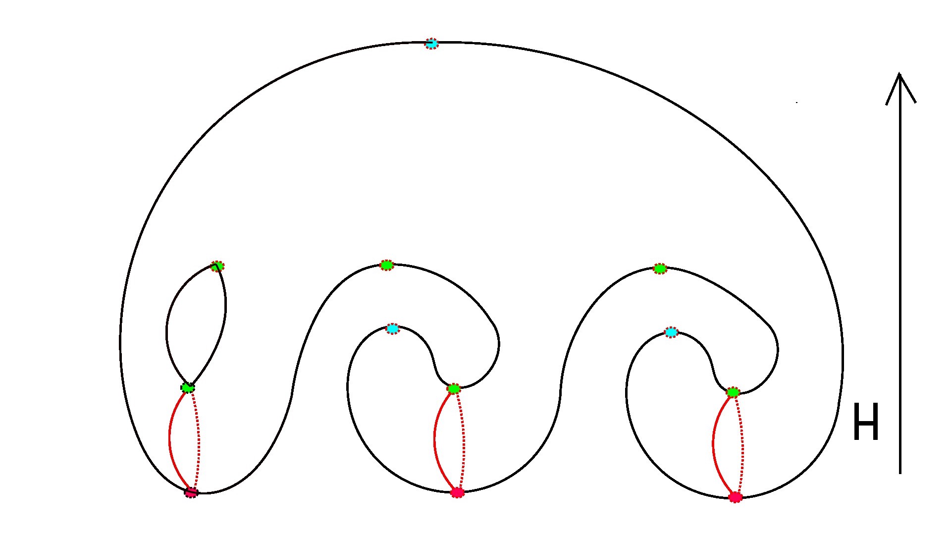
Figure 1: The red circles are the admissible link.

Note that if $\underline{L}$ is admissible, so is $\varphi(\underline{L})$, where $\varphi$ is any Hamiltonian symplecticmorphism. We assume that the link is $\eta$-admissible throughout.

Remark 1.1.

To define $HF(\Sigma,\varphi_{H}(\underline{L}),\underline{L})$, we need stronger assumptions on $\underline{L}$ than [7] for technical reasons.

In the first part of this note, we study the properties of the spectral invariants $c_{\underline{L},\eta}$. The results are summarized in the following theorem. These properties are parallel to the one in [7, 31].

Theorem 1.

The spectral invariant $c_{\underline{L},\eta}:C^{\infty}([0,1]\times\Sigma)\times HF(\Sigma,\underline{L})\to\{-\infty\}\cup\mathbb{R}$ satisfies the following properties:

1. (Spectrality) For any $H$ and $a\neq 0\in HF(\Sigma,\underline{L})$, we have $c_{\underline{L},\eta}(H,a)\in Spec(H:\underline{L})$.

2. (Hofer-Lipschitz) For $a\neq 0\in HF(\Sigma,\underline{L})$, we have

   $$d\int_{0}^{1}\min_{\Sigma}(H_{t}-K_{t})dt\leq c_{\underline{L},\eta}(H,a)-c_{\underline{L},\eta}(K,a)\leq d\int_{0}^{1}\max_{\Sigma}(H_{t}-K_{t})dt.$$

3. (Shift) Fix $a\neq 0\in HF(\Sigma,\underline{L})$. Let $c:[0,1]_{t}\to\mathbb{R}$ be a function only dependent on $t$. Then

   $$c_{\underline{L},\eta}(H+c,a)=c_{\underline{L},\eta}(H,a)+d\int_{0}^{1}c(t)dt.$$

4. (Homotopy invariance) Let $H,K$ are two mean-normalized Hamiltonian functions. Suppose that they are homotopic in the sense of Definition 4.1. Then

   $$c_{\underline{L},\eta}(H,a)=c_{\underline{L},\eta}(K,a).$$

5. (Lagrangian control) If $H_{t}|_{L_{i}}=c_{i}(t)$ for $i=1,..,d$, then

   $$c_{\underline{L},\eta}(H,a)=c_{\underline{L},\eta}(0,a)+\sum_{i=1}^{d}\int_{0}^{1}c_{i}(t)dt.$$

   Moreover, for any Hamiltonian function $H$, we have

   $$\sum_{i=1}^{d}\int_{0}^{1}\min_{L_{i}}H_{t}dt+c_{\underline{L},\eta}(0,a)\leq c_{\underline{L},\eta}(H,a)\leq c_{\underline{L},\eta}(0,a)+\sum_{i=1}^{d}\int_{0}^{1}\max_{L_{i}}H_{t}dt.$$

6. (Triangle inequality) For any Hamiltonian functions $H,K$ and $a,b\in HF(\Sigma,\underline{L})$, we have

   $$c_{\underline{L},\eta}(H\#K,\mu_{2}(a\otimes b))\leq c_{\underline{L},\eta}(H,a)+c_{\underline{L},\eta}(K,b),$$

   where $\mu_{2}$ is the quantum product defined in Section 3.

7. (Normalization) For the unit $e$, we have $c_{\underline{L},\eta}(0,e)=0.$

8. (Calabi property) Let $\{\underline{L}_{m}\}_{m=1}^{\infty}$ be a sequence of $\eta$-admissible links. Suppose that $\{\underline{L}_{m}\}_{m=1}^{\infty}$ is equidistributed in the sense of [7]. Let $d_{m}$ denote the number of components of $\underline{L}_{m}$. Then for $a\neq 0\in HF(\Sigma,\underline{L})$, we have

   $$\lim_{m\to\infty}\frac{1}{d_{m}}\left(c_{\underline{L}_{m},\eta}(H,a)-c_{\underline{L}_{m},\eta}(0,a)\right)=\int_{0}^{1}\int_{\Sigma}H_{t}dt\wedge\omega.$$

Remark 1.2.

At this moment, we haven’t confirmed whether the isomorphism (1.1) is canonical, but we believe that it is true from the view point of tautological correspondence. Also, we don’t know whether the product $\mu_{2}$ agrees with the usual quantum product in monotone Lagrangian Floer homology. So we cannot deduce Theorem 1 from (1.1) and the results in [7, 31] directly. But the methods in the proof of Theorem 1 basically the same as [7, 31].

In [13], we define the closed-open morphisms (1.2). We use the same techniques to construct a “reverse” of the closed-open morphisms, called open-closed morphisms.

Theorem 2.

Let $\underline{L}$ be an admissible link and $\varphi_{H}$ a $d$-nondegenerate Hamiltonian symplecticmorphism. Fix a reference 1–cycle $\gamma_{0}$ with degree $d$ and a base point $\mathbf{x}\in\underline{L}$. Let $\mathcal{Z}_{ref}\in H_{2}(W,{\mathbf{x}}_{H},\gamma_{0})$ be a reference relative homology class. Let $(W,\Omega_{H},\mathcal{L}_{H})$ be the open-closed symplectic cobordism defined in Section 5. Then for a generic admissible almost complex structure $J\in\mathcal{J}(W,\Omega_{H})$, the triple $(W,\Omega_{H},\mathcal{L}_{H})$ induces a homomorphism

$$(\mathcal{OC}_{\mathcal{Z}_{ref}}(W,\Omega_{H},\mathcal{L}_{H})_{J})_{*}:HF(\Sigma,\varphi_{H}(\underline{L}),\underline{L},\mathbf{x})_{J}\to\widetilde{PFH}(\Sigma,\varphi_{H},\gamma_{0})_{J}$$

satisfying the following properties:

• (Partial invariance) Suppose that $\varphi_{H},\varphi_{G}$ satisfy the following conditions: (see Definition 2.1)

  1. Each periodic orbit of $\varphi_{H}$ with degree less than or equal $d$ is either $d$–negative elliptic or hyperbolic.

  2. Each periodic orbit of $\varphi_{G}$ with degree less than or equal $d$ is either $d$–positive elliptic or hyperbolic.

  Fix reference relative homology classes $Z_{ref}\in H_{2}(X,\gamma_{1},\gamma_{0})$, $\mathcal{Z}_{0}\in H_{2}(W,\mathbf{x}_{G},\gamma_{0})$ and $\mathcal{Z}_{1}\in H_{2}(W,\mathbf{x}_{H},\gamma_{1})$ satisfying $A_{ref}\#\mathcal{Z}_{0}=Z_{ref}\#\mathcal{Z}_{1}$, where $A_{ref}$ is the class defining the continuous morphism $\mathcal{I}^{H,G}_{0,0}$. Then for any generic admissible almost complex structures $J_{H}\in\mathcal{J}(W,\Omega_{H})$ and $J_{G}\in\mathcal{J}(W,\Omega_{G})$, we have the following commutative diagram:

  $$\begin{CD}HF_{*}(\Sigma,\varphi_{H}(\underline{L}),\underline{L},\mathbf{x})_{J_{H}}@>{(\mathcal{OC}_{\mathcal{Z}_{1}}(W,\Omega_{H},\mathcal{L}_{H})_{J_{H}})_{*}}>{}>\widetilde{PFH}_{*}(\Sigma,\varphi_{H},\gamma_{1})_{J_{H}}\\ @V{}V{\mathcal{I}^{H,G}_{0,0}}V@V{}V{PFH_{Z_{ref}}^{sw}(X,\Omega_{X})}V\\ HF_{*}(\Sigma,\varphi_{G}(\underline{L}),\underline{L},\mathbf{x})_{J_{G}}@>{(\mathcal{OC}_{\mathcal{Z}_{0}}(W,\Omega_{G},\mathcal{L}_{G})_{J_{G}})_{*}}>{}>\widetilde{PFH}_{*}(\Sigma,\varphi_{G},\gamma_{0})_{J_{G}}\end{CD}$$

  Here $PFH_{Z_{ref}}^{sw}(X,\Omega_{X})$ is the PFH cobordism map induced by symplectic cobordism (2.9) and $\mathcal{I}^{H,G}_{0,0}$ is the continuous morphism on QHF defined in Section 3.

• (Non–vanishing) There are nonzero classes $e_{\diamondsuit}\in HF(\Sigma,\underline{L})$ and $\sigma^{\mathbf{x}}_{\diamondsuit H}\in\widetilde{PFH}(\Sigma,\varphi_{H},\gamma_{H}^{\mathbf{x}})$ such that if $\varphi_{H}$ satisfies the condition ($\spadesuit$.2), then we have

  $$\mathcal{OC}_{\mathcal{Z}_{ref}}(W,\varphi_{H},\mathcal{L}_{H})_{*}((j^{\mathbf{x}}_{H})^{-1}(e_{\diamondsuit}))=\sigma^{\mathbf{x}}_{\diamondsuit H},$$

  where $j_{H}^{\mathbf{x}}$ is the canonical isomorphism (2.14). In particular, the open-closed morphism is non–vanishing.

There is a special class $e\in HF(\Sigma,\underline{L})$ called the unit (see Definition 3.7). Suppose that the link $\underline{L}$ is $0$-admissible. Define spectral invariants

$$\begin{split}&c_{\underline{L}}^{-}(H):=c_{\underline{L},\eta=0}(H,e_{\diamondsuit})\mbox{ \ and \ }c_{\underline{L}}^{+}(H):=c_{\underline{L},\eta=0}(H,e).\end{split}$$

Corollary 1.2.

Suppose that the link $\underline{L}$ is $0$-admissible. For any Hamiltonian function $H$, let $\sigma^{\mathbf{x}}_{\heartsuit H}\in\widetilde{PFH}(\Sigma,\varphi_{H},\gamma_{H}^{\mathbf{x}})$ be the class defined in Section 7 of [13]. We have

$$c^{pfh}_{d}(H,\sigma^{\mathbf{x}}_{\diamondsuit H},\gamma^{\mathbf{x}}_{H})+\int_{0}^{1}H_{t}(\mathbf{x})dt\leq c_{\underline{L}}^{-}(H)\leq c_{\underline{L}}^{+}(H)\leq c^{pfh}_{d}(H,\sigma^{\mathbf{x}}_{\heartsuit H},\gamma^{\mathbf{x}}_{H})+\int_{0}^{1}H_{t}(\mathbf{x})dt,$$

where $\int_{0}^{1}H_{t}(\mathbf{x})dt$ is short for $\sum_{i=1}^{d}\int_{0}^{1}H_{t}(x_{i})dt.$

Corollary 1.3.

Suppose that $\underline{L}$ is $0$-admissible and $\Sigma=\mathbb{S}^{2}$. Then for any Hamiltonian function $H$, we have

$$c^{pfh}_{d}(H,\sigma^{\mathbf{x}}_{\heartsuit H},\gamma_{H}^{\mathbf{x}})+\int_{0}^{1}H_{t}(\mathbf{x})dt-1\leq c_{\underline{L}}^{-}(H)\leq c_{\underline{L}}^{+}(H)\leq c^{pfh}_{d}(H,\sigma^{\mathbf{x}}_{\heartsuit H},\gamma_{H}^{\mathbf{x}})+\int_{0}^{1}H_{t}(\mathbf{x})dt.$$

Moreover, for any $\varphi\in Ham(\mathbb{S}^{2},\omega)$, we have

$$\mu_{\underline{L},\eta=0}(\varphi,e)=\mu_{\underline{L},\eta=0}(\varphi,e_{\diamondsuit})=\mu_{d}^{pfh}(\varphi),$$ (1.3)

where $\mu_{\underline{L},\eta=0},\mu_{d}^{pfh}$ are the homogenized spectral invariants (see Section 6 for details). In particular, for any two $0$-admissible links $\underline{L},\underline{L}^{\prime}$ with same number of components, then we have $\mu_{\underline{L},\eta=0}(\varphi,e)=\mu_{\underline{L}^{\prime},\eta=0}(\varphi,e)=\mu_{\underline{L},\eta=0}(\varphi,e_{\diamondsuit})=\mu_{\underline{L}^{\prime},\eta=0}(\varphi,e_{\diamondsuit})$.

The terms $c^{pfh}_{d}(H,\sigma^{\mathbf{x}}_{\heartsuit H},\gamma_{H}^{\mathbf{x}})+\int_{0}^{1}H_{t}(\textbf{x})dt$, $c^{pfh}_{d}(H,\sigma^{\mathbf{x}}_{\diamondsuit H},\gamma_{H}^{\mathbf{x}})+\int_{0}^{1}H_{t}(\textbf{x})dt$ and $c_{\underline{L},\eta}(H,a)$ are independent of the choice of the base point. See discussion in Section 7 of [13].

Remark 1.3.

For technical reasons, the cobordism maps on PFH are defined by using the Seiberg-Witten theory [28] and the isomorphism “PFH=SWF” [30]. Nevertheless, the proof of the Theorem 2 needs a holomorphic curves definition. The assumptions $\spadesuit$.1, $\spadesuit$.2 are used to guarantee that the PFH cobordism maps can be defined by counting holomorphic curves. According to the results in [11], the Seiberg-Witten definition agrees with the holomorphic curves definition in these special cases. We believe that the assumptions $\spadesuit$.1, $\spadesuit$.2 can be removed if one could define the PFH cobordism maps by pure holomorphic curve methods.

By Proposition 3.7 of [11], the conditions $\spadesuit$.1, $\spadesuit$.2 can be achieved by a $C^{1}$-perturbation of the Hamiltonian functions. More precisely, fix a metric $g_{Y}$ on $S^{1}\times\Sigma$. For any $\delta>0$ and Hamiltonian function $H$, there is a Hamiltonian function $H^{\prime}$ such that

• $\varphi_{H^{\prime}}$ satisfies $\spadesuit$.1 ($\spadesuit$.2).

• $|H^{\prime}-H|+|dH-dH^{\prime}|_{g_{Y}}\leq\delta$.

Even Theorem 2 relies on the conditions $\spadesuit$.1, $\spadesuit$.2 , the above estimates and the Hofer-Lipschitz property imply that Corollaries 1.2, 1.3 work for a general Hamiltonian function.

From [7], we know that the homogenized link spectral invariants are homogeneous quasimorphisms. We show that this is also true for $\mu_{d}^{pfh}(\varphi).$ Recall that a homogeneous quasimorphism on a group $G$ is a map $\mu:G\to\mathbb{R}$ such that

1. $\mu(g^{n})=n\mu(g)$;

2. there exists a constant $D=D(\mu)\geq 0$, called the defect of $\mu$, satisfying

   $$|\mu(gh)-\mu(g)-\mu(h)|\leq D.$$

Theorem 3.

The homogenized spectral invariants $\mu_{d}^{pfh}:Ham(\mathbb{S}^{2},\omega)\to\mathbb{R}$ are homogeneous quasimorphisms with defect $1$.

Relavant results

The Calabi property in Theorem 1 in fact is an analogy of the “ECH volume property” for embedded contact homology, it was first discovered by D. Cristofaro-Gardiner, M. Hutchings, and V. Ramos [3]. Embedded contact homology (short for “ECH”) is a sister version of the periodic Floer homology. The construction of ECH and PFH are the same. The only difference is that they are defined for different geometric structures. If a result holds for one of them, then one could expect that there should be a parallel result for another one. The Calabi property also holds for PFH. This is proved by O. Edtmair and Hutchings [16], also by D. Cristofaro-Gardiner, R. Prasad and B. Zhang [6] independently. The Calabi property for QHF is discovered in [7].

Recently, D. Cristofaro-Gardiner, V. Humili$\grave{e}$re, C. Mak, S. Seyfaddini and I. Smith show that the homogenized link spectral invariants satisfy the “two-terms Weyl law” for a class of automatous Hamiltonian functions [8] on the sphere. We believe that the HF spectral invariants agree with the link spectral invariants. If one could show that this is true, Corollary 1.3 implies that homogenized PFH spectral invariants agree with the homogenized link spectral invariants. This suggests that homogenized PFH spectral invariants should also satisfy the “two-terms Weyl law”.

2 Preliminaries

2.1 Periodic Floer homology

In this section, we review the definition of twisted periodic Floer homology and PFH spectral invariants. For more details, please refer to [20, 21, 4, 16].

Suppose that $\Sigma$ is a closed surface and $\omega$ is a volume form of volume 1. Given a Hamiltonian function $H:S^{1}_{t}\times\Sigma\to\mathbb{R}$, then we have a unique vector field $X_{H_{t}}$, called the Hamiltonian vector field, satisfying the relation $\omega(X_{H_{t}},\cdot)=d_{\Sigma}H_{t}$. Let $\varphi_{H}^{t}$ be the flow generated by $X_{H_{t}}$, i.e., $\partial_{t}\varphi_{H}^{t}=X_{H_{t}}\circ\varphi_{H}^{t}$ and $\varphi_{H}^{0}=id$. For each $t$, $\varphi_{H}^{t}$ is a symplecticmorphism. The time-1 flow is denoted by $\varphi_{H}:=\varphi_{H}^{1}$. A Hamiltonian function is called automatous if it is $t$-independent.

Fix a symplecticmorphism $\varphi$. Define the mapping torus by

$$Y_{\varphi}:=[0,1]_{t}\times\Sigma/(0,\varphi(x))\sim(1,x).$$

There is a natural vector field $R:=\partial_{t}$ and a closed 2-form $\omega_{\varphi}$ on $Y_{\varphi}$ induced from the above quotient. The pair $(dt,\omega_{\varphi})$ forms a stable Hamiltonian structure and $R$ is the Reeb vector field. Let $\xi:=\ker\pi_{*}$ denote the vertical bundle of $\pi:Y_{\varphi}\to S^{1}.$

A periodic orbit is a map $\gamma:\mathbb{R}/q\mathbb{Z}\to Y_{\varphi}$ satisfying the ODE $\partial_{t}\gamma(t)=R\circ\gamma(t)$. The number $q\geq 0$ is called the period or degree of $\gamma$. Note that $q$ is equal to the intersection number $[\gamma]\cdot[\Sigma]$.

A periodic orbit is called nondegenerate if the linearized return map does not have 1 as an eigenvalue. The nondegenerate periodic orbits are classified as either elliptic or hyperbolic according to the eigenvalues of linearized return maps. The symplecticmorphism $\varphi$ is called $d$-nondegenerate if every closed orbit with degree at most $d$ is nondegenerate.

Let $\gamma$ be an elliptic periodic orbit with period $q$. We can find a trivialization of $\xi$ such that the linearized return map is a rotation $e^{i2\pi\theta_{t}}$, where $\{\theta_{t}\}_{t\in[0,q]}$ is a continuous function with $\theta_{0}=0$. The number $\theta=\theta_{t}|_{t=q}\in\mathbb{R}/\mathbb{Z}$ is called the rotation number of $\gamma$ (see [21] for details). The following definition explains the terminologies in the assumptions $\spadesuit$.1, $\spadesuit$.2.

Definition 2.1.

(see [22] Definition 4.1) Fix $d>0$. Let $\gamma$ be an embedded elliptic orbit with degree $q\leq d$.

• $\gamma$ is called $d$-positive elliptic if the rotation number $\theta$ is in $(0,\frac{q}{d})\mod 1$.

• $\gamma$ is called $d$-negative elliptic if the rotation number $\theta$ is in $(-\frac{q}{d},0)\mod 1$.

For our purpose, we assume that $\varphi$ is Hamiltonian throughout (but the construction of PFH works for a general symplecticmorphism). Under the Hamiltonian assumption, we have the following diffeomorphism

$$\begin{split}\Psi_{H}:&S^{1}_{t}\times\Sigma\to Y_{\varphi_{H}}\\ &(s,t,x)\to(s,t,(\varphi_{H}^{t})^{-1}(x)).\end{split}$$ (2.4)

It is easy to check that $\Psi_{H}^{*}(\omega_{\varphi_{H}})=\omega+d(H_{t}dt)$ and $(\Psi_{H})_{*}(\partial_{t}+X_{H})=R$.

PFH complex

An orbit set is a finite set of pairs $\gamma=\{(\gamma_{i},m_{i})\}$, where $\{\gamma_{i}\}$ are distinct embedded periodic orbits and $\{m_{i}\}$ are positive integers. An orbit set is called a PFH generator if it satisfies a further condition: If $\gamma_{i}$ is hyperbolic, then $m_{i}=1$.

Let $H_{2}(Y_{\varphi},\gamma_{+},\gamma_{-})$ denote the set of 2-chains $Z$ in $Y_{\varphi}$ with $\partial Z=\gamma_{+}-\gamma_{-}$, modulo the boundary of 3-chains. We call the element $Z\in H_{2}(Y_{\varphi},\gamma_{+},\gamma_{-})$ a relative homology classes. This an affine space of $H_{2}(Y_{\varphi},\mathbb{Z})\cong\mathbb{Z}[\Sigma]\oplus(H_{1}(S^{1})\otimes H_{1}(\Sigma))$.

For a relative homology class $Z\in H_{2}(Y_{\varphi},\gamma_{+},\gamma_{-})$, Hutchings defines a topology index called $J_{0}$ index [19] that measure the topology complexity of the curves. Fix a trivialization $\tau$ of $\xi$. The $J_{0}$ index is given by the following formula:

$$J_{0}(Z):=-c_{\tau}(\xi|_{Z})+Q_{\tau}(Z)+\sum_{i}\sum_{p=1}^{m_{i}-1}CZ_{\tau}(\gamma_{+,i}^{p})-\sum_{j}\sum_{q=1}^{n_{j}-1}CZ_{\tau}(\gamma_{-,j}^{q}),$$

where $c_{\tau}(\xi|_{Z})$ is the relative Chern number, $Q_{\tau}(Z)$ is the relative self-intersection number and $CZ_{\tau}$ is the Conley-Zehnder index.

There is another topological index called ECH index. It is defined by

$$I(Z):=c_{\tau}(\xi|_{Z})+Q_{\tau}(Z)+\sum_{i}\sum_{p=1}^{m_{i}}CZ_{\tau}(\gamma_{+,i}^{p})-\sum_{j}\sum_{q=1}^{n_{j}}CZ_{\tau}(\gamma_{-,j}^{q}).$$

We refer readers to [18, 19] for more details on $I$ and $J_{0}$.

Fix a reference 1-cycle $\gamma_{0}$ transversed to $\xi$ positively. Assume that $[\gamma_{0}]\cdot[\Sigma]>g(\Sigma)$ throughout. An anchored orbit set is a pair $(\gamma,[Z])$, where $\gamma$ is an orbit set and $[Z]\in H_{2}(Y_{\varphi},\gamma_{+},\gamma_{-})/\ker(\omega_{\varphi}+\eta J_{0})$. We call it an anchored PFH generator if $\gamma$ is a PFH generator. Note that $H_{2}(Y_{\varphi},\gamma_{+},\gamma_{-})/\ker(\omega_{\varphi}+\eta J_{0})$ is an affine space of $\mathbb{Z}[\Sigma]$.

The chain complex $\widetilde{PFC}(\Sigma,\varphi,\gamma_{0})$ is the set of the formal sums (possibly infinity)

$$\sum a_{(\gamma,[Z])}(\gamma,[Z]),$$ (2.5)

where $a_{(\gamma,[Z])}\in\mathbb{Z}/2\mathbb{Z}$ and each $(\gamma,[Z])$ is an anchored PFH generator. Also, for any $C\in\mathbb{R}$, we require that there is only finitely many $(\gamma,[Z])$ such that $\int_{Z}\omega_{\varphi_{H}}>C$ and $a_{(\gamma,[Z])}\neq 0$.

Let $\Lambda=\{\sum_{i}a_{i}q^{b_{i}}|a_{i}\in\mathbb{Z}/2\mathbb{Z},b_{0}<b_{1}...\}$ be the Novikov ring. Then the $\widetilde{PFC}(\Sigma,\varphi,\gamma_{0})$ is $\Lambda$-module because we define an action

$$\left(\sum_{i}a_{i}q^{b_{i}}\right)\cdot(\gamma,[Z]):=\sum_{i}a_{i}(\gamma,[Z-b_{i}\Sigma]).$$ (2.6)

In most of the time, it is convenient to take

$$\gamma_{0}=\Psi_{H}(S^{1}\times\textbf{x}),$$ (2.7)

denoted by $\gamma_{H}^{\textbf{x}}$, where $\textbf{x}=(x_{1},...x_{d})$ is $d$-points on $\Sigma$ (not necessarily to be distinct).

Differential on PFH

To define the differential, consider the symplectization

$$X:=\mathbb{R}_{s}\times Y_{\varphi},\ \ \Omega:=\omega_{\varphi}+ds\wedge dt.$$

An almost complex structure on $X$ is called admissible if it preserves $\xi$, is $\mathbb{R}$-invariant, sends $\partial_{s}$ to $R$, and its restriction to $\xi$ is compatible with $\omega_{\varphi}$. The set of admissible almost complex structures is denoted by $\mathcal{J}(Y_{\varphi},\omega_{\varphi})$.

Given $J\in\mathcal{J}(Y_{\varphi},\omega_{\varphi})$ and orbit sets $\gamma_{+}=\{(\gamma_{+,i},m_{i})\}$, $\gamma_{-}=\{(\gamma_{-,j},n_{j})\}$, let $\mathcal{M}^{J}(\gamma_{+},\gamma_{-},Z)$ be the moduli space of punctured holomorphic curves $u:\dot{F}\to X$ with the following properties: $u$ has positive ends at covers of $\gamma_{+,i}$ with total multiplicity $m_{i}$, negative ends at covers of $\gamma_{-,j}$ with total multiplicity $n_{j}$, and no other ends. Also, the relative homology class of $u$ is $Z$. Note that $\mathcal{M}^{J}(\gamma_{+},\gamma_{-},Z)$ admits a natural $\mathbb{R}$-action.

The differential $\partial_{J}$ on $\widetilde{PFC}(\Sigma,\varphi,\gamma_{0})$ is defined by

$$\partial_{J}(\gamma_{+},[Z_{+}]):=\sum_{\gamma_{-}}\sum_{Z,I(Z)=1}\#\left(\mathcal{M}^{J}(\gamma_{+},\gamma_{-},Z)/\mathbb{R}\right)(\gamma_{-},[Z_{+}-Z]).$$

The homology of $(\widetilde{PFC}(\Sigma,\varphi,\gamma_{0}),\partial_{J})$ is called the twisted periodic Floer homology, denoted by $\widetilde{PFH}(\Sigma,\varphi,\gamma_{0})_{J}$. By Corollary 1.1 of [30], PFH is independent of the choice of almost complex structures and Hamiltonian isotopic of $\varphi$. Note that $\widetilde{PFH}(\Sigma,\varphi,\gamma_{0})$ is a $\Lambda$-module because the action (2.6) descends to the homology.

The U-map

There is a well-defined map

$$U:\widetilde{PFH}(\Sigma,\varphi_{H},\gamma_{0})\to\widetilde{PFH}(\Sigma,\varphi_{H},\gamma_{0}).$$

Fix $z\in\mathbb{R}\times Y_{\varphi_{H}}$. The definition of the U-map is similar to the differential. Instead of counting $I=1$ holomorphic curves modulo $\mathbb{R}$ translation, the U-map is defined by counting $I=2$ holomorphic curves that pass through the fixed point $z$ and modulo $\mathbb{R}$ translation. The homotopy argument can show that the U-map is independent of the choice of $z$. For more details, please see Section 2.5 of [26].

Cobordism maps on PFH

Let $(X,\Omega_{X})$ be a symplectic 4-manifold. Suppose that there exists a compact subset $K$ such that

$$(X-K,\Omega_{X})\cong\left([0,\infty)\times Y_{\varphi_{+}},\omega_{\varphi_{+}}+ds\wedge dt\right)\cup\left((-\infty,0]\times Y_{\varphi_{-}},\omega_{\varphi_{-}}+ds\wedge dt\right)$$ (2.8)

We allow $Y_{\varphi_{+}}=\emptyset$ or $Y_{\varphi_{-}}=\emptyset$. We call $(X,\Omega_{X})$ a symplectic cobordism from $(Y_{\varphi_{+}},\omega_{\varphi_{+}})$ to $(Y_{\varphi_{-}},\omega_{\varphi_{-}})$. Fix a reference homology class $Z_{ref}\in H_{2}(X,\gamma_{0},\gamma_{1})$. The symplectic manifold $(X,\Omega_{X})$ induces a homomorphism

$$PFH_{Z_{ref}}^{sw}(X,\Omega_{X}):\widetilde{PFH}(\Sigma,\varphi_{+},\gamma_{0})\to\widetilde{PFH}(\Sigma,\varphi_{-},\gamma_{1}).$$

This homomorphism is called a PFH cobordism map.

Following Hutchings-Taubes’s idea [23], the cobordism map $PFH_{Z_{ref}}^{sw}(X,\Omega_{X})$ is defined by using the Seiberg-Witten theory [28] and Lee-Taubes’s isomorphism [30]. Even the cobordism maps are defined by Seiberg-Witten theory, they satisfy some nice properties called holomorphic curves axioms. It means that the PFH cobordism maps count holomorphic curves in certain sense. For the precise statement, we refer readers to [11] and Appendix of [13].

In this paper, we will focus on the following special cases of $(X,\Omega_{X})$.

1. Given two Hamiltonian functions $H_{+},H_{-}$, define a homotopy $H_{s}:=\chi(s)H_{+}+(1-\chi(s))H_{-}$, where $\chi$ is a cut off function such that $\chi=1$ for $s\geq R_{0}>0$ and and $\chi=0$ for $\chi\leq 0$. Define

   $$\begin{split}&X:=\mathbb{R}_{s}\times S^{1}_{t}\times\Sigma,\\ &\omega_{X}:=\omega+dH_{s}\wedge dt,\ \ \Omega_{X}:=\omega_{X}+ds\wedge dt.\end{split}$$ (2.9)

   This is a symplectic cobordism if $R_{0}$ is sufficiently large. Note that we identify $Y_{\varphi_{H_{\pm}}}$ with $S^{1}\times\Sigma$ implicitly by using (2.4). Fix a reference relative homology class $Z_{ref}\in H_{2}(X,\gamma_{0},\gamma_{1})$. Then we have a cobordism map

   $$PFH_{Z_{ref}}^{sw}(X,\Omega_{X}):\widetilde{PFH}(\Sigma,\varphi_{H_{+}},\gamma_{0})\to\widetilde{PFH}(\Sigma,\varphi_{H_{-}},\gamma_{1}).$$

   This map only depends on $H_{+}$, $H_{-}$ and the relative homology class $Z_{ref}$.

2. Let $(B_{-},\omega_{B_{-}},j_{B_{-}})$ be a sphere with a puncture $p$. Suppose that we have neighbourhood $U$ of $p$ so that we have the following identification

   $$(B_{-},\omega_{B_{-}},j_{B_{-}})|_{U}\cong([0,\infty)_{s}\times S_{t}^{1},ds\wedge dt,j),$$

   where $j$ is a complex structure that maps $\partial_{s}$ to $\partial_{t}$. Let $\chi:\mathbb{R}\to\mathbb{R}$ be cut off function such that $\chi=1$ when $s\geq R_{0}$ and $\chi(s)=0$ when $s\leq R_{0}/10$. Take

   $$\begin{split}&X_{-}=:B_{-}\times\Sigma\\ &\omega_{X_{-}}:=\omega+d(\chi(s)Hdt)\ \ \Omega_{X_{-}}:=\omega_{X_{-}}+\omega_{B_{-}}.\end{split}$$ (2.10)

   For sufficiently large $R_{0}>0$, $(X_{-},\Omega_{X_{-}})$ is a symplectic manifold satisfying (2.8).

In the case (2.9), if $H_{+}$ satisfies $\spadesuit$.1 and $H_{-}$ satisfies $\spadesuit$.2, the author shows that the cobordism map $PFH_{Z_{ref}}^{sw}(X,\Omega_{X})$ can be defined alternatively by using the pure holomorphic curve methods [11]. The holomorphic curves definition will be used to prove Theorem 2. That is why we need the assumptions $\spadesuit$.1, $\spadesuit$.2 in the statement.

Filtered PFH

We define a functional $\mathbb{A}^{\eta}_{H}$ on the anchored orbit sets deformed by the $J_{0}$ index as follows:

$$\mathbb{A}^{\eta}_{H}(\gamma,[Z]):=\int_{Z}\omega_{\varphi}+\eta J_{0}(Z).$$

When $\eta=0$, we write $\mathbb{A}_{H}(\gamma,[Z]):=\mathbb{A}^{\eta=0}_{H}(\gamma,[Z])$ for short. Even through we add an perturbation term to the usual action functional, this still give us a filtration on the PFH complex .

Lemma 2.2 (Lemma 2.4 of [13]).

Let $J\in\mathcal{J}(Y_{\varphi},\omega_{\varphi})$ be an admissible almost complex structure in the symplectization of $\mathbb{R}\times Y_{\varphi}$. Let $\mathcal{C}\in\mathcal{M}^{J}(\alpha_{+},\alpha_{-})$ be a holomorphic current in $\mathbb{R}\times Y_{\varphi}$ without closed component. Then $J_{0}(\mathcal{C})\geq 0$.

Let $\widetilde{PFC}^{L}(\Sigma,\varphi,\gamma_{0})$ be the set of formal sum (2.5) satisfying $\mathbb{A}^{\eta}_{H}(\gamma,[Z])<L$. By Lemma 2.2, this is a subcomplex of $(\widetilde{PFC}(\Sigma,\varphi,\gamma_{0}),\partial_{J})$. The homology is denoted by $\widetilde{PFH}^{L}(\Sigma,\varphi,\gamma_{0})$. Let $\mathfrak{i}_{L}:\widetilde{PFH}^{L}(\Sigma,\varphi,\gamma_{0})\to\widetilde{PFH}(\Sigma,\varphi,\gamma_{0})$ be the map induced by the inclusion.

Take $\eta=0$. Fix $\sigma\in\widetilde{PFH}(\Sigma,\varphi,\gamma_{0})$. The PFH spectral invariant is defined by

$$c_{d}^{pfh}(H,\sigma,\gamma_{0},J):=\inf\{L\in\mathbb{R}|\sigma\mbox{ belongs to the image of }\mathfrak{i}_{L}\}.$$

If $\varphi_{H}$ is degenerate , we define

$$c_{d}^{pfh}(H,\sigma,\gamma_{0})=\lim_{n\to\infty}c_{d}^{pfh}(H_{n},\sigma_{n},\gamma_{0}),$$ (2.11)

where $\varphi_{H_{n}}$ are $d$-nondegenerate, $\{H_{n}\}_{n=1}^{\infty}$ $C^{\infty}$-converges to $H$, and $\sigma_{n}\in\widetilde{PFH}(\Sigma,\varphi_{H_{n}},\gamma_{0})$ is the class corresponding to $\sigma$.

One could define the PFH spectral invariants using $\mathbb{A}^{\eta}_{H}$ for $\eta>0$, however, we cannot prove the Hofer-Lipschitz property by using the methods in [4]. This is because Lemma 2.2 is not true for holomorphic currents in the symplectic cobordisms.

2.2 Quantitative Heegaard Floer homology

In this section, we review the cylindrical formulation of QHF defined in [13].

2.2.1 Cylinderical formulation of QHF

Fix an admissible link $\underline{L}=\cup_{i=1}^{d}L_{i}$ and a Hamiltonian symplecticmorphism $\varphi_{H}$. We always assume that $\varphi_{H}$ is nondegenerate in the sense that $\varphi_{H}(\underline{L})$ intersects $\underline{L}$ transversely.

A Reeb chord of $\varphi_{H}$ is a $d$-union of paths

$$\mathbf{y}=[0,1]\times(y_{1},...y_{d})\subset[0,1]\times\Sigma,$$

where $y_{i}\in L_{i}\cap\varphi_{H}(L_{\sigma(i)})$ and $\sigma:\{1,...,d\}\to\{1,...,d\}$ is a permutation. Obviously, a Reeb chord is determined by $d$-distinct intersection points $(y_{1},...y_{d})$. Thus, we don’t distinguish the Reeb chords and $d$-intersection points.

Fix a base point $\textbf{x}=(x_{1},\cdots x_{d})$, where $x_{i}\in L_{i}$. Define a reference chord

$$\textbf{x}_{H}(t)=\varphi_{H}\circ(\varphi_{H}^{t})^{-1}(\textbf{x})\subset[0,1]_{t}\times\Sigma$$

from $\{0\}\times\varphi_{H}(\underline{L})$ to $\{1\}\times\underline{L}$.

Let $(E:=\mathbb{R}_{s}\times[0,1]_{t}\times\Sigma,\Omega:=\omega+ds\wedge dt)$ be a symplectic manifold. Let $\mathcal{L}=\mathbb{R}\times(\{0\}\times\varphi_{H}(\underline{L})\cup\{1\}\times\underline{L})$ be a union of Lagrangian submanifolds in $(E,\Omega)$. Let $\textbf{y}_{\pm}$ be two Reeb chords. Then we have a concept called $d$-multisection in $E$. Roughly speaking, this is a map $u:\dot{F}\to E$ which is asymptotic to $\textbf{y}_{\pm}$ as $s\to\pm\infty$ and satisfies the Lagrangian boundary conditions, where $\dot{F}$ is a Riemann surface with boundary punctures. If a $d$-multisection is holomorphic, we call it an HF curve. The set of equivalence classes of the $d$-multisections is denoted by $H_{2}(E,\textbf{y}_{+},\textbf{y}_{-})$. An element in $H_{2}(E,\textbf{y}_{+},\textbf{y}_{-})$ is also called a relative homology class. Fix $A\in H_{2}(E,\textbf{y}_{+},\textbf{y}_{-})$. The ECH index and $J_{0}$ index also can be generalized to the current setting, denoted by $I(A)$ and $J_{0}(A)$ respectively. The definition of relative homology class, HF curves and ECH index will be postponed to Section 3. We will define these concepts for a slightly general setting.

Given a Reeb chord y, a capping of y is an equivalence class $[A]$ in $H_{2}(E,\textbf{x}_{H},\textbf{y})/\ker(\omega+\eta J_{0})$. Define the complex ${CF}(\Sigma,\varphi_{H}(\underline{L}),\underline{L},\textbf{x})$ be the set of formal sums of capping

$$\sum_{(y,[A])}a_{(\mathbf{y},[A])}(\mathbf{y},[A])$$ (2.12)

satisfying that $a_{(\mathbf{y},[A])}\in\mathbb{Z}/2\mathbb{Z}$ and for any $C\in\mathbb{R}$, there are only finitely $(\mathbf{y},[A])$ such that $-\int_{A}\omega>C$ and $a_{(\mathbf{y},[A])}\neq 0$.

For $1\leq i\leq k$, let $v_{i}:[0,1]_{s}\times[0,1]_{t}\to\Sigma$ be a map such that $v_{i}(0,t)=v_{i}(1,t)=v_{i}(s,0)=x_{i}$ and $v_{i}(s,1)\in L_{i}$ and represents the class $[B_{i}]\in H_{2}(\Sigma,L_{i},\mathbb{Z})$. Define

$$\begin{split}u_{x_{i}}:&[0,1]_{s}\times[0,1]_{t}\to[0,1]_{s}\times[0,1]_{t}\times\Sigma\\ &(s,t)\to(s,t,\varphi_{H}\circ(\varphi_{H}^{t})^{-1}\circ v_{i}(s,t)).\end{split}$$

Together with the trivial strip at $x_{j}$ $(j\neq i)$, $u_{x_{i}}$ represents a class in $H_{2}(E,\textbf{x}_{H},\textbf{x}_{H})$, still denoted by $[B_{i}]$. We also replace the map $v_{i}$ by $v_{i}^{\prime}$, where $v_{i}^{\prime}$ satisfies $v^{\prime}_{i}(0,t)=v^{\prime}_{i}(1,t)=v^{\prime}_{i}(s,1)=x_{i}$ and $v^{\prime}_{i}(s,0)\in L_{i}$ and represents the class $[B_{i}]\in H_{2}(\Sigma,L_{i})$. Using the same construction, we have another map $u_{x_{i}}^{\prime}$. The slightly different between $u_{x_{i}}$ and $u_{x_{i}}^{\prime}$ is that $u_{x_{i}}|_{t=1}$ wraps $\partial B_{i}$ one time while $u^{\prime}_{x_{i}}|_{t=0}$ wraps $\partial\varphi_{H}(B_{i})$ one time. So we denote the equivalence class of $u_{x_{i}}^{\prime}$ in $H_{2}(E,\textbf{x}_{H},\textbf{x}_{H})$ by $[\varphi_{H}(B_{i})]$. By the monotone assumption (A.4), all the classes $[B_{i}]$ and $[\varphi_{H}(B_{i})]$ are equivalent in $H_{2}(E,\textbf{x}_{H},\textbf{x}_{H})/\ker(\omega+\eta J_{0})$, written as $\mathcal{B}$.

Let $R=\{\sum_{i}a_{i}T^{b_{i}}|a_{i}\in\mathbb{Z}/2\mathbb{Z},b_{0}<b_{1}...\}$ be the Novikov ring. To distinguish the one for PFH, we use different notations to denote the ring and the formal variable. Then $CF(\Sigma,\varphi_{H}(\underline{L}),\underline{L},\textbf{x})$ is a $R$-module because we have the following action

$$\sum_{i}a_{i}T^{b_{i}}\cdot(\textbf{y},[A]):=\sum_{i}a_{i}(\mathbf{y},[A]+b_{i}\mathcal{B}).$$ (2.13)

Let $\mathcal{J}_{E}$ denote the set of $\Omega$-compatible almost complex structures satisfying that $J$ is $\mathbb{R}_{s}$-invariant, $J(\partial_{s})=\partial_{t}$, $J$ sends $T\Sigma$ to itself and $J|_{T\Sigma}$ is $\omega$-compatible. Fix $J\in\mathcal{J}_{E}$. Let $\mathcal{M}^{J}(\textbf{y}_{+},\textbf{y}_{-},A)$ denote the moduli space of HF curves that are asymptotic to $\textbf{y}_{\pm}$ as $s\to\pm\infty$ and have relative homology class $A$. Because $J$ is $\mathbb{R}_{s}$-invariant, this induces a natural $\mathbb{R}$-action on $\mathcal{M}^{J}(\textbf{y}_{+},\textbf{y}_{-},A)$.

Fix a generic $J\in\mathcal{J}_{E}$. The differential is defined by

$$d_{J}(\textbf{y}_{+},[A_{+}])=\sum_{A\in H_{2}(E,\textbf{y}_{+},\textbf{y}_{-}),I(A)=1}\#\left(\mathcal{M}^{J}(\textbf{y}_{+},\textbf{y}_{-},A)/\mathbb{R}\right)(\textbf{y}_{-},[A_{+}\#A]).$$

The homology of $(CF_{*}(\Sigma,\varphi_{H}(\underline{L}),\underline{L},\textbf{x}),d_{J})$ is well defined [13], denoted by $HF_{*}(\Sigma,\varphi_{H}(\underline{L}),\underline{L},\textbf{x})_{J}$. Again, the Floer homology is a $R$-module.

By Proposition 3.9 of [13], the homology is independent of the choices of $J$ and $H$. For different choices of $(J,H)$, there is an isomorphism between the corresponding QHF called a continuous morphism. More details about this point are given in Section 3 later. For two different choices of base points, the corresponding homologies are also isomorphic. Let $HF(\Sigma,\underline{L})$ be the direct limit of the continuous morphisms. For any $H$, we have an isomorphism

$$j_{H}^{\mathbf{x}}:HF(\Sigma,\varphi_{H}(\underline{L}),\underline{L},\mathbf{x})\to HF(\Sigma,\underline{L}).$$ (2.14)

Combining the isomorphism (1.1) with Lemma 6.10 of [7], we know that $HF_{*}(\Sigma,\underline{L})$ is isomorphic to $H^{*}(\mathbb{T}^{d},R)$ as an $R$-vector space, where $\mathbb{T}^{d}$ is the $d$-torus.

Remark 2.1.

Even though we only define the QHF for a Hamiltonian symplecticmorphism $\varphi_{H}$, the above construction also works for a pair of Hamiltonian symplecticmorphisms $(\varphi_{H},\varphi_{K})$. Because $\varphi_{K}(\underline{L})$ is also an admissible link, we just need to replace $\underline{L}$ by $\varphi_{K}(\underline{L})$. The result is denoted by $HF(\Sigma,\varphi_{H}(\underline{L}),\varphi_{K}(\underline{L}),\mathbf{x})$.

2.2.2 Filtered QFH and spectral invariants

Similar as [31, 7], we define an action functional on the generators by

$$\mathcal{A}^{\eta}_{H}(\textbf{y},[A]):=-\int_{A}\omega+\int_{0}^{1}H_{t}(\textbf{x})dt-\eta J_{0}(A).$$

We remark that the term $J_{0}(A)$ is corresponding to the $\Delta\cdot[\hat{\mathbf{y}}]$ in [7],where $\Delta$ is the diagonal of $Sym^{d}\Sigma$ and $\hat{\mathbf{y}}$ is a capping of a Reeb chord $\mathbf{y}$. This view point is proved in Proposition 4.2 in [13].

Let $CF^{L}(\Sigma,\varphi_{H}(\underline{L}),\underline{L},\mathbf{x})$ be the set of formal sums (2.13) satisfying $\mathcal{A}^{\eta}_{H}(\textbf{y},[A])<L$. It is easy to check that it is a subcomplex. The filtered QHF, denoted by $HF^{L}(\Sigma,\varphi_{H}(\underline{L}),\underline{L})$, is the homology $(CF^{L}(\Sigma,\varphi_{H}(\underline{L}),\underline{L}),d_{J})$. Let

$$i_{L}:HF^{L}(\Sigma,\varphi_{H}(\underline{L}),\underline{L},\mathbf{x})\to HF(\Sigma,\varphi_{H}(\underline{L}),\underline{L},\mathbf{x})$$

be the homomorphism induced by the inclusion.

Definition 2.3.

Fix $a\in HF(\Sigma,\underline{L})$. The HF spectral invariant is

$$c_{\underline{L},\eta}(H,a):=\inf\{L\in\mathbb{R}|(j_{H}^{\mathbf{x}})^{-1}(a)\mbox{ belongs to the image of }i_{L}\}.$$

Let $\textbf{c}=\sum a_{(\textbf{y},[A])}(\textbf{y},[A])$ be a cycle in $CF(\Sigma,\varphi_{H}(\underline{L}),\underline{L},\mathbf{x}).$ The action of this cycle is defined by

$$\mathcal{A}^{\eta}_{H}(\textbf{c})=\max\{\mathcal{A}^{\eta}_{H}(\textbf{y},[A])|a_{(\textbf{y},[A])}\neq 0\}.$$

Then the spectral invariant can be expressed alternatively as

$$c_{\underline{L},\eta}(H,a)=\inf\{\mathcal{A}^{\eta}_{H}(\textbf{c})|[\textbf{c}]=(j_{H}^{\mathbf{x}})^{-1}(a)\}.$$ (2.15)

Let $HF(Sym^{d}\Sigma,Sym^{d}\underline{L},Sym^{d}\varphi_{H})$ denote the QHF defined in [7]. Because QHF is independent of the choices of $\varphi_{H}$ and $\mathbf{x}$, we have an abstract group $HF(Sym^{d}\underline{L})$ and a canonical isomorphism

$$\mathbf{j}_{H}^{\mathbf{x}}:HF(Sym^{d}\Sigma,Sym^{d}\underline{L},Sym^{d}\varphi_{H})\to HF(Sym^{d}\underline{L}).$$

Since the isomorphism (1.1) also preserves the action filtrations, we have

$$\frac{1}{d}c_{\underline{L},\eta}(H,a)=c^{link}_{\underline{L},\eta}(H,\mathbf{j}^{\textbf{x}}_{H}\circ\Phi_{H}\circ(j_{H}^{\mathbf{x}})^{-1}(a)).$$ (2.16)

We want to emphasize that the isomorphism $\mathbf{j}^{\textbf{x}}_{H}\circ\Phi_{H}\circ(j_{H}^{\mathbf{x}})^{-1}:HF(\Sigma,\underline{L})\to HF(Sym^{d}\underline{L})$ may depend on $H$ and $\mathbf{x}$ a priori. Therefore, the relation (2.16) is not strong enough to transfer all the properties of $c^{link}_{\underline{L}}$ to $c_{\underline{L}}$.

3 Morphisms on HF

In this section, we define the continuous morphisms, quantum product and unit on $HF(\Sigma,\underline{L})$.

3.1 Moduli space of HF curves

In this subsection, we give the definition of HF curves, relative homology class, and the ECH index.

Let $D_{m}$ be a disk with boundary punctures $(p_{0},p_{1},...,p_{m})$, the order of the punctures is counter-clockwise. See Figure 2. Let $\partial_{i}D_{m}$ denote the boundary of $D_{m}$ connecting $p_{i-1}$ and $p_{i}$ for $1\leq i\leq m$. Let $\partial_{m+1}D_{m}$ be the boundary connecting $p_{m}$ and $p_{0}$.

Fix a complex structure $j_{m}$ and a Kähler form $\omega_{D_{m}}$ over $D_{m}$ throughout. We say that $D_{m}$ is a disk with strip-like ends if for each $p_{i}$ we have a neighborhood $U_{i}$ of $p_{i}$ such that

$$(U_{i},\omega_{D_{m}},j_{m})\cong(\mathbb{R}_{\epsilon_{i}}\times[0,1],ds\wedge dt,j),$$ (3.17)

where $j$ is the standard complex structure on $\mathbb{R}\times[0,1]$ that $j(\partial_{s})=\partial_{t}$, where $\epsilon_{i}=+$ for $1\leq i\leq m$ and $\epsilon_{0}=-$. Here $\mathbb{R}_{+}=[0,\infty)$ and $\mathbb{R}_{-}=(-\infty,0]$.

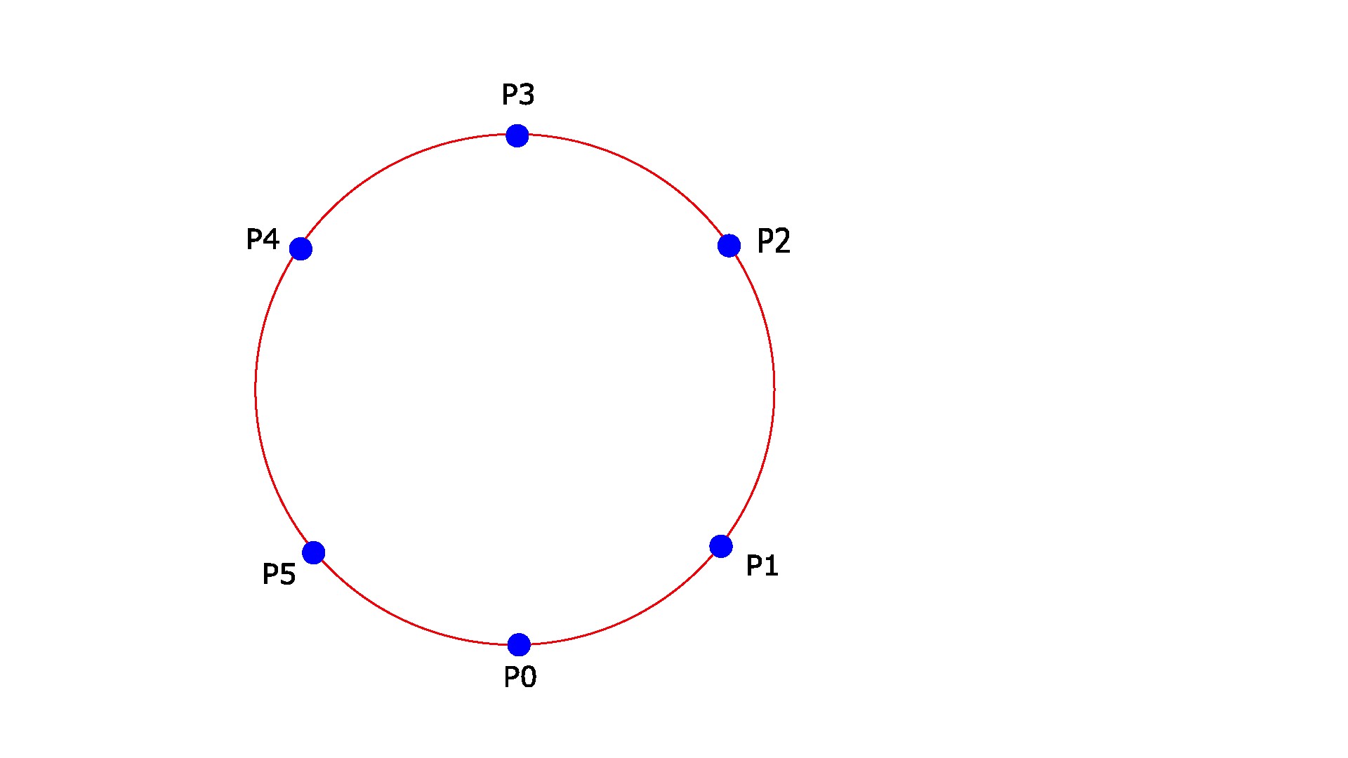
Figure 2: A picture of the case $m=5$.

Let $\pi:E_{m}=D_{m}\times\Sigma\to D_{m}$ be the trivial fibration. A closed 2-form $\omega_{E_{m}}$ is called admissible if $\omega_{E_{m}}|_{\Sigma}=\omega$ and $\omega_{E_{m}}=\omega$ over the strip-like ends. Note that $\Omega_{E_{m}}=\omega_{E_{m}}+\omega_{D_{m}}$ is a symplectic form on $E_{m}$ if $\omega_{D_{m}}$ is large enough. As a result, $(\pi:E_{m}\to D_{m},\Omega_{m})$ over $U_{i}$ can be identified with

$$(\pi:U_{i}\times\Sigma\to U_{i},\Omega_{D_{m}})\cong(\pi_{\mathbb{R}\times[0,1]}:\mathbb{R}_{\epsilon_{i}}\times[0,1]\times\Sigma\to\mathbb{R}_{\epsilon_{i}}\times[0,1],\omega+ds\wedge dt).$$ (3.18)

We call it a (strip-like) end of $(E_{m},\Omega_{E_{m}})$ at $p_{i}$.

Let $\mathcal{L}=(\mathcal{L}_{1},...\mathcal{L}_{m+1})$ be a chain of $d$-disjoint union Lagrangian submanifolds in $\partial E_{m}$ satisfying the following conditions:

1. Let $\mathcal{L}_{i}=\mathcal{L}|_{\partial_{i}D_{m}}\subset\pi^{-1}(\partial_{i}D_{m})$. $\mathcal{L}_{i}$ consists of $d$-disjoint union of Lagrangian submanifolds.

2. For $1\leq i\leq m$, over the end at $p_{i}$ (under the identification 3.18), we have

   $$\mathcal{L}=(\mathbb{R}_{+}\times\{0\}\times\underline{L}_{p_{i-1}})\cup(\mathbb{R}_{+}\times\{1\}\times\underline{L}_{p_{i}}).$$

3. Over the end at $p_{0}$ (under the identification 3.18), we have

   $$\mathcal{L}=(\mathbb{R}_{-}\times\{0\}\times\underline{L}_{p_{0}})\cup(\mathbb{R}_{-}\times\{1\}\times\underline{L}_{p_{m}}).$$

4. The links $\{\underline{L}_{p_{i}}\}_{i=0}^{m}$ are $\eta$-admissible and they are Hamiltonian isotropic to each other.

5. For $z\in\partial D_{m}$, $\mathcal{L}\cap\pi^{-1}(z)$ is an admissible link.

Let $(E_{m},\Omega_{m},\mathcal{L}_{m})$ and $(E_{n},\Omega_{n},\mathcal{L}_{n})$ be two symplectic fibrations. Suppose that the negative end of $(E_{m},\Omega_{m},\mathcal{L}_{m})$ agrees with the $i$-th positive end of $(E_{n},\Omega_{n},\mathcal{L}_{n})$, i.e,

$$\begin{split}&(E_{m},\Omega_{m},\mathcal{L}_{m})|_{U_{0}}\cong(\mathbb{R}_{s_{-}\leq 0}\times[0,1]_{t}\times\Sigma,\omega+ds_{-}\wedge dt,\mathbb{R}_{s_{-}\leq 0}\times(\{0\}\times\underline{L}_{0}\cup\{1\}\times\underline{L}_{1}))\\ &(E_{n},\Omega_{n},\mathcal{L}_{n})|_{U_{i}}\cong(\mathbb{R}_{s_{+}\geq 0}\times[0,1]_{t}\times\Sigma,\omega+ds_{+}\wedge dt,\mathbb{R}_{s_{+}\geq 0}\times(\{0\}\times\underline{L}_{0}\cup\{1\}\times\underline{L}_{1})).\end{split}$$

Fix $R\geq 0$. Define the $R$-stretched composition $(E,\Omega,\mathcal{L}):=(E_{n},\Omega_{n},\mathcal{L}_{n})\circ_{R}(E_{m},\Omega_{m},\mathcal{L}_{m})$ by

$$(E,\Omega,\mathcal{L})=(E_{n},\Omega_{n},\mathcal{L}_{n})|_{s_{+}\leq R}\cup_{s_{+}-R=s_{-}+R}(E_{m},\Omega_{m},\mathcal{L}_{m})|_{s_{-}\geq-R}.$$ (3.19)

In most of the time, the number $R$ is not important, we suppress it from the notation.

Definition 3.1.

Fix Reeb chords $\mathbf{y}_{i}\in\underline{L}_{p_{i-1}}\cap\underline{L}_{p_{i}}$ and $\mathbf{y}_{0}\in\underline{L}_{p_{0}}\cap\underline{L}_{p_{m}}$. Let $(\dot{F},j)$ be a Riemann surface (possibly disconnected) with boundary punctures. A d–multisection is a smooth map $u:(\dot{F},\partial\dot{F})\to E_{m}$ such that

1. $u(\partial{\dot{F}})\subset\mathcal{L}$. Let $\{L_{j}^{i}\}_{i=1}^{d}$ be the connected components of $\mathcal{L}|_{\partial_{j}D}$. For each $1\leq i\leq d$, $u^{-1}(L_{j}^{i})$ consists of exactly one component of $\partial\dot{F}$.

2. For $1\leq i\leq m$, $u$ is asymptotic to $\mathbf{y}_{i}$ as $s\to\infty$.

3. $u$ is asymptotic to $\mathbf{y}_{0}$ as $s\to-\infty$.

4. $\int_{F}u^{*}\omega_{E_{m}}<\infty$.

Let $H_{2}(E_{m},\textbf{y}_{1},..\textbf{y}_{m},\textbf{y}_{0})$ be the set of continuous maps

$$u:(\dot{F},\partial\dot{F})\to\left(E,\mathcal{L}\cup_{i=1}^{m}\{\infty\}\times\textbf{y}_{i}\cup\{-\infty\}\times\textbf{y}_{0}\right)$$

satisfying the conditions $1),2),3)$ and modulo a relation $\sim$. Here $u_{1}\sim u_{2}$ if and only if their compactifications are equivalent in $H_{2}(E_{m},\mathcal{L}\cup_{i=1}^{m}\{\infty\}\times\textbf{y}_{i}\cup\{-\infty\}\times\textbf{y}_{0};\mathbb{Z})$. An element in $H_{2}(E_{m},\textbf{y}_{1},..\textbf{y}_{m},\textbf{y}_{0})$ is called a relative homology class. An easy generalization is that one could replace the Reeb chords by the reference chords $\textbf{x}_{H}$ in the above definition.

Definition 3.2.

An almost complex structure is called adapted to fibration if

1. $J$ is $\Omega_{E_{m}}$-tame.

2. Over the strip-like ends, $J$ is $\mathbb{R}_{s}$-invariant, $J(\partial_{s})=\partial_{t}$, $J$ preserves $T\Sigma$ and $J|_{T\Sigma}$ is compatible with $\omega$.

3. $\pi$ is complex linear with respect to $(J,j_{m})$, i.e., $j_{m}\circ\pi_{*}=\pi_{*}\circ J.$

Let $\mathcal{J}_{tame}(E_{m})$ denote the set of the almost complex structures adapted to fibration. Fix an almost complex structure $J$. If $u$ is a $J$-holomorphic $d$-multisection, then $u$ is called an HF curve.

Using the admissible 2-form $\omega_{E_{m}}$, we have a splitting $TE_{m}=TE_{m}^{h}\oplus TE_{m}^{v}$, where $TE_{m}^{v}=\ker\pi_{*}$ and $TE_{m}^{h}=\{v\in TE_{m}|\omega_{E_{m}}(v,w)=0,w\in T^{v}E_{m}\}$. With respect to this splitting, an almost complex structure $J\in\mathcal{J}_{tame}(E_{m})$ can be written as $J=\left(\begin{matrix}J^{hh}&0\\ J^{hv}&J^{vv}\end{matrix}\right)$. Therefore, $J$ is $\Omega_{E_{m}}$-compatible if and only if $J^{hv}=0$.

Let $\mathcal{J}_{comp}(E_{m})\subset\mathcal{J}_{tame}(E_{m})$ denote the set of almost complex structures which are adapted to fibration and $\Omega_{E_{m}}$-compatible. Later, we will use the almost complex structures in $\mathcal{J}_{comp}(E_{m})$ for computations.

Fredholm index and ECH index

We begin to define the index of an HF curve. There are two types of index defined for an HF curve, called Fredholm index and ECH index.

To begin with, fix a trivialization of $u^{*}T\Sigma$ as follows. Fix a non–singular vector $v$ on $\underline{L}$. Then $(v,j_{\Sigma}(v))$ gives a trivialization of $T\Sigma|_{\mathcal{L}}$, where $j_{\Sigma}$ is a complex structure on $\Sigma$. We extend the trivialization arbitrarily along $\textbf{y}_{i}$. Such a trivialization is denoted by $\tau$.

Define a real line bundle $\mathfrak{L}$ over $\partial F$ as follows. Take $\mathfrak{L}|_{\partial\dot{F}}:=u^{*}(T\mathcal{L}\cap T\Sigma)$. Extend $\mathfrak{L}$ to $\partial F-\partial\dot{F}$ by rotating in the counter-clockwise direction from $u^{*}TL_{p_{j-1}}^{i}$ and $u^{*}TL^{i}_{p_{j}}$ by the minimum account. Then $(u^{*}T\Sigma,\mathfrak{L})$ forms a bundle pair over $\partial F$. With respect to the trivialization $\tau$, we have a well-defined Maslov index $\mu_{\tau}(u):=\mu(u^{*}T\Sigma,\mathfrak{L},\tau)$ and relative Chern number $c_{1}(u^{*}T\Sigma,\tau).$ The number $2c_{1}(u^{*}T\Sigma,\tau)+\mu_{\tau}(u)$ is independent of the trivialization $\tau$.

The Fredholm index of an HF curve is defined by

$$indu:=-\chi(F)+2c_{1}(u^{*}T\Sigma,\tau)+\mu_{\tau}(u)+d(2-m).$$

The above index formula can be obtained by the doubling argument in Proposition 5.5.2 of [15].

Given $A\in H_{2}(E_{m},\textbf{y}_{1},..\textbf{y}_{m},\textbf{y}_{0})$, an oriented immersed surface $C\subset E_{m}$ is a $\tau$–representative of $A$ if

1. $C$ intersects the fibers positively along $\partial C$;

2. $\pi_{[0,1]\times\Sigma}|_{C}$ is an embedding near infinity;

3. $C$ satisfies the $\tau$–trivial conditions in the sense of Definition 4.5.2 in [15].

Let $C$ be a $\tau$-trivial representative of $A.$ Let $\psi$ be a section of the normal bundle $N_{C}$ such that $\psi|_{\partial C}=J\tau$. Let $C^{\prime}$ be a push-off of $C$ in the direction of $\psi$. Then the relative self-intersection number is defined by

$$Q_{\tau}(A):=\#(C\cap C^{\prime}).$$

Suppose that $A\in H_{2}(E_{m},\textbf{y}_{1},..\textbf{y}_{m},\textbf{y}_{0})$ admits a $\tau$–representative. We define the ECH index of a relative homology class by

$$I(A):=c_{1}(T\Sigma|_{A},\tau)+Q_{\tau}(A)+\mu_{\tau}(A)+d(1-m).$$

Using the relative adjunction formula, we have the following result.

Theorem 3.3.

(Theorem 4.5.13 of [15]) Let $u$ be a $J$-holomorphic HF curve. Then the ECH index and the Fredholm index satisfy the following relation:

$$I(u)=indu+2\delta(u),$$

where $\delta(u)\geq 0$ is a count of the singularities of $u$ with positive weight. Moreover, $I(u)=ind(u)$ if and only if $u$ is embedded.

Proof.

By the same argument in Lemma 4.5.9 [15], we have

$$\begin{split}c_{1}(u^{*}TE_{m},(\tau,\partial_{t}))&=c_{1}(du(TF),\partial_{t})+c_{1}(N_{u},J\tau)\\ &=\chi(F)-d+Q_{\tau}(u)-2\delta(u),\end{split}$$

where $N_{u}$ is the normal bundle of $u$ and $\partial_{t}$ is a trivialization of $TD_{m}$ such that it agrees with $\partial_{t}$ over the ends. On the other hand, we have

$$c_{1}(u^{*}TE_{m},(\tau,\partial_{t}))=c_{1}(u^{*}T\Sigma,\tau)+c_{1}(u^{*}TD_{m},\partial_{t})=c_{1}(u^{*}T\Sigma,\tau).$$

Combine the above two equations; then we obtain the ECH equality. ∎

$J_{0}$ index

We imitate Hutchings to define the $J_{0}$ index. The construction of $J_{0}$ here more or less comes from the relative adjunction formula. The $J_{0}$ index for the usual Heegarrd Floer homology can be found in [27]. Fix a relative homology class $A\in H_{2}(E_{m},\textbf{y}_{1},..\textbf{y}_{m},\textbf{y}_{0})$. The $J_{0}$ index is defined by

$$\begin{split}J_{0}(A)=-c_{1}(TE_{m}|_{A},(\tau,\partial_{t}))+Q_{\tau}(A).\end{split}$$

The following lemma summarize the properties of $J_{0}$.

Lemma 3.4.

The index $J_{0}$ satisfies the following properties:

1. Let $u:F\to M$ be an irreducible HF curve, then

   $$J_{0}(u)=-\chi(F)+d+2\delta(u).$$

2. Suppose that an HF curve $u=u_{0}\cup u_{1}:F\to M$ has two irreducible components, then

   $$J_{0}(u)=J_{0}(u_{0})+J_{0}(u_{1})+2\#(u_{0}\cap u_{1}).$$

3. If the class $A$ supports an HF curve, then $J_{0}(A)\geq 0$.

4. Let $A,A^{\prime}\in H_{2}(E_{m},\mathbf{y}_{1},..\mathbf{y}_{m},\mathbf{y}_{0})$. Suppose that $A^{\prime}-A=m[\Sigma]+\sum_{i=1}^{k}c_{i}[B^{i}_{z}]$, where $B^{i}_{z}$ are the disks bounded by $\mathcal{L}_{m}\cap\pi_{m}^{-1}(z)$ for $z\in\partial D_{m}$. Then

   $$J_{0}(A^{\prime})=J_{0}(A)+2m(d+g-1).$$

Proof.

The first item follows directly from the definition and the relative adjunction formula. The second item also follows from defintion directly. Since an HF curve has at least one boundary, hence $-\chi(F)+d\geq 0$. By the first two items, the third item holds.

Using the computations in Lemma 3.4 of [13], we obtain the last item. A quick way to see $J_{0}(A)=J_{0}(A+\sum_{i=1}^{k}c_{i}B^{i}_{z})$ is that adding disks along boundaries will not change the Euler characteristic of the curves. ∎

3.2 Cobordism maps

With the above preliminaries, we now define the the product structure on HF. To begin with, let us define the cobordism maps on QHF induced by $(E_{m},\Omega_{m},\mathcal{L}_{m}).$ Assume that $\underline{L}_{p_{i}}=\varphi_{H_{i}}(\underline{L})$. Define reference chords by $\delta_{i}(t):=\varphi_{H_{i}}(\textbf{x}_{\bar{H}_{i}\#H_{i-1}}(t))$ for $1\leq i\leq m$ and $\delta_{0}(t)=\varphi_{H_{m}}(\textbf{x}_{\bar{H}_{m}\#H_{0}}(t)),$ where $\bar{H}_{t}(x)=-H_{t}(\varphi_{H}^{t}(x))$. Here

$$H\#K(t,x):=H_{t}(x)+K_{t}((\varphi^{t}_{H})^{-1}(x))$$

is the composition of two Hamiltonian functions. By the chain rule, we have $\varphi_{H\#K}^{t}=\varphi_{H}^{t}\circ\varphi_{K}^{t}$. There is another operation on Hamiltonian functions called the join. The join of $H$ and $K$ is defined by

$$H_{t}\diamond K_{t}(x)=\begin{cases}2\rho^{\prime}(2t)K_{\rho(2t)}(x)&\mbox{if $0\leq t\leq\frac{1}{2}$}\\ 2\rho^{\prime}(2t-1)H_{\rho(2t-1)}(x)&\mbox{if $\frac{1}{2}\leq t\leq 1$},\end{cases}$$

where $\rho:[0,1]\to[0,1]$ is a fixed non-decreasing smooth function that is equal to 0 near 0 and equal to 1 near 1. As with the composition, the time 1-map of $H_{t}\diamond K_{t}$ is $\varphi_{H}\circ\varphi_{K}$.

The following proposition is similar to the result in Section 4 of [14].

Proposition 3.5.

Let $(\pi_{m}:E_{m}=D_{m}\times\Sigma\to D_{m},\Omega_{m})$ be the symplectic fiber bundle with strip-like ends. Let $\mathcal{L}_{m}\subset\pi^{-1}(\partial D_{m})$ be Lagrangian submanifolds of $(E_{m},\Omega_{m})$ satisfying C.1, C.2, C.3, C.4, C.5. Fix a reference homology class $A_{ref}\in H_{2}(E_{m},\delta_{1},..,\delta_{m},\delta_{0})$ and a generic almost complex structure $J\in\mathcal{J}_{tame}(E_{m})$. Then $(\pi_{m}:E_{m}\to D_{m},\Omega_{m},\mathcal{L}_{m})$ induces a homomorphism

$$HF_{A_{ref}}(E_{m},\Omega_{m},\mathcal{L}_{m})_{J}:\bigotimes_{i=1}^{m}HF(\Sigma,\underline{L}_{p_{i-1}},\underline{L}_{p_{i}})\to HF(\Sigma,\underline{L}_{p_{0}},\underline{L}_{p_{m}}).$$

satisfying the following properties:

1. (Invariance) Suppose that there exists a family of symplectic form $\{\Omega_{\tau}\}_{\tau\in[0,1]}$ and a family of $\Omega_{\tau}$-Lagrangians $\{\mathcal{L}\}_{\tau\in[0,1]}\subset\partial E_{m}$ satisfying C.1, C.2, C.3, C.4, C.5 and $\{(\Omega_{\tau},\mathcal{L}_{\tau})\}_{\tau\in[0,1]}$ is $\tau$-independent over the strip-like ends. Assume $\{J_{\tau}\}_{\tau\in[0,1]}$ is a general family of almost complex structures. Then

   $$HF_{A_{ref}}(E_{m},\Omega_{0},\mathcal{L}_{0})_{J_{0}}=HF_{A_{ref}}(E_{m},\Omega_{1},\mathcal{L}_{1})_{J_{1}}.$$

   In particular, the cobordism maps are independent of the choice of almost complex structures.

2. (Composition rule) Suppose that the negative end of $(E_{m},\Omega_{m},\mathcal{L}_{m})$ agrees with the $j$-th positive end of $(E_{n},\Omega_{n},\mathcal{L}_{n})$. Then we have

   $$HF_{A_{2}}(E_{n},\Omega_{n},\mathcal{L}_{n})\circ HF_{A_{1}}(E_{m},\Omega_{m},\mathcal{L}_{m})=HF_{A_{1}\#A_{2}}(E_{m+n-1},\Omega_{m+n-1},\mathcal{L}_{m+n-1}),$$

   where $(E_{m+n-1},\Omega_{m+n-1},\mathcal{L}_{m+n-1})$ is the composition of $(E_{m},\Omega_{m},\mathcal{L}_{m})$ and $(E_{n},\Omega_{n},\mathcal{L}_{n})$ defined in (3.19).

Proof.

In chain level, define

$$CF_{A_{ref}}(E_{m},\Omega_{m},\mathcal{L}_{m})_{J}((\textbf{y}_{1},[A_{1}])\otimes..(\textbf{y}_{m},[A_{m}]))=\sum_{I(A)=0}\#\mathcal{M}^{J}(\textbf{y}_{1},...\textbf{y}_{m};\textbf{y}_{0},A)(\textbf{y}_{0},[A_{0}]).$$

Here $A_{0}$ is determined by the relation $A_{1}\#..A_{m}\#A\#(-A_{0})=A_{ref}$.

To see the above map is well defined, first note that the HF curves are simple because they are asymptotic to the Reeb chords. Therefore, the transervality of moduli space can be obtained by a generic choice of an almost complex structure. By Theorem 3.3, the ECH indices of HF curves are nonnegative.

Secondly, consider a sequence of HF curves $\{u_{n}:\dot{F}\to E_{m}\}_{n=1}^{\infty}$ in $\mathcal{M}^{J}(\textbf{y}_{1},...\textbf{y}_{m};\textbf{y}_{0},A)$. Apply the Gromov compactness [2] to $\{u_{n}\}_{n=1}^{\infty}$. To rule out the bubbles, our assumptions on the links play a key role here. Note that the bubbles arise from pinching an arc or an interior simple curve in $F_{n}$. Since the Lagrangian components of $\mathcal{L}_{m}$ are pairwise disjoint, if an irreducible component $v$ of the bubbles comes from pinching an arc $a$, then the endpoints of $a$ must lie inside the same component of $\mathcal{L}_{m}$. By the open mapping theorem, $v$ lies in a fiber $\pi^{-1}(z)$, where $z\in\partial_{j}D_{m}$. Let $\mathcal{L}_{m}\cap\pi^{-1}(z)=\cup_{i=1}^{d}L_{z}^{i}$. By assumptions, $L_{z}^{i}$ bounded a disk $B_{z}^{i}$ for $1\leq i\leq k$. Then the image of $v$ is either $B_{z}^{i}$ or $\Sigma-B_{z}^{i}$ for some $1\leq i\leq k$, or $\Sigma-L_{z}^{j}$ for some $k+1\leq j\leq d$. Similarly, if $v$ comes from pinching an interior simple curve in $F_{n}$, then the image of $v$ must be a fiber $\Sigma$. The index formula in Lemma 3.3 [13] can be generalized to the current setting easily. As a result, the bubble $v$ contributes at least $2$ to the ECH index. Roughly speaking, this is because the Maslov index of a disk is $2$. Also, adding a $\Sigma$ will increase the ECH index $2(k+1)$. This violates the condition that $I=0$. Hence, the bubbles can be ruled out. Therefore, $\mathcal{M}^{J}(\textbf{y}_{1},...\textbf{y}_{m};\textbf{y}_{0},A)$ is compact. Similarly, the bubbles cannot appear in the module space of HF curves with $I=1$. The standard neck-stretching and gluing argument [29] shows that $CF_{A_{ref}}(E_{m},\Omega_{m},\mathcal{L}_{m})$ is a chain map.

The invariance and the composition rule follow from the standard homotopy and neck-stretching argument. Again, the bubbles can be ruled by the index reason as the above.

∎

3.2.1 Reference relative homology classes

Obviously, the cobordism maps depend on the choice of the reference relative homology class $A_{ref}$. For any two different reference homology classes, the cobordism maps defined by them are differed by a shifting (2.13). To exclude this ambiguity, we fix a reference relative homology class in the following way:

Let $\chi_{+}(s):\mathbb{R}_{s}\to\mathbb{R}$ be a function such that $\chi_{+}=1$ when $s\leq-R_{0}$ and $\chi_{+}=0$ when $s\geq-1$. Define a diffeomorphism

$$\begin{split}F_{+}:&\mathbb{R}_{-}\times[0,1]\times\Sigma\to\mathbb{R}_{-}\times[0,1]\times\Sigma\\ &(s,t,x)\to(s,t,\varphi_{K}\circ\varphi_{\chi(s)H}\circ(\varphi_{\chi(s)H}^{t})^{-1}(x)).\end{split}$$

We view $F_{+}$ as a map on the end of $E_{0}$ by extending $F_{+}$ to be $(z,x)\to(z,\varphi_{K}(x))$ over the rest of $E_{0}$. Let $\mathcal{L}_{+}:=F_{+}(\partial D_{0}\times\underline{L})\subset\partial E_{0}$ be a submanifold. Note that $\mathcal{L}_{+}|_{s\leq-R_{0}}=\mathbb{R}_{s\leq-R_{0}}\times(\{0\}\times\varphi_{K}\circ\varphi_{H}(\underline{L})\cup\{1\}\times\varphi_{K}(\underline{L}))$. The surface $F_{+}(D_{0}\times\{\mathbf{x}\})$ represent a relative homology class $A^{+}\in H_{2}(E_{0},\emptyset,\varphi_{K}(\mathbf{x}_{\bar{K}\#(K\#H)}))$.

For any Hamiltonian functions $H_{1},H_{2}$, we find a suitable $H$ such that $H_{1}=H\#K$ and $H_{2}=K$. So the above construction gives us a class $A_{H_{1},H_{2}}^{+}\in H_{2}(E_{0},\emptyset,\varphi_{H_{2}}(\textbf{x}_{\bar{H}_{2}\#H_{1}}))$.

Let $\overline{D}_{0}$ be a disk with a strip-like positive end. Define $\overline{E}_{0}:=\overline{D}_{0}\times\Sigma$. By a similar construction, we have a fiber-preserving diffeomorphism $F_{-}:\overline{E}_{0}\to\overline{E}_{0}$. Let $\mathcal{L}_{-}:=F_{-}(\partial\overline{D}_{0}\times\underline{L})$. Then $A^{-}_{H_{1},H_{2}}:=[F_{-}(\overline{D}_{0}\times\{\mathbf{x}\})]$ gives a relative homology class in $H_{2}(\overline{E}_{0},\varphi_{H_{2}}(\textbf{x}_{\bar{H}_{2}\#H_{1}}),\emptyset)$.

Using $A^{\pm}_{H_{1},H_{2}}$, we determine a unique reference homology class $A_{ref}\in H_{2}(E_{m},\delta_{1},..,\delta_{m},\delta_{0})$ as follows: For i-th positive end of $(E_{m},\mathcal{L}_{m})$, we glue it with $(E_{0},\mathcal{L}_{+})$ as in (3.19), where $\mathcal{L}_{+}$ is determined by $H_{i-1},H_{i}$. Similarly, we glue the negative end of $(E_{m},\mathcal{L}_{m})$ with $(\overline{E}_{0},\mathcal{L}_{-})$. Then this gives us a pair $(\overline{E}=\overline{D}\times\Sigma,\overline{\mathcal{L}})$, where $\overline{D}$ is a closed disk without puncture. Note that $H_{2}(\overline{E},\overline{\mathcal{L}};\mathbb{Z})\cong H_{2}(\overline{E},\partial\overline{D}\times\underline{L};\mathbb{Z})$. Under this identification, we have a canonical class $A_{can}=[\overline{D}\times\{\mathbf{x}\}]\in H_{2}(\overline{E},\overline{\mathcal{L}};\mathbb{Z})$. We pick $A_{ref}\in H_{2}(E_{m},\delta_{1},..,\delta_{m},\delta_{0})$ to be a unique class such that

$$A^{-}_{H_{0},H_{m}}\#A_{ref}\#_{i=1}^{m}A^{+}_{H_{i-1},H_{i}}=A_{can}.$$

3.2.2 Continuous morphisms

In the case that $m=1$, we identify $\pi:E_{1}\to D_{1}$ with $\pi:\mathbb{R}_{s}\times[0,1]_{t}\times\Sigma\to\mathbb{R}_{s}\times[0,1]_{t}$. Given two pairs of symplecticmorphisms $(\varphi_{H_{1}},\varphi_{K_{1}})$ and $(\varphi_{H_{2}},\varphi_{K_{2}})$, we can use the same argument in Lemma 6.1.1 of [14] to construct a pair $(\Omega_{1},\mathcal{L}_{1})$ such that

1. $\Omega_{1}$ is a symplectic form such that $\Omega_{1}|_{|s|\geq R_{0}}=\omega+ds\wedge dt$.

2. $\mathcal{L}_{1}\subset\mathbb{R}\times\{0,1\}\times\Sigma$ are two $d$-disjoint union of $\Omega_{1}$-Lagrangian submanifolds,

3. $\mathcal{L}_{1}|_{s\geq R_{0}}=\left(\mathbb{R}_{s\geq R_{0}}\times\{0\}\times\varphi_{H_{1}}(\underline{L})\right)\cup(\mathbb{R}_{s\geq R_{0}}\times\{1\}\times\varphi_{K_{1}}(\underline{L}))$,

4. $\mathcal{L}_{1}|_{s\leq-R_{0}}=\left(\mathbb{R}_{s\leq-R_{0}}\times\{0\}\times\varphi_{H_{2}}(\underline{L})\right)\cup(\mathbb{R}_{s\leq-R_{0}}\times\{1\}\times\varphi_{K_{2}}(\underline{L}))$,

We call the above triple $(E_{1},\Omega_{1},\mathcal{L}_{1})$ a Lagrangian cobordism from $(\varphi_{H_{1}}(\underline{L}),\varphi_{K_{1}}(\underline{L}))$ to $(\varphi_{H_{2}}(\underline{L}),\varphi_{K_{2}}(\underline{L}))$.

Recall that the reference class $A_{ref}$ is the unique class defined in Section 3.2.1. By the invariance property in Proposition 3.5, the cobordism map $HF_{A_{ref}}(E_{1},\Omega_{1},\mathcal{L}_{1})$ only depends on $\{(H_{i},K_{i})\}_{i=1,2}$. We call it a continuous morphism, denoted by $\mathcal{I}^{H_{1},H_{2}}_{K_{1},K_{2}}$. The continuous morphisms satisfy $\mathcal{I}^{H_{2},H_{3}}_{K_{2},K_{3}}\circ\mathcal{I}^{H_{1},H_{2}}_{K_{1},K_{2}}=\mathcal{I}^{H_{1},H_{3}}_{K_{1},K_{3}}$. Thus, $\mathcal{I}^{H_{1},H_{2}}_{K_{1},K_{2}}$ is an isomorphism.

The direct limit of $HF(\Sigma,\varphi_{H}(\underline{L}),\varphi_{K}(\underline{L}),\mathbf{x})$ is denoted by $HF(\Sigma,\underline{L})$. Because $HF(\Sigma,\varphi_{H}(\underline{L}),\varphi_{K}(\underline{L}),\mathbf{x})$ is independent of $\mathbf{x}$, so is $HF(\Sigma,\underline{L})$. We have a canonical isomorphism

$$j^{\mathbf{x}}_{H,K}:HF(\Sigma,\varphi_{H}(\underline{L}),\varphi_{K}(\underline{L}),\mathbf{x})\to HF(\Sigma,\underline{L}).$$ (3.20)

that is induced by the direct limit.

Let $H$ be a Hamiltonian function. We consider another homomorphism

$$I_{H}:CF(\Sigma,\varphi_{K}(\underline{L}),\underline{L})\to CF(\Sigma,\varphi_{H\#K}(\underline{L}),\varphi_{H}(\underline{L}))$$ (3.21)

defined by mapping $(\mathbf{y},[A])$ to $(\varphi_{H}(\mathbf{y}),[\varphi_{H}(A)])$. Obviously, it induces an isomorphism $(I_{H})_{*}$ in the homology level. We call it the naturality isomorphism. In the following lemma, we show that it agrees with the continuous morphism.

Lemma 3.6.

The naturality isomorphisms satisfy the following diagram.

$$\begin{CD}HF(\Sigma,\varphi_{K_{1}}(\underline{L}),\underline{L})@>{(I_{H_{1}})_{*}}>{}>HF(\Sigma,\varphi_{H_{1}\#K_{1}}(\underline{L}),\varphi_{H_{1}}(\underline{L}))\\ @V{}V{\mathcal{I}^{K_{1},K_{2}}_{0,0}}V@V{}V{\mathcal{I}_{H_{1},H_{2}}^{H_{1}\#K_{1},H_{2}\#K_{2}}}V\\ HF(\Sigma,\varphi_{K_{2}}(\underline{L}),\underline{L})@>{(I_{H_{2}})_{*}}>{}>HF(\Sigma,\varphi_{H_{2}\#K_{2}}(\underline{L}),\varphi_{H_{2}}(\underline{L}))\end{CD}$$

In particular, we have $(I_{H_{1}})_{*}=\mathcal{I}_{H_{1},0}^{H_{1}\#K_{1},K_{1}}$.

Proof.

To prove the statement, we first split the diagram into two:

$$\begin{CD}HF(\Sigma,\varphi_{K_{1}}(\underline{L}),\underline{L})@>{(I_{H_{1}})_{*}}>{}>HF(\Sigma,\varphi_{H_{1}\#K_{1}}(\underline{L}),\varphi_{H_{1}}(\underline{L}))\\ @V{}V{\mathcal{I}^{K_{1},K_{2}}_{0,0}}V@V{}V{\mathcal{I}_{H_{1},H_{1}}^{H_{1}\#K_{1},H_{1}\#K_{2}}}V\\ HF(\Sigma,\varphi_{K_{2}}(\underline{L}),\underline{L})@>{(I_{H_{1}})_{*}}>{}>HF(\Sigma,\varphi_{H_{1}\#K_{2}}(\underline{L}),\varphi_{H_{1}}(\underline{L}))\\ @V{}V{Id}V@V{}V{\mathcal{I}_{H_{1},H_{2}}^{H_{1}\#K_{2},H_{2}\#K_{2}}}V\\ HF(\Sigma,\varphi_{K_{2}}(\underline{L}),\underline{L})@>{(I_{H_{2}})_{*}}>{}>HF(\Sigma,\varphi_{H_{2}\#K_{2}}(\underline{L}),\varphi_{H_{2}}(\underline{L}))\end{CD}$$

To prove the first diagram, we define a diffeomorphism

$$\begin{split}F_{H_{1}}:&\mathbb{R}\times[0,1]\times\Sigma\to\mathbb{R}\times[0,1]\times\Sigma\\ &(s,t,x)\to(s,t,\varphi_{H_{1}}(x))\end{split}$$

Let $(\mathbb{R}\times[0,1]\times\Sigma,\Omega_{1},\mathcal{L})$ be a Lagrangian cobordism from $(\varphi_{K_{1}}(\underline{L}),\underline{L})$ to $(\varphi_{K_{2}}(\underline{L}),\underline{L})$. Note that if $u\in\mathcal{M}^{J}(\textbf{y}_{+},\textbf{y}_{-})$ is an HF curve in $(\mathbb{R}\times[0,1]\times\Sigma,\Omega_{1})$ with Lagrangian boundaries $\mathcal{L}$, then $F_{H_{1}}(u)$ is a $F_{H_{1}*}J$-holomorphic HF curve in $(\mathbb{R}\times[0,1]\times\Sigma,(F_{H_{1}}^{-1})^{*}\Omega_{1})$ with Lagrangian boundaries $F_{H_{1}}(\mathcal{L})$. This gives a 1-1 correspondence between the curves in $(E_{1},\Omega_{1},\mathcal{L})$ and curves in $(E_{1},(F_{H_{1}}^{-1})^{*}\Omega_{1},F_{H_{1}}(\mathcal{L}))$. Note that $F_{H_{1}}(u)$ is a holomorphic curve contributed to the cobordism map $CF_{A_{ref}}(E_{1},(F_{H_{1}}^{-1})^{*}\Omega_{1},F_{H_{1}}(\mathcal{L}))$. Also, the cobordism map induces $\mathcal{I}_{H_{1},H_{1}}^{H_{1}\#K_{1},H_{1}\#K_{2}}$. Hence, the first diagram is true.

To prove the second diagram, the idea is the same. Let $H_{s}:[0,1]\times\Sigma\to\mathbb{R}$ be a family of Hamiltonian functions such that $H_{s}=H_{1}$ for $s\geq R_{0}$ and $H_{s}=H_{2}$ for $s\leq-R_{0}$. Define a diffeomorphism

$$\begin{split}F_{\{H_{s}\}}:&\mathbb{R}\times[0,1]\times\Sigma\to\mathbb{R}\times[0,1]\times\Sigma\\ &(s,t,x)\to(s,t,\varphi_{H_{s}}(x))\end{split}$$

Let $\mathcal{L}=\mathbb{R}\times((\{0\}\times\varphi_{K}(\underline{L}))\cup(\{1\}\times\underline{L}))$ be Lagrangians in $(\mathbb{R}\times[0,1]\times\Sigma,\Omega=\omega+ds\wedge dt)$. Then $F_{\{H_{s}\}}(\mathcal{L})$ is a disjoint union $(F_{\{H_{s}\}}^{-1})^{*}\Omega$-Lagrangian submanifolds such that

$$F_{\{H_{s}\}}(\mathcal{L})=\begin{cases}\mathbb{R}_{\geq R_{0}}\times((\{0\}\times\varphi_{H_{1}\#K}(\underline{L})\cup\{1\}\times\varphi_{H_{1}}(\underline{L}))&\text{when $s\geq R_{0}$}\\ \mathbb{R}_{\leq-R_{0}}\times((\{0\}\times\varphi_{H_{2}\#K}(\underline{L})\cup\{1\}\times\varphi_{H_{2}}(\underline{L}))&\text{ when $s\leq-R_{0}$}\end{cases}$$

Therefore, we define the continuous morphism $\mathcal{I}_{H_{1},H_{2}}^{H_{1}\#K_{2},H_{2}\#K_{2}}$ by counting the holomorphic curves in $(\mathbb{R}\times[0,1]\times\Sigma,(F_{\{H_{s}\}}^{-1})^{*}\Omega,\mathcal{I}_{\{H_{s}\}}(\mathcal{L}))$. Similar as the previous case, the map $F_{\{H_{s}\}}$ establishes a 1-1 correspondence between the curves in $(\mathbb{R}\times[0,1]\times\Sigma,\Omega,\mathcal{L})$ and curves in $(\mathbb{R}\times[0,1]\times\Sigma,(F_{\{H_{s}\}}^{-1})^{*}\Omega,\mathcal{I}_{\{H_{s}\}}(\mathcal{L}))$. This gives us the second diagram.

To see $(I_{H_{1}})_{*}=\mathcal{I}_{H_{1},0}^{H_{1}\#K_{1},K_{1}}$, we just need to take $K_{2}=K_{1}$ and $H_{2}=0$ in the diagram. ∎

3.2.3 Quantum product on HF

Consider $E_{2}=D_{2}\times\Sigma$ with a symplectic form $\Omega_{E_{2}}=\omega+\omega_{D_{2}}$. Take

$$\mathcal{L}_{2}=(\partial_{1}D_{2}\times\varphi_{H_{1}}(\underline{L}))\cup(\partial_{2}D_{2}\times\varphi_{H_{2}}(\underline{L}))\cup(\partial_{3}D_{2}\times\varphi_{H_{3}}(\underline{L})).$$

Define $\mu^{H_{1},H_{2},H_{3}}_{2}:=HF_{A_{ref}}(E_{2},\Omega_{2},\mathcal{L}_{2})$, where $A_{ref}$ is the reference class in Section 3.2.1. Then $\mu^{H_{1},H_{2},H_{3}}_{2}$ is a map

$$\mu^{H_{1},H_{2},H_{3}}_{2}:HF(\Sigma,\varphi_{H_{1}}(\underline{L}),\varphi_{H_{2}}(\underline{L}))\otimes HF(\Sigma,\varphi_{H_{2}}(\underline{L}),\varphi_{H_{3}}(\underline{L}))\to HF(\Sigma,\varphi_{H_{1}}(\underline{L}),\varphi_{H_{3}}(\underline{L})).$$

By Proposition 3.5, we have the following diagram:

$$\begin{CD}HF(\Sigma,\varphi_{H_{1}}(\underline{L}),\varphi_{H_{2}}(\underline{L}))\otimes HF(\Sigma,\varphi_{H_{2}}(\underline{L}),\varphi_{H_{3}}(\underline{L}))@>{\mu^{H_{1},H_{2},H_{3}}_{2}}>{}>HF(\Sigma,\varphi_{H_{1}}(\underline{L}),\varphi_{H_{3}}(\underline{L}))\\ @V{}V{\mathcal{I}^{H_{1},K_{1}}_{H_{2},K_{2}}\otimes\mathcal{I}^{H_{2},K_{2}}_{H_{3},K_{3}}}V@V{}V{\mathcal{I}^{H_{1},K_{1}}_{H_{3},K_{3}}}V\\ HF(\Sigma,\varphi_{K_{1}}(\underline{L}),\varphi_{K_{2}}(\underline{L}))\otimes HF(\Sigma,\varphi_{K_{2}}(\underline{L}),\varphi_{K_{3}}(\underline{L}))@>{\mu^{K_{1},K_{2},K_{3}}_{2}}>{}>HF(\Sigma,\varphi_{K_{1}}(\underline{L}),\varphi_{K_{3}}(\underline{L}))\end{CD}$$

Therefore, $\mu^{H_{1},H_{2},H_{3}}_{2}$ descends to a bilinear map $\mu_{2}:HF(\Sigma,\underline{L})\otimes HF(\Sigma,\underline{L})\to HF(\Sigma,\underline{L})$. We call $\mu_{2}$ the quantum product on QHF.

3.2.4 Unit

In this subsection, we define the unit of the quantum product $\mu_{2}$.

Consider the case that $m=0$. Let $\mathcal{L}_{0}\subset\partial E_{0}=\partial D_{0}\times\Sigma$ be $d$-disjoint union of submanifolds such that

$$\mathcal{L}_{0}|_{s\leq-R_{0}}=\mathbb{R}|_{s\leq-R_{0}}\times(\{0\}\times\varphi_{H}(\underline{L})\cup\{1\}\times\varphi_{K}(\underline{L})).$$

Take a symplectic form $\Omega_{0}$ such that $\Omega_{0}|_{s\leq-R_{0}}=\omega+ds\wedge dt$ and $\mathcal{L}_{0}$ is a union of $\Omega_{0}$-Lagrangians. The tuple $(E_{0},\Omega_{0},\mathcal{L}_{0})$ can be constructed as follows: First, we take a Lagrangian cobordism $(E_{1},\Omega_{1},\mathcal{L}_{1})$ from $(\underline{L},\underline{L})$ to $(\varphi_{H}(\underline{L}),\varphi_{K}(\underline{L}))$. Then take $(E_{0},\Omega_{0},\mathcal{L}_{0})$ to be the composition of $(E_{1},\Omega_{1},\mathcal{L}_{1})$ and $(E_{0},\omega+\omega_{D_{0}},\partial D_{0}\times\underline{L})$.

These data induce a cobordism map

$$HF_{A_{ref}}(E_{0},\Omega_{0},\mathcal{L}_{0}):R\to HF(\Sigma,\varphi_{H}(\underline{L}),\varphi_{K}(\underline{L})).$$

Again, $A_{ref}$ is the reference class in Section 3.2.1. Define

$$e_{H,K}:=HF_{A_{ref}}(E_{0},\Omega_{0},\mathcal{L}_{0})(1).$$

By Proposition 3.5, we have

$$\mathcal{I}^{H_{1},H_{2}}_{K_{1},K_{2}}(e_{H_{1},K_{1}})=e_{H_{2},K_{2}}\mbox{ and }\mu^{H_{1},H_{2},H_{3}}_{2}(a\otimes e_{H_{2},H_{3}})=\mathcal{I}_{H_{2},H_{3}}^{H_{1},H_{1}}(a),$$

where $a\in HF(\Sigma,\varphi_{H_{1}}(\underline{L}),\varphi_{H_{2}}(\underline{L}))$. These identities imply that the following definition makes sense.

Definition 3.7.

The class $e_{H,K}$ descends to a class $e\in HF(\Sigma,\underline{L})$. We call it the unit. It is the unit with respect to $\mu_{2}$ in the sense that $\mu_{2}(a\otimes e)=a$.

We now describe the unit when $H$ is a small Morse function. Fix perfect Morse functions $f_{L_{i}}:L_{i}\to\mathbb{R}$ with a maximum point $y_{i}^{+}$ and a minimum point $y_{i}^{-}$. Extend $\cup_{i}f_{L_{i}}$ to be a Morse function $f:\Sigma\to\mathbb{R}$ satisfying the following conditions:

1. $(f,g_{\Sigma})$ satisfies the Morse–Smale condition, where $g_{\Sigma}$ is a fixed metric on $\Sigma$.

2. $f|_{L_{i}}$ has a unique maximum $y_{i}^{+}$ and a unique minimum $y_{i}^{-}$.

3. $\{y_{i}^{+}\}$ are the only maximum points of $f$. Also, $f\leq 0$ and $f(y^{+}_{i})=0$ for $1\leq i\leq d$.

4. $f=f_{L_{i}}-\frac{1}{2}y^{2}$ in a neighborhood of $L_{i}$, where $y$ is the coordinate of the normal direction.

Take $H=\epsilon f$, where $0<\epsilon\ll 1$. By Lemma 6.1 in [13], the set of Reeb chords of $\varphi_{H}$ is

$$\{\textbf{y}=[0,1]\times(y_{1},...y_{d})\ |\ y_{i}\in Crit(f|_{{L_{i}}})\}$$ (3.22)

For each $\textbf{y}=[0,1]\times(y_{1},...y_{d})$, we construct a relative homology class $A_{\textbf{y}}$ as follows: Let $\eta=\cup_{i=1}^{d}\eta_{i}:\oplus_{i}[0,1]_{s}\to\underline{L}$ be a $d$-union of paths in $\underline{L}$, where $\eta_{i}\subset L_{i}$ satisfies $\eta_{i}(0)=y_{i}$ and $\eta_{i}(1)=x_{i}$. Let $u_{i}(s,t)=(s,t,\varphi_{H}\circ(\varphi_{H}^{t})^{-1}(\eta_{i}(s)))$. Then $u=\cup_{i=1}^{d}u_{i}$ is a $d$-multisection and it gives arise a relative homology class $A_{\textbf{y}}\in H_{2}(E,\mathbf{x}_{H},\mathbf{y})$. It is easy to show that (see Equation (3.18) [13])

$$\begin{split}&\mathcal{A}_{H}(\textbf{y},[A_{\textbf{y}}]+\sum_{i=1}^{k}c_{i}[B_{i}]+m[\Sigma])=H(\textbf{y})-\lambda\sum_{i=1}^{k}c_{i}-m,\\ &J_{0}([A_{\textbf{y}}]+\sum_{i=1}^{k}c_{i}[B_{i}]+m[\Sigma])=2m(g+d-1).\end{split}$$ (3.23)

Lemma 3.8.

Take $H=\epsilon f$. Let $\mathbf{y}_{\heartsuit}=[0,1]\times(y_{1}^{+},...,y_{d}^{+})$. Let $A_{ref}$ be the reference homology class defined in Section 3.2.1. Then we have a suitable pair $(\Omega_{E_{0}},\mathcal{L}_{0})$ such that for a generic $J\in\mathcal{J}_{comp}(E_{0})$, we have

$$CF_{A_{ref}}(E_{0},\Omega_{E_{0}},\mathcal{L}_{0})_{J}(1)=(\mathbf{y}_{\heartsuit},[A_{\mathbf{y}_{\heartsuit}}]).$$

In particular, $(\mathbf{y}_{\heartsuit},[A_{\mathbf{y}_{\heartsuit}}])$ is a cycle that represents the unit.

The idea of the proof is to use index and energy constraint to show that the union of horizontal sections is the only $I=0$ holomorphic curve contributed to the cobordism map $CF_{A_{ref}}(E_{0},\Omega_{E_{0}},\mathcal{L}_{0})_{J}(1)$. Since the proof Lemma 3.8 is the same as Lemma 6.6 in [13], we omit the details here. From the Lemma 3.8, we also know that the definition of unit in Definition 3.7 agrees with the Definition 6.7 of [13].

4 Proof of Theorem 1

In this section, we study the properties of the spectral invariants $c_{\underline{L},\eta}$. These properties and their proof are parallel to the one in [7, 31].

4.1 The HF action spectrum

Fix a base point $\mathbf{x}$. Define the action spectrum to be

$$Spec(H:\underline{L},\mathbf{x}):=\{\mathcal{A}^{\eta}_{H}(\mathbf{y},[A])|A\in H_{2}(E,\mathbf{x}_{H},\mathbf{y})\}.$$

For different base points $\mathbf{x},\mathbf{x}^{\prime}$, we have an isomorphism

$$\Psi_{A_{\mathbf{x},\mathbf{x}^{\prime}}}:H_{2}(E,\mathbf{x}_{H},\mathbf{y})\to H_{2}(E,\mathbf{x}^{\prime}_{H},\mathbf{y})$$

preserving the action functional (see Equation 3.17 of [13]). In particular, the action spectrum is independent of the base point. So we omit $\mathbf{x}$ from the notation.

A Hamiltonian function $H$ is called mean-normalized if $\int_{\Sigma}H_{t}\omega=0$ for any $t$.

Definition 4.1.

Two mean-normalized Hamiltonians $H^{0},H^{1}$ are said to be homotopic if there exists a smooth path of Hamiltonians $\{H^{s}\}_{s\in[0,1]}$ connecting $H^{0}$ to $H^{1}$ such that $H^{s}$ is normalized and $\varphi_{H^{s}}=\varphi_{H^{0}}=\varphi_{H^{1}}$ for all $s$.

Lemma 4.2.

If two mean-normalized Hamiltonian functions $H,K$ are homotopic, then we have

$$Spec(H:\underline{L})=Spec(K:\underline{L}).$$

Proof.

Fix a base point $\mathbf{x}=(x_{1},...x_{d})$. Let $\{\varphi_{s,t}:=\varphi_{H^{s}}^{t}\}_{s\in[0,1],t\in[0,1]}$ be the homotopic such that $\varphi_{0,t}=\varphi^{t}_{H}$, $\varphi_{1,t}=\varphi^{t}_{K}$ and $\varphi_{H^{s}}^{1}=\varphi_{H}=\varphi_{K}$ for all $s\in[0,1]$. For a fixed $t$, $\{\varphi_{s,t}\}_{s\in[0,1]}$ is also a family of Hamiltonian symplecticmorphisms. Let $F^{s}_{t}$ be the Hamiltonian function in $s$-direction, i.e.,

$$X_{F_{t}^{s}}=\partial_{s}\varphi_{s,t}\circ\varphi_{s,t}^{-1}.$$

$F_{t}^{s}$ is unique if we require that $F_{t}^{s}$ is mean-normalized. Note that $X_{F_{t}^{s}}=0$ along $t=0,1$ because $\varphi_{s,0}=id$ and $\varphi_{s,1}=\varphi_{H}=\varphi_{K}=\varphi$. By the mean-normalized condition, we have $F_{0}^{s}=F_{1}^{s}=0$.

Let $u_{i}(s,t)=(s,t,\varphi\circ\varphi_{s,t}^{-1}(x_{i}))$. Then $u:=\cup_{i=1}^{d}u_{i}$ represents a class $A_{0}\in H_{2}(E,\mathbf{x}_{K},\mathbf{x}_{H})$. This induces an isomorphism

$$\Psi_{A_{0}}:CF(\Sigma,\varphi_{H}(\underline{L}),\underline{L},\mathbf{x})\to CF(\Sigma,\varphi_{K}(\underline{L}),\underline{L},\mathbf{x})$$

by mapping $(\mathbf{y},[A])$ to $(\mathbf{y},[A_{0}\#A])$.

Since $u$ is a disjoin union of strips, we have $J_{0}(A)=J_{0}(A_{0}\#A)$. By a direct computation, we have

$$\begin{split}\int u_{i}^{*}\omega=&\int_{0}^{1}\int_{0}^{1}\omega(\partial_{s}\varphi_{s,t}^{-1}(x_{i}),\partial_{t}\varphi_{s,t}^{-1}(x_{i}))ds\wedge dt\\ =&\int_{0}^{1}\int_{0}^{1}\omega(X_{F_{t}^{s}}(x_{i}),X_{H_{t}^{s}}(x_{i}))ds\wedge dt=\int_{0}^{1}\int_{0}^{1}\{F_{t}^{s},H_{t}^{s}\}(x_{i})ds\wedge dt\end{split}$$

Because $H,K$ are mean-normalized, we have $\partial_{s}H_{t}^{s}-\partial_{t}F_{t}^{s}-\{F_{t}^{s},H_{t}^{s}\}=0$ (see (18.3.17) of [32]). Therefore,

$$\begin{split}\int u_{i}^{*}\omega&=\int_{0}^{1}\int_{0}^{1}\left(\partial_{s}H_{t}^{s}(x_{i})-\partial_{t}F_{t}^{s}(x_{i})\right)ds\wedge dt\\ &=\int_{0}^{1}H_{t}^{1}(x_{i})dt-\int_{0}^{1}H_{t}^{0}(x_{i})dt=\int_{0}^{1}K_{t}(x_{i})dt-\int_{0}^{1}H_{t}(x_{i})dt.\end{split}$$

This implies that $\mathcal{A}^{\eta}_{K}(\mathbf{y},[\Psi_{A_{0}}(A)])=\mathcal{A}^{\eta}_{H}(\mathbf{y},[A])$. In particular, $Spec(H:\underline{L})=Spec(K:\underline{L})$.

∎

4.2 Proof of Theorem 1

Proof.

1. Suppose that $\varphi_{H}$ is nondegenerate. Then $Spec(H:\underline{L})$ is a discrete set over $\mathbb{R}$. The spectrality follows directly from the expression (2.15). For the case that $\varphi_{H}$ is degenerate, the statement can be deduced from the limit argument in [31].

2. To prove the Hofer-Lipschitz, we first need to construct a Lagrangian cobordism so that we could estimate the energy of holomorphic curves.

   Let $\chi(s):\mathbb{R}_{s}\to\mathbb{R}$ be a non-decreasing cut-off function such that

   $$\chi(s)=\begin{cases}0&\mbox{if $s\leq-R_{0}$}\\ 1.&\mbox{if $s\geq R_{0}$.}\end{cases}$$ (4.24)

   Let $H^{s}:=\chi(s)H_{+}+(1-\chi(s))H_{-}$. Define a diffeomorphism

   $$\begin{split}F:&\mathbb{R}\times[0,1]\times\Sigma\to\mathbb{R}\times[0,1]\times\Sigma\\ &(s,t,x)\to(s,t,\varphi_{H^{s}}\circ(\varphi_{H^{s}}^{t})^{-1}(x)).\end{split}$$ (4.25)

   Let

   $$\begin{split}&\mathcal{L}:=F(\mathbb{R}\times\{0,1\}\times\underline{L})\\ &\omega_{E}:=(F^{-1})^{*}(\omega+d(H^{s}_{t}dt))\mbox{ and }\Omega_{E}=\omega_{E}+ds\wedge dt.\end{split}$$

   Then $\mathcal{L}\subset\mathbb{R}\times\{0,1\}\times\Sigma$ is a disjoint union of $\Omega_{E}$-Lagrangians such that

   $$\begin{split}&\mathcal{L}|_{s\geq R_{0}}=\mathbb{R}_{s\geq R_{0}}\times\left((\{0\}\times\varphi_{H_{+}}(\underline{L}))\cup(\{1\}\times\underline{L})\right)\\ &\mathcal{L}|_{s\leq-R_{0}}=\mathbb{R}_{s\leq R_{0}}\times\left((\{0\}\times\varphi_{H_{-}}(\underline{L}))\cup(\{1\}\times\underline{L})\right).\end{split}$$

   Let $A_{ref}=F(\mathbb{R}\times[0,1]\times\{\mathbf{x}\})\in H_{2}(E_{1},\mathbf{x}_{H_{+}},\mathbf{x}_{H_{-}})$. Take a generic $J\in\mathcal{J}_{comp}(E_{1})$. Then we have a cobordism $HF_{A_{ref}}(E_{1},\Omega_{E},\mathcal{L})_{J}$ and it is the continuous morphism $\mathcal{I}^{H_{+},H_{-}}_{0,0}$. Let $u\in\mathcal{M}^{J}(\textbf{y}_{+},\textbf{y}_{-})$ be an HF curve in $(E_{1},\Omega,\mathcal{L})$. The energy of $u$ satisfies

   $$\begin{split}\int u^{*}\omega_{E}&=\int_{F^{-1}(u)}\omega+d_{\Sigma}H^{s}\wedge dt+\dot{\chi}(s)(H_{+}-H_{-})ds\wedge dt\\ &\geq\int_{F^{-1}(u)}\dot{\chi}(s)(H_{+}-H_{-})ds\wedge dt\\ &\geq d\int_{0}^{1}\min_{\Sigma}(H_{+}-H_{-})dt.\end{split}$$ (4.26)

   The inquality in the second step follows the same argument in Lemma 3.8 of [4].

   On the other hand, we have

   $$\begin{split}&\int_{A_{ref}}\omega_{E}=\int_{A_{+}}\omega+\int u^{*}\omega_{E}-\int_{A_{-}}\omega\\ &J_{0}(A_{ref})=J_{0}(A_{+})+J_{0}(u)-J_{0}(A_{-})\end{split}$$

   due to the relation $A_{+}\#u\#(-A_{-})=A_{ref}$. Note that

   $$\int_{A_{ref}}\omega_{E}=\int_{0}^{1}H_{+}(t,\mathbf{x})dt-\int_{0}^{1}H_{-}(t,\mathbf{x})dt\mbox{ and }J_{0}(A_{ref})=0.$$

   By Lemma 3.4 and (4.26), we have

   $$d\int_{0}^{1}\min_{\Sigma}(H_{+}-H_{-})dt\leq\int u^{*}\omega_{E}+\eta J_{0}(u)=\mathcal{A}^{\eta}_{H_{+}}(\textbf{y}_{+},A_{+})-\mathcal{A}^{\eta}_{H_{-}}(\textbf{y}_{-},A_{-}).$$

   Fix $a\neq 0\in HF(\Sigma,\underline{L})$. For any fixed $\delta$, take a cycle $\mathbf{c}_{+}\in CF(\Sigma,\varphi_{H_{+}}(\underline{L}),(\underline{L}))$ represented $(j_{H_{+}}^{\mathbf{x}})^{-1}(a)$ and satisfying

   $$\mathcal{A}^{\eta}_{H}(\mathbf{c}_{+})\leq c_{\underline{L},\eta}(H_{+},a)+\delta.$$

   Let $\mathbf{c}_{-}=\mathcal{I}^{H_{+},H_{-}}_{0,0}(\mathbf{c_{+}})$. Then it is a cycle represented $(j_{H_{-}}^{\mathbf{x}})^{-1}(a)$. Take a factor $(\textbf{y}_{-},[A_{-}])$ in $\mathbf{c}_{-}$ such that $\mathcal{A}^{\eta}_{H}(\textbf{y}_{-},[A_{-}])=\mathcal{A}^{\eta}_{H}(\mathbf{c}_{-})$. Find a factor $(\textbf{y}_{+},[A_{+}])$ in $\mathbf{c}_{+}$ such that $<\mathcal{I}^{H_{+},H_{-}}_{0,0}(\textbf{y}_{+},[A_{+}]),(\textbf{y}_{-},[A_{-}])>=1$. Then the above discussion implies that

   $$\begin{split}d\int_{0}^{1}\min_{\Sigma}(H_{+}-H_{-})dt\leq c_{\underline{L},\eta}(H_{+},a)-c_{\underline{L},\eta}(H_{-},a)+\delta.\end{split}$$

   Take $\delta\to 0$. Interchange the positions of $H_{+}$ and $H_{-}$; then we obtain the Hofer-Lipschitz property.

3. Since $H$ and $K$ are homotopic, we have a family of Hamiltonian functions $\{H_{t}^{s}\}_{s\in[0,1]}$ with $H^{0}_{t}=H_{t}$ and $H^{1}_{t}=K_{t}$. By Lemma 4.2, we have

   $$Spec(H:\underline{L})=Spec(H^{s}:\underline{L})=Spec(K:\underline{L}).$$

   On the other hand, $c_{\underline{L},\eta}(H^{s},a)$ is continuous with respect to $s$. Therefore, it must be constant.

4. Define a family of functions $H^{s}=H+sc$. Note that $\mathcal{A}^{\eta}_{H+sc}(\textbf{y},A)=\mathcal{A}^{\eta}_{H}(\textbf{y},A)+s\int_{0}^{1}c(t)dt$. Therefore, $c_{\underline{L},\eta}(H^{s},a)-s\int_{0}^{1}c(t)dt\in Spec(H:\underline{L})$. By the Hofer-Lipschitz property, $c_{\underline{L},\eta}(H^{s},a)-s\int_{0}^{1}c(t)dt$ is a constant. Taking $s=0$, we know that the constant is $c_{\underline{L},\eta}(H,a)$.

5. If $H_{t}|_{L_{i}}=c_{i}(t)$, then $\varphi_{H}(L_{i})=L_{i}$. The Reeb chords are corresponding to $\mathbf{y}\in\underline{L}$. By the assumption A.4, we have

   $$\begin{split}Spec(H:\underline{L})&=\{m_{0}\lambda+m_{1}(1-k\lambda)+m_{1}2\eta(d+g-1)+\sum_{i=1}^{d}\int_{0}^{1}c_{i}(t)dt|m_{0},m_{1}\in\mathbb{Z}\}\\ &=\{m\lambda+\sum_{i=1}^{d}\int_{0}^{1}c_{i}(t)dt|m\in\mathbb{Z}\}.\end{split}$$

   Define a family of Hamiltonians functions $\{H^{s}:=sH\}_{s\in[0,1]}$. By the spectrality, we have $c_{\underline{L}}(H^{s},a)=m_{0}\lambda+\sum_{i=1}^{d}\int_{0}^{1}sc_{i}(t)dt$. Here $m_{0}$ must be a constant due to the Hofer-Lipschitz continuity. We know that $m_{0}\lambda=c_{\underline{L}}(0,a)$ by taking $s=0$. Then the Lagrangian control property follows from taking $s=1$.

6. Let $a,b\in HF(\Sigma,\underline{L})$. Take

   $$\begin{split}&\Omega_{2}=\omega+\omega_{D_{2}}\\ &\mathcal{L}_{2}=\left(\partial_{1}D_{2}\times\varphi_{H}\circ\varphi_{K}(\underline{L})\right)\cup\left(\partial_{2}D_{2}\times\varphi_{H}(\underline{L})\right)\cup\left(\partial_{3}D_{2}\times\underline{L}\right).\end{split}$$

   Then $\mu_{2}:HF(\Sigma,\varphi_{H}\circ\varphi_{K}(\underline{L}),\varphi_{H}(\underline{L}))\otimes HF(\Sigma,\varphi_{H}(\underline{L}),\underline{L})\to HF(\Sigma,\varphi_{H}\circ\varphi_{K}(\underline{L}),\underline{L}).$

   Let us first consider the following special case: Suppose that there is a base point $\mathbf{x}=(x_{1},...x_{d})\in\underline{L}$ such that

   $$\begin{split}&d_{\Sigma}H_{t}(x_{i})=d_{\Sigma}K_{t}(x_{i})=0\\ &\nabla^{2}H_{t}(x_{i}),\nabla^{2}K_{t}(x_{i})\mbox{ are non-degenerate. }\end{split}$$ (4.27)

   for $1\leq i\leq d$. This assumption implies that $\varphi_{H}^{t}(x_{i})=x_{i}$, $\varphi_{K}^{t}(x_{i})=x_{i}$ and $d_{\Sigma}(H_{t}\diamond K_{t})(x_{i})=0$. In particular, $\mathbf{x}$ is a non-degenerate Reeb chord of $\varphi_{H}$, $\varphi_{K}$ and $\varphi_{H}\circ\varphi_{K}$. Also, the reference chords become $\mathbf{x}_{H}=\varphi_{H}(\mathbf{x}_{K})=\mathbf{x}_{H\diamond K}=\mathbf{x}$.

   Take $A_{ref}=[D_{2}\times\{\mathbf{x}\}]\in H_{2}(\varphi_{H}(\mathbf{x}_{K}),\mathbf{x}_{H},\mathbf{x}_{H\diamond K})$ be the reference homology class. Obviously, we have

   $$\begin{split}\int_{A_{ref}}\omega=\int_{D_{2}\times\{\mathbf{x}\}}\omega=0\mbox{ and }J_{0}(A_{ref})=0.\end{split}$$ (4.28)

   Let $u\in\mathcal{M}^{J}((\textbf{y}_{1},[A_{1}])\otimes(\textbf{y}_{2},[A_{2}]),(\textbf{y}_{0},[A_{0}]))$ be an HF curve with $I=0$. Here the relative homology classes satisfy $A_{1}\#A_{2}\#u\#(-A_{0})=A_{ref}$. Therefore, the energy and $J_{0}$ index of $u$ is

   $$\begin{split}&\int u^{*}\omega=-\int_{A_{1}}\omega-\int_{A_{2}}\omega+\int_{A_{0}}\omega+\int_{A_{ref}}\omega\\ &J_{0}(A_{1})+J_{0}(A_{2})+J_{0}(u)-J_{0}(A_{0})=J_{0}(A_{ref}).\end{split}$$ (4.29)

   Take $J\in\mathcal{J}_{comp}(E_{2})$. Then $\int u^{*}\omega\geq 0$. By Lemma 3.4, $J_{0}(u)\geq 0$. Combine these facts with (4.28), (4.29); then we have

   $$\begin{split}\mathcal{A}^{\eta}_{H\diamond K}(\textbf{y}_{0},[A_{0}])\leq\mathcal{A}^{\eta}_{H}(\textbf{y}_{1},[A_{1}])+\mathcal{A}^{\eta}_{K}(\varphi_{H}^{-1}(\textbf{y}_{2}),[\varphi_{H}^{-1}(A_{2})]).\end{split}$$ (4.30)

   Assume that $\mu_{2}(a\otimes b)\neq 0$. Let $\mathbf{c}_{0}\in CF(\Sigma,\varphi_{H}\circ\varphi_{K}(\underline{L}),\underline{L})$, $\textbf{c}_{1}\in CF(\Sigma,\varphi_{H}(\underline{L}),\underline{L})$ and $\textbf{c}_{2}\in CF(\Sigma,\varphi_{H}\circ\varphi_{K}(\underline{L}),\varphi_{H}(\underline{L}))$ be cycles represented $j_{H\diamond K}^{-1}(\mu_{2}(a\otimes b)),j_{H}^{-1}(a)$ and $j_{H\diamond K,H}^{-1}(b)$ respectively. By Lemma 3.6, $\varphi_{H}^{-1}(\textbf{c}_{2})$ is a cycle represented $j_{K}^{-1}(b)$. We choose $\textbf{c}_{1},\textbf{c}_{2}$ such that

   $$\begin{split}&\mathcal{A}^{\eta}_{H}(\textbf{c}_{1})\leq c_{\underline{L},\eta}(H,a)+\delta\\ &\mathcal{A}^{\eta}_{K}(\varphi_{H}^{-1}(\textbf{c}_{2}))\leq c_{\underline{L},\eta}(K,b)+\delta.\end{split}$$

   Therefore, (4.30) implies that $\mathcal{A}^{\eta}_{H\diamond K}(\mathbf{c}_{0})\leq\mathcal{A}^{\eta}_{H}(\mathbf{c}_{1})+\mathcal{A}^{\eta}_{K}(\varphi_{H}^{-1}(\mathbf{c}_{2})).$ Take $\delta\to 0$. We have

   $$\begin{split}c_{\underline{L},\eta}(H\diamond K,\mu_{2}(a\otimes b))\leq c_{\underline{L},\eta}(H,a)+c_{\underline{L},\eta}(K,b).\end{split}$$

   For general Hamiltonians $H_{t},K_{t}$, we first construct approximations $H_{t}^{\delta}$, $K_{t}^{\delta}$ satisfying the assumptions (4.27).

   Fix local coordinates $(x,y)$ around $x_{i}$. Then we can write

   $$H_{t}(x,y)=H_{t}(0)+\partial_{x}H_{t}(0)x+\partial_{y}H_{t}(0)y+R_{t}(x,y).$$

   We may assume that $\nabla^{2}H_{t}(0)$ is non-degenerate; otherwise, we can achieve this by perturbing $H_{t}$ using a small Morse function with a critical point at $x_{i}$.

   Pick a cut-off function $\chi_{\delta}(r):\mathbb{R}_{+}\to\mathbb{R}$ such that $\chi_{\delta}(0)=1$, $\chi_{\delta}^{\prime}(0)=0$ and $\chi_{\delta}=0$ for $r\geq\delta$, where $r=\sqrt{x^{2}+y^{2}}$. Define $H^{\delta}_{t}$ by

   $$H^{\delta}_{t}(x,y)=H_{t}(0)+(1-\chi_{\delta}(r))(\partial_{x}H_{t}(0)x+\partial_{y}H_{t}(0)y)+R_{t}(x,y).$$

   We perform the same construction for $K_{t}$. Apparently, we have

   $$\begin{split}&d_{\Sigma}H^{\delta}_{t}(x_{i})=d_{\Sigma}K^{\delta}_{t}(x_{i})=0,\\ &\nabla^{2}H^{\delta}_{t}(x_{i})=\nabla^{2}H_{t}(x_{i}),\ \ \nabla^{2}K^{\delta}_{t}(x_{i})=\nabla^{2}K_{t}(x_{i}),\\ &|H^{\delta}_{t}-H_{t}|\leq c_{0}\delta,\ \ |K^{\delta}_{t}-K_{t}|\leq c_{0}\delta,\\ &|H_{t}\diamond K_{t}-H^{\delta}_{t}\diamond K^{\delta}_{t}|\leq c_{0}\delta,\\ \end{split}$$

   Apply the triangle inequality to $H^{\delta}_{t},K^{\delta}_{t},H^{\delta}_{t}\diamond K^{\delta}_{t}$. By the Hofer-Lipschitz continuity, we have

   $$\begin{split}c_{\underline{L},\eta}(H\diamond K,\mu_{2}(a\otimes b))\leq c_{\underline{L},\eta}(H,a)+c_{\underline{L},\eta}(K,b)+O(\delta).\end{split}$$

   Note that the above construction works for any $\delta$, we can take $\delta\to 0$.

   Since the normalization of $H\diamond K$ and $H\#K$ are homotopic, we can replace $H\diamond K$ in the triangle equality by $H\#K.$

7. By the triangle inequality, we have

   $$\begin{split}c_{\underline{L},\eta}(0,e)=c_{\underline{L},\eta}(0,\mu_{2}(e\otimes e))\leq c_{\underline{L},\eta}(0,e)+c_{\underline{L},\eta}(0,e).\end{split}$$

   Hence, we get $c_{\underline{L},\eta}(0,e)\geq 0.$ On the other hand, Lemma 3.8 and (2.15) imply that $c_{\underline{L},\eta}(0,e)\leq 0$.

8. The proof of the Calabi property relies on the Hofer-Lipschitz and the Lagrangian control properties. We have obtained these properties. One can follow the same argument in [7] to prove the Calabi property. We skip the details here.

∎

5 Open-closed morphisms

In this section, we prove Theorem 2. Most of the arguments here are parallel to [15] and the counterparts of the closed-open morphisms [13]. Therefore, we will just outline the construction of the open-closed morphisms and the proof of partial invariance. We will focus on proving the non-vanishing of the open-closed morphisms.

To begin with, let us introduce the open-closed symplectic manifold and the Lagrangian submanifolds. The construction follows [15]. Define a base surface $B\subset\mathbb{R}_{s}\times(\mathbb{R}_{t}/(2\mathbb{Z}))$ by $B:=\mathbb{R}_{s}\times(\mathbb{R}_{t}/(2\mathbb{Z}))-B^{c}$, where $B^{c}$ is $(2,\infty)_{s}\times[1,2]_{t}$ with the corners rounded. See Figure 3.

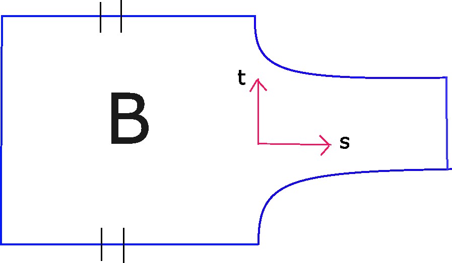
Figure 3: The open-closed surface

Let $Y_{\varphi_{H}}:=[0,2]\times\Sigma/(0,\varphi_{H}(x))\sim(2,x)$ be the mapping torus of $\varphi_{H}$. Then $\pi:\mathbb{R}_{s}\times Y_{\varphi_{H}}\to\mathbb{R}_{s}\times(\mathbb{R}_{t}/(2\mathbb{Z}))$ is a surface bundle over the cylinder. Define a surface bundle $W_{H}$ by

$$\pi_{W}=\pi|_{W}:W_{H}:=\pi^{-1}(B)\to B.$$

The symplectic form $\Omega_{H}$ on $W_{H}$ is defined to be the restriction of $\omega_{\varphi_{H}}+ds\wedge dt$. Note that $W_{H}$ is diffeomorphic (preserving the fibration structure) to the $B\times\Sigma$. So we denote $W_{H}$ by $W$ instead when the context is clear.

We place a copy of $\underline{L}$ on the fiber $\pi_{W}^{-1}(3,1)$ and take its parallel transport along $\partial B$ using the symplectic connection. The parallel transport sweeps out an $\Omega_{H}$-Lagrangian submanifold $\mathcal{L}_{H}$ in $W$. Then $\mathcal{L}_{H}$ consists of $d$-disjoint connected components. Moreover, we have

$$\begin{split}&\mathcal{L}_{H}|_{s\geq 3\times\{0\}}=\mathbb{R}_{s\geq 3}\times\{0\}\times\varphi_{H}(\underline{L})\\ &\mathcal{L}_{H}|_{s\geq 3\times\{1\}}=\mathbb{R}_{s\geq 3}\times\{1\}\times\underline{L}.\end{split}$$

We call the triple $(W_{H},\Omega_{H},\mathcal{L}_{H})$ an open-closed cobordism.

Definition 5.1 (Definition 5.4.3 of [15]).

Fix a Reeb chord $\mathbf{y}$ and an orbit set $\gamma$ with degree $d$. Let $(\dot{F},j)$ be a Riemann surface (possibly disconnected) with punctures. A d–multisection in $W$ is a smooth map $u:(\dot{F},\partial\dot{F})\to W$ such that

1. $u(\partial{\dot{F}})\subset\mathcal{L}_{H}$. Write $\mathcal{L}_{H}=\cup_{i=1}^{d}L^{i}_{H}$, where $L_{H}^{i}$ is a connected component of $\mathcal{L}_{H}$. For each $1\leq i\leq d$, $u^{-1}(L_{H}^{i})$ consists of exactly one component of $\partial\dot{F}$.

2. $u$ is asymptotic to $\mathbf{y}$ as $s\to\infty$.

3. $u$ is asymptotic to $\gamma$ as $s\to-\infty$.

4. $\int_{F}u^{*}\omega_{\varphi_{H}}<\infty$.

A $J$-holomorphic $d$-multisection is called an HF-PFH curve. We remark that the HF-PFH curves are simple because they are asymptotic to Reeb chords. This observation is crucial in the proof of Theorem 2.

Let

$$Z_{\textbf{y},\gamma}:=\mathcal{L}_{H}\cup(\{\infty\}\times\textbf{y})\cup(\{-\infty\}\times\gamma)\subset W.$$

We denote $H_{2}(W,\textbf{y},\gamma)$ the equivalence classes of continuous maps $u:(\dot{F},\partial\dot{F})\to(W,Z_{\textbf{y},\gamma})$ satisfying 1), 2), 3) in the above definition. Two maps are equivalent if they represent the same element in $H_{2}(W,Z_{\textbf{y},\gamma};\mathbb{Z})$. Note that $H_{2}(W,\textbf{y},\gamma)$ is an affine space of $H_{2}(W,\mathcal{L}_{H};\mathbb{Z})$. The difference of any two classes can be written as

$$\mathcal{Z}^{\prime}-\mathcal{Z}=\sum_{i=1}^{k}c_{i}[B_{i}]+m[\Sigma]+[S],$$

where $[B_{i}]$ is the class represented by the parallel translation of $B_{i}$ and $[S]$ is a class in the $H_{1}(S^{1},\mathbb{Z})\otimes H_{1}(\Sigma,\mathbb{Z})$-component of $H_{2}(Y_{\varphi_{H}},\mathbb{Z})$.

Fix a nonvanishing vector field on $\underline{L}$. This gives a trivialization $\tau$ of $T\Sigma|_{\underline{L}}$. We extend it to $T\Sigma|_{\mathcal{L}_{H}}$ by using the symplectic parallel transport. We then extend the trivialization of $T\Sigma|_{\mathcal{L}_{H}}$ in an arbitrary manner along $\{\infty\}\times\textbf{y}$ and along $\{-\infty\}\times\gamma$. Then we can define the relative Chern number $c_{1}(u^{*}T\Sigma,\tau)$. This is the obstruction of extending $\tau$ to $u$.

Define a real line bundle $\mathfrak{L}$ of $T\Sigma$ along $\mathcal{L}_{H}\cup\{\infty\}\times\textbf{y}$ as follows. We set $\mathfrak{L}|_{\mathcal{L}_{H}}:=T\mathcal{L}_{H}\cap T\Sigma$. Then extend $\mathfrak{L}$ across $\{\infty\}\times\textbf{y}$ by rotating in the counterclockwise direction from $T\varphi_{H}(\underline{L})$ to $T\underline{L}$ in $T\Sigma$ by the minimum amount. With respect to the trivialization $\tau$, we have Maslov index for the bundle pair $(u^{*}\mathfrak{L},u^{*}T\Sigma)$, denoted by $\mu_{\tau}(u)$.

The Fredholm index for an HF-PFH curve is

$$\begin{split}indu:=-\chi(\dot{F})-d+2c_{1}(u^{*}T\Sigma,\tau)+\mu_{\tau}(u)-\mu^{ind}_{\tau}(\gamma).\end{split}$$

The notation $\mu^{ind}_{\tau}(\gamma)$ is explained as follows. Let $\gamma=\{(\gamma_{i},m_{i})\}$. Suppose that for each $i$, $u$ has $k_{i}$-negative ends and each end is asymptotic to $\gamma_{i}^{q_{j}}$. Then the total multiplicity is $m_{i}=\sum_{j=1}^{k_{i}}q_{j}$. Define

$$\mu^{ind}_{\tau}(\gamma):=\sum_{i}\sum_{j=1}^{k_{i}}CZ_{\tau}(\gamma_{i}^{q_{j}}),$$

where $CZ_{\tau}$ is the Conley-Zehnder index.

Given $\mathcal{Z}\in H_{2}(W,\textbf{y},\gamma)$, the ECH index is (see Definition 5.6.5 of [15])

$$\begin{split}I(\mathcal{Z}):=c_{1}(TW|_{\mathcal{Z}},\tau)+Q_{\tau}(\mathcal{Z})+\mu_{\tau}(\mathcal{Z})-\mu^{ech}_{\tau}(\gamma)-d,\end{split}$$

where $\mu^{ech}(\gamma):=\sum_{i}\sum_{p=1}^{m_{i}}CZ_{\tau}(\gamma_{i}^{p})$.

We define the $J_{0}$ index of $\mathcal{Z}$ by

$$\begin{split}J_{0}(\mathcal{Z}):=-c_{1}(TW|_{\mathcal{Z}},\tau)+Q_{\tau}(\mathcal{Z})-\mu^{J_{0}}_{\tau}(\gamma),\end{split}$$

where $\mu^{J_{0}}_{\tau}(\gamma)=\sum_{i}\sum_{p=1}^{m_{i}-1}\mu_{\tau}(\gamma^{p})$.

The index inequalities still hold in the open-closed setting.

Theorem 5.2.

(Theorem 5.6.9 of [15], Lemma 5.2 of [13]) Let $u\in\mathcal{M}^{J}(\mathbf{y},\gamma)$ be an irreducible HF-PFH curve in $(W_{H},\Omega_{H},\mathcal{L}_{H})$. Then we have

$$\begin{split}&I(u)\geq indu+2\delta(u)\\ &J_{0}(u)\geq 2(g(F)-1+\delta(u))+\#\partial F+|\gamma|,\end{split}$$

where $|\gamma|$ is a quantity satisfying $|\gamma|\geq 1$ provided that it is nonempty. Moreover, $I(u)=indu$ holds if and only if $u$ satisfies the ECH partition condition. If $u=\cup_{a}u_{a}$ is an HF-PFH curve consisting of several (distinct) irreducible components, then

$$\begin{split}&I(u)\geq\sum_{a}I(u_{a})+\sum_{a\neq b}2\#(u_{a}\cap u_{b}),\\ &J_{0}(u)\geq\sum_{a}J_{0}(u_{a})+\sum_{a\neq b}2\#(u_{a}\cap u_{b}).\end{split}$$

In particular, $J_{0}(u)\geq 0$ for an HF-PFH curve.

In this paper, we don’t need the details on “ECH partition condition” and $|\gamma|$. For the readers who are interested in it, please refer to [18, 19]. The proof of Theorem 5.2 basically is a combination of the relative adjunction formula and Hutchings’s analysis in [19]. We omit the details here.

5.1 Construction and invariance of $\mathcal{OC}$

In this subsection, we outline the construction of the open-closed morphisms. Also, we will explain why it satisfies the partial invariance.

To begin with, we need the following lemma to rule out the bubbles.

Lemma 5.3.

Let $\mathcal{Z},\mathcal{Z}\in H_{2}(W,\mathbf{y},\gamma)$ be relative homology classes such that $\mathcal{Z}^{\prime}-\mathcal{Z}=m[\Sigma]+\sum_{i=1}^{k}c_{i}[B_{i}]+[S]$, where $[S]\in H_{1}(S^{1},\mathbb{Z})\otimes H_{1}(\Sigma,\mathbb{Z})$. Then we have

$$\begin{split}&I(\mathcal{Z}^{\prime})=I(\mathcal{Z})+\sum_{i}^{k}2c_{i}+2m(k+1)\\ &J_{0}(\mathcal{Z}^{\prime})=J_{0}(\mathcal{Z})+2m(d+g-1).\end{split}$$ (5.31)

Proof.

Using the same argument in Lemma 3.3 of [13], we know that adding $B_{i}$ to a relative homology class $\mathcal{Z}$ will increase the ECH index by 2 because the Maslov index of $B_{i}$ is 2. Also, the adding disks will not change the topology of the curves. Hence, $J_{0}$ is still the same.

If we add $[\Sigma]$ to $\mathcal{Z}$, then the ECH index will increase by $2(k+1)$. See the index ambiguity formula in Proposition 1.6 of [18]. Similarly, adding $[S]$ doesn’t change the ECH index and $J_{0}$ index. ∎

Fix a reference relative homology class $\mathcal{Z}_{ref}\in H_{2}(W,\textbf{x}_{H},\gamma_{ref})$. The open-closed morphism in chain level is defined by

$$\mathcal{OC}_{\mathcal{Z}_{ref}}(W_{H},\Omega_{H},\mathcal{L}_{H})_{J}(\textbf{y},[A])=\sum_{(\gamma,[Z])}\sum_{\mathcal{Z},I(\mathcal{Z})=0}\#\mathcal{M}^{J}(\textbf{y},\gamma,\mathcal{Z})(\gamma,[Z]),$$

The class $Z$ is characterized by $A\#\mathcal{Z}\#Z=\mathcal{Z}_{ref}.$ The arguments in [15] (also see the relevant argument for closed-open morphisms [13]) show that this is well defined and it is a chain map. The main difference here with [15] is that the bubbles would appear, but these can be ruled out by Lemma 5.3 and the argument in Proposition 3.5.

To prove the partial invariance, the arguments consist of the following key steps:

1. If we deform the open-closed morphism smoothly over a compact set of $W$ (the deformation needs to be generic), then the standard homotopy arguments show that the open-closed morphism is invariant.

2. Assume that $\varphi_{H}$ satisfies $\spadesuit$.1 and $\varphi_{G}$ satisfies $\spadesuit$.2. Let $(E_{1},\Omega_{1},\mathcal{L}_{1})$ be a Lagrangian cobordism from $(\varphi_{G}(\underline{L}),\underline{L})$ to $(\varphi_{H}(\underline{L}),\underline{L})$. Let $(X,\Omega_{X})$ be a symplectic cobordism from $(Y_{\varphi_{H}},\omega_{\varphi_{H}})$ to $(Y_{\varphi_{G}},\omega_{\varphi_{G}})$ defined by (2.9). Consider the $R$-stretched composition of $(E_{1},\Omega_{1},\mathcal{L}_{1})$, $(W_{H},\Omega_{H},\mathcal{L}_{H})$ and $(X,\Omega_{X})$, denoted by $(W_{R},\Omega_{R},\mathcal{L}_{R})$. As $R\to\infty$, the $I=0$ HF-PFH curves in $(W_{R},\Omega_{R},\mathcal{L}_{R})$ converges to a holomorphic building. Under assumptions $\spadesuit$.1, $\spadesuit$.2, the holomorphic curves in $(X,\Omega_{X})$ have nonnegative ECH index (see Section 7.1 of [11]). Combining this with Theorems 3.3, 5.2, the holomorphic curves in each level have nonnegative ECH index. As a result, these holomorphic curves have zero ECH index. They are either embedded or branched covers of trivial cylinders. By Huctings-Taubes’s gluing argument [24, 25], the open-closed morphism defined by $(W_{R},\Omega_{R},\mathcal{L}_{R})$ is equal to $I^{G,H}_{0,0}\circ(\mathcal{OC}_{\mathcal{Z}_{ref}}(W_{H},\Omega_{H},\mathcal{L}_{H}))_{*}\circ PFH_{Z_{ref}}^{hol}(X,\Omega_{X})$ for $R\gg 1$. Here $PFH_{Z_{ref}}^{hol}(X,\Omega_{X})$ is the PFH cobordism map defined by counting embedded holomorphic curves in $X$. By Theorem 3 in [11], we can replace it by $PFH_{Z_{ref}}^{sw}(X,\Omega_{X})$. Finally, by the homotopy invariance in step 1, we get the partial invariance.

For more details, we refer the readers to [13].

5.2 Computations of $\mathcal{OC}$

In this subsection, we compute the open-closed morphism for a special Hamiltonian function $H$ satisfying $\spadesuit$.1. Using partial invariance, we deduce the non-vanishing result under the assumption $\spadesuit$.2. The main idea here is also the same as [13].

Suppose that $f$ is a Morse function satisfying M.1, M.2, M.3, and M.4. Define $H_{\epsilon}=-\epsilon f$, where $0<\epsilon\ll 1$. $H_{\epsilon}$ is a slight perturbation of the height function in Figure 1. This is a nice candidate for computation because we can describe the periodic orbits and Reeb chords in terms of the critical points and the index of holomorphic curves are computable. However, the $H_{\epsilon}$ doesn’t satisfy $\spadesuit$.1 or $\spadesuit$.2. We need to follow the discussion in Section 6.1 of [13] to modify $H_{\epsilon}$.

Fix numbers $0<\epsilon_{0}\ll 1$ and $\delta,\delta_{0}>0$. By [13], we have a function $\varepsilon:\Sigma\to\mathbb{R}$ such that $0<\epsilon\leq\varepsilon\leq\epsilon_{0}$ and the new autonomous Hamiltonian function $H_{\varepsilon}=-\varepsilon f$ satisfies the following conditions:

1. There is an open set $\mathcal{U}^{\delta+\delta_{0}}=\cup_{p}U^{\delta+\delta_{0}}_{p}$ such that $H_{\varepsilon}|_{\Sigma-\mathcal{U}^{\delta+\delta_{0}}}=H_{\epsilon}|_{\Sigma-\mathcal{U}^{\delta+\delta_{0}}}$, where $p$ runs over all the local maximums of $-f$ and $U^{\delta+\delta_{0}}_{p}$ is a $(\delta+\delta_{0})$-neighbourhood of $p$.

2. $H_{\varepsilon}$ is still a Morse function satisfying the Morse-Smale conditions. Moreover, $Crit(H_{\varepsilon})=Crit(-f)$.

3. $\varphi_{H_{\varepsilon}}$ is $d$-nondegenerate. The periodic orbits of $\varphi_{H_{\varepsilon}}$ with period at most $d$ are covers of the constant orbits at critical points of $H_{\varepsilon}$.

4. For each local maximum $p$, $\varphi_{H_{\varepsilon}}$ has a family periodic orbits $\gamma_{r_{0},\theta}(t)$ that foliates $S_{t}^{1}\times\partial\mathcal{U}^{r_{0}}_{p}$, where $\delta+\delta_{0}\leq r_{0}\leq\delta+2\delta_{0}$. Moreover, the period of $\gamma_{r_{0},\theta}(t)$ is strictly greater than $d$.

5. The Reeb chords of $\varphi_{H_{\varepsilon}}$ are still corresponding to the critical points of $\cup_{i=1}^{d}f_{L_{i}}$. See (3.22).

By Proposition 3.7 of [11], we perturb $H_{\varepsilon}$ to a new Hamiltonian function $H_{\varepsilon}^{\prime}$ (may depend on $t$) such that it satisfies the following properties:

1. $H^{\prime}_{\varepsilon}|_{\Sigma-\mathcal{U}^{\delta}}=H_{\varepsilon}|_{\Sigma-\mathcal{U}^{\delta}}$.

2. $H_{\varepsilon}^{\prime}$ still satisfies F.4 and F.5.

3. $|H_{\varepsilon}^{\prime}-H_{\varepsilon}|\leq c_{0}\delta$ and $|dH_{\varepsilon}^{\prime}-dH_{\varepsilon}|\leq c_{0}\delta$.

4. The periodic orbits of $\varphi_{H^{\prime}_{\varepsilon}}$ with period less than or equal to $d$ are either hyperbolic or $d$-negative elliptic. In other words, $\varphi_{H^{\prime}_{\varepsilon}}$ is $d$-nondegenerate and satisfies $\spadesuit$.1.

Remark 5.1.

Because we take $H_{\varepsilon}=-\varepsilon f$, the maximum points $\{y_{i}^{+}\}$ of $f$ are the minimum points of $H_{\varepsilon}$. We use $\{y_{-}^{i}\}$ to denote the minimum points of $H_{\varepsilon}$ from now on.

Let $y$ be a critical point of $H_{\varepsilon}$. Let $\gamma_{y}$ denote the constant simple periodic orbit at the critical point $y$. We define PFH generators and a Reeb chord as follows:

1. Let $I=(i_{1},...i_{d})$. Here we allow $i_{j}=i_{k}$ for $j\neq k$. Let $\alpha_{I}=\gamma_{y_{-}^{i_{1}}}...\gamma_{y_{-}^{i_{d}}}$. When $I=(1,2...,d)$, we denote $\alpha_{I}$ by $\alpha_{\diamondsuit}$. Here we use multiplicative notation to denote an orbit set instead.

2. $\textbf{y}_{\diamondsuit}=[0,1]\times(y_{-}^{1},...y_{-}^{d})$.

Let $\alpha=\gamma_{p_{1}}\cdots\gamma_{p_{d}}$ and $\beta=\gamma_{q_{1}}\cdots\gamma_{q_{d}}$ be two orbit sets, where $p_{i},q_{j}\in Crit(H_{\varepsilon})$. Following [13], we define a relative homology class $Z_{\alpha,\beta}$ as follows: Let $\eta=\sqcup_{i=1}^{d}\eta_{i}:\sqcup_{i=1}^{d}[0,1]\to\Sigma$ be a union of paths with $d$ components such that $\eta_{i}(1)=p_{i}$ and $\eta_{i}(0)=q_{i}$. Define a relative homology class

$$Z_{\alpha,\beta}:=[S^{1}\times\eta]\in H_{2}(Y_{\varphi_{H_{\varepsilon}}},\alpha,\beta).$$ (5.32)

We also use this way to define $Z_{\alpha}\in H_{2}(Y_{\varphi_{H_{\varepsilon}}},\alpha,\gamma_{H}^{\textbf{x}})$.

Let $\mathcal{J}(W,\Omega_{H^{\prime}_{\varepsilon}})\subset\mathcal{J}_{tame}(W,\Omega_{H^{\prime}_{\varepsilon}})$ be a set of almost complex structures which are the restriction of admissible almost complex structures in $\mathcal{J}(Y_{\varphi_{H^{\prime}_{\varepsilon}}},\omega_{\varphi_{H^{\prime}_{\varepsilon}}})$.

Take a $J\in\mathcal{J}(W,\Omega_{H^{\prime}_{\varepsilon}})$. Let $u_{y_{i}}$ be the restriction of $\mathbb{R}\times\gamma_{y_{i}}$ to $W$. Obviously, it is a $J$–holomorphic curve in $\mathcal{M}^{J}(y_{i},\gamma_{y_{i}})$. It is called a horizontal section of $(W,\Omega_{H_{\varepsilon}^{\prime}},\mathcal{L}_{{H^{\prime}_{\varepsilon}}},J)$. Moreover, it is easy to check that $indu_{y_{-}^{i}}=0$ from the definition.

Lemma 5.4.

Let $u:F\to W$ be a $J$–holomorphic HF-PFH curve in $(W,\Omega_{H},\mathcal{L}_{{H}})$ and $J\in\mathcal{J}(W,\Omega_{H})$. Then the $\omega_{\varphi_{H}}$-energy satisfies

$$E_{\omega_{\varphi_{H}}}(u):=\int_{F}u^{*}\omega_{\varphi_{H}}\geq 0.$$

Moreover, when $H=H^{\prime}_{\varepsilon}$, $E_{\omega_{\varphi_{H}}}(u)=0$ if and only if $u$ is a union of the horizontal sections.

Proof.

The proof is the same as Lemma 6.6 in [13]. ∎

The horizontal sections $\cup_{i=1}^{d}u_{y_{-}^{i}}$ represent a relative homology class $\mathcal{Z}_{hor}$. We take the reference relative homology class to be $\mathcal{Z}_{ref}=A_{\textbf{y}_{\diamondsuit}}\#\mathcal{Z}_{hor}\#Z_{\alpha_{\diamondsuit}}\in H_{2}(W,\textbf{x}_{H},\gamma_{H}^{\textbf{x}}).$

Lemma 5.5.

For a generic $J\in\mathcal{J}(W,\Omega_{H^{\prime}_{\varepsilon}})$, we have

$$\mathcal{OC}_{\mathcal{Z}_{ref}}(W,\Omega_{H^{\prime}_{\varepsilon}},\mathcal{L}_{H^{\prime}_{\varepsilon}})_{J}(\mathbf{y}_{\diamondsuit},A_{\mathbf{y}_{\diamondsuit}})=(\alpha_{\diamondsuit},Z_{\alpha_{\diamondsuit}})+\sum(\beta,Z),$$

Here $(\beta,Z)$ satisfies $\beta\neq\alpha_{\diamondsuit}$ and $\mathbb{A}^{\eta}_{H^{\prime}_{\varepsilon}}(\alpha_{\diamondsuit},Z_{\alpha_{\diamondsuit}})>\mathbb{A}^{\eta}_{H^{\prime}_{\varepsilon}}(\beta,Z)$.

Proof.

Consider the moduli space of HF-PFH curves $\mathcal{M}_{0}^{J}(\textbf{y}_{\diamondsuit},\alpha_{\diamondsuit})$ with $I=0$. Let $u\in\mathcal{M}_{0}^{J}(\textbf{y}_{\diamondsuit},\alpha_{\diamondsuit})$. By Lemma 5.3, $J_{0}(u)=2m(d+g-1)$. Also, $I(u)=0$ implies that $\sum_{i=1}^{k}c_{i}+m(k+1)=0$.

On the other hand,

$$\begin{split}E_{\omega_{H^{\prime}_{\varepsilon}}}(u)+\eta J_{0}(u)&=\int|d^{vert}u|^{2}+\eta J_{0}(u)\\ &=\sum_{i=1}^{k}\lambda c_{i}+m+\eta 2m(d+g-1)=\lambda\left(\sum_{i=1}^{k}c_{i}+(k+1)m\right)=0.\end{split}$$

Theorem 5.2 and Lemma 5.4 imply that $u=\cup_{i}u_{y_{-}^{i}}$ is a union of horizontal sections. In other words, the union of horizontal sections is the unique element in $\mathcal{M}_{0}^{J}(\textbf{y}_{\diamondsuit},\alpha_{\diamondsuit})$.

If $u$ is an HF-PFH curve in $\mathcal{M}_{0}^{J}(\textbf{y}_{\diamondsuit},\beta)$ and $\beta\neq\alpha_{{\diamondsuit}}$, then $E_{\omega_{\varphi_{H^{\prime}_{\varepsilon}}}}(u)>0$; otherwise, $u$ is horizontal and $u$ must be asymptotic to $\alpha_{{\diamondsuit}}$. By Theorem 5.2, we have

$$\begin{split}0<E_{\omega_{H^{\prime}_{\varepsilon}}}(u)+\eta J_{0}(u)&=\int_{\mathcal{Z}_{ref}}\omega_{\varphi_{H^{\prime}_{\varepsilon}}}-\int_{A_{\textbf{y}_{\diamondsuit}}}\omega-\int_{Z}\omega_{\varphi_{H^{\prime}_{\varepsilon}}}+\eta(J_{0}(\mathcal{Z}_{ref})-J_{0}(A_{\mathbf{y}_{\diamondsuit}})-J_{0}(Z))\\ &=\int_{Z_{\alpha_{\diamondsuit}}}\omega_{\varphi_{H^{\prime}_{\varepsilon}}}-\int_{Z}\omega_{\varphi_{H^{\prime}_{\varepsilon}}}+\eta(J_{0}(Z_{\alpha_{\diamondsuit}})-J_{0}(Z))\\ &=\mathbb{A}^{\eta}_{H^{\prime}_{\varepsilon}}(\alpha_{\diamondsuit},Z_{\alpha_{\diamondsuit}})-\mathbb{A}^{\eta}_{H^{\prime}_{\varepsilon}}(\beta,Z).\end{split}$$

∎

The following lemma tells us that $(\textbf{y}_{\diamondsuit},A_{\textbf{y}_{\diamondsuit}})$ is a cycle.

Lemma 5.6.

Let $d_{J}$ be the differential of $CF(\Sigma,\varphi_{H^{\prime}_{\varepsilon}}(\underline{L}),\underline{L})$. Then $d_{J}=0$. In particular, $(\mathbf{y}_{\diamondsuit},A_{\mathbf{y}_{\diamondsuit}})$ is a cycle.

Proof.

By F.5, we know that $CF(\Sigma,\varphi_{H^{\prime}_{\varepsilon}}(\underline{L}),\underline{L})\cong\oplus^{2^{d}}R$. According to Lemma 6.8 in [7], we know that

$$CF(\Sigma,\varphi_{H^{\prime}_{\varepsilon}}(\underline{L}),\underline{L})\cong H^{*}(\mathbb{T}^{d},R)\cong HF(\Sigma,\varphi_{H^{\prime}_{\varepsilon}}(\underline{L}),\underline{L})$$

as vector spaces. Since $dim_{R}HF(\Sigma,\varphi_{H^{\prime}_{\varepsilon}}(\underline{L}),\underline{L})\leq dim_{R}\ker d_{J}\leq dim_{R}CF(\Sigma,\varphi_{H^{\prime}_{\varepsilon}}(\underline{L}),\underline{L})$, we must have $d_{J}=0$. ∎

Let $\mathfrak{c}:=\mathcal{OC}_{\mathcal{Z}_{ref}}(W,\Omega_{\varphi_{H^{\prime}_{\varepsilon}}},\mathcal{L}_{\omega_{\varphi_{H^{\prime}_{\varepsilon}}}})_{J}(\textbf{y}_{{{\diamondsuit}}},A_{\textbf{y}_{\diamondsuit}})$. By Lemma 5.6, $\mathfrak{c}$ is a cycle. To show that $\mathfrak{c}$ is non-exact, we first need to find the corresponding cycle $\mathfrak{c}^{\prime}\in\widetilde{PFC}(\Sigma,\varphi_{H_{\varepsilon}},\gamma_{0})$ because the elements in $\widetilde{PFC}(\Sigma,\varphi_{H_{\varepsilon}},\gamma_{0})$ can be figured out easily.

Let $(X,\Omega_{X})$ be the symplectic cobordism in (2.9). We take $H_{+}=H^{\prime}_{\varepsilon}$ and $H_{-}=H_{\varepsilon}.$ Note that $\Omega_{X}=\omega+dH_{\varepsilon}\wedge dt+ds\wedge dt$ is $\mathbb{R}$-invariant over $\mathbb{R}\times S^{1}_{t}\times(\Sigma-\mathcal{U}^{\delta+\delta_{0}})$. This region is called a product region. Take $Z_{ref}=[\mathbb{R}\times S^{1}\times\mathbf{x}]\in H_{2}(X,\gamma_{H^{\prime}_{\varepsilon}}^{\mathbf{x}},\gamma_{H_{\varepsilon}}^{\mathbf{x}})$ be the reference homology class.

Let $\mathcal{J}_{comp}(X,\Omega_{X})$ be the set of $\Omega_{X}$-compatible almost complex structures such that

1. $J_{X}|_{s\geq R_{0}}\in\mathcal{J}(Y_{\varphi_{H^{\prime}_{\varepsilon}}},\omega_{\varphi_{H^{\prime}_{\varepsilon}}})$ and $J_{X}|_{s\leq 0}\in\mathcal{J}(Y_{\varphi_{H_{\varepsilon}}},,\omega_{\varphi_{H_{\varepsilon}}})$.

2. $j\circ\pi_{*}=\pi_{*}\circ J_{X}$, where $j$ is the complex structure on $\mathbb{R}_{s}\times S^{1}_{t}$ that $j(\partial_{s})=\partial_{t}$.

In the following lemmas, we compute $PFC_{Z_{ref}}^{sw}(X,\Omega_{X})_{J_{X}}(\mathfrak{c}).$

Lemma 5.7.

Let $J_{X}\in\mathcal{J}_{comp}(X,\Omega_{X})$ be an almost complex structure such that it is $\mathbb{R}$-invariant in the product region $\mathbb{R}\times S^{1}_{t}\times(\Sigma-\mathcal{U}^{\delta+\delta_{0}})$. Let $\overline{\mathcal{M}_{0}^{J_{X}}(\alpha_{{\diamondsuit}},\alpha_{I})}$ be the moduli space of broken holomorphic curves with $I=0$. Then $\overline{\mathcal{M}_{0}^{J_{X}}(\alpha_{{\diamondsuit}},\alpha_{I})}=\emptyset$ unless $\alpha_{I}=\alpha_{\diamondsuit}$. In the case that $\alpha_{I}=\alpha_{\diamondsuit}$, the trivial cylinder is the unique element in $\overline{\mathcal{M}_{0}^{J_{X}}(\alpha_{\diamondsuit},\alpha_{\diamondsuit})}$.

Proof.

Let $\mathcal{C}\in\overline{\mathcal{M}_{0}^{J_{X}}(\alpha_{\diamondsuit},\alpha_{I})}$ be a (broken) holomorphic curve. Let $Z\in H_{2}(X,\alpha_{\diamondsuit},\alpha_{I})$ denote the relative homology class of $\mathcal{C}$. Then $Z$ can be written as $Z_{\alpha_{\diamondsuit},\alpha_{I}}+m(Z)[\Sigma]+[S]$, where $[S]\in H_{1}(S^{1},\mathbb{Z})\otimes H_{1}(\Sigma,\mathbb{Z})$. It is easy to show that

$$\begin{split}&I(\alpha_{\diamondsuit},\alpha_{I},Z)=2m(Z)(k+1)\mbox{ and }\int_{Z}\omega_{X}=m(Z).\end{split}$$

Then $m(Z)=0$ because $I=0$. Also, we have

$$\begin{split}\#(\mathcal{C}\cap\mathbb{R}\times\gamma_{r_{0},\theta})=\#((Z_{\alpha_{\diamondsuit},\alpha_{I}}+[S])\cap\mathbb{R}\times\gamma_{r_{0},\theta})=0.\end{split}$$

Note that the above intersection numbers are well defined because $\gamma_{r_{0},\theta}$ and $\alpha_{I}$ are disjoint. Because $\mathbb{R}\times\gamma_{r_{0},\theta}$ is holomorphic by the choice of $J_{X}$, the above equality implies that $\mathcal{C}$ doesn’t intersect $\mathbb{R}\times\gamma_{r_{0},\theta}$. In particular, $\mathcal{C}$ is contained in the product region $\mathbb{R}\times S^{1}_{t}\times(\Sigma-\mathcal{U}^{\delta+\delta_{0}})$. Then $\int_{\mathcal{C}}\omega_{X}=0$ implies that $\mathcal{C}$ is a union of trivial cylinders (Proposition 9.1 of [18]). Thus we must have $\alpha_{I}=\alpha_{\diamondsuit}$. ∎

Lemma 5.8.

Let $J_{X}$ be a generic almost complex structure in $\mathcal{J}_{comp}(X,\Omega_{X})$ and $J_{X}$ is $\mathbb{R}$-invariant in the product region $\mathbb{R}\times S^{1}_{t}\times(\Sigma-\mathcal{U}^{\delta+\delta_{0}})$. Then we have

$$PFC_{Z_{ref}}^{sw}(X,\Omega_{X})_{J_{X}}(\alpha_{\diamondsuit},Z_{\alpha_{\diamondsuit}})=(\alpha_{\diamondsuit},Z_{\alpha_{\diamondsuit}})+\sum(\beta^{\prime},Z^{\prime}),$$

where $(\beta^{\prime},Z^{\prime})$ satisfies $\mathbb{A}_{H^{\prime}_{\varepsilon}}(\alpha_{\diamondsuit},Z_{\alpha_{\diamondsuit}})-\mathbb{A}_{H_{\varepsilon}}(\beta^{\prime},Z^{\prime})\geq\frac{1}{4(k+1)}$ and $\beta^{\prime}\neq\alpha_{I}$.

Proof.

By the holomorphic axioms (Theorem 1 of [11] and Appendix of [13]) and Lemma 5.7, we know that

$$<PFC_{Z_{ref}}^{sw}(X,\Omega_{X})_{J_{X}}(\alpha_{\diamondsuit},Z_{\alpha_{\diamondsuit}}),(\alpha_{I},Z)>=0$$

when $(\alpha_{I},Z)\neq(\alpha_{\diamondsuit},Z_{\alpha_{\diamondsuit}})$, and

$$<PFC_{Z_{ref}}^{sw}(X,\Omega_{X})_{J_{X}}(\alpha_{\diamondsuit},Z_{\alpha_{\diamondsuit}}),(\alpha_{\diamondsuit},Z_{\alpha_{\diamondsuit}})>=1.$$

Assume that $<PFC_{Z_{ref}}^{sw}(X,\Omega_{X})_{J_{X}}(\alpha_{\diamondsuit},Z_{\alpha_{\diamondsuit}}),(\beta^{\prime},Z^{\prime})>=1$ for some $(\beta^{\prime},Z^{\prime})$ and $\beta^{\prime}\neq\alpha_{I}$. Again by the holomorphic axioms, we have a holomorphic curve $\mathcal{C}\in\overline{\mathcal{M}_{0}^{J}(\alpha_{\diamondsuit},\beta^{\prime})}$.

It is easy to check that

$$\begin{split}&I(\mathcal{C})=-h(\beta^{\prime})-2e_{+}(\beta^{\prime})+2m(k+1)=0\\ &\mathbb{A}_{H^{\prime}_{\varepsilon}}(\alpha_{\diamondsuit},Z_{\alpha_{\diamondsuit}})-\mathbb{A}_{H_{\varepsilon}}(\beta^{\prime},Z)=-H_{\varepsilon}(\beta^{\prime})+m,\end{split}$$ (5.33)

where $h(\beta^{\prime})$ is the total multiplicities of all the hyperbolic orbits in $\beta^{\prime}$ and $e_{+}(\beta^{\prime})$ is the total multiplicities of all the elliptic orbits at local maximum of $H_{\varepsilon}$.

Because $\beta^{\prime}\neq\alpha_{I}$, we have $h(\beta^{\prime})+2e_{+}(\beta^{\prime})\geq 1$. Therefore, we have

$$\begin{split}&\mathbb{A}_{H_{\varepsilon}}(\alpha_{\diamondsuit},Z_{\alpha_{\diamondsuit}})-\mathbb{A}_{H_{\varepsilon}}(\beta^{\prime},Z^{\prime})=-H_{\varepsilon}(\beta^{\prime})+\frac{h(\beta^{\prime})+2e_{+}(\beta^{\prime})}{2(k+1)}\geq\frac{1}{2(k+1)}+O(d\epsilon_{0})\geq\frac{1}{4(k+1)}.\end{split}$$

∎

Lemma 5.9.

Let $(\beta,Z)$ be a factor of $\mathfrak{c}$ given in Lemma 5.5. Let $J_{X}$ be the almost complex structure in Lemma 5.8. Then we have

$$PFC_{Z_{ref}}^{sw}(X,\Omega_{X})_{J_{X}}(\beta,Z)=\sum(\beta^{\prime},Z^{\prime}),$$

where $(\beta^{\prime},Z^{\prime})$ satisfies $\mathbb{A}^{\eta}_{H_{\varepsilon}}(\alpha_{\diamondsuit},Z_{\alpha_{\diamondsuit}})-\mathbb{A}^{\eta}_{H_{\varepsilon}}(\beta^{\prime},Z^{\prime})>0$ and $\beta^{\prime}\neq\alpha_{I}$.

Proof.

First, we show that $\beta^{\prime}$ cannot be $\alpha_{I}$. Assume that

$$<PFC_{Z_{ref}}^{sw}(X,\Omega_{X})_{J_{X}}(\beta,Z),(\alpha_{I},Z^{\prime})>=1.$$

Then we have a broken holomorphic curve $\mathcal{C}=(C,\mathcal{C}_{0})$, where $C\in\mathcal{M}_{0}^{J}(\textbf{y}_{\diamondsuit},\beta)$ is an HF-PFH curve and $\mathcal{C}_{0}\in\overline{\mathcal{M}_{0}^{J_{X}}(\beta,\alpha_{I})}$. The holomorphic curve gives us a relative homology class $\mathcal{Z}\in H_{2}(W,\textbf{y}_{\diamondsuit},\alpha_{I})$.

Reintroduce the periodic orbits $\gamma^{i}_{r_{0},\theta_{0}}$ near the local maximums of $H_{\varepsilon}$. The superscript “$i$” indicates that the local maximum lies in the domain $\mathring{B}_{i}$, where $1\leq i\leq k+1$. In particular, $\gamma^{i}_{r_{0},\theta_{0}}$ lies in $S^{1}\times\mathring{B}_{i}$. Define a curve $v_{i}:=(\mathbb{R}\times\gamma_{r_{0},\theta_{0}}^{i})\cap W$. Note that it is $J$–holomorphic and $\partial v_{i}$ is disjoint from the Lagrangian $\mathcal{L}_{{H^{\prime}_{\varepsilon}}}$. Then for any relative homology class $\mathcal{Z}^{\prime}\in H_{2}(W,\textbf{y}_{\diamondsuit},\alpha_{I})$, we have a well–defined intersection number

$$n_{i}(\mathcal{Z}^{\prime}):=\#(\mathcal{Z}^{\prime}\cap v_{i}).$$

The relative homology class $\mathcal{Z}\in H_{2}(W,\textbf{y}_{\diamondsuit},\alpha_{I})$ can be written as $\mathcal{Z}=\mathcal{Z}_{hor}\#Z_{\alpha_{\diamondsuit},\alpha_{I}}+\sum_{i=1}^{k}c_{i}[B_{i}]+m[\Sigma]+[S]$, where $[S]\in H_{1}(S^{1},\mathbb{Z})\otimes H_{1}(\Sigma,\mathbb{Z})$ and $\mathcal{Z}_{hor}$ is the class represented by the union of horizontal sections. By (5.31), the ECH index of $\mathcal{Z}$ is

$$I(\mathcal{Z})=\sum_{i}2c_{i}+2m(k+1)=I(C)+I(\mathcal{C}_{0})=0.$$ (5.34)

Let $q_{i}$ denote the period of $\gamma^{i}_{r_{0},\theta_{0}}$. From the construction in [13], the period of $\gamma^{i}_{r_{0},\theta_{0}}$ is determined by the function $\varepsilon$. For a suitable choice of $\varepsilon$, we can choose $q_{i}=q$ for $1\leq i\leq k+1$. By definition, we have

$$n_{i}(\mathcal{Z}_{hor}\#Z_{\alpha_{\diamondsuit},\alpha_{I}})=0,\ \ n_{i}([B_{j}])=\delta_{ij}q\ \ n_{i}([S])=0\ \ \mbox{and }n_{i}([\Sigma])=q.$$ (5.35)

for $1\leq i,j\leq k+1$. From (5.34) and (5.35), we know that

$$\#(\mathcal{C}\cap(\sqcup_{i=1}^{k+1}v_{i}))=\sum_{i=1}^{k+1}n_{i}(\mathcal{Z})=\sum_{i=1}^{k}c_{i}q+(k+1)mq=0.$$

By the intersection positivity of holomorphic curves, $\mathcal{C}$ doesn’t intersect $\mathbb{R}\times\gamma^{i}_{r_{0},\theta_{0}}$. In particular, $\mathcal{C}_{0}$ lies inside the product region of $X$. Therefore, $\int_{\mathcal{C}_{0}}{\omega_{\varphi_{H^{\prime}_{\varepsilon}}}}\geq 0$ and $J_{0}(\mathcal{C}_{0})\geq 0$. By Theorem 5.2, $J_{0}(\mathcal{Z})=J_{0}(C)+J_{0}(\mathcal{C}_{0})\geq 0.$ By (5.34), Lemmas 5.3, 5.4, we have

$$\begin{split}\int_{\mathcal{Z}}\omega_{\varphi_{H^{\prime}_{\varepsilon}}}+\eta J_{0}(\mathcal{Z})&=\int_{\mathcal{Z}_{hor}\#Z_{\alpha_{\diamondsuit},\alpha_{I}}}\omega_{\varphi_{H^{\prime}_{\varepsilon}}}+\lambda\sum_{i=1}^{k}c_{i}+m+2m\eta(d+g-1)\\ &=\lambda\left(\sum_{i=1}^{k}c_{i}+m(k+1)\right)=0,\\ \int_{\mathcal{Z}}\omega_{\varphi_{H^{\prime}_{\varepsilon}}}+\eta J_{0}(\mathcal{Z})&\geq\int_{C}{\omega_{\varphi_{H^{\prime}_{\varepsilon}}}}+\int_{\mathcal{C}_{0}}{\omega_{\varphi_{H^{\prime}_{\varepsilon}}}}>0.\end{split}$$

We obtain a contradiction.

Now we consider the case that $<PFC_{Z_{ref}}^{sw}(X,\Omega_{X})_{J_{X}}(\beta,Z),(\beta^{\prime},Z^{\prime})>=1$ and $\beta^{\prime}\neq\alpha_{I}.$ As before, we have a broken holomorphic curve $\mathcal{C}=(C,\mathcal{C}_{0})$, where $C\in\mathcal{M}_{0}^{J}(\textbf{y}_{\diamondsuit},\beta)$ is an HF-PFH curve and $\mathcal{C}_{0}\in\overline{\mathcal{M}^{J_{X}}(\beta,\beta^{\prime})}$.

Suppose that $\beta^{\prime}$ has $E_{+}$ distinct simple orbits (ignoring the multiplicity) at the local maximums and $E_{-}$ distinct simple orbits at the local minimums. Similar as (5.33), we have

$$\begin{split}&0=I(\mathcal{C})=I(C)+I(\mathcal{C}_{0})=-h(\beta^{\prime})-2e_{+}(\beta^{\prime})+\sum_{i=1}^{k}2c_{i}+2m(k+1)\\ &J_{0}(\mathcal{C})=d-h(\beta^{\prime})-2e_{+}(\beta^{\prime})+E_{+}-E_{-}+2m(d+g-1)\\ &\mathcal{A}_{H^{\prime}_{\varepsilon}}(\textbf{y}_{\diamondsuit},A_{\textbf{y}_{\diamondsuit}})-\mathbb{A}_{H_{\varepsilon}}(\beta^{\prime},Z^{\prime})=\int_{C}\omega_{\varphi_{H^{\prime}_{\varepsilon}}}+\int_{\mathcal{C}_{0}}\omega_{X}=-H_{\varepsilon}(\beta^{\prime})+m+\lambda\sum_{i=1}^{k}c_{i},\end{split}$$

where $h(\beta^{\prime})$ is the total multiplicities of the hyperbolic orbits and $e_{+}(\beta^{\prime})$ is the total multiplicities of the elliptic orbits at the local maximums. Note that $\mathcal{A}^{\eta}_{H^{\prime}_{\varepsilon}}(\textbf{y}_{\diamondsuit},[A_{\textbf{y}_{\diamondsuit}}])=\mathbb{A}^{\eta}_{H^{\prime}_{\varepsilon}}(\alpha_{\diamondsuit},Z_{\alpha_{\diamondsuit}})$. Therefore, we have

$$\begin{split}\mathbb{A}^{\eta}_{H^{\prime}_{\varepsilon}}(\alpha_{\diamondsuit},Z_{\alpha_{\diamondsuit}})-\mathbb{A}^{\eta}_{H_{\varepsilon}}(\beta^{\prime},Z^{\prime})&=-H_{\varepsilon}(\beta^{\prime})+m+\lambda\sum_{i=1}^{k}c_{i}+2m\eta(d+g-1)\\ &+\eta(d-h(\beta^{\prime})-2e_{+}(\beta^{\prime})+E_{+}-E_{-})\\ &\geq-H_{\varepsilon}(\beta^{\prime})+\lambda\sum_{i=1}^{k}c_{i}+\lambda m(k+1)-\eta(h(\beta^{\prime})+e_{+}(\beta^{\prime}))\\ &=-H_{\varepsilon}(\beta^{\prime})+(\frac{\lambda}{2}-\eta)(h(\beta^{\prime})+2e_{+}(\beta^{\prime})).\end{split}$$

Since $\beta^{\prime}\neq\alpha_{I}$, $h(\beta^{\prime})+2e_{+}(\beta^{\prime})\geq 1$. By assumption A.4, we have

$$\frac{\lambda}{2}-\eta=\frac{\lambda(2g-2)+1}{2(d+g-1)}.$$

If $g\geq 1$, then $\mathbb{A}^{\eta}_{H^{\prime}_{\varepsilon}}(\alpha_{\diamondsuit},Z_{\alpha_{\diamondsuit}})-\mathbb{A}^{\eta}_{H_{\varepsilon}}(\beta^{\prime},Z^{\prime})\geq-H_{\varepsilon}(\beta^{\prime})+\frac{1}{2(d+g-1)}>0.$ Recall that we assume $k>1$ (A.1). If $g=0$, then

$$\mathbb{A}^{\eta}_{H^{\prime}_{\varepsilon}}(\alpha_{\diamondsuit},Z_{\alpha_{\diamondsuit}})-\mathbb{A}^{\eta}_{H_{\varepsilon}}(\beta^{\prime},Z^{\prime})\geq-H_{\varepsilon}(\beta^{\prime})+\frac{k-2+2\int_{B_{k+1}}\omega}{2k(d+g-1)}>0.$$

∎

Lemma 5.10.

Let $\mathfrak{c}^{\prime}=PFC_{Z_{ref}}^{sw}(X,\Omega_{X})(\mathfrak{c})$. Then the cycle $\mathfrak{c}^{\prime}$ is non-exact, i.e., it represents a non-zero class in $\widetilde{PFH}(\Sigma,\varphi_{H_{\varepsilon}},\gamma_{{H_{\varepsilon}}}^{\mathbf{x}})$.

Proof.

Let $(X_{-},\Omega_{X_{-}})$ be the symplectic cobordism from $(Y_{\varphi_{H_{\varepsilon}}},\omega_{\varphi_{H_{\varepsilon}}})$ to $\emptyset$ in (2.10). Fix a generic $J_{X_{-}}\in\mathcal{J}_{comp}(X_{-},\Omega_{X_{-}})$. Using the same argument as in [12], we define a homomorphism

$$PFC^{hol}_{Z_{ref}}(X_{-},\Omega_{X_{-}})_{J_{X_{-}}}:\widetilde{PFC}(\Sigma,\omega_{\varphi_{H_{\varepsilon}}},\gamma_{{H_{\varepsilon}}}^{\mathbf{x}})\to\Lambda,$$

by counting $I=0$ (unbroken) holomorphic curves in $(X_{-},\Omega_{X_{-}})$. Moreover, this is a chain map. Therefore, $PFC^{hol}_{Z_{ref}}(X_{-},\Omega_{X_{-}})_{J_{X_{-}}}$ induces a homomorphism in homology level:

$$PFH^{hol}_{Z_{ref}}(X_{-},\Omega_{X_{-}})_{J_{X_{-}}}:\widetilde{PFH}(\Sigma,\omega_{\varphi_{H_{\varepsilon}}},\gamma_{{H_{\varepsilon}}}^{\mathbf{x}})\to\Lambda,$$

Using Taubes’s techniques [33, 34] and C. Gerig’s generalization [10], $PFH^{hol}_{Z_{ref}}(X_{-},\Omega_{X_{-}})_{J_{X_{-}}}$ should agree with the PFH cobordism map $PFH^{sw}_{Z_{ref}}(X_{-},\Omega_{X_{-}})_{J_{X_{-}}}$ (see Remark 1.3 of [12]). But we don’t need this to prove the lemma.

To show that $\mathfrak{c}^{\prime}$ is non-exact, it suffices to prove $PFC^{hol}_{Z_{ref}}(X_{-},\Omega_{X_{-}})_{J_{X_{-}}}(\mathfrak{c}^{\prime})\neq 0$. In [12], the author computes the map $PFC^{hol}_{Z_{ref}}(X,\Omega_{X})_{J_{X}}$ for the elementary Lefschetz fibration (a symplectic fibration over a disk with a single singularity). The current situation is an easier version of [12]. By the argument in [12], we have

$$\begin{split}&PFC^{hol}_{Z_{ref}}(X_{-},\Omega_{X_{-}})_{J_{X_{-}}}(\alpha_{I},Z_{I})=1,\\ &PFC^{hol}_{Z_{ref}}(X_{-},\Omega_{X_{-}})_{J_{X_{-}}}(\beta^{\prime},Z^{\prime})=0\mbox{ \ \ for $(\beta^{\prime},Z^{\prime})\neq(\alpha_{I},Z_{I})$}.\end{split}$$ (5.36)

Therefore, Lemmas 5.8 and 5.9 imply that $PFC^{hol}_{Z_{ref}}(X_{-},\Omega_{X_{-}})_{J_{X_{-}}}(\mathfrak{c}^{\prime})=1$.

Here let us explain a little more about how to get (5.36). Basically, the idea is the same as Lemma 3.8. From the computation of the ECH index, we know that $I=0$ implies that the holomorphic curves must be asymptotic to $\alpha_{I}$. Also, the energy is zero. Therefore, the unbranched covers of the horizontal sections are the only curves that contribute to $PFC^{hol}_{Z_{ref}}(X_{-},\Omega_{X_{-}})_{J_{X_{-}}}$, and this leads to (5.36). Even these holomorphic curves may not be simple, they are still regular (see [9]).

∎

6 Spectral invariants

In this section, we assume that the link $\underline{L}$ is $0$-admissible.

6.1 Comparing the PFH and HF spectral invariants

Let $H_{\varepsilon}$ be the function satisfying F.1, F.2, F.3, F.4, F.5 . Let $H_{\varepsilon}^{\prime}$ be the perturbation. Let $\textbf{y}_{\diamondsuit}=[0,1]\times(y_{-}^{1},..y_{-}^{d})$ be the Reeb chord of $\varphi_{H^{\prime}_{\varepsilon}}$, where $\{y_{-}^{i}\}_{i=1}^{d}$ are minimums of $H_{\varepsilon}$. By Lemma 5.6, $[(\textbf{y}_{\diamondsuit},[A_{\textbf{y}_{\diamondsuit}}])]$ represents a class $e_{\diamondsuit}\in HF(\Sigma,\underline{L})$, i.e., $e_{\diamondsuit}=j^{\mathbf{x}}_{H^{\prime}_{\varepsilon}}([(\textbf{y}_{\diamondsuit},[A_{\textbf{y}_{\diamondsuit}}])])$. Let $e$ be the unit of $HF(\Sigma,\underline{L})$. Reintroduce

$$\begin{split}c_{\underline{L}}^{+}(H):=c_{\underline{L},\eta=0}(H,e)\mbox{ and }c_{\underline{L}}^{-}(H):=c_{\underline{L},\eta=0}(H,e_{\diamondsuit}).\end{split}$$

Fix a base point $\textbf{x}=(x_{1},\cdots x_{d})$. Define a reference 1–cycle $\gamma_{H}^{\textbf{x}}:=\Psi_{H}(S^{1}\times\textbf{x})$. Let $(X,\Omega_{X})$ symplectic cobordism (2.8) from $(Y_{\varphi_{H}},\omega_{\varphi_{H}})$ to $(Y_{\varphi_{G}},\omega_{\varphi_{G}})$. Let $Z^{H,G}_{\textbf{x}}=[\mathbb{R}\times S^{1}\times\textbf{x}]\in H_{2}(X,\gamma_{H}^{\textbf{x}},\gamma_{G}^{\textbf{x}})$ be a reference class. Given another base point $\textbf{x}^{\prime}$, let $\eta$ be $d$ union of paths starting from x and ending at $\textbf{x}^{\prime}$. Let $Z_{\textbf{x}^{\prime},\textbf{x}}=[S^{1}\times\eta]\in H_{2}(X,\gamma_{H}^{\textbf{x}^{\prime}},\gamma_{H}^{\textbf{x}})$. The cobordism map $PFH^{sw}_{Z^{H,G}_{\mathbf{x}}}(X,\Omega_{X})$ only depends on $\mathbf{x},H,G$. Thus we denote it by $\mathfrak{I}^{\mathbf{x}}_{H,G}$.

The cycle $\mathfrak{c}=(\alpha_{\diamondsuit},Z_{\alpha_{{\diamondsuit}}})+\sum(\beta,Z)$ in Lemma 5.5 represents a class $\sigma_{{\diamondsuit}}\neq 0\in\widetilde{PFH}(\Sigma,\varphi_{H^{\prime}_{\varepsilon}},\gamma_{H^{\prime}_{\varepsilon}})$. Define

$$\begin{split}\sigma_{{\diamondsuit}H}^{\mathbf{x}}:=\Psi_{Z_{\mathbf{y}_{\diamondsuit},\mathbf{x}}}\circ\mathfrak{I}^{\mathbf{y}_{\diamondsuit}}_{H^{\prime}_{\varepsilon},H}(\sigma_{{\diamondsuit}}).\end{split}$$

Let $H_{-}$ and $H_{+}$ be Hamiltonian functions satisfying conditions $\spadesuit$.1 and $\spadesuit$.2 respectively. Let $W_{+}$ be the open-closed cobordism and $W_{-}$ the closed-open cobordism. Then by [13] and Theorem 2, we have

$$\begin{split}&\mathcal{CO}_{\mathcal{Z}^{-}_{ref}}(W_{-},\varphi_{H_{-}},\mathcal{L}_{H_{-}})_{*}(\sigma^{\mathbf{x}}_{\heartsuit H_{-}})=({j}_{H_{-}}^{\mathbf{x}})^{-1}(e)\\ &\mathcal{OC}_{\mathcal{Z}^{+}_{ref}}(W_{+},\Omega_{H_{+}},\mathcal{L}_{H_{+}})_{*}((j_{H_{+}}^{\mathbf{x}})^{-1}(e_{\diamondsuit}))=\sigma_{{\diamondsuit}H_{+}}^{\mathbf{x}}.\end{split}$$

Proof of Corollary 1.2.

The inequality $c_{\underline{L}}^{+}(H)\leq c^{pfh}_{d}(H,\sigma^{\mathbf{x}}_{\heartsuit H},\gamma^{\textbf{x}}_{H})+\int_{0}^{1}H_{t}(\textbf{x})dt$ is the Corollary 1.1 of [13].

To prove $c^{pfh}_{d}(H,\sigma^{\mathbf{x}}_{\diamondsuit H},\gamma^{\textbf{x}}_{H})+\int_{0}^{1}H_{t}(\mathbf{x})dt\leq c_{\underline{L}}^{-}(H)$, it suffices to prove the inequality for a Hamiltonian function $H$ satisfying $\spadesuit$.2 because of the Hofer-Lipschitz property and Remark 1.3. By using Theorem 2 and the argument in Section 7 of [13], we obtain the inequality.

By definition, $(\mathbf{y}_{\diamondsuit},A_{\mathbf{y}_{\diamondsuit}})$ represents $(j^{\mathbf{x}}_{H^{\prime}_{\varepsilon}})^{-1}(e_{\diamondsuit})=(j^{\mathbf{x}}_{-\epsilon f})^{-1}(e_{\diamondsuit}).$ Therefore,

$$c_{\underline{L}}(-\epsilon f,e_{\diamondsuit})\leq\mathcal{A}_{-\epsilon f}(\mathbf{y}_{\diamondsuit},A_{\mathbf{y}_{\diamondsuit}})=O(\epsilon).$$

Let $\epsilon\to 0$. We have $c_{\underline{L}}(0,e_{\diamondsuit})\leq 0$. By the triangle inequality, we have

$$\begin{split}c^{-}_{\underline{L}}(H)\leq c_{\underline{L}}^{+}(H)+c_{\underline{L}}(0,e_{\diamondsuit})\leq c_{\underline{L}}^{+}(H).\end{split}$$

∎

6.2 Homogenized spectral invariants

Let $\widetilde{Ham}(\Sigma,\omega)$ be the universal cover of ${Ham}(\Sigma,\omega)$. A element in $\widetilde{Ham}(\Sigma,\omega)$ is a homotopy class of paths $\{\varphi_{t}\}_{t\in[0,1]}\subset Ham(\Sigma,\omega)$ with fixed endpoints $\varphi_{0}=id$ and $\varphi_{1}=\varphi$. Let $\tilde{\varphi}\in\widetilde{Ham}(\Sigma,\omega)$ be a class represented by a path generated by a mean-normalized Hamiltonian $H$. Define

$$c_{\underline{L}}(\tilde{\varphi},a):=c_{\underline{L}}(H,a).$$

By Theorem 1, this is well defined. Thus, the HF spectral invariants descend to invariants on $\tilde{\varphi}\in\widetilde{Ham}(\Sigma,\omega)$. But in general, the spectral invariants cannot descend to ${Ham}(\Sigma,\omega)$. This is also true for PFH spectral invariants. To obtain numerical invariants for the elements in $Ham(\Sigma,\omega)$ rather than its universal cover, we need the homogenized spectral invariants. It is well known that $\widetilde{Ham}(\Sigma,\omega)=Ham(\Sigma,\omega)$ when $g(\Sigma)\geq 1$. Therefore, we only consider the case that $\Sigma=\mathbb{S}^{2}$. Fix $\varphi\in Ham(\Sigma,\omega)$. We define the homogenized HF spectral invariant by

$$\mu_{\underline{L},\eta}(\varphi,a):=\limsup_{n\to\infty}\frac{c_{\underline{L},\eta}(\tilde{\varphi}^{n},a)}{n},$$

where $\tilde{\varphi}$ is a lift of $\varphi$. One can define the PFH spectral invariant for $\tilde{\varphi}$ in the same manner, denoted by $c_{d}^{pfh}(\tilde{\varphi},\sigma,\gamma_{0})$. Similarly, the homogenized PFH-spectral invariant is

$$\mu_{d}^{pfh}(\varphi)=\limsup_{n\to\infty}\frac{1}{n}\left(c^{pfh}_{d}(\#^{n}H,\sigma^{\mathbf{x}}_{\heartsuit\#^{n}H},\gamma^{\textbf{x}}_{\#^{n}H})+\int_{0}^{1}\#^{n}H_{t}(\textbf{x})dt\right),$$

where $H$ is a mean-normalized Hamiltonian function generated $\tilde{\varphi}$. This is well defined by Proposition 3.6 of [5].

Remark 6.1.

Let $\mathbf{x}=(x_{1},...,x_{d})$. Suppose that each $x_{i}$ is the south pole of the sphere, $H_{t}(x_{i})=0$. Then $c^{pfh}_{d}(H,\sigma^{\mathbf{x}}_{\heartsuit H},\gamma^{\mathbf{x}}_{H})$ agrees with spectral invariant $c_{d,k}(H)$ in [5], where $k$ is the grading of $\sigma^{\mathbf{x}}_{\heartsuit H}$.

Proof of Corollary 1.3.

There is a natural trivialization $\tau_{H}$ of $\xi|_{\gamma_{H}^{\mathbf{x}}}$ defined by pushing forward the $S^{1}$-invariant trivialization over $S^{1}\times\{\mathbf{x}\}$. Then we have a well-defined grading $gr(\alpha,[Z])$ for each anchored orbit set (see (11) of [5]). We claim that

$$gr(\sigma^{\mathbf{x}}_{\heartsuit H})-gr(\sigma^{\mathbf{x}}_{\diamondsuit H})=2d.$$

Because the cobordism maps $\mathfrak{I}^{\mathbf{x}}_{H,G}$ preserve the grading, one only needs to check this for a special case that $H$ is a small Morse function. Take $H=H_{\varepsilon}$. Then $\sigma^{\mathbf{x}}_{\diamondsuit H}$ is represented by $(\alpha_{\diamondsuit},Z_{\alpha_{\diamondsuit}})$. The class $\sigma^{\mathbf{x}}_{\heartsuit H}=PFH^{sw}_{Z_{ref}}(X_{+},\Omega_{X_{+}})(1)$ (see Remark 6.1 of [13]), where $X_{+}=B_{+}\times\Sigma$ and $B_{+}$ is a punctured sphere with a negative end. The construction of $(X_{+},\Omega_{X_{+}})$ is similar to (2.10). By index reason, the class $\sigma^{\mathbf{x}}_{\heartsuit H}$ can be represented by a cycle that is a certain combination of constant orbits at the maximum points. It is not difficult to show that the claim is true.

According to Example 2.16 of [16], we know that

$$\begin{split}U^{d}\sigma^{\mathbf{x}}_{\heartsuit H}=\sigma_{\diamondsuit H}^{\mathbf{x}}\mbox{ and }U^{d+1}\sigma^{\mathbf{x}}_{\heartsuit H}=q\sigma^{\mathbf{x}}_{\heartsuit H}.\end{split}$$

The usual energy estimate imply that the $U$-map decreases the PFH spectral invariants. As a result,

$$c_{\underline{L}}^{-}(H)\geq c^{pfh}_{d}(H,U^{d+1}\sigma^{\mathbf{x}}_{\heartsuit H},\gamma^{\textbf{x}}_{H})+\int_{0}^{1}H_{t}(\mathbf{x})dt=c^{pfh}_{d}(H,q\sigma^{\mathbf{x}}_{\heartsuit H},\gamma^{\textbf{x}}_{H})+\int_{0}^{1}H_{t}(\mathbf{x})dt.$$

According to Proposition 4.2 of [16], we have

$$c^{pfh}_{d}(H,q\sigma^{\mathbf{x}}_{\heartsuit H},\gamma^{\textbf{x}}_{H})=c^{pfh}_{d}(H,\sigma^{\mathbf{x}}_{\heartsuit H},\gamma^{\textbf{x}}_{H})-1.$$

Therefore, we have

$$\begin{split}c^{pfh}_{d}(H,\sigma^{\mathbf{x}}_{\heartsuit H},\gamma^{\textbf{x}}_{H})+\int_{0}^{1}H_{t}(\textbf{x})dt-1\leq c_{\underline{L}}^{-}(H)\leq c_{\underline{L}}^{+}(H)\leq c^{pfh}_{d}(H,\sigma^{\mathbf{x}}_{\heartsuit H},\gamma^{\textbf{x}}_{H})+\int_{0}^{1}H_{t}(\textbf{x})dt.\end{split}$$

This implies that (1.3). ∎

6.3 Quasimorphisms

In this section, we show that $\mu^{pfh}_{d}$ is a quasimorphism on $Ham(\mathbb{S}^{2},\omega)$. The argument is similar to M. Entov and L. Polterovich [17]. Before we prove the result, let us recall some facts about the duality in Floer homology.

Let $\mathfrak{c}$ be a graded filtered Floer-Novikov complex over a field $\mathbb{F}$ in the sense of [35]. We can associate $\mathfrak{c}$ with a graded chain complex $(C_{*}(\mathfrak{c}),\partial)$. One can define the homology and spectral numbers for $(C_{*}(\mathfrak{c}),\partial)$. Roughly speaking, $\mathfrak{c}$ is an abstract complex that is characterized by the common properties of Floer homology. It is not hard to see that the PFH chain complex is an example of graded filtered Floer-Novikov complexes.

For $\mathfrak{c}$, M. Usher defines another graded filtered Floer-Novikov complex $\mathfrak{c}^{op}$ called the opposite complex. Roughly speaking, the homology of $(C_{*}(\mathfrak{c}^{op}),\delta)$ is the Poincare duality of $H_{*}(C_{*}(\mathfrak{c}))$ in the following sense: There is a non-degenerate pairing $\Delta:H_{-k}(C_{*}(\mathfrak{c}^{op}))\times H_{k}(C_{*}(\mathfrak{c}))\to\mathbb{F}$. We refer the readers to [35] for the details of the graded filtered Floer-Novikov complex and opposite complex.

Let $\mathfrak{c}_{1},\mathfrak{c}_{2}$ be graded filtered Floer-Novikov complexes. Let $I:C_{*}(\mathfrak{c}_{1})\to C_{*}(\mathfrak{c}_{2})$ be a 0-degree chain map given by

$$Ip_{1}=\sum_{p_{2}}n(p_{1},p_{2})p_{2},$$

where $p_{i}$ are generators of $C_{*}(\mathfrak{c}_{i})$ and $n(p_{1},p_{2})\in\mathbb{F}$. Define $I^{op}:C_{*}(\mathfrak{c}^{op}_{2})\to C_{*}(\mathfrak{c}^{op}_{1})$ by

$$I^{op}p_{2}=\sum_{p_{1}}n(p_{1},p_{2})p_{1}.$$

Lemma 6.1.

The map $I^{op}:C_{*}(\mathfrak{c}^{op}_{2})\to C_{*}(\mathfrak{c}^{op}_{1})$ satisfies the following properties:

• $I^{op}$ is a chain map. It descends to a map $I^{op}_{*}:H_{*}(C_{*}(\mathfrak{c}^{op}_{2}))\to H_{*}(C_{*}(\mathfrak{c}^{op}_{1})).$

• Let $I_{1}:C_{*}(\mathfrak{c}_{1})\to C_{*}(\mathfrak{c}_{2})$ and $I_{2}:C_{*}(\mathfrak{c}_{2})\to C_{*}(\mathfrak{c}_{3})$ be two 0-degree chain maps. Then $(I_{1}\circ I_{2})^{op}=I_{2}^{op}\circ I_{1}^{op}$. In particular, if $I_{*}$ is an isomorphism, so is $I^{op}_{*}$.

• Let $a\in H_{-k}(C_{*}(\mathfrak{c}^{op}_{2}))$ and $b\in H_{k}(C_{*}(\mathfrak{c}_{1}))$. Then we have

  $$\Delta(a,I_{*}(b))=\Delta(I^{op}_{*}(a),b).$$

The proof of this lemma is straightforward (see Proposition 2.4 in [35] for the case $\mathfrak{c}_{1}=\mathfrak{c}_{2}$), we left the details to the readers.

Now we construct the opposite complex of $(PFC_{*}(\mathbb{S}^{2},\varphi_{H},\gamma_{{H}}^{\mathbf{x}}),\partial_{J})$. Let $\bar{H}_{t}=-H_{1-t}$. This is a Hamiltonian function generated $\varphi_{H}^{-1}$. Define a diffeomorphism

$$\begin{split}\iota:&S_{t}^{1}\times\Sigma\to S_{\tau}^{1}\times\Sigma\\ &(t,x)\to(1-t,x).\end{split}$$

Note that $(\iota^{-1})^{*}(\omega+dH_{t}\wedge dt)=\omega+d\bar{H}_{\tau}\wedge d\tau.$ If $\gamma$ is a $\varphi_{H}$ periodic orbit, then $\bar{\gamma}:=\iota\circ\gamma$ is a $\varphi_{H}^{-1}$ periodic orbit. Here we orient $\bar{\gamma}$ such that it transverse $\Sigma$ positively.

Recall that the symplectic cobordism $(X=\mathbb{R}\times S^{1}\times\Sigma,\Omega_{X}=\omega+d(H_{t}^{s}dt)+ds\wedge dt)$. We extend the map $\iota$ to be

$$\begin{split}\iota:&\mathbb{R}_{s}\times S_{t}^{1}\times\Sigma\to\mathbb{R}_{r}\times S_{\tau}^{1}\times\Sigma\\ &(s,t,x)\to(-s,1-t,x).\end{split}$$

Note that $(\iota^{-1})^{*}\Omega_{X}=\omega-d(H^{-r}_{1-\tau}\wedge d\tau)+dr\wedge d\tau$. Therefore, $(X,(\iota^{-1})^{*}\Omega_{X})$ is a symplectic cobordism from $(Y_{\varphi_{\bar{H}^{-}}},\omega_{\varphi_{\bar{H}^{-}}})$ to $(Y_{\varphi_{\bar{H}^{+}}},\omega_{\varphi_{\bar{H}^{+}}})$

Consider the case that $H_{t}^{s}=H_{t}$. Let $PFC_{*}(\mathbb{S}^{2},\varphi_{H}^{-1},\gamma_{\bar{H}}^{\mathbf{x}})$ be the complex generated by $(\bar{\gamma},-\iota_{*}Z)$. Note that $\iota_{*}Z\in H_{2}(Y_{\varphi^{-1}_{H}},\gamma_{\bar{H}}^{\mathbf{x}},\bar{\gamma})$. Here $-\iota_{*}Z$ denote the unique class in $H_{2}(Y_{\varphi^{-1}_{H}},\bar{\gamma},\gamma_{\bar{H}}^{\mathbf{x}})$ such that $(-\iota_{*}Z)\#\iota_{*}Z=[\mathbb{R}\times\bar{\gamma}]$. Note that we have

1. $\mathbb{A}_{\bar{H}}(\bar{\gamma},-\iota_{*}Z)=-\mathbb{A}_{H}(\gamma,[Z])$.

2. $gr(\bar{\gamma},-\iota_{*}Z)=-gr(\gamma,Z).$

3. Let $u\in\mathcal{M}^{J}(\gamma_{+},\gamma_{-},Z)$ be a holomorphic curve in $\left(X,\Omega_{X}\right)$. Then $\bar{u}=\iota\circ u\in\mathcal{M}^{\bar{J}}(\bar{\gamma}_{-},\bar{\gamma}_{+},\iota_{*}Z)$ be a holomorphic curve in $\left(X,(\iota^{-1})^{*}\Omega_{X}\right)$, where $\bar{J}=\iota_{*}\circ J\circ\iota_{*}^{-1}$. This establishes a 1-1 correspondence between $\mathcal{M}^{J}(\gamma_{+},\gamma_{-},Z)$ and $\mathcal{M}^{\bar{J}}(\bar{\gamma}_{-},\bar{\gamma}_{+},\iota_{*}Z)$.

These three points implies that $PFC_{*}(\mathbb{S}^{2},\varphi_{H}^{-1},\gamma_{\bar{H}}^{\mathbf{x}})$ is the opposite complex of $PFC_{*}(\mathbb{S}^{2},\varphi_{H}^{-1},\gamma_{\bar{H}}^{\mathbf{x}})$.

The pairing $\Delta:PFC_{-k}(\mathbb{S}^{2},\varphi_{H}^{-1},\gamma_{\bar{H}}^{\mathbf{x}})\otimes PFC_{k}(\mathbb{S}^{2},\varphi_{H},\gamma_{H}^{\mathbf{x}})\to\mathbb{F}$ is defined by

$$\begin{split}\Delta\left(\sum a_{(\bar{\gamma},-\iota_{*}[Z])}(\bar{\gamma},-\iota_{*}[Z]),\sum b_{(\gamma,[Z])}(\gamma,[Z])\right)=\sum_{(\gamma,[Z])}a_{(\bar{\gamma},-\iota_{*}[Z])}b_{(\gamma,[Z])}.\end{split}$$

This pairing descends to the homologies. By Usher’s result [35], we have

$$\begin{split}c^{pfh}_{d}(H,\sigma_{\heartsuit H}^{\mathbf{x}})=-\inf\{c^{pfh}_{d}(\bar{H},\sigma)|\sigma\in PFH_{-k}(\mathbb{S}^{2},\varphi_{H}^{-1},\gamma_{\bar{H}}^{\mathbf{x}}),\Delta(\sigma,\sigma_{\heartsuit H}^{\mathbf{x}})\neq 0\}.\end{split}$$

Lemma 6.2.

For any Hamiltonian function $H$, we have

$$\begin{split}&c^{pfh}_{d}(H,\sigma_{\heartsuit H}^{\mathbf{x}})+c^{pfh}_{d}(\bar{H},\sigma_{\heartsuit\bar{H}}^{\mathbf{x}})\leq 1\\ &c_{\underline{L}}^{+}(H)+c_{\underline{L}}^{+}(\bar{H})\leq 1.\end{split}$$

Proof.

Let $g:\mathbb{S}^{2}\to\mathbb{R}$ be a Morse function with two critical points $x_{+},x_{-}$, where $x_{+}$ is the maximum point and $x_{-}$ is the minimum point. Let $\bar{G}_{\epsilon}:=\epsilon g$. Take $\mathbf{x}=(x_{-},...,x_{-})$ be the base point. Then

$$gr((\gamma_{x_{+}}^{d_{+}}\gamma^{d_{-}}_{x_{-}},Z_{\gamma_{x_{+}}^{d_{+}}\gamma^{d_{-}}_{x_{-}}}+m[\mathbb{S}^{2}]))=2d_{+}+2m(d+1)-d,$$

where $d_{\pm}\geq 0$ such that $d_{+}+d_{-}=d$. The grading formula implies that $\partial=0$. Also, we have $\sigma^{\mathbf{x}}_{\heartsuit\bar{G}_{\epsilon}}=(\gamma^{d}_{x_{+}},Z_{\gamma_{x_{+}}^{d}})$ and $\sigma^{\mathbf{x}}_{\diamondsuit\bar{G}_{\epsilon}}=(\gamma^{d}_{x_{-}},Z_{\gamma_{x_{-}}^{d}}).$ Then for any $H$, $\sigma_{\heartsuit\bar{H}}^{\mathbf{x}}=\mathfrak{I}^{\mathbf{x}}_{\bar{G}_{\epsilon},\bar{H}}((\gamma^{d}_{x_{+}},Z_{\gamma_{x_{+}}^{d}}))$.

By the observation O.3, we have $(\mathfrak{I}^{\mathbf{x}}_{\bar{G}_{\epsilon},\bar{H}})^{op}=\mathfrak{I}^{\mathbf{x}}_{H,G_{\epsilon}}$. Therefore,

$$\Delta(\sigma,\sigma_{\heartsuit\bar{H}}^{\mathbf{x}})=\Delta(\sigma,\mathfrak{I}^{\mathbf{x}}_{\bar{G}_{\epsilon},\bar{H}}((\gamma^{d}_{x_{+}},Z_{\gamma_{x_{+}}^{d}}))=\Delta(\mathfrak{I}^{\mathbf{x}}_{H,G_{\epsilon}}(\sigma),(\gamma^{d}_{x_{+}},Z_{\gamma_{x_{+}}^{d}})).$$

Note that $(\bar{\gamma}_{x_{+}}^{d},-\iota_{*}Z_{\gamma^{d}_{x_{+}}})$ is the only class with $gr=-d$. Hence, $\Delta(\sigma,\sigma_{\heartsuit\bar{H}}^{\mathbf{x}})\neq 0$ if and only if $\mathfrak{I}^{\mathbf{x}}_{H,G_{\epsilon}}(\sigma)=(\bar{\gamma}_{x_{+}}^{d},-\iota_{*}Z_{\gamma^{d}_{x_{+}}})$. Therefore, $\sigma=\sigma_{\diamondsuit H}^{\mathbf{x}}$. We have

$$-c^{pfh}_{d}(\bar{H},\sigma_{\heartsuit\bar{H}}^{\mathbf{x}})=c^{pfh}_{d}(H,\sigma_{\diamondsuit H}^{\mathbf{x}})\geq c^{pfh}_{d}(H,\sigma_{\heartsuit H}^{\mathbf{x}})-1.$$

By Corollary 1.3, we get the second inequality for $c_{\underline{L}}^{+}$. ∎

Proof of Theorem 3.

By Theorem 1, we have

$$\begin{split}&c_{\underline{L}}^{+}(H)+c_{\underline{L}}^{+}(K)\\ =&c_{\underline{L}}^{+}(H)+c_{\underline{L}}^{+}(\bar{H}\diamond H\diamond K)\\ \leq&c_{\underline{L}}^{+}(H)+c_{\underline{L}}^{+}(\bar{H})+c_{\underline{L}}^{+}(H\diamond K)\leq c_{\underline{L}}^{+}(H\diamond K)+1.\end{split}$$

These two inequalities implies that $\mu_{\underline{L},\eta=0}$ is a quasimorphism with defect $1$. So is $\mu_{d}^{pfh}$. ∎

Shenzhen University

E-mail adress: ghchen@szu.edu.cn

References

- [1] P. Albers, A Lagrangian Piunikhin-Salamon-Schwarz morphism and two com- parison homomorphisms in Floer homology, Int. Math. Res. Not. IMRN 2008, no. 4, 2008.
- [2] F. Bourgeois, Y. Eliashberg, H. Hofer, K. Wysocki, and E. Zehnder, Compactness results in symplectic field theory, Geom. Topol. 7 (2003), 799–888.
- [3] D. Cristofaro-Gardiner, M.Hutchings, and V. Ramos, The asymptotics of ECH capacities, Invent. Math. 199(2015), 187–214.
- [4] D. Cristofaro-Gardiner, V. Humilire, and S. Seyfaddini, Proof of the simplicity conjecture. arXiv:2001.01792, 2020.
- [5] D. Cristofaro-Gardiner, V. Humilire, and S. Seyfaddini PFH spectral invariants on the two-sphere and the large scale geometry of Hofer’s metric. arXiv:2102.04404v1, 2021.
- [6] D. Cristofaro-Gardiner, R. Prasad, B. Zhang The smooth closing lemma for area-preserving surface diffeomorphisms. arXiv:2110.02925, 2021.
- [7] D. Cristofaro-Gardiner, V. Humilire, C. Mak, S. Seyfaddini, I. Smith Quantitative Heegaard Floer cohomology and the Calabi invariant. arXiv:2105.11026, 2022.
- [8] D. Cristofaro-Gardiner, V. Humilire, C. Mak, S. Seyfaddini, I. Smith Subleading asymptotics of link spectral invariants and homeomorphism groups of surfaces. arXiv:2206.10749
- [9] C. Gerig, Taming the pseudoholomorphic beasts in , Geom,Topol. 24(2020) 1791–1839.
- [10] C. Gerig, Seiberg–Witten and Gromov invariants for self–dual harmonic 2–forms, arXiv:1809.03405, (2018).
- [11] G. Chen, On cobordism maps on periodic Floer homology, Algebr. Geom. Topol. 21 (1) 1–103, 2021.
- [12] G. Chen, Cobordism maps on periodic Floer homology induced by elementary Lefschetz fibrations. Topology Appl. 302 (2021), Paper No. 107818, 23 pp.
- [13] G. Chen, Closed-open morphisms on periodic Floer homology, arXiv:2111.11891, 2021.
- [14] V. Colin, K. Honda, and Y. Tian, Applications of higher–dimensional Heegaard Floer homology to contact topology. arXiv:2006.05701, 2020.
- [15] V. Colin, P. Ghiggini, and K. Honda, The equivalence of Heegaard Floer homology and embedded contact homology via open book decompositions I, arXiv:1208.1074, 2012.
- [16] O. Edtmair, M. Hutchings, PFH spectral invariants and –closing lemmas. arXiv:2110.02463, 2021
- [17] M. Entov and L. Polterovich. Calabi quasimorphism and quantum homology. Int. Math. Res. Not. 2003, no. 30, 1635–1676. MR1979584.
- [18] M. Hutchings, An index inequality for embedded pseudoholomorphic curves in symplectizations, J. Eur. Math. Soc. 4 (2002) 313–361.
- [19] M. Hutchings, The embedded contact homology index revisited, New perspectives and challenges in symplectic field theory, 263–297, CRM Proc. Lecture Notes 49, Amer. Math. Soc., 2009.
- [20] M. Hutchings, M. Sullivan, The periodic Floer homology of Dehn twist, Algebr. Geom. Topol. 5 (2005), pp. 301 – 354. issn: 1472 – 2747.
- [21] M. Hutchings, Lecture notes on embedded contact homology, Contact and Symplectic Topology, Bolyai Society Mathematical Studies, vol. 26, Springer, 2014, 389–484.
- [22] M. Hutchings, Beyond ECH capacities, Geometry and Topology 20 (2016) 1085–1126.
- [23] M. Hutchings and C. H. Taubes, Proof of the Arnold chord conjecture in three dimensions II , Geom, Topol. 17 (2003), 2601–2688.
- [24] M. Hutchings and C. H. Taubes, Gluing pseudoholomorphic curves along branched covered cylinders I , J. Symplectic Geom. 5 (2007) 43–-137.
- [25] M. Hutchings and C. H. Taubes, Gluing pseudoholomorphic curves along branched covered cylinders II , J. Symplectic Geom. 7 (2009) 29–-133.
- [26] M. Hutchings and C. H. Taubes, The Weinstein conjecture for stable Hamiltonian structures, Geom. Topol. 13 (2009), 901–941.
- [27] C. Kutluhan, G. Matic, J. Van Horn-Morris, A. Wand, Filtering the Heegaard Floer contact invariant, arxiv:1603.02673.
- [28] P. Kronheimer, T. Mrowka, Monopoles and three-manifolds, New Math. Monogr. 10, Cambridge Univ. Press (2007).
- [29] R. Lipshitz, A cylindrical reformulation of Heegaard Floer homology, Geom. Topol. 10 (2006).
- [30] Y-J. Lee and C. H. Taubes, Periodic Floer homology and Seiberg–Witten-Floer cohomology, J. Symplectic Geom. 10 (2012), no. 1, 81–164.
- [31] R. Leclercq and F. Zapolsky, Spectral invariants for monotone Lagrangians. J. Topol. Anal., 10(3):627–700, 2018.
- [32] Y-G. Oh Symplectic topology and Floer homology. Vol. 2, New Mathematical Mono- graphs, vol. 28, Cambridge University Press, Cambridge, 2015, Symplectic geometry and pseudoholomorphic curves.
- [33] C. H. Taubes, Seiberg–Witten and Gromov invariants for symplectic 4–manifolds, First International Press Lecture Series 2, International Press, Somerville, MA (2000) MR1798809
- [34] C. H. Taubes, Embedded contact homology and Seiberg–Witten Floer cohomology I–V, Geometry and Topology 14 (2010).
- [35] M. Usher, Duality in filtered floer-novikov complexes. Journal of Topology and Analysis (2011).