Lorentz symmetry violating Lifshitz-type field theories.

Abstract

ABSTRACT

We discuss the ultraviolet sector of 3+1 dimensional Lifshitz-type anisotropic higher derivative scalar, fermion and gauge field theories, with anisotropy exponent z=3 and with explicit breaking of Lorentz symmetry. By discarding from the action all momentum dependent vertex operators, which is essential to avoid phenomenologically unacceptable deformations of the light cone, we find that renormalizable scalar self-interaction and Yukawa-like couplings are, in general, asymptotically free. However, the requirement of cancelling momentum dependent vertex operators is incompatible with gauge symmetry and, therefore, for this kind of theories, gauge symmetry as well as Lorentz symmetry are recovered only as emergent properties below some energy scale $M$, that must be constrained from experiments. The quantum corrections to the scalar mass and their impact on the hierarchy problem are also analyzed.

I Introduction

The smoothening of ultraviolet (UV) divergences with the consequent improvement of the renormalizability of a quantum field theory, induced by an enhanced number of space and time derivatives of the field, is a long studied mechanism, especially in the context of field theoretical formulation of gravity. thirring ; Pais:1950za ; Stelle:1976gc ; deUrries:1998obu ; Hawking:2001yt ; Collins1

As might be expected, the improved renormalization can be traced back to the presence of a novel Renormalization Group fixed point and, in fact, fixed points of higher derivative field theories are known in condensed matter as Lifshitz points. Horn ; hornrev ; selke1988 ; Diehl ; Diehl3 They can be classified as isotropic, if the number of derivatives is the same for every coordinate of the Euclidean space under investigation, or as anisotropic points, if there is an anisotropy between two sets of coordinates, consisting in a different number of derivatives with respect to the coordinates of one set and the number of derivatives of the other set.

When (a Wick-rotated version of) a Minkowskian quantum field is under investigation, a manifestly Lorentz invariant action is typically expected, mainly because astrophysical observations pose the energy scale of Lorentz violating effects above $10^{10}$ GeVellis:2003 ; chenhuang (or even above $10^{17}$ GeV,Ellis:2018lca if the specific theory investigated predicts a correction to the dispersion relation that grows linearly with the energy).

Actually, Lorentz symmetric, isotropic Lifshitz points, possess a rich phase structure and are potentially useful for the investigation of some high energy physics issues. Bonanno:2014yia ; Zappala:2017vjf ; Zappala:2018khg ; Zapp ; Defenu ; Buccio However, isotropic higher derivative theories that contain more than two time derivatives are affected by the Ostrogradski instability, associated with violation of unitarity. deUrries:1998obu ; Woodard:2006nt Therefore, such isotropic higher derivative theories can only be regarded as low energy effective theories of some more fundamental high energy theory that preserves unitarity, while the only Lifshitz points entitled to describe the UV completion of a fundamental field theory are those with anisotropic structure, generated by actions with two derivatives with respect to the time coordinate and $2z$ derivatives with respect to the space coordinates (below, we refer to $z$ as the anisotropy exponent). Clearly, this kind of actions do not respect Lorentz symmetry and one must be careful that their predictions are not in contradiction with the observational constraints and the symmetry is recovered at low energy as an emergent property.

The original formulation of a renormalizable anisotropic gravitational theory, known as Hořava-Lifshitz gravity horava , is constructed on the basis of these motivations (for a recent version of this formulation see Barv1 ; Barv2 ; Barv3 ; Barv4 ), and also anisotropic field theories on flat spacetime were formulated on the same grounds. Anselmi:2007ri ; Iengo ; Dhar:2009dx ; horava:ym ; eune ; alexandre ; Kikuchi ; Chao:2009tqf ; Solomon:2017nlh

In this Letter, we focus on $3+1$-dimensional field theories, to investigate on the possibility of constructing a renormalizable, consistent and UV safe completion of scalar, as well as fermion and gauge theories on flat spacetime. In particular, we focus on the case with anisotropy exponent $z=3$, rather than $z=2$, in order to achieve an enhanced suppression of the UV loop divergences from the modified propagators. As discussed below, for a $3+1$-dimensional system with $z=3$, the scaling dimension of the scalar field vanishes and becomes negative for $z>3$. Therefore, we select $z=3$ to avoid theories with negative scaling dimension of the field.

More in detail, we generalize to non-zero spin fields the approach developed in zappalast for scalar fields. In fact, a particular restriction on the scalar action is enforced in zappalast to overcome a serious inconvenience, outlined in Iengo ; alexandre , generated by a class of operators that produce dissimilar corrections to the effective light cones seen by different particles, when these interact. This unacceptable effect is actually avoided by the restriction discussed in zappalast and, below, we review its application to the case of scalar fields in Section II, while the case of fermion and gauge fields is discussed respectively in Sections III and IV. Conclusions are reported in Section V.

II Scalar Fields

The scaling dimension of a scalar field in a 3+1 dimensional Lifshitz-type theory and generic $z$, is easily read from the derivative sector of the action

$$S_{D}=\int\;d^{3}x\,dt\left\{\frac{1}{2}\left(\partial_{t}\phi\right)^{2}-\sum_{k=1}^{z}\,\sum_{i=1}^{3}\frac{a_{k}}{2\,M^{2k-2}}\left(\,[\partial_{i}]^{k}\phi\right)^{2}\right\}\,,$$ (1)

by requiring that, under scale transformations with scale factor $b>1$, the space-time coordinates transform as $x^{i}\to bx^{i}$ and $t\to b^{z}t$, which defines the following scaling dimensions $[x^{i}]_{s}=-1$ and $[t]_{s}=-z$ and, accordingly, the scaling dimension of the field, $[\phi]_{s}=(3-z+\eta)/2$, and that of the coefficient of the highest derivative operator, $[a_{z}]_{s}=-\eta$ (in these relations we also took into account a non-zero anomalous dimension of the field, $\eta$). Suitable powers of a mass scale, $M$ are inserted in Eq. (1) to keep track of the canonical dimensions of the various operators and couplings, so that all $a_{i}$ are dimensionless pure numbers.

Clearly, if $z=3$ and $\eta$ is neglected, one finds $[\phi]_{s}=0$ and this determines the structure of the interaction sector, which, added to $S_{D}$, represents the complete renormalizable action:

$$S_{I}=-\,\int\;d^{3}x\,dt\left\{\sum_{n=2}^{\infty}\frac{g_{n}\,\phi^{n}}{n!\,M^{(n-4)}}+\sum_{k=1}^{3}\,\sum_{i=1}^{3}\left[\sum_{m=1}^{\infty}\frac{w_{m,k}\,\phi^{m}}{M^{2k-2+m}}\right]\;\left(\,[\partial_{i}]^{k}\phi\right)^{2}\right\}\,.$$ (2)

Since $[\phi]_{s}=0$ , the potential term, which corresponds to the first sum in curly brackets in (2), must include all powers of $\phi$. For the same reason, the complete renormalizable action must contain the second block in curly brackets, which is constructed by multiplying the derivative part sector in $S_{D}$ by any power of $\phi$, while any other term containing higher powers of the derivatives is, by construction, non-renormalizable. The powers of the scale $M$ are again selected so that all couplings $g_{n}$ and $w_{m,k}$ have zero canonical dimension.

As pointed out in Iengo and, later, analyzed again in alexandre , loop integrals containing momentum dependent vertices proportional to $w_{m,k}$, produce corrections to the coupling $a_{1}$, which is related to the ratio of space and time coordinates and therefore defines the value of the speed of light. However, in the case of two interacting fields, these corrections to $a_{1}$ turn out to be different for each field, and one concludes that the excitations of the two fields have different light cones.

To avoid this flaw, instead of resorting to a quite unnatural ”ad hoc” tuning of the various $w_{m,k}$, it is suggested to restrict the form of the action and discard all momentum dependent vertices, by taking $w_{m,k}=0$ for any $m$ and $k$, even though renormalizable.zappalast In fact, not only the suppression of all momentum dependent vertices avoids the dangerous corrections to the speed of light, but one also finds that such vertices are not generated by quantum corrections associated to the other remaining vertices in the action. To illustrate this point we analyze the divergences of the quantum corrections produced by the action $S_{D}+S_{I}$ with $z=3$ and all $w_{m,k}=0$.

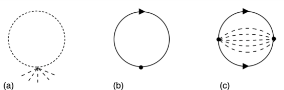
Figure 1: List of divergent diagrams: (a) scalar tadpole; (b) fermionic tadpole ; (c) two-vertex fermionic loop, dressed by an arbitrary number of internal scalar propagators.

The degree of divergence of a loop diagram $D_{\Lambda}$ is easily computed: zappalast

$$D_{\Lambda}=6\,\left(1-\sum_{n}V_{n}\right)\,,$$ (3)

where $V_{n}$ is the number of vertices with $n$ legs (proportional to $g_{n}$). We notice that $D_{\Lambda}$ does not depend on the number of external legs and it is always negative unless the diagram has one vertex only, $V_{\widehat{n}}=1$ and $V_{n}=0$ for $n\neq\widehat{n}$, regardless the specific value of $\widehat{n}$. Then, one concludes that the only primitively divergent scalar diagrams are those with one vertex, an arbitrary number of external legs, and an arbitrary number of tadpoles, all insisting on the same vertex. As an example, the diagram with one tadpole and five external legs is displayed in Fig. 1 and labelled with (a).

The first consequence of this analysis is that loop diagrams with two or more vertices are not divergent and, since only diagrams with more than one vertex can carry dependence on some external momentum, it follows that quantum corrections depending on external momenta must be finite. In particular, corrections to the parameters $a_{k}$ in Eq. (1) come from external momentum dependent two-point diagrams and, therefore, they are finite. An explicit calculation in zappalast , shows that these corrections, at least at energy scales above $M$, are certainly negligible.

The second consequence comes from the observation that also all operators proportional to $w_{m,k}$ get quantum corrections from diagrams that depend on some external momentum and therefore, when the constraint $w_{m,k}=0$ is enforced in (2), no significant divergent correction to this constraint is generated. Then, the dangerous corrections to the speed of light are avoided in a consistent way.

The tadpole (a) in Fig. 1, gives the elementary UV divergence. It is a one loop diagram that, following zappalast , can be regularized by adopting the non-Lorentz invariant cutoff on the modulus of the tri-momentum, which is consistent with the non-Lorentz invariant structure of the action in Eq. (1). Since we are interested in the UV properties of the theory, we integrate the tadpole between two momentum scales $\Lambda_{1}$ and $\Lambda_{2}$, with $\Lambda_{1}>>\Lambda_{2}>>M$ and we assume $M$ to be much larger than any scale appearing in Eqs. (1) and (2) that, consequently, will be neglected.

Then, for the tadpole (a), we get:

$$I_{1}(\Lambda_{1},\Lambda_{2},M)=\frac{M^{2}}{\sqrt{a_{3}}\,(2\pi)^{2}}\ln\left(\frac{\Lambda_{1}}{\Lambda_{2}}\right)+O\left(\frac{M^{4}}{\Lambda_{2}^{2}},\,\frac{M^{2}\Lambda_{2}^{2}}{\Lambda_{1}^{2}}\right)\,.$$ (4)

where, without any loss of generality, we can put $a_{3}=1$. zappalast

If we now compute the quantum corrections of a generic coupling $g_{n}$, the combinatorial factors of each contributing diagram always yield the following series (which corresponds to the exponential series, if the various couplings are neglected):

$$g_{n}(\Lambda_{2})=\sum_{m=0}^{\infty}\frac{g_{{}_{n+2m}}(\Lambda_{1})}{m!}\;\left[\frac{I_{1}(\Lambda_{1},\Lambda_{2},M)}{2M^{2}}\right]^{m}$$ (5)

The series in (5) is simplified if one assumes that the theory has only one coupling, i.e. $g_{n}=g$ for all $n$. In fact, in this case by using Eq. (4), one finds

$$g(\Lambda_{2})=g(\Lambda_{1})\;\exp\left[\frac{I_{1}(\Lambda_{1},\Lambda_{2},M)}{2M^{2}}\right]\simeq g(\Lambda_{1})\;\left(\frac{\Lambda_{1}}{\Lambda_{2}}\right)^{1/\left(8\pi^{2}\right)}$$ (6)

and it is straightforward to check that $g(\Lambda_{1})\to 0$ in the limit $\Lambda_{1}\to\infty$, at fixed $g(\Lambda_{2})$, i.e. the coupling $g$ is asymptotically free.

This remarkable result can be easily generalized to the case of different $g_{n}$ if, at the scale $\Lambda_{1}$, the set of all $g_{n}$ is bounded by $0\leq g_{n}\leq g$, where $g$ is a real number. Then, the exponential series in (6) is greater than the series (5) term by term, and it is straightforward to conclude $g_{n}(\Lambda_{1})\to 0$ for each $n$, when $\Lambda_{1}\to\infty$. Conversely, if the potential term in Eq. (1) contains only a finite set of non-zero couplings $g_{n}\neq 0$, the theory is renormalizable, but no asymptotically free coupling is found. zappalast

III Fermionic Fields

In case of fermionic degrees of freedom, the higher derivative part of the 3+1 dimensional action, with $z=3$, is

$$S_{F}=\!\int\!d^{3}x\,dt\;\bar{\psi}\left[i\gamma^{0}\partial_{0}-\left(b_{1}+\,\frac{\partial_{j}\partial^{j}}{M^{2}}\right)(i\gamma^{i}\partial_{i})-m_{f}\right]\,\psi$$ (7)

where the summed indices $j$ and $i$ refer to the 3 space coordinates and, as for the scalar case, we normalize $S_{F}$ by setting $b_{3}=1$ in front of the higher derivative term. To preserve rotational invariance, the higher derivative part in brackets does not contain a $b_{2}$ term (analogous of the $a_{2}$ term in (1) ), although the essential terms, linear and cubic in the space derivatives, are included in (7). The linear term in the time derivative sets the scaling dimension of the fermion field, $[\psi]_{s}=3/2$, which, unlike the scalar field, turns out to be equal to its canonical dimension.

Consequently, if we assume a Yukawa-like interaction with the scalar excitations, the renormalizable interaction sector of the action is

$$S_{Y}=-\!\int\!d^{3}x\,dt\;\sum_{n=1}^{\infty}\,y_{n}\;\frac{\bar{\psi}\psi\;\phi^{n}}{n!\;M^{n-1}}\,,$$ (8)

where all powers of the scalar field are taken into account because $[\phi]_{s}=0$ and, therefore, all these terms are renormalizable.

The analysis of the degree of divergence of the diagrams generated by $S_{Y}$ yields

$$D_{\Lambda}=6-3\,\sum_{n}Y_{n}-\frac{3}{2}E_{f}$$ (9)

where $Y_{n}$ is the number of vertices proportional to $y_{n}$ and $E_{f}$ is the number of external fermionic legs. Then $D_{\Lambda}$ is non-negative if $E_{f}=2$ and $\sum_{n}Y_{n}=1$, or $E_{f}=0$ and $\sum_{n}Y_{n}=1$, or $E_{f}=0$ and $\sum_{n}Y_{n}=2$. In the first case, when $E_{f}=2$, diagrams have, besides the two external fermionic legs, all possible multiple scalar tadpoles insisting on the same vertex. In the second case, with $E_{f}=0$, diagrams display the fermionic tadpole (b) in Fig. 1, together with all possible multiple scalar tadpoles insisting on the same vertex. In the third case, again with $E_{f}=0$, diagrams are of the (c) kind in Fig. 1, where not only each vertex can be dressed with all possible multiple scalar tadpoles as before, but also an arbitrary number of internal scalar propagators can link the two vertices. In all three cases, an arbitrary number of scalar external legs coming out of each vertex is allowed. Then, in the diagrams (b) and (c) the vertices indicated by thick black dots, stand for the full sum of scalar tadpoles together with the arbitrary number of scalar external legs.

By adopting the same regularization procedure employed for scalar fields, the fermionic tadpole (b) gives the negative result $-4m_{f}I_{1}$, and the most divergent part of the diagram (c), with $r\neq 0$ internal scalar propagators, is $-2I_{1}^{r+1}$ while the pure fermionic one loop diagram (c) without scalar propagators gives $-4I_{1}$. Therefore, in all cases the divergences amount to powers of the logarithm of the cutoff.

It is now possible to analyze the renormalization of the couplings and we consider the Yukawa sector in the simple case in which all couplings are equal: $y=y_{n}$. For our purposes, together with $a_{3}=b_{3}=1$, which is justified by the negligible running of these couplings in the region above $M$, we can also take $a_{1}=a_{2}=b_{1}=0$ without loss of generality. The sum of all diagrams contributing to the renormalization of $y$, integrated as before between the two scales $\Lambda_{1}$ and $\Lambda_{2}$, gives

$$y(\Lambda_{2})=y(\Lambda_{1})\;\exp\left[\frac{I_{1}(\Lambda_{1},\Lambda_{2},M)}{2M^{2}}\right]\equiv y(\Lambda_{1})\;{\cal E}$$ (10)

and this leads to the same conclusions discussed after Eq. (6), i.e. the coupling $y$ is asymptotically free.

The renormalization of the scalar sector is more involved, because of the diagrams in (c). In fact, by keeping different $g_{n}$ for different $n$, and by retaining the leading divergences only, we find the following generalization of Eq. (5)

$$g_{n}(\Lambda_{2})=\sum_{m=0}^{\infty}\frac{g_{{}_{n+2m}}(\Lambda_{1})}{m!}\;\left[\frac{I_{1}(\Lambda_{1},\Lambda_{2},M)}{2M^{2}}\right]^{m}-c_{n}\;y(\Lambda_{1})^{2}\;{\cal E}^{4}I_{1}$$ (11)

where $c_{n}>0$ is associated with the combinatorial weight of the diagrams in (c) and its value changes with $n$. Then, also the contribution to $g_{n}$ changes with $n$. Therefore, if all $g_{n}$ were equal to a single coupling $g$ as for the case of the Yukawa coupling $y$, it would be impossible to renormalize the full structure in Eq. (11).

In order to determine the $\beta$-function of $g_{n}$, it is sufficient to take the derivative with respect to $\Lambda_{2}$ in Eq. (11), by keeping fixed the values of all couplings at $\Lambda_{1}$, and it is easy to realize that the two terms in the right hand side (rhs) of (11) give respectively a negative and positive contribution, so that the sign of the $\beta$-function depends on the balance of these contributions and, consequently, on the particular values of the couplings, so that it is not uniquely established.

However, the following heuristic argument can be put forward: the stability of the scalar potential requires $g_{n}\geq 0$, at least for all $n$ larger than some $\bar{n}$. Then, for $n\geq\bar{n}$ the first term in the rhs of (11) must be larger than the second. In addition, we noticed that the coupling $y$ is asymptotically free and it grows when the momentum scale is lowered and, in case the $g_{n}$ are not sufficiently large at the scale $\Lambda_{1}$ to ensure a negative $\beta$-function, $g_{n}$ decreases when the momentum scale runs from $\Lambda_{1}$ towards $\Lambda_{2}$. Then, if these two scales are sufficiently distant, $g_{n}$ could become negative at the infrared scale $\Lambda_{2}$, yielding an unstable potential. This is avoided if the values of $g_{n}(\Lambda_{1})$ are sufficiently large to ensure a negative $\beta$-function, at least for all $g_{n}$ with $n\geq\bar{n}$.

It must be noticed that, in the analysis of the fermionic sector we deliberately did not include 2n-fermion vertices. Actually, it is easy to show by means of the analysis of the degree of divergence of diagrams, that the only vertex of this kind that is renormalizable, is the 4-fermion vertex. However, this vertex can always be reduced, through Hubbard-Stratonovich transformation to a Yukawa-like interaction and, therefore, it should not be treated as a fundamental interaction. In any case, the 4-fermion interaction was already studied, Dhar:2009dx and we do not expect that its inclusion could substantially modify our conclusions.

A comment on the scalar square mass $g_{2}\;M^{2}$ ( as defined in (2) ), whose correction is given in (11) for $n=2$, is in order. It is evident that, unless a very subtle cancellation between the first and second term in the rhs of (11) occurs, we get a finite non-vanishing correction to the scalar mass from the momentum region between $\Lambda_{1}$ and $\Lambda_{2}$, with $\Lambda_{1}\to\infty$. The correction is, in any case, proportional to the scale $M^{2}$. This is analogous to the result obtained for the scalar case in zappalast , and even if, as expected, the fermionic contribution to the correction occurs here with opposite sign with respect to the scalar, an exact cancellation of the two would be quite unnatural.

IV Gauge Fields

The inclusion of gauge fields can be realized by defining the appropriate covariant derivative, which can be constructed by starting from the generalized derivative $\widehat{\partial}_{\mu}$ already introduced in Eq. (7) (here for simplicity, the coefficients of the various derivative terms, analogous of $b_{1},\,b_{3}$, are taken equal to 1)

$$\widehat{\partial}_{0}=\partial_{0}\;,\;\;\;\;\;\;\;\;\widehat{\partial}_{i}=\left(1+\,\frac{\partial_{j}\partial^{j}}{M^{2}}\right)\partial_{i}\;,$$ (12)

and by including the gauge field in the usual way : $\widehat{D}_{\mu}=\widehat{\partial}_{\mu}-iqA_{\mu}$. Accordingly, the generalized electromagnetic tensor is $\widehat{F}_{\mu\nu}=\widehat{\partial}_{\mu}A_{\nu}-\widehat{\partial}_{\nu}A_{\mu}$. However, it is straightforward to realize that $\widehat{D}_{\mu}$, which is non-linear in the derivatives, does not behave properly under gauge transformations, so that the corresponding higher derivative electrodynamics produces gauge violating contributions to the amplitudes, proportional to powers of $p^{2}/M^{2}$, where $p^{2}=p^{\mu}p_{\mu}$ is some square momentum scale, representative of the amplitude.

A different higher derivative formulation, that is gauge invariant, was already proposed long agohorava:ym but, in this case, the higher order space derivatives appear in the form $(D_{h}D_{j}F_{ik})^{2}$ (where $D_{i}$ are the space components of the standard covariant derivative), which contains terms analogous to those proportional to $w_{m,k}$ in Eq. (2) for the scalar case. As discussed above, in order to avoid model dependent modifications of the light cone, we required to reject these kind of terms and, consequently, this formulation cannot be accepted.

If we admit that, together with Lorentz symmetry, also gauge invariance is violated, at least at high energy, and only recovered at low energies below $M$, we can make use of the definition in (12) and of the corresponding $\widehat{D}_{\mu}$, to include the dynamics of the field $A_{\mu}$. Then, independently of gauge symmetry, the effect of the dynamics of $A_{\mu}$ in Eq. (11) is, from an effective point of view, equivalent to the presence of additional scalar degrees of freedom, with the consequence of modifying only some coefficients in (11) but not the overall structure of the equation, so that the conclusions discussed above are not qualitatively altered.

V Conclusions

We analyzed a realization of a higher derivative theory in 3+1 dimensions with anisotropy exponent $z=3$ and, in particular, we considered the possible generalization to fermionic and vector gauge fields of the specific formulation for scalar fields studied in zappalast , with the main intent of constructing a consistent UV completion of these fields and, ultimately, of the Standard Model. Therefore, we focused on the high energy region that corresponds to energies much larger than the scale $M$, which sets the scale of Lorentz violating effects.

In fact, as evident from Eqs. (1) and (7), all modifications to the standard Lorentz invariant dispersion relations of scalars and fermions, correspond to Lorentz violating additive corrections proportional to powers of the ratio $(p^{2}/M^{2})$, which become relevant only for $p^{2}>>M^{2}$. In addition, an acceptable crossover to the region below $M^{2}$, where the usual renormalization group flow of the various couplings is recovered and Lorentz, as well as gauge symmetry are effectively restored, has been realized and discussed in zappalast . As already mentioned, astrophysical high energy gamma ray observations put a strong limit on $M$, that, for models with corrections proportional to $(p^{2}/M^{2})$ as in our case, is about $M\geq 10^{10}$ GeV,ellis:2003 ; chenhuang a very large value if compared with the characteristic scales of the Standard Model.

From the point of view of renormalizability, there is a great improvement due to the higher derivative terms. In particular, the scalar self-interacting sector has a very simple UV structure that indicates that the couplings $g_{n}$ are asymptotically free, at least when, at the scale $M$, all couplings are positive and the set of all $g_{n}$ is bounded from above; in addition, if $g_{n}=g$ for all $n$, the series of significant diagrams, due to their combinatorial weights, sums up to a simple exponential form.

The interacting system of scalars and fermions reproduces the same structure of divergences in the Yukawa sector with asymptotic freedom of the corresponding coupling, while for the scalar couplings the pattern of divergences becomes more complicated. However, under the hypothesis of stability of the potential, also scalar couplings turn out to be asymptotically free. On the other hand, we are not able to include gauge fields without introducing interaction operators that produce physically unacceptable modifications of the light cones for different species of particles. Therefore in this approach, gauge symmetry can only be recovered as an emergent low energy symmetry (below $M$).

Then, from the phenomenological point of view, if the violation of both Lorentz and gauge symmetry could be kept under control by the large value of the lower bound on $M$, the price to pay is that the strong suppression of divergences is limited to the UV region above $M$, while standard scaling holds at scales smaller than $M$. In particular, the correction to the scalar square mass, although finite, is proportional to $g_{4}M^{2}$, that is very large if compared for instance to the Higgs square mass. In this sense, the positive features of this kind of theory, seem to have a very weak impact on the physics of the Standard Model at present energies.

References

- (1) W. Thirring, Phys. Rev. 77, 570 (1950).
- (2) A. Pais and G. E. Uhlenbeck, Phys. Rev. 79, 145 (1950).
- (3) K. S. Stelle, Phys. Rev. D 16, 953 (1977).
- (4) F. J. de Urries and J. Julve, J. Phys. A 31, 6949 (1998). [hep-th/9802115].
- (5) S. W. Hawking and T. Hertog, Phys. Rev. D 65, 103515 (2002). [hep-th/0107088].
- (6) J. Collins, A. Perez, D. Sudarsky, L. Urrutia, and H. Vucetich, Phys. Rev. Lett. 93, 191301 (2004). [arXiv:gr-qc/0403053].
- (7) R. Hornreich, M. Luban, and S. Shtrikman, Phys.Rev.Lett. 35, 1678 (1975).
- (8) R. M. Hornreich, Journal of Magnetism and Magnetic Materials 15, 387 (1980).
- (9) W. Selke, Physics Reports 170, 213 (1988).
- (10) H. Diehl, Acta Phys.Slov. 52, 271 (2002).
- (11) H. Diehl and M. Shpot, J.Phys. A35, 6249 (2002). [cond-mat/0204267].
- (12) J. Ellis, N. Mavromatos, D.V. Nanopoulos, A.S. Sakharov Astron. Astrophys. 402, 409 (2003). [arXiv:astro-ph/0210124].
- (13) B. Chen, Q.G. Huang, Phys. Lett. B 683, 108 (2010).
- (14) J. Ellis, R. Konoplich, N. E. Mavromatos, L. Nguyen, A. S. Sakharov, and E. K. Sarkisyan-Grinbaum, Phys. Rev. D 99, 083009 (2019). [arXiv:1807.00189].
- (15) A. Bonanno and D. Zappala, Nucl. Phys. B 893, 501 (2015). [arXiv:1412.7046].
- (16) D. Zappala, Phys. Lett. B 773, 213 (2017). [arXiv:1703.00791].
- (17) D. Zappala, Phys. Rev. D 98, 085005 (2018). [arXiv:1806.00043].
- (18) D. Zappala, Int. J. Geom. Meth. Mod. Phys. 17, 2050053 (2020). [arXiv:1912.03071].
- (19) N. Defenu, A. Trombettoni, and D. Zappala, Nucl. Phys. B 964, 115295 (2021). [arXiv:2003.04909].
- (20) D. Buccio and R. Percacci, Renormalization Group flows between Gaussian Fixed Points, [arXiv:2207.10596].
- (21) R. P. Woodard, Lect. Notes Phys. 720, 403 (2007). [astro-ph/0601672].
- (22) P. Horava, Phys. Rev. D 79, 084008 (2009). [arXiv:0901.3775].
- (23) A.O. Barvinsky, D. Blas, M. Herrero-Valea, S.M. Sibiryakov, and C.F. Steinwachs, Phys. Rev. D 93, 064022 (2016). [arXiv:1512.02250].
- (24) A.O. Barvinsky, D. Blas, M. Herrero-Valea, S.M. Sibiryakov, and C.F. Steinwachs, Phys. Rev. Lett. 119, 211301 (2017). [arXiv:1706.06809].
- (25) A.O. Barvinsky, D. Blas, M. Herrero-Valea, and S.M. Sibiryakov, Phys. Rev. D 100, 026012 (2019). [arXiv:1905.03798].
- (26) A.O. Barvinsky, A.V. Kurov, and S.M. Sibiryakov, Phys. Rev. D 105, 044009 (2022). [arXiv:2110.14688].
- (27) D. Anselmi and M. Halat, Phys. Rev. D 76,125011 (2007). [arXiv:0707.2480].
- (28) R. Iengo, J. G. Russo, and M. Serone, JHEP 11, 020 (2009). [arXiv:0906.3477].
- (29) A. Dhar, G. Mandal, and S. R. Wadia, Phys. Rev. D 80, 105018 (2009). [arXiv:0905.2928].
- (30) P. Horava, Phys. Lett. B 694, 172 (2011). [arXiv:0811.2217].
- (31) M. Eune, W. Kim, and E. J. Son, Phys. Lett. B 703, 100 (2011). [arXiv:1105.5194].
- (32) J. Alexandre, Int. J. Mod. Phys. A 26, 4523 (2011). [arXiv:1109.5629].
- (33) K. Kikuchi, Prog. Theor. Phys. 127, 409 (2012). [arXiv:1111.6075].
- (34) W. Chao, Commun. Theor. Phys. 65, 743 (2016). [arXiv:0911.4709].
- (35) A. R. Solomon and M. Trodden, JCAP 02, 031 (2018). [arXiv:1709.09695].
- (36) D. Zappala, Eur. Phys. J. C 82, 341 (2022). [arXiv:2111.08385].