Stochastic Optimization of 3D Non-Cartesian Sampling Trajectory (SNOPY)

Abstract

1 Purpose

Optimizing 3D k-space sampling trajectories for efficient MRI is important yet challenging. This work proposes a generalized framework for optimizing 3D non-Cartesian sampling patterns via data-driven optimization.

2 Methods

We built a differentiable MRI system model to enable gradient-based methods for sampling trajectory optimization. By combining training losses, the algorithm can simultaneously optimize multiple properties of sampling patterns, including image quality, hardware constraints (maximum slew rate and gradient strength), reduced peripheral nerve stimulation (PNS), and parameter-weighted contrast. The proposed method can either optimize the gradient waveform (spline-based freeform optimization) or optimize properties of given sampling trajectories (such as the rotation angle of radial trajectories). Notably, the method optimizes sampling trajectories synergistically with either model-based or learning-based reconstruction methods. We proposed several strategies to alleviate the severe non-convexity and huge computation demand posed by the high-dimensional optimization. The corresponding code is organized as an open-source, easy-to-use toolbox.

3 Results

We applied the optimized trajectory to multiple applications including structural and functional imaging. In the simulation studies, the reconstruction PSNR of a 3D kooshball trajectory was increased by 4 dB with SNOPY optimization. In the prospective studies, by optimizing the rotation angles of a stack-of-stars (SOS) trajectory, SNOPY improved the PSNR by 1.4 dB compared to the best empirical method. Optimizing the gradient waveform of a rotational EPI trajectory improved subjects’ rating of the PNS effect from ‘strong’ to ‘mild.’

4 Conclusion

SNOPY provides an efficient data-driven and optimization-based method to tailor non-Cartesian sampling trajectories.

5 Introduction

Most magnetic resonance imaging systems sample data in the frequency domain (k-space) following prescribed sampling trajectories. Efficient sampling strategies can accelerate acquisition and improve image quality. Many well-designed sampling strategies and their variants, such as spiral, radial, CAIPIRINHA, and PROPELLER ^{1, 2, 3, 4}, have enabled MRI’s application to many areas ^{5, 6, 7, 8}. Sampling patterns in k-space either are located on the Cartesian raster or arbitrary locations (non-Cartesian sampling). This paper focuses on optimizing 3D non-Cartesian trajectories and introduces a generalized gradient-based optimization method for automatic trajectory design/tailoring.

The design of sampling patterns usually considers certain properties of k-space signals. For instance, the variable density (VD) spiral trajectory ⁹ samples more densely in the central k-space where more energy is located. For higher spatial frequency regions, the VD spiral trajectory uses larger gradient strengths and slew rates to cover as much of k-space as quickly as possible. Compared to 2D sampling, designing 3D sampling by hand is more challenging for several reasons. The number of parameters increases in 3D, and thus the parameter selection is more difficult due to the larger search space. Additionally, analytical designs usually are based on the Shannon-Nyquist relationship ^{10, 11, 12} that might not fully consider properties of sensitivity maps and advanced reconstruction methods. For 3D sampling pattern with a high undersampling (acceleration) ratio, there are limited analytical tools for designing sampling patterns having anisotropic FOV and resolution. The peripheral nerve stimulation (PNS) effect is also more severe in the 3D imaging ¹³, further complicating analytical trajectory designs. For these reasons, it is important to automate the design of 3D sampling trajectories.

Many 3D sampling approaches exist. ‘stack-of-2D’ is a commonly used 3D sampling strategy, by stacking 2D sampling patterns in the slice direction ^{6, 13}. This approach is easier to implement and enables slice-by-slice 2D reconstruction. Another design applies Cartesian sampling in the frequency-encoding direction and non-Cartesian sampling in the phase-encoding direction ^{14, 15}. However, these approaches do not fully exploit the potential of modern gradient systems and may not perform as well as true 3D sampling trajectories ¹⁶.

Recently, 3D SPARKLING ¹⁶ proposes to optimize 3D sampling trajectories based on the goal of conforming to a given density while distributing samples as uniformly as possible ¹⁷. That method demonstrated improved image quality compared to the ‘stack-of-2D SPARKLING’ approach. In both 2D and 3D, the SPARKLING approach uses a pre-specified sampling density in k-space that is typically an isotropic radial function. This density function cannot readily capture distinct energy distributions of different imaging protocols. Additionally, the method does not control PNS effects explicitly. SPARKLING optimizes the location of every sampling point, or the gradient waveform (freeform optimization), and is not applicable to the optimization of existing parameters of existing sampling patterns, which limits its practicability beyond T2^∗-weighted imaging.

In addition to analytical methods, learning-based methods are also investigated in MRI sampling trajectory design. Since different anatomies have distinct energy distributions in the frequency domain, an algorithm may learn to optimize sampling trajectories from training datasets. Several studies show that different anatomies and different reconstruction algorithms produce very different optimized sampling patterns, and such optimized sampling trajectories can improve image quality ^{18, 19, 20, 21, 22, 23, 24, 25, 26}. Several recent studies also applied learning-based approaches to 3D non-Cartesian trajectory design. J-MoDL ¹⁴ proposes to learn sampling patterns and model-based deep learning reconstruction algorithms jointly. J-MoDL optimizes the sampling locations in the phase-encoding direction, to avoid the computation cost of non-uniform Fourier transform. PILOT/3D-FLAT ²⁷ jointly optimizes freeform 3D non-Cartesian trajectories and a reconstruction neural network with gradient-based methods. These studies use the standard auto-differentiation approach to calculate the gradient, which can be inaccurate and lead to sub-optimal optimization results ^{19, 28}.

This work extends our previous methods ^{19, 28} and introduces a generalized Stochastic optimization framework for 3D NOn-Cartesian samPling trajectorY (SNOPY). The proposed method can automatically tailor given trajectories and learn k-space features from training datasets. We formulated several optimization objectives, including image quality, hardware constraints, PNS effect suppression, and image contrast. Users can simultaneously optimize one or multiple characteristics of a given sampling trajectory. Similar to previous learning-based methods ^{14, 19, 20, 21}, the sampling trajectory can be jointly optimized with trainable reconstruction algorithms to improve image quality. The joint optimization approach can exploit the synergy between acquisition and reconstruction, and learn optimized trajectories for different anatomies. The algorithm can optimize various properties of a sampling trajectory, such as the readout waveform, or the rotation angles of readout shots, making it more practical and applicable. We also introduced several techniques to improve efficiency, enabling large-scale 3D trajectory optimization. We tested the proposed methods with multiple imaging applications, including structural and functional imaging. These applications benefited from the SNOPY-optimized sampling trajectories in both simulation and prospective studies.

6 Theory

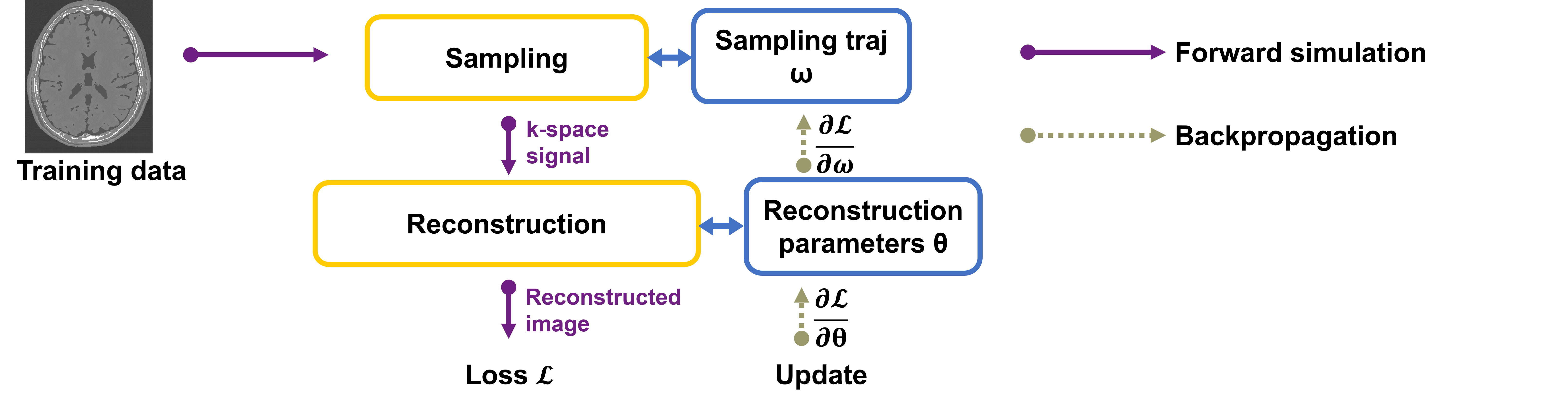
Figure 1:  Diagram of SNOPY. The sampling trajectory (and possibly reconstruction parameters) are updated using gradient methods. The training/optimization uses the differentiable programming approach to get the gradient required in the update.

This section describes the proposed gradient-based methods for trajectory optimization. We use the concept of differentiable programming to compute the Jacobian/gradient w.r.t. sampling trajectories required in the gradient-based methods. The sampling trajectory and reconstruction parameters are differentiable parameters, whose gradients can be calculated by auto-differentiation or chain rule. To learn/optimize these parameters, one may apply (stochastic) gradient descent-like algorithms. Fig. 1 illustrates the basic idea. Here the sampling trajectory can also be jointly optimized with the parameters of a learnable reconstruction algorithm, so that the learned sampling trajectory and reconstruction method are in synergy and can produce high-quality images. The SNOPY algorithm combines several optimization objectives, to ensure that the optimized sampling trajectories have desired properties. 6.1 delineates these objective functions. 6.3 shows that the proposed method is applicable to multiple scenarios with different parameterization strategies. For non-Cartesian sampling, the system model usually involves non-uniform fast Fourier transforms (NUFFT). 6.4 briefly describes an efficient and accurate way to calculate the gradient involving NUFFTs. 6.5 suggests several engineering approaches to make this large-scale optimization problem practical and efficient.

6.1 Optimization objectives

This section describes the optimization objectives. Since we propose to use a stochastic gradient descent-type optimization algorithm, the objective function, or loss function, is by default defined on a mini-batch of data. The final loss function can be a linear combination of the following loss terms to ensure the optimized trajectory has multiple desired properties.

6.1.1 Image quality

For many MRI applications, efficient acquisition and reconstruction aim to produce high-quality images. Consequently, the learning objective should encourage images reconstructed from sampled k-space signals to be close to the reference image. We formulate this similarity objective as the following image quality training loss:

$$\mathcal{L}_{\mathrm{recon}}=\|f_{\bm{\theta},\bm{\omega}}(\bm{A}(\bm{\omega})\bm{x}+\bm{\varepsilon})-\bm{x}\|.$$ (1)

Here, $\bm{\omega}(\bm{c})\in\mathbb{R}^{N_{\mathrm{fe}}\times N_{\mathrm{s}}\times N_{\mathrm{d}}}$ denotes the trajectory to be optimized, with $N_{\mathrm{s}}$ shots, $N_{\mathrm{fe}}$ sampling points in each shot, and $N_{\mathrm{d}}$ image dimensions. $\bm{c}$ denotes the parameterization coefficients introduced in 6.3. For 3D MRI, $N_{\mathrm{d}}=3$. $\bm{x}$ is a mini-batch of data from the training set $\mathcal{X}$. $\bm{\varepsilon}$ is simulated complex Gaussian noise. $\bm{A}(\bm{\omega})$ is the forward system matrix for sampling trajectory $\bm{\omega}$ ²⁹. $\bm{A}$ can also incorporate multi-coil sensitivity information ³⁰ and field inhomogeneity ³¹. $\bm{\theta}$ denotes the reconstruction algorithm’s parameters. It can be kernel weights in a convolutional neural network (CNN), or the regularizer coefficient in a model-based reconstruction method. The term $\|\cdot\|$ can be $\ell_{1}$ norm, $\ell_{2}$ norm, or a combination of both. There are also other ways to measure the distance between $\bm{x}$ and $f_{\bm{\theta},\bm{\omega}}(\bm{A}(\bm{\omega})\bm{x}+\bm{\varepsilon})$, such as the structural similarity index (SSIM ³²). For simplicity, this work used a linear combination of $\ell_{1}$ norm and square-of-$\ell_{2}$ norm.

6.1.2 Hardware limits

The gradient system of MR scanners has physical constraints, namely maximum gradient strength and slew rate. Ideally, we would like to enforce a set of constraints of the form

$$\|\bm{g}_{i}[j,:]\|_{2}\leq g_{\mathrm{max}},\quad\bm{g}_{i}=\bm{D}_{1}\bm{\omega}[:,i,:]/(\gamma\Delta t)\in\mathbb{R}^{(N_{\mathrm{fe}}-1)\times N_{\mathrm{d}}},$$

for every shot $i=1,\ldots,N_{\mathrm{s}}$ and time sample $j=1,\ldots,N_{\mathrm{fe}}$, where $\bm{g}_{i}$ denotes the gradient strength of the $i$ shot and $g_{\max}$ denotes the desired gradient upper bound. We use a Euclidean norm along the spatial axis so that any 3D rotation of the sampling trajectory still obeys the constraint. A similar constraint is enforced on the Euclidean norm of the slew rate $\bm{s}_{i}=\bm{D}_{2}\bm{\omega}[:,i,:]/(\gamma\Delta t^{2}),$ where $\bm{D}_{1}$ and $\bm{D}_{2}$ denote first-order and second-order finite difference operators applied along the readout dimension, and $\Delta t$ is the raster time interval and $\gamma$ is the gyromagnetic ratio.

To make the optimization more practical, we follow previous studies ^{19, 21}, and formulate the hardware constraint as a soft penalty term:

$$\mathcal{L}_{\mathrm{g}}=\sum_{i=1}^{N_{\mathrm{s}}}\sum_{j=1}^{N_{\mathrm{fe}}-1}\phi_{g_{\max}}(\|\bm{g}_{i}[j,:]\|_{2})$$ (2)

$$\mathcal{L}_{\mathrm{s}}=\sum_{i=1}^{N_{\mathrm{s}}}\sum_{j=1}^{N_{\mathrm{fe}}-2}\phi_{s_{\max}}(\|\bm{s}_{i}[j,:]\|_{2}).$$ (3)

Here $\phi$ is a penalty function, and we use a soft-thresholding function $\phi_{\lambda}(x)=\max(|x|-\lambda,0).$ Since $\phi$ here is a soft penalty and the optimization results may exceed $s_{\max}$ and $g_{\max}$, $s_{\max}$ and $g_{\max}$ can be slightly lower than the scanner’s physical limits to make the optimization results feasible on the scanner.

6.1.3 Suppression of PNS effect

3D imaging often leads to stronger PNS effects than 2D imaging because of the additional gradient axis. To quantify possible PNS effects of candidate gradient waveforms, we used the convolution model in Ref. schulte:2015:PNS:

$$R_{id}(t)=\frac{1}{s_{\min}}\int_{0}^{t}\frac{\bm{s}_{id}(\theta)c}{(c+t-\theta)^{2}}d\theta,$$ (4)

where $R_{id}$ denotes the PNS effect of the gradient waveform from the $i$th shot and the $d$th dimension. $\bm{s}_{id}$ is the slew rate of the $i$th shot in the $d$th dimension. $c$ (chronaxie) and $s_{\min}$ (minimum stimulation slew rate) are scanner parameters.

Likewise, we discretize the convolution model and formulate a soft penalty term as the following loss function:

$$\bm{p}_{id}[j]=\sum_{k=1}^{j}\frac{\bm{s}_{id}[j]c\Delta t}{s_{\min}(c+j\Delta t-k\Delta t)^{2}},$$

$$\mathcal{L}_{\mathrm{pns}}=\sum_{i=1}^{N_{\mathrm{s}}}\sum_{j=1}^{N_{\mathrm{fe}}}\phi_{p_{\max}}((\sum_{d=1}^{N_{\mathrm{d}}}\bm{p}_{id}[j]^{2})^{\frac{1}{2}}).$$ (5)

Again, $\phi$ denotes the soft-thresholding function, with PNS threshold $p_{\max}$ (usually $\leq 80\%$³³). This model combines the 3 spatial axes via the sum-of-squares manner, and does not consider the anisotropic response of PNS ³⁴. The implementation may use an FFT (with zero padding) to implement this convolution efficiently.

6.1.4 Image contrast

In many applications, the optimized sampling trajectory should maintain certain parameter-weighted contrasts. For example, ideally the (gradient) echo time (TE) should be identical for each shot. Again we replace this hard constraint with an echo time penalty. Other parameters, like repetition time (TR) and inversion time (TI), can be predetermined in the RF pulse design. Specifically, the corresponding loss function encourages the sampling trajectory to cross the k-space center at certain time points:

$$\mathcal{L}_{c}=\sum_{\{i,j,d\}\in C}\phi_{0}(|\bm{\omega}[i,j,d]|),$$ (6)

where $C$ is a collection of gradient time points that are constrained to cross k-space zero point. $\phi$ is still a soft-thresholding function, with threshold 0.

6.2 Reconstruction

In (1), the reconstruction algorithm $f_{\bm{\theta},\bm{\omega}}(\cdot)$ can be various algorithms. Consider a typical cost function for regularized MR image reconstruction

$$\hat{\bm{x}}=\operatornamewithlimits{arg\,min}_{\bm{x}}\|\bm{A}(\bm{\omega})\bm{x}-\bm{y}\|_{2}^{2}+\mathcal{R}(\bm{x}).$$ (7)

$\mathcal{R}(\bm{x})$ here can be a Tikhonov regularization $\lambda\|\bm{x}\|_{2}^{2}$ (CG-SENSE ³⁵), a sparsity penalty $\lambda\|\bm{T}\bm{x}\|_{1}$ (compressed sensing ³⁶, $\bm{T}$ is a finite-difference operator), a roughness penalty $\lambda\|\bm{T}\bm{x}\|_{2}^{2}$ (penalized least squares, PLS), or a neural network (model-based deep learning, MoDL ³⁷). The Results section shows that different reconstruction algorithms lead to distinct optimized sampling trajectories.

To get a reconstruction estimation $\hat{\bm{x}}$, one may use corresponding iterative reconstruction algorithms. Specifically, the algorithm should be step-wise differentiable (or sub-differentiable) to enable differentiable programming. The backpropagation uses the chain rule to traverse every step of the iterative algorithm to calculate the gradient w.r.t. variables such as $\bm{\omega}$.

6.3 Parameterization

As is shown in Ref. wang:22:bjork-tmi, directly optimizing every k-space sampling point (or equivalently every gradient waveform time point) may lead to sub-optimal results. Additionally, in many applications one wants to optimize certain properties of existing sampling patterns, such as the rotation angles of a multi-shot spiral trajectory, so that the optimized trajectory can be easily integrated into existing workflows. For these cases, we propose two parameterization strategies.

The first approach, spline-based freeform optimization, is to represent the sampling pattern using a linear basis, i.e., $\bm{\omega}=\bm{B}\bm{c}$, where $\bm{B}$ is a matrix of samples of a basis such as quadratic B-spline kernels and $\bm{c}$ denotes the coefficients to be optimized ^{19, 21}. This approach fully exploits the generality of a gradient system. Using a linear parameterization like B-splines reduces the degrees of freedom and facilitates applying hardware constraints ^{19, 38}. Additionally, it enables multi-scale optimization for avoiding sub-optimal local minima and further improving optimization results ^{17, 19, 21}. However, the freeformly optimized trajectory could have implementation challenges. For example, some MRI systems can not restore hundreds of different gradient waveforms.

The second approach is to optimize attributes ($\bm{c}$) of existing trajectories such as rotation angles, where $\bm{\omega}(\bm{c})$ is a nonlinear function of the parameters. The trajectory parameterization should be differentiable in $\bm{c}$ to enable differentiable programming. This approach is easier to implement on scanners, and can work with existing workflows, such as reconstruction and eddy-current correction, with minimal modification.

6.4 Efficient and accurate Jacobian calculation

In optimization, the sampling trajectory is embedded in the forward system matrix within the similarity loss (1). The system matrix for non-Cartesian sampling usually includes a NUFFT operation ²⁹. Updating the sampling trajectory in each optimization step requires the Jacobian, or the gradient w.r.t. the sampling trajectory. The NUFFT operator typically involves interpolation in the frequency domain, which is non-differentiable in typical implementations due to rounding operations. Several previous works used auto-differentiation (with sub-gradients) to calculate an approximate numerical gradient ^{21, 27}, but that approach is inaccurate and slow ²⁸. We derived an efficient and accurate Jacobian approximation method ²⁸. For example, the efficient Jacobian of a forward system model $\bm{A}$ is:

$$\frac{\partial\bm{A}\bm{x}}{\partial\bm{\omega}^{[d]}}=-\imath\,\mathrm{diag}\!\left\{\bm{A}(\bm{x}\odot\bm{r}^{[d]})\right\},$$ (8)

where $d\in\{1,2,3\}$ denotes a spatial dimension, and $\bm{r}^{[d]}$ denotes the Euclidean spatial grid. Calculating this Jacobian simply uses another NUFFT, which is more efficient than the auto-differentiation approach. See Ref. wang:21:eao for more cases, such as $\frac{\partial\bm{A}^{\prime}\bm{A}\bm{x}}{\partial\bm{\omega}^{[d]}}$ and the detailed derivation.

6.5 Efficient optimization

6.5.1 Optimizer

Table 1:  The memory/time use reduction brought by proposed techniques. Here we used a 2D 400$\times$400 test case, and CG-SENSE reconstruction (20 iterations). ‘+’ means adding the technique to previous columns.

Plain	+Efficient Jacobian	+In-place ops	+Toeplitz embedding	+Low-res NUFFT
5.7GB / 10.4s	272MB / 1.9s	253MB / 1.6s	268MB / 0.4s	136MB / 0.2s

Generally, to optimize the sampling trajectory $\bm{\omega}$ and other parameters (such as reconstruction parameters $\bm{\theta}$) via stochastic gradient descent-like methods, each update needs to take a gradient step (in the simplest form)

$$\bm{\theta}^{K} =\bm{\theta}^{K-1}-\eta_{\theta}\frac{\partial\mathcal{L}}{\partial\bm{\theta}}(\bm{\omega}^{K-1},\bm{\theta}^{K-1})$$

$$\bm{\omega}^{K} =\bm{\omega}^{K-1}-\eta_{\bm{\omega}}\frac{\partial\mathcal{L}}{\partial\bm{\omega}}(\bm{\omega}^{K-1},\bm{\theta}^{K-1}),$$

where $\mathcal{L}$ is the loss function described in Section 6.1 and where $\eta_{\theta}$ and $\eta_{\bm{\omega}}$ denote step-size parameters.

The optimization is highly non-convex and may suffer from sub-optimal local minima. We used stochastic gradient Langevin dynamics (SGLD) ³⁹ as the optimizer to improve results and accelerate training. Each update of SGLD injects Gaussian noise into the gradient to introduce randomness

$$\bm{\theta}^{K} =\bm{\theta}^{K-1}-\eta_{\theta}\frac{\partial\mathcal{L}}{\partial\bm{\theta}^{K-1}}+\sqrt{2\eta_{\bm{\theta}}}\mathcal{N}(0,\,1)$$

$$\bm{\omega}^{K} =\bm{\omega}^{K-1}-\eta_{\bm{\omega}}\frac{\partial\mathcal{L}}{\partial\bm{\omega}^{K-1}}+\sqrt{2\eta_{\bm{\omega}}}\mathcal{N}(0,\,1).$$ (9)

Across most experiments, we observed that SGLD led to improved results and better convergence speeds compared with SGD or Adam ⁴⁰. Fig. 2 shows a loss curve of SGLD and Adam of experiment 7.2.3.

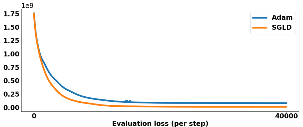
Figure 2:  The evaluation loss curve led by SGLD and Adam.

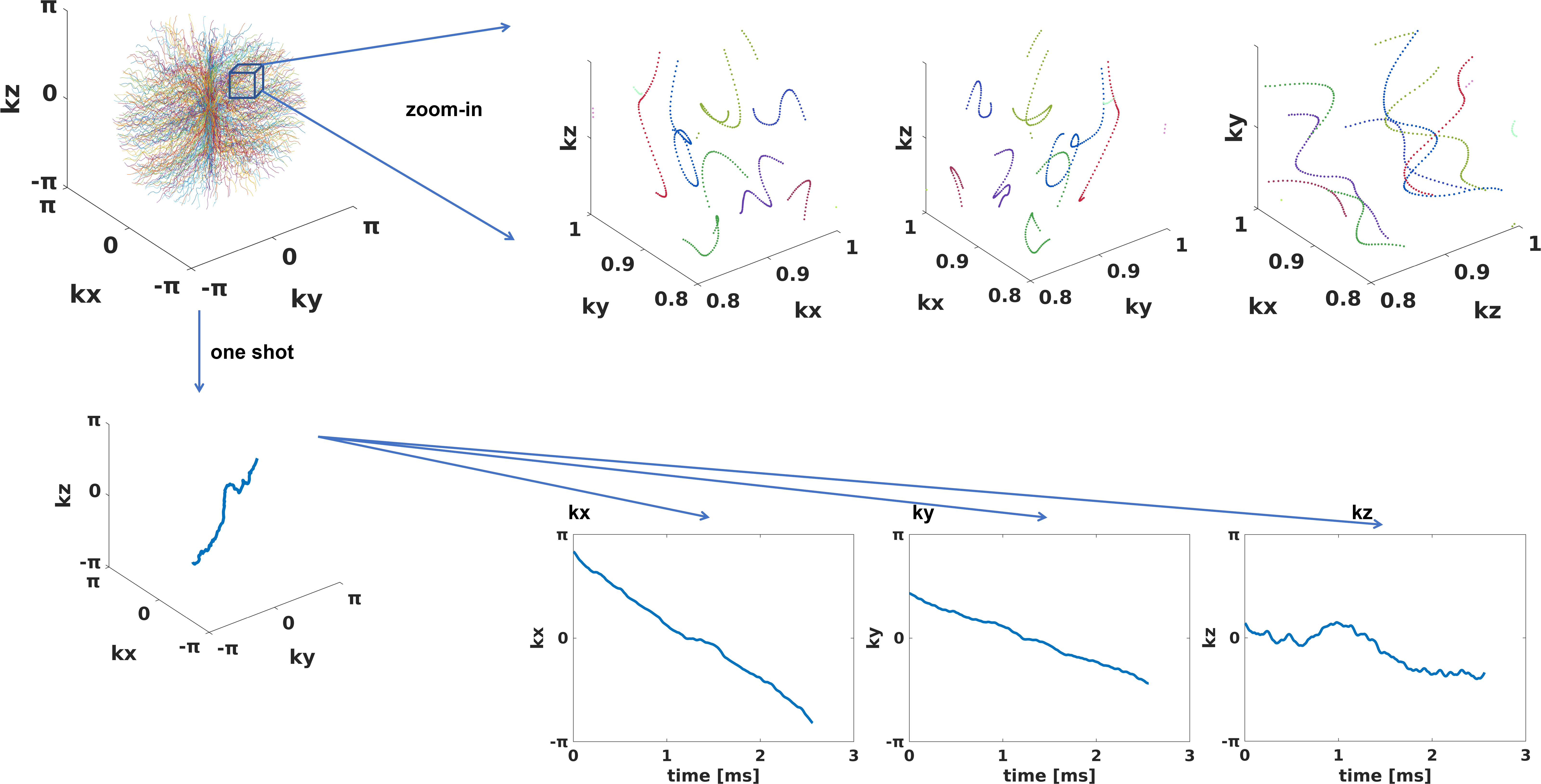
Figure 3:  The optimized sampling trajectory of experiment 7.2.1. The training involves SKM-TEA dataset and MoDL ³⁷ reconstruction. The upper row shows a zoomed-in region from different viewing perspectives. The lower row shows one shot from different perspectives.

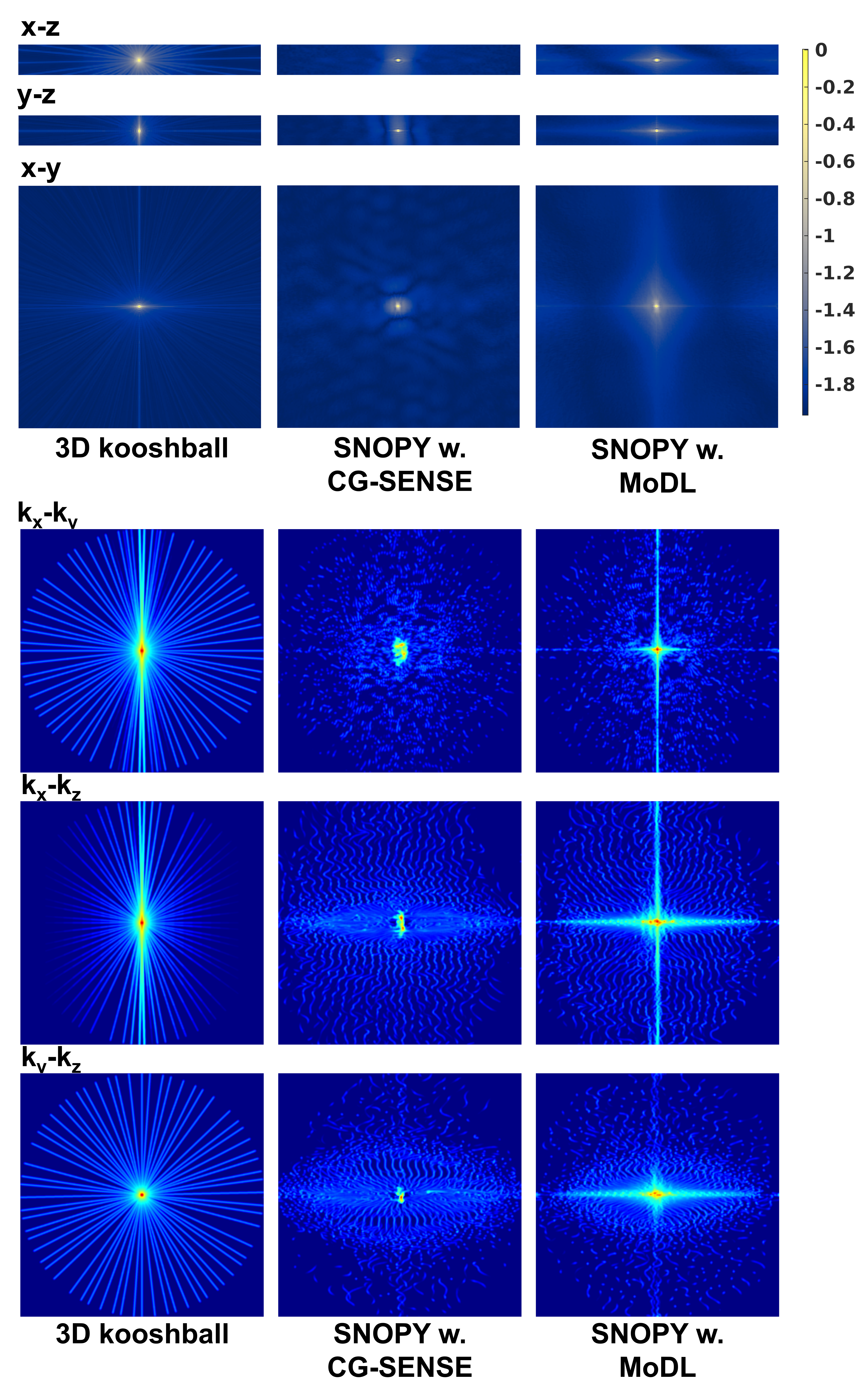
Figure 4:  Visualization of the optimized trajectory in 7.2.1. The upper subfigure displays PSFs (log-scaled, single-coil) of trajectories optimized with different reconstruction methods. The lower subfigure shows the density of sampling trajectories, by convolving the sampling points with a Gaussian kernel. Three rows are central profiles from three perspectives.

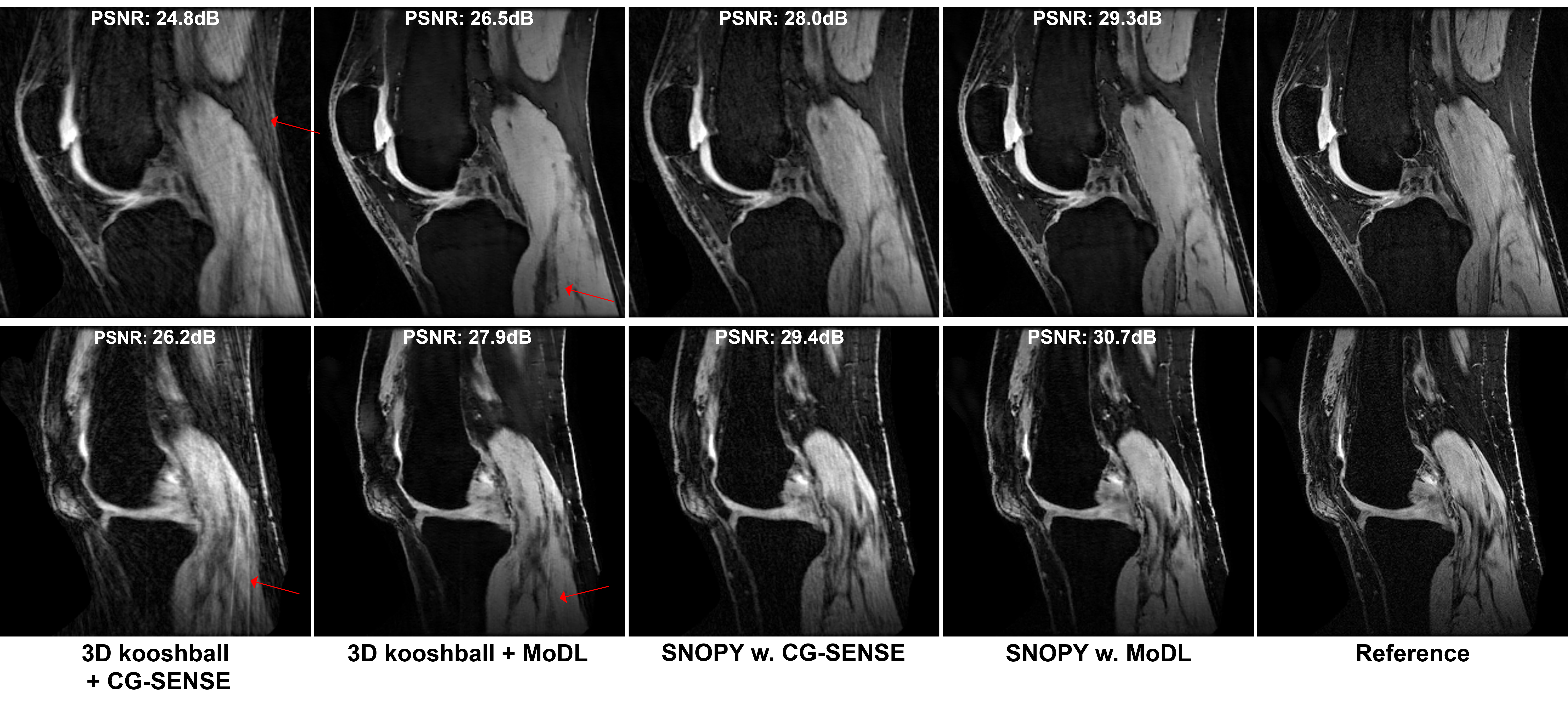
Figure 5:  Examples of the reconstructed images for two knee slices in experiment 7.2.1.

6.5.2 Memory saving techniques

Due to the large dimension, the memory cost for naive 3D trajectory optimization would be prohibitively intensive. We developed several techniques to reduce memory use and accelerate training.

As discussed above, the efficient Jacobian approximation uses only 10% of the memory used in the standard auto-differentiation approach ²⁸. We also used in-place operations in certain reconstruction steps, such as the conjugate gradient (CG) method, because with careful design it will still permit auto-differentiation. (See our open-source code for details.) The primary memory bottleneck is with the 3D NUFFT operators. We pre-calculate the Toeplitz embedding kernel to save memory and accelerate computation ^{31, 41}. In the training phase, we use a NUFFT with lower accuracy, for instance, with a smaller oversampling ratio for gridding ²⁸. Table 1 shows the incrementally improved efficiency achieved with these techniques. Without the proposed techniques, optimizing 3D trajectories would require hundreds of gigabytes of memory, which would be impractical. SNOPY enables solving this otherwise prohibitively large problem on a single graphic card (GPU).

7 Methods

7.1 Datasets

We used two publicly available datasets; both of them contain 3D multi-coil raw k-space data. SKM-TEA ⁴² is a 3D quantitative double-echo steady-state (qDESS⁴³) knee dataset. It was acquired by 3T GE MR750 scanners and 15/16-channel receiver coils. SKM-TEA includes 155 subjects. We used 132 for training, 10 for validation, and 13 for the test. Calgary brain dataset ⁴⁴ is a 3D brain T1w MP-RAGE ⁴⁵ k-space dataset. It includes 67 available subjects, acquired by an MR750 scanner and 12-channel head coils. We used 50 for training, 6 for validation, and 7 for testing. All receiver coil sensitivity maps were calculated by ESPIRiT ⁴⁶.

Table 2: The quantitative reconstruction quality (PSNR) of the test set.

	CG-SENSE	PLS	MoDL
3D kooshball	28.15 dB	28.16 dB	30.07 dB
SNOPY	32.47 dB	32.53 dB	33.68 dB

7.2 Simulation experiments

We experimented with multiple scenarios to show the broad applicability of the proposed method. All the experiments used a server node equipped with an Nvidia Tesla A40 GPU for training.

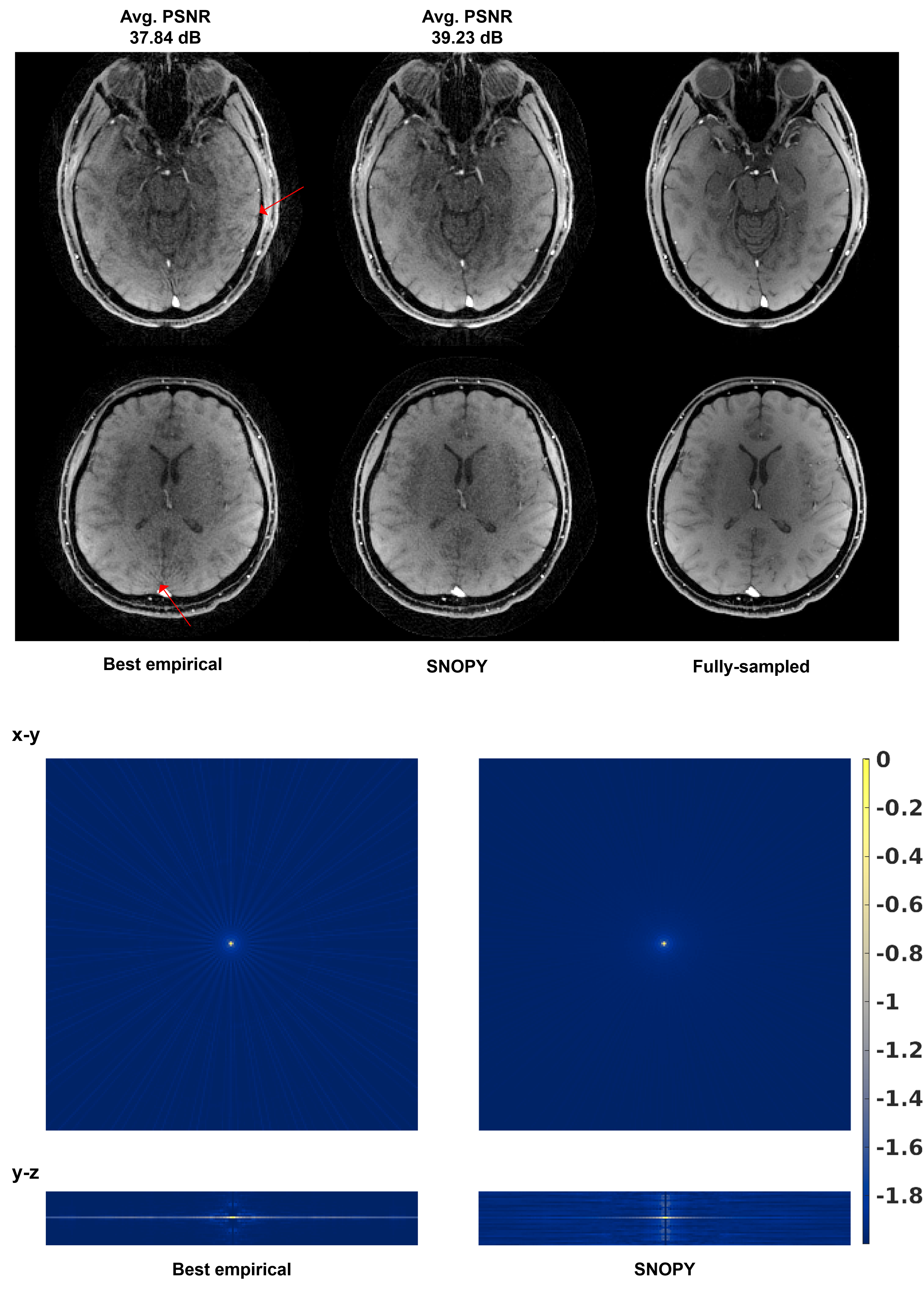
Figure 6:  Prospective results of 7.2.2, optimizing the rotation angles of the stack-of-stars (6$\times$ acceleration). ‘Best empirical’ uses the design from previous study ¹². The upper subfigure shows two slices from prospective in-vivo experiments. The reconstruction algorithm was PLS. Avg. PSNR is the average PSNR of the 4 subjects compared to the fully sampled reference. The lower subfigure shows the log-scaled PSF (single-coil) of two trajectories.

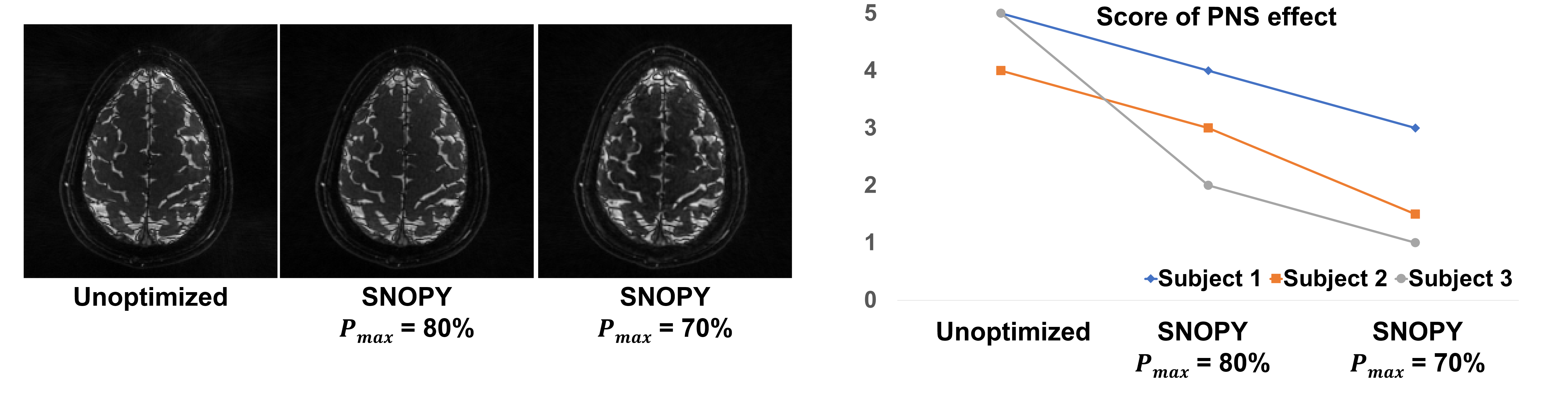
Figure 7:  Prospective results of 7.2.3. We showed three different trajectories: the unoptimized REPI, SNOPY-optimized with the PNS threshold of 80%, and SNOPY-optimized with the PNS threshold of 70%. The left subfigure shows one slice of reconstructed images. The reconstruction used PLS and 120 shots (volume TR = 2s). The right subfigure shows the subjective score of the PNS effect.

7.2.1 Optimizing 3D gradient waveform

We optimized the sampling trajectory with a 3D radial (“kooshball”) initialization ^{47, 48}. As described in 6.3, we directly optimized the readout waveform of each shot. The trajectory was parameterized by B-spline kernels to reduce the number of degrees of freedom and enable multi-scale optimization. The initial 3D radial trajectory had a 5.1 2ms readout (raster time = 4 $\mu$s) and 1024 spokes/shots (8$\times$ acceleration), using the rotation angle described in Ref. chaithya:2022:OptimizingFull3D. The training used the SKM-TEA dataset. The FOV was 15.8$\times$15.8$\times$5.1cm with 1mm³ resolution. The receiver bandwidth was $\pm$125kHz. The training loss was

$$\mathcal{L}=\mathcal{L}_{\mathrm{recon}}+0.1\mathcal{L}_{\mathrm{g}}+0.1\mathcal{L}_{\mathrm{s}}+\mathcal{L}_{\mathrm{pns}}.$$

The gradient strength ($g_{\max}$), slew rate ($s_{\max}$), and PNS threshold ($p_{\max}$) were 50 mT/m, 150 T/m/s, 80%, respectively. The learning rate $\eta_{\bm{\omega}}$ decayed from 1e-4 to 0 linearly. For the multi-level optimization, we used 3 levels (with B-spline kernel widths = 32, 16, and 8 time samples), and each level used 200 epochs. The total training time was $\sim$180 hrs. We also optimized the trajectory for several image reconstruction algorithms. We used a regularizer weight of 1e-3 and 30 CG iterations for CG-SENSE and PLS. For learning-based reconstruction, we used the MoDL ³⁷ approach that alternates between a neural network-based denoiser and data consistency updates. We used a 3D version of the denoising network ⁴⁹, 20 CG iterations for the data consistency update, and 6 outer iterations. Similar to previous investigations ^{14, 19}, SNOPY jointly optimized the neural network’s parameters and the sampling trajectories using (9).

7.2.2 Optimizing rotation angles of stack-of-stars trajectory

This experiment optimized the rotation angles of stack-of-stars, which is a widely used volumetric imaging sequence. The training used Calgary brain dataset. We used PLS as the reconstruction method for simplicity, with $\lambda=10^{-3}$ and 30 iterations. We used 200 epochs and a learning rate linearly decaying from 1e-4 to 0. The FOV is 25.6$\times$21.8$\times$3.2 cm and the resolution is 1mm³. We used 40 spokes per $kz$ location (6$\times$ acceleration), and 1280 spokes in total. The readout length is 3.5 ms. The receiver bandwidth is $\pm$125kHz. The trajectory was a stack of 32 stars, so we optimized 1280 rotation angles $\bm{c}$.

Since optimizing rotation angles does not impact the gradient strength, slew rate, PNS, and image contrast, we used only the reconstruction loss $\mathcal{L}=\mathcal{L}_{\mathrm{recon}}.$ We regard the method (RSOS-GR) proposed in previous work ¹² as the best currently available scheme. We applied 200 epochs with a linearly decaying learning rate from 1e-3 to 0. The training cost $\sim$20 hrs.

7.2.3 PNS suppression of 3D rotational EPI trajectory for functional imaging

The third application optimizes the rotation EPI (REPI) trajectory ⁵⁰, which provides an efficient sampling strategy for fMRI. For higher resolution (i.e., $\leq$1mm), we found that subjects may experience strong PNS effects introduced by REPI. This experiment aimed to reduce the PNS effect of REPI while preserving the original image contrast. We optimized one shot/readout waveform of REPI with a B-spline kernel with a width of 16 to parameterize the trajectory, and rotated the optimized readout shot using the angle scheme similar to ⁵⁰.

We designed the REPI readout for an oscillating stead steady imaging (OSSI) sequence, a novel fMRI signal model that can improve the SNR ^{51, 52}. The FOV is 20$\times$20$\times$1.2 cm, with 1 mm³ isotropic resolution, TR = 16 ms, and TE = 7.4 ms. The readout length is 10.6 ms. The receiver bandwidth is $\pm$250kHz.

To accelerate training, the loss term here excluded the reconstruction loss $\mathcal{L}_{\mathrm{recon}}$:

$$\mathcal{L}=0.01\mathcal{L}_{g}+0.01\mathcal{L}_{s}+\mathcal{L}_{pns}+\mathcal{L}_{c}.$$

The training used 40,000 steps, with a learning rate decaying linearly from 1e-4 to 0. The training cost $\sim$1 hrs.

7.3 In-vivo experiments

We implemented the optimized trajectory prospectively on a GE UHP 3.0T scanner equipped with a Nova Medical 32-channel head coil. Participants gave informed consent under local IRB approval. Because the cache in the MR system cannot load hundreds of distinct gradient waveforms, the experiment 7.2.1 was not implemented prospectively. Readers may refer to the corresponding 2D prospective studies ¹⁹ for image quality improvement and correction of eddy current effects. For experiment 7.2.2, we programmed the sampling trajectory with a 3D T1w fat-saturated GRE sequence ⁵³, with TR/TE = 14/3.2ms and FA = 20°. The experiment included 4 healthy subjects. For experiment 7.2.3, to rate the PNS effect, we asked 3 participants to score the nerve stimulation with a 5-point Likert scale from ‘mild tingling’ to ‘strong muscular twitch.’

7.4 Reproducible research

The code for 2D trajectory optimization is publicly available. As an accompanying project, MIRTorch facilitates the differentiable programming for MRI sampling and reconstruction. When this paper is accepted, we will also provide the 3D version as a toolbox on open-source platforms. For the prospective in-vivo experiments, we will provide open-source and vendor-agnostic sequences based on TOPPE ⁵³.

8 Results

For the spline-based freeform optimization experiment delineated in 7.2.1, Fig. 3 shows an example of the optimized trajectory with zoomed-in regions and plots of a single shot. Similar to the 2D case ¹⁹ and SPARKLING ^{16, 17}, the multi-level B-spline optimization leads to a swirling trajectory that can cover more k-space in the fixed readout time, to reduce large gaps between sampling locations and thus help reduce aliasing artifacts. Fig. 4 displays point spread functions (PSF) of trajectories optimized jointly with different reconstruction algorithms. To visualize the sampling density in different regions of k-space, we convolved the trajectory with a Gaussian kernel, and Fig. 4 shows the density of central profiles from different views. Compared with 3D kooshball, the SNOPY optimization led to fewer radial patterns in the PSF, corresponding to fewer streak artifacts in Fig. 5. Different reconstruction algorithms generated distinct optimized PSFs and densities, which agrees with previous studies ^{28, 54, 55}. Table 2 lists the quantitative reconstruction quality of different trajectories. The image quality metric is the average peak signal-to-noise ratio (PSNR) of the test set. SNOPY led to $\sim$4 dB higher PSNR than the kooshball initialization. Fig. 5 includes examples of reconstructed images. Compared to kooshball, SNOPY’s reconstructed images have fewer artifacts and blurring. Though MoDL reconstruction (and its variants) is one of the best reconstruction algorithms based on the open fastMRI reconstruction challenge ⁵⁶, many important structures are misplaced with the kooshball reconstruction. Using the SNOPY-optimized trajectory, even a simple model-based reconstruction (CG-SENSE) can reconstruct these structures.

For experiment 7.2.2, Fig. 6 shows the PSF of the optimized angle and RSOS-GR angle scheme ¹². For the in-plane ($x$-$y$) PSF, the SNOPY rotation shows noticeably reduced streak-like patterns. In the $y$-$z$ direction, SNOPY optimization leads to a narrower central lobe and suppressed aliasing. The prospective in-vivo experiments also support this theoretical finding. In Fig. 6, the example slices (reconstructed by PLS) from prospective studies show that SNOPY reduces streaking artifacts and blurring. The average PSNR of SNOPY and RSOS-GR for the 4 participants were 39.23 dB and 37.84 dB, respectively.

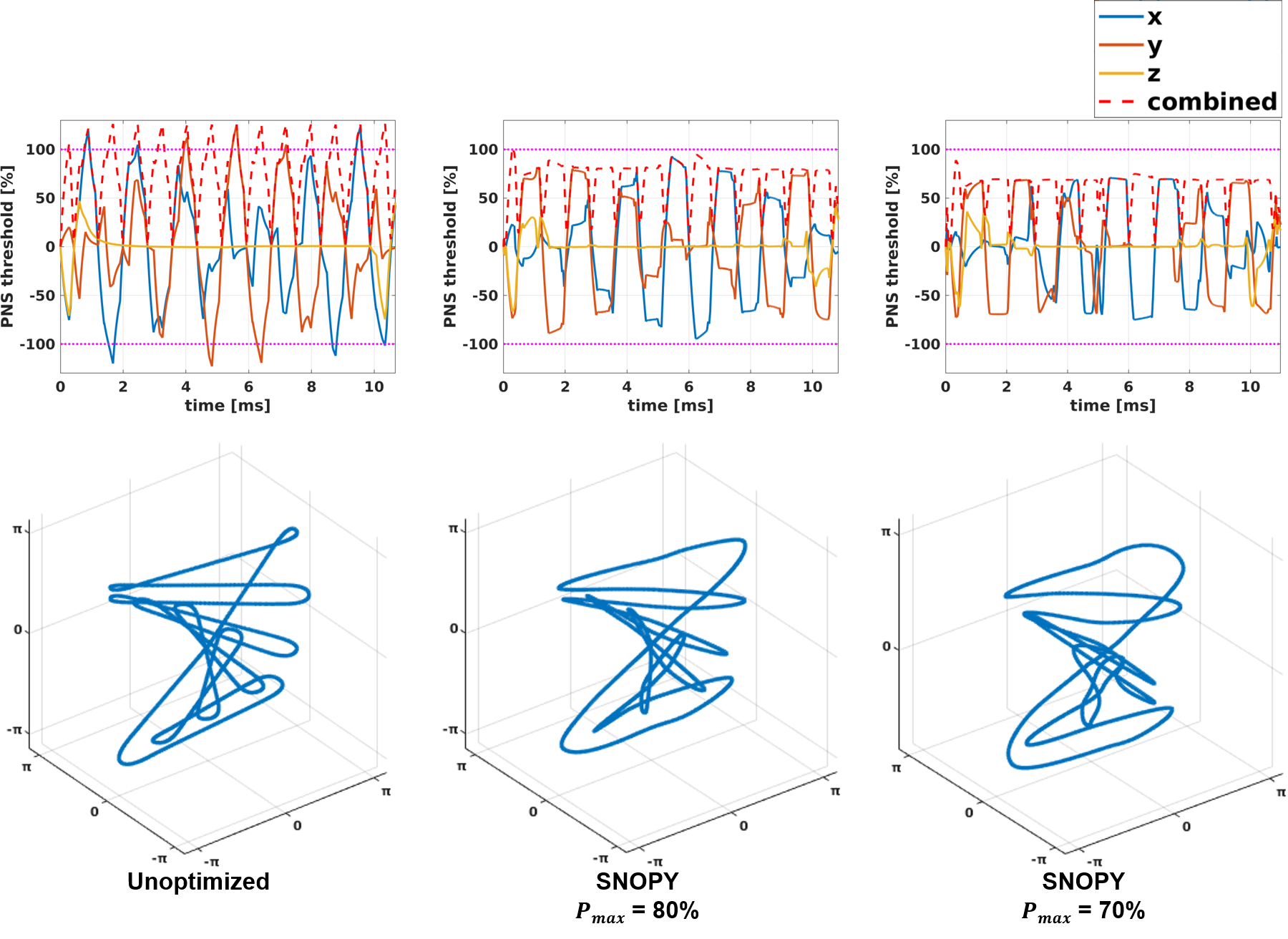
Figure 8:  The first row plots the PNS effect calculated by the convolution model (5) of the experiment 7.2.3. The second row shows one readout trajectory before/after the SNOPY optimization.

In experiment 7.2.3, we tested three settings: unoptimized REPI, optimized with PNS threshold ($p_{\max}$ in (5)) = 80%, and optimized with $p_{\max}$ = 70%. Fig. 8 shows one shot before/after the optimization, and a plot of simulated PNS effects. For the subjective rating of PNS, the first participant reported 5,2,1; the second participant reported 4,3,2; the third participant reported 5, 4, 3. The SNOPY optimization effectively reduced the subjective PNS effect of the given REPI readout in both simulation and in-vivo experiments. Intuitively, SNOPY smooths the trajectory to avoid a constantly high slew rate, preventing the high PNS effect. Fig. 7 shows one slice of reconstructed images by the CS-SENSE algorithm. Though SNOPY suppressed the PNS effect, the image contrast was well preserved by the image contrast regularizer (6).

9 Discussion

SNOPY presents a novel yet intuitive approach to optimizing non-Cartesian sampling trajectories. Via differentiable programming, SNOPY enables applying gradient-based and data-driven methods to trajectory design. Various applications and in-vivo experiments showed the applicability and robustness of SNOPY.

Experiments 7.2.1 and 7.2.2 used training data to improve image quality by trajectory optimization. SNOPY can tailor the sampling trajectory to specific training datasets and reconstruction algorithms by formulating the reconstruction image quality as a training loss. An accompanying question is whether the learned sampling trajectories could overfit the training dataset. In experiment 7.2.2, the training set used an MP-RAGE sequence, while the prospective sequence was an RF-spoiled GRE. In a 2D experiment ¹⁹, we found that trajectories learned with one anatomy (brain), contrast (T1w), and vendor (Siemens) still improved the image quality of other anatomies (like the knee), contrasts (T2w), and vendors (GE). These empirical studies indicate that trajectory optimization is robust to a moderate distribution shift between training and inference. An intuitive explanation is that SNOPY can improve the PSF by reducing the aliasing, and such improvement is universally beneficial. In subsequent investigations with more diverse datasets, we plan to study the robustness of SNOPY in more settings. For instance, one may optimize the trajectories with healthy controls and prospectively test the trajectories with pathological participants, to examine the image quality of pathologies. Testing SNOPY with different FOVs, resolutions, and field strengths will also be desirable.

An MRI system suffers from imperfections, such as field inhomogeneity ⁵⁷, eddy currents ⁵⁸, and gradient non-linearity ⁵⁹. Many correction approaches exist, such as B0-informed reconstruction ³¹ and trajectory mapping ^{60, 61}. SNOPY-optimized trajectories are compatible with these existing methods. For example, we implemented eddy-current correction for a 2D freeform optimized trajectory in Ref. wang:22:bjork-tmi. It is also possible to consider these perfections in the forward learning/optimization phase, so the optimized trajectory has innate robustness to imperfections. For instance, the forward system model $\bm{A}$ in (1) could include off-resonance maps. This prospective learning approach will require prior knowledge of the distribution of system imperfections, which is usually scanner-specific and hard to simulate. In future studies, we plan to investigate approaches to simulate such effects prospectively.

SNOPY uses a relatively simplified model of PNS. More precise models, such as Ref. davids2019prediction, may lead to improved PNS suppression results.

The training uses several loss terms, including image quality, PNS suppression, hardware limits, and image contrast. By combining these terms, the optimization can lead to trajectories that boast multiple desired characteristics. The weights of different loss terms were determined empirically. One may control the optimization results by altering the coefficients. For example, with a larger coefficient of the hardware constraint loss, the trajectory will better conform to $s_{\max}$ and $g_{\max}$. Bayesian experiment design is also applicable to finding the optimal loss weights. Additionally, the training losses (constraints) may contradict each other, and the optimization may get stuck in a local minimizer. We considered several empirical solutions to this problem. Similar to SPARKLING ¹⁷, one may relax the constraint on maximum gradient strength by using a higher receiver bandwidth. Using SGLD can also help escape the local minima because of its injected randomness. One may also use a larger B-spline kernel width to optimize the gradient waveform in the early stages of a coarse-to-fine search.

Trajectory optimization is a non-convex problem. SNOPY uses several methods, including effective Jacobian approximation, parameterization, multi-level optimization, and SGLD, to alleviate the non-convexity and lead to better optimization results. Such methods were found to be effective in this and previous studies ^{19, 28}. Initialization is also important for non-convex problems. SNOPY can take advantage of existing knowledge of MR sampling as a benign optimization initialization. For example, our experiments used the well-received golden-angle stack-of-stars and rotational EPI as optimization bases. The SNOPY algorithm can continue to improve these skillfully designed trajectories to combine the best of both stochastic optimization and researchers’ insights.

SNOPY can be extended to many applications, including dynamic and quantitative imaging. These new applications may require task-specific optimization objectives in addition to the ones described in 6.1. In particular, if the reconstruction method is not readily differentiable, such as the MR fingerprinting reconstruction based on dictionary matching ⁶², one needs to design a surrogate objective for image quality.

References

- Ahn et al. 1986 Ahn CB, Kim JH, Cho ZH. High-speed Spiral-scan Echo Planar NMR Imaging-I. IEEE Trans Med Imaging 1986 Mar;5(1):2–7.
- Lauterbur 1973 Lauterbur PC. Image Formation by Induced Local Interactions: Examples Employing Nuclear Magnetic Resonance. Nature 1973;242(5394):190–191.
- Breuer et al. 2006 Breuer FA, Blaimer M, Mueller MF, Seiberlich N, Heidemann RM, Griswold MA, et al. Controlled Aliasing in Volumetric Parallel Imaging (2D CAIPIRINHA). Magn Reson Med 2006;55(3):549–556.
- Pipe 1999 Pipe JG. Motion Correction with PROPELLER MRI: Application to Head Motion and Free-Breathing Cardiac Imaging. Magn Reson Med 1999;42(5):963–969.
- Glover and Law 2001 Glover GH, Law CS. Spiral-in/out BOLD fMRI for Increased SNR and Reduced Susceptibility Artifacts. Magn Reson Med 2001;46(3):515–522.
- Johansson et al. 2018 Johansson A, Balter J, Cao Y. Rigid-Body Motion Correction of the Liver in Image Reconstruction for Golden-Angle Stack-of-Stars DCE MRI. Magn Reson Med 2018;79(3):1345–1353.
- Yu et al. 2013 Yu MH, Lee JM, Yoon JH, Kiefer B, Han JK, Choi BI. Clinical Application of Controlled Aliasing in Parallel Imaging Results in a Higher Acceleration (CAIPIRINHA)-Volumetric Interpolated Breathhold (VIBE) Sequence for Gadoxetic Acid-Enhanced Liver MR Imaging. J Magn Reson Imaging 2013;38(5):1020–1026.
- Forbes et al. 2001 Forbes KPN, Pipe JG, Bird CR, Heiserman JE. PROPELLER MRI: Clinical Testing of a Novel Technique for Quantification and Compensation of Head Motion. J Magn Reson Imaging 2001;14(3):215–222.
- Lee et al. 2003 Lee JH, Hargreaves BA, Hu BS, Nishimura DG. Fast 3D Imaging Using Variable-density Spiral Trajectories with Applications to Limb Perfusion. Magn Reson Med 2003;50(6):1276–1285.
- Gurney et al. 2006 Gurney PT, Hargreaves BA, Nishimura DG. Design and Analysis of a Practical 3D Cones Trajectory. Magn Reson Med 2006;55(3):575–582.
- Johnson 2017 Johnson KM. Hybrid Radial-Cones Trajectory for Accelerated MRI. Magn Reson Med 2017;77(3):1068–1081.
- Zhou et al. 2017 Zhou Z, Han F, Yan L, Wang DJJ, Hu P. Golden-Ratio Rotated Stack-of-Stars Acquisition for Improved Volumetric MRI. Magn Reson Med 2017;78(6):2290–2298.
- Ham et al. 1997 Ham CLG, Engels JML, van de Wiel GT, Machielsen A. Peripheral Nerve Stimulation during MRI: Effects of High Gradient Amplitudes and Switching Rates. J Magn Reson Imaging 1997;7(5):933–937.
- Aggarwal and Jacob 2020 Aggarwal HK, Jacob M. Joint Optimization of Sampling Patterns and Deep Priors for Improved Parallel MRI. In: 2020 IEEE Intl. Conf. on Acous., Speech and Sig. Process. (ICASSP); 2020. p. 8901–8905.
- Bilgic et al. 2015 Bilgic B, et al. Wave-CAIPI for Highly Accelerated 3D Imaging. Magn Reson Med 2015;73(6):2152–2162.
- Chaithya et al. 2022 Chaithya GR, Weiss P, Daval-Frérot G, Massire A, Vignaud A, Ciuciu P. Optimizing Full 3D SPARKLING Trajectories for High-Resolution Magnetic Resonance Imaging. IEEE Trans Med Imaging 2022 Aug;41(8):2105–2117.
- Lazarus et al. 2019 Lazarus C, et al. SPARKLING: Variable-density K-space Filling Curves for Accelerated T2*-weighted MRI. Mag Res Med 2019 Jun;81(6):3643–61.
- Huijben et al. 2020 Huijben IAM, Veeling BS, van Sloun RJG. Learning Sampling and Model-based Signal Recovery for Compressed Sensing MRI. In: 2020 IEEE Intl. Conf. on Acous., Speech and Sig. Process. (ICASSP); 2020. p. 8906–8910.
- Wang et al. 2022 Wang G, Luo T, Nielsen JF, Noll DC, Fessler JA. B-Spline Parameterized Joint Optimization of Reconstruction and K-Space Trajectories (BJORK) for Accelerated 2D MRI. IEEE Trans Med Imaging 2022 Sep;41(9):2318–2330.
- Bahadir et al. 2020 Bahadir CD, Wang AQ, Dalca AV, Sabuncu MR. Deep-learning-based Optimization of the Under-sampling Pattern in MRI. IEEE Trans Comput Imag 2020;6:1139–1152.
- Weiss et al. 2021 Weiss T, Senouf O, Vedula S, Michailovich O, Zibulevsky M, Bronstein A. PILOT: Physics-Informed Learned Optimized Trajectories for Accelerated MRI. MELBA 2021;p. 1–23.
- Sanchez et al. 2020 Sanchez T, et al. Scalable Learning-based Sampling Optimization for Compressive Dynamic MRI. In: 2020 IEEE Intl. Conf. on Acous., Speech and Sig. Process. (ICASSP); 2020. p. 8584–8588.
- Jin et al. 2020 Jin KH, Unser M, Yi KM, Self-supervised Deep Active Accelerated MRI; 2020. http://arxiv.org/abs/1901.04547.
- Zeng et al. 2019 Zeng D, Sandino C, Nishimura D, Vasanawala S, Cheng J. Reinforcement Learning for Online Undersampling Pattern Optimization. In: Proc. Intl. Soc. Magn. Reson. Med. (ISMRM); 2019. p. 1092.
- Sherry et al. 2020 Sherry F, Benning M, Reyes JCD, Graves MJ, Maierhofer G, Williams G, et al. Learning the Sampling Pattern for MRI. IEEE Trans Med Imaging 2020 Dec;39(12):4310–21.
- Gözcü et al. 2018 Gözcü B, Mahabadi RK, Li YH, Ilıcak E, Çukur T, Scarlett J, et al. Learning-Based Compressive MRI. IEEE Trans Med Imaging 2018 Jun;37(6):1394–1406.
- Alush-Aben et al. 2020 Alush-Aben J, Ackerman-Schraier L, Weiss T, Vedula S, Senouf O, Bronstein A. 3D FLAT: Feasible Learned Acquisition Trajectories for Accelerated MRI. In: Deeba F, Johnson P, Würfl T, Ye JC, editors. Mach. Learn. Med. Image Reconstr. Lecture Notes in Computer Science, Cham: Springer International Publishing; 2020. p. 3–16.
- Wang and Fessler 2021 Wang G, Fessler JA, Efficient Approximation of Jacobian Matrices Involving a Non-uniform Fast Fourier Transform (NUFFT); 2021. https://arxiv.org/abs/2111.02912.
- Fessler and Sutton 2003 Fessler JA, Sutton BP. Nonuniform Fast Fourier Transforms Using Min-max Interpolation. IEEE Trans Sig Process 2003 Feb;51(2):560–74.
- Pruessmann et al. 2001 Pruessmann KP, Weiger M, Börnert P, Boesiger P. Advances in Sensitivity Encoding with Arbitrary k-space Trajectories. Magn Reson Med 2001;46(4):638–651.
- Fessler et al. 2005 Fessler JA, Lee S, Olafsson VT, Shi HR, Noll DC. Toeplitz-based Iterative Image Reconstruction for MRI with Correction for Magnetic Field Inhomogeneity. IEEE Trans Sig Process 2005 Sep;53(9):3393–402.
- Wang et al. 2004 Wang Z, Bovik AC, Sheikh HR, Simoncelli EP. Image Quality Assessment: From Error Visibility to Structural Similarity. IEEE Trans Image Process 2004 Apr;13(4):600–612.
- Schulte and Noeske 2015 Schulte RF, Noeske R. Peripheral Nerve Stimulation-Optimal Gradient Waveform Design. Magn Reson Med 2015;74(2):518–522.
- Davids et al. 2019 Davids M, Guérin B, Vom Endt A, Schad LR, Wald LL. Prediction of Peripheral Nerve Stimulation Thresholds of MRI Gradient Coils Using Coupled Electromagnetic and Neurodynamic Simulations. Magn Reson Med 2019;81(1):686–701.
- Maier et al. 2021 Maier O, et al. CG-SENSE Revisited: Results from the First ISMRM Reproducibility Challenge. Magn Reson Med 2021;85(4):1821–1839.
- Lustig et al. 2008 Lustig M, Donoho DL, Santos JM, Pauly JM. Compressed Sensing MRI. IEEE Signal Process Mag 2008 Mar;25(2):72–82.
- Aggarwal et al. 2019 Aggarwal HK, Mani MP, Jacob M. MoDL: Model-based Deep Learning Architecture for Inverse Problems. IEEE Trans Med Imaging 2019 Feb;38(2):394–405.
- Hao et al. 2016 Hao S, Fessler JA, Noll DC, Nielsen JF. Joint Design of Excitation k-Space Trajectory and RF Pulse for Small-Tip 3D Tailored Excitation in MRI. IEEE Trans Med Imaging 2016 Feb;35(2):468–479.
- Welling and Teh 2011 Welling M, Teh YW. Bayesian Learning via Stochastic Gradient Langevin Dynamics. In: Proc. 28th Int. Conf. Int. Conf. Mach. Learn (ICML). Madison, WI, USA: Omnipress; 2011. p. 681–688.
- Kingma and Ba 2017 Kingma DP, Ba J, Adam: A Method for Stochastic Optimization; 2017. http://arxiv.org/abs/1412.6980.
- Muckley et al. 2020 Muckley MJ, Stern R, Murrell T, Knoll F. TorchKbNufft: A High-Level, Hardware-Agnostic Non-Uniform Fast Fourier Transform. In: ISMRM Workshop on Data Sampling & Image Reconstruction; 2020. .
- Desai et al. 2022 Desai AD, Schmidt AM, Rubin EB, Sandino CM, Black MS, Mazzoli V, et al., SKM-TEA: A Dataset for Accelerated MRI Reconstruction with Dense Image Labels for Quantitative Clinical Evaluation; 2022. http://arxiv.org/abs/2203.06823.
- Welsch et al. 2009 Welsch GH, Scheffler K, Mamisch TC, Hughes T, Millington S, Deimling M, et al. Rapid Estimation of Cartilage T2 Based on Double Echo at Steady State (DESS) with 3 Tesla. Magn Reson Med 2009;62(2):544–549.
- Souza et al. 2018 Souza R, Lucena O, Garrafa J, Gobbi D, Saluzzi M, Appenzeller S, et al. An Open, Multi-vendor, Multi-field-strength Brain MR Dataset and Analysis of Publicly Available Skull Stripping Methods Agreement. NeuroImage 2018;170:482–494.
- Brant-Zawadzki et al. 1992 Brant-Zawadzki M, Gillan GD, Nitz WR. MP RAGE: A Three-Dimensional, T1-weighted, Gradient-Echo Sequence–Initial Experience in the Brain. Radiology 1992 Mar;182(3):769–775.
- Uecker et al. 2014 Uecker M, et al. ESPIRiT - An Eigenvalue Approach to Autocalibrating Parallel MRI: Where SENSE Meets GRAPPA. Mag Reson Med 2014 Mar;71(3):990–1001.
- Barger et al. 2002 Barger AV, Block WF, Toropov Y, Grist TM, Mistretta CA. Time-Resolved Contrast-Enhanced Imaging with Isotropic Resolution and Broad Coverage Using an Undersampled 3D Projection Trajectory. Magn Reson Med 2002;48(2):297–305.
- Herrmann et al. 2016 Herrmann KH, Krämer M, Reichenbach JR. Time Efficient 3D Radial UTE Sampling with Fully Automatic Delay Compensation on a Clinical 3T MR Scanner. PLOS ONE 2016 Mar;11(3):e0150371.
- Yu et al. 2019 Yu S, Park B, Jeong J. Deep Iterative Down-up CNN for Image Denoising. In: Proc. of the IEEE Conf. on Comput. Vis. and Patt. Recog. Work. (CVPRW); 2019. p. 0–0.
- Rettenmeier et al. 2022 Rettenmeier CA, Maziero D, Stenger VA. Three Dimensional Radial Echo Planar Imaging for Functional MRI. Magn Reson Med 2022;87(1):193–206.
- Guo and Noll 2020 Guo S, Noll DC. Oscillating Steady-State Imaging (OSSI): A Novel Method for Functional MRI. Magn Reson Med 2020;84(2):698–712.
- Guo et al. 2020 Guo S, Fessler JA, Noll DC. High-Resolution Oscillating Steady-State fMRI Using Patch-Tensor Low-Rank Reconstruction. IEEE Trans Med Imaging 2020 Dec;39(12):4357–4368.
- Nielsen and Noll 2018 Nielsen JF, Noll DC. TOPPE: a framework for rapid prototyping of MR pulse sequences. Magn Reson Med 2018;79(6):3128–3134.
- Zibetti et al. 2021 Zibetti MVW, Herman GT, Regatte RR. Fast Data-Driven Learning of Parallel MRI Sampling Patterns for Large Scale Problems. Sci Rep 2021 Sep;11(1):19312.
- Gözcü et al. 2019 Gözcü B, Sanchez T, Cevher V. Rethinking Sampling in Parallel MRI: A Data-Driven Approach. In: 2019 27th Euro. Sig. Process. Conf. (EUSIPCO); 2019. p. 1–5.
- Muckley et al. 2021 Muckley MJ, Riemenschneider B, Radmanesh A, Kim S, Jeong G, Ko J, et al. Results of the 2020 fastMRI Challenge for Machine Learning MR Image Reconstruction. IEEE Trans Med Imaging 2021 Sep;40(9):2306–2317.
- Sutton et al. 2003 Sutton BP, Noll DC, Fessler JA. Fast, Iterative Image Reconstruction for MRI in the Presence of Field Inhomogeneities. IEEE Trans Med Imaging 2003 Feb;22(2):178–188.
- Ahn and Cho 1991 Ahn CB, Cho ZH. Analysis of the Eddy-Current Induced Artifacts and the Temporal Compensation in Nuclear Magnetic Resonance Imaging. IEEE Trans Med Imaging 1991 Mar;10(1):47–52.
- Hidalgo-Tobon 2010 Hidalgo-Tobon Ss. Theory of Gradient Coil Design Methods for Magnetic Resonance Imaging. Concepts Magn Reson Part A 2010;36A(4):223–242.
- Duyn et al. 1998 Duyn JH, Yang Y, Frank JA, van der Veen JW. Simple correction method for k-space trajectory deviations in MRI. J Magn Reson 1998 May;132:150–153.
- Robison et al. 2019 Robison RK, Li Z, Wang D, Ooi MB, Pipe JG. Correction of B0 Eddy Current Effects in Spiral MRI. Magn Reson Med 2019;81(4):2501–2513.
- Ma et al. 2013 Ma D, Gulani V, Seiberlich N, Liu K, Sunshine JL, Duerk JL, et al. Magnetic Resonance Fingerprinting. Nature 2013;495(7440):187.