Eliminating artificial boundary conditions in time-dependent density functional theory using Fourier contour deformation

Abstract

We present an efficient method for propagating the time-dependent Kohn-Sham equations in free space, based on the recently introduced Fourier contour deformation (FCD) approach. For potentials which are constant outside a bounded domain, FCD yields a high-order accurate numerical solution of the time-dependent Schrödinger equation directly in free space, without the need for artificial boundary conditions. Of the many existing artificial boundary condition schemes, FCD is most similar to an exact nonlocal transparent boundary condition, but it works directly on Cartesian grids in any dimension, and runs on top of the fast Fourier transform rather than fast algorithms for the application of nonlocal history integral operators. We adapt FCD to time-dependent density functional theory (TDDFT), and describe a simple algorithm to smoothly and automatically truncate long-range Coulomb-like potentials to a time-dependent constant outside of a bounded domain of interest, so that FCD can be used. This approach eliminates errors originating from the use of artificial boundary conditions, leaving only the error of the potential truncation, which is controlled and can be systematically reduced. The method enables accurate simulations of ultrastrong nonlinear electronic processes in molecular complexes in which the inteference between bound and continuum states is of paramount importance. We demonstrate results for many-electron TDDFT calculations of absorption and strong field photoelectron spectra for one and two-dimensional models, and observe a significant reduction in the size of the computational domain required to achieve high quality results, as compared with the popular method of complex absorbing potentials.

I Introduction

Intense infrared and deep-infrared laser spectroscopy provide structural information on atomic and molecular gases which enables the inspection of ultra-fast and ultra-small-scale physics Ivanov.2021 . A variety of experimental techniques, such as high harmonic generation, photoelectron spectroscopy, and photo-fragmentation, have been used to study the nonlinear dynamics induced by strong applied fields. Experiments like these have addressed a number of fundamental questions involving, for example, the characteristic time scales of correlations Mansson.2021 , the electronic and structural changes which molecules undergo following a chemical reaction, and sub-cycle electron dynamics Trabattoni.2020 . As a consequence of their small mass, electrons are the first to respond to strong fields, and the development of theoretical and numerical methods to simulate nonlinear many-electron dynamics has underpinned tremendous progress in this field.

Simulating strong field experiments with increasingly large and complex polyatomic molecules requires the use of models capable of capturing the dynamics of many electrons interacting with the field, and accounting for interference between bound and continuum states Smirnova.2009 ; Boguslavskiy.2012 . Ab-initio approaches like time-dependent density functional theory (TDDFT), which involve no empirically fitted parameters, have become the leading approach in many-electron simulations. TDDFT reformulates the many-electron time-dependent Schrödinger equation (TDSE) as a system of nonlinear single-electron equations, coupled only through a dependence of the electronic potential on the total electron density. Electron-electron interactions are modeled using an exchange and correlation term in the potential, yielding an approximation of the full $N$-electron dynamics at the tractable cost of $N$ single-electron simulations Runge.1984 ; Marques.2011 ; Ullrich.2012 .

Numerical methods used in the electronic structure community to simulate photo-chemical processes involving ionization or scattering typically solve the underlying equations on a bounded domain of interest, and discard the outgoing part of the wavefunction. Indeed, for large scale simulations at long propagation times, it is computationally infeasible to track the full wavefunction on its entire domain of support. Instead, the true free space dynamics are mimicked using an artificial boundary scheme, which may take the form of an approximate or exact outgoing boundary condition, or an absorbing boundary layer. Even for a single electron obeying the linear time-dependent Schrödinger equation (TDSE), designing effective artificial boundaries is a challenging task, and there is an extensive literature on the subject. The available methods include complex absorbing potentials (CAPs) Navarro.2004 , mask functions (MFs) Krause.19922x ; DeGiovannini.2012 , exterior complex scaling (ECS) Simon.1979m99 ; Balslev.1971 ; Moiseyev.2011 , perfectly matched layers (PMLs) johnson21 ; antoine17 ; nissen11 ; mennemann14 ; antoine20 , local artificial boundary conditions (ABCs) engquist77 ; antoine01 ; antoine04 ; Antoine.2008 , and exact nonlocal transparent boundary conditions (TBCs) baskakov91 ; jiang04 ; jiang08 ; schadle02 ; lubich02 ; schadle06 ; han04 ; han07 ; ermolaev99 ; feshchenko11 ; feshchenko13 ; feshchenko17 ; kaye18 ; kaye20 ; ji18 ; arnold03 ; arnold12 . We refer to Refs. Antoine.2008 ; antoine17 for useful introductions to the literature, and more extensive collections of references.

The use of artificial boundaries has become popular in numerical quantum chemistry, particularly in real time time-dependent electronic structure theory Li.2020l4j . This includes, beyond TDDFT with hybrids Isborn.2007 , correlated wavefunction methods such as multi-configurational self-consistent-field (MCSCF) Sato.2013 , time-dependent configuration interaction (TD-CI) Krause.2005 , and coupled cluster (CC) Nascimento.2016 . These real time techniques are essential for simulating the non-perturbative electronic response to electric fields in the strong-field regime, including phenomena such as charge redistribution, multi-photon absorption, high-harmonic generation, and strong-field ionization, in addition to photoelectron spectroscopy, which is the focus of this paper Schlegel.2007 ; Smith.2005 ; Lopata.2013 ; Luppi.2012 ; Sissay.2016 ; Zhu.2022 ; Krause.2014 ; Krause.2014y3d ; Krause.2015 ; Suzuki.2003 ; Suzuki.2004 .

In large scale TDDFT calculations, simple local methods such as CAPs are usually favored. A CAP is a purely imaginary potential added to the system Hamiltonian, which becomes nonzero outside of a subdomain of interest. This leads to damping of the wavefunction within the support of the CAP, which we refer to as an absorbing layer. CAPs are not restricted to grid-based numerical methods and have been applied to atomic-centered basis calculations Luppi.2012 ; Sissay.2016 ; Zhu.2022 even in combination with TD-CI Krause.2014 ; Krause.2014y3d ; Krause.2015 . For good performance—that is, to successfully approximate the true free space wavefunction without an excessively large absorbing layer, which itself must be discretized by a grid—CAPs require significant tuning of their functional form, the width of the absorbing layer, and the momentum components targeted for damping. We note that the popular MF method, which imposes an explicit damping of the wavefunction at each time step, is equivalent to a particular choice of CAP to first order accuracy in the time step size DeGiovannini.2015 .

We also mention ECS Simon.1979m99 , a generalization of the older complex scaling method Balslev.1971 ; Moiseyev.2011 , which uses an analytical continuation of the Hamiltonian obtained by rotating the spatial coordinates into the complex plane outside of a subdomain of interest. This complex rotation results in exponential damping of the outgoing part of the wavefunction. Although the original goal of ECS was to investigate the energy and lifetimes of shape resonances as a static problem Whitenack.2011ce1vm ; Larsen.2013 , it has more recently been applied to the implementation of artificial boundaries for the TDSE, and is now considered part of the state of the art in strong field simulations Schneider.2020 . In particular, in infinite range ECS (irECS), an unbounded element is added to a finite element discretization of the TDSE in order to represent outgoing waves damped by an ECS transformation Scrinzi.2010 . As for CAPs, irECS requires tuning parameters which control the damping of the wavefunction. In addition, despite progress in implementing variants of irECS for grid-based methods like finite differences Weinmuller.2017 , applications so far have been limited to highly symmetric systems, like atoms and dimers, amenable to the use of polar or spherical coordinate grids Telnov.2013 ; Dujardin.2014 ; Orimo.2018 ; Zhu.2020 ; Scrinzi.2022 . These grids enable the straightforward discretization of exterior domains by an element which is unbounded in the radial coordinate, but are inefficient for the more general molecular geometries often encountered in large scale TDDFT calculations.

Recently, a new method was proposed by some of the authors which eliminates the need for artificial boundaries for the linear TDSE in the case that the potential is compactly supported, or more generally, constant outside of a bounded domain kaye22_tdse . This method, which we refer to as Fourier contour deformation (FCD), represents the wavefunction as a Fourier series of complex-frequency modes, obtained from a contour deformation of the spatial Fourier variable. Such a representation correctly captures the outgoing components of the wavefunction, to a user-controllable accuracy, without imposing artificial boundaries of any kind. Waves may even leave the computational domain and return later under the influence of an applied field, without any loss of accuracy, offering a contrast with methods like CAPs and MFs, which damp outgoing waves, and irECS, which both damps outgoing waves and amplifies incoming waves. The method has several other advantages: it is spectrally accurate in space, can be coupled to high-order accurate time stepping methods, operates naturally on Cartesian grids in any dimension, and analytically includes the influence of applied fields.

The purpose of this paper is to adapt the FCD method to realistic many-electron light-matter simulations using TDDFT with regular, real space grids. This is accomplished by first applying a smooth and controlled truncation of the long range Coulomb-like potential appearing in TDDFT to a potential which is spatially constant outside of a bounded domain of interest, and then using FCD, suitably modified for the nonlinear Kohn-Sham equations. We then demonstrate, using an implementation in the Octopus code for TDDFT Tancogne-Dejean.2020 , that such a truncation can be made without significantly affecting important physical observables, and show that our approach therefore allows for the use of smaller computational domain sizes than those obtained on a Cartesian grid using CAPs.

Our approach differs in an important way from that of most existing artificial boundary schemes. All methods, including our own, must in effect make a truncation or modification of the electrostatic potential outside a subdomain of interest, though only some do so explicitly. Indeed, no method can include the effect of a generic potential on the solution outside of the computational domain. However, this is the only approximation our method makes—specifically, we make an explicit truncation of the potential to a time-dependent constant outside the subdomain of interest, and the resulting equations are solved exactly, up to controlled discretization errors, with no further artificial boundary scheme. By contrast, even for potentials which are constant or zero outside of a bounded domain, CAPs, ECS, PMLs, and local ABCs all require a further modification of the underlying equations in order to avoid boundary reflections, necessarily introducing additional errors which can be difficult to quantify.

Exact nonlocal TBC methods share this feature with the FCD method, and can be considered its close cousins. These methods have not, however, gained widespread adoption in the context of TDDFT, because of several practical barriers. Exact nonlocal TBCs must be evaluated using specialized fast algorithms in order to avoid a rapid growth of the computational cost with the propagation time, and such algorithms, like ECS, typically rely on the use of polar or spherical coordinate grids jiang08 ; han04 ; han07 ; arnold12 . Cartesian grid-based methods which have been proposed either lack fast algorithms, leaving them computationally intractable for large scale problems feshchenko11 ; feshchenko13 ; ji18 , or rely on specific low-order spatial discretizations arnold03 ; arnold12 ; mennemann14 ; ji18 . An exception, Ref. (kaye20, , Chapter 2), is significantly more complicated than the approach described here, with no obvious advantages.

This paper is organized as follows. In Section II, we briefly review TDDFT and the time-dependent Kohn-Sham equations. In Section III, we review the FCD method, and describe our potential truncation scheme. In Section IV, we compare the method with CAPs in simulations of absorption and photoemission spectroscopy. We give concluding remarks and outline future directions of research in Section V. Appendix A suggests a particular time discretization, and gives other implementation details.

Atomic units (a.u.), with $e=\hbar=m_{e}=1$, are used throughout, unless otherwise specified.

II Time-dependent Kohn-Sham equations

TDDFT provides a systematic and computationally tractable method of simulating the many-body TDSE using a collection of single-particle nonlinear TDSEs, called the time-dependent Kohn-Sham equations (TDKSE) Runge.1984 ; Marques.2011 . The solutions $\psi_{j}(x,t)$ are called the Kohn-Sham orbitals, and represent a collection of fictitious, non-interacting electronic wavefunctions whose Slater determinant reproduces the time-dependent many-body electron density $\rho(x,t)$. The equations are nonlinearly coupled through a shared potential $V_{\text{KS}}[\rho](x,t)$, called the Kohn-Sham potential, which depends only on the density of the Kohn-Sham electrons, and not on the individual orbitals. The TDKSE for $N$ electrons in an electromagnetic field, as well as the definitions of $V_{\text{KS}}$ and $\rho$, are given as follows:

$$i\partial_{t}\psi_{j}(x,t) =\frac{1}{2}\left(-i\nabla-A(t)\right)^{2}\psi_{j}(x,t)+V_{\text{KS}}[\rho](x,t)\psi_{j}(x,t)$$ (1)

$$\psi_{j}(x,0) =\psi_{j,0}(x)$$

$$V_{\text{KS}}[\rho](x,t) =v_{\rm ion}(x,t)+v_{\rm H}[\rho](x,t)+v_{\rm xc}[\rho](x,t)$$

$$\rho(x,t) =\sum_{n=1}^{N}\lvert\psi_{j}(x,t)\rvert^{2}.$$

Here, the coupling with the external electromagnetic field is described in the velocity gauge and the long-wavelength approximation by means of a spatially uniform vector potential $A(t)$, which induces an electric field $E(t)=-\frac{dA(t)}{dt}$. A factor $1/c$, with $c$ the speed of light, has been absorbed into $A(t)$. The Kohn-Sham potential $V_{\text{KS}}[\rho](x,t)$ is divided into several parts. $v_{\rm ion}(x,t)$ is the potential due to the atomic nuclei. $v_{\rm H}[\rho](x,t)$, the Hartree potential, is the classical electrostatic potential due to a charge density $\rho$, and accounts for part of the electron-electron interaction energy. $v_{\rm xc}[\rho](x,t)$, the exchange and correlation potential, accounts for the remainder of the electron-electron interaction. Although it can be shown that there exists a choice of $v_{\rm xc}[\rho](x,t)$ such that the exact many-body electron density can be recovered from the Kohn-Sham orbitals, no systematic method exists of constructing it. However, successful proposed approximations of this term, valid for large classes of physical systems, have made TDDFT a leading framework for many-electron simulations.

We note that although there exist a variety of proposals for more accurate exchange and correlation potentials which depend not only on the electron density $\rho$, but also on the individual Kohn-Sham orbitals $\psi_{j}$ and/or currents, for simplicity we restrict our discussion here to the classical case. There is no significant barrier to extending our method to the more general setting. In addition, we focus on the case of closed-shell systems in which all orbitals are doubly occupied, but our method also applies to more sophisticated formulations involving, for instance, open shells or non-collinear spins vonBarth:1972eq .

III Eliminating artificial boundary conditions using Fourier contour deformation

We present a method to solve the TDKSE (1) in free space, $x\in\mathbb{R}^{d}$ with $d$ the spatial dimension, which avoids the problem of artificial boundary conditions. Our explanation proceeds in two steps. First, we describe the Fourier contour deformation (FCD) method kaye22_tdse for (1) in the case of a Kohn-Sham potential which is constant in space, $V_{\text{KS}}[\rho](x,t)=v(t)$ for a smooth function $v$, outside of a bounded computational domain $[-L,L]^{d}$. This method solves the equation correctly, up to discretization errors, without requiring any artificial boundary conditions, and returns the solution on $[-L,L]^{d}$. Second, we propose a simple method for truncating the long-range potentials encountered in many practical calculations to a time-dependent constant $v(t)$.

III.1 FCD for potentials which are constant outside of a bounded domain

Our discussion follows Ref. kaye22_tdse , which introduced the FCD method for the linear TDSE with compactly supported potentials. Here, we expand the discussion to include nonlinear potentials of the form in (1) which are spatially constant outside of $[-L,L]^{d}$. We give a brief review, and refer the reader to the original reference for a detailed description and analysis. We assume throughout that the initial Kohn-Sham orbitals $\psi_{j,0}(x)$ are supported in $[-L,L]^{d}$, but this assumption can be lifted in certain cases.

To simplify notation, we define $V[\rho](x,t)\equiv V_{\text{KS}}[\rho](x,t)+\frac{1}{2}\lvert A(t)\rvert^{2}$, with $\lvert\cdot\rvert$ denoting the Euclidean norm, so that the first equation in (1) becomes

$$i\partial_{t}\psi_{j}(x,t)=\left(-\frac{1}{2}\nabla^{2}+iA(t)\cdot\nabla+V[\rho](x,t)\right)\psi_{j}(x,t).$$ (2)

We note that if $V[\rho](x,t)=v(t)$ outside of $[-L,L]^{d}$, for a smooth function $v(t)$, then up to a gauge transformation, we can assume $v(t)=0$, i.e. that $V[\rho]$ is compactly supported. More specifically, we can simply solve (2) with $V[\rho](x,t)$ replaced by $V[\rho](x,t)-v(t)$, and recover the original solution as $e^{-i\int_{0}^{t}v(s)\,ds}\psi_{j}(x,t)$. We therefore assume in the following discussion that $V[\rho]$ is compactly supported. For brevity of notation, we consider the solution for a single state $\psi_{j}$, and suppress the state index $j$. We also sometimes suppress the dependence of $V$ on $\rho$, writing simply $V$, and denote the product $V[\rho](x,t)\psi(x,t)$ by $\left(V\psi\right)(x,t)$.

Taking the Fourier transform of (2) gives

$$i\partial_{t}\widehat{\psi}(\xi,t) =\left(\frac{1}{2}\lvert\xi\rvert^{2}-A(t)\cdot\xi\right)\widehat{\psi}(\xi,t)+\widehat{\left(V\psi\right)}(\xi,t)$$ (3)

$$\widehat{\psi}(\xi,0) =\widehat{\psi}_{0}(\xi),$$

where we have defined the Fourier transform as

$$\widehat{f}(\xi)\equiv\int_{\mathbb{R}^{d}}e^{-i\xi\cdot x}f(x)\,dx.$$ (4)

One could then attempt to solve (3) by a pseudospectral method, proceeding as follows:

1. Given $\widehat{\psi}(\xi,t-\Delta t)$ and $\widehat{\left(V\psi\right)}(\xi,t-\Delta t)$, take a time step of size $\Delta t$ by solving (3) to obtain $\widehat{\psi}(\xi,t)$.

2. Apply the inverse Fourier transform to obtain $\psi(x,t)$.

3. Compute $\left(V\psi\right)(x,t)$, use it to compute $\widehat{\left(V\psi\right)}(\xi,t)$, and repeat.

Since $V$ is compactly supported, such a method already appears to eliminate the problem of artificial boundary conditions. Indeed, we are only ever required to compute the Fourier transform of $\left(V\psi\right)(x,t)$, which is compactly supported, and $\psi(x,t)$ need never be evaluated outside of this support. The method does not require specifying computational domain boundaries or boundary conditions. However, as a result of the spreading of $\psi(x,t)$ over time, the number of oscillations in $\widehat{\psi}(\xi,t)$ tends to grow rapidly. Figs. 1(a)-(d) give a demonstration in the case of a Gaussian wavepacket. This limits the method to short propagation times. In particular, it can be shown that in general there is no significant difference between the number of degrees of freedom required to represent $\psi(x,t)$ on its full numerical support and that required to resolve $\widehat{\psi}(\xi,t)$ kaye22_tdse .

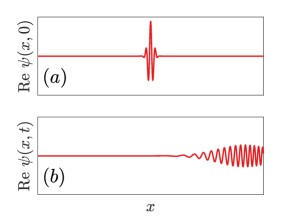
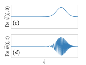
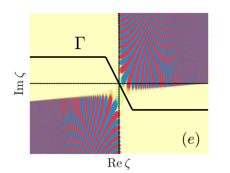
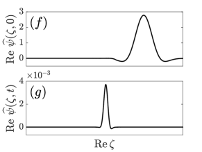
Figure 1: (a,b) A Gaussian wavepacket $\psi(x,t)$ with positive momentum, initially centered at the origin, travels rightward and spreads over time. (c,d) As a result, its Fourier transform $\widehat{\psi}(\xi,t)$ becomes more and more oscillatory; the number of oscillations in a given momentum window is proportional to $t$. (e) In the complex $\zeta$ plane, $\widehat{\psi}(\zeta,t)$ has oscillatory regions, including on the positive real axis, and non-oscillatory regions. The contour $\Gamma$ avoids the oscillatory regions. Here, $\operatorname{Re}\widehat{\psi}(\zeta,t)$ is shown on a color plot with blue indicating positive values, and red indicating negative values. (f,g) Along the contour $\zeta\in\Gamma$, the oscillations in $\widehat{\psi}(\zeta,t)$ are damped exponentially, resulting in a much smoother function than $\widehat{\psi}(\xi,t)$. Nevertheless, the wavefunction $\psi(x,t)$, restricted to the domain of interest depicted in (b), can be recovered with controllable accuracy from $\widehat{\psi}(\zeta,t)$, $\zeta\in\Gamma$. Note that the values in (f) are smaller than those in (e) because $\widehat{\psi}(\zeta,t)$ is exponentially damped along $\zeta\in\Gamma$ as $t$ increases.

To address this problem, we begin by writing $\psi(x,t)$ in terms of its inverse Fourier transform:

$$\psi(x,t)=\frac{1}{(2\pi)^{d}}\int_{\mathbb{R}^{d}}e^{i\xi\cdot x}\widehat{\psi}(\xi,t)\,d\xi.$$ (5)

In Ref. kaye22_tdse , it is shown that $\widehat{\psi}(\xi,t)$ is analytic in the entire complex plane, and the integrals in (5) can therefore be deformed to a suitable contour $\Gamma$:

$$\psi(x,t)=\frac{1}{(2\pi)^{d}}\int_{\Gamma^{d}}e^{i\zeta\cdot x}\widehat{\psi}(\zeta,t)\,d\zeta.$$ (6)

It can be shown that along the contour $\Gamma$ depicted in Figure 1(e), the oscillations in $\widehat{\psi}$ are damped exponentially, with the rate of damping proportional to the rate of oscillation. As a result, the number of degrees of freedom required to resolve $\widehat{\psi}(\zeta,t)$, for $\zeta\in\Gamma^{d}$, grows only logarithmically in time. Figs. 1(f,g) illustrate the smoothness of $\widehat{\psi}(\zeta,t)$ on $\Gamma$ for the Gaussian wavepacket example. Thus, we can simply propagate (3) by the method described above, with $\xi$ replaced by the complex contour variable $\zeta\in\Gamma^{d}$:

$$i\partial_{t}\widehat{\psi}(\zeta,t) =\left(\frac{1}{2}\zeta\cdot\zeta-A(t)\cdot\zeta\right)\widehat{\psi}(\zeta,t)+\widehat{\left(V\psi\right)}(\zeta,t)$$ (7)

$$\widehat{\psi}(\zeta,0) =\widehat{\psi}_{0}(\zeta).$$

Note that we have written $\zeta\cdot\zeta=\sum_{l=1}^{d}\zeta_{l}^{2}$ to distinguish this quantity from $\lvert\zeta\rvert^{2}=\sum_{l=1}^{d}\lvert\zeta_{l}\rvert^{2}$. We emphasize that the shape of the contour $\Gamma$ depicted in Figure 1(e) need not be hand-picked given a particular problem. Rather, this shape, which consists of two horizontal components and a diagonal component passing through the origin, is always used. The only parameter associated with $\Gamma$ is the distance from the real axis of its horizontal components, which is chosen based on a user-specified error tolerance and the “quiver radius” of the applied field, defined as $\max_{t}\lvert\int_{0}^{t}A(s)\,ds\rvert$.

Our high-order accurate implementation of the FCD method for TDDFT is described in detail in Appendix A. It involves a high-order discretization of (6), which leads to an approximation of $\psi(x,t)$, valid in $[-L,L]^{d}$, as a Fourier series with complex-frequency modes:

$$\psi(x,t)\approx\frac{1}{(2\pi)^{d}}\sum_{k=1}^{N}e^{i\zeta_{k}\cdot x}\widehat{\psi}(\zeta_{k},t)w_{k}.$$

Here, the $\zeta_{k}$ are discretization nodes on $\Gamma^{d}$, and $w_{k}$ are quadrature weights, which can be absorbed into $\widehat{\psi}(\zeta_{k},t)$ to obtain Fourier series coefficients. This gives an intuitive explanation of the FCD method: whereas for periodic problems, a Fourier series of integer modes gives an accurate representation of the wavefunction on its domain, for free space problems, a Fourier series of complex-frequency modes gives an accurate representation on $[-L,L]^{d}$.

III.2 Truncation of long-range potentials

Now that we have described a method of solving (1) for potentials $V$ which are spatially constant outside of a bounded computational domain, we must show how the potentials encountered in practical TDDFT calculations, which typically exhibit Coulomb-like decay, can be put into this form. We propose a simple method for smoothly rolling the potential off to a time-dependent constant $v(t)$ outside the sphere $S_{L}^{d-1}$ of radius $L$ centered at the origin. We take $v(t)$ to be the average of the unmodified potential over this sphere:

$$v(t)=\frac{\Gamma\left(d/2\right)}{2\pi^{d/2}L^{d-1}}\int_{S_{L}^{d-1}}V[\rho](x,t)\,dS(x).$$ (8)

For $d=1$, we define

$$v(t)=\frac{1}{2}\left(V[\rho](-L,t)+V[\rho](L,t)\right).$$

We use a partition of unity to make the transition between $V[\rho](x,t)$ and $v(t)$ smooth, thereby avoiding numerical artifacts caused by irregularities in the potential. Let $\chi:\mathbb{R}\to\mathbb{R}$ be a bump function, which is smooth and satisfies

$$\chi(x)=\begin{cases}0&\text{if }\lvert x\rvert>L\\ 1&\text{if }\lvert x\rvert<L-\sigma\end{cases}$$

for a parameter $\sigma>0$. The function

$$\chi(x)=\frac{1}{2}\left(\operatorname{erf}\left(11.6\,\frac{L-\sigma/2-x}{\sigma}\right)-\operatorname{erf}\left(11.6\,\frac{-L+\sigma/2-x}{\sigma}\right)\right)$$

satisfies these properties to within the double machine precision. For $x\in\mathbb{R}^{d}$, we can define a radial bump function by $\chi(x)\leftarrow\chi\left(\lvert x\rvert\right)$ for $x\in\mathbb{R}^{d}$. Then

$$\overline{V}[\rho](x,t)=\chi(x)V[\rho](x,t)+\left(1-\chi(x)\right)v(t)$$ (9)

is equal to $V[\rho](x,t)$ for $\lvert x\rvert<L-\sigma$, and $v(t)$ for $\lvert x\rvert>L$. The modified potential $\overline{V}[\rho]$ is therefore of the form required by the method described in the previous sections, and we propose to solve (1) with $V$ replaced by $\overline{V}$. An example of this truncation procedure, for $V$ taken to be the standard Coulomb potential, is shown in Figure 2. We note that anisotropic truncations of the potential could also be considered, and may be useful, for example, in systems with strongly polarized potentials.

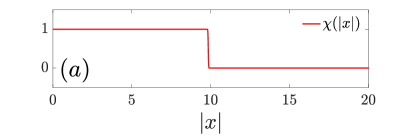
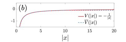
Figure 2: (a) The bump function $\chi(\lvert x\rvert)$ with $L=10$ and $\sigma=0.03L$. (b) The Coulomb potential $V(\lvert x\rvert)=-1/\lvert x\rvert$, along with its modified version, $\overline{V}(\lvert x\rvert)\equiv\chi(x)V(\lvert x\rvert)+\left(1-\chi(\lvert x\rvert)\right)V(L)$, which is consistent with (8). The modified potential $\overline{V}$ is identical to $V$ for $\lvert x\rvert<L-\sigma$ to within the double machine precision, and is smoothly truncated to the constant value $V(L)$ for $\lvert x\rvert>L$.

III.3 Summary of the method

In Section III.1, we noted that in order to apply our method, a potential equal to a constant $v(t)$ outside of $[-L,L]^{d}$ should first be reduced to a compactly supported potential by the gauge transformation $V[\rho](x,t)\leftarrow V[\rho](x,t)-v(t)$. Replacing $V$ with $\overline{V}$ in (2), making this gauge transformation, and noting that the corresponding phase shift in $\psi_{j}$ does not affect $\rho$, we obtain the following set of equations:

$$i\partial_{t}\widetilde{\psi_{j}}(x,t) =\left(-\frac{1}{2}\nabla^{2}+iA(t)\cdot\nabla+\chi(x)\left(V[\rho](x,t)-v(t)\right)\right)\widetilde{\psi_{j}}(x,t)$$ (10)

$$\widetilde{\psi_{j}}(x,0) =\widetilde{\psi_{j,0}}(x)$$

$$v(t) =\frac{\Gamma\left(d/2\right)}{2\pi^{d/2}L^{d-1}}\int_{S_{L}^{d-1}}V[\rho](x,t)\,dS(x)$$

$$\rho(x,t) =\sum_{j=1}^{N}\lvert\widetilde{\psi_{j}}(x,t)\rvert^{2}$$

$$\psi_{j}(x,t) =e^{-i\int_{0}^{t}v(s)\,ds}\widetilde{\psi_{j}}(x,t).$$

Our proposal is to solve these equations by the method described in Section III.1. In this way, by making a simple modification of the potential, we have avoided the need for artificial boundary conditions. We note that one must keep track of the indefinite integral $\int_{0}^{t}v(s)\,ds$ in order to recover $\psi_{j}$ from $\widetilde{\psi_{j}}$. This can be done using a quadrature rule of sufficiently high order to match the order of accuracy of the time discretization.

IV Numerical results: absorption and photoelectron spectra

We next present numerical results demonstrating the performance of the FCD method for TDDFT applications which require a good description of electronic excitations to continuum states. More specifically, we consider two experimentally important problems: (1) the calculation of the absorption cross section of a molecule in free space which, in the linear regime, is equivalent to the ionization cross section, and (2) the nonlinear problem of calculating the photoelectron spectrum of a molecule in the tunneling regime. We find that FCD allows us to significantly decrease the computational domain size $L$, as compared with a simulation using CAPs, while maintaining similar quality results.

The calculation of the absorption cross section in the linear regime using real time TDDFT is a standard procedure Marques.2011 ; DeGiovannini.2018 . The system is excited by including a small momentum shift in the initial condition of the Kohn-Sham orbitals, $\psi_{j,0}(x)\leftarrow e^{i\lambda\cdot x}\psi_{j,0}(x)$. The spectrum is then given by

$$S_{\alpha\beta}(\omega)=\frac{4\pi\omega}{\lambda_{\beta}}\operatorname{Im}\int_{0}^{\infty}e^{i\omega t}\left(D_{\alpha}(t)-D_{\alpha}(0)\right)\,dt,$$

where $D(t)=\int_{\mathbb{R}^{d}}x\rho(x,t)\,dx$ is the dipole moment of the electron density, and $1\leq\alpha,\beta\leq d$. In all calculations below, we take $\lambda=\lambda_{1}e_{1}$, with $e_{1}$ the unit vector aligned with the $x_{1}$ axis, and measure $S_{11}(\omega)$. We therefore make the replacement $\lambda\leftarrow\lambda_{1}$ and $S(\omega)\leftarrow S_{11}(\omega)$ for simplicity. We approximate $S$ by integrating only over a finite propagation time. The spectrum contains peaks corresponding to the allowed energy transitions of the system associated with the absorption of a photon of frequency $\omega$.

The photoelectron spectrum can be calculated using tSURFF Wopperer.2017 , a technique which has been implemented in combination with TDDFT Sato.2018rl8 ; Krecinic.2018 ; Trabattoni.2020 . The method obtains the spectrum by accumulating the momentum-projected flux of the photoionization current through a “flux surface,” which we take to be a sphere $S_{R}$ of radius $R$ enclosing the system of interest. More specifically, we first compute the momentum-resolved spectrum $P(k)=\sum_{l=1}^{N}\left|\int_{0}^{\infty}dt\,\int_{S_{R}}dS(x)\cdot j_{k,l}(x,t)\right|^{2}$, which represents the probability of measuring electrons of a given momentum vector $k$ escaping from the flux surface. Here $j_{k,l}(x,t)$ is the current density of the photoelectron corresponding to the $l^{\text{th}}$ Kohn-Sham state, projected onto Volkov waves, which are the solutions of the free particle TDSE with an applied field $A(t)$ (DeGiovannini.2018cms, , Eqs. 12, 20). In one spatial dimension, $\int_{S_{R}}dS(x)$ becomes a sum over the two points $x=\pm R$. From $P(k)$, we compute the energy-resolved spectrum, or photoelectron spectrum, by angular integration as $P(E)=\int_{|k|^{2}=2E}P(k)\,dS(k)$, which corresponds to the outgoing electron kinetic energy $E=|k|^{2}/2$. $P(E)$, which represents the probability of measuring an electron with kinetic energy $E$, is typically used to interpret the ionization process in terms of energy conservation between the electrons and the field. We refer the reader to (DeGiovannini.2018cms, , Sec. 3) for further details on the derivation of the photoelectron spectrum using tSURFF.

In simulations of both absorption and photoelectron spectroscopy, the observables can be calculated with high accuracy using only the part of the wavefunction contained in a bounded computational domain, provided that it remains free of spurious boundary reflections.

We performed all numerical experiments using the Octopus code Tancogne-Dejean.2020 , with an implementation of the FCD method. For all FCD calculations, we use the time stepping method described in Appendix A with order $p=8$, and the truncation parameter $\sigma=0.03L$. We observe that the performance is fairly insensitive to the specific choice of $\sigma$. The height of the contour $\Gamma$ is chosen according to the guidelines described in Ref. kaye22_tdse with an error tolerance $\varepsilon=10^{-8}$. For all calculations using CAPs, we use the enforced time-reversal symmetry time stepping scheme described in Ref. gomezpueyo18 , and the CAP defined in (DeGiovannini.2015, , Eq. 17) with strength parameter $\eta=-0.2$, which is chosen in order to have a wide window of energy absorption (DeGiovannini.2015, , Fig. 5). The CAP width $w$ must be adjusted to provide sufficient absorption without requiring too large of a computational domain. We emphasize that the FCD approach does not require tuning parameters like $\eta$ and $w$, so that in practice, it eliminates a costly scan over parameter space, as is required by CAPs.

In the simulations of photoemission spectroscopy, we use a vector potential of the form

$$A(t)=A_{0}\sin^{2}\left(\pi t/T\right)\cos(\omega_{0}t)\theta(T-t)\,e_{1},$$ (11)

which represents a laser pulse linearly polarized along the first coordinate direction. Here $T$ is the duration of the pulse, $A_{0}$ is the pulse strength, $\theta$ is the Heaviside function, $\omega_{0}$ is the carrier angular frequency, and $e_{1}$ is the unit vector aligned with the $x_{1}$ axis (or $e_{1}=1$ for $d=1$). The pulse strength is given by $A_{0}=\sqrt{0.28\times 10^{-16}Ic}\,/\omega_{0}$, where $I$ is the laser peak intensity in units of W/cm² (converted here to a.u.), and $c$ is the speed of light.

All calculations are converged with respect to the grid spacing $\Delta x$ and the time step $\Delta t$, and with respect to the grid spacing along the contour $\Gamma$ for FCD calculations. In this way, we focus solely on convergence with respect to the computational domain size $L$.

IV.1 One-dimensional LiH dimer

We first consider a one-dimensional model of LiH, a simple system with a nontrivial multi-electron structure containing both core and weakly-bound valence states. A majority of molecules in three dimensions present a similar energy level structure. The effective 1D Hamiltonian for the dimer is determined by an ionic potential defined as

$$v_{\rm ion}(x)=-\sum_{a=1}^{2}\frac{Z_{a}}{\sqrt{(x-X_{a})^{2}+\alpha}}.$$ (12)

Here the nuclear charge $Z_{a}$ is equal to 3 for Li and 1 for H, and $X_{1,2}=\pm 1.15$ are the centers of the two nuclei. Each is described by a soft-core potential with regularization parameter $\alpha=0.5$ a.u.² Sato.2013 . We simulate $N=4$ interacting electrons, arranged in two doubly occupied orbitals, using the one-dimensional local-density approximation (LDA) for $v_{\rm xc}$ Helbig.2011 ; Casula.2006 .

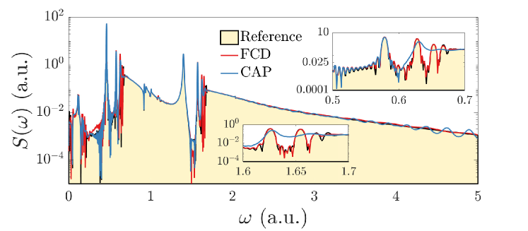
Figure 3: Computed absorption spectrum for the one-dimensional LiH example. We show results from a well-converged reference on a large domain, along with FCD, and a CAP of width $w=10$ a.u., both on domains of width $L=30$ a.u.. The insets are zooms on the first and second continuum thresholds.

In Fig. 3 we compare the absorption cross section computed with FCD, and with a CAP, on computational domains of the same size. We propagate for approximately $24$ fs, and use a momentum parameter $\lambda=0.01$ a.u. to excite the initial state. In black, we show a reference spectrum, obtained using a CAP, which was converged with respect to all simulation parameters, including the computational domain size $L$ and the CAP width $w$. Since the system has two well-separated bound states, the cross section shows two distinct ionization thresholds near $0.7$ a.u. and $1.7$ a.u., corresponding to the ionization energies of the two states. A calculation using FCD on a domain of width $L=30$ a.u. is largely successful in capturing the detailed structure of the spectrum. On the other hand, the result using a CAP of width $w=10$ a.u. on a domain of width $L=30$ a.u. is poorer, exhibiting spurious oscillations at high energies, and a discrepancy localized near the peaks corresponding to the ionization thresholds. Here $w$ was varied to achieve the best possible result, and it cannot be further improved as long as $L$ is kept fixed. In our experiments, achieving a similar quality result with a CAP required a domain of width at least $L=60$, using a CAP of width $w=20$. For both the FCD and CAP simulations, we used a converged grid spacing $\Delta x=0.3$ a.u. and time step $\Delta t\approx 0.001$ fs.

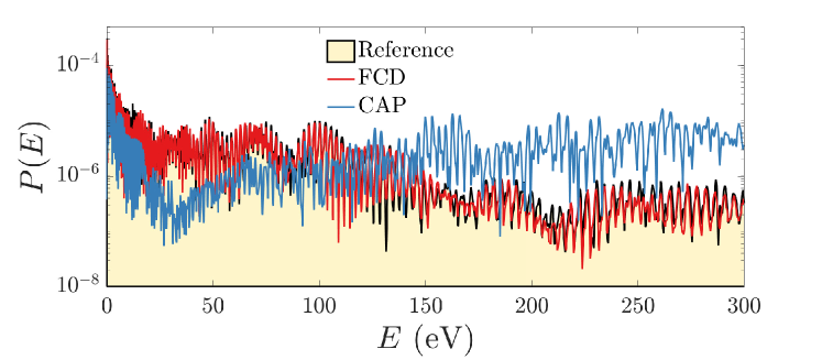
Figure 4: Computed photoemission spectrum for the one-dimensional LiH example. We show results from a well-converged reference on a large domain, along with FCD, and a CAP of width $w=10$ a.u., both on domains of width $L=50$ a.u..

We next investigate the nonlinear effects of strong field ionization. We apply a $60$ fs pulse of the form (11) with intensity $I=7.7\times 10^{13}$ W/cm² and frequency $\omega_{0}=0.954$ eV, which is sufficiently strong to turn an ionized electron back toward its parent cation once the electrons have tunneled into the continuum. We estimate the quiver radius of this field (the oscillation amplitude of a free electron subjected to the field) as $38$ a.u.. We propagate the wavefunction for $90$ fs, and place the flux surface at a radius $R=40$ a.u. from the origin. Photoelectrons emerging from direct and rescattering trajectories interfere to form the photoelectron spectrum depicted in Fig. 4. The spectrum presents characteristic features of strong field dynamics, such as oscillations mirroring the pulse frequency $\omega_{0}$, which is typical of multiphoton processes. The decay behavior of the spectrum reflects the classical approximation of rescattering dynamics. It predicts a maximum energy of electron ejection at approximately $10U_{p}$, where $U_{p}=A_{0}^{2}/4$ is the ponderomotive energy Lin.2018 . In this case, we have $U_{p}\approx 12$ eV, and observe an onset of decay in the spectrum near the expected energy. In principle, the spectrum should decay to zero from this point, but in practice the finite time of simulation yields a finite tail Morales.2016 .

In this case, using FCD on a domain of width $L=50$ is sufficient to obtain good agreement with the converged reference. Using the same domain size, we then take the largest CAP width possible, $w=10$, so that the absorbing region remains outside of the flux surface. The quality of the result is poor across all energies. Increasing the domain width to $L=120$ and using a CAP of width $w=40$ yields a result of comparable quality to the FCD calculation. Here, we used the same converged grid spacing and time step size as in the absorption spectroscopy simulation.

IV.2 Two-dimensional benzene molecule

We next consider a model of a benzene molecule given by a hexagonal arrangement of six soft-core atoms in dimension $d=2$ Ceccherini.2001o6p ; Castiglia.2015 :

$$v_{\rm ion}(x)=-\sum_{a=1}^{6}\frac{1}{\sqrt{|x-X_{a}|^{2}+\alpha}}.$$ (13)

We use the regularization parameter $\alpha=0.45$ a.u.², and atomic centers $X_{a}=\big{(}R\cos(a\pi/3),R\sin(a\pi/3)\big{)}$ with $R=2.63$ a.u.. We simulate an interacting system of $N=6$ electrons in three doubly-occupied orbitals, using two-dimensional LDA Attaccalite.2002 .

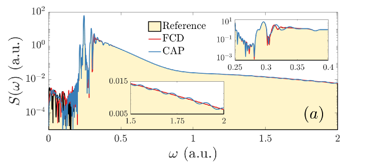
Figure 5: Computed absorption spectrum for the two-dimensional benzene example. We show results from a well-converged reference on a large domain, along with FCD, and a CAP of width $w=30$ a.u., both on domains of size $L=60$ a.u.. The insets are zooms on the continuum threshold and the high energy end of the spectrum.

The system contains a doubly degenerate HOMO state and a relatively close HOMO-1 state, as reflected by the single clean ionization threshold appearing near 0.46 a.u. in the absorption cross section shown in Fig. 5. The first ionization threshold is overshadowed by bound-to-bound transitions.

Fig. 5 compares the absorption cross section obtained using a converged reference calculation with that using FCD with a domain of size $L=60$, and a CAP of width $w=30$ on a domain of the same size ($w$ was varied to achieve the best possible result). We used a propagation time of approximately $24$ fs, and a momentum parameter $\lambda=0.01$ a.u. to excite the initial state. As in the one-dimensional example, the discrepancy is most noticeable in the large energy regime and near the ionization threshold. We note that although the spectrum should decay to zero at low energies, the finite time of propagation yields some non-zero residual, and therefore the reference calculation should not be considered to be accurate below $\omega\approx 0.2$ a.u.. A domain of size $L=140$ with a CAP of width $w=60$ was required to obtain a result of similar quality to the FCD calculation. For both the FCD and CAP simulations, we used a converged grid spacing $\Delta x=0.4$ a.u. and time step $\Delta t\approx 0.001$ fs.

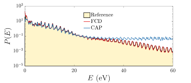
Figure 6: Angle-integrated photoemission spectrum for the two-dimensional benzene example. We show results from a well-converged reference on a large domain, along with FCD, and a CAP of width $w=10$ a.u., both on domains of size $L=50$ a.u..

Fig. 6 shows the photoelectron spectrum, obtained using a $64$ fs laser pulse with $I=10^{14}$ W/cm² and $\omega_{0}=1.55$ eV. We place the flux surface at a radius $R=40$ from the origin. We use a domain of size $L=50$ for FCD, as well as a CAP of width $w=10$ on a domain of the same size. Here, the CAP is taken to be as wide as possible while still remaining outside of the flux surface. The CAP produces a significant discrepancy with the reference calculation in the large energy regime. A domain of size $L=80$ with a CAP of width $w=40$ was required to obtain a result of similar quality to the FCD calculation. For both the FCD and CAP simulations, we used a converged grid spacing $\Delta x=0.4$ a.u. and a time step $\Delta t\approx 0.002$ fs.

An important observable which can be obtained from photoelectron experiments is the photoelectron angular distribution (PAD), which depicts the probability of measuring an electron ionized with a given momentum as a two dimensional map $P(k_{x},k_{y})$. PADs obtained by strong field ionization are commonly used to study the relationship between the electronic structure of a system and its dynamics under a strong perturbation.

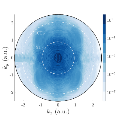
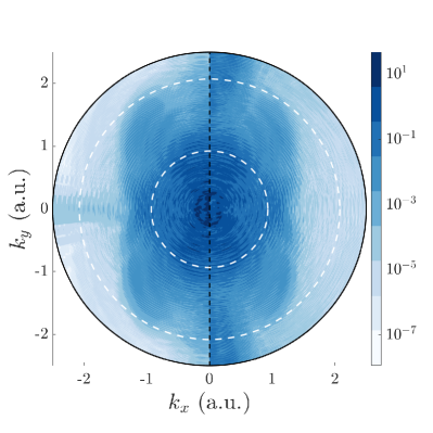
Figure 7: Photoelectron angular distribution for two-dimensional benzene example. Results for a well-converged reference are given in the left half of each plot. The FCD result on a domain of size $L=50$ a.u. is given on the right half of the first plot, and the CAP result on a domain of the same size, and a CAP width $w=10$ a.u., is given on the right half of the second plot.

Fig. 7 shows the PAD corresponding to the spectrum given in Fig. 6. It is known that photoelectrons ionized with energies below $2U_{p}$ are mostly ejected via multiphoton absorption in a process called above threshold ionization, and those with energies between $2U_{p}$ and $10U_{p}$ through rescattering processes involving a boost in kinetic energy obtained from the applied field. Considering this energy separation, several important properties of the system and its dynamics can be obtained. For instance, in the rescattering region, an intricate picture is formed by the superposition of rings centered at the value of the field at the rescattering time. From this analysis, one can infer structural properties of a system, such as its bond lengths Lin.2018 . Similarly, by analysing the “spider-leg” features formed by interference between direct and rescattered electrons, one can recover information on the time between rescattering events Huismans.2011 . A proper understanding of the details of the PAD, especially for large and complex molecules, is an active and significant area of research Wolter.2015 ; Amini.2020 ; DeGiovannini.2022 .

The comparison in Fig. 7 between the PAD obtained with FCD and with a CAP provides a much more detailed picture than Fig. 6. The main discrepancy between the reference and the CAP is concentrated along the laser polarization axis, $k_{y}$, where most of the rescattering dynamics take place. The FCD calculation, on the other hand, is in good agreement with the reference throughout the momentum domain. The low-energy regime (below $\omega\approx 1.5$ eV in Fig. 6 and $\lvert k\rvert\approx 0.33$ a.u. in Fig. 7) corresponds to photoelectrons ejected with the smallest momentum, which suffer the greatest distortion from the truncation of the Coulomb tail Arbo.2008 . Nevertheless, the FCD method reproduces the correct qualitative features of the PAD in this region much more effectively than the CAP method.

V Conclusion

We have demonstrated an implementation of the newly-introduced FCD method for TDDFT simulations in chemistry and materials science which handles the problem of spurious boundary reflections for free space problems in a different manner than standard methods like CAPs, mask functions, PMLs, and ECS. In particular, the underlying TDKSE is modified only by a smooth, controlled truncation of long range potentials, and the resulting problem is solved in a mathematically exact manner. To understand the difference with previous methods, one can consider a problem with a compactly supported potential. Whereas the methods mentioned above must still suppress boundary reflections using an absorbing boundary layer, introducing some domain truncation error, the FCD method has no such truncation error in this setting. Our approach is therefore to first reduce the TDKSE to this case, and then apply the FCD method. We find that for simulations of absorption and photoelectron spectroscopy, this yields high quality spectra with significantly smaller computational domain sizes than CAPs.

In realistic, three-dimensional TDDFT simulations using typical artificial boundary schemes, unaffordably large domains are often required to avoid excessive pollution of results by spurious boundary reflections. The FCD approach represents a promising opportunity for improvement in this respect. A scalable parallel implementation of the method in three dimensions is in progress, as well as an extension to periodic solids with one free dimension.

Appendix A High-order time propagation, and other implementation details

We suggest a particular method of high-order accurate time propagation, and leave comparison with other possible methods as an important direction of future research. The state index $j$ of $\psi_{j}$ is again made explicit in this section for clarity. We first rewrite (7) in integral form,

$$\widehat{\psi_{j}}(\zeta,t)=e^{-\frac{i}{2}\zeta\cdot\zeta t+i\zeta\cdot\varphi(t)}\widehat{\psi_{j,0}}(\zeta)-i\int_{0}^{t}e^{-\frac{i}{2}\zeta\cdot\zeta(t-s)+i\zeta\cdot(\varphi(t)-\varphi(s))}\widehat{\left(V\psi_{j}\right)}(\zeta,s)\,ds,$$ (14)

with

$$\varphi(t)\equiv\int_{0}^{t}A(s)\,ds.$$

This is simply the variation of parameters solution, treated as an ordinary differential equation for each fixed $\zeta$, with $\widehat{\left(V\psi_{j}\right)}$ considered as an inhomogeneity. Introducing a discrete time step $\Delta t$, simple algebraic manipulations allow us to eliminate the full memory dependence in (14) by writing it as a recurrence in time:

$$\widehat{\psi_{j}}(\zeta,t)=e^{-\frac{i}{2}\zeta\cdot\zeta\Delta t+i\zeta\cdot\left(\varphi(t)-\varphi(t-\Delta t)\right)}\widehat{\psi_{j}}(\zeta,t-\Delta t)-i\int_{t-\Delta t}^{t}e^{-\frac{i}{2}\zeta\cdot\zeta(t-s)+i\zeta\cdot(\varphi(t)-\varphi(s))}\widehat{\left(V\psi_{j}\right)}(\zeta,s)\,ds.$$ (15)

Thus, at each time step, we modify the solution by a damping phase factor and a local update integral.

This update integral can be discretized to high-order accuracy by the implicit Adams-Moulton multistep method. In this approach, to achieve $p^{\text{th}}$ order accuracy, the integrand is replaced by the polynomial interpolant of its values at $s=t,t-\Delta t,\ldots,t-(p-1)\Delta t$, and the resulting integrals are computed analytically. This yields an expression

$$\begin{multlined}\widehat{\psi_{j}}(\zeta,t)+i\mu_{0}\Delta t\widehat{\left(V\psi_{j}\right)}(\zeta,t)\approx e^{-\frac{i}{2}\zeta\cdot\zeta\Delta t+i\zeta\cdot\left(\varphi(t)-\varphi(t-\Delta t)\right)}\widehat{\psi_{j}}(\zeta,t-\Delta t)\\ -i\Delta t\sum_{k=1}^{p-1}\mu_{k}e^{-\frac{i}{2}\zeta\cdot\zeta k\Delta t+i\zeta\cdot(\varphi(t)-\varphi(t-k\Delta t))}\widehat{\left(V\psi_{j}\right)}(\zeta,t-k\Delta t),\end{multlined}\widehat{\psi_{j}}(\zeta,t)+i\mu_{0}\Delta t\widehat{\left(V\psi_{j}\right)}(\zeta,t)\approx e^{-\frac{i}{2}\zeta\cdot\zeta\Delta t+i\zeta\cdot\left(\varphi(t)-\varphi(t-\Delta t)\right)}\widehat{\psi_{j}}(\zeta,t-\Delta t)\\ -i\Delta t\sum_{k=1}^{p-1}\mu_{k}e^{-\frac{i}{2}\zeta\cdot\zeta k\Delta t+i\zeta\cdot(\varphi(t)-\varphi(t-k\Delta t))}\widehat{\left(V\psi_{j}\right)}(\zeta,t-k\Delta t),$$ (16)

with $\mu_{j}$ the Adams-Moulton weights. For a procedure to obtain the weights, along with tabulated weights for methods of up to eighth order, we refer the reader to Ref. (butcher16, , Chap. 24). At time $t$, the right hand side is known, and for brevity we write it as

$$\widehat{f_{j}}\left(\zeta,t-\Delta t\right)\equiv e^{-\frac{i}{2}\zeta\cdot\zeta\Delta t+i\zeta\cdot\left(\varphi(t)-\varphi(t-\Delta t)\right)}\widehat{\psi_{j}}(\zeta,t-\Delta t)\\ -i\Delta t\sum_{k=1}^{p-1}\mu_{k}e^{-\frac{i}{2}\zeta\cdot\zeta k\Delta t+i\zeta\cdot(\varphi(t)-\varphi(t-k\Delta t))}\widehat{\left(V\psi_{j}\right)}(\zeta,t-k\Delta t).$$ (17)

Taking the deformed inverse Fourier transform (6) then gives

$$\left(1+i\mu_{0}\Delta tV[\rho](x,t)\right)\psi_{j}(x,t)\approx\frac{1}{(2\pi)^{d}}\int_{\Gamma^{d}}e^{i\zeta\cdot x}\widehat{f_{j}}\left(\zeta,t-\Delta t\right)\,d\zeta\equiv f_{j}(x,t-\Delta t),$$

which can be solved for $\psi_{j}$ by pointwise division to obtain

$$\psi_{j}(x,t)\approx f_{j}(x,t-\Delta t)/\left(1+i\mu_{0}\Delta tV[\rho](x,t)\right).$$ (18)

This should be contrasted with a typical implicit time stepping method, in which taking a time step in general requires solving a linear system. It is a consequence of using the integral formulation (14) that the system is diagonal in this case. We have in (18) a nonlinear system of $N$ equations, $j=1,\ldots,N$, coupled via the density $\rho$ through the potential $V$.

A good guess for the iteration can be obtained from a $p^{\text{th}}$ order explicit Adams-Bashforth discretization of the update integral in (15), obtained by replacing the integrand with the polynomial interpolant of its values at $s=t-\Delta t,\ldots,t-p\Delta t$. Following the same steps as for the implicit Adams-Moulton discretization, we obtain the Adams-Bashforth guess

$$\begin{multlined}\widetilde{\psi_{j}}(x,t)\approx\frac{1}{(2\pi)^{d}}\int_{\Gamma^{d}}e^{i\zeta\cdot x}\widehat{g_{j}}(\zeta,t-\Delta t)\,d\zeta\equiv g_{j}(x,t-\Delta t),\end{multlined}\widetilde{\psi_{j}}(x,t)\approx\frac{1}{(2\pi)^{d}}\int_{\Gamma^{d}}e^{i\zeta\cdot x}\widehat{g_{j}}(\zeta,t-\Delta t)\,d\zeta\equiv g_{j}(x,t-\Delta t),$$ (19)

with

$$\widehat{g_{j}}(\zeta,t-\Delta t)=e^{-\frac{i}{2}\zeta\cdot\zeta\Delta t+i\zeta\cdot\left(\varphi(t)-\varphi(t-\Delta t)\right)}\widehat{\psi_{j}}(\zeta,t-\Delta t)-i\Delta t\sum_{k=1}^{p}\nu_{k}e^{-\frac{i}{2}\zeta\cdot\zeta k\Delta t+i\zeta\cdot(\varphi(t)-\varphi(t-k\Delta t))}\widehat{\left(V\psi_{j}\right)}(\zeta,t-k\Delta t),$$ (20)

for $\nu_{k}$ the Adams-Bashforth weights (butcher16, , Chap. 24).

We summarize the full numerical procedure as follows:

1. Given $\widehat{\psi_{j}}(\zeta,t-\Delta t)$ and $\widehat{\left(V\psi_{j}\right)}(\zeta,t-k\Delta t)$ for $k=1,\ldots,p$, compute $\widehat{f_{j}}(\zeta,t-\Delta t)$ and $\widehat{g_{j}}(\zeta,t-\Delta t)$ using (17) and (20), respectively, and compute $f_{j}(x,t-\Delta t)$ and $g_{j}(x,t-\Delta t)$ using the deformed inverse Fourier transform.

2. Compute $\rho$ using the $\widetilde{\psi_{j}}$ obtained from the Adams-Bashforth guess (19), and use it to compute an initial guess of $V[\rho]$.

3. Solve the nonlinear system (18) by self-consistent iteration; for a simple fixed point iteration, we would compute each $\psi_{j}$ from (18), compute an updated value of $\rho$ and of $V[\rho]$, and repeat.

4. Use the solutions $\psi_{j}$ to compute $\left(V\psi_{j}\right)(x,t)$ and take its Fourier transform to obtain $\widehat{\left(V\psi_{j}\right)}(\zeta,t)$. Then use (16) to compute $\widehat{\psi_{j}}(t)$, and advance to the next time step.

We must mention two remaining issues to complete our description of the method. First, we must accurately discretize and compute Fourier transforms between $x\in[-L,L]^{d}$ and $\zeta\in\Gamma^{d}$. Ref. kaye22_tdse describes a high-order discretization scheme and an FFT-based fast algorithm to compute these transforms efficiently. We note that the algorithm for $d>1$ can be simplified considerably compared with the prescription given there: given an implementation of the algorithm for $d=1$, one can simply use the separability of the complex-frequency discrete Fourier transform to apply it dimension by dimension.

Second, we require an initialization procedure to carry out the first $p-1$ time steps with $p^{\text{th}}$ order accuracy. For this, we again refer to Ref. kaye22_tdse , which describes a high-order Richardson extrapolation method for initialization. Briefly, this method performs a $p^{\text{th}}$ order time step by extrapolating the results of $j$ time steps of size $\Delta t/2^{j}$, for $j=0,\ldots,p/2-1$, obtained using the second order trapezoidal rule (the Adams-Moulton method for $p=2$), which does not require initialization.

References

- (1) Ivanov, M., “Concluding remarks: The age of molecular movies,” Faraday Discuss., vol. 228, pp. 622–629, 2021.
- (2) Månsson, E. P., Latini, S., Covito, F., Wanie, V., Galli, M., Perfetto, E., Stefanucci, G., Hübener, H., De Giovannini, U., Castrovilli, M. C., Trabattoni, A., Frassetto, F., Poletto, L., Greenwood, J. B., Légaré, F., Nisoli, M., Rubio, A., and Calegari, F., “Real-time observation of a correlation-driven sub 3 fs charge migration in ionised adenine,” Commun. Chem., vol. 4, no. 1, p. 73, 2021.
- (3) Trabattoni, A., Wiese, J., De Giovannini, U., Olivieri, J.-F., Mullins, T., Onvlee, J., Son, S.-K., Frusteri, B., Rubio, A., Trippel, S., and Küpper, J., “Setting the photoelectron clock through molecular alignment,” Nat. Commun., vol. 11, no. 1, p. 2546, 2020.
- (4) Smirnova, O., Mairesse, Y., Patchkovskii, S., Dudovich, N., Villeneuve, D., Corkum, P. B., and Ivanov, M. Y., “High harmonic interferometry of multi-electron dynamics in molecules,” Nature, vol. 460, pp. 972 – 977, 07 2009.
- (5) Boguslavskiy, A. E., Mikosch, J., Gijsbertsen, A., Spanner, M., Patchkovskii, S., Gador, N., Vrakking, M. J. J., and Stolow, A., “The multielectron ionization dynamics underlying attosecond strong-field spectroscopies,” Science, vol. 335, no. 6074, pp. 1336 – 1340, 2012.
- (6) Runge, E. and Gross, E. K. U., “Density-functional theory for time-dependent systems,” Phys. Rev. Lett., vol. 52, no. 12, pp. 997 – 1000, 1984.
- (7) Marques, M. A. L., Maitra, N. T., Nogueira, F., Gross, E. K. U., and Rubio, A., Fundamentals of Time-Dependent Density Functional Theory. Springer-Verlag, 2011.
- (8) Ullrich, C. A., Time-Dependent Density-Functional Theory. Oxford University Press, Oxford University Press, 2012.
- (9) Navarro, B., Mugaa, J. G., Palao, J. P., and Egusquiza, I. L., “Complex absorbing potentials,” Phys. Rep., vol. 395, no. 6, pp. 357 – 426, 2004-06.
- (10) Krause, J. L., Schafer, K. J., and Kulander, K. C., “Calculation of photoemission from atoms subject to intense laser fields,” Phys. Rev. A, vol. 45, no. 7, pp. 4998 – 5010, 1992.
- (11) De Giovannini, U., Varsano, D., Marques, M. A. L., Appel, H., Gross, E. K. U., and Rubio, A., “Ab initio angle- and energy-resolved photoelectron spectroscopy with time-dependent density-functional theory,” Phys. Rev. A, vol. 85, no. 6, p. 062515, 2012.
- (12) Simon, B., “The definition of molecular resonance curves by the method of exterior complex scaling,” Phys. Lett. A, vol. 71, no. 2-3, pp. 211–214, 1979.
- (13) Balslev, E. and Combes, J. M., “Spectral properties of many-body Schrödinger operators with dilatation-analytic interactions,” Commun. Math. Phys., vol. 22, no. 4, pp. 280 – 294, 1971-12.
- (14) Moiseyev, N., Non-Hermitian Quantum Mechanics. Cambridge University Press, 2011.
- (15) Johnson, S. G., “Notes on Perfectly Matched Layers (PMLs),” 2021. arXiv:2108.05348.
- (16) Antoine, X., Lorin, E., and Tang, Q., “A friendly review of absorbing boundary conditions and perfectly matched layers for classical and relativistic quantum waves equations,” Mol. Phys., vol. 115, no. 15–16, pp. 1861–1879, 2017.
- (17) Nissen, A. and Kreiss, G., “An optimized perfectly matched layer for the Schrödinger equation,” Commun. Comput. Phys., vol. 9, no. 1, p. 147–179, 2011.
- (18) Mennemann, J.-F. and Jüngel, A., “Perfectly matched layers versus discrete transparent boundary conditions in quantum device simulations,” J. Comput. Phys., vol. 275, pp. 1–24, 2014.
- (19) Antoine, X., Geuzaine, C., and Tang, Q., “Perfectly matched layer for computing the dynamics of nonlinear Schrödinger equations by pseudospectral methods. application to rotating Bose-Einstein condensates,” Commun. Nonlinear Sci. Numer. Simul., vol. 90, p. 105406, 2020.
- (20) Engquist, B. and Majda, A., “Absorbing boundary conditions for the numerical simulation of waves,” Math. Comput., vol. 31, no. 139, pp. 629–651, 1977.
- (21) Antoine, X. and Besse, C., “Construction, structure and asymptotic approximations of a microdifferential transparent boundary condition for the linear Schrödinger equation,” J. Math. Pures Appl., vol. 80, no. 7, pp. 701–738, 2001.
- (22) Antoine, X., Besse, C., and Mouysset, V., “Numerical schemes for the simulation of the two-dimensional Schrödinger equation using non-reflecting boundary conditions,” Math. Comput., vol. 73, no. 248, pp. 1779–1799, 2004.
- (23) Antoine, X., Arnold, A., Besse, C., Ehrhardt, M., and Schädle, A., “A review of transparent and artificial boundary conditions techniques for linear and nonlinear Schrödinger equations,” Commun. Comput. Phys., vol. 4, no. 4, pp. 729 – 796, 2008-10.
- (24) Baskakov, V. A. and Popov, A. V., “Implementation of transparent boundaries for numerical solution of the Schrödinger equation,” Wave Motion, vol. 14, no. 2, pp. 123–128, 1991.
- (25) Jiang, S. and Greengard, L., “Fast evaluation of nonreflecting boundary conditions for the Schrödinger equation in one dimension,” Comput. Math. Appl., vol. 47, no. 6, pp. 955–966, 2004.
- (26) Jiang, S. and Greengard, L., “Efficient representation of nonreflecting boundary conditions for the time-dependent Schrödinger equation in two dimensions,” Commun. Pure Appl. Math., vol. 61, no. 2, pp. 261–288, 2008.
- (27) Schädle, A., “Non-reflecting boundary conditions for the two-dimensional Schrödinger equation,” Wave Motion, vol. 35, no. 2, pp. 181–188, 2002.
- (28) Lubich, C. and Schädle, A., “Fast convolution for non–reflecting boundary conditions,” SIAM J. Sci. Comput., vol. 24, no. 1, pp. 161–182, 2002.
- (29) Schädle, A., López-Fernández, M., and Lubich, C., “Fast and oblivious convolution quadrature,” SIAM J. Sci. Comput., vol. 28, no. 2, pp. 421–438, 2006.
- (30) Han, H. and Huang, Z., “Exact artificial boundary conditions for the Schrödinger equation in ,” Commun. Math. Sci., vol. 2, no. 1, pp. 79–94, 2004.
- (31) Han, H., Yin, D., and Huang, Z., “Numerical solutions of Schrödinger equations in ,” Numer. Methods Partial Differ. Equ., vol. 23, no. 3, pp. 511–533, 2007.
- (32) Ermolaev, A. M., Puzynin, I. V., Selin, A. V., and Vinitsky, S. I., “Integral boundary conditions for the time-dependent Schrödinger equation: Atom in a laser field,” Phys. Rev. A, vol. 60, no. 6, p. 4831, 1999.
- (33) Feshchenko, R. M. and Popov, A. V., “Exact transparent boundary condition for the parabolic equation in a rectangular computational domain,” J. Opt. Soc. Am. A, vol. 28, no. 3, pp. 373–380, 2011.
- (34) Feshchenko, R. M. and Popov, A. V., “Exact transparent boundary condition for the three-dimensional Schrödinger equation in a rectangular cuboid computational domain,” Phys. Rev. E, vol. 88, no. 5, p. 053308, 2013.
- (35) Feshchenko, R. M. and Popov, A. V., “Exact transparent boundary conditions for the parabolic wave equations with linear and quadratic potentials,” Wave Motion, vol. 68, pp. 202–209, 2017.
- (36) Kaye, J. and Greengard, L., “Transparent boundary conditions for the time-dependent Schrödinger equation with a vector potential,” arXiv preprint arXiv:1812.04200, 2018.
- (37) Kaye, J., Integral equation-based numerical methods for the time-dependent Schrödinger equation. PhD thesis, Courant Institute of Mathematical Sciences, New York University, 2020.
- (38) Ji, S., Yang, Y., Pang, G., and Antoine, X., “Accurate artificial boundary conditions for the semi-discretized linear Schrödinger and heat equations on rectangular domains,” Comput. Phys. Commun., vol. 222, pp. 84–93, 2018.
- (39) Arnold, A., Ehrhardt, M., and Sofronov, I., “Discrete transparent boundary conditions for the Schrödinger equation: fast calculation, approximation and stability,” Commun. Math. Sci, vol. 1, no. 3, pp. 501–556, 2003.
- (40) Arnold, A., Ehrhardt, M., Schulte, M., and Sofronov, I., “Discrete transparent boundary conditions for the Schrödinger equation on circular domains,” Commun. Math. Sci., vol. 10, no. 3, pp. 889–916, 2012.
- (41) Li, X., Govind, N., Isborn, C., DePrince, A. E., and Lopata, K., “Real-time time-dependent electronic structure theory,” Chem. Rev., vol. 120, no. 18, pp. 9951–9993, 2020.
- (42) Isborn, C. M., Li, X., and Tully, J. C., “Time-dependent density functional theory Ehrenfest dynamics: Collisions between atomic oxygen and graphite clusters,” J. Chem. Phys., vol. 126, no. 13, pp. 134307 – 134307–7, 2007.
- (43) Sato, T. and Ishikawa, K. L., “Time-dependent complete-active-space self-consistent-field method for multielectron dynamics in intense laser fields,” Phys. Rev. A, vol. 88, no. 2, p. 023402, 2013.
- (44) Krause, P., Klamroth, T., and Saalfrank, P., “Time-dependent configuration-interaction calculations of laser-pulse-driven many-electron dynamics: Controlled dipole switching in lithium cyanide,” J. Chem. Phys., vol. 123, no. 7, p. 074105, 2005.
- (45) Nascimento, D. R. and DePrince, A. E., “Linear absorption spectra from explicitly time-dependent equation-of-motion coupled-cluster theory,” J. Chem. Theory Comput., vol. 12, no. 12, pp. 5834–5840, 2016.
- (46) Schlegel, H. B., Smith, S. M., and Li, X., “Electronic optical response of molecules in intense fields: Comparison of TD-HF, TD-CIS, and TD-CIS(D) approaches,” J. Chem. Phys., vol. 126, no. 24, p. 244110, 2007.
- (47) Smith, S. M., Li, X., Markevitch, A. N., Romanov, D. A., Levis, R. J., and Schlegel, H. B., “A numerical simulation of nonadiabatic electron excitation in the strong field regime: Linear polyenes,” J. Phys. Chem. A, vol. 109, no. 23, pp. 5176–5185, 2005.
- (48) Lopata, K. and Govind, N., “Near and above ionization electronic excitations with non-Hermitian real-time time-dependent density functional theory,” J. Chem. Theory Comput., vol. 9, no. 11, pp. 4939 – 4946, 2013.
- (49) Luppi, E. and Head-Gordon, M., “Computation of high-harmonic generation spectra of H2 and N2 in intense laser pulses using quantum chemistry methods and time-dependent density functional theory,” Mol. Phys., vol. 110, no. 9-10, pp. 909–923, 2012.
- (50) Sissay, A., Abanador, P., Mauger, F., Gaarde, M., Schafer, K. J., and Lopata, K., “Angle-dependent strong-field molecular ionization rates with tuned range-separated time-dependent density functional theory,” J. Chem. Phys., vol. 145, no. 9, p. 094105, 2016.
- (51) Zhu, Y. and Herbert, J. M., “High harmonic spectra computed using time-dependent Kohn–Sham theory with Gaussian orbitals and a complex absorbing potential,” J. Chem. Phys., vol. 156, no. 20, p. 204123, 2022.
- (52) Krause, P., Sonk, J. A., and Schlegel, H. B., “Strong field ionization rates simulated with time-dependent configuration interaction and an absorbing potential,” J. Chem. Phys., vol. 140, no. 17, p. 174113, 2014.
- (53) Krause, P. and Schlegel, H. B., “Strong-field ionization rates of linear polyenes simulated with time-dependent configuration interaction with an absorbing potential,” J. Chem. Phys., vol. 141, no. 17, p. 174104, 2014.
- (54) Krause, P. and Schlegel, H. B., “Angle-dependent ionization of small molecules by time-dependent configuration interaction and an absorbing potential,” J. Phys. Chem. Lett., vol. 6, no. 11, pp. 2140–2146, 2015.
- (55) Suzuki, M. and Mukamel, S., “Charge and bonding redistribution in octatetraene driven by a strong laser field: Time-dependent Hartree–Fock simulation,” J. Chem. Phys., vol. 119, no. 9, pp. 4722–4730, 2003.
- (56) Suzuki, M. and Mukamel, S., “Many-body effects in molecular photoionization in intense laser fields; time-dependent Hartree–Fock simulations,” J. Chem. Phys., vol. 120, no. 2, pp. 669–676, 2004.
- (57) De Giovannini, U., Larsen, A. H., Rubio, A., and Rubio, A., “Modeling electron dynamics coupled to continuum states in finite volumes with absorbing boundaries,” Eur. Phys. J. B, vol. 88, pp. 1 – 12, 03 2015.
- (58) Whitenack, D. L. and Wasserman, A., “Density functional resonance theory of unbound electronic systems,” Phys. Rev. Lett., vol. 107, no. 16, p. 163002, 2011-10.
- (59) Larsen, A. H., Whitenack, D. L., Giovannini, U. D., Wasserman, A., and Rubio, A., “Stark ionization of atoms and molecules within density functional resonance theory,” J. Phys. Chem. Lett., vol. 4, no. 16, pp. 2734 – 2738, 2013.
- (60) Schneider, B. I. and Gharibnejad, H., “Numerical methods every atomic and molecular theorist should know,” Nat. Rev. Phys., vol. 2, no. 2, pp. 89–102, 2020.
- (61) Scrinzi, A., “Infinite-range exterior complex scaling as a perfect absorber in time-dependent problems,” Phys. Rev. A, vol. 81, no. 5, p. 053845, 2010.
- (62) Weinmüller, M., Weinmüller, M., Rohland, J., and Scrinzi, A., “Perfect absorption in Schrödinger-like problems using non-equidistant complex grids,” J. Comput. Phys., vol. 333, pp. 199 – 211, 2017.
- (63) Telnov, D. A., Sosnova, K. E., Rozenbaum, E., and Chu, S.-I., “Exterior complex scaling method in time-dependent density-functional theory: Multiphoton ionization and high-order-harmonic generation of Ar atoms,” Phys. Rev. A, vol. 87, no. 5, p. 053406, 2013.
- (64) Dujardin, J., Saenz, A., and Schlagheck, P., “A study of one-dimensional transport of Bose–Einstein condensates using exterior complex scaling,” Appl. Phys. B, vol. 117, no. 3, pp. 765–773, 2014.
- (65) Orimo, Y., Sato, T., Scrinzi, A., and Ishikawa, K. L., “Implementation of the infinite-range exterior complex scaling to the time-dependent complete-active-space self-consistent-field method,” Phys. Rev. A, vol. 97, no. 2, p. 023423, 2018.
- (66) Zhu, J., “Quantum simulation of dissociative ionization of in full dimensionality with a time-dependent surface-flux method,” Phys. Rev. A, vol. 102, no. 5, p. 053109, 2020.
- (67) Scrinzi, A., “tRecX — An environment for solving time-dependent Schrödinger-like problems,” Comput. Phys. Commun., vol. 270, p. 108146, 2022.
- (68) Kaye, J., Barnett, A., and Greengard, L., “A high-order integral equation-based solver for the time-dependent Schrödinger equation,” Commun. Pure Appl. Math., vol. 75, no. 8, pp. 1657–1712, 2022.
- (69) Tancogne-Dejean, N., Oliveira, M. J. T., Andrade, X., Appel, H., Borca, C. H., Breton, G. L., Buchholz, F., Castro, A., Corni, S., Correa, A. A., Giovannini, U. D., Delgado, A., Eich, F. G., Flick, J., Gil, G., Gomez, A., Helbig, N., Hübener, H., Jestädt, R., Jornet-Somoza, J., Larsen, A. H., Lebedeva, I. V., Lüders, M., Marques, M. A. L., Ohlmann, S. T., Pipolo, S., Rampp, M., Rozzi, C. A., Strubbe, D. A., Sato, S. A., Schäfer, C., Theophilou, I., Welden, A., and Rubio, A., “Octopus, a computational framework for exploring light-driven phenomena and quantum dynamics in extended and finite systems,” J. Chem. Phys., vol. 152, no. 12, p. 124119, 2020.
- (70) von Barth, U. and Hedin, L., “A local exchange-correlation potential for the spin polarized case: I,” J. Phys. C Solid State Phys., vol. 5, no. 13, p. 1629, 1972.
- (71) De Giovannini, U. and Castro, A., “Chapter 12: Real-time and real-space time-dependent density-functional theory approach to attosecond dynamics,” in Attosecond Molecular Dynamics (Vrakking, M. J. J. and Lepine, F., eds.), pp. 424–461, The Royal Society of Chemistry, 2019.
- (72) Wopperer, P., De Giovannini, U., and Rubio, A., “Efficient and accurate modeling of electron photoemission in nanostructures with TDDFT,” Eur. Phys. J. B, vol. 90, no. 3, p. 1307, 2017.
- (73) Sato, S. A., Hübener, H., Rubio, A., and De Giovannini, U., “First-principles simulations for attosecond photoelectron spectroscopy based on time-dependent density functional theory,” Eur. Phys. J. B, vol. 91, no. 6, p. 126, 2018.
- (74) Krečinić, F., Wopperer, P., Frusteri, B., Brauße, F., Brisset, J.-G., De Giovannini, U., Rubio, A., Rouzée, A., and Vrakking, M. J. J., “Multiple-orbital effects in laser-induced electron diffraction of aligned molecules,” Phys. Rev. A, vol. 98, no. 4, p. 041401, 2018.
- (75) De Giovannini, U., “Pump-probe photoelectron spectra,” in Handbook of Materials Modeling : Methods: Theory and Modeling (Andreoni, W. and Yip, S., eds.), pp. 1–19, Cham: Springer International Publishing, 2018.
- (76) Gómez Pueyo, A., Marques, M. A. L., Rubio, A., and Castro, A., “Propagators for the time-dependent Kohn–Sham equations: Multistep, Runge–Kutta, exponential Runge–Kutta, and commutator free Magnus methods,” J. Chem. Theory Comput., vol. 14, no. 6, pp. 3040–3052, 2018.
- (77) Helbig, N., Casula, M., Verstraete, M., Marques, M. A. L., Tokatly, I. V., and Rubio, A., “Density functional theory beyond the linear regime: Validating an adiabatic local density approximation,” Phys. Rev. A, vol. 83, no. 3, p. 032503, 2011-03.
- (78) Casula, M., Sorella, S., and Senatore, G., “Ground state properties of the one-dimensional Coulomb gas using the lattice regularized diffusion Monte Carlo method,” Phys. Rev. B, vol. 74, no. 24, p. 245427, 2006-12.
- (79) Lin, C. D., Le, A.-T., Jin, C., and Wei, H., “Elements of the quantitative rescattering theory,” J. Phys. B, vol. 51, no. 10, p. 104001, 2018.
- (80) Morales, F., Bredtmann, T., and Patchkovskii, S., “iSURF: a family of infinite-time surface flux methods,” J. Phys. B, vol. 49, no. 24, p. 245001, 2016.
- (81) Ceccherini, F. and Bauer, D., “Harmonic generation in ring-shaped molecules,” Phys. Rev. A, vol. 64, no. 3, p. 033423, 2001.
- (82) Castiglia, G., Corso, P. P., Corso, P. P., De Giovannini, U., Fiordilino, E., Fiordilino, E., Frusteri, B., and Frusteri, B., “Laser driven structured quantum rings,” J. Phys. B, vol. 48, no. 11, p. 115401, 2015.
- (83) Attaccalite, C., Moroni, S., Gori-Giorgi, P., and Bachelet, G. B., “Correlation energy and spin polarization in the 2D electron gas,” Phys. Rev. Lett., vol. 88, no. 25, p. 256601, 2002.
- (84) Huismans, Y., Smirnova, O., Rouzee, A., Gijsbertsen, A., Jungmann, J. H., Smolkowska, A. S., Logman, P. S. W. M., Lépine, F., Cauchy, C., Zamith, S., Marchenko, T., Bakker, J. M., Berden, G., Redlich, B., Meer, A. F. G. v. d., Muller, H. G., Vermin, W., Schafer, K. J., Spanner, M., Ivanov, M. Y., Bauer, D., Popruzhenko, S. V., and Vrakking, M. J. J., “Time-resolved holography with photoelectrons,” Science, vol. 331, no. 6013, pp. 61 – 64, 2011.
- (85) Wolter, B., Pullen, M. G., Baudisch, M., Sclafani, M., Hemmer, M., Senftleben, A., Schröter, C. D., Ullrich, J., Moshammer, R., and Biegert, J., “Strong-field physics with mid-IR fields,” Phys. Rev. X, vol. 5, p. 021034, 2015.
- (86) Amini, K. and Biegert, J., “Ultrafast electron diffraction imaging of gas-phase molecules,” vol. 69 of Advances In Atomic, Molecular, and Optical Physics, ch. 3, pp. 163–231, Academic Press, 2020.
- (87) De Giovannini, U., Küpper, J., and Trabattoni, A., “New perspectives in time-resolved laser-induced electron diffraction,” J. Phys. B, 2022.
- (88) Arbó, D. G., Miraglia, J., Gravielle, M., Schiessl, K., Persson, E., and Burgdörfer, J., “Coulomb-Volkov approximation for near-threshold ionization by short laser pulses,” Phys. Rev. A, vol. 77, no. 1, p. 013401, 2008-01.
- (89) Butcher, J., Numerical Methods for Ordinary Differential Equations. Wiley, 2016.