Structure Guided Manifolds for Discovery of Disease Characteristics

Abstract

In medical image analysis, the subtle visual characteristics of many diseases are challenging to discern, particularly due to the lack of paired data. For example, in mild Alzheimer’s Disease (AD), brain tissue atrophy can be difficult to observe from pure imaging data, especially without paired AD and Cognitively Normal (CN) data for comparison. This work presents Disease Discovery GAN (DiDiGAN), a weakly-supervised style-based framework for discovering and visualising subtle disease features. DiDiGAN learns a disease manifold of AD and CN visual characteristics, and the style codes sampled from this manifold are imposed onto an anatomical structural “blueprint" to synthesise paired AD and CN magnetic resonance images. To suppress non-disease related variations between the generated AD and CN pairs, DiDiGAN leverages a structural constraint with cycle consistency and anti-aliasing to enforce anatomical correspondence. When tested on the Alzheimer’s Disease Neuroimaging Initiative (ADNI) dataset, DiDiGAN showed key AD characteristics (reduced hippocampal volume, ventricular enlargement, and atrophy of cortical structures) through synthesising paired AD and CN scans. The qualitative results were backed up by automated brain volume analysis, where systematic pair-wise reductions in brain tissue structures were also measured.

I Introduction

Discovering the visual characteristics of disease states from medical imaging data can provide important insights into the presence, progression and effects of pathological changes. In many brain pathologies, magnetic resonance (MR) images provide excellent visual characterization of lesions [1] although visualizing very early or subtle changes in brain volume in conditions such as AD can be extremely challenging. Subtle AD features are difficult to discern and visualise due to the lack of paired AD and CN data to provide anatomical correspondence. Hence, experts need to know what to specifically look for. With differentiable vision systems like Convolutional Neural Networks, it is possible to automatically extract some brain features with methods like GradCAM [2]. However, GradCAM does not communicate any specific visual characteristics beyond rough locations of abnormalities. In many cases, the specific effects of a disease still require side-by-side comparisons to observe.

In theory, Generative Adversarial Networks [3] are capable of creating synthetic medical images of an anatomical structure in different disease conditions. Style-based [4][5] GANs are of particular interest for such tasks as they provide mechanisms for maintaining anatomical correspondence. The generator learns a high-dimensional latent space where style codes are sampled and then injected into the generator to manipulate the output image. It was shown that the learnt latent space forms a smooth high-dimensional manifold that facilitates image interpolation [4]. Hence, style-based GANs have been linked toc manifold and latent representation learning [6], [7]. Subsequent works, including StarGANs [8][9] demonstrated unpaired image translation using StyleGAN. It was shown that the learnt manifold (style) could be separated to govern only a select subset of features, leaving the rest of the content intact. This idea has also been demonstrated for medical image analysis [10], where (medical imaging) modality information was successfully separated from anatomical information. These works suggest style-based GANs could indeed learn a manifold of AD features to synthesise paired AD and CN scans. However, as will be shown in this paper, simply applying these methods does not produce usable synthetic AD and CN samples with sufficient anatomical correspondence (AD features, if any, are concealed by non-AD structural variations between the sample pairs).

The inability of style-based GANs to maintain anatomical correspondence can be attributed to aliasing, which is a substantive problem often overlooked in deep learning. Recently, it was reported that anti-aliasing could improve the accuracy and generalisation of CNNs [11] for classification. There have been similar findings in generative modelling. The highlight of StyleGAN3 [12] was the introduction of anti-aliasing, which mitigates “texture sticking" artifacts during latent space interpolation. While these artifacts do not significantly deteriorate image quality, they invalidate applications requiring smooth manifold interpolation. Once anti-aliasing was implemented following the Shannon-Nyquist sampling theorem [13], traversing the manifold of StyleGAN3 yields more natural transitions in the image space. This work recognises the unique aspects of anti-aliasing for establishing a reliable pair-wise anatomical correspondence. Even small artifacts in the feature maps can morph into significantly dissimilar anatomical structures. Therefore the aliasing issue must be addressed.

This current work presents DiDiGAN, a style-based network capable of synthesising paired AD and CN MR images while maintaining anatomical correspondence. Many key AD features are made observable even to the untrained eye by simple visual comparison of the generated image pairs. The highlights of this network include

• A learnt disease manifold that encodes AD and CN characteristics. The manifold is then injected into the generator to control the expression of AD features (or the lack thereof) in the output.

• The generative process is guided by a structural constraint. The constraint is low-resolution by design to establish high-level anatomical correspondence between the generated AD and CN image pairs. Its lack of fine details also leaves sufficient room for AD characteristics (style) to be synthesised. The constraint is enforced using cycle consistency.

• The first to employ anti-aliasing to enforce structural correspondence (further to the above constraint) between generated image pairs.

• The disease manifold is automatically built in a weakly supervised manner where only disease class labels are required.

DiDiGAN was tested on the ADNI dataset, where it synthesised paired AD and CN MR images. The generated image pairs clearly exhibit key AD characteristics including, reduced hippocampal volume, ventricular enlargement and cortical atrophy while maintaining pair-wise anatomical correspondence. The results were first examined by three clinical experts followed by Jacobian index analysis and brain volume analysis where systematic brain shrinkage was measured.

II Methods

The idea formulation of DiDiGAN revolves around projecting a learnt disease manifold onto a shared anatomical “blueprint" to synthesise comparable AD and CN images. This section describes the components of DiDiGAN and the mechanisms employed to synthesise disease characteristics without compromising anatomical correspondence.

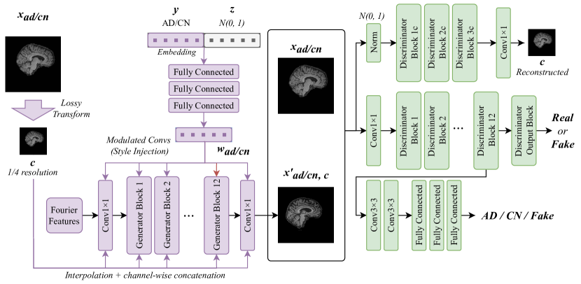
Figure 1: Architecture of DiDiGAN. The alias-free generator is conditioned on both the constraint $c$ and the disease class label $y$. The discriminator attempts to recover the input $c$ and $y$ through adversarial training.

The architecture of DiDiGAN is shown in Figure 1. The procedure to generate a pair of contrasting samples $x_{c}^{\prime}\in\{x^{\prime}_{ad,c},x^{\prime}_{cn,c}\}$ is described by $x_{ad,c}^{\prime}=G(w_{ad},c,z),\ x_{cn,c}^{\prime}=G(w_{cn},c,z)$, where

• $w\in\{w_{ad},w_{cn}\}$ are 512-d disease style codes sampled from the learnt disease manifold, in this case, AD or the lack thereof (CN). $w_{ad}$ and $w_{cn}$ are conditioned on the embeddings of the class labels $y_{ad}$ and $y_{cn}$, respectively. Each embedding is concatenated with a noise vector $z$ (for diverse outputs) and mapped to $w$ using three fully connected layers of 512 units. $w$ is injected into $G$ as style such that the generated images can reflect AD characteristics.

• $c$ is a deliberately lossy representation of an input image $x$ which acts as a rough “blueprint" for $x_{ad,c}^{\prime}$ and $x_{cn,c}^{\prime}$ to be structurally similar at a high-level. Its vagueness deliberately leaves room for specific disease characteristics (AD or CN) to be incorporated through style injection. An overly precise constraint would exert too much control over the content, diminishing disease style codes’ effect. In the present work, $c$ is simply a low-resolution version of $x$ (scaled with anti-aliasing). The scaling factor is a hyper-parameter controlling the amount of room left for AD features to develop. It was also found that other lossy representations such as segmentation maps and edge maps would also work as alternative constraints.

• $G$ is an alias-free convolutional generator with a starting resolution of $4\times 4$ and an output resolution of $256\times 256$. There are 12 convolutional blocks that gradually up-samples the image. $w$ is incorporated via modulated convolution and $c$ is imposed by channel-wise concatenation (after re-scaling as needed). While the constraint $c$ establishes high-level anatomical correspondence, anti-aliasing plays a crucial role in suppressing more fine-grained undesirable variations between $x^{\prime}_{ad,c}$ and $x^{\prime}_{cn,c}$ which are not controlled by $c$. All the operations in the generator are made alias-free following Shannon-Nyquist sample theorem, and the anti-aliasing procedures involve (or approximate) I) casting the discrete signals to the continuous domain followed by II) low-pass filtering and then III) discrete sampling back to discrete domain [12]. The key here is all the undesirable high-frequency signals in the feature space are eliminated to ensure no disruptions to anatomical correspondence.

The discriminator is a CNN with three prediction heads $D_{adv}$, $D_{C}$ and $D_{W}$, which predict I) the logit for realness, II) the reconstructed structural constraint and III) the classification of disease, non-disease or fake, respectively. These prediction heads correspond to three optimisation objectives $L_{adv}$, $L_{C}$ $L_{W}$.

$$\min_{{D}}\max_{{G}}L_{adv}=\mathbb{E}[\textnormal{log}D_{adv}(x)]\leavevmode\nobreak\ -\leavevmode\nobreak\ \mathbb{E}[\textnormal{log}(D_{adv}(x^{\prime}_{c}))]$$

$$\min_{{D}}\min_{{G}}L_{C}=||c-D_{C}(x^{\prime}_{c})||^{2}$$

$$\min_{{D}}\max_{{G}}L_{W}=-\sum_{i\in Y}y_{i}\dot{\log}{(D_{W}(X))},$$

$$\textnormal{where}\ X\in\{x^{\prime}_{c},x\},\ Y\in\{ad,cn,fake\}$$

$L_{adv}$ is the main GAN loss which is non-saturating for improved learning signals. $L_{C}$ is an mean squared error (MSE) cycle consistency loss minimised by $G$ and $D$ to supervise $X_{c}^{\prime}$’s visual adherence to $c$. Since $c$ is low-resolution by design, $L_{C}$ would only enforce high-resolution (“vague") anatomical correspondence for $G$. This is where anti-aliasing functions to enforce anatomical correspondence at finer scales. $L_{W}$ is the standard cross-entropy loss for classifying $x^{\prime}_{c}$ and $x$ into $ad$, $cn$ or $fake$ ($fake$ is an adversarial class for $D_{W}$ to learn classification through adversarial training). From $G$’s perspective, $L_{W}$ supervises the incorporation of disease style codes such that, for example, $D_{W}$ would predict $ad$ for $X_{ad,c}^{\prime}$. There are also other regularisation loss functions including the path-length regularisation $L_{pl}$ [12], $R1$ gradient penalty $L_{R1}$ [14] and an explicit diversification loss $L_{div}=-||G(w,c,z_{1})-G(w,c,z_{2})||$ to ensure the manifold is well-formed. The total loss $L_{total}$ is then defined as

$$L_{total}=L_{adv}+L_{C}+L_{W}+L_{div}+L_{pl}+L_{R1}$$

II-1 Data Preparation

The dataset analysed in the present work consists of T1-weighted MRI images from the ADNI2 and ADNI3 datasets. There are 1565 3D MR imaging examinations from 942 patients, and the scans were divided into training, validation and test sets following patient-level split with a ratio of 0.6, 0.2 and 0.2. Standard prepossessing procedures (N4 bias-field correction [15], skull stripping using SPM [16]) were applied to the entire dataset.

III Experiments and Results

The disease characteristic modelling and visualisation was performed by generating contrasting coronal AD and CN slices. The same approach was also performed on the sagittal slices to verify the coronal view findings. For each 3D brain scan, the centre 40 slices were extracted and zero-padded to $256\times 256$ pixels. Down-sampled versions of these slices ($64\times 64$) were used for $c$ in the process to generate contrasting samples. All the experiments involving DiDiGAN are completed using a Tesla V100 GPU, and training takes three days. The generated synthetic images pairs were examined by three clinical experts followed by qualitative and quantitative analyses.

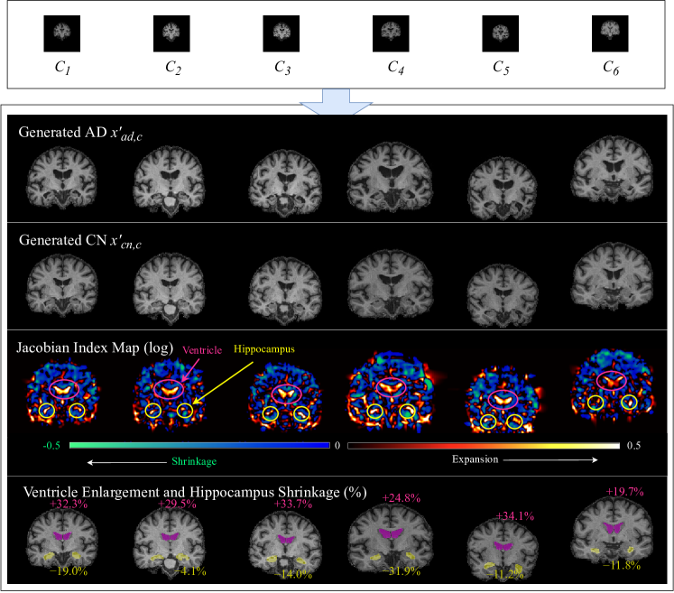
(a) Examples of generated AD $x^{\prime}_{ad,c}$, CN $x^{\prime}_{cn,c}$ coronal slices and Jacobian index maps in log scale. The Jacobian index values are associated with degrees of brain tissue expansion and shrinkage. Ventricular expansion and reduced hippocampal volume were estimated based on Jacobian index values of the manually drawn regions of interest (ROIs) (bottom sub-figure). Steps to acquire the Jacobian index maps and shrinkage estimates can be found in section S1.

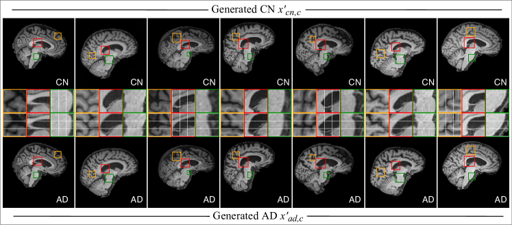
(b) Examples of generated AD $x^{\prime}_{ad,c}$, CN $x^{\prime}_{cn,c}$ sagittal slices also showing ventricular enlargement and cortical atrophy.

Figure 2: Example synthesised AD and CN pairs from DiDiGAN (more examples in Fig. S4). 2D Jacobian index was computed for the coronal view.

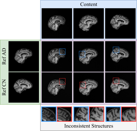
Fig. S1: StarGANv2 failed to retain structural consistency for meaningful comparative analysis.

Figure 2(a) shows examples of synthesised coronal AD ($x_{ad,c}^{\prime}$) and CN ($x_{cn,c}^{\prime}$) image pairs demonstrating high degrees of pair-wise structural similarities indicating good anatomical correspondence. AD-associated brain volume loss between each sample pair is quantified by the corresponding Jacobian index map [17] (registration-based morphometry). Consistent with the expected progression of AD[18][19], ventricular enlargement, reduced hippocampal volume and cortical atrophy are evident (high Jacobian index values indicating regional expansion in cerebrospinal fluid (CSF)). Figure 2(a) (bottom) shows manually drawn regions of interest for the ventricular and hippocampal areas. Across the 6 sample pairs, the Jacobian index values suggest an average ventricular area increase of 29.0% and an average hippocampal area reduction of 15.3% reduction. The coronal view results are further corroborated by an independent experiment performed on the sagittal view slices where reduced hippocampal volume and cortical atrophy are also visible through side-by-side comparison (Figure 2(b)). A StarGANv2 and a CycleGAN were also trained as baseline methods, but no usable results could be obtained for comparative analysis. StarGAN failed to establish anatomical correspondence, while CycleGAN failed to convey any difference between AD and CN, at all (Fig. S1 and S2).

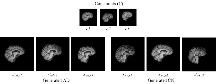
Fig. S3: Results without anti-aliasing. $x^{\prime}_{ad,c}$ and $x^{\prime}_{cn,c}$ were generated from structural constraints $c1,c2$ and $c3$. There are excessive non-AD variations which makes side-by-side comparison meaningless.

Anti-aliasing is especially important in DiDiGAN’s generator. The anti-aliasing issue raised in StyleGAN3 [12] translates to uncontrollable structural variations unrelated to the disease. Despite the use of a structural constrain $c$, the model is unable to maintain more fine-grained anatomical correspondence (especially in the cortical areas) due to aliasing. Example results synthesised without anti-aliasing can be found in Fig. S3

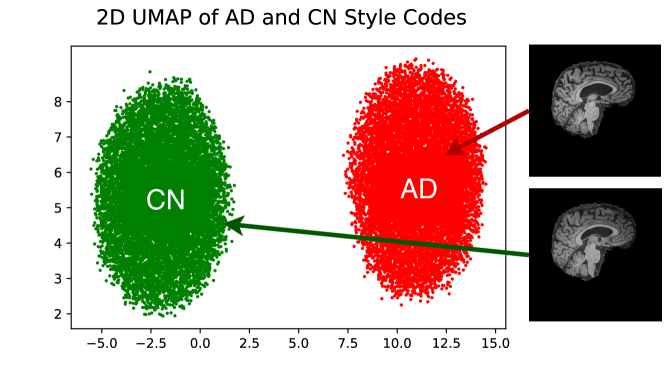
Figure 3: 2D UMAP visualisation of the 512-dimensional manifold. 10,000 style codes from each domain are sampled and the UMAP algorithm is configured to focus on global structures in the distribution.

Figure 3 shows a 2D UMAP [20] projection of AD and CN style codes sampled from the manifold (with different noise input). The two classes (disease / non-disease) form two distinctly separate clusters on the manifold. There is no overlap between the two distributions by design, which ensures AD features can be observed from any AD-CN pair regardless of the noise vectors used. It was also noted that traversing the manifold through different noise vectors within each disease / non-disease class introduces minor non-disease (such as contrast) variations.

Table I: 2D and 3D AD and CN classification results on the ADNI dataset.

Ref	Method	Test Accuracy	2D/3D
Valliani et al. [21]	ResNet-18	81.3%	2D
Wen et al. [22]	Pre-trained ImageNet + fine-tuning	79%	2D
Li et al. [23]	3D CNN	88%	3D
Senanayake et al [24]	3D CNN	76%	3D
Korolev et al [25]	3D CNN	80%	3D
Cheng et al [26]	3D CNN	87%	3D
DiDiGAN	Pre-trained $D$ without fine-tuning	82.3%	2D
DiDiGAN	Pre-trained $D$ + fine-tuning	86.5%	2D

A 2D U-Net [27] was used to estimate (slice by slice) the systematic brain volume loss exhibited in the generated coronal AD and CN pairs. The U-Net was trained for 3-class segmentation (grey matter, white matter and CSF) on the real data using labels generated from SPM [16]) (because no manual ones are available). Although these labels are not manual, the quality would suffice for estimating a general trend for two large groups of samples. The fake samples to be analysed were generated using down-sampled real test data as constraints and $y_{ad}$ and $y_{cn}$ as disease conditions. When running inference on the fake data slice by slice, the U-Net did not output extreme values (such as excessively different area estimates). This is an indication that the generated data distribution is similar to the real one as deep learning tend to fail catastrophically on unseen distributions. Between the synthesised AD and CN slices, the U-Net predicted average shrinkage values of 5.5%, 6.8% and 10.4% for the grey matter, white matter and CSF, respectively, which is in line with the trend found in the real data.

DiDiGAN’s ability to learn and synthesise AD features can be further verified through 2D AD-CN classification (on the ADNI dataset). It was noted that without any re-tuning, the $D_{w}$ head of a pre-trained discriminator already demonstrated good classification accuracy on the test set despite being limited to 2D. (Table I). With some re-tuning (1000 samples), the discriminator easily exceeds the test set accuracy of other 2D comparable methods, even approaching the accuracies of some 3D methods . Since the generator’s performance is tightly coupled with the discriminator, a good AD classification accuracy induces more confidence in the validity of the synthesised samples.

There are, however, some limitations of the current work. Since DiDiGAN is a weakly-supervised framework, evaluation is challenging due to the lack of labels specific to disease appearances. Indirect and manual methods, as shown in this work, are still required in the process. Nonetheless, DiDiGAN’s visualisation could still direct the focus of manual analysis to potential ROIs. As a GAN framework, there is some inherent instabilities during the training process, manual monitoring of convergence is required due to the lack of universal quality metrics for GANs in medical image analysis.

DiDiGAN presents a range of directions for future work. First, the manifold clusters should be further investigated for insights. It would also be valuable to encode additional clinical information such as age and gender onto the manifold to assess relationships between different data formats. Second, the structural constraint could incorporate human-decision making in the loop to direct the “attention" of DiDiGAN. For example, selectively down-sampling human-defined ROIs while leaving the rest of the constraint in full resolution could capture disease characteristics local to those ROIs. Finally, DiDiGAN showed promising results on the ADNI dataset. It would be valuable to test it on datasets collected for other diseases.

IV Conclusion

DiDiGAN demonstrated an excellent capacity to discover and aid disease characteristic visualisation from weakly-labelled medical images. Since many disease characteristics are extremely subtle,DiDiGAN learns a disease manifold to create a pair of AD and CN images with a shared anatomical structure. The major technical novelties of DiDiGAN are I) the use of a learnt disease manifold to influence the expression of AD features and II) mechanisms including the structural constraint and III) anti-aliasing to maintain anatomical correspondence. In the experiments involving the ADNI dataset, DiDiGAN discovered key AD features, including reduced hippocampal volume, ventricular enlargement and cortical atrophy. These results demonstrated DiDiGAN’s capability as a data-driven disease characteristic discovery method and future work will apply it to more dataset involving different diseases.

S1 Jacobian Index Computation

2-dimensional non-linear Symmetric Diffeomorphic Image Registration with Cross-Correlation (SyN-CC) (Avants et al. 2008) cost function as implemented in Advanced Normalization Tool (ANTS v.2.3.4 (Kim et al. 2008)) was conducted with the generated CN images being the fixed images and the generated AD images being the moving images. The $antsRegistration$ command was used for this image registration step. Jacobian Indices were calculated from the warp field obtained from the image registration step above using the $CreateJacobianDeterminantImage$. The Jacobian Index map was scaled and displayed as log Jacobian, so that the distribution is symmetrical around zero, with positive and negative values indicating volume expansion and contraction, respectively.

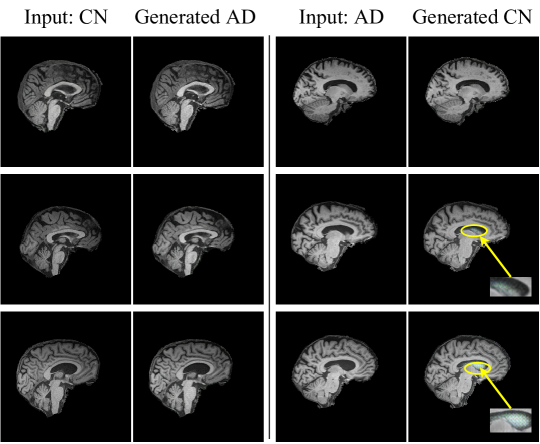
Fig. S2: CycleGAN created almost identical AD and CN images and some result contained artifacts.

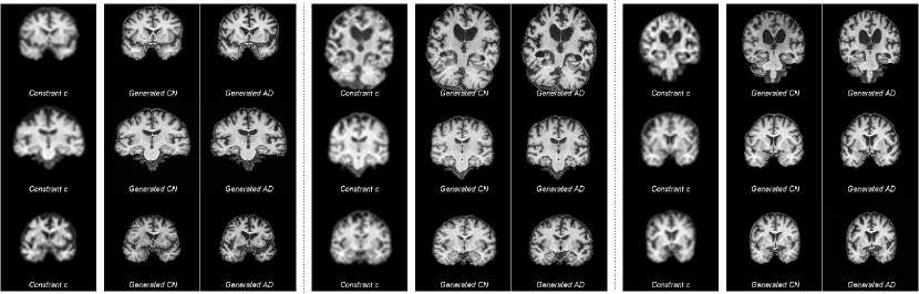
Fig. S4: Additional results based on more diverse brain structures (more extreme slice locations).

References

- [1] B. H. Menze, A. Jakab, S. Bauer, J. Kalpathy-Cramer, K. Farahani, J. Kirby, Y. Burren, N. Porz, J. Slotboom, R. Wiest, L. Lanczi, E. Gerstner, M.-A. Weber, T. Arbel, B. B. Avants, N. Ayache, P. Buendia, D. L. Collins, N. Cordier, J. J. Corso, A. Criminisi, T. Das, H. Delingette, C. Demiralp, C. R. Durst, M. Dojat, S. Doyle, J. Festa, F. Forbes, E. Geremia, B. Glocker, P. Golland, X. Guo, A. Hamamci, K. M. Iftekharuddin, R. Jena, N. M. John, E. Konukoglu, D. Lashkari, J. A. Mariz, R. Meier, S. Pereira, D. Precup, S. J. Price, T. R. Raviv, S. M. S. Reza, M. Ryan, D. Sarikaya, L. Schwartz, H.-C. Shin, J. Shotton, C. A. Silva, N. Sousa, N. K. Subbanna, G. Szekely, T. J. Taylor, O. M. Thomas, N. J. Tustison, G. Unal, F. Vasseur, M. Wintermark, D. H. Ye, L. Zhao, B. Zhao, D. Zikic, M. Prastawa, M. Reyes, and K. V. Leemput, “The multimodal brain tumor image segmentation benchmark (BRATS),” vol. 34, no. 10, pp. 1993–2024, Oct. 2015. [Online]. Available: https://doi.org/10.1109/tmi.2014.2377694
- [2] R. R. Selvaraju, M. Cogswell, A. Das, R. Vedantam, D. Parikh, and D. Batra, “Grad-CAM: Visual explanations from deep networks via gradient-based localization.” IEEE, Oct. 2017. [Online]. Available: https://doi.org/10.1109/iccv.2017.74
- [3] I. Goodfellow, J. Pouget-Abadie, M. Mirza, B. Xu, D. Warde-Farley, S. Ozair, A. Courville, and Y. Bengio, “Generative adversarial nets,” in Advances in Neural Information Processing Systems, Z. Ghahramani, M. Welling, C. Cortes, N. Lawrence, and K. Q. Weinberger, Eds., vol. 27. Curran Associates, Inc., 2014. [Online]. Available: https://proceedings.neurips.cc/paper/2014/file/5ca3e9b122f61f8f06494c97b1afccf3-Paper.pdf
- [4] T. Karras, S. Laine, and T. Aila, “A style-based generator architecture for generative adversarial networks,” in 2019 IEEE/CVF Conference on Computer Vision and Pattern Recognition (CVPR), 2019, pp. 4396–4405.
- [5] T. Karras, S. Laine, M. Aittala, J. Hellsten, J. Lehtinen, and T. Aila, “Analyzing and improving the image quality of stylegan,” in Proceedings of the IEEE/CVF Conference on Computer Vision and Pattern Recognition (CVPR), June 2020.
- [6] Z. Wu, D. Lischinski, and E. Shechtman, “Stylespace analysis: Disentangled controls for stylegan image generation,” in Proceedings of the IEEE/CVF Conference on Computer Vision and Pattern Recognition, 2021, pp. 12 863–12 872.
- [7] O. Patashnik, Z. Wu, E. Shechtman, D. Cohen-Or, and D. Lischinski, “Styleclip: Text-driven manipulation of stylegan imagery,” in Proceedings of the IEEE/CVF International Conference on Computer Vision, 2021, pp. 2085–2094.
- [8] Y. Choi, M. Choi, M. Kim, J.-W. Ha, S. Kim, and J. Choo, “StarGAN: Unified generative adversarial networks for multi-domain image-to-image translation.” IEEE, Jun. 2018. [Online]. Available: https://doi.org/10.1109/cvpr.2018.00916
- [9] Y. Choi, Y. Uh, J. Yoo, and J.-W. Ha, “StarGAN v2: Diverse image synthesis for multiple domains.” IEEE, Jun. 2020. [Online]. Available: https://doi.org/10.1109/cvpr42600.2020.00821
- [10] A. Chartsias, T. Joyce, G. Papanastasiou, S. Semple, M. Williams, D. E. Newby, R. Dharmakumar, and S. A. Tsaftaris, “Disentangled representation learning in cardiac image analysis,” Medical Image Analysis, vol. 58, p. 101535, Dec. 2019. [Online]. Available: https://doi.org/10.1016/j.media.2019.101535
- [11] R. Zhang, “Making convolutional networks shift-invariant again,” in ICML, 2019.
- [12] T. Karras, M. Aittala, S. Laine, E. Härkönen, J. Hellsten, J. Lehtinen, and T. Aila, “Alias-free generative adversarial networks,” in Proc. NeurIPS, 2021.
- [13] C. Shannon, “Communication in the presence of noise,” Proceedings of the IRE, vol. 37, no. 1, pp. 10–21, jan 1949. [Online]. Available: https://doi.org/10.1109/jrproc.1949.232969
- [14] L. M. Mescheder, A. Geiger, and S. Nowozin, “Which training methods for gans do actually converge?” in ICML, 2018.
- [15] N. J. Tustison, B. B. Avants, P. A. Cook, Y. Zheng, A. Egan, P. A. Yushkevich, and J. C. Gee, “N4itk: Improved n3 bias correction,” vol. 29, no. 6, pp. 1310–1320, Jun. 2010. [Online]. Available: https://doi.org/10.1109/tmi.2010.2046908
- [16] N. Tzourio-Mazoyer, B. Landeau, D. Papathanassiou, F. Crivello, O. Etard, N. Delcroix, B. Mazoyer, and M. Joliot, “Automated anatomical labeling of activations in spm using a macroscopic anatomical parcellation of the mni mri single-subject brain,” Neuroimage, vol. 15, no. 1, pp. 273–289, 2002.
- [17] B. B. Avants, N. J. Tustison, G. Song, P. A. Cook, A. Klein, and J. C. Gee, “A reproducible evaluation of ANTs similarity metric performance in brain image registration,” NeuroImage, vol. 54, no. 3, pp. 2033–2044, Feb. 2011. [Online]. Available: https://doi.org/10.1016/j.neuroimage.2010.09.025
- [18] N. Schuff, N. Woerner, L. Boreta, T. Kornfield, L. Shaw, J. Trojanowski, P. Thompson, C. Jack Jr, M. Weiner, and A. D. N. Initiative, “Mri of hippocampal volume loss in early alzheimer’s disease in relation to apoe genotype and biomarkers,” Brain, vol. 132, no. 4, pp. 1067–1077, 2009.
- [19] M. R. Sabuncu, R. S. Desikan, J. Sepulcre, B. T. T. Yeo, H. Liu, N. J. Schmansky, M. Reuter, M. W. Weiner, R. L. Buckner, R. A. Sperling et al., “The dynamics of cortical and hippocampal atrophy in alzheimer disease,” Archives of neurology, vol. 68, no. 8, pp. 1040–1048, 2011.
- [20] L. McInnes, J. Healy, N. Saul, and L. Grossberger, “Umap: Uniform manifold approximation and projection,” The Journal of Open Source Software, vol. 3, no. 29, p. 861, 2018.
- [21] A. Valliani and A. Soni, “Deep residual nets for improved alzheimer’s diagnosis,” in Proceedings of the 8th ACM International Conference on Bioinformatics, Computational Biology, and Health Informatics, 2017, pp. 615–615.
- [22] J. Wen, E. Thibeau-Sutre, M. Diaz-Melo, J. Samper-González, A. Routier, S. Bottani, D. Dormont, S. Durrleman, N. Burgos, O. Colliot et al., “Convolutional neural networks for classification of alzheimer’s disease: Overview and reproducible evaluation,” Medical image analysis, vol. 63, p. 101694, 2020.
- [23] F. Li, D. Cheng, and M. Liu, “Alzheimer’s disease classification based on combination of multi-model convolutional networks,” in 2017 IEEE international conference on imaging systems and techniques (IST). IEEE, 2017, pp. 1–5.
- [24] U. Senanayake, A. Sowmya, and L. Dawes, “Deep fusion pipeline for mild cognitive impairment diagnosis,” in 2018 IEEE 15th international symposium on biomedical imaging (isbi 2018). IEEE, 2018, pp. 1394–1997.
- [25] S. Korolev, A. Safiullin, M. Belyaev, and Y. Dodonova, “Residual and plain convolutional neural networks for 3d brain mri classification,” in 2017 IEEE 14th international symposium on biomedical imaging (ISBI 2017). IEEE, 2017, pp. 835–838.
- [26] D. Cheng, M. Liu, J. Fu, and Y. Wang, “Classification of mr brain images by combination of multi-cnns for ad diagnosis,” in Ninth international conference on digital image processing (ICDIP 2017), vol. 10420. SPIE, 2017, pp. 875–879.
- [27] O. Ronneberger, P. Fischer, and T. Brox, “U-net: Convolutional networks for biomedical image segmentation,” in Medical Image Computing and Computer-Assisted Intervention – MICCAI 2015, N. Navab, J. Hornegger, W. M. Wells, and A. F. Frangi, Eds. Cham: Springer International Publishing, 2015, pp. 234–241.