Over-the-Air Computation over Balanced Numerals

Abstract

In this study, a digital over-the-air computation (OAC) scheme for achieving continuous-valued gradient aggregation is proposed. It is shown that the average of a set of real-valued parameters can be calculated approximately by using the average of the corresponding numerals, where the numerals are obtained based on a balanced number system. By using this property, the proposed scheme encodes the local gradients into a set of numerals. It then determines the positions of the activated orthogonal frequency division multiplexing (OFDM) subcarriers by using the values of the numerals. To eliminate the need for a precise sample-level time synchronization, channel estimation overhead, and power instabilities due to the channel inversion, the proposed scheme also uses a non-coherent receiver at the edge server (ES) and does not utilize a pre-equalization at the edge devices. Finally, the theoretical MSE performance of the proposed scheme is derived and its performance for federated edge learning (FEEL) is demonstrated.

I Introduction

OAC aims to compute nomographic functions by exploiting the signal-superposition property of wireless multiple-access channels [1, 2]. OAC, which initially considered for wireless sensor networks [3], has recently gained increasing attention for applications such as distributed learning or wireless control systems [4, 5, 6]. For example, FEEL, one of the promising distributed edge learning frameworks, aims to implement federated learning (FL) [7] over a wireless network. With FEEL, the task of model training is distributed across multiple EDs and the data uploading is avoided to promote user-privacy [8, 5]. Instead of data samples, EDs share a large number of local stochastic gradients (or local model parameters) with an ES for aggregation, e.g., averaging. However, typical orthogonal user multiplexing methods such as orthogonal frequency division multiple access (OFDMA) can be wasteful in this scenario since the ES may not be interested in the local information of the EDs but only in a function of them.

Although OAC is a promising concept to address the latency issues for FEEL, it is challenging to realize a reliable OAC scheme due to the detrimental impact of wireless channels on the OAC. To address this issue, a majority of the state-of-the-art OAC methods relying on pre-equalization techniques[9, 10, 11, 12, 13]. However, a pre-equalizer can impose stringent requirements on the underlying mechanisms such as time-frequency synchronization, channel estimation, and channel prediction, which can be challenging to satisfy under the non-stationary channel conditions [14]. Another issue is that most of the OAC schemes use analog modulation schemes to achieve a continuous-valued computation. However, analog modulations are more susceptible to noise as compared to digital schemes. Although there are digital aggregation methods, e.g., one-bit broadband digital aggregation (OBDA) [12], -based (FSK-MV) [15], and -based (PPM-MV) [16], by relying on specific training approaches, i.e., distributed training by the MV with sign stochastic gradient descent (signSGD) [17], these schemes do not allow one to compute a continuous-valued function.

In this paper, to address the aforementioned issues, we introduce an OAC scheme for FEEL, where the local gradients are encoded into a set of numerals based on a balanced number system (also called balanced numeral system or signed-digit representation) [18] to achieve a continuous-valued computation over a digital scheme. The proposed method does not rely on pre-equalization and the availability of channel state information (CSI) at the EDs and the ES, which relaxes the synchronization requirements at the EDs and the ES. We demonstrate the efficacy of the proposed OAC scheme for both homogeneous and heterogeneous data distribution scenarios.

Notation: The sets of complex numbers, real numbers, integers, and integers modulo $H$ are denoted by $\mathbb{C}$, $\mathbb{R}$, $\mathbb{Z}$, and $\mathbb{Z}_{H}$ respectively. The $N$-dimensional all zero vector and the $N\times N$ identity matrix are $\textbf{{0}}_{N}$ and ${\textbf{{I}}_{N}}$, respectively. The function $\mathbb{I}\left[{\cdot}\right]$ results in $1$ if its argument holds, otherwise it is $0$. ${\mathbb{E}}\left[\cdot\right]$ is the expectation of its argument. $\nabla f(\textbf{w})$ denotes the gradient of the function $f$, i.e. $\nabla f$, at the point w. The zero-mean circularly symmetric multivariate complex Gaussian distribution with the covariance matrix ${\textbf{{C}}_{M}}$ of an $M$-dimensional random vector $\textbf{{x}}\in\mathbb{C}^{M\times 1}$ is denoted by $\textbf{{x}}\sim\mathcal{CN}({\textbf{{0}}_{M},\textbf{{C}}_{M}})$. The gamma distribution with the shape parameter $n$ and the rate $\lambda$ is $\Gamma({n,\lambda})$. The $\ell_{2}$-norm of the vector x is $\lVert\textbf{{x}}\rVert_{2}$.

II System Model

We consider a network with $K$ EDs that are connected to an ES wirelessly, where each ED and the ES are equipped with a single antenna and $R$ antennas, respectively. We assume that the large-scale impact of the wireless channel is compensated with a power control mechanism to maintain the average received signal power of each ED at the ES identical. For the signal model, we assume that the EDs access the wireless channel on the same time-frequency resources simultaneously with $S$ OFDM symbols consisting of $M$ active subcarriers for OAC. Assuming that the cyclic prefix (CP) duration is larger than the sum of maximum time-synchronization error and maximum-excess delay of the channel, we express the received symbol on the $l$th subcarrier of the $m$th OFDM symbol at the ES for the $\mathscr{t}$th communication round of the training as

$$\textbf{r}_{l,m}^{(\mathscr{t})}=\sum_{k=0}^{K-1}\textbf{h}_{k,l,m}^{(\mathscr{t})}t_{k,l,m}^{(\mathscr{t})}+\textbf{n}_{l,m}^{(\mathscr{t})}~{},$$ (1)

where $\textbf{h}_{k,l,m}^{(\mathscr{t})}\sim\mathcal{CN}({\textbf{{0}}_{R},{\textbf{{I}}_{R}}})$ is a vector that consists of the channel coefficients between $R$ antennas at the ES and the $k$th ED, $t_{k,l,m}^{(\mathscr{t})}\in\mathbb{C}$ is the transmitted modulation symbol from the $k$th ED, and ${\textbf{n}_{l,m}^{(\mathscr{t})}}\sim\mathcal{CN}({\textbf{{0}}_{R},\sigma_{\rm n}^{2}{\textbf{{I}}_{R}}})$ is the additive white Gaussian noise (AWGN), where $\sigma_{\rm n}^{2}$ is the noise variance for $l\in\mathbb{Z}_{M}$ and $m\in\mathbb{Z}_{S}$. We denote the signal-to-noise ratio (SNR) of an ED at the ES receiver as $1/\sigma_{\rm n}^{2}$.

In practice, the synchronization point where the discrete Fourier transform (DFT) starts to be applied to the received signal for demodulation at the ES and the time synchronization across the EDs may not be precise. To model former impairment, we assume that synchronization point can deviate by $N_{\text{err}}$ samples within the CP window. For the latter impairment, the time of arrivals of the EDs’ signals at the ES location are sampled from a uniform distribution between $0$ and $T_{\rm sync}$ seconds, where $T_{\rm sync}$ is equal to the reciprocal to the signal bandwidth. Note the coarse time-synchronization can be maintained with the state-of-the-art protocols used in cellular systems. We introduce additional phase rotations to $\textbf{h}_{k,l,m}^{(\mathscr{t})}$ to capture the impact of the time-synchronization errors on $\textbf{r}_{l,m}^{(\mathscr{t})}$.

II-A Balanced Number Systems

Let $f_{\text{enc},\beta}$ be a function that maps $v\in\mathbb{R}$ to a sequence of $D$ elements (i.e., numerals) in $\{\left(x_{D-1},\hbox to10.00002pt{.\hss.\hss.},x_{1},x_{0}\right)|x_{i}\in\mathbb{S}_{\beta},\beta>1,i\in\mathbb{Z}_{D}\}$ as

$$\left(x_{D-1},\hbox to10.00002pt{.\hss.\hss.},x_{1},x_{0}\right)=f_{\text{enc},\beta}(v)~{},$$ (2)

where $\beta$ is the base (also called scale [19]), $x_{i}$ is referred to as a numeral at the $i$th position, and $\mathbb{S}_{\beta}$ is the symbol set with base $\beta$. In this study, we consider a balanced number system for expressing $f_{\text{enc},\beta}$ and assume that $\beta$ is an odd positive integer. The numerals are obtained as follows: For a given $v$ for $|v|\leq v_{\rm max}$, the encoder $f_{\text{enc},\beta}(v)$ first computes the base-$\beta$ representation of the rounded, biased, and normalized $v$ as

$$\left\lfloor\frac{\xi}{v_{\rm max}}v+\xi+\frac{1}{2}\right\rfloor\triangleq\sum_{i=0}^{D-1}b_{i}\beta^{i}~{},$$ (3)

for $\xi\triangleq{(\beta^{D}-1)}/{2}$ and $b_{i}\in\mathbb{Z}_{\beta}$. Afterwards, it calculates $x_{i}$ as $x_{i}\triangleq b_{i}-(\beta-1)/2$, $\forall i\in\mathbb{Z}_{D}$. Hence, $\mathbb{S}_{\beta}$ can be defined as

$$\mathbb{S}_{\beta}\triangleq\{a_{j}|a_{j}=f_{\rm bal}(j),j\in\mathbb{Z}_{\beta}\}~{},$$ (4)

where $f_{\rm bal}(j)$ is given by

$$f_{\rm bal}(j)\triangleq\begin{cases}-(j+1)/2,&\text{odd }j,j<\beta-1\\ (j+2)/2,&\text{even }j,j<\beta-1\\ 0,&j=\beta-1\end{cases}~{}.$$ (5)

Based on (5), $a_{\beta-1}$ is a zero-valued symbol. The example symbol sets for $\beta=5$ and $\beta=7$ can obtained as $\mathbb{S}_{5}=\{-1,1,-2,2,0\}$ and $\mathbb{S}_{7}=\{-1,1,-2,2,-3,3,0\}$ , respectively. For a balanced number system, there is no dedicated symbol for the sign of $v$ as $\mathbb{S}_{\beta}$ contains negative-valued symbols.

Example 1.

Assume that $\beta=5$, $D=3$, and $v_{\rm max}=1$ and we want to calculate $f_{\text{enc},\beta}(0.28)$ and $f_{\text{enc},\beta}(-0.86)$. By the definition, $\xi=(5^{2}-1)/2=62$. The base 5 representations of the decimal $\lfloor 62\times 0.28+62+1/2\rfloor=79$ and the decimal $\lfloor 62\times-0.86+62+1/2\rfloor=9$ are $({b_{2}b_{1}b_{0}})_{5}=(304)_{5}$ and $({b_{2}b_{1}b_{0}})_{5}=(014)_{5}$, respectively. Since $x_{i}\triangleq b_{i}-(\beta-1)/2$, we obtain $f_{\text{enc},\beta}(0.28)=\left(1,-2,2\right)$, and $f_{\text{enc},\beta}(-0.86)=\left(-2,-1,2\right)$.

The corresponding decoder $f_{\text{dec},\beta}$ that maps the sequence $\left(x_{D-1},\hbox to10.00002pt{.\hss.\hss.},x_{1},x_{0}\right)$ to $\bar{v}\in\mathbb{R}$ can be expressed as

$$\bar{v}=f_{\text{dec},\beta}\left(x_{D-1},\hbox to10.00002pt{.\hss.\hss.},x_{1},x_{0}\right)\triangleq\frac{v_{\rm max}}{\xi}\sum_{i=0}^{D-1}x_{i}\beta^{i}~{}.$$ (6)

Note that $\bar{v}=f_{\text{dec},\beta}f_{\text{enc},\beta}(v)$ forms a mid-tread uniform quantization, i.e., zero is one of the re-construction levels. The quantization step size can also be calculated as $\Delta=2v_{\rm max}/(\beta^{D}-1)$ and the quantization error, i.e., $|{v-\bar{v}}|$, decreases with increasing $D$ for $|v|\leq v_{\rm max}$.

Example 2.

Consider the parameters given in Example 1. Hence, we obtain $f_{\text{dec},\beta}f_{\text{enc},\beta}(0.28)=f_{\text{dec},\beta}\left(1,-2,2\right)\approxeq 0.2742$, and $f_{\text{dec},\beta}f_{\text{enc},\beta}(-0.86)=f_{\text{dec},\beta}\left(-2,-1,2\right)\approxeq-0.8548$ based on (6). The step size can also be calculated as $\Delta=2/(5^{3}-1)\approxeq 0.016$.

II-B Learning Model

Let $\mathcal{D}_{k}$ denote the local data set containing the labeled data samples $({\textrm{{x}}}_{{\ell}},{y}_{{\ell}})$ at the $k$th ED, $\forall k\in\mathbb{Z}_{K}$, where ${\textrm{{x}}}_{{\ell}}$ is the ${\ell}$th data sample with its ground truth label ${y}_{{\ell}}$. Suppose that all EDs upload their data sets to the ES. The centralized learning problem can then be expressed as

$${\textbf{w}^{*}}=\arg\min_{\textbf{w}\in\mathbb{R}^{Q}}F(\textbf{w})=\arg\min_{\textbf{w}\in\mathbb{R}^{Q}}\frac{1}{|\mathcal{D}|}\sum_{\forall({\textrm{{x}}}_{{\ell}},{y}_{{\ell}})\in\mathcal{D}}f(\textbf{w};{\textrm{{x}}}_{{\ell}},{y}_{{\ell}})~{},$$

where $F(\textbf{w})$ is the loss function, $\mathcal{D}=\mathcal{D}_{0}\cup\mathcal{D}_{1}\cup\cdots\cup\mathcal{D}_{K-1}$ is complete data set, and $f(\textbf{w};{\textrm{{x}}}_{{\ell}},{y}_{{\ell}})$ is the sample loss function for the parameters $\textbf{w}=[{w}_{0},\hbox to10.00002pt{.\hss.\hss.},{w}_{Q-1}]^{\rm T}\in\mathbb{R}^{Q}$, and $Q$ is the number of parameters. With (full-batch) gradient descent, a local optimum point can be obtained as

$$\textbf{w}^{(\mathscr{t}+1)}=\textbf{w}^{(\mathscr{t})}-\eta{\textbf{{g}}}^{(\mathscr{t})}~{},$$ (7)

where $\eta$ is the learning rate and the gradient vector ${\textbf{{g}}}^{(\mathscr{t})}=[{{g}}^{(\mathscr{t})}_{0},\hbox to10.00002pt{.\hss.\hss.},{{g}}^{(\mathscr{t})}_{Q-1}]^{\rm T}\in\mathbb{R}^{Q}$ can be expressed as

$${\textbf{{g}}}^{(\mathscr{t})}=\nabla F(\textbf{w}^{(\mathscr{t})})=\frac{1}{|\mathcal{D}|}\sum_{\forall({\textrm{{x}}}_{{\ell}},{y}_{{\ell}})\in\mathcal{D}}\nabla f(\textbf{w}^{(\mathscr{t})};{\textrm{{x}}}_{{\ell}},{y}_{{\ell}})~{}.$$ (8)

The equation (7) can be re-written as

$$\textbf{w}^{(\mathscr{t}+1)} =\textbf{w}^{(\mathscr{t})}-\eta\sum_{k=0}^{K-1}{\frac{|\mathcal{D}_{k}|}{|\mathcal{D}|}}\underbrace{\frac{1}{|\mathcal{D}_{k}|}\sum_{\forall({\textrm{{x}}}_{{\ell}},{y}_{{\ell}})\in\mathcal{D}_{k}}\nabla f(\textbf{w}^{(\mathscr{t})};{\textrm{{x}}}_{{\ell}},{y}_{{\ell}})}_{\triangleq{\textbf{g}}_{k}^{(\mathscr{t})}}~{},$$

where ${\textbf{g}}_{k}^{(\mathscr{t})}\in\mathbb{R}^{Q}$ denotes the local gradient vector at the $k$th ED. Therefore, (7) can still be realized by communicating the local gradients or locally updated model parameters between the EDs and the ES, rather than moving the local data sets from the EDs to the ES, which is beneficial for promoting data privacy [8, 5]. It also shows the underlying principle of the plain FL based on gradient or parameter aggregations [7].

FEEL aims to realize FL over a wireless network. In this study, we consider FL based on SGD, known as FedSGD [7], over a wireless network: The $k$th ED calculates an estimate of the local gradients, denoted by $\tilde{\textbf{g}}_{k}^{(\mathscr{t})}=[{\tilde{g}}_{k,0}^{(\mathscr{t})},\hbox to10.00002pt{.\hss.\hss.},{\tilde{g}}_{k,Q-1}^{(\mathscr{t})}]^{\rm T}\in\mathbb{R}^{Q}$, as

$$\tilde{\textbf{g}}_{k}^{(\mathscr{t})}=\nabla F_{k}(\textbf{w}^{(\mathscr{t})})=\frac{1}{n_{\rm b}}\sum_{\forall({\textrm{{x}}}_{{\ell}},{y}_{{\ell}})\in\mathcal{\tilde{D}}_{k}}\nabla f(\textbf{w}^{(\mathscr{t})};{\textrm{{x}}}_{{\ell}},{y}_{{\ell}})~{},$$ (9)

where $\mathcal{\tilde{D}}_{k}\subset\mathcal{D}_{k}$ is the data batch obtained from the local data set and $n_{\rm b}=|\mathcal{\tilde{D}}_{k}|$ as the batch size. The EDs transmit the local gradient estimates to the ES. Assuming identical data set sizes across the EDs, the ES calculates the average stochastic gradient vector $\textbf{v}^{(\mathscr{t})}\triangleq[{v}^{(\mathscr{t})}_{0},\hbox to10.00002pt{.\hss.\hss.},{v}^{(\mathscr{t})}_{Q-1}]^{\rm T}=\frac{1}{K}\sum_{k=0}^{K-1}\tilde{\textbf{g}}_{k}^{(\mathscr{t})}$ and broadcasts it to the EDs. Finally, the model parameters at the EDs are updated as $\textbf{w}^{(\mathscr{t}+1)}=\textbf{w}^{(\mathscr{t})}-\eta\textbf{v}^{(\mathscr{t})}$.

With a traditional orthogonal user multiplexing, the per-round communication latency for FEEL linearly increases with the number of EDs [20]. With the motivation of eliminating per-round communication latency, the main objective of this work is to calculate an estimate of $\textbf{v}^{(\mathscr{t})}$, denoted by $\hat{\textbf{{v}}}^{(\mathscr{t})}\triangleq[{\hat{v}}^{(\mathscr{t})}_{0},\hbox to10.00002pt{.\hss.\hss.},{\hat{v}}^{(\mathscr{t})}_{Q-1}]^{\rm T}$, through a digital OAC scheme robust against fading channel.

III Proposed OAC Scheme

Based on the discussions given in Section II-B, consider the $q$th gradient at the $k$th ED for the $\mathscr{t}$th communication round of the FEEL, i.e., ${\tilde{g}}_{k,q}^{(\mathscr{t})}$. For a given $\beta$, suppose that ${\tilde{g}}_{k,q}^{(\mathscr{t})}$ is encoded into the sequence of length $D$ denoted by

$$\left(d_{{k,q},{D-1}}^{(\mathscr{t})},\hbox to10.00002pt{.\hss.\hss.},d_{{k,q},{1}}^{(\mathscr{t})},d_{{k,q},{0}}^{(\mathscr{t})}\right)=f_{\text{enc},\beta}({\tilde{g}}_{k,q}^{(\mathscr{t})})~{},$$ (10)

for $d_{{k,q},{i}}^{(\mathscr{t})}\in\mathbb{S}_{\beta}$. By using definition of $f_{\text{dec},\beta}$ in (6), the $q$th average stochastic gradient, i.e., ${v}^{(\mathscr{t})}_{q}=\frac{1}{K}\sum_{k=0}^{K-1}{\tilde{g}}_{k,q}^{(\mathscr{t})}$, can be obtained approximately as

$${v}^{(\mathscr{t})}_{q}\approxeq{\bar{v}}^{(\mathscr{t})}_{q}\triangleq\frac{1}{K}\sum_{k=0}^{K-1} {\bar{\tilde{g}}}_{k,q}^{(\mathscr{t})}=\frac{v_{\rm max}}{\xi}\sum_{i=0}^{D-1}\underbrace{\frac{1}{K}\sum_{k=0}^{K-1}d_{{k,q},{i}}^{(\mathscr{t})}}_{\triangleq\mu_{{q},{i}}^{(\mathscr{t})}}\beta^{i}$$

$$=f_{\text{dec},\beta}\left(\mu_{{q},{D-1}}^{(\mathscr{t})},\hbox to10.00002pt{.\hss.\hss.},\mu_{{q},{1}}^{(\mathscr{t})},\mu_{{q},{0}}^{(\mathscr{t})}\right)~{},$$ (11)

where ${\bar{\tilde{g}}}_{k,q}^{(\mathscr{t})}$ is the quantized gradient, i.e., ${\bar{\tilde{g}}}_{k,q}^{(\mathscr{t})}=f_{\text{dec},\beta}f_{\text{enc},\beta}({\tilde{g}}_{k,q}^{(\mathscr{t})})$. Equation (11) implies that ${v}^{(\mathscr{t})}_{q}$ can be calculated approximately by evaluating the function $f_{\text{dec},\beta}$ with the values that are calculated by averaging the numerals across $K$ EDs in real domain, i.e., $\{\mu_{{q},{i}}^{(\mathscr{t})}|i\in\mathbb{Z}_{D}\}$. By evaluating $\mu_{{q},{i}}^{(\mathscr{t})}$ further, it can also be shown that

$$\mu_{{q},{i}}^{(\mathscr{t})}=\frac{1}{K}\sum_{k=0}^{K-1}d_{{k,q},{i}}^{(\mathscr{t})}=\frac{1}{K}\sum_{j=0}^{\beta-1}a_{j}U_{q,i,j}~{},$$ (12)

where $U_{q,i,j}$ denotes the number of EDs with the symbol $a_{j}$ for the $i$th numeral in (10) and the $q$th gradient. Note that the identity in (12) is due to the definition of expectation for discrete outcomes as given for a probability mass function.

Example 3.

Assume that $K=2$, ${\tilde{g}}_{0,q}^{(\mathscr{t})}=0.28$, and ${\tilde{g}}_{1,q}^{(\mathscr{t})}=-0.86$. The average of the gradients can be calculated as ${v}^{(\mathscr{t})}_{q}=({\tilde{g}}_{0,q}^{(\mathscr{t})}+{\tilde{g}}_{1,q}^{(\mathscr{t})})/2=-0.29$. Now, consider the encoder parameters given in Example 1. We obtain $f_{\text{enc},\beta}(0.28)=\left(1,-2,2\right)$, and $f_{\text{enc},\beta}(-0.86)=\left(-2,-1,2\right)$. Therefore, the average of the numerals can be calculated as $(\mu_{{q},{2}}^{(\mathscr{t})},\mu_{{q},{1}}^{(\mathscr{t})},\mu_{{q},{0}}^{(\mathscr{t})})=(1-2,-2-1,2+2)/2=(-1/2,-3/2,2)$. Also, notice that $(\mu_{{q},{2}}^{(\mathscr{t})},\mu_{{q},{1}}^{(\mathscr{t})},\mu_{{q},{0}}^{(\mathscr{t})})$ can be calculated by using the number of EDs that votes for each element of $\{-1,1,-2,2,0\}$. For instance, $\mu_{{q},{0}}^{(\mathscr{t})}$ can be calculated via the last expression in (12) for $(U_{q,i,0},U_{q,i,1},U_{q,i,2},U_{q,i,3},U_{q,i,4})=(0,0,0,2,0)$ where the corresponding symbols are $(a_{0},a_{1},a_{2},a_{3},a_{4})=(-1,1,-2,2,0)$ for $\beta=5$. Finally, by evaluating ${\bar{v}}^{(\mathscr{t})}_{q}=f_{\text{dec},\beta}(-1/2,-3/2,2)$, we obtain ${\bar{v}}^{(\mathscr{t})}_{q}\approxeq-0.2903$. Note that ${\bar{v}}^{(\mathscr{t})}_{q}$ is also equal to the average of the quantized gradients, i.e., $f_{\text{dec},\beta}f_{\text{enc},\beta}(0.28)\approxeq 0.2742$ and $f_{\text{dec},\beta}f_{\text{enc},\beta}(-0.86)\approxeq-0.8548$, as provided in Example 2.

The main equations used in this work are the encoding in (10), the expansion in (11), and the identity in (12), which enable one to calculate an estimate of ${v}^{(\mathscr{t})}_{q}$ by averaging numerals, rather than the actual values of the gradients.

III-A Edge Device - Transmitter

At the $\mathscr{t}$th communication round of the FEEL, the $k$th ED calculates the numerals $\{d_{{k,q},{i}}^{(\mathscr{t})}|q\in\mathbb{Z}_{Q},i\in\mathbb{Z}_{D}\}$ with (10), for a given $\beta$. The key strategy exploited at the $k$th ED with the proposed scheme is that $\beta-1$ subcarriers are dedicated for each numeral and one of these subcarriers is activated based on its value. To express this encoding operation rigorously, let $\mathcal{M}$ be a function that maps $q\in\mathbb{Z}_{Q}$ to a set of $(\beta-1)D$ distinct time-frequency index pairs denoted by $\mathbb{T}_{q}\triangleq\{(m_{i,\ell},l_{i,\ell})|i\in\mathbb{Z}_{D},\ell\in\mathbb{Z}_{\beta-1}\}$ for $m_{i,\ell}\in\mathbb{Z}_{S}$ and $l_{i,\ell}\in\mathbb{Z}_{M}$, where $\mathbb{T}_{q_{1}}\cap\mathbb{T}_{q_{2}}=\emptyset$ if $q_{1}\neq q_{2}$ for $q_{1},q_{2}\in\mathbb{Z}_{Q}$. The $k$th ED determines the modulation symbol $t_{k,{m_{i,\ell},l_{i,\ell}}}^{(\mathscr{t})}$ as

$$t_{k,{m_{i,\ell},l_{i,\ell}}}^{(\mathscr{t})}=\sqrt{E_{\rm s}}s_{k,q,i}^{(\mathscr{t})}\times\mathbb{I}\left[{d_{{k,q},{i}}^{(\mathscr{t})}=a_{\ell}}\right]~{},$$ (13)

for all $i\in\mathbb{Z}_{D}$ and $\ell\in\mathbb{Z}_{\beta-1}$, where $E_{\rm s}=\beta-1$ is a factor to normalize the OFDM symbol energy and $s_{k,q,i}^{(\mathscr{t})}$ is a randomization symbol on the unit circle for peak-to-mean envelope power ratio (PMEPR) reduction [15]. Note that we do not allocate a subcarrier for $a_{\beta-1}=0$ since it does not contribute to the sum given in (12). After the calculation of (13) for all gradients, the $k$th ED calculates the OFDM symbols and all EDs transmit them simultaneously based on the discussions in Section II. Since the proposed scheme uses $(\beta-1)D$ subcarriers for each gradient, the maximum number of gradients that can be transmitted on each OFDM symbol can be calculated as $M_{\rm par}=\lfloor M/((\beta-1)D)\rfloor$ for all EDs.

It is worth emphasizing that we do not use truncated-channel inversion (TCI) to compensate the impact of multipath channel on the transmitted symbols as this is beneficial to eliminate 1) the need for precise time synchronization, 2) the channel estimation overhead in a mobile wireless networks, 3) the information loss due to the truncation, and 4) the power instabilities in fading channel due to the channel inversion.

III-B Edge Server - Receiver

At the ES, we assume that the CSI, i.e., $\{\textbf{h}_{k,l,m}^{(\mathscr{t})}|k\in\mathbb{Z}_{K},l\in\mathbb{Z}_{M},m\in\mathbb{Z}_{S}\}$, is not available. Hence, the ES exploits that $\textbf{r}_{m_{i,\ell},l_{i,\ell}}^{(\mathscr{t})}$ is a random vector for $\textbf{r}_{m_{i,\ell},l_{i,\ell}}^{(\mathscr{t})}\sim\mathcal{CN}({\textbf{{0}}_{R},{(E_{\rm s}U_{q,i,\ell}+\sigma_{\rm n}^{2})}{{\textbf{{I}}_{R}}}})$ and obtains an estimate of $\{U_{q,i,\ell}|\ell\in\mathbb{Z}_{\beta-1}\}$ to realize the last expression in (12), non-coherently. For given $i$ and $q$, by using the corresponding log-likelihood function, the maximum likelihood (ML) detector can be expressed as

$$\{\hat{U}_{q,i,\ell}|\ell\in\mathbb{Z}_{\beta-1}\}=\arg\min_{\{{U}_{\forall\ell}\}}\left\{\sum_{\ell=0}^{\beta-2}\ln\det{\bf\Sigma}_{\ell}+{\rm\textbf{x}}_{\ell}^{\rm H}{\bf\Sigma}_{\ell}^{-1}{\rm\textbf{x}}_{\ell}\right\}$$ (14)

$$~{}~{}~{}~{}~{}~{}~{}~{}~{}~{}~{}~{}\text{s.t.}~{}{U}_{\ell}\in\{0,\hbox to10.00002pt{.\hss.\hss.},K\},\ell\in\mathbb{Z}_{\beta-1}~{},\sum_{\ell=0}^{\beta-2}{U}_{\ell}\leq K~{},$$

where ${\rm\textbf{x}}_{\ell}=[\Re\{\textbf{r}_{m_{i,\ell},l_{i,\ell}}^{(\mathscr{t})}\}^{\rm T}~{}\Im\{\textbf{r}_{m_{i,\ell},l_{i,\ell}}^{(\mathscr{t})}\}^{\rm T}]^{\rm T}$ and ${\bf\Sigma}_{\ell}=\frac{E_{\rm s}{U}_{\ell}+\sigma_{\rm n}^{2}}{2}{\textbf{{I}}_{2R}}$. However, due to the constraints in (14), the complexity for a solution to (14) at the receiver can be very high. To address this issue, we relax the constraints and evaluate $\hat{U}_{q,i,\ell}$ independently as given by

$$\hat{U}_{q,i,\ell} =\arg\min_{{U}_{\ell}}\left\{2R\ln\left(\frac{E_{\rm s}{U}_{\ell}+\sigma_{\rm n}^{2}}{2}\right)+\frac{2\lVert\textbf{r}_{m_{i,\ell},l_{i,\ell}}^{(\mathscr{t})}\rVert_{2}^{2}}{E_{\rm s}{U}_{\ell}+\sigma_{\rm n}^{2}}\right\}$$

$$=\frac{\lVert\textbf{r}_{m_{i,\ell},l_{i,\ell}}^{(\mathscr{t})}\rVert_{2}^{2}}{E_{\rm s}R}-\frac{\sigma_{\rm n}^{2}}{E_{\rm s}}~{}.$$ (15)

Thus, a low-complexity estimator of $\mu_{{q},{i}}^{(\mathscr{t})}$ can be obtained as

$$\hat{\mu}_{{q},{i}}^{(\mathscr{t})}=\frac{1}{K}\sum_{\ell=0}^{\beta-2}a_{\ell}\hat{U}_{q,i,\ell}~{}.$$ (16)

Finally, the estimator of ${v}^{(\mathscr{t})}_{q}$ can be expressed as

$${\hat{v}}^{(\mathscr{t})}_{q}=f_{\text{dec},\beta}\left(\hat{\mu}_{{q},{D-1}}^{(\mathscr{t})},\hbox to10.00002pt{.\hss.\hss.},\hat{\mu}_{{q},{1}}^{(\mathscr{t})},\hat{\mu}_{{q},{0}}^{(\mathscr{t})}\right)~{}.$$ (17)

The ES then transmits $\hat{\textbf{{v}}}^{(\mathscr{t})}$ to the EDs for the next communication round and the $k$th ED updates its parameters as $\textbf{w}^{(\mathscr{t}+1)}=\textbf{w}^{(\mathscr{t})}-\eta\hat{\textbf{{v}}}^{(\mathscr{t})}$, $\forall k$.

The transmitter and received diagrams based on the aforementioned discussions are provided in Figure 1.

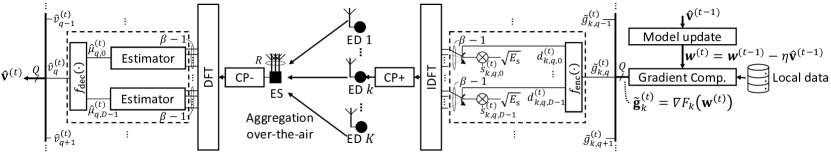
Figure 1: The transmitter and receiver diagrams with the proposed OAC scheme for FEEL.

III-C MSE Analysis

The variable $\lVert\textbf{r}_{m_{i,\ell},l_{i,\ell}}^{(\mathscr{t})}\rVert_{2}^{2}/R$ in (15) is the average of $R$ exponential variables with the mean $E_{\rm s}U_{q,i,\ell}+\sigma_{\rm n}^{2}$. Thus, the distribution of $\lVert\textbf{r}_{m_{i,\ell},l_{i,\ell}}^{(\mathscr{t})}\rVert_{2}^{2}/R$ is $\Gamma({R,R/(E_{\rm s}U_{q,i,\ell}+\sigma_{\rm n}^{2})})$. As a result, the mean and the variance of the estimator $\hat{U}_{q,i,\ell}$ can be calculated via the properties of a gamma distribution as

$${\mathbb{E}}\left[\hat{U}_{q,i,\ell}\right]=\frac{{\mathbb{E}}\left[\lVert\textbf{r}_{m_{i,\ell},l_{i,\ell}}^{(\mathscr{t})}\rVert_{2}^{2}/R\right]}{E_{\rm s}}-\frac{\sigma_{\rm n}^{2}}{E_{\rm s}}=U_{q,i,\ell}~{},$$ (18)

and

$$\textrm{var}\left(\hat{U}_{q,i,\ell}\right)=\frac{\textrm{var}\left(\lVert\textbf{r}_{m_{i,\ell},l_{i,\ell}}^{(\mathscr{t})}\rVert_{2}^{2}/R\right)}{E_{\rm s}}=\frac{1}{R}\left(U_{q,i,\ell}+\frac{\sigma_{\rm n}^{2}}{E_{\rm s}}\right)^{2}~{},$$ (19)

respectively, where the expectation is calculated over the randomness of the channel and noise. Hence, $\hat{U}_{q,i,\ell}$ is an unbiased estimator. Also, based on (16) and (17), both $\hat{\mu}_{{q},{i}}^{(\mathscr{t})}$ and ${\hat{v}}^{(\mathscr{t})}_{q}$ are unbiased estimators of $\mu_{{q},{i}}^{(\mathscr{t})}$ and ${\bar{v}}^{(\mathscr{t})}_{q}$, respectively. For a given $\{U_{q,i,\ell}|\ell\in\mathbb{Z}_{\beta-1}\}$, by using (16) and (19), the variance of the estimator $\hat{\mu}_{{q},{i}}^{(\mathscr{t})}$ is obtained as

$$\textrm{var}\left({\hat{\mu}_{{q},{i}}^{(\mathscr{t})}}\right)=\frac{1}{RK^{2}}\sum_{\ell=0}^{\beta-2}a_{\ell}^{2}\left(U_{q,i,\ell}+\frac{\sigma_{\rm n}^{2}}{E_{\rm s}}\right)^{2}~{}.$$ (20)

Thus, we can calculate the variance of the estimator ${{{\hat{v}}^{(\mathscr{t})}_{q}}}$ as

$$\textrm{var}\left({{\hat{v}}^{(\mathscr{t})}_{q}}\right)=\frac{v_{\rm max}^{2}}{\xi^{2}RK^{2}}\sum_{i=0}^{D-1}\sum_{\ell=0}^{\beta-2}a_{\ell}^{2}\left(U_{q,i,\ell}+\frac{\sigma_{\rm n}^{2}}{E_{\rm s}}\right)^{2}\beta^{2i}~{}.$$ (21)

Hence, the MSE of the estimator ${\hat{v}}^{(\mathscr{t})}_{q}$ can be obtained as

$${{\text{MSE}}}\left({\hat{v}}^{(\mathscr{t})}_{q}\right)=$$

$$\frac{v_{\rm max}^{2}}{\xi^{2}RK^{2}}\sum_{i=0}^{D-1}\sum_{\ell=0}^{\beta-2}a_{\ell}^{2}\left(U_{q,i,\ell}+\frac{\sigma_{\rm n}^{2}}{E_{\rm s}}\right)^{2}\beta^{2i}+\underbrace{\frac{1}{K^{2}}\left(\sum_{k=0}^{K-1}{\bar{\tilde{g}}}_{k,q}^{(\mathscr{t})}-{\tilde{g}}_{k,q}^{(\mathscr{t})}\right)^{2}}_{({v}^{(\mathscr{t})}_{q}-{\bar{v}}^{(\mathscr{t})}_{q})^{2}}~{},$$

where the last term is the squared bias due to the quantization error. From the MSE, we can infer that the error rapidly diminishes either by increasing $\beta$ and $D$, at a cost of increased number of resources, or increasing $K$.

IV Numerical Results

To numerically analyze OAC with the proposed scheme for FEEL, we consider the learning task of handwritten-digit recognition in a single cell with $K=25$ EDs. We set the SNR, i.e., $1/\sigma_{\rm n}^{2}$, to be $20$ dB, and choose the number of antennas at the ES as $R\in\{1,25\}$. For the fading channel, we consider ITU Extended Pedestrian A (EPA) with no mobility and regenerate the channels between the ES and the EDs independently for each communication round to capture the long-term channel variations. The subcarrier spacing is set to $15$ kHz. We use $M=1200$ subcarriers (i.e., the signal bandwidth is $18$ MHz). Hence, the difference between time of arriving ED signals is maximum $T_{\rm sync}=55.6$ ns. We assume that the synchronization uncertainty at the ES is $N_{\text{err}}=3$ samples. For the comparisons, we consider FSK-MV proposed in [15] as it is based on a non-coherent detection and provides robustness against time-synchronization errors. We do not consider methods based on precoding such as TCI since their performance can deteriorate quickly in the cases of time-synchronization errors [16, 15] or imperfect CSI [14]. We consider $\beta\in\{3,5,7\}$ and $D=\{1,2\}$.

For the local data at the EDs, we use the MNIST database that contains labeled handwritten-digit images size of $28\times 28$ from digit 0 to digit 9. We distribute the data samples in the MNIST database to the EDs to generate representative results for FEEL. We consider both homogeneous and heterogeneous data distributions in the cell. To prepare the data, we first choose $|\mathcal{D}|=25000$ training images from the database, where each digit has distinct $2500$ images. For the scenario with the homogeneous data distribution, we assume that each ED has $250$ distinct images for each digit. As done in [15], for the scenario with the heterogeneous data distribution, we divide the cell into 5 areas with concentric circles and the EDs located in $u$th area have the data samples with the labels $\{u-1,u,1+u,2+u,3+u,4+u\}$ for $u\in\{1,\hbox to10.00002pt{.\hss.\hss.},5\}$ (See [15, Figure 3] for an illustration). The number of EDs in each area is $5$. As discussed in Section II, we assume that the path loss is compensated through a power control mechanism. For the model, we consider a convolution neural network (CNN) given in [15, Table 1]. At the input layer, standard normalization is applied to the data. Our model has $Q=123090$ learnable parameters. For the update rule, the learning rate is set to $0.001$. The batch size $n_{\rm b}$ is $64$. For the proposed scheme, we use SGD with the momentum $0.9$. For the test accuracy, we use $10000$ test samples available in the MNIST database.

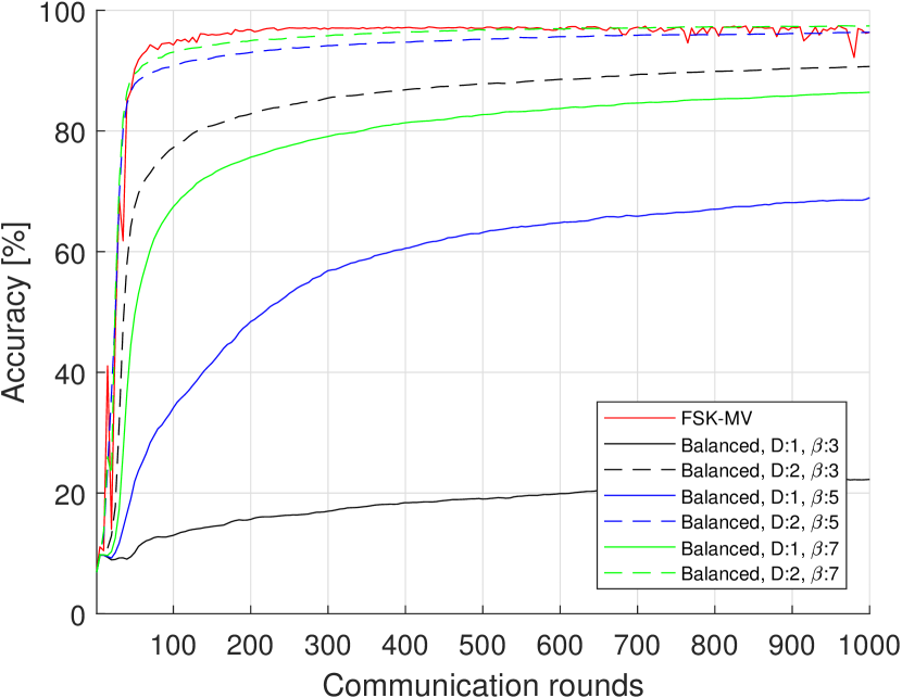
(a) $R=1$.

(b) $R=25$.

Figure 2: Test accuracy (Homogeneous data distribution).

In Figure 2, we provide the test accuracy versus communication rounds for the scenario with homogeneous data distribution. In Figure 2LABEL:sub@subfig:acc_homo_R1_wM_woAAM, there is only a single antenna at the ES. Although the accuracy results with the proposed scheme improve for larger $\beta$ or $D$ (i.e., less $\sigma_{\rm channel}^{2}$) for this scenario, the FSK-MV is superior to the proposed scheme in terms of convergence rate. This is because FSK-MV is based on signSGD, while the proposed scheme implements SGD. In [17], it was also mentioned that signSGD can outperform SGD by providing stronger weight to the gradient direction as compared to SGD when the gradients are noisy. In Figure 2LABEL:sub@subfig:acc_homo_R25_wM_woAAM, we set the number of antennas at the ES to be $25$. Although this improves the MSE considerably, its impact on the test accuracy is almost negligible. Hence, the proposed scheme can achieve notable test accuracy results even when there is only a single antenna at the ES.

In Figure 3, the test accuracy is evaluated when the data distribution is highly heterogeneous, i.e., each ED has only 6 unique digits. We use the same parameters used for Figure 2. In this case, the performance of the FSK-MV degrades drastically, whereas the performance of the proposed scheme is similar to one in Figure 2. The test accuracy under heterogeneous data distribution is less than 80% for the FSK-MV (this is also reported in [15]). On the other hand, the proposed scheme with a larger set of $\beta$ and $D$ can achieve more than 90% test accuracy as shown in Figure 3LABEL:sub@subfig:acc_heto_R1_wM_woAAM for $R=1$. A similar observation can also be made for $R=25$ as in Figure 3LABEL:sub@subfig:acc_heto_R25_wM_woAAM, i.e., it can provide high accuracy, up to 98%, even when the data distribution is not homogeneous.

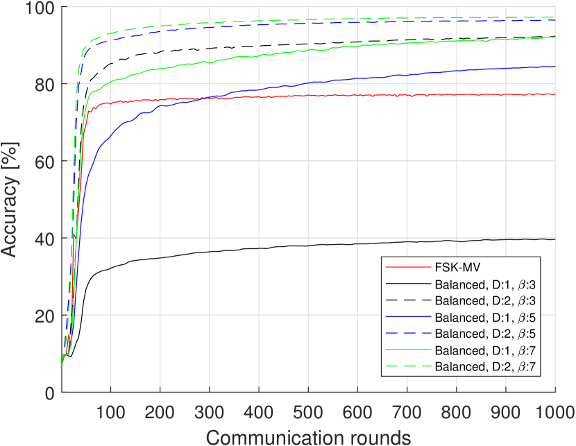
(a) $R=1$.

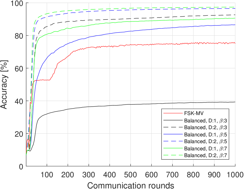
(b) $R=25$.

Figure 3: Test accuracy (Heterogeneous data distribution).

V Concluding Remarks

In this study, we investigate an OAC method that exploits balanced number systems for gradient aggregation. The proposed scheme achieves a continuous-valued computation through a digital scheme by exploiting the fact that the average of the numerals in the real domain can be used to compute the average of the corresponding real-valued parameters approximately. With the proposed OAC method, the local stochastic gradients are encoded into a sequence where the elements of the sequence determine the activated OFDM subcarriers. We also use a non-coherent receiver to eliminate the precise sample-level time synchronization and channel estimation overhead due to the channel inversion techniques. We show that the proposed scheme results in a lower MSE at the expense of more resources. Future work will present the corresponding convergence analysis.

References

• [1] B. Nazer and M. Gastpar, “Computation over multiple-access channels,” IEEE Trans. Inf. Theory, vol. 53, no. 10, pp. 3498–3516, Oct. 2007.
• [2] M. Gastpar and M. Vetterli, “Source-channel communication in sensor networks,” in Proc. International Conference on Information Processing in Sensor Networks (IPSN).   Berlin, Heidelberg: Springer-Verlag, 2003, p. 162–177.
• [3] M. Goldenbaum, H. Boche, and S. Stańczak, “Harnessing interference for analog function computation in wireless sensor networks,” IEEE Trans. Signal Process., vol. 61, no. 20, pp. 4893–4906, Oct. 2013.
• [4] W. Liu, X. Zang, Y. Li, and B. Vucetic, “Over-the-air computation systems: Optimization, analysis and scaling laws,” IEEE Trans. Wireless Commun., vol. 19, no. 8, pp. 5488–5502, Aug. 2020.
• [5] M. Chen, D. Gündüz, K. Huang, W. Saad, M. Bennis, A. V. Feljan, and H. Vincent Poor, “Distributed learning in wireless networks: Recent progress and future challenges,” IEEE J. Sel. Areas Commun., pp. 1–26, 2021.
• [6] P. Park, P. Di Marco, and C. Fischione, “Optimized over-the-air computation for wireless control systems,” IEEE Commun. Lett, vol. 26, no. 2, pp. 1–5, 2022.
• [7] B. McMahan, E. Moore, D. Ramage, S. Hampson, and B. A. y. Arcas, “Communication-Efficient Learning of Deep Networks from Decentralized Data,” in Proc. International Conference on Artificial Intelligence and Statistics, A. Singh and J. Zhu, Eds., vol. 54.   PMLR, 20–22 Apr 2017, pp. 1273–1282.
• [8] M. Chen, Z. Yang, W. Saad, C. Yin, H. V. Poor, and S. Cui, “A joint learning and communications framework for federated learning over wireless networks,” IEEE Trans. Wireless Commun., vol. 20, no. 1, pp. 269–283, 2021.
• [9] G. Zhu, Y. Wang, and K. Huang, “Broadband analog aggregation for low-latency federated edge learning,” IEEE Trans. Wireless Commun., vol. 19, no. 1, pp. 491–506, Jan. 2020.
• [10] T. Sery, N. Shlezinger, K. Cohen, and Y. C. Eldar, “Over-the-air federated learning from heterogeneous data,” IEEE Transactions on Signal Processing, vol. 69, pp. 3796–3811, 2021.
• [11] M. M. Amiri and D. Gündüz, “Federated learning over wireless fading channels,” IEEE Trans. Wireless Commun., vol. 19, no. 5, pp. 3546–3557, Feb. 2020.
• [12] G. Zhu, Y. Du, D. Gündüz, and K. Huang, “One-bit over-the-air aggregation for communication-efficient federated edge learning: Design and convergence analysis,” IEEE Trans. Wireless Commun., vol. 20, no. 3, pp. 2120–2135, Nov. 2021.
• [13] N. Zhang and M. Tao, “Gradient statistics aware power control for over-the-air federated learning,” IEEE Trans. Wireless Commun., vol. 20, no. 8, pp. 5115–5128, 2021.
• [14] H. Jung and S.-W. Ko, “Performance analysis of UAV-enabled over-the-air computation under imperfect channel estimation,” IEEE Wireless Commun. Lett., pp. 1–1, Nov. 2021.
• [15] A. Şahin, B. Everette, and S. Hoque, “Distributed learning over a wireless network with FSK-based majority vote,” in Proc. IEEE International Conference on Advanced Communication Technologies and Networking (CommNet), Dec. 2021, pp. 1–9.
• [16] ——, “Over-the-air computation with DFT-spread OFDM for federated edge learning,” in Proc. IEEE Wireless Communications and Networking Conference (WCNC), Apr. 2022, pp. 1–6.
• [17] J. Bernstein, Y.-X. Wang, K. Azizzadenesheli, and A. Anandkumar, “signSGD: Compressed optimisation for non-convex problems,” in Proc. in International Conference on Machine Learning, vol. 80.   Proceedings of Machine Learning Research, 10–15 Jul 2018, pp. 560–569.
• [18] I. Koren, Computer Arithmetic Algorithms, 2nd ed.   A K Peters/CRC Press, 2018.
• [19] G. H. Hardy and E. M. Wright, An Introduction to the Theory of Numbers, 6th ed.   Oxford, 2008.
• [20] P. Liu, J. Jiang, G. Zhu, L. Cheng, W. Jiang, W. Luo, Y. Du, and Z. Wang, “Training time minimization for federated edge learning with optimized gradient quantization and bandwidth allocation,” Front Inform Technol Electron Eng, vol. 23, no. 8, pp. 1247–1263, 2022.