Efficient variational approach to the Fermi polaron problem in two dimensions,
both in and out of equilibrium

Abstract

We develop a non-Gaussian variational approach that enables us to study both equilibrium and far-from-equilibrium physics of the two-dimensional Fermi polaron. This method provides an unbiased analysis of the polaron-to-molecule phase transition without relying on truncations in the total number of particle-hole excitations. Our results – which include the ground state energy and quasiparticle residue – are in qualitative agreement with the known Monte Carlo calculations. The main advantage of the non-Gaussian states compared to conventional numerical methods is that they enable us to explore long-time polaron evolution and, in particular, study various spectral properties accessible to both solid-state and ultracold atom experiments. We design two types of radiofrequency spectroscopies to measure polaronic and molecular spectral functions. Depending on the parameter regime, we find that these spectral functions and fermionic density profiles near the impurity display either long-lived oscillations between the repulsive and attractive polaron branches or exhibit fast relaxational dynamics to the molecular state.

I Introduction

Fermi polaron models correspond to a general class of quantum many-body problems in which a single impurity interacts with a bath of fermions. Historically, theoretical work in this area started with the analysis of models with infinitely heavy impurities, which exhibit a phenomenon of orthogonality catastrophe [1]. The latter is an observation of P. W. Anderson that even a weak impurity potential results in the creation of an infinite number of low-energy particle-hole excitations. Orthogonality catastrophe plays an important role in several areas of physics, including X-ray scattering [2, 3], photoemission [4, 5, 6], transport in mesoscopic systems [7, 8], and radiofrequency (RF) and Rydberg spectroscopies in ultracold atoms [9, 10, 11, 12]. Dynamics in polaronic systems becomes even richer when impurity particles are endowed with internal degrees of freedom. The simplest example is adding spin states to a localized impurity, corresponding to the Kondo model. This class of systems exhibits such striking phenomena as non-monotonic temperature dependence of resistivity in metals with magnetic impurities [13], formation of heavy fermion materials [14], and even emergence of non-Fermi liquid states [15, 16].

Another way of enriching impurity dynamics is to make them mobile. Models of mobile Fermi polarons were first considered in the context of He⁴/He³ mixtures, ions in the normal liquid of He³, and diffusion of muons in metals [17]. In comparison to the infinitely heavy impurity models, a new feature of such systems comes from the finite recoil energy of the impurity particle. This appears as a constraint on the scattering processes of the bath fermions and raises the question of whether the states with and without the impurity-bath coupling are orthogonal to each other. For infinitely heavy impurities, we have the orthogonality catastrophe, which means that the two states are orthogonal, while for heavy but finite mass impurities, the answer was argued to depend on dimensionality [18]. In two- and three-dimensional systems, the two states are expected to have a finite overlap, which in turn implies a finite quasiparticle weight, whereas in one-dimensional systems, the quasiparticle weight can be proven to vanish [19, 20].

It is interesting to note, however, that developing accurate theoretical models for describing properties of mobile impurities interacting with a Fermi bath remains a considerable theoretical challenge. Earlier studies of mobile Fermi polarons have been motivated by two primary considerations. On the one hand, they provided a concrete example of the emergence of friction in a purely quantum-mechanical system [21, 22]. On the other hand, the issue of quasiparticle weight was considered as a paradigmatic case study of the concept of quasiparticles in strongly interacting Fermi systems.

Renewed interest in the study of Fermi polarons came with the progress of experiments in the field of ultracold atoms. These systems make it possible to realize Fermi polarons with different mass ratios of the impurity and bath particles and tune impurity-bath interaction strength using magnetic Feshbach resonances [9, 23, 10, 24, 25, 26, 27, 28, 29]. The tunability of microscopic interactions brings a new feature of the interplay of few- and many-body aspects of the problem. In particular, Feshbach resonance itself corresponds to the appearance of a bound state in a two-body problem [30]. An interesting question then is whether one finds a transition between molecular and polaronic ground states in a many-body system. In the former case, the impurity atom makes a bound state with one of the bath fermions, accompanied by the vanishing quasiparticle weight. In the polaronic case, the impurity interacts with many bath particles and forms a state that has finite quasiparticle weight. In three-dimensional systems, there is strong numerical [31, 32] and experimental [9] evidence for the polaron-to-molecule transition. Notably, one finds that in the case of equal masses of impurity and bath particles, one can obtain a good description of many-body polaronic states by including only a single particle-hole excitation [33]. These so-called Chevy ansatz (CA) wave functions work surprisingly well even at unitarity when the scattering length diverges [34, 35]. In two-dimensional (2D) systems, analysis based on CA suggested that the ground state should always be of the polaronic type [36] (for equal masses of the impurity and bath fermions). However, analysis that extended CA to include two particle-hole excitations supported the existence of the polaron-to-molecule transition [37, 38, 39, 40].

The most recent addition to the experimental platforms for exploring Fermi polarons utilizes excitons and electrons (or holes) in transition metal dichalcogenides (TMDs) [41]. In contrast to traditional Si and GaAs semiconductors, TMDs have a smaller dielectric constant and heavier electron mass, resulting in much stronger binding energy and smaller size of an exciton. For a broad range of electron densities used in experiments, the size of excitons is much smaller than a typical inter-electron distance. Hence excitons can be treated as impurities when analyzing their interaction with electrons. Furthermore, there is an effective Feshbach resonance between electrons and excitons, which manifests itself in the repulsive and attractive branches in the absorption spectra. These branches are strongly reminiscent of the Fermi polaron spectra measured in two-dimensional systems of ultracold fermions [41, 42, 43, 44].

Motivated by these developments, we set ourselves a goal of developing an efficient theoretical formalism for describing Fermi polarons in 2D systems, both in and out of equilibrium. The approach we choose here is based on the non-Gaussian states detailed in Ref. [45]. These variational states do not rely on truncations in the number of particle-hole excitations. As such, this approach provides an unbiased analysis of the competition between polaronic and molecular states. It also guarantees that in the limit of infinitely heavy impurities, our solution reduces to the exact one based on the Functional Determinant Approach [46, 47, 48]. Additional motivation to employ the non-Gaussian states is that they capture remarkably well the physics of 1D Fermi polaron [49, 50, 51, 52, 53, 54, 55, 20]. The main advantage of our method is the possibility of analyzing non-equilibrium properties [47, 56, 57, 48, 54, 58, 59, 60, 61] of polaronic systems, including various spectral functions. As part of our analysis, we introduce here new characteristics of Fermi-polaron systems, namely: molecular residue and molecular spectral function. These quantities provide a complementary perspective on the polaron-to-molecule transition. We discuss how they can be measured in experiments with ultracold atoms.

This paper is organized as follows: In Sec. II, we introduce the general non-Gaussian approach, which includes the ground-state optimization via the imaginary-time evolution, the study of the real-time dynamics by projecting the Schrödinger equation on the variational manifold, and the linear-response analysis by linearizing the equations of motion around the ground-state configuration. In Sec. III, a first-order polaron-to-molecule transition is identified, where both the ground-state energy and single-particle residue are in excellent agreement with those from CA and diagrammatic Monte Carlo (DMC) calculations. Section IV is dedicated to far-from-equilibrium dynamics of the polaronic system. There, we compute various spectral properties and introduce two types of RF spectroscopies to quantify the polaron-to-molecule transition. The spectral functions exhibit distinctive dynamical behaviors in the polaronic and molecular phases, such as long-lived oscillations between the repulsive and attractive polarons and fast relaxation to the molecular state from different initial states. Finally, the main results are briefly summarized in Sec. V.

II Formalism

This section introduces the non-Gaussian formalism to study the Fermi polaron in two spatial dimensions. In the first subsection, we formulate the model of a single impurity in the 2D Fermi gas and apply the Lee-Low-Pines (LLP) transformation [62] that decouples the impurity from the fermionic degrees of freedom. We then, in the second subsection, introduce the non-Gaussian variational states, which allow us to investigate the ground-state properties and the real-time dynamics. Up to this stage, our framework closely follows that used in Ref. [20] to study the one-dimensional Fermi polaron. The two-dimensional problem is much more challenging due to the large number of the involved degrees of freedom. Consequently, numerical simulations are limited to small system sizes. To overcome this issue, in the third subsection, we utilize the rotational symmetry of the problem, which in turn allows us to efficiently model even relatively large systems. The fourth subsection is dedicated to the linear response theory within the formalism of the non-Gaussian states.

II.1 Model

A single mobile impurity immersed in a 2D Fermi gas is described via the following microscopic Hamiltonian:

$$H=H_{\mathrm{b}}+H_{\mathrm{imp}}+H_{\mathrm{int}},$$ (1)

where

$$H_{\mathrm{b}}=-\frac{1}{2m_{\mathrm{b}}}\int d^{2}x\,\hat{\Psi}^{\dagger}(\mathbf{x})\nabla^{2}\hat{\Psi}(\mathbf{x})$$ (2)

represents the kinetic energy of the fermionic bath. The kinetic energy of the impurity is given by:

$$H_{\mathrm{imp}}=-\frac{1}{2m_{\mathrm{imp}}}\int d^{2}x\,\hat{\Psi}_{\mathrm{imp}}^{\dagger}(\mathbf{x})\nabla^{2}\hat{\Psi}_{\mathrm{imp}}(\mathbf{x}).$$ (3)

The contact interaction term reads:

$$H_{\mathrm{int}}=g\int d^{2}x\,\hat{\Psi}^{\dagger}(\mathbf{x})\hat{\Psi}(\mathbf{x})\hat{\Psi}_{\mathrm{imp}}^{\dagger}(\mathbf{x})\hat{\Psi}_{\mathrm{imp}}(\mathbf{x}),$$ (4)

where $\hat{\Psi}(\mathbf{x})$ and $\hat{\Psi}^{\dagger}(\mathbf{x})$ ($\hat{\Psi}_{\mathrm{imp}}(\mathbf{x})$ and $\hat{\Psi}_{\mathrm{imp}}^{\dagger}(\mathbf{x})$) denote the fermionic (impurity) creation and annihilation operators, respectively; they obey the fermionic anti-commutation relations. Here $m_{\mathrm{b}}$ and $m_{\mathrm{imp}}$ are the fermion and impurity masses, respectively. In the 2D gas, the attractive interaction strength $g$ is related to the 2D scattering length $a_{\mathrm{2D}}$ via the Lippmann-Schwinger equation:

$$\frac{1}{g}=-\frac{1}{L^{2}}\sum_{|\mathbf{k}|<k_{\Lambda}}\frac{1}{E_{B}+k^{2}/(2m_{\mathrm{r}})},$$ (5)

where $E_{B}=1/(2m_{\mathrm{r}}a_{\mathrm{2D}}^{2})$ is the binding energy of the weakly bound diatomic molecule, $m_{\mathrm{r}}=m_{\mathrm{b}}m_{\mathrm{imp}}/(m_{\mathrm{b}}+m_{\mathrm{imp}})$ denotes the reduced mass, $L$ is the linear system’s size, and $k_{\Lambda}$ is the ultraviolet (UV) momentum cutoff. In momentum space, the Hamiltonian reads:

$$H= \sum_{\mathbf{k}}(\varepsilon_{\mathrm{b},\mathbf{k}}c_{\mathbf{k}}^{\dagger}c_{\mathbf{k}}+\varepsilon_{\mathrm{imp},\mathbf{k}}f_{\mathbf{k}}^{\dagger}f_{\mathbf{k}})$$

$$+\frac{g}{L^{2}}\sum_{\mathbf{k},\mathbf{p},\mathbf{q}}f_{\mathbf{k}}^{\dagger}f_{\mathbf{k}+\mathbf{q}}c_{\mathbf{p}}^{\dagger}c_{\mathbf{p-q}},$$ (6)

where $\varepsilon_{\sigma=\mathrm{b,imp},\mathbf{k}}=k^{2}/(2m_{\sigma})$ and $\mathbf{k}=2\pi(n_{x},n_{y})/L$ with integer $n_{x}$ and $n_{y}$.

We turn to discuss the Lee-Low-Pines (LLP) transformation $U_{\mathrm{LLP}}=e^{-i\mathbf{Q}_{b}\cdot\mathbf{X}_{\mathrm{imp}}}$, which allows one to simplify the model by eliminating the impurity degrees of freedom. This unitary transformation relies on the very fact of the total momentum conservation $[\mathbf{Q}_{\mathrm{tot}},H]=0$, where $\mathbf{Q}_{\mathrm{tot}}=\mathbf{Q}_{\mathrm{imp}}+\mathbf{Q}_{\mathrm{b}}$. Here $\mathbf{Q}_{\mathrm{imp}}=\sum_{\mathbf{k}}\mathbf{k}f_{\mathbf{k}}^{\dagger}f_{\mathbf{k}}$ and $\mathbf{Q}_{\mathrm{b}}=\sum_{\mathbf{k}}\mathbf{k}c_{\mathbf{k}}^{\dagger}c_{\mathbf{k}}$ represent the momenta of the impurity and the fermi bath, respectively. We also defined $\mathbf{X}_{\mathrm{imp}}=\int d^{2}x\,\mathbf{x}\,\hat{\Psi}_{\mathrm{imp}}^{\dagger}(\mathbf{x})\hat{\Psi}_{\mathrm{imp}}(\mathbf{x})$ to be the impurity position operator. Physically, the LLP transformation simply encodes the fact that the impurity momentum $\mathbf{Q}_{\mathrm{imp}}=U_{\mathrm{LLP}}^{\dagger}\mathbf{Q}_{\mathrm{tot}}U_{\mathrm{LLP}}$ can be reconstructed from the total momentum $\mathbf{Q}_{\mathrm{tot}}$ and the net momentum $\mathbf{Q}_{\mathrm{b}}$ of the host fermions. Under the LLP transformation, the system is transformed into the co-moving frame of the impurity. The modified Hamiltonian $H_{\mathrm{LLP}}=U_{\mathrm{LLP}}^{\dagger}HU_{\mathrm{LLP}}$ in the single-impurity subspace $\sum_{\mathbf{k}}f_{\mathbf{k}}^{\dagger}f_{\mathbf{k}}=1$ then reads:

$$H_{\mathrm{LLP}}= \sum_{\mathbf{k}}(\varepsilon_{\mathrm{b},\mathbf{k}}c_{\mathbf{k}}^{\dagger}c_{\mathbf{k}}+\varepsilon_{\mathrm{imp},\mathbf{k-Q}_{\mathrm{b}}}f_{\mathbf{k}}^{\dagger}f_{\mathbf{k}})$$

$$+\frac{g}{L^{2}}\sum_{\mathbf{k}}f_{\mathbf{k}}^{\dagger}f_{\mathbf{k}}\sum_{\mathbf{p},\mathbf{q}}c_{\mathbf{p}}^{\dagger}c_{\mathbf{q}}.$$ (7)

We note that in the transformed frame, $f_{\mathbf{k}}^{\dagger}f_{\mathbf{k}}$ commutes with $H_{\mathrm{LLP}}$; in other words, $\mathbf{Q}_{\mathrm{imp}}=\mathbf{K}_{0}$ becomes an integral of motion in the co-moving frame so that the LLP Hamiltonian can be written as:

$$H_{\mathrm{LLP}}=\sum_{\mathbf{k}}\varepsilon_{\mathrm{b},\mathbf{k}}c_{\mathbf{k}}^{\dagger}c_{\mathbf{k}}+\frac{g}{L^{2}}\sum_{\mathbf{k},\mathbf{p}}c_{\mathbf{k}}^{\dagger}c_{\mathbf{p}}+\varepsilon_{\mathrm{imp},\mathbf{K}_{0}\mathbf{-Q}_{\mathrm{b}}}.$$ (8)

We obtain that the impurity degrees of freedom are eliminated at the price of introducing a non-local impurity-mediated interaction between the fermions, encoded in the third term of Eq. (8).

II.2 Non-Gaussian variational approach

To study the polaron physics, both in and out of equilibrium, we employ the non-Gaussian family of variational wave functions. Specifically, guided by the LLP transformation, we write the many-body polaronic state in the laboratory frame as:

$$|\Psi_{\mathbf{K}_{0}}\rangle=U_{\mathrm{LLP}}f_{\mathbf{K}_{0}}^{\dagger}|0\rangle_{\mathrm{imp}}\otimes|\Psi_{\mathrm{GS}}\rangle.$$ (9)

Implicit in Eq. (9) is that the state $|\Psi_{\mathrm{GS}}\rangle$ represents the fermionic wave function in the co-moving frame. We then choose $|\Psi_{\mathrm{GS}}\rangle$ to be Gaussian [45, 20]:

$$|\Psi_{\mathrm{GS}}\rangle=U_{\mathrm{GS}}|\mathrm{FS}\rangle=e^{-i\theta}e^{ic^{\dagger}\xi c}|\mathrm{FS}\rangle,$$ (10)

where $|\mathrm{FS}\rangle$ describes the Fermi sea set by a Fermi momentum $k_{F}$. At this stage, our variational parameters are the global phase $\theta$ and Hermitian matrix $\xi$ written in the Dirac basis $c=\left(c_{\mathbf{k}_{1}},c_{\mathbf{k}_{2}},\ldots,c_{\mathbf{k}_{N}}\right)^{\mathrm{T}}$, with $N$ being the total number of fermionic degrees of freedom. We note that even though the wave function in the co-moving frame is factorizable between the impurity and host fermions, it is highly entangled by $U_{\mathrm{LLP}}$ when expressed in the laboratory frame, cf. Eq. (9).

Any variational state applied to many-body problems represents some approximation. Given that often there are no small parameters or exact solutions, it is crucial to test the validity of any such variational approach. For the 1D Fermi polaron, it was demonstrated in Ref. [20] that the non-Gaussian states of the form (9) reproduce the exact Bethe ansatz results, both in and out of equilibrium. The validity of the non-Gaussian wave functions in the 2D polaron problem is the subject of the next sections.

To optimize for the best variational wave function that approximates the ground state, we employ the imaginary-time dynamics. For now, instead of $\theta$ and $\xi$, it is more convenient to work with the covariance matrix

$$\Gamma_{ij}\equiv\langle\Psi_{\mathrm{GS}}|c_{i}^{\dagger}c_{j}|\Psi_{\mathrm{GS}}\rangle=U^{\ast}\Gamma_{\mathrm{FS}}U^{\mathrm{T}},$$ (11)

where $\Gamma_{\mathrm{FS}}$ is the covariance matrix of the Fermi sea and $U=e^{i\xi}$. Then the projection of the imaginary-time evolution onto the tangential space of the variational manifold gives rise to [45]:

$$\partial_{\tau}\Gamma=-\mathcal{H}_{\mathrm{MF}}^{\mathrm{T}}\Gamma-\Gamma\mathcal{H}_{\mathrm{MF}}^{\mathrm{T}}+2\Gamma\mathcal{H}_{\mathrm{MF}}^{\mathrm{T}}\Gamma.$$ (12)

Here we employed Wick’s theorem to derive the mean-field Hamiltonian

$$(\mathcal{H}_{\mathrm{MF}})_{\mathbf{kp}}= \left(\frac{k^{2}}{2m_{\mathrm{r}}}\mathbf{-}\frac{\mathbf{K}_{0}\cdot\mathbf{k}}{m_{\mathrm{imp}}}\right)\delta_{\mathbf{kp}}+\frac{g}{L^{2}}$$ (13)

$$+\frac{1}{m_{\mathrm{imp}}}\left(\left\langle\mathbf{Q}_{\mathrm{b}}\right\rangle_{\mathrm{GS}}\cdot\mathbf{k}\,\delta_{\mathbf{kp}}-\mathbf{k\cdot p}\left\langle c_{\mathbf{p}}^{\dagger}c_{\mathbf{k}}\right\rangle_{\mathrm{GS}}\right).$$

For the imaginary-time evolution, the global phase $\theta$ can be chosen arbitrarily, and the variational energy

$$E_{\mathbf{K}_{0}}= \mathrm{Tr}(\mathcal{H}_{\mathrm{MF}}\Gamma^{\mathrm{T}})+\frac{1}{2m_{\mathrm{imp}}}\Big{(}K_{0}^{2}+\left\langle\mathbf{Q}_{\mathrm{b}}\right\rangle^{2}_{\mathrm{GS}}$$

$$-\sum_{\mathbf{kp}}\mathbf{k\cdot p}\langle c_{\mathbf{k}}^{\dagger}c_{\mathbf{p}}\rangle_{\mathrm{GS}}\langle c_{\mathbf{p}}^{\dagger}c_{\mathbf{k}}\rangle_{\mathrm{GS}}\Big{)}$$ (14)

decreases monotonically and reaches its ground-state value in the limit $\tau\rightarrow\infty$.

The real-time equations of motion are derived from Dirac’s variational principle, with the result [20]:

$$\partial_{t}U = -i\mathcal{H}_{\mathrm{MF}}U,$$ (15)

$$\partial_{t}\theta = E_{\mathbf{K}_{0}}-\mathrm{Tr}\left(\mathcal{H}_{\mathrm{MF}}\Gamma^{\mathrm{T}}\right).$$ (16)

From this, one can get an equation solely on the covariance matrix:

$$i\partial_{t}\Gamma=\Gamma\mathcal{H}_{\mathrm{MF}}^{\mathrm{T}}-\mathcal{H}_{\mathrm{MF}}^{\mathrm{T}}\Gamma.$$ (17)

This result could alternatively be derived from projecting the Schrödinger equation onto the tangential space of the variational manifold [45].

As a remark, we note that during either the imaginary-time or real-time evolution, the total number of fermions is conserved $d_{\tau,t}N_{f}{=0}=d_{\tau,t}\mathrm{Tr}(\Gamma)=0$. This follows from the fact that provided the initial state is pure, as encoded in $\Gamma^{2}=\Gamma$, it will remain pure upon the evolution.

II.3 Rotational symmetry

Let us consider the situation with zero total momentum $\mathbf{K}_{0}=\mathbf{0}$, where the system is rotationally invariant. When performing the LLP transformation for this case, we work with continuous rather than discretized variables, as in Eqs. (1)-(4). The rotational symmetry implies that the covariance matrix $\Gamma_{\mathbf{pp}^{\prime}}$ (or any other observable) depends only on $p$, $p^{\prime}$, and the relative angle $\vartheta-\vartheta^{\prime}$, which allows us to write:

$$\Gamma_{\mathbf{pp}^{\prime}}=\frac{1}{2\pi\delta_{p}\sqrt{pp^{\prime}}}\sum_{n}\Gamma_{pp^{\prime}}^{n}e^{-in(\vartheta-\vartheta^{\prime})}.$$ (18)

In this expression, the radial momenta $p$ and $p^{\prime}$ in each of the matrices $\Gamma_{pp^{\prime}}^{n}$ have been discretized with spacing $\delta_{p}$. Here, $\Gamma_{pp^{\prime}}^{n}$ is understood as the following covariance matrix:

$$\Gamma_{pp^{\prime}}^{n}=\langle\Psi_{\mathrm{GS}}|c_{p}^{n\dagger}c_{p^{\prime}}^{n}|\Psi_{\mathrm{GS}}\rangle,$$ (19)

where $c_{p}^{n}\propto\int d\vartheta\,c_{\mathbf{p}}e^{-in\vartheta}$ satisfing $[c_{p}^{n},c_{p^{\prime}}^{n\dagger}]=\delta_{pp^{\prime}}$ is the annihilation operator in the angular momentum basis. The imaginary-time equations of motion now read:

$$\partial_{\tau}\Gamma^{n}=-[\mathcal{H}^{n}]^{\mathrm{T}}\Gamma^{n}-\Gamma^{n}[\mathcal{H}^{n}]^{\mathrm{T}}+2\Gamma^{n}[\mathcal{H}^{n}]^{\mathrm{T}}\Gamma^{n},$$ (20)

where the mean-field Hamiltonian in the angular momentum channel $n$ is given by:

$$\mathcal{H}_{pp^{\prime}}^{n}= \frac{p^{2}}{2m_{\mathrm{r}}}\delta_{pp^{\prime}}+\frac{g\delta_{p}\sqrt{pp^{\prime}}}{2\pi}\delta_{n0}$$

$$-\frac{pp^{\prime}}{2m_{\mathrm{imp}}}\left(\Gamma_{p^{\prime}p}^{n+1}+\Gamma_{p^{\prime}p}^{n-1}\right).$$ (21)

As encoded in the second term in Eq. (21), the impurity induces a potential in the zero angular momentum channel only – this is because we consider contact coupling. We note that eventually the distribution of fermions for $n\neq 0$ becomes affected via the inter-channel scattering described by the third term in Eq. (21). The real-time evolution for the unitary $U^{n}=\exp\left(i\xi^{n}\right)$ in the channel $n$ and the global phase $\theta$ read:

$$\partial_{t}U^{n} = -i\mathcal{H}^{n}U^{n},$$ (22)

$$\partial_{t}\theta = E_{0}-\overset{\infty}{\sum_{n=-\infty}}\mathrm{Tr}\left(\mathcal{H}^{n}\Gamma^{n\mathrm{T}}\right),$$ (23)

where the energy functional $E_{0}$ for $\mathbf{K}_{0}=\mathbf{0}$ depends on each $\Gamma^{n}$ and is expressed as:

$$E_{0}= \sum_{p,n}\frac{p^{2}}{2m_{\mathrm{r}}}\Gamma_{pp}^{n}+\frac{g\delta_{p}}{2\pi}\sum_{p,p^{\prime}}\,\sqrt{pp^{\prime}}\,\Gamma_{pp^{\prime}}^{0}$$

$$-\frac{1}{2m_{\mathrm{imp}}}\sum_{p,p^{\prime},n}pp^{\prime}\,\Gamma_{pp^{\prime}}^{n}\Gamma_{p^{\prime}p}^{n+1}.$$ (24)

The main result of this subsection is that the initial two-dimensional problem reduces to simulating coupled one-dimensional ones, which dramatically facilitates numerical analyses of even relatively large systems. In practice, we introduce a cutoff $n_{\Lambda}$ in angular momentum space such that the covariance matrix for $|n|>n_{\Lambda}$ is replaced by the expectation value for the filled Fermi sea $\Gamma_{pp^{\prime}}^{n}=\delta_{pp^{\prime}}\theta\left(k_{F}-p\right)$. The value $n_{\Lambda}$ is determined by the numerical convergence of the results. We remark that for the Gaussian state considered in this subsection, different angular momentum channels are decoupled, and the particle number of each channel is individually conserved, i.e., $d_{\tau,t}N_{f}^{n}=d_{\tau,t}\mathrm{Tr}(\Gamma^{n})=0$.

II.4 Linear response formalism

One of the goals of this work is to provide a framework capable of computing observables relevant for both solid-state and ultracold atoms experiments. In this subsection, we focus on linear-response probes, which in turn require careful analysis of collective modes representing small-amplitude fluctuations on top of a (momentum-dependent) ground state. We remark that the fluctuation analysis within Gaussian states for a bosonic system has been proven to be equivalent to the generalized random phase approximation and successfully applied to reproduce the Goldstone zero-mode, naturally without imposing the Hugenholtz-Pines condition [63, 64, 65]. For the 1D Fermi polaron, collective modes turned out to be crucial for understanding even far-from-equilibrium properties [20].

In the LLP frame, the particle-hole excitation spectrum can be analyzed via linearizing Eq. (17) around the ground-state configuration, characterized by $U_{g}=\mathrm{exp}(i\Xi_{g})$ and $\Gamma_{g}=U_{g}^{\ast}\Gamma_{0}U_{g}^{\mathrm{T}}$. We note that the unitary $U_{g}$ diagonalizes the mean-field Hamiltonian $U_{g}^{\dagger}\mathcal{H}_{\mathrm{MF}}U_{g}=d_{g}$. Small-fluctuations $\mathrm{\delta}\Xi$ are encoded in the fermionic wave function as:

$$e^{i\hat{c}^{\dagger}\Xi_{g}\,\hat{c}}e^{i\hat{c}^{\dagger}\mathrm{\delta}\Xi\hat{c}}|\mathrm{FS}\rangle,$$ (25)

where the particle-hole generator $\mathrm{\delta}\Xi$ is an $N\times N$ Hermitian matrix ($N$ is the total number of single-particle modes in the fermionic system). The corresponding unitary matrix becomes $U=U_{g}e^{i\mathrm{\delta}\Xi}$. The gauge redundancy in $\mathrm{\delta}\Xi$ can be eliminated by requiring the non-vanishing fluctuation $\mathrm{\delta}\Gamma\equiv\Gamma-\Gamma_{g}\sim-iU_{g}^{\ast}[\mathrm{\delta}\Xi^{\ast},\Gamma_{0}]U_{g}^{\mathrm{T}}$ of the covariance matrix. Since the covariance matrix of the state $|\mathrm{FS}\rangle$ composed of $N_{f}$ fermions is $\Gamma_{\mathrm{FS}}=\left(\begin{array}[]{cc}\mathrm{I}_{N_{f}\times N_{f}}&0\\ 0&0\end{array}\right)$, the condition $\mathrm{\delta}\Gamma\neq 0$ imposes the off-diagonal form $\mathrm{\delta}\Xi=\left(\begin{array}[]{cc}0&\mathrm{\delta}\xi\\ \mathrm{\delta}\xi^{\dagger}&0\end{array}\right)$ with an $N_{f}\times(N-N_{f})$ matrix $\mathrm{\delta}\xi$. In terms of $\mathrm{\delta}\xi$, the fluctuation of the covariance matrix reads

$$\mathrm{\delta}\Gamma=U_{g}^{\ast}\left(\begin{array}[]{cc}0&i\mathrm{\delta}\xi^{\ast}\\ -i\mathrm{\delta}\xi^{\mathrm{T}}&0\end{array}\right)U_{g}^{\mathrm{T}}.$$ (26)

Linearization of Eq. (17) results in

$$i\partial_{t}\mathrm{\delta}\Xi=[d_{g},\mathrm{\delta}\Xi]-iU_{g}^{\dagger}\mathrm{\delta}\mathcal{H}U_{g},$$ (27)

where the fluctuation matrix $\mathrm{\delta}\mathcal{H}$ describing particle-hole interactions is given by:

$$\delta\mathcal{H}_{\mathbf{kp}}=\delta_{\mathbf{k}\mathbf{p}}\sum_{\mathbf{q}}\frac{\mathbf{k}\cdot\mathbf{q}}{M}\mathrm{\delta}\Gamma_{\mathbf{qq}}-\frac{\mathbf{k}\cdot\mathbf{p}}{M}\delta\Gamma_{\mathbf{pk}}.$$ (28)

Provided $\mathbf{K}_{0}=\mathbf{0}$, following the preceding subsection, we write $\delta\mathcal{H}$ as:

$$\mathrm{\delta}\mathcal{H}_{pn,p^{\prime}n^{\prime}}= \frac{p\delta_{pp^{\prime}}}{2m_{\mathrm{imp}}}\sum_{q,m,\sigma=\pm 1}q\delta_{n^{\prime}n+\sigma}\mathrm{\delta}\Gamma_{qm+\sigma,qm}$$

$$-\frac{pp^{\prime}}{2m_{\mathrm{imp}}}\sum_{\sigma=\pm 1}\mathrm{\delta}\Gamma_{p^{\prime}n^{\prime}+\sigma,pn+\sigma}.$$ (29)

Equation (27) gives rise to a compact equation of motion $i\partial_{t}v_{\mathrm{ph}}=\mathcal{M}v_{\mathrm{ph}}$, where $v_{\mathrm{ph}}=\left(\mathrm{\delta}\xi,\mathrm{\delta}\xi^{\ast}\right)^{T}$. The spectrum of collective modes is given by the eigenvalues of $\mathcal{M}$; linear-response observables also require the knowledge of the eigenvectors of $\mathcal{M}$. We finally remark that for $\mathbf{K}_{0}=\mathbf{0}$, one can write $\xi_{pn,pn^{\prime}}=\delta_{nn^{\prime}}\delta\xi_{pp^{\prime}}^{|n|}$, which further facilitates numerical evaluations. An example of analysis of collective modes is discussed in Appendix B.

III Ground-state properties

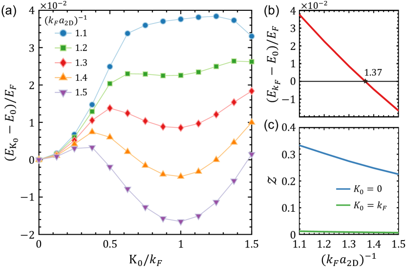
Figure 1: Polaron-to-molecule phase transition within the non-Gaussian variational states. (a) Polaron energy-momentum relation for various values of $(k_{F}a_{\mathrm{2D}})^{-1}$: as this parameter is increased, we observe that the minimum in the dispersion shifts from being located at $\mathrm{K}_{0}=0$ to $\mathrm{K}_{0}=k_{F}$, indicating a first-order polaron-to-molecule transition. Here $E_{F}=k_{F}^{2}/2m_{\mathrm{b}}$ is the Fermi energy. (b) This transition is predicted to occur at around $(k_{F}a_{\mathrm{2D}})^{-1}=1.37$. (c) The quasiparticle residue $\mathcal{Z}$ for $\mathrm{K}_{0}=0$ remains finite as the transition point is crossed; the residue for $\mathrm{K}_{0}=k_{F}$ is close to zero. Parameters used: $m_{\mathrm{imp}}=5m_{\mathrm{b}},k_{\Lambda}=5k_{F}$, and $\delta_{p}=2\pi/L=\left.k_{F}\right/8$.

In this section, we primarily investigate the polaron-to-molecule phase transition. We begin by exploring the full polaron energy-momentum relation, being interested in arbitrary total momentum $\mathbf{K}_{0}$. As such, the system is, in general, not rotationally symmetric, and numerical simulations are computationally expensive. To facilitate the computations, we consider, for now, rather heavy impurities, such as $m_{\mathrm{imp}}=5m_{\mathrm{b}}$, allowing us to choose a rather small UV cutoff $k_{\Lambda}$ because of relatively small binding energy $E_{B}$ – this energy decreases with increasing the ratio $m_{\mathrm{imp}}/m_{\mathrm{b}}$ [37]. If one is interested solely in the case with $\mathrm{K}_{0}=0$, the polaronic properties can be efficiently studied for arbitrary mass ratios using rotational symmetry, as we discuss below.

Figure 1(a) shows the polaron energy-momentum relation for various interaction strengths, as encoded in the dimensionless parameter $\left(k_{F}a_{\mathrm{2D}}\right)^{-1}$. We note that this dispersion $E_{\mathbf{K}_{0}}$ depends on $\mathrm{K}_{0}$ only (it does not depend on the direction of ${\mathbf{K}_{0}}$). Notably, for sufficiently strong interactions, the energy of the state at $\mathrm{K}_{0}=k_{F}$ becomes smaller than that at $\mathrm{K}_{0}=0$, indicating a change in the nature of the ground state – this change occurs at around $\left(k_{F}a_{\mathrm{2D}}\right)^{-1}=1.37$, as shown in Fig. 1(b). To better understand this transition, we now consider the quasiparticle residue defined as:

$$\mathcal{Z}=\left|\langle\mathrm{FS}|f_{\mathbf{K}_{0}}|\Psi_{\mathbf{K}_{0}}\rangle\right|^{2}.$$ (30)

This expression can be understood as the overlap between the non-interacting many-body state $f_{\mathbf{K}_{0}}^{\dagger}|\mathrm{FS}\rangle$ and the true ground state $|\Psi_{\mathbf{K}_{0}}\rangle$ with the impurity-bath interaction being switched on. Within the non-Gaussian states, the polaron residue is given by [20]:

$$\mathcal{Z}=\left|\langle\mathrm{FS}|\Psi_{\mathrm{GS}}\rangle\right|^{2}=\det\left(\mathrm{I}_{N}+2\Gamma_{\mathrm{FS}}\Gamma-\Gamma-\Gamma_{\mathrm{FS}}\right).$$ (31)

Figure 1(c) shows the quasiparticle residues at $\mathrm{K}_{0}=0$ and $\mathrm{K}_{0}=k_{F}$ across the transition: while the former smoothly decreases with $\left(k_{F}a_{\mathrm{2D}}\right)^{-1}$ and remains finite at the transition point, the latter is nearly zero. We remark that these results agree with the studies in Refs. [39, 40].

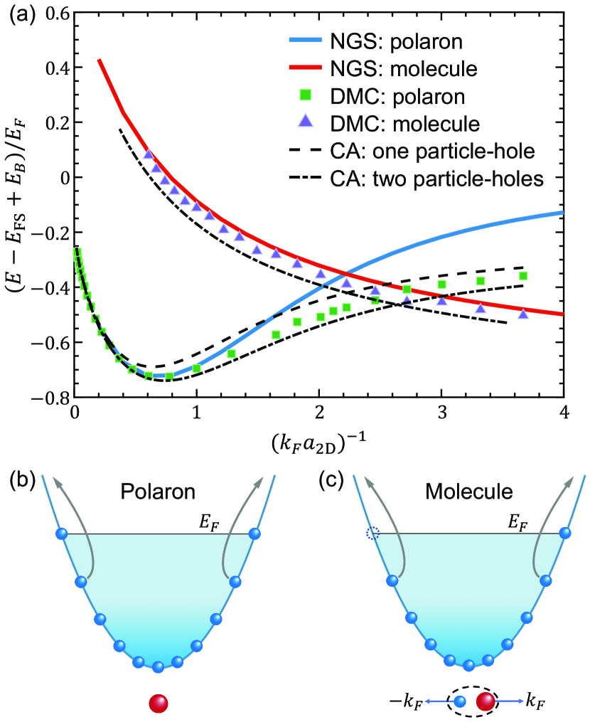
Figure 2: Comparison to the existing methods. (a) Energies of the polaronic and molecular states as a function of $\left(k_{F}a_{\mathrm{2D}}\right)^{-1}$ for the case of equal masses $m_{\mathrm{imp}}=m_{\mathrm{b}}$. The polaron-to-molecule transition point within the NGS approach is around $\left(k_{F}a_{\mathrm{2D}}\right)^{-1}=2.2$. For comparison, we also show the known results from DMC [66] and CA with one and two particle-hole excitations [38]. Here $E_{\mathrm{FS}}$ is the energy of the filled Fermi sea. Parameters used: $k_{\Lambda}=20k_{F}$, $\delta_{p}=k_{F}/40$, and $n_{\Lambda}=8$. (b) Schematic of the polaronic state $\mathbf{K}_{0}=(0,0)$: the impurity (red ball) has on average zero momentum and is coupled to particle-hole excitations (shown with arrows) of the Fermi sea (fermions are shown as blue balls). (c) Schematic of the molecular state $\mathbf{K}_{0}=(k_{F},0)$: the mobile impurity with momentum around $(k_{F},0)$ binds to the fermionic atom that has momentum $(-k_{F},0)$; the resulting molecule on average has zero momentum and weakly interacts with the rest of the Fermi sea.

These findings suggest the following physical picture. For weak and moderate interactions, the ground state is polaronic, it corresponds to the solution with $\mathrm{K}_{0}=0$, and it has finite quasiparticle weight [Fig. 2(b)]. For stronger interactions, the system exhibits a first-order phase transition into a molecular state, associated with the solution with $\mathrm{K}_{0}=k_{F}$ and vanishing quasiparticle residue $\mathcal{Z}=0$. In this regime, we find that for $\mathbf{K}_{0}=(k_{F},0)$, the fermion occupation at $(-k_{F},0)$ is essentially zero, indicating that this fermion has been removed from the Fermi sea to form a bound state with the impurity particle, so that the resulting molecule approximately has zero net momentum [Fig. 2(c)]. We finally remark that if one would have limited the analysis only to the $\mathrm{K}_{0}=0$ sector, instead of an abrupt transition, one would find a smooth crossover with gradual suppression of the quasiparticle weight.

When investigating the polaron-to-molecule transition for lighter impurities, such as $m_{\mathrm{imp}}=m_{\mathrm{b}}$, the binding energy $E_{B}$ becomes large, requiring a larger UV cutoff $k_{\Lambda}$ and making computations too expensive. We now argue that rotational symmetry can be naturally used to overcome this difficulty. The analysis of the polaronic state is immediately simplified because this state corresponds to $\mathbf{K}_{0}=(0,0)$, where the system is already rotationally invariant. For the molecular state, we have $\mathbf{K}_{0}=(k_{F},0)$ and, thus, rotational symmetry is broken. To restore this symmetry in our variational ansatz, we employ the following method: instead of working with $N_{f}$ fermions in the sector $\mathbf{K}_{0}=(k_{F},0)$, we add one more extra fermion and work in the sector $\mathbf{K}_{0}=(0,0)$. In other words, to describe the molecular state, from now on we will use the following variational wave function:

$$|\Psi_{\mathrm{NGS}}^{N_{f}+1}\rangle=U_{\mathrm{LLP}}f_{\mathbf{K}_{0}=0}^{\dagger}|\Psi_{\mathrm{GS}}^{N_{f}+1}\rangle,$$ (32)

where $|\Psi_{\mathrm{GS}}^{N_{f}+1}\rangle$ is chosen to be a Gaussian state for $N_{f}+1$ fermions. This insight comes from our previous observation that the impurity tends to bind one of the Fermi surface fermions – see Fig. 2(c). Thus, the newly introduced fermion fills the hole in the disturbed Fermi sea and makes the total momentum of the enlarged system zero. One can alternatively view the simplified molecular state in the spirit of Yosida’s ansatz [67], where one has a Fermi sea of $N_{f}$ fermions, and the impurity and extra bath fermion form a bound state with zero net momentum. In this molecule, both the impurity and extra fermion have to be outside the Fermi sea because their momenta should be opposite, but the extra fermion is excluded from the Fermi sea by the Pauli principle. We emphasize that our variational state goes beyond this simple ansatz because we take into account particle-hole excitations of the Fermi sea arising from the nonzero impurity-bath coupling.

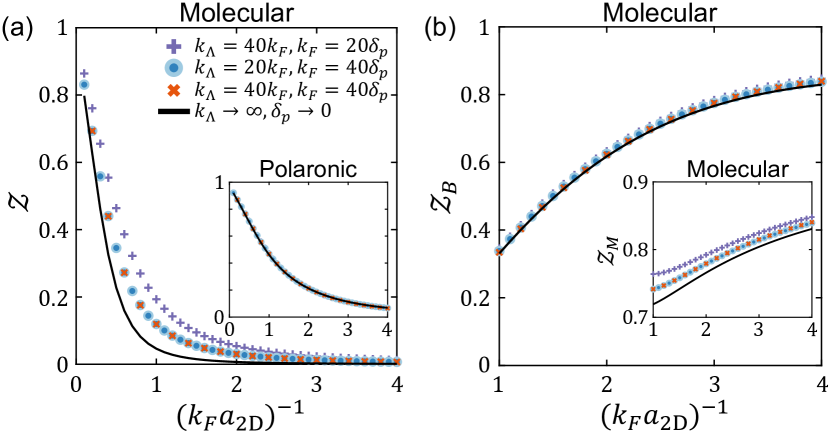
Figure 3: Various residues and their convergence with varying the UV cutoff $k_{\Lambda}$ and the linear system’s size encoded in $\delta_{p}$. Solid lines denote the extrapolation to the continuum limit $k_{\Lambda}\rightarrow\infty$ and $\delta_{p}\rightarrow 0$. Parameters are the same as in Fig. 2.

Figure 2(a) shows the energies of polaronic and molecular states as functions of $\left(k_{F}a_{\mathrm{2D}}\right)^{-1}$ for $m_{\mathrm{imp}}=m_{\mathrm{b}}$. We find that our non-Gaussian variational approach quantitatively agrees with the known results from the CA [38] and DMC calculations [66]. Our method is particularly accurate at capturing the molecular branch, confirming the validity of the simplified molecular ansatz $|\Psi_{\mathrm{NGS}}^{N_{f}+1}\rangle$. The polaron-to-molecule transition is predicted to occur around $\left(k_{F}a_{\mathrm{2D}}\right)^{-1}=2.2$. Across the transition point, the polaronic residue $\mathcal{Z}$ remains finite [inset of Fig. 3(a)], but the molecular one is essentially zero [Fig. 3(a)]. Accurate analysis of the convergence of our results with the UV cutoff $k_{\Lambda}$ and the parameter $\delta_{p}$ that encodes the linear system’s size indicates that indeed, in the limit $k_{\Lambda}\rightarrow\infty$ and $\delta_{p}\rightarrow 0$, the molecular residue approaches zero for $\left(k_{F}a_{\mathrm{2D}}\right)^{-1}\gtrsim 2.2$ – see the solid line in Fig. 3(a). For $\left(k_{F}a_{\mathrm{2D}}\right)^{-1}<2.2$, the ground state is polaronic, and, as such, the molecular state corresponds to some excited state. Since the size of this molecule becomes more extensive as $\left(k_{F}a_{\mathrm{2D}}\right)^{-1}$ is decreased, accurate computation of the residue $\mathcal{Z}$ for small $\left(k_{F}a_{\mathrm{2D}}\right)^{-1}$ requires a smaller infrared cutoff $\delta_{p}$.

Finally, we finish this section by introducing two more “molecular residues” that help characterize the molecular state better. Since the quasiparticle residue is close to being one in the polaronic phase and vanishes in the molecular phase, the new molecular residues should display the opposite behavior. Motivated by this, we introduce the first one as $\mathcal{Z}_{M}=|\langle\Psi_{M}|\Psi_{\mathrm{NGS}}^{N_{f}+1}\rangle|^{2}$, where $|\Psi_{M}\rangle=\sum_{\left|\mathbf{k}\right|>k_{F}}\varphi_{\mathbf{k}}^{M}c_{\mathbf{k}}^{\dagger}f_{-\mathbf{k}}^{\dagger}\left|\mathrm{FS}\right\rangle$ encodes the Yosida ansatz. Optimization of the variational parameters gives $\varphi_{\mathbf{k}}^{M}\propto-1/(k^{2}+a_{\mathrm{2D}}^{-2}-k_{F}^{2})$. We define the second residue as $\mathcal{Z}_{B}=|\langle\Psi_{B}|\Psi_{\mathrm{NGS}}^{N_{f}+1}\rangle|^{2}$, where $|\Psi_{B}\rangle=\sum_{\left|\mathbf{k}\right|>k_{F}}\varphi_{\mathbf{k}}^{B}c_{\mathbf{k}}^{\dagger}f_{-\mathbf{k}}^{\dagger}\left|\mathrm{FS}\right\rangle$ with the parameters $\varphi_{\mathbf{k}}^{B}$ given by:

$$\varphi_{\mathbf{k}}^{B}=\frac{1}{L\sqrt{\mathcal{N}}}\frac{1}{-1/(2m_{\mathrm{r}}a_{X}^{2})-\varepsilon_{\mathrm{imp},\mathbf{k}}-\varepsilon_{\mathrm{b},\mathbf{k}}},$$ (33)

Here, $\mathcal{N}=m_{\mathrm{r}}^{2}a_{X}^{2}/[\pi(1+k_{F}^{2}a_{X}^{2})]$ is a normalization constant. The residue $\mathcal{Z}_{B}$ is useful because it can be measured with ultracold atom experiments, as we elaborate in the next section. We also postpone the discussion of the newly introduced length $a_{X}$ to the next section but will assume here that it is much smaller than the Fermi wavelength. We only emphasize here that $a_{X}$ is different from the scattering length $a_{\mathrm{2D}}$.

We observe that the states $|\Psi_{B,M}\rangle$ can be written as $|\Psi_{B,M}\rangle=U_{\mathrm{LLP}}f_{\mathbf{0}}^{\dagger}|0\rangle_{\mathrm{imp}}\otimes|\bar{\Psi}_{B,M}\rangle$, with the Gaussian states $|\bar{\Psi}_{B,M}\rangle$ given by:

$$|\bar{\Psi}_{B,M}\rangle=\sum_{\left|\mathbf{k}\right|>k_{F}}\varphi^{B,M}_{\mathbf{k}}c_{\mathbf{k}}^{\dagger}\left|\mathrm{FS}\right\rangle.$$ (34)

The molecular residues $\mathcal{Z}_{B,M}$ are then computed through the corresponding covariance matrices $\Gamma_{B,M}$ as:

$$\mathcal{Z}_{B,M} =\left|\langle\bar{\Psi}_{B,M}|\Psi_{\mathrm{GS}}\rangle\right|^{2}$$

$$=\det\left(\,\mathrm{I}_{N}+2\Gamma_{B,M}\Gamma-\Gamma-\Gamma_{B,M}\right).$$ (35)

Figure 3(b) shows the dependence of the two residues on $(k_{F}a_{\mathrm{2D}})^{-1}$. Both of them approach one in the molecular phase. Physically, deep inside the molecular phase, the impurity and one bath fermion form a tight bare bound state, that in turn creates a scattering potential to the rest of the bath particles. Close to the phase transition, the bath fermions start to strongly affect the structure of the bound state, resulting in, for instance, a small overlap $|\langle\Psi_{B}|\Psi_{\mathrm{NGS}}^{N_{f}+1}\rangle|$. For the residue $\mathcal{Z}_{M}$, we find that even though the parameters $\varphi_{\mathbf{k}}^{M}$ are being optimized, $\mathcal{Z}_{M}\sim 0.8$ is still smaller than one in the molecular phase. We attribute this deviation to the fact that the Yosida ansatz, in contrast to the non-Gaussian wave function, does not take into account the backreaction from the Fermi sea on the formation of the molecular bound state.

IV Dynamical properties

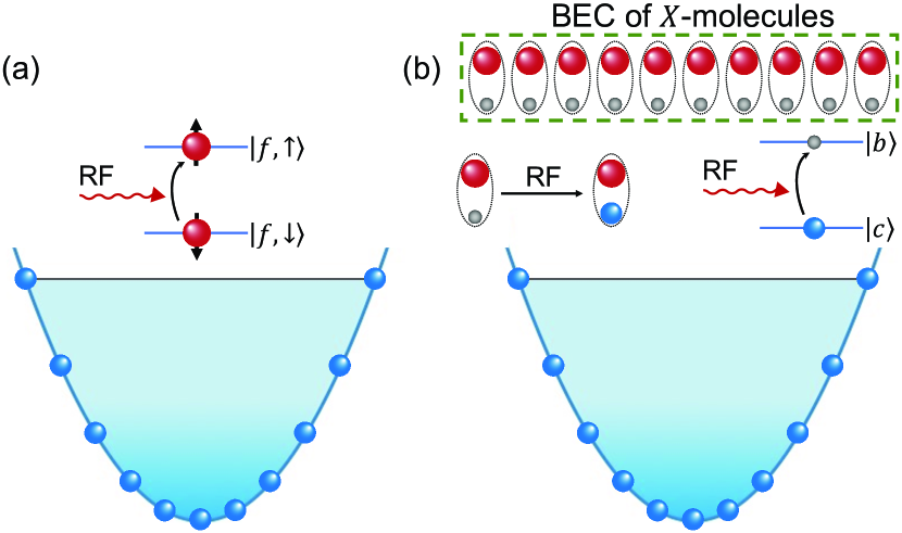
Figure 4: Possible cold-atom setups. In the platform of panel (a), we assume that the impurity atom (red ball) has two hyperfine states $\ket{f,\uparrow}$ and $\ket{f,\downarrow}$. Initially, the impurity is prepared in $\ket{f,\downarrow}$, which is not interacting with the fermionic bath (represented with blue balls). By applying a weak RF-pulse, one drives a transition into $\ket{f,\uparrow}$, which interacts strongly with the Fermi sea. This protocol gives access to the polaronic spectral properties. The setup of panel (b) is different. Here we consider the initial state to be a Fermi sea of $c$-fermions and a BEC of $X$-molecules that are composed of atoms $f$ and $b$ (grey balls). Now, we assume that $\ket{c}$ and $\ket{b}$ are two hyperfine states, which are then coupled by a weak RF-pulse. Such an RF pulse breaks a “grey-red” $X$-molecule and leaves behind one strongly interacting “red” $f$-fermion and an additional “blue” majority $c$-fermion. These “red” and additional “blue” fermions are created as a pair with a wave function set by the wave function of the original $X$-molecule. As such, this protocol gives access to the molecular spectral properties.

Having established the reliability of the non-Gaussian approach to the ground-state properties of 2D Fermi polaron, we move on to discuss dynamics. We remark that accurate analysis of out-of-equilibrium properties represents one of the main advantages of our method compared to, for instance, DMC. Here, we first discuss possible cold-atom experiments that enable one to measure polaronic and molecular spectral functions, in particular, to probe the residues $\mathcal{Z}$ and $\mathcal{Z}_{B}$. We then analyze these polaronic and molecular spectral properties separately in the following subsections.

IV.1 Cold-atom platforms

We begin by discussing the conventional experimental protocol for measuring polaronic spectral properties [Fig. 4(a)]. We will assume that the impurity atom has two hyperfine states, one of which $\ket{f,\downarrow}$ is not coupled to the $c$-fermions, while the other $\ket{f,\uparrow}$ strongly interacts with the bath. The system is initially prepared in $\ket{f,\downarrow}\otimes\ket{\rm FS}$, which is then driven into $|\Psi_{0}\rangle=\ket{f,\uparrow}\otimes\ket{\rm FS}$ by a weak RF-pulse. Then, Ramsey interferometry enables one to probe the dynamical overlap function $S(t)=e^{iE_{\mathrm{FS}}t}\langle\Psi_{0}|\exp(-iHt)|\Psi_{0}\rangle$, where $E_{\mathrm{FS}}$ is the total energy of the Fermi sea. The impurity spectral function $\mathcal{A}(\omega)$, also accessible with RF-spectroscopy, is given by:

$$\mathcal{A}(\omega)=\frac{1}{\pi}\mathrm{Re}\int_{0}^{\infty}dt\,e^{i\omega t}\,S(t).$$ (36)

We remark that while we discuss here the setup to probe correlations when the total momentum is zero $\mathbf{K}_{0}=\mathbf{0}$, it can be extended to explore $\mathbf{K}_{0}\neq\mathbf{0}$ (see Ref. [20] for a related discussion).

The protocol to measure molecular properties is different [Fig. 4(b)]. We now choose the initial state to be a Fermi sea of $c$-atoms and a BEC of $X$-molecules, composed of $\ket{f}$ and $\ket{b}$ atoms. In contrast to the previous setup, here $\ket{b}$ and $\ket{c}$ are assumed to be two hyperfine states. As we demonstrate in Appendix A by performing adiabatic elimination of $b$-fermions, a weak RF-pulse is then described via:

$$H_{\mathrm{RF}}=\frac{\Omega_{\mathrm{RF}}}{L}\sum_{|\mathbf{k}|\lesssim a_{X}^{-1}}\frac{e^{-i\omega t}}{E_{X}-\varepsilon_{\mathrm{imp},\mathbf{k}}-\varepsilon_{\mathrm{b},\mathbf{k}}}c_{\mathbf{k}}^{\dagger}f_{-\mathbf{k}}^{\dagger}+\mathrm{H.c.}$$ (37)

Here $E_{X}=-1/(2m_{\mathrm{r}}a_{X}^{2})$ is the binding energy of an $X$-molecule; $a_{X}$ is the corresponding scattering length assumed to be much smaller than the Fermi wavelength $a_{X}k_{F}\ll 1$. The effective coupling $\Omega_{\mathrm{RF}}$ is proportional to $\sqrt{N_{X}}$ and the intensity of the pulse, with $N_{X}$ being the total number of $X$-molecules. One can view such an RF-pulse as if it substitutes a $b$-atom in a tightly-bound $X$-molecule with a $c$-atom. The corresponding dynamical overlap is given by: $S_{B}(t)=e^{i(E_{\mathrm{FS}}+E_{F})t}\langle\Psi_{B}|\exp(-iHt)|\Psi_{B}\rangle$, where the state $|\Psi_{B}\rangle$ has been defined in the previous section, cf. Eq. (33). The molecular spectral function $\mathcal{A}_{B}(\omega)$ is then defined as:

$$\mathcal{A}_{B}(\omega)=\frac{1}{\pi}\text{Re}\int_{0}^{\infty}dt\,e^{i\omega t}\,S_{B}(t).$$ (38)

Having introduced all the relevant dynamical quantities, we turn to explore them in the next subsections.

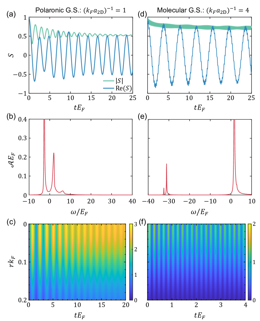
Figure 5: Polaronic spectral properties. Left and right panels correspond to the cases with the ground state being polaronic $(k_{F}a_{\mathrm{2D}})^{-1}=1$ and with it being molecular $(k_{F}a_{\mathrm{2D}})^{-1}=4$, respectively. Panels (c) and (f) display the evolution of the real-space density $\mathbf{\delta}\rho(r,t)=\rho(r,t)-\rho(r,0)$ (this quantity has the unit of $k_{F}^{2}$). Parameters used: $m_{\mathrm{imp}}=m_{\mathrm{b}}$, $k_{\Lambda}=20k_{F}$, $\delta_{p}=\left.k_{F}\right/40$, and $n_{\Lambda}=8$.

IV.2 Polaronic spectral properties

In the co-moving LLP frame, the dynamical overlap reads: $S(t)=\langle\mathrm{FS}|\bar{\Psi}_{\boldsymbol{0}}(t)\rangle$, where $|\bar{\Psi}_{\boldsymbol{0}}(t)\rangle=\exp(-iH_{\mathrm{LLP}}t)|\mathrm{FS}\rangle$ – this latter state is obtained via the real-time equations of motion detailed in Sec. II. Within the non-Gaussian states, $S(t)$ is computed through $\theta$ and $U$ as:

$$S(t)=e^{-i(\theta(t)-E_{\mathrm{FS}}t)}\det\left\{\mathrm{I}_{N}-[\mathrm{I}_{N}-U(t)]\Gamma_{\mathrm{FS}}^{\mathrm{T}}\right\}.$$ (39)

We begin by considering $(k_{F}a_{\mathrm{2D}})^{-1}=1$, in which case the ground state is polaronic. Figure 5(a) shows the dynamics of Re$\,S(t)$ and $|S(t)|$ that display damped oscillatory behavior. At long times, $|S(t)|$ approaches a finite value, which is nothing but the quasiparticle residue $\mathcal{Z}$. The spectral function $\mathcal{A}(\omega)$ is shown in Fig. 5(b). We find that the ground-state energy, as determined by the position of the sharp peak in $\mathcal{A}(\omega)$ (attractive polaron), and the corresponding oscillator strength are in agreement with the energy and quasiparticle residue calculations in Figs. 2 and 3. The additional hump in $\mathcal{A}(\omega)$ for $\omega>0$ (repulsive polaron) occurs due to the fact that the initial state has a finite overlap with the continuum of particle-hole excitations – the position and width of this hump determine the frequency and decay rate of $|S(t)|$ at initial times. Figure 5(c) shows the dynamics of the real-space fermionic density. Upon the abrupt creation of the impurity at $t=0$, the density near the impurity initially exhibits profound oscillations but then reaches a steady state at longer times.

We turn to consider the case with $(k_{F}a_{\mathrm{2D}})^{-1}=4$, characterized by the ground state being molecular. To properly account for the finite-momentum nature of the molecular state, here we follow the previous section and consider $N_{f}$ + 1 fermions. Figure 5(e) shows the spectral function $\mathcal{A}(\omega)$, which displays two sharp peaks at $\omega\sim 1.57E_{F}$ and $\omega\sim-31.1E_{F}$ corresponding to the energies of the repulsive and attractive polarons, respectively, in agreement with the results of Ref. [56]. There is an additional tiny peak at $\omega\sim-32.5E_{F}$, which emerges due to the finite size effects and vanishes in the thermodynamic limit. As we discuss in the following subsection, this tiny peak corresponds to the energy of the molecular state. The time-dependent overlap function $S(t)$ exhibits long-lived oscillations shown in Fig. 5(d), which can be understood as arising from quantum beatings between the attractive and repulsive polarons. We note that the initial state $|\Psi_{0}(t=0)\rangle=|\mathrm{FS}\rangle$ has finite overlaps with both of these polaron branches. As $|\Psi_{0}(t)\rangle$ propagates in time, parts of the wave function corresponding to the two polarons evolve with different energies, and since the system seems to never relax to the molecular ground state locally [Fig. 5(d)], it results in long-lived oscillations of the fermionic density near the impurity, as illustrated in Fig. 5(f).

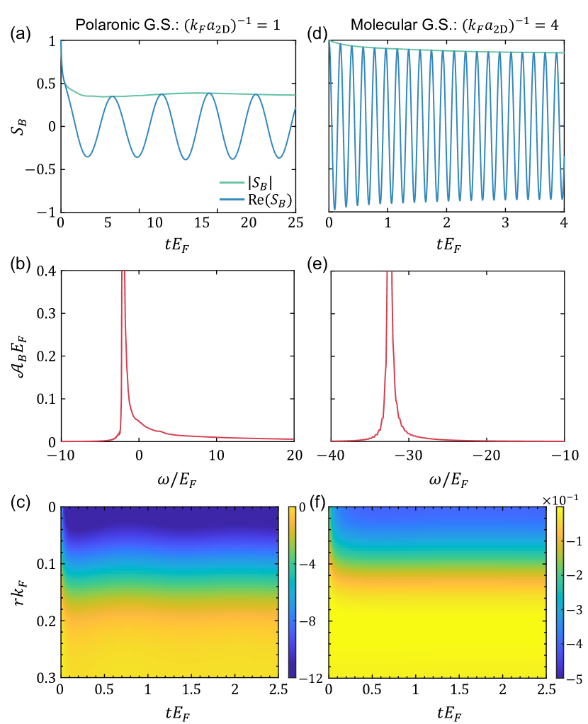
Figure 6: The same as in Fig. 5, except here we show molecular spectral properties. Here we fix $(k_{F}a_{X})^{-1}=4$.

IV.3 Molecular spectral properties

Here we do a similar analysis as in the preceding subsection, but now consider the experimental protocol in Fig. 4(b) that enables one to probe molecular spectral properties. In the numerical simulations, we consider the initial state $|\Psi_{B}(t=0)\rangle=\sum_{\left|\mathbf{k}\right|>k_{F}}\varphi_{\mathbf{k}}^{B}c_{\mathbf{k}}^{\dagger}f_{-\mathbf{k}}^{\dagger}\left|\mathrm{FS}\right\rangle$ in the lab frame, which describes a deeply bound molecule created on top of the Fermi sea. The corresponding dynamical overlap function in the co-moving frame becomes: $S_{B}(t)=$ $\langle\bar{\Psi}_{B}(t=0)|\bar{\Psi}_{B}(t)\rangle$, where $|\bar{\Psi}_{B}(t)\rangle=\exp(-iH_{\mathrm{LLP}}t)|\bar{\Psi}_{B}(t=0)\rangle$, and $|\bar{\Psi}_{B}(t=0)\rangle=\sum_{\left|\mathbf{k}\right|>k_{F}}\varphi_{\mathbf{k}}^{B}c_{\mathbf{k}}^{\dagger}\left|\mathrm{FS}\right\rangle$ is the initial molecule state in the LLP frame, i.e., Eq. (34). Hereafter, for concreteness, we focus on the case $(k_{F}a_{X})^{-1}=4$. The dynamical overlap function $S_{B}(t)$ is calculated analytically:

$$S_{B}(t)=e^{-i(\theta(t)-(E_{\mathrm{FS}}+E_{F})t)}\det\left\{\mathrm{I}_{N}-[\mathrm{I}_{N}-U(t)]\Gamma_{B}^{\mathrm{T}}\right\}.$$ (40)

Implicit in the discussion below is that the bath is composed of $N_{f}+1$ fermions.

We first discuss the polaronic regime $(k_{F}a_{\mathrm{2D}})^{-1}=1$ – the results of our simulations are summarized in Fig. 6 (left panels). We find that the frequency of the sharp peak in the molecular spectral function $\mathcal{A}_{B}(\omega)$ [Fig. 6(b)] is $\omega\sim-2.07E_{F}$, in good agreement with the ground-state energy $E_{\mathrm{GS}}\sim-2.09E_{F}$ of $N_{f}+1$ fermions in the total momentum sector $\mathbf{K}_{0}=\mathbf{0}$. Our results suggest that the initial tight bound state $|\bar{\Psi}_{B}(t=0)\rangle$ has a finite overlap $\sim 0.3$ with the ground state – this is indicated by the steady-state value of $|S_{B}(t)|$ [Fig. 6(a)]. The long tail in $\mathcal{A}_{B}(\omega)$ also implies that the state $|\bar{\Psi}_{B}(t=0)\rangle$ has a substantial spectral weight associated with the continuum of particle-hole excitations of the Fermi sea.

Deep in the molecular phase, $(k_{F}a_{\mathrm{2D}})^{-1}=4$ [right panels in Fig. 6], the initial two-body bound state on top of the the undisturbed Fermi sea quickly relaxes to the true molecular ground state. The sharp peak in the spectral function $\mathcal{A}_{B}(\omega)$ [Fig. 6(e)] is at $\omega\sim-32.5E_{F}$, which is exactly the molecular ground-state energy. At long times, $|S_{B}(t)|\sim 0.8$ [Fig. 6(d)] – this value agrees with the analysis in Fig. 3(b) of the molecular residues.

Finally, in both regimes, we find that the density profiles [Fig. 6(c) and 6(f)] show rapid relaxational dynamics.

V Summary and outlook

In this paper, we analyzed both the ground-state and dynamical properties of Fermi polarons in two spatial dimensions using a new family of non-Gaussian variational wave functions. We showed that this class of states captures the polaron-to-molecule transition that emerges as one increases the attractive interaction strength. Energies of both polaronic and molecular states, as well as the transition point, are in good agreement with the known Monte-Carlo simulations. Our theory, in contrast to conventional numerical methods, enables efficient computation of the polaronic spectral functions, accessible with RF spectroscopy. In addition to the commonly discussed quasiparticle spectral function and residue, we introduced molecular spectral function and residue that help characterize better the nature of the molecular state. We discussed how these molecular properties could be measured with RF-like experiments, where we proposed the initial state to contain a BEC of tightly-bound molecules.

While the analysis in our paper focused on systems of ultracold atoms, we expect that our results will be relevant for exciton-electron mixtures in TMD materials. In particular, we anticipate that the proposed experimental protocol for the molecular spectral properties can be realized in bilayer TMDs. Indeed, interlayer excitons are relatively long-lived and can be used to achieve BEC states. Terahertz pulses can then be used to convert these interlayer excitons into intralayer ones, demonstrate the existence of Feshbach resonances, and probe the molecular spectral function [44, 68].

Appendix A Effective RF-Hamiltonian for the molecular spectral function

Following the setup in Fig. 4(b) of the main text, here we derive an effective Hamiltonian that describes the corresponding RF-pulse. In the rotating frame, the system’s Hamiltonian is given by $H=H_{0}+V$, where

$$H_{0}= \sum_{\mathbf{k}}\left[\left(\varepsilon_{\mathrm{{b},\mathbf{k}}}-\omega-\Delta\right)c_{\mathbf{k}}^{\dagger}c_{\mathbf{k}}+\tilde{\varepsilon}_{\mathbf{k}}b_{\mathbf{k}}^{\dagger}b_{\mathbf{k}}+\varepsilon_{\mathrm{{imp},\mathbf{k}}}f_{\mathbf{k}}^{\dagger}f_{\mathbf{k}}\right]$$

$$+E_{X}X_{\mathbf{0}}^{\dagger}X_{\mathbf{0}},$$ (41)

and

$$V= \sum_{\mathbf{k}}\left(g_{\mathbf{k}}X_{\mathbf{0}}f_{-\mathbf{k}}^{\dagger}b_{\mathbf{k}}^{\dagger}+\text{H.c.}\right)+\lambda\sum_{\mathbf{k}}\left(c_{\mathbf{k}}^{\dagger}b_{\mathbf{k}}+\text{H.c.}\right).$$ (42)

Here $\omega$ is the frequency of the RF-pulse, $b_{\mathbf{k}}$ ($b_{\mathbf{k}}^{\dagger}$) is the annihilation (creation) operator of the fermion $b$ with momentum $\mathbf{k}$ and dispersion $\tilde{\varepsilon}_{\mathbf{k}}=\varepsilon_{\mathrm{{b},\mathbf{k}}}$, and $\Delta$ is the energy difference between the states $b$ and $c$. For the BEC of $X$-molecules, we consider the mode $X_{\mathbf{0}}$ with zero total momentum $\mathbf{{k}={0}}$ only; it has binding energy $E_{X}$. The first term in Eq. (42) describes that an $X$-molecule can recombine into a pair of atoms $f$ and $b$ with the transition amplitude $g_{\mathbf{k}}$, and vice versa. The second term in Eq. (42) encodes the RF-pulse that couples the states $\ket{b}$ and $\ket{c}$.

We now use the Schrieffer-Wolf transformation [69] to eliminate $V$ and obtain the effective Hamiltonian $H^{\prime}=H_{0}+[V,S]/2$, where the generating operator

$$S= -\sum_{\mathbf{k}}\frac{1}{\varepsilon_{\mathrm{imp},\mathbf{k}}+\tilde{\varepsilon}_{\mathbf{k}}-E_{X}}\left(g_{\mathbf{k}}X_{\mathbf{0}}f_{-\mathbf{k}}^{\dagger}b_{\mathbf{k}}^{\dagger}-\text{H.c.}\right)$$

$$-\sum_{\mathbf{k}}\frac{\lambda}{\varepsilon_{\mathrm{b},\mathbf{k}}-\tilde{\varepsilon}_{\mathbf{k}}-\omega-\Delta}\left(c_{\mathbf{k}}^{\dagger}b_{\mathbf{k}}-\text{H.c.}\right)$$ (43)

satisfies $[H_{0},S]+V=0$. In the explicit form, the effective interaction $V_{\mathrm{eff}}=H^{\prime}-H_{0}$ reads

$$V_{\mathrm{eff}}= \frac{1}{2}\sum_{\mathbf{k}}\frac{\lambda\left\langle X_{\mathbf{0}}\right\rangle}{\varepsilon_{\mathrm{{imp},\mathbf{k}}}+\tilde{\varepsilon}_{\mathbf{k}}-E_{X}}\left(g_{\mathbf{k}}c_{\mathbf{k}}^{\dagger}f_{-\mathbf{k}}^{\dagger}+\text{H.c.}\right)$$

$$+\frac{1}{2}\sum_{\mathbf{k}}\frac{\lambda\left\langle X_{\mathbf{0}}\right\rangle}{\varepsilon_{\mathrm{b},\mathbf{k}}-\tilde{\varepsilon}_{\mathbf{k}}-\omega-\Delta}\left(g_{\mathbf{k}}c_{\mathbf{k}}^{\dagger}f_{-\mathbf{k}}^{\dagger}+\text{ H.c.}\right)$$

$$+\sum_{\mathbf{k}}\frac{|g_{\mathbf{k}}|^{2}\left\langle X_{\mathbf{0}}\right\rangle^{2}}{\varepsilon_{\mathrm{{imp},\mathbf{k}}}+\tilde{\varepsilon}_{\mathbf{k}}-E_{X}}\left(f_{-\mathbf{k}}^{\dagger}f_{-\mathbf{k}}+b_{\mathbf{k}}^{\dagger}b_{\mathbf{k}}-1\right)$$

$$+\sum_{\mathbf{k}}\frac{\lambda^{2}}{\varepsilon_{\mathrm{b},\mathbf{k}}-\tilde{\varepsilon}_{\mathbf{k}}-\omega-\Delta}\left(c_{\mathbf{k}}^{\dagger}c_{\mathbf{k}}-b_{\mathbf{k}}^{\dagger}b_{\mathbf{k}}\right),$$ (44)

where the operator $X_{\mathbf{0}}$ is replaced by its expectation value $\left\langle X_{\mathbf{0}}\right\rangle$ set by the BEC of $X$-molecules. Among the four terms appearing in Eq. (44), the last two are unimportant as they give small modifications to the dispersion relations. The second term is expected to be negligible, if one assumes $|\Delta|\gg|\omega|,|E_{X}|$, while the first one describes the RF-perturbation. In the original frame, this latter contribution becomes:

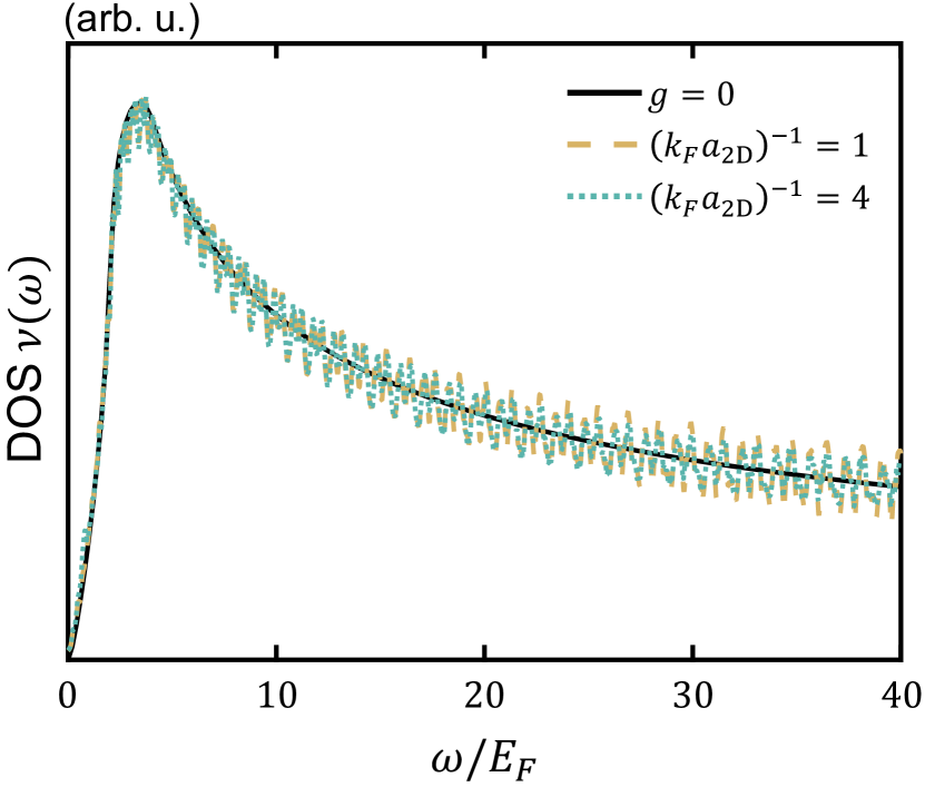
Figure 7: Density of states $\nu(\omega)$ (DOS) of collective modes for various interaction strengths. Parameters used: $\mathrm{K}_{0}=0$, $k_{F}=10\delta_{p}$, $k_{\Lambda}=10k_{F}$, and $n_{\Lambda}=10$.

$$H_{\mathrm{RF}}=\frac{1}{2}\sum_{\mathbf{k}}\frac{\lambda\left\langle X_{\mathbf{0}}\right\rangle}{\varepsilon_{\mathrm{{imp},\mathbf{k}}}+\tilde{\varepsilon}_{\mathbf{k}}-E_{X}}\left(e^{-i\omega t}g_{\mathbf{k}}c_{\mathbf{k}}^{\dagger}f_{-\mathbf{k}}^{\dagger}+\text{ H.c.}\right).$$ (45)

The transition amplitude $g_{\mathbf{k}}$ can be approximated as a constant, provided that it varies slowly in the range $|\mathbf{k}|\lesssim a_{X}^{-1}$.

Appendix B DOS of collective modes

Collective modes in the 1D Fermi polaron proved particularly important because they help understand not only equilibrium but also far-from-equilibrium phenomena, such as the quantum flutter [20]. Motivated by this and following Sec. II.4, here we compute the density of states (DOS) $\nu(\omega)=\sum_{n}\delta(\omega-\omega_{n})$ of collective modes in the 2D polaron problem ($\omega_{n}$ labels energies of the excitations). Figure 7 shows the result of such an analysis.

We do not find any particular features in $\nu(\omega)$, such as a sharp peak that could resemble the quantum flutter. What is surprising is that DOSs for notably different interaction strengths look similar, which could be because we restrict our analysis to the momentum sector $\mathbf{K}_{0}=\mathbf{0}$. It could also be that far-from-equilibrium dynamics in the 2D Fermi polaron are very different from the 1D case. We leave the analysis for generic total momenta $\mathbf{K}_{0}\neq\mathbf{0}$ to future work.

References

- Anderson [1967] P. W. Anderson, Phys. Rev. Lett. 18, 1049 (1967).
- Ohtaka and Tanabe [1990] K. Ohtaka and Y. Tanabe, Rev. Mod. Phys. 62, 929 (1990).
- Mahan [2000] G. D. Mahan, Many-Particle Physics (Springer US, Boston, MA, 2000).
- Anderson and Yuval [1969] P. W. Anderson and G. Yuval, Phys. Rev. Lett. 23, 89 (1969).
- Yuval and Anderson [1970] G. Yuval and P. W. Anderson, Phys. Rev. B 1, 1522 (1970).
- Tanabe and Ohtaka [1985] Y. Tanabe and K. Ohtaka, Phys. Rev. B 32, 2036 (1985).
- Hentschel et al. [2005] M. Hentschel, D. Ullmo, and H. U. Baranger, Phys. Rev. B 72, 035310 (2005).
- Nazarov and Blanter [2009] Y. V. Nazarov and Y. M. Blanter, Quantum Transport: Introduction to Nanoscience (Cambridge University Press, Cambridge, 2009).
- Schirotzek et al. [2009] A. Schirotzek, C.-H. Wu, A. Sommer, and M. W. Zwierlein, Phys. Rev. Lett. 102, 230402 (2009).
- Zhang et al. [2012] Y. Zhang, W. Ong, I. Arakelyan, and J. E. Thomas, Phys. Rev. Lett. 108, 235302 (2012).
- Schmidt et al. [2016] R. Schmidt, H. R. Sadeghpour, and E. Demler, Phys. Rev. Lett. 116, 105302 (2016).
- Ashida et al. [2019] Y. Ashida, T. Shi, R. Schmidt, H. R. Sadeghpour, J. I. Cirac, and E. Demler, Phys. Rev. Lett. 123, 183001 (2019).
- Sarachik et al. [1964] M. P. Sarachik, E. Corenzwit, and L. D. Longinotti, Phys. Rev. 135, A1041 (1964).
- Hewson [1993] A. C. Hewson, The Kondo Problem to Heavy Fermions, Cambridge Studies in Magnetism (Cambridge University Press, Cambridge, 1993).
- Gegenwart et al. [2008] P. Gegenwart, Q. Si, and F. Steglich, Nature Phys 4, 186 (2008).
- Kirchner et al. [2020] S. Kirchner, S. Paschen, Q. Chen, S. Wirth, D. Feng, J. D. Thompson, and Q. Si, Rev. Mod. Phys. 92, 011002 (2020).
- Storchak and Prokof’ev [1998] V. G. Storchak and N. V. Prokof’ev, Rev. Mod. Phys. 70, 929 (1998).
- Rosch [1999] A. Rosch, Advances in Physics 48, 295 (1999).
- Castella and Zotos [1993] H. Castella and X. Zotos, Phys. Rev. B 47, 16186 (1993).
- Dolgirev et al. [2021] P. E. Dolgirev, Y.-F. Qu, M. B. Zvonarev, T. Shi, and E. Demler, Phys. Rev. X 11, 041015 (2021).
- Astrakharchik and Pitaevskii [2004] G. E. Astrakharchik and L. P. Pitaevskii, Phys. Rev. A 70, 013608 (2004).
- Cherny et al. [2012] A. Y. Cherny, J.-S. Caux, and J. Brand, Front. Phys. 7, 54 (2012).
- Schmidt and Enss [2011] R. Schmidt and T. Enss, Phys. Rev. A 83, 063620 (2011).
- Kohstall et al. [2012] C. Kohstall, M. Zaccanti, M. Jag, A. Trenkwalder, P. Massignan, G. M. Bruun, F. Schreck, and R. Grimm, Nature 485, 615 (2012).
- Koschorreck et al. [2012] M. Koschorreck, D. Pertot, E. Vogt, B. Fröhlich, M. Feld, and M. Köhl, Nature 485, 619 (2012).
- Cetina et al. [2016] M. Cetina, M. Jag, R. S. Lous, I. Fritsche, J. T. M. Walraven, R. Grimm, J. Levinsen, M. M. Parish, R. Schmidt, M. Knap, and E. Demler, Science 354, 96 (2016).
- Scazza et al. [2017] F. Scazza, G. Valtolina, P. Massignan, A. Recati, A. Amico, A. Burchianti, C. Fort, M. Inguscio, M. Zaccanti, and G. Roati, Phys. Rev. Lett. 118, 083602 (2017).
- Yan et al. [2019] Z. Yan, P. B. Patel, B. Mukherjee, R. J. Fletcher, J. Struck, and M. W. Zwierlein, Phys. Rev. Lett. 122, 093401 (2019).
- Ness et al. [2020] G. Ness, C. Shkedrov, Y. Florshaim, O. K. Diessel, J. von Milczewski, R. Schmidt, and Y. Sagi, Phys. Rev. X 10, 041019 (2020).
- Chin et al. [2010] C. Chin, R. Grimm, P. Julienne, and E. Tiesinga, Rev. Mod. Phys. 82, 1225 (2010).
- Prokof’ev and Svistunov [2008a] N. Prokof’ev and B. Svistunov, Phys. Rev. B 77, 020408 (2008a).
- Prokof’ev and Svistunov [2008b] N. V. Prokof’ev and B. V. Svistunov, Phys. Rev. B 77, 125101 (2008b).
- Chevy [2006] F. Chevy, Phys. Rev. A 74, 063628 (2006).
- Combescot et al. [2007] R. Combescot, A. Recati, C. Lobo, and F. Chevy, Phys. Rev. Lett. 98, 180402 (2007).
- Combescot and Giraud [2008] R. Combescot and S. Giraud, Phys. Rev. Lett. 101, 050404 (2008).
- Zöllner et al. [2011] S. Zöllner, G. M. Bruun, and C. J. Pethick, Phys. Rev. A 83, 021603 (2011).
- Parish [2011] M. M. Parish, Phys. Rev. A 83, 051603 (2011).
- Parish and Levinsen [2013] M. M. Parish and J. Levinsen, Phys. Rev. A 87, 033616 (2013).
- Cui [2020] X. Cui, Phys. Rev. A 102, 061301 (2020).
- Peng et al. [2021] C. Peng, R. Liu, W. Zhang, and X. Cui, Phys. Rev. A 103, 063312 (2021).
- Sidler et al. [2017] M. Sidler, P. Back, O. Cotlet, A. Srivastava, T. Fink, M. Kroner, E. Demler, and A. Imamoglu, Nature Phys 13, 255 (2017).
- Efimkin and MacDonald [2017] D. K. Efimkin and A. H. MacDonald, Phys. Rev. B 95, 035417 (2017).
- Fey et al. [2020] C. Fey, P. Schmelcher, A. Imamoglu, and R. Schmidt, Phys. Rev. B 101, 195417 (2020).
- Kuhlenkamp et al. [2022] C. Kuhlenkamp, M. Knap, M. Wagner, R. Schmidt, and A. Imamoğğlu, Phys. Rev. Lett. 129, 037401 (2022).
- Shi et al. [2018] T. Shi, E. Demler, and J. Ignacio Cirac, Annals of Physics 390, 245 (2018).
- Abanin and Levitov [2005] D. A. Abanin and L. S. Levitov, Phys. Rev. Lett. 94, 186803 (2005).
- Knap et al. [2012] M. Knap, A. Shashi, Y. Nishida, A. Imambekov, D. A. Abanin, and E. Demler, Phys. Rev. X 2, 041020 (2012).
- Schmidt et al. [2018] R. Schmidt, M. Knap, D. A. Ivanov, J.-S. You, M. Cetina, and E. Demler, Rep. Prog. Phys. 81, 024401 (2018).
- McGuire [1965] J. B. McGuire, J. Math. Phys. 6, 432 (1965).
- McGuire [1966] J. B. McGuire, J. Math. Phys. 7, 123 (1966).
- Mathy et al. [2012] C. J. M. Mathy, M. B. Zvonarev, and E. Demler, Nature Phys 8, 881 (2012).
- Knap et al. [2014] M. Knap, C. J. M. Mathy, M. Ganahl, M. B. Zvonarev, and E. Demler, Phys. Rev. Lett. 112, 015302 (2014).
- Gamayun et al. [2016] O. Gamayun, A. G. Pronko, and M. B. Zvonarev, New J. Phys. 18, 045005 (2016).
- Gamayun et al. [2018] O. Gamayun, O. Lychkovskiy, E. Burovski, M. Malcomson, V. V. Cheianov, and M. B. Zvonarev, Phys. Rev. Lett. 120, 220605 (2018).
- Gamayun et al. [2020] O. Gamayun, O. Lychkovskiy, and M. B. Zvonarev, SciPost Phys. 8, 53 (2020).
- Schmidt et al. [2012] R. Schmidt, T. Enss, V. Pietilä, and E. Demler, Phys. Rev. A 85, 021602 (2012).
- Parish and Levinsen [2016] M. M. Parish and J. Levinsen, Phys. Rev. B 94, 184303 (2016).
- Liu et al. [2019] W. E. Liu, J. Levinsen, and M. M. Parish, Phys. Rev. Lett. 122, 205301 (2019).
- Liu et al. [2020] W. E. Liu, Z.-Y. Shi, M. M. Parish, and J. Levinsen, Phys. Rev. A 102, 023304 (2020).
- Adlong et al. [2020] H. S. Adlong, W. E. Liu, F. Scazza, M. Zaccanti, N. D. Oppong, S. Fölling, M. M. Parish, and J. Levinsen, Phys. Rev. Lett. 125, 133401 (2020).
- [61] E. Burovski, O. Gamayun, and O. Lychkovskiy, arXiv:2112.06627 .
- Lee et al. [1953] T. D. Lee, F. E. Low, and D. Pines, Phys. Rev. 90, 297 (1953).
- Demler et al. [1996] E. Demler, S.-C. Zhang, N. Bulut, and D. J. Scalapino, Int. J. Mod. Phys. B 10, 2137 (1996).
- Guaita et al. [2019] T. Guaita, L. Hackl, T. Shi, C. Hubig, E. Demler, and J. I. Cirac, Phys. Rev. B 100, 094529 (2019).
- [65] T. Shi, J. Pan, and S. Yi, arXiv:1909.02432 .
- Vlietinck et al. [2014] J. Vlietinck, J. Ryckebusch, and K. Van Houcke, Phys. Rev. B 89, 085119 (2014).
- Yosida [1966] K. Yosida, Phys. Rev. 147, 223 (1966).
- Tang et al. [2021] Y. Tang, J. Gu, S. Liu, K. Watanabe, T. Taniguchi, J. Hone, K. F. Mak, and J. Shan, Nat. Nanotechnol. 16, 52 (2021).
- Schrieffer and Wolff [1966] J. R. Schrieffer and P. A. Wolff, Phys. Rev. 149, 491 (1966).