DLUNet: Semi-supervised Learning based Dual-Light UNet for Multi-organ Segmentation

Abstract

The manual ground truth of abdominal multi-organ is labor-intensive. In order to make full use of CT data, we developed a semi-supervised learning based dual-light UNet. In the training phase, it consists of two light UNets, which make full use of label and unlabeled data simultaneously by using consistent-based learning. Moreover, separable convolution and residual concatenation was introduced light UNet to reduce the computational cost. Further, a robust segmentation loss was applied to improve the performance. In the inference phase, only a light UNet is used, which required low time cost and less GPU memory utilization. The average DSC of this method in the validation set is 0.8718. The code is available in https://github.com/laihaoran/Semi-Supervised-nnUNet.

1 Introduction

Fast automatic abdominal multi-organs segmentation can greatly improve the labeling speed of radiologists. However, there are still a series of challenges for automatic abdominal multi-organ segmentation: 1) Manual labeling of ground truth requires significant labor cost. 2) There is a large amount of unlabeled data that can be used to improve performance. 3) Medical image segmentation suffers from unclear boundaries. 4) Integrated automatic segmentation algorithms need to meet the requirements of low time cost and less GPU memory utilization.

Semi-supervised learning can be achieved by combining a small amount of labeled data and a large amount of unlabeled data, thus enabling training on small labeled datasets. The current major semi-supervised learning algorithms can be categorized into 1) pseudo-labeling-based learning [1, 6] and 2) consistency-based learning [2, 10]. The prospects of abdominal multi-organ segmentation have multiple categories and dense distribution (multiple categories may exist in a region), which is suitable for consistency-based learning.

Therefore, we propose a semi-supervised learning based dual-light UNet to achieve fast automatic abdominal multi-organs segmentation. First, consistency learning strategy was introduced in to the proposed network to effectively utilize the large amount of unlabeled data. Second, a light UNet was proposed to achieve efficient and fast automatic segmentation. Then, a robust segmentation loss function was applied to overcome the challenge of tiny foreground. Finally, this proposed method achieves fast and accurate automatic abdominal multi-organ segmentation.

The main contributions of this work are as follows.

• We use a network consistency-based semi-supervised learning strategy to leverage large amounts of unlabeled data.

• We propose a light UNet for fast and efficient automatic abdominal multi-organs segmentation.

• We adopt a robust segmentation loss function to effectively overcome the challenge of tiny foreground.

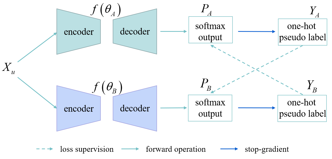
Figure 1: Illustrating the architectures for consistent learning.

2 Method

2.1 Consistency-based learning

As shown in Figure 1, let the $X_{l}=\{x_{li},i\in N\}$ and $X_{u}=\{x_{ui},i\in M\}$ be the labeled and unlabeled data, respectively, where $N$ and $M$ are the number of labeled and unlabeled data, respectively. In our experiment, the condition of $\ll M$ is established for semi-supervised learning. First, dual identical networks $f(\theta_{A})$ and $f(\theta_{B})$ are built with different parameter initialization methods. Then, dual identical networks $f(\theta_{A})$ and $f(\theta_{B})$ are trained by using the labeled data for abdominal organ segmentation, respectively.

$$f(x_{li};\theta_{A})=p_{A,li}$$ (1)

$$f(x_{li};\theta_{B})=p_{B,li}$$

where $p$ is the probability map. Next, the trained network is used to obtain different probability map of unlabeled data and their pseudo-labels.

$$f(x_{ui};\theta_{A})=p_{A,ui},f(x_{uj};\theta_{A})=p_{A,uj}$$ (2)

$$f(x_{ui};\theta_{B})=p_{B,ui},f(x_{uj};\theta_{B})=p_{B,uj}$$

$$y_{A,ui}=\text{argmax}(p_{A,ui}),y_{A,uj}=\text{argmax}(p_{A,uj})$$ (3)

$$y_{B,ui}=\text{argmax}(p_{A,ui}),y_{B,uj}=\text{argmax}(p_{B,uj})$$

CutMix operation [14] is implemented on different unlabeled data and pseudo labels:

$$x_{uij}=\mathbf{H}\odot x_{ui}+(1-\mathbf{H})\odot x_{uj}$$ (4)

$$y_{A,uij}=\mathbf{H}\odot y_{A,ui}+(1-\mathbf{H})\odot y_{A,uj}$$

$$y_{B,uij}=\mathbf{H}\odot y_{B,ui}+(1-\mathbf{H})\odot y_{B,uj}$$

In this situation, the outputs of the two networks can be used to supervise for each other, which achieves the network consistency-based learning.

$$f(x_{uij};\theta_{A})=p_{A,uij}\longrightarrow y_{B,uij}$$ (5)

$$f(x_{uij};\theta_{B})=p_{B,uij}\longrightarrow y_{A,uij}$$

2.2 Light UNet

To accelerate inference speed and reduce the GPU memory utilization, we modify the UNet in nnU-Net[9]. A light UNet was presented in Figure 2.

• We replace the original convolution with depthwise separable convolution [3], thus reducing the number of trainable parameters.

• Residual connection [5] was introduced between all convolution layers, including encoder and decoder, thus improving the representational ability of the UNet.

Figure 2: The architecture of Light UNet.

2.3 Robust segmentation Loss

In the segmentation task, the commonly used segmentation loss is a combination of Dice loss and cross entropy (CE) loss, which have been proved be robust in various medical image segmentation task [11]. In this paper, based on the previous segmentation loss, the idea of mean absolute error (MAE) loss was introduced into Dice and CE loss respectively. Therefore, a robust segmentation loss fuction $\mathcal{L}_{RS}$ was proposed, which consists of noise robust dice loss $\mathcal{L}_{NRD}$ and taylor cross entropy loss $\mathcal{L}_{TCE}$.

$$\mathcal{L}_{RS}=\mathcal{L}_{NRD}+\mathcal{L}_{TCE}$$ (6)

$$\mathcal{L}_{NRD}=\frac{\sum_{n=1}^{DWH}|\mu_{n}-\upsilon_{n}|^{\gamma}}{\sum_{n=1}^{DWH}\mu_{n}^{2}+\sum_{n=1}^{DWH}\upsilon_{n}^{2}+\epsilon}$$ (7)

$$\mathcal{L}_{TCE}=\sum_{n=1}^{DWH}(1-\mu_{n,\upsilon=1})+\frac{\sum_{n=1}^{DWH}(1-\mu_{n,\upsilon=1})^{2}}{2}$$ (8)

where $D$, $W$ and $H$ are the depth, width and height of input, respectively. $\mu$ and $\upsilon$ are the voxels of softmax output and ground truth, respectively.

2.4 Preprocessing

The dataset was preprocessed by nnU-Net configuration. In order to achieve category-balanced cropping in unlabeled data, a nnU-Net model was trained in advance using a small amount of labeled data. Then, a pseudo-label for unlabeled data is generated, which is only involved in achieving category-balanced cropping and not in other utilization.

3 Experiments

3.1 Dataset and evaluation measures

The FLARE2022 dataset is curated from more than 20 medical groups under the license permission, including MSD [13], KiTS [7, 8], AbdomenCT-1K [12], and TCIA [4]. The training set includes 50 labelled CT scans with pancreas disease and 2000 unlabelled CT scans with liver, kidney, spleen, or pancreas diseases. The validation set includes 50 CT scans with liver, kidney, spleen, or pancreas diseases. The testing set includes 200 CT scans where 100 cases has liver, kidney, spleen, or pancreas diseases and the other 100 cases has uterine corpus endometrial, urothelial bladder, stomach, sarcomas, or ovarian diseases. All the CT scans only have image information and the center information is not available.

The evaluation measures consist of two accuracy measures: Dice Similarity Coefficient (DSC) and Normalized Surface Dice (NSD), and three running efficiency measures: running time, area under GPU memory-time curve, and area under CPU utilization-time curve. Only DSC score was presented in the experiments. All measures will be used to compute the ranking. Moreover, the GPU memory consumption has a 2 GB tolerance.

3.2 Implementation details

3.2.1 Environment settings

The development environments and requirements are presented in Table 1.

Table 1: Development environments and requirements.

Windows/Ubuntu version	Ubuntu 18.04.5 LTS
CPU	Intel(R) Xeon(R) Gold 5218 CPU @ 2.30GHz
RAM	503 GB
GPU (number and type)	Two NVIDIA RTX 2080Ti 11G
CUDA version	11.0
Programming language	Python 3.7
Deep learning framework	Pytorch (Torch 1.11, torchvision 0.2.2)

3.2.2 Training protocols

Ther training protocols are presented in Table 2

Table 2: Training protocols.

Network initialization	“he" normal initialization
Batch size	1
Patch size	56$\times$160$\times$160
Target resolution	2.5$\times$1.5$\times$1.5
Total epochs	1000
Optimizer	SGD with nesterov momentum ($\mu=0.99$)
Initial learning rate (lr)	0.01
Lr decay schedule	halved by 200 epochs
Training time	276 hours
Loss function	RRD + TCE
Number of model parameters	5.59M
Number of flops	33.81G

4 Results and discussion

A public unlabeled validation set was used to evaluate the experiment results, which can be uploaded to the online for metrics.

4.1 Ablation of semi-supervised learning

Table 3 shows the effects of introducing semi-supervised learning in the nnU-Net and light unet on the final segmentation performance, respectively. Two conclusions can be found from Table 3: (1) The segmentation performance of the light unet is inferior to the nnU-Net due to the less parameters, but the light unet can speed up the inference and reduce the GPU memory utilization. (2) The introduction of semi-supervised learning has greatly improved the segmentation performance for both. Further, the performance improvement is greater for the light unet with a smaller number of parameters than nnU-Net, which may be caused by model with few parameters has strong potential for improvement.

Table 3: Ablation of semi-supervised learning (SSL). LV, RK, SL, PC, AT, IVC, RAG, LAG, GB, EH, SM, DD, and LK are short for Liver, Right Kidney, Spleen, Pancreas, Aorta, Inferior Vena Cava, Right Adrenal Gland, Left Adrenal Gland, Gallbladder, Esophagus, Stomach, and Left kidney, respectively.

Method	Mean	LV	RK	SL	PC	AT	IVC	RAG	LAG	GB	EH	SM	DD	LK
nnU-Net w/o SSL	0.869	0.967	0.880	0.941	0.841	0.949	0.882	0.822	0.819	0.821	0.877	0.885	0.748	0.871
nnU-Net w SSL	0.895	0.978	0.897	0.973	0.909	0.973	0.922	0.839	0.826	0.779	0.900	0.914	0.838	0.888
Light UNet w/o SSL	0.837	0.965	0.869	0.932	0.830	0.945	0.860	0.766	0.731	0.731	0.837	0.858	0.717	0.843
Light UNet w SSL	0.878	0.976	0.910	0.969	0.894	0.960	0.896	0.807	0.763	0.764	0.865	0.915	0.799	0.891

Table 4: Comparison of loss function.

Loss	Mean	LV	RK	SL	PC	AT	IVC	RAG	LAG	GB	EH	SM	DD	LK
Dice+CE	0.869	0.972	0.915	0.954	0.861	0.958	0.884	0.823	0.814	0.720	0.867	0.888	0.751	0.889
NRD+TCE	0.870	0.967	0.880	0.941	0.841	0.949	0.882	0.822	0.819	0.821	0.877	0.885	0.748	0.871

4.2 Comparison of loss function

From Table Table 4, it can be found that the robust segmentation loss is superior to the combination of dice and CE loss in terms of overall performance. Moreover, it can be noticed that although the robust segmentation loss is inferior to the combination of dice and CE loss for the segmentation of most organs from the segmentation performance of different organs, the robust segmentation loss has a great advantage for the segmentation of the gallbladder. The gallbladder belongs to the small target segmentation region, therefore, we conclude that robust segmentation loss has some advantages for the small target region.

4.3 Segmentation efficiency results

Considering the balance between segmentation performance and inference speed, we reduce the original 7 times flips in nnU-net to 3 tmes flips (tta). Moreover, in order to address the phenomenon that particularly large samples in the image will be out of memory during the inference process, we only keep the final generated labels and do not keep the intermediate network output (RAM). The result was performed in Table 5.

We did not upload docker to test computational efficiency issues. However, we tested on our own platform to test the optimization of computational efficiency. In the end, we achieved a test time of 0.67 hour on 50 validation samples, maximum ram is 18G, and GPU memory is 2045MB.

Table 5: Extra Processing for fianl result. IS(H) is short for inference speed, with hour as unit.

Method	Mean	IS(H)	LV	RK	SL	PC	AT	IVC	RAG	LAG	GB	EH	SM	DD	LK
DLUNet	0.878		0.976	0.910	0.969	0.894	0.960	0.896	0.807	0.763	0.764	0.865	0.915	0.799	0.891
DLUNet+tta	0.884	2.00	0.977	0.910	0.972	0.899	0.962	0.901	0.816	0.762	0.801	0.873	0.917	0.800	0.895
DLUNet+tta+RAM	0.872	0.67	0.973	0.903	0.964	0.890	0.948	0.888	0.789	0.741	0.792	0.857	0.911	0.795	0.885

4.4 Qualitative results

Figure 3 presents some easy and hard examples on validation set, and quantitative result is illustrated in Table 6. Comparing (Case 06 and Case 21) and (Case 47 and Case 48), we can find that our proposed method does not work well for lesion-affected organs. For example, the liver cancer region is wrongly identified in Case 47 and Case 48, especially Case 48. This situation may be due to our proposed method is implemented by a patch-based training strategy, which lacks global information.

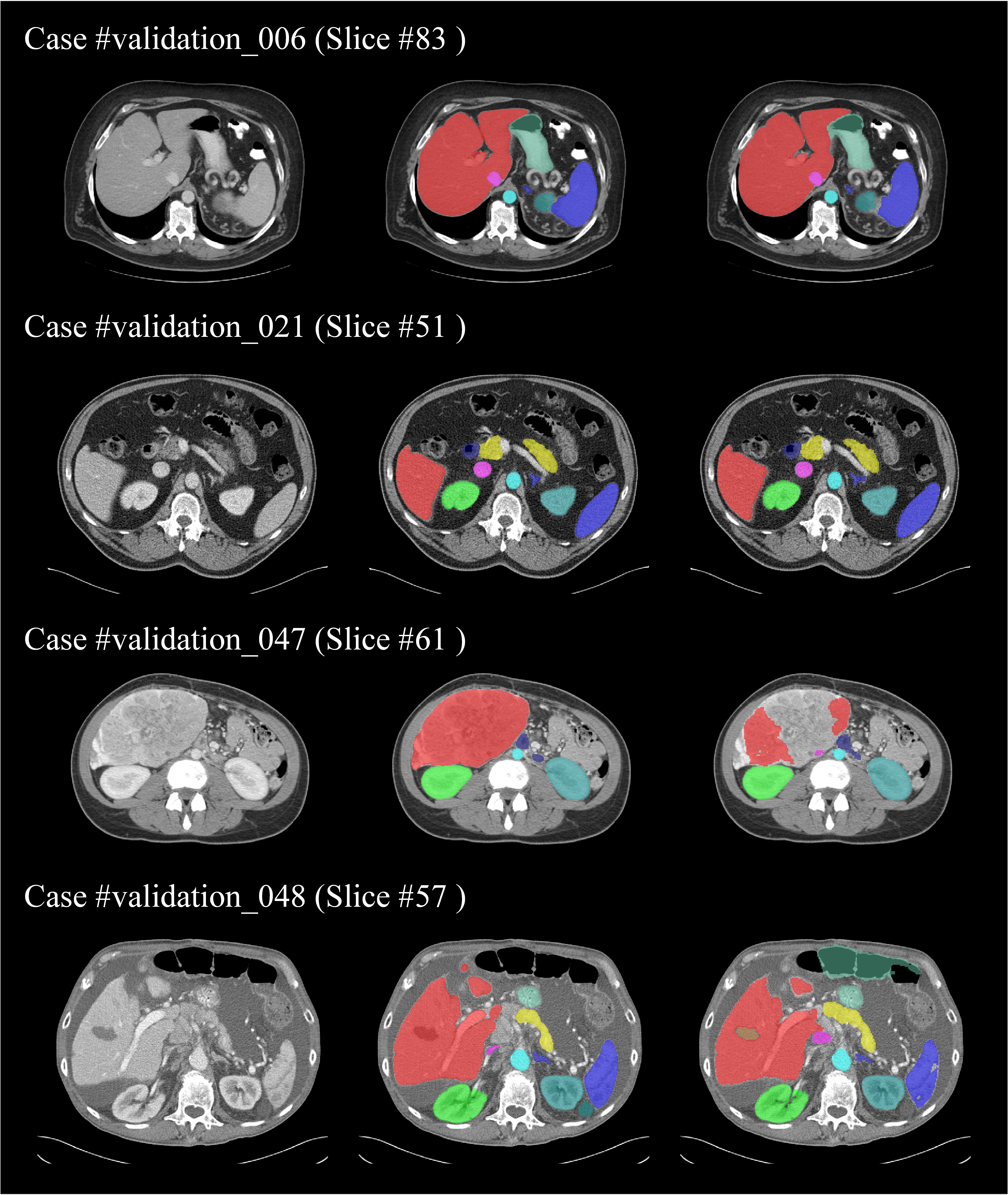
Figure 3: Qualitative results on easy (case 06 and 21) and hard (case 47 and 48) examples. First column is the image, second column is the ground truth, and third column is the predicted results by DLUNet.

Table 6: The DSC scores of easy and hard examples.

Example	Mean	LV	RK	SL	PC	AT	IVC	RAG	LAG	GB	EH	SM	DD	LK
Case 06	0.915	0.983	0.974	0.978	0.924	0.965	0.944	0.899	0.894	1.000	0.908	0.936	0.756	0.729
Case 21	0.946	0.985	0.972	0.983	0.926	0.966	0.937	0.869	0.864	1.000	0.935	0.969	0.926	0.973
Case 47	0.798	0.885	0.978	0.866	0.798	0.936	0.665	0.677	0.818	0.676	0.807	0.904	0.395	0.977
Case 48	0.716	0.971	0.971	0.667	0.841	0.958	0.461	0.679	0.856	0.000	0.693	0.598	0.796	0.811

4.5 Limitation and future work

In this paper, we do not use existing deep learning model packaging techniques (e.g., TensorRT) to package the model, reduce computational memory, and increase inference speed. Therefore, the implementation of the operation can be considered in the future work.

5 Conclusion

The FLARE2022 competition aims to design an efficient and accuracy abdominal multi-organ segmentation network by using a small amount of labeled data and a large amount of unlabeled data. In this paper, we proposed DLUNet for this task. First, consistent-based learning was introduced to achieve semi-supervised learning. Second, separable convolution and residual connection were used to greatly reduce the computational cost. Moreover, a robust segmentation loss was applied to improve segmentation performance. Experiments prove that the DLUNet achieves a certain balance in terms of model parameters, computation time, GPU memory utilization, and segmentation performance. The method is promising for the task.

5.0.1 Acknowledgements

The authors of this paper declare that the segmentation method they implemented for participation in the FLARE 2022 challenge has not used any pre-trained models nor additional datasets other than those provided by the organizers. The proposed solution is fully automatic without any manual intervention.

References

- [1] Arazo, E., Ortego, D., Albert, P., O’Connor, N.E., McGuinness, K.: Pseudo-labeling and confirmation bias in deep semi-supervised learning. In: 2020 International Joint Conference on Neural Networks (IJCNN). pp. 1–8. IEEE (2020)
- [2] Chen, X., Yuan, Y., Zeng, G., Wang, J.: Semi-supervised semantic segmentation with cross pseudo supervision. In: IEEE Conference on Computer Vision and Pattern Recognition, CVPR 2021, virtual, June 19-25, 2021. pp. 2613–2622. Computer Vision Foundation / IEEE (2021), https://openaccess.thecvf.com/content/CVPR2021/html/Chen_Semi-Supervised_Semantic_Segmentation_With_Cross_Pseudo_Supervision_CVPR_2021_paper.html
- [3] Chollet, F.: Xception: Deep learning with depthwise separable convolutions. In: Proceedings of the IEEE conference on computer vision and pattern recognition. pp. 1251–1258 (2017)
- [4] Clark, K., Vendt, B., Smith, K., Freymann, J., Kirby, J., Koppel, P., Moore, S., Phillips, S., Maffitt, D., Pringle, M., et al.: The cancer imaging archive (tcia): maintaining and operating a public information repository. Journal of Digital Imaging 26(6), 1045–1057 (2013)
- [5] He, K., Zhang, X., Ren, S., Sun, J.: Deep residual learning for image recognition. In: Proceedings of the IEEE conference on computer vision and pattern recognition. pp. 770–778 (2016)
- [6] He, R., Yang, J., Qi, X.: Re-distributing biased pseudo labels for semi-supervised semantic segmentation: A baseline investigation. In: Proceedings of the IEEE/CVF International Conference on Computer Vision. pp. 6930–6940 (2021)
- [7] Heller, N., Isensee, F., Maier-Hein, K.H., Hou, X., Xie, C., Li, F., Nan, Y., Mu, G., Lin, Z., Han, M., et al.: The state of the art in kidney and kidney tumor segmentation in contrast-enhanced ct imaging: Results of the kits19 challenge. Medical Image Analysis 67, 101821 (2021)
- [8] Heller, N., McSweeney, S., Peterson, M.T., Peterson, S., Rickman, J., Stai, B., Tejpaul, R., Oestreich, M., Blake, P., Rosenberg, J., et al.: An international challenge to use artificial intelligence to define the state-of-the-art in kidney and kidney tumor segmentation in ct imaging. American Society of Clinical Oncology 38(6), 626–626 (2020)
- [9] Isensee, F., Jaeger, P.F., Kohl, S.A., Petersen, J., Maier-Hein, K.H.: nnu-net: a self-configuring method for deep learning-based biomedical image segmentation. Nature Methods 18(2), 203–211 (2021)
- [10] Luo, X., Chen, J., Song, T., Wang, G.: Semi-supervised medical image segmentation through dual-task consistency. CoRR abs/2009.04448 (2020), https://arxiv.org/abs/2009.04448
- [11] Ma, J., Chen, J., Ng, M., Huang, R., Li, Y., Li, C., Yang, X., Martel, A.L.: Loss odyssey in medical image segmentation. Medical Image Analysis 71, 102035 (2021)
- [12] Ma, J., Zhang, Y., Gu, S., Zhu, C., Ge, C., Zhang, Y., An, X., Wang, C., Wang, Q., Liu, X., Cao, S., Zhang, Q., Liu, S., Wang, Y., Li, Y., He, J., Yang, X.: Abdomenct-1k: Is abdominal organ segmentation a solved problem? IEEE Transactions on Pattern Analysis and Machine Intelligence (2021). https://doi.org/10.1109/TPAMI.2021.3100536
- [13] Simpson, A.L., Antonelli, M., Bakas, S., Bilello, M., Farahani, K., Van Ginneken, B., Kopp-Schneider, A., Landman, B.A., Litjens, G., Menze, B., et al.: A large annotated medical image dataset for the development and evaluation of segmentation algorithms. arXiv preprint arXiv:1902.09063 (2019)
- [14] Yun, S., Han, D., Oh, S.J., Chun, S., Choe, J., Yoo, Y.: Cutmix: Regularization strategy to train strong classifiers with localizable features. In: Proceedings of the IEEE/CVF international conference on computer vision. pp. 6023–6032 (2019)