Inferring neutron star properties with continuous gravitational waves

Abstract

Detection of continuous gravitational waves from rapidly-spinning neutron stars opens up the possibility of examining their internal physics. We develop a framework that leverages a future continuous gravitational wave detection to infer a neutron star’s moment of inertia, equatorial ellipticity, and the component of the magnetic dipole moment perpendicular to its rotation axis. We assume that the neutron star loses rotational kinetic energy through both gravitational wave and electromagnetic radiation, and that the distance to the neutron star can be measured, but do not assume electromagnetic pulsations are observable or a particular neutron star equation of state. We use the Fisher information matrix and Monte Carlo simulations to estimate errors in the inferred parameters, assuming a population of gravitational-wave-emitting neutron stars consistent with the typical parameter domains of continuous gravitational wave searches. After an observation time of one year, the inferred errors for many neutron stars are limited chiefly by the error in the distance to the star. The techniques developed here will be useful if continuous gravitational waves are detected from a radio, X-ray, or gamma-ray pulsar, or else from a compact object with known distance, such as a supernova remnant.

1 Introduction

The field of gravitational wave astronomy, while relatively new, has the potential to make exciting contributions to many areas of astrophysics. The first gravitational wave event, GW150914, was detected in 2015 and was generated by a binary black hole merger (Abbott et al., 2016). Since this first detection, the Laser Interferometer Gravitational-Wave Observatory (LIGO) (Aasi et al., 2015) and Virgo (Acernese et al., 2015) gravitational wave observatories have made almost 100 confirmed detections (Abbott et al., 2021a). The KAGRA detector (Akutsu et al., 2019) also operated during the later portion of the O3b observing run (Akutsu et al., 2020).

Gravitational wave detection allows for multi-messenger astronomy if an event is simultaneously observed in both electromagnetic and gravitational wave bands. This was successfully achieved in 2017 with the detection of GW170817, a gravitational wave event generated by a binary neutron star merger, which was also independently observed as the gamma ray burst GRB170817a across the electromagnetic spectrum (Abbott et al., 2017a, b). Gravitational wave and multi-messenger astronomy will likely be the source of many future discoveries as gravitational wave detector sensitivity increases and more detectors come online.

Gravitational wave astronomy has the potential to advance our understanding of neutron stars and the physics of matter at extreme densities. Gravitational waves from neutron star mergers are detectable by current ground-based observatories, but only for a short time at the end of their life cycle when their stellar structure is tidally deformed.

Continuous gravitational waves are long-lived, quasi-monochromatic gravitational waves emitted by isolated spinning neutron stars that are deformed asymmetrically about their rotation axes. The deformation may be caused by a number of mechanisms, including the neutron star’s magnetic field (Zimmermann & Szedenits, 1979; Bonazzola & Gourgoulhon, 1996), magnetically-confined mountains (Melatos & Payne, 2005), or electron capture gradients (Ushomirsky et al., 2000). The stellar structure is expected to be in a long-lived stable equilibrium and continuous gravitational waves (hereafter abbreviated to “continuous waves”) could provide insights into the ground state of nuclear matter complementary to observations of binary neutron star mergers.

While continuous waves have not yet been detected, prospects for a first detection continue to improve with more sensitive gravitational wave detectors. In addition, the data analysis techniques used to search for continuous wave signals continue to be refined; for reviews see Riles (2013, 2017); Tenorio et al. (2021). Searches for continuous waves cover a wide variety of sources and include: known radio and X-ray pulsars (Abbott et al., 2020b, 2021d, 2021f, 2022a, 2022d, 2022e), likely neutron stars in supernova remnants (Abbott et al., 2021e, 2022c), and all-sky surveys for undiscovered neutron stars (Abbott et al., 2021b, c, 2022b; Covas et al., 2022).

In this paper, we study what macroscopic properties of neutron stars might be inferred using continuous waves. Sieniawska & Jones (2022) have previously studied this question under the assumption that the neutron star loses rotational kinetic energy purely through gravitational wave radiation. Here we consider a more general model where energy is also lost through electromagnetic radiation, assuming the star possesses a dipolar magnetic field. The population dynamics of neutron stars losing energy through both electromagnetic and gravitational radiation have previously been studied by Palomba (2005); Knispel & Allen (2008); Wade et al. (2012); Cieślar et al. (2021); Reed et al. (2021). This paper is an initial attempt at studying the parameter estimation problem for such systems.

This paper is organised as follows. Section 2 introduces background information on continuous waves and their detection. Section 3 introduces the theoretical framework used to infer properties of the neutron star. Section 4 discusses how Monte Carlo simulations are used to estimate the errors of the inferred properties. Section 5 presents the results of the Monte Carlo simulations. Section 6 considers some of the caveats and assumptions, and Section 7 summarises the results.

2 Background

This section presents background information relevant to the paper. Subsections 2.1 and 2.2 introduce the basics of the signal model and parameter estimation techniques respectively for continuous wave searches.

2.1 Continuous wave signal model

A continuous wave induces a strain $h(t)$ in a gravitational wave detector given by (Jaranowski et al., 1998):

$$h(t)=\sum_{i=1}^{4}\mathcal{A}_{i}h_{i}(t;\vec{\lambda})\,.$$ (1)

The four amplitudes $\{\mathcal{A}_{i}\}$ are functions of: the characteristic strain amplitude $h_{0}$, the inclination angle $\iota$ of the neutron star’s angular momentum to the line of sight, a polarisation angle $\psi$ which fixes the principal axes of the two gravitational wave polarisations (“plus” and “cross”), and an arbitrary phase $\phi_{0}$ at a reference time $t_{0}$. Additional parameters, represented by $\vec{\lambda}$ in Eq. (1), modify the phase of the signal; they include the star’s sky position and, if the star is in a binary system, its orbital parameters.

The characteristic strain amplitude $h_{0}$ of a continuous wave signal is (Jaranowski et al., 1998):

$$h_{0}=\frac{4\pi^{2}G}{c^{4}}\frac{I_{zz}\epsilon f^{2}}{r}\,,$$ (2)

where $r$ is the distance to the neutron star, $f$ is the gravitational wave frequency, $G$ is the gravitational constant, and $c$ is the speed of light. We model the neutron star as a tri-axial rotor (Zimmermann & Szedenits, 1979) with principal moments of inertia $(I_{xx},I_{yy},I_{zz})$, where the $z$ axis points along the star’s symmetry rotation axis; the equatorial ellipticity $\epsilon=|I_{xx}-I_{yy}|/I_{zz}$ characterises the degree of non-axisymmetrical deformation of the star. For a tri-axial rotor the gravitational wave frequency is conventionally assumed to be twice the star’s rotational frequency (Van Den Broeck, 2005; Sieniawska & Jones, 2022).

The radiation of rotational kinetic energy away from the neutron star via continuous waves, and possibly electromagnetic radiation, causes the star to spin down. We model the evolution of the gravitational wave frequency as a second-order Taylor expansion (Jaranowski et al., 1998):

$$f(t)=f+\dot{f}t+\frac{1}{2}\ddot{f}t^{2}\,,$$ (3)

where $f$ is the gravitational wave frequency and $\dot{f}$ and $\ddot{f}$ its first and second time derivatives respectively, where all three parameters are defined at $t=t_{0}$. These parameters enter into Eq. (1) as phase parameters represented by $\vec{\lambda}$.

A useful quantification of the spin-down behaviour of a neutron star is its braking index (Manchester et al., 1985):

$$n=\frac{f\ddot{f}}{\dot{f}^{2}}\,.$$ (4)

If a neutron star is spinning down purely through the emission of gravitational waves from a (mass-type) quadrupole moment, as given by Eq. (2), its braking index is $n=5$; alternately, if the neutron star spins down only through electromagnetic radiation, its braking index is $n=3$ (Ostriker & Gunn, 1969) but cf. (Melatos, 1997). A third possibility, which we do not consider in this paper, is the emission of gravitational waves from a current-type quadrupole moment due to $r$-modes (Andersson, 1998; Lindblom et al., 1998), for which one has $n=7$.

2.2 Continuous wave parameter estimation

Detection of a continuous wave signal would measure its amplitude and phase to some degree of uncertainty, assuming that the true continuous wave signal does not deviate appreciably from the model described in section 2.1. Bayesian inference is widely regarded as a robust method of inferring parameters of a signal model given a data-set and assumed priors on the parameters; for its application to continuous waves see Dupuis & Woan (2005); Pitkin et al. (2017).

As an initial attempt to study the errors in the parameters measured by a continuous wave detection, we instead adopt a simpler approach using the Fisher information matrix. While this approach is commonly used (Sieniawska & Jones, 2022; Jaranowski & Królak, 1999), the Fisher information matrix is strictly valid only in the case of high signal-to-noise ratios (a criterion for which is detailed in Vallisneri 2008), which may not necessarily be the case for a first continuous wave detection. Further discussion of the weaknesses of the Fisher information matrix approach, such as the possibility of singular or ill-conditioned Fisher information matrices, are outlined in Vallisneri (2008). Notwithstanding these concerns, we use the Fisher information matrix because of its relative computational simplicity to arrive at a quantitative picture of parameter inference for continuous wave signals. We now outline how Fisher information matrices can be used to approximate the error of the continuous wave parameters.

Data analysis techniques that seek to identify continuous waves often quantify how closely an observed signal matches a template of possible signals. An intuitive picture of how the Fisher information matrix works is that it quantifies the maximal possible “distance” in the parameter space that a true signal could be from the “nearest” template. That is, since the template bank forms a “grid” (which may not be uniform) in the parameter space, the maximal error of the parameter measurements comes from the size of the “gaps” in the template bank.

As will become clear in Section 3, we are particularly interested in estimating errors in the three parameters $f$, $\dot{f}$, and $\ddot{f}$ of Eq. (3) which govern the gravitational wave frequency evolution. To construct the Fisher information matrix for these parameters, we start with phase of the continuous wave signal:

$$\phi_{\text{spin}}(t) =2\pi\int_{0}^{t}f(t^{\prime})dt^{\prime}\,,$$ (5)

$$=2\pi\left[ft+\frac{1}{2}\dot{f}(t)t^{2}+\frac{1}{6}\ddot{f}(t)t^{3}\right]\,,$$ (6)

where Eq. (3) has been substituted into Eq (5). We next compute the parameter-space metric (Balasubramanian et al., 1996; Owen, 1996) which quantifies the notion of “distance” between the true signal and a template. It is necessary to first define the time average operator:

$$\Big{\langle}x(t)\Big{\rangle}=\frac{1}{T}\int_{-T/2}^{T/2}x(t)dt\,,$$ (7)

where $x(t)$ is an arbitrary function and $T$ is the time span of the gravitational wave observation. The parameter-space metric over $f$, $\dot{f}$, and $\ddot{f}$ is then given by (Brady et al., 1998; Prix, 2007)

$$:g_{ij}=\Bigg{\langle}\frac{\partial\phi_{\text{spin}}(t)}{\partial f^{(i)}}\frac{\partial\phi_{\text{spin}}(t)}{\partial f^{(j)}}\Bigg{\rangle}-\Bigg{\langle}\frac{\partial\phi_{\text{spin}}(t)}{\partial f^{(i)}}\Bigg{\rangle}\Bigg{\langle}\frac{\partial\phi_{\text{spin}}(t)}{\partial f^{(j)}}\Bigg{\rangle}\,,$$ (8)

with $i,j\in\{0,1,2\}$, $f^{(0)}=f$, $f^{(1)}=\dot{f}$, and $f^{(2)}=\ddot{f}$.

The covariance matrix for $f$, $\dot{f}$, and $\ddot{f}$ is given by the inverse Fisher information matrix $\Gamma^{ij}$ (Vallisneri, 2008), which, in turn, is defined in terms of the parameter-space metric (Prix, 2007):

$$\Sigma(f,\dot{f},\ddot{f}) =\Gamma^{ij}$$ (9)

$$=\frac{g^{ij}}{\rho^{2}}\,.$$ (10)

Here $\rho^{2}$ is the signal-to-noise ratio assuming an optimal match between the true signal and the best-fit template. For observation times of a year or more, we can assume an expression for $\rho^{2}$ averaged over $\cos\iota$, $\psi$, and sky position (Jaranowski et al., 1998; Prix, 2011):

$$\rho^{2} =\frac{4}{25}\frac{h_{0}^{2}T}{S_{h}(f)}\,,$$ (11)

$$=\frac{4}{25}\frac{T}{\mathcal{D}^{2}}\,,$$ (12)

where $S_{h}$ is the (single-sided) power spectral density of the strain noise in the gravitational wave detector, and Eq. (12) defines the "sensitivity depth" (Behnke et al., 2015; Dreissigacker et al., 2018):

$$\mathcal{D}=\frac{\sqrt{S_{h}(f)}}{h_{0}}\,,$$ (13)

We assume, again for simplicity, that the gravitational wave detector network is operational at 100% duty cycle; in practice duty cycles of $\gtrsim 70\%$ are achieved for current detectors, but this is expected to improve over time (Abbott et al., 2020a). Evaluating Eq. (9) using Eqs. (6) and (8) gives the covariance matrix:

$$\Sigma(f,\dot{f},\ddot{f}) =\frac{\mathcal{D}^{2}}{\pi^{2}}\begin{pmatrix}\frac{1875}{16T^{3}}&0&-\frac{7875}{2T^{5}}\\ 0&\frac{1125}{T^{5}}&0\\ -\frac{7875}{2T^{5}}&0&\frac{157500}{T^{7}}\end{pmatrix}\,.$$ (14)

Now considering the four amplitude parameters $h_{0}$, $\cos\iota$, $\psi$, $\phi_{0}$; only $h_{0}$ is potentially interesting for inferring neutron star properties as it is a function of $I_{zz}$ and $\epsilon$ [Eq. (2)]. The error in the $h_{0}$ measurement may be derived from the parameter-space metric over the amplitude parameters $\{\mathcal{A}_{i}\}$ (Prix, 2007), as outlined in Prix (2011, Section 3.2). For year-long observations, it is conventional to consider the error in $h_{0}$ averaged over sky position (Prix, 2011, Eq. 122) and $\psi$:

$$\sigma(h_{0}) =\frac{a\mathcal{D}h_{0}}{\sqrt{T}}\frac{\sqrt{b+\xi^{2}}}{1-\xi^{2}}\,,$$ (15)

$$\xi \equiv\cos\iota\,,$$ (16)

$$a =2\sqrt{\frac{6}{301}\left(344-43\sqrt{2}-8\sqrt{86}\right)}\approx 4.08\,,$$ (17)

$$b =\frac{43\left(8-8\sqrt{2}-\sqrt{86}\right)}{43\sqrt{2}+8\sqrt{86}-344}\approx 2.59\,.$$ (18)

Note that Eq. (15) becomes infinite at $\xi=\pm 1$, due to a singularity in the coordinate transform between $\{\mathcal{A}_{i}\}$ and $\{h_{0},\xi,\psi,\phi_{0}\}$; for this reason Eq. (15) cannot be analytically averaged over $\xi$ with a prior range that includes $\pm 1$.

3 Parameter estimation framework

This section develops a framework for inferring three neutron star properties: its principal moment of inertia ($I_{zz}$), its ellipticity ($\epsilon$), and the component of the magnetic dipole moment perpendicular to its rotation axis ($m_{p}$, hereafter abbreviated to “perpendicular magnetic moment”). It assumes that the neutron star is losing rotational kinetic energy (and hence spinning down) through both magnetic dipole radiation and gravitational wave (mass-type) quadrupolar radiation, and that no other mechanisms dissipate energy from the neutron star. This framework relies on the detection of a continuous wave signal to measure the frequency and spin-down parameters ($f$, $\dot{f}$, and $\ddot{f}$), and the characteristic strain amplitude ($h_{0}$). It also assumes that a measurement of the distance to the neutron star ($r$) is available.

Balancing the spin-down power with the luminosity of electromagnetic and gravitational radiation gives:

$$\left(\frac{dE}{dt}\right)_{\text{EM}}+\left(\frac{dE}{dt}\right)_{\text{GW}}=-\left(\frac{dE}{dt}\right)_{\text{rot}}\,.$$ (19)

The ellipticity of a neutron star is conventionally assumed to be relatively small (Sieniawska & Jones, 2022), so the star is very close to spherical. The rotational kinetic energy of the star is then taken to be that of a rotating sphere (Wette et al., 2008):

$$\Bigg{(}\frac{dE}{dt}\Bigg{)}_{\text{rot}}=\pi^{2}I_{zz}f\dot{f}\,.$$ (20)

The luminosity of a rotating magnetic dipole is (Ostriker & Gunn, 1969; Condon & Ransom, 2016)

$$\left(\frac{dE}{dt}\right)_{\text{EM}}=\frac{2m_{p}^{2}}{3c^{3}\mu_{0}}(\pi f)^{4}\,,$$ (21)

where $\mu_{0}$ is the vacuum permeability. Note that this is given in terms of the gravitational wave frequency which is twice the rotational frequency as discussed in Section 2.1. The gravitational wave luminosity of a (mass-type) quadrupole is (Ostriker & Gunn, 1969; Blanchet et al., 2001)

$$\Bigg{(}\frac{dE}{dt}\Bigg{)}_{\text{GW}}=\frac{32G}{5c^{5}}I_{zz}^{2}\epsilon^{2}(\pi f)^{6}\,.\$$ (22)

In order to simplify the expressions, we introduce the constants

$$K_{\text{EM}}=\frac{2\pi^{2}}{3c^{3}\mu_{0}}\,,\qquad K_{\text{GW}}=\frac{32G\pi^{4}}{5c^{5}}\,.$$ (23)

We then substitute Eqs. (20) – (22) into Eq. (19) and rearrange to get:

$$\dot{f}=-\frac{K_{\text{EM}}m_{p}^{2}f^{3}}{I_{zz}}-K_{\text{GW}}I_{zz}\epsilon^{2}f^{5}\,.$$ (24)

Differentiating Eq. (24) with respect to time gives:

$$\ddot{f}=-\frac{3K_{\text{EM}}m_{p}^{2}f^{2}\dot{f}}{I_{zz}}-5K_{\text{GW}}I_{zz}\epsilon^{2}f^{4}\dot{f}\,.$$ (25)

Given that $\ddot{f}$ is measured as a separate parameter of the continuous wave signal model [Eq. (3)], Eq. (25) provides an additional constraint independent of Eq. (24).

Equations (24) and (25) depend on three unknowns: $I_{zz}$, $\epsilon$, and $m_{p}$. With the addition Equation. (2) which also depends on $I_{zz}$ and $\epsilon$, we have three equations constraining the same three unknowns which may now be solved for:

$$I_{zz} =\frac{K_{\text{GW}}c^{8}r^{2}h_{0}^{2}f}{8\pi^{4}G^{2}\dot{f}(3-n)}\,,$$ (26)

$$\epsilon =\frac{2\pi^{2}G\dot{f}(3-n)}{K_{\text{GW}}c^{4}rh_{0}f^{3}}\,,$$ (27)

$$m_{p} =\frac{c^{4}rh_{0}}{4\pi^{2}Gf}\sqrt{\frac{K_{\text{GW}}(n-5)}{K_{\text{EM}}(3-n)}}\,,$$ (28)

where $n$ is the braking index of Eq. (4). It is also possible to solve for the mass quadrupole moment of the neutron star (Owen, 2005):

$$Q_{22}=\sqrt{\frac{15}{8\pi}}I_{zz}\epsilon=\sqrt{\frac{15}{128\pi^{5}}}\frac{c^{4}rh_{0}}{Gf^{2}}\,.$$ (29)

Note that Eq. (29) has the nice property of being independent of $n$. Nevertheless, we choose to consider $I_{zz}$ and $\epsilon$ separately in this work to distinguish neutron star properties with relatively small ($I_{zz}$) and large ($\epsilon$) prior uncertainties (see Section 4.1).

Equations (26) – (28) remain valid provided that $3<n<5$, which is consistent with the power balance assumed by Eq. (19). As discussed in Section 2.1, braking indices of 3 or 5 correspond to pure electromagnetic or gravitational wave radiation respectively; in either case, Eqs. (26) – (28) are no longer applicable. A combination of electromagnetic and gravitational wave radiation yields a braking index between 3 and 5; the loss of kinetic rotational energy through both gravitational wave and electromagnetic radiation is therefore a fundamental requirement of the framework outlined here. Sieniawska & Jones (2022) show that, for a neutron star only emitting continuous waves and not electromagnetic radiation, degeneracies prevent direct inference of the neutron star properties without a measurement of $r$, which is unlikely to be measurable without an electromagnetic counterpart.

Few other techniques exist to directly measure $I_{zz}$. Damour & Schäeer (1988) propose a method which requires higher-order relativistic corrections to the periastron advance to be measurable, which is possible only for very rapidly-spinning binary pulsars. To date the method has only been applicable to the double pulsar system PSR J0737$-$3039 (Bejger et al., 2005; Worley et al., 2008; Steiner et al., 2015; Miao et al., 2022). Note that Miao et al. (2022) assumes a neutron star equation of state, whereas the framework derived here does not. Other methods rely on separate measurements of the neutron star mass and radius through either electromagnetic observations and/or detection of gravitational waves from binary neutron star mergers (Steiner et al., 2015; Miao et al., 2022). It is difficult, however, to measure both properties simultaneously for the one same neutron star (Miller et al., 2019). No method exists for directly measuring $\epsilon$ other than through a continuous wave detection. While $m_{p}$ (or equivalently the surface magnetic field strength $B$) is routinely inferred by assuming pure magnetic dipole radiation from known pulsars (Kramer, 2005), a measurement of $m_{p}$ from a mixed electromagnetic/gravitational wave pulsar would be of interest as it would provide an independent verification of the existing measurements or provide insight into neutron stars with different energy loss mechanisms.

The errors in the inferred neutron star properties ($I_{zz}$, $\epsilon$, $m_{p}$) has the following dependencies:

• The errors of the inferred properties ($\Delta I_{zz}$, $\Delta\epsilon$, and $\Delta m_{p}$) depend on $\Delta f$, $\Delta\dot{f}$, $\Delta\ddot{f}$, $\Delta h_{0}$, and $\Delta r$ [Eqs. (26) – (28)];

• The errors of the spindown parameters ($\Delta f$, $\Delta\dot{f}$, $\Delta\ddot{f}$) depend on $T$ and $\mathcal{D}$ [Eq. (12)];

• The error $\Delta h_{0}$ depends on $T$, $\mathcal{D}$, and $h_{0}$ [or equivalently $S_{h}$; Eq. (13)] and $\xi$ [Eq. (15)];

• The error $\Delta r$ is independent of the other parameters.

Therefore, we see that the errors in $I_{zz}$, $\epsilon$, $m_{p}$ depend entirely on: the observation time ($T$); the strength of the continuous wave signal relative to the detector noise ($\mathcal{D}$, $h_{0}$); the ratio of gravitational wave “plus” and “cross” polarisations ($\xi$); and the uncertainty in the distance to the star ($\Delta r$).

An estimate of the relative errors in $I_{zz}$, $\epsilon$, and $m_{p}$ and their dependence on the parameters $\Lambda=\{f,\dot{f},\ddot{f},h_{0},r\}$ may be arrived at through differential error analysis (Benke et al., 2018):

$$\frac{\sigma(I_{zz})^{2}}{I_{zz}^{2}}=\frac{1}{I_{zz}^{2}}\sum_{x,y\in\Lambda}\left(\frac{\partial I_{zz}}{\partial x}\right)\left(\frac{\partial I_{zz}}{\partial y}\right)\begin{cases}\sigma(x)^{2}&x=y\,,\\ \Sigma(x,y)&x\neq y\,,\end{cases}$$ (30)

and similarly for $\sigma(\epsilon)^{2}/\epsilon^{2}$ and $\sigma(m_{p})^{2}/m_{p}^{2}$; where $\sigma(x)$ is the standard deviation in the quantity $x$ and $\Sigma(x,y)$ is the covariance between the quantities $x$ and $y$. This analysis yields, to third order in $1/T$:

$$\frac{\sigma(I_{zz})^{2}}{I_{zz}^{2}} =\frac{4\sigma(r)^{2}}{r^{2}}+\frac{4\sigma(h_{0})^{2}}{h_{0}^{2}}+\frac{16875\mathcal{D}^{2}}{16\pi^{2}f^{2}(n-3)^{2}T^{3}}\,,$$ (31)

$$\frac{\sigma(\epsilon)^{2}}{\epsilon^{2}} =\frac{\sigma(r)^{2}}{r^{2}}+\frac{\sigma(h_{0})^{2}}{h_{0}^{2}}+\frac{1875\mathcal{D}^{2}(9-2n)^{2}}{16\pi^{2}f^{2}(n-3)^{2}T^{3}}\,,$$ (32)

$$\frac{\sigma(m_{p})^{2}}{m_{p}^{2}} =\frac{\sigma(r)^{2}}{r^{2}}+\frac{\sigma(h_{0})^{2}}{h_{0}^{2}}+\frac{1875\mathcal{D}^{2}(n^{2}-9n+15)^{2}}{16\pi^{2}f^{2}(n-5)^{2}(n-3)^{2}T^{3}}\,.$$ (33)

The leading-order terms of the relative errors in $I_{zz}$, $\epsilon$, and $m_{p}$ are the relative errors in $h_{0}$ and $r$. Note that $\sigma(r)/r$ is independent of $T$, $\sigma(h_{0})/h_{0}$ scales with $T^{-1/2}$ [Eq. (15)], and the remaining terms in Eqs. (31) – (33) scale with $T^{-3}$ or smaller. Since the distance error $\sigma(r)/r$ is assumed to be constant, in the limit of $T\to\infty$ the relative errors asymptote to:

$$\lim_{T\to\infty}\frac{\sigma(I_{zz})}{I_{zz}}=\frac{2\sigma(r)}{r}$$ (34)

$$\lim_{T\to\infty}\frac{\sigma(\epsilon)}{\epsilon}=\frac{\sigma(r)}{r}$$ (35)

$$\lim_{T\to\infty}\frac{\sigma(m_{p})}{m_{p}}=\frac{\sigma(r)}{r}$$ (36)

The asymptotic error in $I_{zz}$ is twice that of the other properties because the relationship between $I_{zz}$ and $r$ is $I_{zz}\propto r^{2}$ [Eq. (26)] whereas for the other two parameters it is $\epsilon\propto r^{-1}$ and $m_{p}\propto r$ [Eqs. (27) - (28)].

4 Monte Carlo simulations

The framework presented in Section 3 shows that it is possible to infer three neutron star properties using a continuous waves detection. In this section, we describe how Monte Carlo simulations were used to quantify to what accuracy these properties may be inferred with a detection.

The inference relies on five parameters ($f$, $\dot{f}$, $n$, $h_{0}$, $r$) [Eqs. (26) – (28)] and the errors of the inference depend on four additional parameters ($T$, $\mathcal{D}$, $\xi$, $\Delta r$) as well as $h_{0}$. In our simulations we choose to input values of $I_{zz}$ instead of $h_{0}$ through rearrangement of Eq (2). Results that directly depend on $h_{0}$ can be viewed as an optimistic or pessimistic case for the continuous wave signal detectability. In comparison, choices of $I_{zz}$ relate only to the neutron star’s internal physics. While larger values of $I_{zz}$ implicitly lead to a louder continuous wave signal, this also depends on the other neutron star parameters so does not relate as directly to the signal detectability.

The signal from a neutron star is simulated as the set of input values for the nine parameters ($f^{\text{in}}$, $\dot{f}^{\text{in}}$, $n^{\text{in}}$, $I_{zz}^{\text{in}}$, $r^{\text{in}}$, $T^{\text{in}}$, $\mathcal{D}^{\text{in}}$, $\xi^{\text{in}}$, $\Delta r^{\text{in}}$). The properties of the neutron star emitter $(I_{zz}^{\text{in}},\epsilon^{\text{in}},m_{p}^{\text{in}})$ can then be calculated using Eqs. (26)–(28). Measurement errors $(\delta f,\delta\ddot{f},\delta\ddot{f})$ in the simulated $f^{\text{in}},\dot{f}^{\text{in}},$ and $\ddot{f}^{\text{in}}$ (via $n^{\text{in}}$) are drawn from a multivariate normal distribution with covariance matrix given by Eq. (9); the measurement error $\delta h_{0}$ in $h_{0}^{\text{in}}$ is drawn from a normal distribution with standard deviation given by Eq. (15). All other covariances between the parameters $(f^{\text{in}},\dot{f}^{\text{in}},\ddot{f}^{\text{in}},h_{0}^{\text{in}})$ are assumed to be zero. The measured parameters of the continuous wave signal are then

$$f^{\text{out}} =f^{\text{in}}+\delta f\,, \dot{f}^{\text{out}} =\dot{f}^{\text{in}}+\delta\dot{f}\,,$$ (37)

$$\ddot{f}^{\text{out}} =\ddot{f}^{\text{in}}+\delta\ddot{f}\,, h_{0}^{\text{out}} =h_{0}^{\text{in}}+\delta h_{0}\,.$$

Substitution of $(f^{\text{out}},\dot{f}^{\text{out}},\ddot{f}^{\text{out}},h_{0}^{\text{out}})$ into Eqs. (2), (4) and (26) – (28) gives the inferred neutron star properties $(I_{zz}^{\text{out}},\epsilon^{\text{out}},m_{p}^{\text{out}})$, which may then be compared to $(I_{zz}^{\text{in}},\epsilon^{\text{in}},m_{p}^{\text{in}})$. We repeat this process for $10^{6}$ samples.

Below we describe the Monte Carlo procedure in further detail.

4.1 Choice of input parameters

Nine variables control the outputs of the Monte Carlo simulations: $f$, $\dot{f}$, $n$, $I_{zz}$, $r$, $T$, $\mathcal{D}$, $\xi$, $\Delta r$. We consider an observation time in the range of $T=0.5-4$ years. One can expect gravitational wave detector observing runs to last at least a year (Abbott et al., 2020a). A continuous wave signal detected in a year-long observing run may then be followed up in future and/or archival data.

The neutron star distance $r^{\text{in}}$ is fixed to $1\text{\,}\mathrm{k}\mathrm{p}\mathrm{c}$ for simplicity. Such a distance is within the range where all-sky continuous wave surveys are sensitive to neutron stars with ellipticities $\epsilon\gtrsim 10^{-6}$ and emitting at frequencies $f\gtrsim$100\text{\,}\mathrm{H}\mathrm{z}$$ (Abbott et al., 2021c). Given that the neutron star properties depend on the product $rh_{0}$ [Eqs. (26) – (28)], a choice of a smaller (larger) distance would be equivalent to simulating a larger (smaller) $h_{0}$. The fractional uncertainty in $r$ is chosen to be $\sigma(r)/r=20\%$. While radio pulsar distances (inferred through dispersion measures) exhibit appreciable variety and are susceptible to biases (Verbiest et al., 2012), a typical measurement uncertainty of $\sim 20\%$ is not unreasonable (Taylor & Cordes, 1993; Yao et al., 2017), and indeed is expected to be readily achievable with next-generation radio telescopes (Smits et al., 2011).

We explore a range of sensitivity depths $\mathcal{D}=30-$150\text{\,}\mathrm{H}\mathrm{z}^{-1/2}$$. The lower end of the range is consistent with the sensitivities typical of all-sky continuous wave surveys for isolated neutron stars (Dreissigacker et al., 2018, Table I); given the wide parameter space of $f$, $\dot{f}$, and sky position these searches must cover, their sensitivities are typically lower than targeted continuous wave searches. The upper range is a conservative choice for searches targeting known pulsars (Dreissigacker et al., 2018, Table V); these searches cover a much smaller parameter space around the pulsar, and can afford the computational cost of performing an optimal matched filter analysis to maximise sensitivity. The range in $\mathcal{D}$ represents two possible scenarios for a first continuous wave detection. A continuous wave candidate initially found in an all-sky survey (with $\mathcal{D}\sim$30\text{\,}\mathrm{H}\mathrm{z}^{-1/2}$$) would be followed up with more sensitive analyses, increasing its signal-to-noise significantly and yielding a strongly-detected signal. On the other hand, given that searches for continuous waves from known pulsars already employ the most sensitive methods (and hence have $\mathcal{D}\gtrsim$150\text{\,}\mathrm{H}\mathrm{z}^{-1/2}$$), any signal may initially only be marginally detectable until more sensitive data becomes available.

We draw the moment of inertia from the widely accepted range for neutron stars of $I_{zz}^{\text{in}}\in[1,3]{\times}10^{38}\,$\mathrm{k}\mathrm{g}\,\mathrm{m}^{2}$$ (Mølnvik & Østgaard, 1985; Bejger et al., 2005; Worley et al., 2008; Kramer et al., 2021; Miao et al., 2022). Ranges for $\epsilon$ and $m_{p}$ are less well constrained; estimates for $\epsilon$ range from $\sim 10^{-11}$ (Bonazzola & Gourgoulhon, 1996) to $\sim 10^{-4}$ (Owen, 2005). Based on observations of radio pulsars and magnetars, the surface magnetic field strength $B=m_{p}/R^{3}$ (where $R$ is the neutron star radius) may range from $\sim 10^{8}$ to $\sim 10^{15}$ Gauss (Reisenegger, 2001). Certain values of $(\epsilon,m_{p})$ drawn from these ranges represent neutron stars which spin down within timescales of seconds to days, which would be impossible to detect as continuous wave sources. To exclude such regions of the $\epsilon$–$m_{p}$ space, we instead draw values of $f^{\text{in}}$ and $\dot{f}^{\text{in}}$ from ranges which are typical of parameter spaces for all-sky continuous wave surveys (Abbott et al., 2021c):

$$f^{\text{in}}\in[50,2000]~{}$\mathrm{H}\mathrm{z}$\,,\qquad\dot{f}^{\text{in}}\in[-10^{-8},-10^{-12}]~{}$\mathrm{H}\mathrm{z}\,\mathrm{s}^{-1}$\,.$$ (38)

A braking index is also drawn from $n^{\text{in}}\in(3,5)$ which is used to compute $\ddot{f}^{\text{in}}$ via Eq. (4).

Having fixed $r^{\text{in}}$ and chosen $\{I_{zz}^{\text{in}}$, $f^{\text{in}}$, $\dot{f}^{\text{in}}$, $\ddot{f}^{\text{in}}\}$, we compute $h_{0}^{\text{in}}$ by rearranging Eq. (26), then calculate $\epsilon^{\text{in}}$ and $m_{p}^{\text{in}}$ via Eqs. (27) and (28). A choice of $\mathcal{D}$ then fixes $S_{h}$ via Eq. (13). In this paper, we do not assume a specific gravitational wave detector configuration (e.g. by setting $S_{h}$ to the noise power spectral density of a current or future detector). Instead, we assume that the sensitivity to continuous waves is calibrated by $r$ (the distances which we could detect signals) and $\mathcal{D}$ (how deep can the data analysis method dig into the data to extract weak signals). More sensitive gravitational wave detectors will increase the distances $r$ at which continuous wave signals may be detected, while improved data analysis methods will increase our sensitivity to signals, allowing $\mathcal{D}$ to increase.

There is a strict range for the cosine of the inclination angle $|\xi|\leq 1$. As noted in Section 2.2, however, the error in $h_{0}$ [Eq. (15)] becomes infinite at $|\xi|=1$ due to a coordinate singularity. This is a limitation of the analytic Fisher information matrix approach to error estimation adopted in this paper. That said, the likelihood of sampling a value of $|\xi|\approx 1$ is negligible. The use of median and percentile differences to compare input and output parameters (Section 4.3) also guards against degraded Monte Carlo samples where $|\xi|$ approaches 1. An alternative approach would have been to assume a particular inclination angle, e.g. $\xi=0$ (cf. Sieniawska & Jones, 2022).

We do not include sky position in the covariance matrix of Eq. (14), as we expect that errors in sky position do not contribute to errors in $(f,\dot{f},\ddot{f})$ when the continuous wave signal is observed for a year or more. We confirmed this assumption with a separate set of Monte Carlo simulations: after extending Eq. (14) to include sky position, the distribution of errors $(\delta f,\delta\ddot{f},\delta\ddot{f})$ were unchanged. Including sky position in the Monte Carlo simulations presented in this work would therefore have had little impact on the results presented in Section 5.

4.2 Computation of output parameters

Having selected the input parameters, output parameters $(f^{\text{out}},\dot{f}^{\text{out}},\ddot{f}^{\text{out}},h_{0}^{\text{out}})$ are computed via Eq. (37). An output braking index $n^{\text{out}}$ may then be computed via Eq. (4).

Computation of $(I_{zz}^{\text{out}},\epsilon^{\text{out}},m_{p}^{\text{out}})$ requires $3<n^{\text{out}}<5$; this is not guaranteed and can be violated if $n^{\text{in}}\approx 3$ or $n^{\text{in}}\approx 5$, and the errors in $\Delta f$, $\Delta\dot{f}$, and/or $\Delta\ddot{f}$ are also large. Where $3<n^{\text{out}}<5$ is not satisfied, the Monte Carlo sample is simply discarded. At shorter $T$ ($\lessapprox 0.5$ years), a sizeable fraction ($\gtrapprox 80\%$) of the samples must be discarded. This fraction decreases with longer $T$, and often becomes a negligible effect ($\lessapprox 1\%$) once $T\gtrsim 1$ year, but depends on the exact parameters of the simulation. While this limitation may impede inference of the properties of a neutron star which is emitting almost purely electromagnetic or gravitational radiation ($n^{\text{in}}\approx 3$ or $\approx 5$ respectively), it is unlikely to be an impediment where an appreciable fraction of the star’s rotational kinetic energy is radiated through both mechanisms.

4.3 Comparison of inputs and outputs

The Monte Carlo simulations described above result in pairs of input and output neutron star properties $(I_{zz}^{\text{in}},I_{zz}^{\text{out}})\in\mathcal{MC}^{I_{zz}}$, $(\epsilon^{\text{in}},\epsilon^{\text{out}})\in\mathcal{MC}^{\epsilon}$, and $(m_{p}^{\text{in}},m_{p}^{\text{out}})\in\mathcal{MC}^{m_{p}}$, where $\mathcal{MC}$ denotes the results of the simulations for a particular property. We quantify the agreement between input and output properties using the median relative error over each set:

$$\mathcal{E}(I_{zz})\equiv\operatorname{median}\Bigg{\{}\,\frac{|I_{zz}^{\text{out}}-I_{zz}^{\text{in}}|}{I_{zz}^{\text{in}}}\,\Bigg{|}\,(I_{zz}^{\text{in}},I_{zz}^{\text{out}})\in\mathcal{MC}^{I_{zz}}\,\Bigg{\}}\,,$$ (39)

and similarly for $\mathcal{E}(\epsilon)$ and $\mathcal{E}(m_{p})$. From the differential error analysis of Eq. (31) – (33) it is expected that, as $T$ increases, $\mathcal{E}$ will asymptote to a value determine by the error in the distance $r$. We therefore define normalised relative errors which asymptote to unity in the limit of $T\to\infty$:

$$\bar{\mathcal{E}}(I_{zz})=\frac{\mathcal{E}(I_{zz})}{2\mathcal{E}(r)}$$ (40)

$$\bar{\mathcal{E}}(\epsilon)=\frac{\mathcal{E}(\epsilon)}{\mathcal{E}(r)}$$ (41)

$$\bar{\mathcal{E}}(m_{p})=\frac{\mathcal{E}(m_{p})}{\mathcal{E}(r)}\,,$$ (42)

where $\mathcal{E}(r)$ is the median error for $r$. Note that $\mathcal{E}(I_{zz})$ is normalised by $2\mathcal{E}(r)$ due to the quadratic dependency of $I_{zz}$ on $r$ [Eq. (40)]; see Section 3 and Eqs. (26) and (34). We have assumed (Section 4.1) a relative error in $r$ of 20%, i.e. samples of $(r^{\text{out}}-r^{\text{in}})/r^{\text{in}}$ are drawn from a normal distribution $\mathcal{N}(0,0.2)$ with mean zero and standard deviation $0.2$. Drawing $\sim 10^{8}$ samples from this distribution gives:

$$\mathcal{E}(r) =\operatorname{median}\Bigg{\{}\,\frac{|r^{\text{out}}-r^{\text{in}}|}{r^{\text{in}}}\,\Bigg{|}\,\frac{r^{\text{out}}-r^{\text{in}}}{r^{\text{in}}}\sim\mathcal{N}(0,0.2)\,\Bigg{\}}$$ (43)

$$\approx 0.135\,.$$ (44)

We therefore expect $\mathcal{E}(I_{zz})$ to asymptote to $\sim 27\%$, and $\mathcal{E}(\epsilon)$ and $\mathcal{E}(m_{p})$ to asymptote to $\sim 14\%$, at sufficiently large $T$.

5 Results

Figure 1: Convergence of $(I_{zz}^{\text{out}},\epsilon^{\text{out}},m_{p}^{\text{out}})$ to $(I_{zz}^{\text{in}},\epsilon^{\text{in}},m_{p}^{\text{in}})$ as a function of observation time $T$. Here $I_{zz}^{\text{in}}=$2\text{\times}{10}^{38}\text{\,}\mathrm{k}\mathrm{g}\,\mathrm{m}^{2}$$, $n^{\text{in}}=4$, $f^{\text{in}}=$1000\text{\,}\mathrm{H}\mathrm{z}$$, $\dot{f}^{\text{in}}=$-1\text{\times}{10}^{-9}\text{\,}\mathrm{H}\mathrm{z}\,\mathrm{s}^{-1}$$, and $\mathcal{D}=$30\text{\,}\mathrm{H}\mathrm{z}^{-1/2}$$, which implies $h_{0}=$8.1\text{\times}{10}^{-25}$$, $\epsilon=$3.8\text{\times}{10}^{-7}$$, and $m_{p}=$2.3\text{\times}{10}^{19}\text{\,}\mathrm{T}\,\mathrm{m}^{3}$$. The input values (dashed lines) are plotted against the median, 16th and 84th percentiles for $10^{6}$ samples.

Figure 1 illustrates how the errors in the inferred neutron star properties scale with observation time. Here the inputs are fixed to the representative values $I_{zz}^{\text{in}}=$2\text{\times}{10}^{38}\text{\,}\mathrm{k}\mathrm{g}\,\mathrm{m}^{2}$$, $\epsilon^{\text{in}}=$1.2\text{\times}{10}^{-7}$$, $m_{p}=$7.2\text{\times}{10}^{18}\text{\,}\mathrm{T}\,\mathrm{m}^{3}$$, and output values $(I_{zz}^{\text{out}},\epsilon^{\text{out}},m_{p}^{\text{out}})$ are simulated for different $T$, assuming a sensitivity depth $\mathcal{D}=$30\text{\,}\mathrm{H}\mathrm{z}^{-1/2}$$. As expected, the errors of the inferred parameters decrease with increasing observation time. For $T\gtrsim$2\text{\,}\mathrm{y}\mathrm{e}\mathrm{a}\mathrm{r}\mathrm{s}$$ the errors in $I_{zz}$, $\epsilon$, and $m_{p}$ asymptote to the error due to $r$, consistent with Eqs. (31) – (33). We neglect the possibility that the error in distance may be improved over time if better models of the galactic electron density distribution become available.

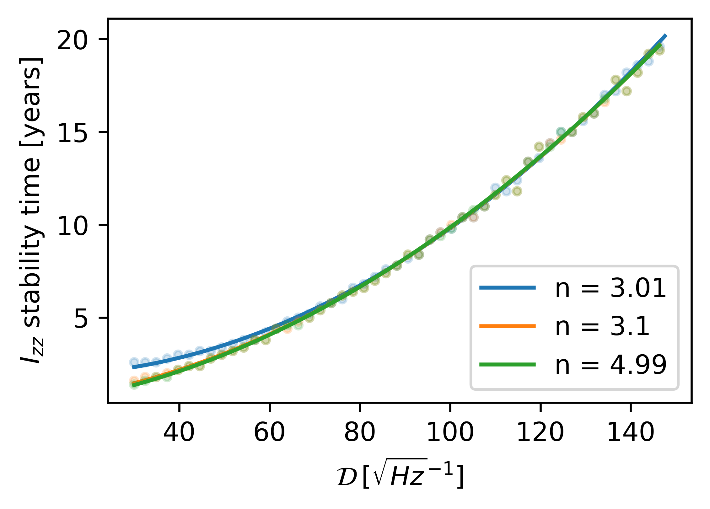
Figure 2: $I_{zz}$ stability time versus sensitivity depth $\mathcal{D}$ for braking indices $n^{\text{in}}=3.01,3.1,4.99$. Here $I_{zz}^{\text{in}}=$2\text{\times}{10}^{38}\text{\,}\mathrm{k}\mathrm{g}\,\mathrm{m}^{2}$$, $f^{\text{in}}=$1000\text{\,}\mathrm{H}\mathrm{z}$$, $\dot{f}^{\text{in}}=$-1\text{\times}{10}^{-9}\text{\,}\mathrm{H}\mathrm{z}\,\mathrm{s}^{-1}$$, and $T=1$ year, with values for $h_{0}$, $\epsilon$, and $m_{p}$ implied by Eqs. (2), (27), and (28) respectively. Plotted are a subsampling of the results from $10^{6}$ samples (light-coloured dots) and best-fit curves (dark-coloured lines).

We define the “stability time” for $I_{zz}$, $\epsilon$, and $m_{p}$ as the time required for the normalised relative errors $\bar{\mathcal{E}}$ of each property to reach $1.1$, i.e. to within 10% of the asymptotic distance error [see Eq. (40)]. Figure 2 plots the stability time for $I_{zz}$ as a function of $n$ and $\mathcal{D}$ for signals with $I_{zz}^{\text{in}}=$2\text{\times}{10}^{38}\text{\,}\mathrm{k}\mathrm{g}\,\mathrm{m}^{2}$$, $f^{\text{in}}=$1000\text{\,}\mathrm{H}\mathrm{z}$$, and $\dot{f}^{\text{in}}=$-1\text{\times}{10}^{-9}\text{\,}\mathrm{H}\mathrm{z}\,\mathrm{s}^{-1}$$. We see that, for continuous wave signals at $\mathcal{D}\sim$30\text{\,}\mathrm{H}\mathrm{z}^{-1/2}$$ initially detected in an all-sky survey, the asymptotic error in $I_{zz}$ is approached after a few years observing with a fully-coherent follow-up search, which would include analysing both archival and future data. For continuous waves detected from known pulsars, where $\mathcal{D}\approx$150\text{\,}\mathrm{H}\mathrm{z}^{-1/2}$$, the asymptotic errors in $I_{zz}$ are not approached until the star is observed for $T\approx$20\text{\,}\mathrm{y}\mathrm{e}\mathrm{a}\mathrm{r}\mathrm{s}$$ which is an unrealistic time span to consider. Note, however, that the definition of “stability time” here assumes the detector sensitivity $S_{h}$ remains constant; in reality $S_{h}$ is likely to decrease over time (Abbott et al., 2020a), particularly if third-generation gravitational wave detectors are constructed (Bailes et al., 2021). Such improvements would decrease the sensitivity depth $\mathcal{D}$ of a detected signal such that the inferred parameters would converge to the asymptotic distance error faster than suggested in figure 2.

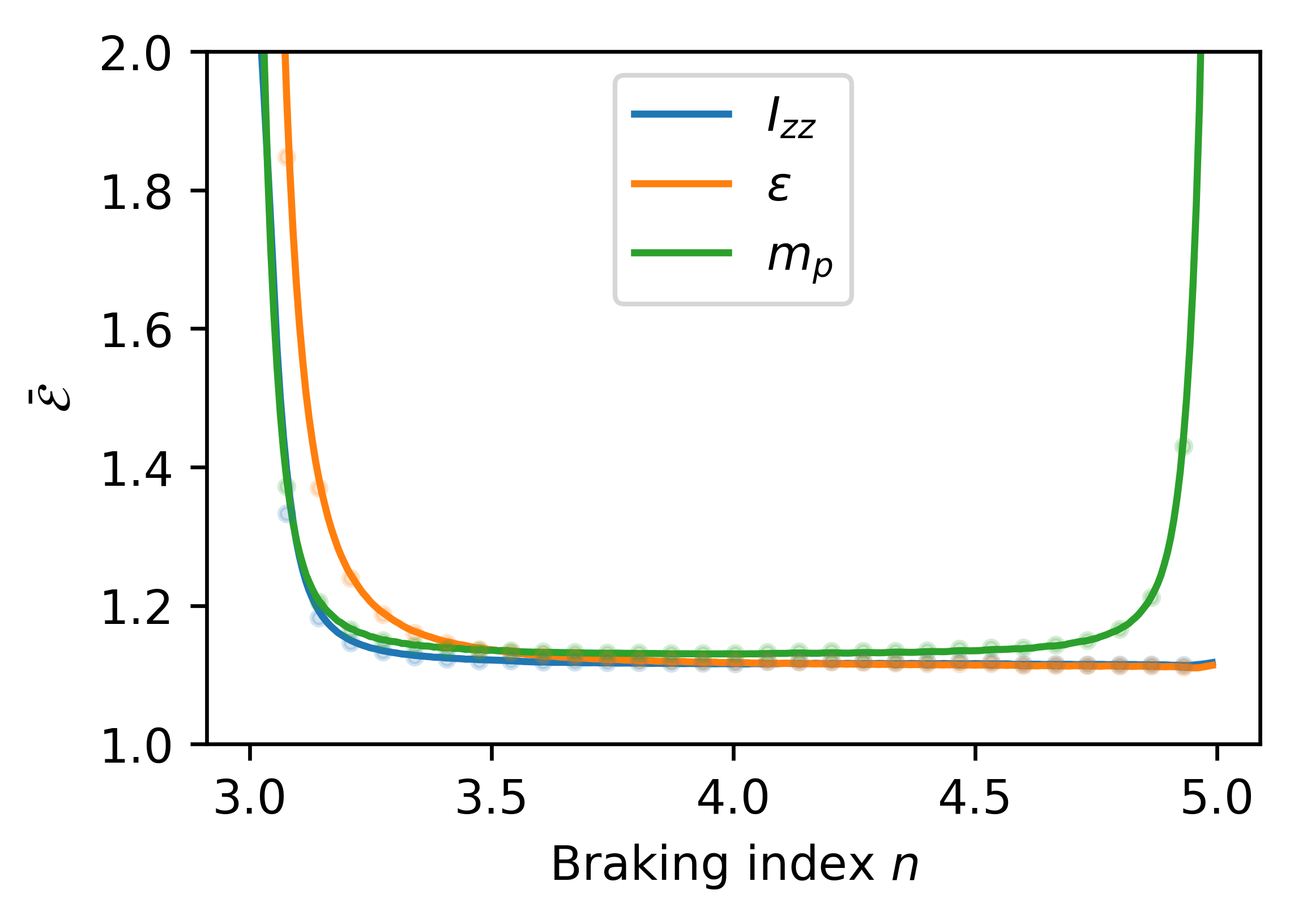
Figure 3: Normalised relative errors ($\bar{\mathcal{E}}$) as a function of braking index $n^{\text{in}}$. Here $I_{zz}^{\text{in}}=$2\text{\times}{10}^{38}\text{\,}\mathrm{k}\mathrm{g}\,\mathrm{m}^{2}$$, $f^{\text{in}}=$1000\text{\,}\mathrm{H}\mathrm{z}$$, $\dot{f}^{\text{in}}=$-1\text{\times}{10}^{-9}\text{\,}\mathrm{H}\mathrm{z}\,\mathrm{s}^{-1}$$, $T=1$ year, and $\mathcal{D}=$30\text{\,}\mathrm{H}\mathrm{z}^{-1/2}$$, with values for $h_{0}$, $\epsilon$, and $m_{p}$ implied by Eqs. (2), (27), and (28) respectively. Plotted are a subsampling of the results from $10^{6}$ samples (light-coloured dots) and best-fit curves (dark-coloured lines).

Figure 3 plots normalised relative errors in $I_{zz}$, $\epsilon$, and $m_{p}$ as functions of $n$ for signals with $I_{zz}^{\text{in}}=$2\text{\times}{10}^{38}\text{\,}\mathrm{k}\mathrm{g}\,\mathrm{m}^{2}$$, $f^{\text{in}}=$1000\text{\,}\mathrm{H}\mathrm{z}$$, $\dot{f}^{\text{in}}=$-1\text{\times}{10}^{-9}\text{\,}\mathrm{H}\mathrm{z}\,\mathrm{s}^{-1}$$, and $\mathcal{D}=$30\text{\,}\mathrm{H}\mathrm{z}^{-1/2}$$. The neutron star properties $I_{zz}$ and $\epsilon$ are best estimated where the star is losing almost all energy in gravitational waves ($n\approx 5$), as expected. On the other hand, the electromagnetic property $m_{p}$ is best estimated where the star is losing its energy through both electromagnetic and gravitational radiation ($n\approx 4$). When energy loss through electromagnetic radiation is more dominant ($n\approx 3$), the errors for all three properties are larger than the $n\approx 4$ case. This is consistent with Eq. (31) - (33) and is because the continuous wave observation cannot measure the spindown parameters accurately when the neutron star only weakly emits continuous waves. However, note that these results are based on the techniques described in section 3. It may be possible for electromagnetic astronomers to use alternate techniques to measure $m_{p}$ with lower errors for neutron stars with certain braking indices.

Figure 4: Normalised relative errors (top to bottom rows) $\bar{\mathcal{E}}(I_{zz})$, $\bar{\mathcal{E}}(\epsilon)$, $\bar{\mathcal{E}}(m_{p})$, for braking indices (left to right columns) $n=3.01$, $3.1$, $4.99$, as functions of $f$ and $\dot{f}$. Plotted are the median errors over $I_{zz}$ and $\xi$, and for $T=1$ year and $\mathcal{D}=$30\text{\,}\mathrm{H}\mathrm{z}^{-1/2}$$. The different colours represent the values of the normalised relative error and the white areas indicate where $\bar{\mathcal{E}}\geq 30.0$ and/or where $3<n^{\text{out}}<5$ no longer holds. A total of $10^{6}$ samples were used in each plot.

Figure 4 plots normalised relative errors $\bar{\mathcal{E}}(I_{zz})$, $\bar{\mathcal{E}}(\epsilon)$, and $\bar{\mathcal{E}}(m_{p})$ as functions of $n$, $f$, and $\dot{f}$, taking the median errors over the sampled ranges of $I_{zz}$ and $\xi$ given in Section 4.1. We assume $T=1$ year and $\mathcal{D}=$30\text{\,}\mathrm{H}\mathrm{z}^{-1/2}$$, which is relevant to a continuous wave signal detected in an all-sky continuous wave survey. The errors in all three neutron star properties are smallest at the highest spin-down rates ($\dot{f}\approx$-{10}^{-8}\text{\,}\mathrm{H}\mathrm{z}\,\mathrm{s}^{-1}$$), where rate of rotational kinetic energy loss from the star is highest, and lowest frequencies ($f\approx$50\text{\,}\mathrm{H}\mathrm{z}$$). Once $|\dot{f}|\lessapprox${10}^{-11}\text{\,}\mathrm{H}\mathrm{z}\,\mathrm{s}^{-1}$$, the errors are sufficiently large that $n$ cannot be reliably measured, the restriction $3<n^{\text{out}}<5$ is no longer satisfied, and most Monte Carlo samples must be discarded (see Section 4.2). For each heatmap, the error as a function of $|\dot{f}|$ increases more rapidly for lower $f$ than for higher $f$, consistent with the $f^{-2}$ dependence of the $T^{-3}$ terms in Eqs. (31) – (33).

Figure 4 suggests that normalised relative errors $\bar{\mathcal{E}}\lesssim 1.2$ are achievable over much of the $f$–$\dot{f}$ parameter space typically searched over for continuous waves, and particularly for rapidly spinning-down sources ($|\dot{f}|\gtrapprox${10}^{-9}\text{\,}\mathrm{H}\mathrm{z}\,\mathrm{s}^{-1}$$). This implies errors in $I_{zz}$ of $\sim 32\%$, and errors in $\epsilon$ and $m_{p}$ of $\sim 16\%$. Given that models of non-axisymmetrically deformed neutron stars (Bonazzola & Gourgoulhon, 1996; Ushomirsky et al., 2000; Cutler, 2002; Owen, 2005; Payne & Melatos, 2006; Haskell et al., 2008; Vigelius & Melatos, 2009; Wette et al., 2010; Priymak et al., 2011) typically predict $\epsilon$ only to an order of magnitude, the error in $\epsilon$ should be sufficient to test such models. A $\sim 30\%$ error in $I_{zz}$ is of similar magnitude to measurements of $I_{zz}$ for PSR J0737$-$3039A. Miao et al. (2022) found errors of $\sim 10$ – $20\%$ after assuming an equation of state; without that assumption the errors in $I_{zz}$ increase by a factor of $\sim 4$. In comparison, no explicit assumptions regarding the neutron star equation of state are required for the framework of Section 3 or the results presented in Section 5. Estimates of $m_{p}$ using this framework could also be compared to those estimates for known pulsars and serve as an independent verification of such measurements.

Pulsar	Crab (J0534+2200)	Vela (J0835-4510)
$f_{\text{GW}}$ ($\mathrm{H}\mathrm{z}$)	59.2	22.4
$\dot{f}_{\text{GW}}$ ($\mathrm{H}\mathrm{z}\,\mathrm{s}^{-1}$)	$-7.4\text{\times}{10}^{-10}$	$-5.6\text{\times}{10}^{-11}$
$r$ ($\mathrm{k}\mathrm{p}\mathrm{c}$)	2.0	0.157
$\Delta r/r$	0.25	0.066
$h_{0}^{95\%}$	$1.5\text{\times}{10}^{-26}$	$2.2\text{\times}{10}^{-25}$

Table 1: Properties of two young pulsars. Here $h_{0}^{95\%}$ is the 95% confidence level upper limits on the gravitational wave amplitude measured by Abbott et al. (2020c). Adapted from Abbott et al. (2020c).

Pulsar	Crab (J0534+2200)	Vela (J0835-4510)
$n^{\text{max}}$	3.0025	3.0050
$\mathcal{E}(I_{zz})$	0.97	0.99
$\mathcal{E}(\epsilon)$	29	93
$\mathcal{E}(m_{p})$	0.82	0.91

Table 2: Maximum braking index ($n^{\text{max}}$) and relative errors ($\mathcal{E}$) for two young pulsars. Here $n^{\text{max}}$ is computed by rearranging Eq. 26 and substituting in the known $f$ and $\dot{f}$, measured $h_{0}^{95\%}$, and assuming $I_{zz}=$1\text{\times}{10}^{38}\text{\,}\mathrm{k}\mathrm{g}\,\mathrm{m}^{2}$$ (which is consistent with Abbott et al. 2020c). The relative errors are computed for $T=1$ year, $\mathcal{D}=$150\text{\,}\mathrm{H}\mathrm{z}^{-1/2}$$, and for $10^{6}$ samples.

Table 1 shows the properties of two young pulsars. By rearranging Eq. 26 for $n$, it is possible to compute the maximum braking indices ($n^{\text{max}}$) consistent with the observational upper limits $h_{0}^{95\%}$. This is computed in Table 2, where it is necessary to assume $I_{zz}=$1\text{\times}{10}^{38}\text{\,}\mathrm{k}\mathrm{g}\,\mathrm{m}^{2}$$ which is consistent with Abbott et al. 2020c. If continuous waves from the two pulsars were observed with $n=n^{\text{max}}$, Table 2 also shows the relative errors of the parameters that would be inferred. These relative errors are larger than those in Figure 4 because of the extremely low braking indices and increased sensitivity depths for continuous waves from known pulsars. Nevertheless, this shows how continuous waves could infer properties of known pulsars that are otherwise difficult to measure.

6 Assumptions

This section elaborates on some of the assumptions made in this paper.

We assume that continuous waves will eventually be detectable by contemporary and/or future gravitational wave detectors. This remains uncertain. The lowest bounds on $\epsilon\propto 10^{-11}$ from magnetic field distortions (Bonazzola & Gourgoulhon, 1996) are small enough that only a few detections, at best, may be expected in the next generation of detectors (Pitkin, 2011). Stars with stronger magnetic fields ($B\sim 10^{15}$ Gauss) lead to larger ellipticities $\epsilon\gtrsim 10^{-6}$ (Cutler, 2002; Haskell et al., 2008) which are more likely detectable by the current generation of gravitational wave detectors. It is also possible that the internal magnetic fields of neutron stars could be stronger than their surface fields (Lasky, 2015; Bransgrove et al., 2017). For known pulsars, only a small fraction are likely to be detectable, particularly if the fraction of rotational kinetic energy emitted in gravitational waves is small (Pitkin, 2011). That said, the $\mathcal{O}(10^{3})$ known pulsars may not be representative of the $\mathcal{O}(10^{8})$ population of galactic neutron stars (Palomba, 2005; Knispel & Allen, 2008; Wade et al., 2012; Cieślar et al., 2021; Reed et al., 2021), which could include a sub-population of strong gravitational wave emitters or “gravitars”.

We assume that Eq. (19) is a reasonable starting point for modelling the energy radiated by neutron stars. It is generally assumed that electromagnetic radiation from known pulsars is predominately dipolar, that neutron stars are triaxial rotors, and that continuous wave radiation would be predominately quadrupolar (Ostriker & Gunn, 1969). Recent measurements of hot surface regions of several neutron stars using NICER provide evidence for non-dipolar magnetic fields in millisecond pulsars (Bilous et al., 2019; Riley et al., 2019, 2021). However, alternate models with multipolar magnetic fields are not well understood (Gralla et al., 2017; Lockhart et al., 2019; Riley et al., 2019) and their formation during stellar evolution is also unclear (Mitchell et al., 2015; Gourgouliatos & Hollerbach, 2017). While dipolar magnetic fields are a reasonable starting point for this analysis, future work could extend the framework developed here to more complex magnetic field configurations.

The energy emission assumptions of Eq. (19) predicts $3<n<5$, which is at odds with measured braking indices from radio pulsars which span orders of magnitude outside this range (Johnston & Galloway, 1999; Zhang & Xie, 2012; Lower et al., 2021). Modified models for pulsar emission have been proposed to explain the observed braking indices (Allen & Horvath, 1997; Melatos, 1997; Xu & Qiao, 2001; Alvarez & Carrami nana, 2004; Yue et al., 2007; Hamil et al., 2015) including the addition of gravitational waves (de Araujo et al., 2016; Chishtie et al., 2018). On the other hand, accurate phase-connected measurement of a second time derivative of the rotation frequency needed to compute $n$ is challenging (cf. Johnston & Galloway, 1999). Existing measurements of $n$ are generally dominated by timing noise (Hobbs et al., 2004; Hobbs et al., 2010), with some possible exceptions (Archibald et al., 2016; Lasky et al., 2017).

Prospects for an accurate determination of $n$ may be improved by a continuous wave detection. Since gravitational wave detectors are omni-directional, gravitational wave data is recorded at a much higher duty cycle ($\gtrsim 70\%$; Abbott et al. 2020a) than typical pulsar observing cadences (e.g. $\lesssim 35\text{hours/year}\sim 0.4\%$; Lam 2018). Although $\ddot{f}$ would not be resolved in all-sky continuous wave surveys, which sacrifice phase resolution in favour of reduced computational cost, a candidate from such a survey would then be followed up using a fully phase-coherent search in a restricted parameter space around the candidate. Such a search would be computationally inexpensive, and would be able to resolve $\ddot{f}$ to a resolution $\sim\mathcal{D}/T^{7/2}$ [cf. Eq. (14)].

Pulse emission from radio pulsars is subject to various noise sources (de Kool & Anzer, 1993; Archibald et al., 2008; Lentati et al., 2016; Goncharov et al., 2021). Individual pulses from radio pulsars are highly variable, and achieve a stable pulse profile once averaged over many cycles (Kramer, 2005). It remains to be seen whether detected continuous wave signals will suffer from comparable noise sources (Ashton et al., 2015; Suvorova et al., 2016; Meyers et al., 2021a, b). Gravitational waves, being weakly interacting, are not perturbed by matter along the line of sight to the star, unless the signal is lensed (Biesiada & Harikumar, 2021). Furthermore, unlike electromagnetic emission that arises from the outer surface and plasma of the star, where a small fraction of the neutron star mass is located, gravitational wave emission arises from the rotating mass quadrupole. Physical processes within the star would need considerable energy to perturb the star’s rotation, and hence the continuous wave signal, in order to achieve a level of noisiness comparable to timing noise observed in radio pulsars. Superfluid vortices within the star’s interior are suspected of being responsible for glitches (van Eysden & Melatos, 2008; Warszawski & Melatos, 2011; Ho et al., 2015; Haskell et al., 2020; Abbott et al., 2021f) which do perturb the star’s rotation and may affect the detectability of continuous waves (Ashton et al., 2018). Glitches, however, are observed as discrete events even in prolifically glitchy pulsars (Ho et al., 2020) and the extent to which they could constitute a persistent noise source in detected continuous wave signals is unknown (Yim & Jones, 2022). Should continuous waves measure a braking index from $n\notin[3,5]$, this might represent stronger evidence for new physics than current radio pulsar observations.

Finally, we assume that the neutron star also emits electromagnetic radiation, and that a measurement of its distance can be obtained. Neutron stars are expected to possess magnetic fields (Reisenegger, 2001) and will therefore (provided that the field is not symmetric about the star’s rotation axis) emit electromagnetic radiation. Continuous waves may first be detected either from a known pulsar, or as a gravitational-wave-only candidate from an all-sky survey; in either case, observations over $T\gtrsim 1$ year would give the sky position of the source to sub-arcsecond resolution (Riles, 2013, 2017). This would facilitate further electromagnetic observations to either detect an electromagnetic counterpart, or else refine the properties of one already known. Other methods exist to measure stellar distances in the absence of a radio pulsar detection; parallax may be used to determine the distances to nearby neutron stars (Seto, 2005; Walter et al., 2010), while distances to neutron stars in supernova remnants may be inferred through observation of the radial velocities of the surrounding ejecta (Reed et al., 1995). These methods yield comparable uncertainties to radio pulsar distances.

7 Summary

This paper presents a first analysis of what properties may be inferred from a neutron star radiating both electromagnetic and detectable continuous gravitational waves. We develop a simple Fisher information-based parameter estimation framework, which gives estimates of the uncertainties for the stellar moment of inertia $I_{zz}$, equatorial ellipticity $\epsilon$, and component of the magnetic dipole moment perpendicular to its rotation axis $m_{p}$. This framework does not assume a particular neutron star equation of state and only requires a detection of continuous waves and a measurable distance to the star.

Monte Carlo simulations over a parameter space of gravitational wave frequency and its derivatives, typical of that covered by all-sky continuous wave surveys, demonstrate that the relative errors in $I_{zz}$, $\epsilon$, and $m_{p}$ asymptote to 14–27%, assuming a 20% error in distance. The observation time required to reach these limits may be as little as a few years for a strong continuous wave signal detected in an all-sky survey; for weaker signals, such as those potentially associated with known pulsars, longer observations may be required. We also find that the errors of the inferred parameters tend to be smaller when the braking index is close to $n\approx 4$, when $f$ is smaller and when $|\dot{f}|$ is larger.

Future work could extend the assumed neutron star energy loss model of Eq. (19) to include a more complex model of the neutron star magnetic field, e.g. Lasky & Melatos (2013). Recasting the parameter inference in a Bayesian framework would also be advantageous as it would avoid the coordinate singularities present in the Fisher matrix approach and make use of prior information from other gravitational wave and electromagnetic observations of neutron stars.

Data Availability

The data underlying this article will be shared on reasonable request to the corresponding author(s).

References

- Aasi et al. (2015) Aasi J., et al., 2015, Class. Quantum Gravity, 32, 074001
- Abbott et al. (2016) Abbott B. P., et al., 2016, Phys. Rev. Lett., 116, 061102
- Abbott et al. (2017a) Abbott B. P., et al., 2017a, Phys. Rev. Lett., 119, 161101
- Abbott et al. (2017b) Abbott B. P., et al., 2017b, ApJ, 848, L13
- Abbott et al. (2020a) Abbott B. P., et al., 2020a, Living Rev. Relativ., 23, 3
- Abbott et al. (2020b) Abbott R., et al., 2020b, ApJ, 902, L21
- Abbott et al. (2020c) Abbott R., et al., 2020c, ApJ, 902, L21
- Abbott et al. (2021a) Abbott R., et al., 2021a, Phys. Rev. X, 11, 021053
- Abbott et al. (2021b) Abbott R., et al., 2021b, Phys. Rev. D, 103, 064017
- Abbott et al. (2021c) Abbott R., et al., 2021c, Phys. Rev. D, 104, 082004
- Abbott et al. (2021d) Abbott R., et al., 2021d, ApJ, 913, L27
- Abbott et al. (2021e) Abbott R., et al., 2021e, ApJ, 921, 80
- Abbott et al. (2021f) Abbott R., et al., 2021f, ApJ, 922, 71
- Abbott et al. (2022a) Abbott R., et al., 2022a, Phys. Rev. D, 105, 022002
- Abbott et al. (2022b) Abbott R., et al., 2022b, Phys. Rev. D, 105, 102001
- Abbott et al. (2022c) Abbott R., et al., 2022c, Phys. Rev. D, 105, 082005
- Abbott et al. (2022d) Abbott R., et al., 2022d, ApJ, 932, 133
- Abbott et al. (2022e) Abbott R., et al., 2022e, ApJ, 935, 1
- Acernese et al. (2015) Acernese F., et al., 2015, Class. Quantum Gravity, 32, 024001
- Akutsu et al. (2019) Akutsu T., et al., 2019, Nature Astronomy, 3, 35
- Akutsu et al. (2020) Akutsu T., et al., 2020, Prog. Theor. Exp. Phys., 2021
- Allen & Horvath (1997) Allen M. P., Horvath J. E., 1997, ApJ, 488, 409
- Alvarez & Carrami nana (2004) Alvarez C., Carrami nana A., 2004, A&A, 414, 651
- Andersson (1998) Andersson N., 1998, ApJ, 502, 708
- Archibald et al. (2008) Archibald A. M., Dib R., Livingstone M. A., Kaspi V. M., 2008, in Bassa C., Wang Z., Cumming A., Kaspi V. M., eds, Am. Inst. Phys. Conf. Ser. Vol. 983, 40 Years of Pulsars: Millisecond Pulsars, Magnetars and More. pp 265–267 (arXiv:0712.3322), doi:10.1063/1.2900158
- Archibald et al. (2016) Archibald R. F., et al., 2016, ApJ, 819, L16
- Ashton et al. (2015) Ashton G., Jones D. I., Prix R., 2015, Phys. Rev. D, 91, 062009
- Ashton et al. (2018) Ashton G., Prix R., Jones D. I., 2018, Phys. Rev. D, 98, 063011
- Bailes et al. (2021) Bailes M., et al., 2021, Nat. Rev. Phys., 3, 344
- Balasubramanian et al. (1996) Balasubramanian R., Sathyaprakash B. S., Dhurandhar S. V., 1996, Phys. Rev. D, 53, 3033
- Behnke et al. (2015) Behnke B., Papa M. A., Prix R., 2015, Phys. Rev. D, 91, 064007
- Bejger et al. (2005) Bejger M., Bulik T., Haensel P., 2005, MNRAS, 364, 635
- Benke et al. (2018) Benke K. K., Norng S., Robinson N. J., Benke L. R., Peterson T. J., 2018, Stoch. Environ. Res. Risk Assess., 32, 2971
- Biesiada & Harikumar (2021) Biesiada M., Harikumar S., 2021, Universe, 7, 502
- Bilous et al. (2019) Bilous A. V., et al., 2019, The Astrophysical Journal Letters, 887, L23
- Blanchet et al. (2001) Blanchet L., Kopeikin S., Schäfer G., 2001, in Lämmerzahl C., Everitt C. W. F., Hehl F. W., eds, Gyros, Clocks, Interferometers…: Testing Relativistic Graviy in Space. Springer Berlin Heidelberg, Berlin, Heidelberg, pp 141–166
- Bonazzola & Gourgoulhon (1996) Bonazzola S., Gourgoulhon E., 1996, A&A, 312, 675
- Brady et al. (1998) Brady P. R., Creighton T., Cutler C., Schutz B. F., 1998, Phys. Rev. D, 57, 2101
- Bransgrove et al. (2017) Bransgrove A., Levin Y., Beloborodov A., 2017, MNRAS, 473, 2771
- Chishtie et al. (2018) Chishtie F. A., Zhang X., Valluri S. R., 2018, Class. Quantum Gravity, 35, 145012
- Cieślar et al. (2021) Cieślar M., Bulik T., Curyło M., Sieniawska M., Singh N., Bejger M., 2021, A&A, 649, 1
- Condon & Ransom (2016) Condon J. J., Ransom S. M., 2016, Essential Radio Astronomy. Princeton University Press, Princeton, pp 208–232, http://www.jstor.org/stable/j.ctv5vdcww.10
- Covas et al. (2022) Covas P. B., Papa M. A., Prix R., Owen B. J., 2022, ApJ, 929, L19
- Cutler (2002) Cutler C., 2002, Phys. Rev. D, 66, 084025
- Damour & Schäeer (1988) Damour T., Schäeer G., 1988, Nuovo Cimento B, 101, 127
- Dreissigacker et al. (2018) Dreissigacker C., Prix R., Wette K., 2018, Phys. Rev. D, 98, 084058
- Dupuis & Woan (2005) Dupuis R. J., Woan G., 2005, Phys. Rev. D, 72, 102002
- Goncharov et al. (2021) Goncharov B., et al., 2021, MNRAS, 502, 478
- Gourgouliatos & Hollerbach (2017) Gourgouliatos K. N., Hollerbach R., 2017, ApJ, 852, 21
- Gralla et al. (2017) Gralla S. E., Lupsasca A., Philippov A., 2017, ApJ, 851, 137
- Hamil et al. (2015) Hamil O., Stone J. R., Urbanec M., Urbancová G., 2015, Phys. Rev. D, 91, 063007
- Haskell et al. (2008) Haskell B., Samuelsson L., Glampedakis K., Andersson N., 2008, MNRAS, 385, 531
- Haskell et al. (2020) Haskell B., Antonopoulou D., Barenghi C., 2020, MNRAS, 499, 161
- Ho et al. (2015) Ho W. C. G., Espinoza C. M., Antonopoulou D., Andersson N., 2015, Sci. Adv., 1, e1500578
- Ho et al. (2020) Ho W. C. G., et al., 2020, MNRAS, 498, 4605
- Hobbs et al. (2004) Hobbs G., Lyne A. G., Kramer M., Martin C. E., Jordan C., 2004, MNRAS, 353, 1311
- Hobbs et al. (2010) Hobbs G., Lyne A. G., Kramer M., 2010, MNRAS, 402, 1027
- Jaranowski & Królak (1999) Jaranowski P., Królak A., 1999, Phys. Rev. D, 59
- Jaranowski et al. (1998) Jaranowski P., Krolak A., Schutz B., 1998, Phys. Rev. D, 58
- Johnston & Galloway (1999) Johnston S., Galloway D., 1999, MNRAS, 306, L50
- Knispel & Allen (2008) Knispel B., Allen B., 2008, Phys. Rev. D, 78, 1
- Kramer (2005) Kramer M., 2005, in Gurvits L. I., Frey S., Rawlings S., eds, EAS Publications Series Vol. 15, EAS Publications Series. p. 219, doi:10.1051/eas:2005155
- Kramer et al. (2021) Kramer M., et al., 2021, Phys. Rev. X, 11, 041050
- Lam (2018) Lam M. T., 2018, ApJ, 868, 33
- Lasky (2015) Lasky P. D., 2015, Publ. Astron. Soc. Australia, 32, e034
- Lasky & Melatos (2013) Lasky P. D., Melatos A., 2013, Phys. Rev. D, 88, 103005
- Lasky et al. (2017) Lasky P. D., Leris C., Rowlinson A., Glampedakis K., 2017, ApJ, 843, L1
- Lentati et al. (2016) Lentati L., et al., 2016, MNRAS, 458, 2161
- Lindblom et al. (1998) Lindblom L., Owen B. J., Morsink S. M., 1998, Phys. Rev. Lett., 80, 4843
- Lockhart et al. (2019) Lockhart W., Gralla S. E., Özel F., Psaltis D., 2019, Monthly Notices of the Royal Astronomical Society, 490, 1774
- Lower et al. (2021) Lower M. E., et al., 2021, MNRAS, 508, 3251
- Manchester et al. (1985) Manchester R. N., Newton L. M., Durdin J. M., 1985, Nature, 313, 374
- Melatos (1997) Melatos A., 1997, MNRAS, 288, 1049
- Melatos & Payne (2005) Melatos A., Payne D. J. B., 2005, ApJ, 623, 1044
- Meyers et al. (2021a) Meyers P. M., Melatos A., O’Neill N. J., 2021a, MNRAS, 502, 3113
- Meyers et al. (2021b) Meyers P. M., O’Neill N. J., Melatos A., Evans R. J., 2021b, MNRAS, 506, 3349
- Miao et al. (2022) Miao Z., Li A., Dai Z.-G., 2022, MNRAS, 515, 5071
- Miller et al. (2019) Miller M. C., et al., 2019, ApJ, 887, L24
- Mitchell et al. (2015) Mitchell J. P., Braithwaite J., Reisenegger A., Spruit H., Valdivia J. A., Langer N., 2015, Monthly Notices of the Royal Astronomical Society, 447, 1213
- Mølnvik & Østgaard (1985) Mølnvik T., Østgaard E., 1985, Nucl. Phys. A, 437, 239
- Ostriker & Gunn (1969) Ostriker J. P., Gunn J. E., 1969, ApJ, 157, 1395
- Owen (1996) Owen B. J., 1996, Phys. Rev. D, 53, 6749
- Owen (2005) Owen B. J., 2005, Phys. Rev. Lett., 95, 211101
- Palomba (2005) Palomba C., 2005, MNRAS, 359, 1150
- Payne & Melatos (2006) Payne D. J. B., Melatos A., 2006, ApJ, 641, 471
- Pitkin (2011) Pitkin M., 2011, MNRAS, 415, 1849
- Pitkin et al. (2017) Pitkin M., Isi M., Veitch J., Woan G., 2017, arXiv
- Prix (2007) Prix R., 2007, Phys. Rev. D, 75, 023004
- Prix (2011) Prix R., 2011, Technical Report T0900149-v6, The F-statistic and its implementation in ComputeFStatistic_v2. LIGO, https://dcc.ligo.org/T0900149/public
- Priymak et al. (2011) Priymak M., Melatos A., Payne D. J. B., 2011, MNRAS, 417, 2696
- Reed et al. (1995) Reed J. E., Hester J. J., Fabian A. C., Winkler P. F., 1995, ApJ, 440, 706
- Reed et al. (2021) Reed B. T., Deibel A., Horowitz C. J., 2021, ApJ, 921, 89
- Reisenegger (2001) Reisenegger A., 2001, in Mathys G., Solanki S. K., Wickramasinghe D. T., eds, Astronomical Society of the Pacific Conference Series Vol. 248, Magnetic Fields Across the Hertzsprung-Russell Diagram. p. 469 (arXiv:astro-ph/0103010)
- Riles (2013) Riles K., 2013, Prog. Part. Nucl. Phys., 68, 1
- Riles (2017) Riles K., 2017, Mod. Phys. Lett. A, 32
- Riley et al. (2019) Riley T. E., et al., 2019, The Astrophysical Journal Letters, 887, L21
- Riley et al. (2021) Riley T. E., et al., 2021, The Astrophysical Journal Letters, 918, L27
- Seto (2005) Seto N., 2005, Phys. Rev. D, 71, 123002
- Sieniawska & Jones (2022) Sieniawska M., Jones D. I., 2022, MNRAS, 509, 5179
- Smits et al. (2011) Smits R., Tingay S. J., Wex N., Kramer M., Stappers B., 2011, A&A, 528, A108
- Steiner et al. (2015) Steiner A. W., Gandolfi S., Fattoyev F. J., Newton W. G., 2015, Phys. Rev. C, 91, 015804
- Suvorova et al. (2016) Suvorova S., Sun L., Melatos A., Moran W., Evans R. J., 2016, Phys. Rev. D, 93, 123009
- Taylor & Cordes (1993) Taylor J., Cordes J., 1993, ApJ, 411, 674
- Tenorio et al. (2021) Tenorio R., Keitel D., Sintes A. M., 2021, Universe, 7, 474
- Ushomirsky et al. (2000) Ushomirsky G., Cutler C., Bildsten L., 2000, MNRAS, 319, 902
- Vallisneri (2008) Vallisneri M., 2008, Phys. Rev. D, 77, 042001
- Van Den Broeck (2005) Van Den Broeck C., 2005, Class. Quantum Gravity, 22, 1825
- Verbiest et al. (2012) Verbiest J. P. W., Weisberg J. M., Chael A. A., Lee K. J., Lorimer D. R., 2012, ApJ, 775
- Vigelius & Melatos (2009) Vigelius M., Melatos A., 2009, MNRAS, 395, 1972
- Wade et al. (2012) Wade L., Siemens X., Kaplan D. L., Knispel B., Allen B., 2012, Phys. Rev. D, 86, 1
- Walter et al. (2010) Walter F. M., Eisenbeiß T., Lattimer J. M., Kim B., Hambaryan V., Neuhäuser R., 2010, ApJ, 724, 669
- Warszawski & Melatos (2011) Warszawski L., Melatos A., 2011, MNRAS, 415, 1611
- Wette et al. (2008) Wette K., et al., 2008, Class. Quantum Gravity, 25, 235011
- Wette et al. (2010) Wette K., Vigelius M., Melatos A., 2010, MNRAS, 402, 1099
- Worley et al. (2008) Worley A., Krastev P. G., Li B.-A., 2008, ApJ, 685, 390
- Xu & Qiao (2001) Xu R. X., Qiao G. J., 2001, ApJ, 561, L85
- Yao et al. (2017) Yao J. M., Manchester R. N., Wang N., 2017, ApJ, 835
- Yim & Jones (2022) Yim G., Jones D. I., 2022, arXiv e-prints, p. arXiv:2204.12869
- Yue et al. (2007) Yue Y. L., Xu R. X., Zhu W. W., 2007, Adv. Space Res., 40, 1491
- Zhang & Xie (2012) Zhang S.-N., Xie Y., 2012, ApJ, 761, 102
- Zimmermann & Szedenits (1979) Zimmermann M., Szedenits Jr. E., 1979, Phys. Rev. D, 20, 351
- de Araujo et al. (2016) de Araujo J. C. N., Coelho J. G., Costa C. A., 2016, Eur. Phys. J. C, 76, 481
- de Kool & Anzer (1993) de Kool M., Anzer U., 1993, MNRAS, 262, 726
- van Eysden & Melatos (2008) van Eysden C. A., Melatos A., 2008, Class. Quantum Gravity, 25, 225020