2022
[1]\fnmKeith \surBurghardt
[1]\orgnameUSC Information Sciences Institute, \orgaddress\street4676 Admiralty Way, \cityMarina del Rey, \postcode90292, \stateCA, \countryUSA 2]\orgdivInstitute of Behavioral Science, \orgnameUniversity of Colorado Boulder, \orgaddress\street483 UCB, \cityBoulder, \postcode80309, \stateCO, \countryUSA 3]\orgdivCooperative Institute for Research in Environmental Sciences (CIRES), \orgnameUniversity of Colorado Boulder, \orgaddress\street216 UCB, \cityBoulder, \postcode80309, \stateCO, \countryUSA 4]\orgdivDepartment of Geography, \orgnameUniversity of Colorado Boulder, \orgaddress\street260 UCB, \cityBoulder, \postcode80309, \stateCO, \countryUSA
Analyzing urban scaling laws in the United States over 115 years
Abstract
The scaling relations between city attributes and population are emergent and ubiquitous aspects of urban growth. Quantifying these relations and understanding their theoretical foundation, however, is difficult due to the challenge of defining city boundaries and a lack of historical data to study city dynamics over time and space. To address this issue, we analyze scaling between city infrastructure and population across 857 United States metropolitan areas over an unprecedented 115 years using dasymetrically refined historical population estimates, historical urban road network models, and multi-temporal settlement data to define dynamic city boundaries based on settlement density. We demonstrate the clearest evidence that urban scaling exponents can closely match theoretical models over a century if cities are defined as dense settlement patches. Despite the close quantitative agreement with theory, the empirical scaling relations unexpectedly vary across regions. Our analysis of scaling coefficients, meanwhile, reveals that a city in 2015 uses more developed land and kilometers of road than a city with a similar population in 1900, which has serious implications for urban development and impacts on the local environment. Overall, our results offer a new way to study urban systems based on novel, geohistorical data.
keywords:
Urban scaling, temporal analysis, cross-sectional analysis, urbanization, allometric analysis, historical settlement modelling, geospatial data integrationCities are expanding at an unprecedented pace, with the majority of the world’s population now living in urban environments of Economic \BBA Social Affairs (\APACyear2019), and a near-majority in each continent Montgomery (\APACyear2008). Cities encompass highly diverse geographies and populations, both in size and composition, yet seemingly robust urban patterns emerge from this complexity Zipf (\APACyear1949); Jiang \BOthers. (\APACyear2015); Eeckhout (\APACyear2004); Jiang \BBA Jia (\APACyear2011); Rozenfeld \BOthers. (\APACyear2008, \APACyear2011); Gabaix \BBA Ioannides (\APACyear2004); Batty (\APACyear2006); Jusup \BOthers. (\APACyear2022); J.e.a. Lobo (\APACyear2020); Reia \BOthers. (\APACyear2022). These patterns are important not only because of the significance of cities and because they provide a uniform reference frame for comparing cities, but also because they offer a framework to understand emergent phenomena in complex systems. Among the most widely studied examples of urban patterns are scaling relations between features of a city and its population size Bettencourt \BOthers. (\APACyear2007); Bettencourt (\APACyear2013); Jusup \BOthers. (\APACyear2022), of the form
| (1) |
where is the city population, is the scaling coefficient, and is the scaling exponent. We define the constant to be such that a log-log plot will have the relation . The universality of these patterns has recently been called into question, however, because the scaling exponents appear to vary over time Batty (\APACyear2006); Louf \BBA Barthelemy (\APACyear2014); Bettencourt \BOthers. (\APACyear2020); Keuschnigg (\APACyear2019); Depersin \BBA Barthelemy (\APACyear2018). In this paper, we analyze the scaling of cities in the conterminous United States (CONUS) over more than a century, from 1900–2015, in order to understand changes in scaling exponents and coefficients over a time period that is longer than in any previous study Bettencourt \BOthers. (\APACyear2020); Keuschnigg (\APACyear2019); Depersin \BBA Barthelemy (\APACyear2018). We define cities based on settlement densities to capture the evolution of city boundaries over time. We use dasymetric refinement Maantay \BOthers. (\APACyear2007); Wei \BOthers. (\APACyear2017); Huang \BOthers. (\APACyear2021) to determine populations within built-up areas. We then utilize novel techniques to capture the developed area, indoor area, building footprint area, and kilometers of roads within these city “patches.” By capturing scaling over the span of decades, we better understand how urban environments and infrastructure have developed in relationship to their population. Surprisingly, we find that scaling law exponents are stable over time, in contrast to recent research Depersin \BBA Barthelemy (\APACyear2018); Keuschnigg (\APACyear2019), while scaling law coefficients increase dramatically over time, which implies that a city in 2015 far less dense and contains larger houses than a city with a similar population in 1900. Overall, our work provides new insights into the persistence of urban patterns, while revealing how different geographies, as defined by e.g., topography, may nonetheless impact scaling relations. This adds nuance to theoretical arguments behind and implications of urban scaling Bettencourt (\APACyear2013).
Results
We recently developed an approach and data infrastructure to measure the long term evolution of settlements Leyk \BBA Uhl (\APACyear2018\APACexlab\BCnt1) and road networks for 850 cities within the US since 1900 Burghardt \BOthers. (\APACyear2022), which adds to the growing literature on reconstructing land use over time Li \BOthers. (\APACyear2022); El Gouj \BOthers. (\APACyear2022). We apply these data to reconstruct the infrastructure of cities as they grow, as shown in Fig. 1. We treat cities as areas with dense built up settlements that can span large parts of Core-Based Statistical Areas (CBSAs), as shown in Fig. 1a–c for 1900–2015.

We calculate city features, namely their total developed area, indoor area, building footprint area, road length, and population size (see Materials and Methods for details). Developed area is the land area of developments (yellow area in Fig. 1d), while building footprint area is the acreage of all buildings within a city boundary (Fig. 1e). Indoor area (Fig. 1f) meanwhile represents the total building floorspace across all floors rather than the footprint acreage. Road length is defined as the total kilometers of road found within each city boundary (Fig. 1g). We see more examples of built-up areas in Fig. 2 for Atlanta, Georgia; San Francisco, California; Denver, Colorado; Los Angeles, California; San Antonio, Texas; El Paso, Texas; and Casper, Wyoming, demonstrating how the developed area spreads from a central location outwards over time.

We then reconstruct historical city populations using gridded HISDAC-US building data Leyk \BBA Uhl (\APACyear2018\APACexlab\BCnt1) and historical US Census CBSA populations U.C. Bureau (\APACyear2020\APACexlab\BCnt3, \APACyear2020\APACexlab\BCnt1, \APACyear2020\APACexlab\BCnt2). In many areas of the US, we only know historical populations down to the county-level, therefore to infer populations within arbitrarily defined city boundaries, we find the fraction of settlements within a CBSA that are within the city boundaries and multiply this fraction by the CBSA population that year. The logic behind this methodology is that we observe a strong correlation between the number of buildings and population within a given county (Supplementary Figure S1), therefore the proportional of houses within a city is a good indication of its historical population. We confirm the accuracy of this method in Supplementary Figure S2 where we compare our population estimation method to alternative methods Huang \BOthers. (\APACyear2021); Baynes \BOthers. (\APACyear2022). The city boundaries we define are based on built-up intensity, which is similar to those based on population density Arcaute \BOthers. (\APACyear2015), or other metrics Jia \BBA Jiang (\APACyear2010); Jiang \BBA Miao (\APACyear2015); Jiang \BBA Jia (\APACyear2011). While there are a number of other ways to define cities Cottineau \BOthers. (\APACyear2017); Parr (\APACyear2007); Small \BOthers. (\APACyear2005), including those based on workforce and consumption, we use the current method because it is a reasonable proxy of these alternative definitions (people often travel near their home González \BOthers. (\APACyear2008), making area around a settlement location a good proxy of where people travel and commute). Moreover, our definition is robust enough that we can uncover city boundaries far back in time.
Scaling over time


We show scaling relations in Fig. 3, in which the slope (scaling exponent) of each scaling relation is relatively stable, while the y-intercept of the scaling relations (scaling coefficient) tends to increase over time. We quantify these findings as shown for scaling exponents in Fig. 4 and scaling coefficients in Fig. 5. These results are robust to variations in data quality, as shown in Supplementary Figures S3 & S4. Cities produce a consistently sublinear scaling between developed area or road length and population, and are in close agreement with a theoretical 2/3 law for area, and a 5/6 law for road length Bettencourt (\APACyear2013), where the theory is based on cities being defined by where people travel rather than settlement density. The different ways to define cities implies that we should not necessarily expect close agreement with the theory, yet its agreement is tantalizing. One important finding that has not been reported in previous analyses, however, is a consistent linear relation between building footprint area or indoor floor area and population, meaning that large and small cities have similarly sized homes on average.

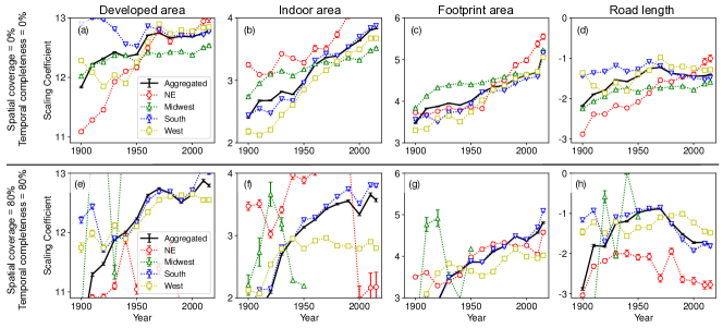
We also notice in Fig. 5 that the scaling coefficients vary strongly over time, most notably for developed, indoor, and building footprint areas. Given the stable scaling exponent this finding implies the developed and housing area per capita has increased over time, which is consistent to trends observed in the literature Moura \BOthers. (\APACyear2015). We independently confirm this finding using US Census data on newly built homes since 1978 (Supplementary Figure S5), in which we find the average area of houses sold has consistently increased until 2010–2015.
We also notice in Fig. 5 that developed area continues to increase over time, with one of the largest jumps occurring between 1950–1960. The coefficient change of implies developed area per capita increased by around 65%. This finding is consistent with literature on post-WWII housing boom Moffatt (\APACyear2021), and white flight Frey (\APACyear1979), which have contributed to a greater build-up of housing in suburbs and less-developed areas, after controlling for city population. Finally, we notice that the road length has recently decreased for cities even as their developed area stagnates. This might imply that cities have more recently become more sparse, but more work needs to be done to confirm these findings. Scaling coefficients are therefore not universal and vary strongly over time. The increase of coefficients also implies a greater amount of land used for contemporary development than in a comparable city in the year 1900.
Spatial Variations in Cross-Sectional Scaling
In order to test spatial and temporal variation of scaling laws, we ran our analysis for the different regions within the CONUS. We show an example of this in Fig. 4, in which we compare scaling laws based on all cities (“aggregated”) to scaling laws based on cities within the Northeast, Midwest, South, and West. Scaling law exponents consistently differ between regions; exponents in 2015 are statistically significantly different across regions (z-score p-values). Surprisingly, we find that the Northeast has consistently higher scaling exponents while the South and West have lower exponents. These lower exponents imply the South or West may have a greater economy of scale because their area or road length per capita is smaller for larger cities, thus they better (or more efficiently) utilize the infrastructure they have.
Furthermore, we also notice in Fig. 5 that the South and West have the highest coefficients, which implies that cities take up more space in these regions compared to similarly-sized cities in other regions. The most compact cities are therefore in the North-East, which have less developed area (and subsequently fewer roads), as well as smaller building footprints, than other regions. While North-Eastern cities were compact, they also initially had higher indoor area (e.g., larger houses). This did not change drastically over time, in contrast to other regions, leading North-Eastern cities to ultimately have lower indoor area than similar cities in other regions by 2015.
Discussion and Conclusions
In this study, we have tested the robustness of scaling laws over space and time. Our empirical definition of cities accounts for cities expanding and evolving, thus capturing when cities expand beyond and across administrative boundaries. In agreement with theoretical models Bettencourt (\APACyear2013), we find scaling law exponents do not change significantly over time. Scaling exponents, however, vary across space, possibly due to topographic constraints such as rivers or mountains, which can affect urban density Angel \BOthers. (\APACyear2017), but also other constraining factors. This builds on some recent research that finds temporally stable but spatially varying emergent urban patterns Barthelemy (\APACyear2019), such as in population dynamics Reia \BOthers. (\APACyear2022).
The long time window we analyze allows us to explore an under-appreciated component of scaling: the scaling coefficient (in contrast to the scaling exponent) shows an increase over time for most features, as seen in Fig. 4. Therefore, developed area, indoor floor area, building footprint area, and road length per capita are increasing on average. This reduces the amount of otherwise undeveloped land, which complicates resource use and harms the local environment, including water quality and wildlife habitat Glaeser \BBA Kahn (\APACyear2004); Lawler \BOthers. (\APACyear2014); Cumming \BOthers. (\APACyear2014). While previous work has found the developed land base has recently become denser Bigelow \BOthers. (\APACyear2022), our work implies that a city 100 years ago was still much more densely developed than the same city would be today. This reduced density is consistent with previous work on the loss of dense urban environments Angel \BOthers. (\APACyear2017). One reasonable hypothesis is that the reduced urban density is a function of increased car use throughout the century Schäfer (\APACyear2017), but we can only draw associations not cause and effect from these data, and previous work found car ownership can also be correlated with increasing urban density Angel \BOthers. (\APACyear2017). Therefore, more research is needed to better understand this trend.
These results have important consequences for the urban sciences. First, urban systems need to be studied based on historical data to fully understand their development trajectories. While previous work has made impressive advances in understanding historical urban development Ortman \BOthers. (\APACyear2020); J. Lobo \BOthers. (\APACyear2022, \APACyear2020); Smith \BOthers. (\APACyear2021), there has been a lack of analysis on scaling laws for the same cities over time. Our analysis exploits recently created historical urban data, which allows scaling comparisons to be performed for the same cities over a century. More analysis of this type, especially for superscaling variables like income Keuschnigg (\APACyear2019); Bettencourt \BOthers. (\APACyear2007) need to be explored. Finally, regional variations need to be explored. While universal laws are idealized explanations of urban science, regional variations can give insights into region-specific conditions. This can improve the interplay between urban science and policy-makers who focus on region- and city-specific problems.
There are certain limitations in the data we analyze. For example, built years are missing for many records, and the historical data exhibits survivorship bias Boeing (\APACyear2020\APACexlab\BCnt1). Furthermore, we assume that roads were constructed at approximately the same time as nearby buildings and that population is proportional to the number of buildings within a given city. We evaluated the reliability of such assumptions to the best of our ability, but more research is needed to test and improve upon them. For example, it is important to uncover new ways to approximate city populations as well as city features over time. In addition, our analysis of city-wide features belies variations within cities that need to be further analyzed and modeled Xue \BOthers. (\APACyear2022). Finally, there are several other features of cities, including economic indicators or road topology Scheer (\APACyear2001); Geiger \BOthers. (\APACyear2020); Xue \BOthers. (\APACyear2022), that could be explored in future work.
Materials and Methods
Historical urban boundary modeling. We modeled historical urban boundaries based on the historical, generalized built-up areas (GBUA; Uhl \BBA Burghardt (\APACyear2022)), which are based on the Historical Settlement Data Compilation for the US (HISDAC-US; Leyk \BBA Uhl (\APACyear2018\APACexlab\BCnt1)). Specifically, the GBUA dataset has been created by generating focal built-up density layers using gridded data on built-up areas Uhl \BBA Leyk (\APACyear2020\APACexlab\BCnt1) available in a grid of cells of 250 m x 250 m, in 5-year intervals from 1900 to 2010, using a circular focal window of 1km radius. From these built-up density layers, only areas of % built-up density were retained, to exclude low-density, scattered rural settlements. The remaining grid cells (delineating higher density settlements) were then segmented to obtain vector objects for each group of contiguous higher density grid cells (called “patches”). For each patch, we calculated the total number of buildings contained in it (using historical building counts from HISDAC-US i.e., the Built-Up Property Location (BUPL) layers, Uhl \BBA Leyk (\APACyear2020\APACexlab\BCnt2)) using a GIS-based zonal statistics tool, and ranked the patches by the number of buildings. Finally, we retained the upper 10% of these ranked patches, representing the high-density patches only. This process was done separately within each 2010 CBSA polygon C. Bureau (\APACyear2015). Lastly, the patches in all CBSAs were dissolved based on adjacency only, creating natural, contiguous built-up patches i.e., potentially extending across CBSA boundaries. This process was done for each point in time.
Historical population modeling. We acquired historical population counts at the US county level (boundaries of 2010, National Historical Geographic Information System Manson (\APACyear2020)) and aggregated the county populations by CBSA to obtain population time series for each 2010 CBSA boundary, for each decade from 1900 to 2010 (from the decennial censuses) and for 2015 (from the American Community Survey) U.C. Bureau (\APACyear2020\APACexlab\BCnt2, \APACyear2020\APACexlab\BCnt1, \APACyear2020\APACexlab\BCnt3). We spatially refined these CBSA-level population counts, for each point in time. To do so, we carried out a dasymetric refinement Maantay \BOthers. (\APACyear2007); Wei \BOthers. (\APACyear2017); Huang \BOthers. (\APACyear2021) by constraining the population estimates reported for the CBSAs to the generalized built-up areas of the respective year, within each CBSA, and assigning population counts to each patch proportionally to the number of built-up property records Uhl \BBA Leyk (\APACyear2020\APACexlab\BCnt3). The BUPR variable counts the number of built-up cadastral properties within each grid cell, and thus, approximates the spatial distribution of built-up structures, or cadastral parcels, or address points, which have been used for dasymetric modeling in previous work (e.g., Maantay \BOthers. (\APACyear2007); Wei \BOthers. (\APACyear2017); Huang \BOthers. (\APACyear2021); Zandbergen (\APACyear2011); Tapp (\APACyear2010); Yin \BOthers. (\APACyear2015)). Moreover, previous work has revealed strongly linear correlations between the number of houses within a spatial unit and its population over long time periods (Leyk \BOthers. (\APACyear2020); see also Supplementary Figure S1). Our historical, dasymetrically refined population estimates per city represent unique, long-term depictions of urban populations at fine spatial grain, and are in strong agreement with more sophisticated population estimations, shown in Supplementary Figure S2. Finally, we calculated the refined population estimates for the cities.
Historical built environment characteristics. We used three variables to historically characterize the built environment within each urban area representation: (a) developed area (measured by the number of built-up grid cells from the HISDAC-US Built-Up Area (BUA) layers, per CBSA polygon, for each year; (b) indoor area (measured by the built-up intensity layer from HISDAC-US; Built-Up Intensity (indoor area) Leyk \BBA Uhl (\APACyear2018\APACexlab\BCnt2), which reports the total indoor area of all builings within a grid cell, per year); and (c) building footprint area per grid cell and year Uhl \BBA Leyk (\APACyear2022). To obtain the latter, we spatially integrated cadastral data (containing construction year information) available at discrete, point-based locations from the Zillow Transaction and Assessment Dataset (ZTRAX; Zillow Inc. (\APACyear2016)), with vector data representing each building footprint in the US from Microsoft Microsoft (\APACyear2020). This integration assigns the thematic information from each ZTRAX record to the closest building footprint and thus, allowed us to merge the attribute richness of ZTRAX with the fine spatial detail of the USBuildingFootprints dataset. Using these integrated spatial data, we were able to stratify the building footprint data by their construction year and calculated the aggregated building footprint area within each grid cell as defined by the HISDAC-US 250 m x 250 m grid. For each of the gridded surfaces measuring developed area, indoor area, and building footprint area, for each year, we calculated zonal sums in a GIS, within each patch of the respective year. These zonal sums were then further aggregated to a city based on the recorded spatial relationships.
Historical road network modeling. In order to model historical road network densities, we followed a method proposed in Burghardt et al. Burghardt \BOthers. (\APACyear2022). Specifically, we clipped contemporary road network vector data from the National Transportation Dataset U.S. Geological Survey (\APACyear2018) to the historical urban delineations from the generalized urban area dataset for each year, and calculated the sum of the road network segment lengths per patch and year. We then aggregated these road network length estimates to the city based on the recorded spatial relationships (cf. Burghardt \BBA Uhl (\APACyear2022)). We show scatter plots of relationships between urban characteristics in Supplementary Figure S6 for 1900 and 2015.
Multi-temporal, cross-sectional scaling analysis. To find scaling laws between population estimates and the metrics describing the historical urban built environment and road network, we took the log of the feature versus the estimated population within the city and computed the least-squares fit of these trends, for each point of time. The slope of this line corresponds to the exponent of the scaling law. Namely, let be the city feature (e.g., developed area), and be the population. We fitted as the linear fit of . The y-intercept is , while the exponent, describes the slope. For regional stratification of our scaling results, we used geospatial data on Census Regions in the US C. Bureau (\APACyear2018).
Uncertainty quantification, cross-comparison and validation. Data Coverage and quality. Approximately 10% of US counties have low geographic coverage, or low completeness of construction date information (i.e., temporal coverage) in HISDAC-US and the underlying ZTRAX data. These completeness issues have been extensively studied in Boeing (\APACyear2020\APACexlab\BCnt1); Burghardt \BOthers. (\APACyear2022); Leyk \BBA Uhl (\APACyear2018\APACexlab\BCnt1)). We excluded CBSAs affected by these incompleteness issues from our analyses using a geospatial completeness threshold of 40% and temporal coverage of 60%. Out of 857 CBSAs, 647 were complete enough for analysis. Settlement density-based city patches, however, can span CBSAs with both high and low temporal coverage or geospatial completeness, therefore we created a weighted average estimate of the temporal coverage or geospatial completeness for each city. The weight was given by the number of patches within each CBSA that make up a given city. We then thresholded these weighted values to have temporal coverage above 60% and geospatial completeness above 40%.
We conducted a sensitivity analysis showing that our results are largely robust to the choice of this exclusion threshold (Supplementary Figures S3 & S4). Given the robustness of our results, we do not believe data completeness strongly affects our conclusions. Moreover, the BUPR, BUPL, BUA, and indoor area layers have been validated extensively in prior work Uhl \BOthers. (\APACyear2021) and show high levels of coherence to other historical measurements of population and building characteristics. Effects of survivorship bias (i.e., the limitation of the HISDAC-US to measure urban shrinkage and historical changes in the built environment) are assumed to be of minor nature (e.g., Burghardt \BOthers. (\APACyear2022); Boeing (\APACyear2020\APACexlab\BCnt2); Barrington-Leigh \BBA Millard-Ball (\APACyear2015); Meijer \BOthers. (\APACyear2018)). Historical road network models have been cross-compared to other models and datasets in Burghardt \BOthers. (\APACyear2022) reporting that there is sufficient consistency between these products.
Code for all our analysis can be found at:https://github.com/KeithBurghardt/urbanscaling.
Data Availability
The data is available in the following references: US regions C. Bureau (\APACyear2018), population U.C. Bureau (\APACyear2020\APACexlab\BCnt2, \APACyear2020\APACexlab\BCnt1, \APACyear2020\APACexlab\BCnt3), BUPR Uhl \BBA Leyk (\APACyear2020\APACexlab\BCnt3), BUPL Uhl \BBA Leyk (\APACyear2020\APACexlab\BCnt2), BUA Uhl \BBA Leyk (\APACyear2020\APACexlab\BCnt1), footprint area Uhl \BBA Leyk (\APACyear2022), and indoor area Leyk \BBA Uhl (\APACyear2018\APACexlab\BCnt2), road networks Burghardt \BBA Uhl (\APACyear2022), and patch boundaries Uhl \BBA Burghardt (\APACyear2022). SI data for house sizes since 1978 are from Census Bureau (\APACyear2021). In these data, references to patches are density-based settlements within a CBSA. Merging any neighboring cross-CBSA patches (using Uhl \BBA Burghardt (\APACyear2022)) creates the city features we analyze in this paper.
Competing Interests
The Authors declare no competing financial or non-financial interests.
Author Contributions
K.B., J.U., K.L., and S.L. designed research; K.B. and J.U. performed analysis; K.B., J.U., K.L., and S.L. wrote the paper.
Acknowledgements
Partial funding for this work was provided through the National Science Foundation (awards 1924670 and 2121976) and the Eunice Kennedy Shriver National Institute of Child Health and Human Development of the National Institutes of Health under award number P2CHD066613. The content is solely the responsibility of the authors and does not necessarily represent the official views of the National Institutes of Health. Moreover, Safe Software, Inc., is acknowledged for providing a Feature Manipulation Engine (FME) Desktop license used for data processing.


References
- \bibcommenthead
- Angel \BOthers. (\APACyear2017) \APACinsertmetastarAngel2017{APACrefauthors}Angel, S., Parent, J., Civco, D.L.\BCBL Blei, A. \APACrefYearMonthDay2017. \APACrefbtitleThe Persistent Decline in Urban Densities: Global and Historical Evidence of ’Sprawl’. The persistent decline in urban densities: Global and historical evidence of ’sprawl’. \APACaddressPublisherThe Lincoln Institute of Land Policy. \PrintBackRefs\CurrentBib
- Arcaute \BOthers. (\APACyear2015) \APACinsertmetastarArcaute2015{APACrefauthors}Arcaute, E., Hatna, E., Ferguson, P., Youn, H., Johansson, A.\BCBL Batty, M. \APACrefYearMonthDay2015. \BBOQ\APACrefatitleConstructing cities, deconstructing scaling laws Constructing cities, deconstructing scaling laws.\BBCQ \APACjournalVolNumPagesJournal of The Royal Society Interface1210220140745. {APACrefURL} https://royalsocietypublishing.org/doi/abs/10.1098/rsif.2014.0745 https://royalsocietypublishing.org/doi/pdf/10.1098/rsif.2014.0745 {APACrefDOI} 10.1098/rsif.2014.0745 \PrintBackRefs\CurrentBib
- Barrington-Leigh \BBA Millard-Ball (\APACyear2015) \APACinsertmetastarbarrington2015century{APACrefauthors}Barrington-Leigh, C.\BCBT \BBA Millard-Ball, A. \APACrefYearMonthDay2015. \BBOQ\APACrefatitleA century of sprawl in the United States A century of sprawl in the united states.\BBCQ \APACjournalVolNumPagesProceedings of the National Academy of Sciences112278244–8249. \PrintBackRefs\CurrentBib
- Barthelemy (\APACyear2019) \APACinsertmetastarBarthelemy2019{APACrefauthors}Barthelemy, M. \APACrefYearMonthDay2019. \BBOQ\APACrefatitleThe statistical physics of cities The statistical physics of cities.\BBCQ \APACjournalVolNumPagesNature Reviews Physics16406–415. {APACrefURL} https://doi.org/10.1038/s42254-019-0054-2 {APACrefDOI} 10.1038/s42254-019-0054-2 \PrintBackRefs\CurrentBib
- Batty (\APACyear2006) \APACinsertmetastarBatty2006{APACrefauthors}Batty, M. \APACrefYearMonthDay2006. \BBOQ\APACrefatitleRank clocks Rank clocks.\BBCQ \APACjournalVolNumPagesNature4447119592–596. {APACrefURL} https://doi.org/10.1038/nature05302 {APACrefDOI} 10.1038/nature05302 \PrintBackRefs\CurrentBib
- Baynes \BOthers. (\APACyear2022) \APACinsertmetastarBaynes2022{APACrefauthors}Baynes, J., Neale, A.\BCBL Hultgren, T. \APACrefYearMonthDay2022. \BBOQ\APACrefatitleImproving intelligent dasymetric mapping population density estimates at 30 m resolution for the conterminous United States by excluding uninhabited areas Improving intelligent dasymetric mapping population density estimates at 30 m resolution for the conterminous united states by excluding uninhabited areas.\BBCQ \APACjournalVolNumPagesEarth System Science Data1462833–2849. {APACrefURL} https://essd.copernicus.org/articles/14/2833/2022/ {APACrefDOI} 10.5194/essd-14-2833-2022 \PrintBackRefs\CurrentBib
- Bettencourt (\APACyear2013) \APACinsertmetastarBettencourt2013{APACrefauthors}Bettencourt, L.M.A. \APACrefYearMonthDay2013. \BBOQ\APACrefatitleThe Origins of Scaling in Cities The origins of scaling in cities.\BBCQ \APACjournalVolNumPagesScience34061391438–1441. {APACrefURL} https://science.sciencemag.org/content/340/6139/1438 https://science.sciencemag.org/content/340/6139/1438.full.pdf {APACrefDOI} 10.1126/science.1235823 \PrintBackRefs\CurrentBib
- Bettencourt \BOthers. (\APACyear2007) \APACinsertmetastarBettencourt2007{APACrefauthors}Bettencourt, L.M.A., Lobo, J., Helbing, D., Kühnert, C.\BCBL West, G.B. \APACrefYearMonthDay2007. \BBOQ\APACrefatitleGrowth, innovation, scaling, and the pace of life in cities Growth, innovation, scaling, and the pace of life in cities.\BBCQ \APACjournalVolNumPagesProceedings of the National Academy of Sciences104177301–7306. {APACrefURL} https://www.pnas.org/content/104/17/7301 https://www.pnas.org/content/104/17/7301.full.pdf {APACrefDOI} 10.1073/pnas.0610172104 \PrintBackRefs\CurrentBib
- Bettencourt \BOthers. (\APACyear2020) \APACinsertmetastarBettencourt2020_longvscross{APACrefauthors}Bettencourt, L.M.A., Yang, V.C., Lobo, J., Kempes, C.P., Rybski, D.\BCBL Hamilton, M.J. \APACrefYearMonthDay2020. \BBOQ\APACrefatitleThe interpretation of urban scaling analysis in time The interpretation of urban scaling analysis in time.\BBCQ \APACjournalVolNumPagesJournal of The Royal Society Interface1716320190846. {APACrefURL} https://royalsocietypublishing.org/doi/abs/10.1098/rsif.2019.0846 https://royalsocietypublishing.org/doi/pdf/10.1098/rsif.2019.0846 {APACrefDOI} 10.1098/rsif.2019.0846 \PrintBackRefs\CurrentBib
- Bigelow \BOthers. (\APACyear2022) \APACinsertmetastarBigelow2022{APACrefauthors}Bigelow, D.P., Lewis, D.J.\BCBL Mihiar, C. \APACrefYearMonthDay2022jan. \BBOQ\APACrefatitleA major shift in U.S. land development avoids significant losses in forest and agricultural land A major shift in u.s. land development avoids significant losses in forest and agricultural land.\BBCQ \APACjournalVolNumPagesEnvironmental Research Letters172024007. {APACrefURL} https://doi.org/10.1088/1748-9326/ac4537 {APACrefDOI} 10.1088/1748-9326/ac4537 \PrintBackRefs\CurrentBib
- Boeing (\APACyear2020\APACexlab\BCnt1) \APACinsertmetastarBoeing2020multi{APACrefauthors}Boeing, G. \APACrefYearMonthDay2020\BCnt1. \BBOQ\APACrefatitleA multi-scale analysis of 27,000 urban street networks: Every US city, town, urbanized area, and Zillow neighborhood A multi-scale analysis of 27,000 urban street networks: Every us city, town, urbanized area, and zillow neighborhood.\BBCQ \APACjournalVolNumPagesEnvironment and Planning B: Urban Analytics and City Science474590-608. {APACrefDOI} 10.1177/2399808318784595 \PrintBackRefs\CurrentBib
- Boeing (\APACyear2020\APACexlab\BCnt2) \APACinsertmetastarboeing2020off{APACrefauthors}Boeing, G. \APACrefYearMonthDay2020\BCnt2. \BBOQ\APACrefatitleOff the Grid…and Back Again? The Recent Evolution of American Street Network Planning and Design Off the grid…and back again? the recent evolution of american street network planning and design.\BBCQ \APACjournalVolNumPagesJournal of the American Planning Association8711–15. \PrintBackRefs\CurrentBib
- C. Bureau (\APACyear2015) \APACinsertmetastarCBSA{APACrefauthors}Bureau, C. \APACrefYearMonthDay2015. \APACrefbtitletl_2015_us_cbsa. tl_2015_us_cbsa. \APAChowpublishedhttps://www2.census.gov/geo/tiger/TIGER2015/CBSA/. \PrintBackRefs\CurrentBib
- C. Bureau (\APACyear2018) \APACinsertmetastarCensusRegions{APACrefauthors}Bureau, C. \APACrefYearMonthDay2018. \APACrefbtitlecb_2018_us_region_500k. cb_2018_us_region_500k. \APAChowpublishedhttps://www2.census.gov/geo/tiger/GENZ2018/shp/cb_2018_us_region_500k.zip. \PrintBackRefs\CurrentBib
- U.C. Bureau (\APACyear2020\APACexlab\BCnt1) \APACinsertmetastarcensus_county_pop_mid{APACrefauthors}Bureau, U.C. \APACrefYearMonthDay2020\BCnt1. \APACrefbtitlecenpop2000. cenpop2000. \APAChowpublishedhttps://www2.census.gov/geo/docs/reference/cenpop2000/county/. \PrintBackRefs\CurrentBib
- U.C. Bureau (\APACyear2020\APACexlab\BCnt2) \APACinsertmetastarcensus_county_pop_old{APACrefauthors}Bureau, U.C. \APACrefYearMonthDay2020\BCnt2. \APACrefbtitleCensus U.S. Decennial County Population Data, 1900-1990. Census u.s. decennial county population data, 1900-1990. \APAChowpublishedhttps://www.nber.org/research/data/census-us-decennial-county-population-data-1900-1990. \PrintBackRefs\CurrentBib
- U.C. Bureau (\APACyear2020\APACexlab\BCnt3) \APACinsertmetastarcensus_county_pop_new{APACrefauthors}Bureau, U.C. \APACrefYearMonthDay2020\BCnt3. \APACrefbtitleCounty Population Totals: 2010-2019. County population totals: 2010-2019. \APAChowpublishedhttps://www.census.gov/data/tables/time-series/demo/popest/2010s-counties-total.html. \PrintBackRefs\CurrentBib
- Burghardt \BBA Uhl (\APACyear2022) \APACinsertmetastarBurghardt2022_roadstats{APACrefauthors}Burghardt, K.\BCBT \BBA Uhl, J.H. \APACrefYearMonthDay2022. \APACrefbtitleHistorical road network statistics for core-based statistical areas in the U.S. (1900 - 2010). Historical road network statistics for core-based statistical areas in the u.s. (1900 - 2010). \APACrefnoteOnline; accessed 01 January 2023 {APACrefDOI} 10.6084/m9.figshare.19584088.v1 \PrintBackRefs\CurrentBib
- Burghardt \BOthers. (\APACyear2022) \APACinsertmetastarBurghardt2021_city{APACrefauthors}Burghardt, K., Uhl, J.H., Lerman, K.\BCBL Leyk, S. \APACrefYearMonthDay2022. \BBOQ\APACrefatitleRoad network evolution in the urban and rural United States since 1900 Road network evolution in the urban and rural united states since 1900.\BBCQ \APACjournalVolNumPagesComputers, Environment and Urban Systems95101803. {APACrefDOI} https://doi.org/10.1016/j.compenvurbsys.2022.101803 \PrintBackRefs\CurrentBib
- Census Bureau (\APACyear2021) \APACinsertmetastarHouseArea{APACrefauthors}Census Bureau \APACrefYearMonthDay2021. \APACrefbtitleCharacteristics of New Housing. Characteristics of new housing. \APAChowpublishedhttps://www.census.gov/construction/chars/. \PrintBackRefs\CurrentBib
- Cottineau \BOthers. (\APACyear2017) \APACinsertmetastarCottineau2017{APACrefauthors}Cottineau, C., Hatna, E., Arcaute, E.\BCBL Batty, M. \APACrefYearMonthDay2017. \BBOQ\APACrefatitleDiverse cities or the systematic paradox of Urban Scaling Laws Diverse cities or the systematic paradox of urban scaling laws.\BBCQ \APACjournalVolNumPagesComputers, Environment and Urban Systems6380-94. \APACrefnoteSpatial analysis with census data: emerging issues and innovative approaches \PrintBackRefs\CurrentBib
- Cumming \BOthers. (\APACyear2014) \APACinsertmetastarcumming2014implications{APACrefauthors}Cumming, G.S., Buerkert, A., Hoffmann, E.M., Schlecht, E., von Cramon-Taubadel, S.\BCBL Tscharntke, T. \APACrefYearMonthDay2014. \BBOQ\APACrefatitleImplications of agricultural transitions and urbanization for ecosystem services Implications of agricultural transitions and urbanization for ecosystem services.\BBCQ \APACjournalVolNumPagesNature515752550–57. \PrintBackRefs\CurrentBib
- Depersin \BBA Barthelemy (\APACyear2018) \APACinsertmetastarDepersin2018{APACrefauthors}Depersin, J.\BCBT \BBA Barthelemy, M. \APACrefYearMonthDay2018. \BBOQ\APACrefatitleFrom global scaling to the dynamics of individual cities From global scaling to the dynamics of individual cities.\BBCQ \APACjournalVolNumPagesProceedings of the National Academy of Sciences115102317–2322. {APACrefURL} https://www.pnas.org/content/115/10/2317 https://www.pnas.org/content/115/10/2317.full.pdf {APACrefDOI} 10.1073/pnas.1718690115 \PrintBackRefs\CurrentBib
- Eeckhout (\APACyear2004) \APACinsertmetastarEeckhout2004{APACrefauthors}Eeckhout, J. \APACrefYearMonthDay2004December. \BBOQ\APACrefatitleGibrat’s Law for (All) Cities Gibrat’s law for (all) cities.\BBCQ \APACjournalVolNumPagesAmerican Economic Review9451429-1451. {APACrefURL} https://www.aeaweb.org/articles?id=10.1257/0002828043052303 {APACrefDOI} 10.1257/0002828043052303 \PrintBackRefs\CurrentBib
- El Gouj \BOthers. (\APACyear2022) \APACinsertmetastarGouj2022{APACrefauthors}El Gouj, H., Rincón-Acosta, C.\BCBL Lagesse, C. \APACrefYearMonthDay2022. \BBOQ\APACrefatitleUrban morphogenesis analysis based on geohistorical road data Urban morphogenesis analysis based on geohistorical road data.\BBCQ \APACjournalVolNumPagesApplied Network Science716. {APACrefURL} https://doi.org/10.1007/s41109-021-00440-0 {APACrefDOI} 10.1007/s41109-021-00440-0 \PrintBackRefs\CurrentBib
- Frey (\APACyear1979) \APACinsertmetastarFrey1979{APACrefauthors}Frey, W.H. \APACrefYearMonthDay1979. \BBOQ\APACrefatitleCentral City White Flight: Racial and Nonracial Causes Central city white flight: Racial and nonracial causes.\BBCQ \APACjournalVolNumPagesAmerican Sociological Review443425–448. {APACrefURL} [2022-09-14]http://www.jstor.org/stable/2094885 \PrintBackRefs\CurrentBib
- Gabaix \BBA Ioannides (\APACyear2004) \APACinsertmetastarGabaix2004{APACrefauthors}Gabaix, X.\BCBT \BBA Ioannides, Y.M. \APACrefYearMonthDay2004. \BBOQ\APACrefatitleChapter 53 - The Evolution of City Size Distributions Chapter 53 - the evolution of city size distributions.\BBCQ J.V. Henderson \BBA J\BHBIF. Thisse (\BEDS), \APACrefbtitleCities and Geography Cities and geography (\BVOL 4, \BPG 2341-2378). \APACaddressPublisherElsevier. {APACrefURL} https://www.sciencedirect.com/science/article/pii/S1574008004800105 {APACrefDOI} https://doi.org/10.1016/S1574-0080(04)80010-5 \PrintBackRefs\CurrentBib
- Geiger \BOthers. (\APACyear2020) \APACinsertmetastarGeiger2020{APACrefauthors}Geiger, B.C., Jang, G.U., Joo, J.C.\BCBL Park, J. \APACrefYearMonthDay2020. \BBOQ\APACrefatitleCapturing the Signature of Topological Evolution from the Snapshots of Road Networks Capturing the signature of topological evolution from the snapshots of road networks.\BBCQ \APACjournalVolNumPagesComplexity20208054316. {APACrefURL} https://doi.org/10.1155/2020/8054316 {APACrefDOI} 10.1155/2020/8054316 \PrintBackRefs\CurrentBib
- Glaeser \BBA Kahn (\APACyear2004) \APACinsertmetastarglaeser2004sprawl{APACrefauthors}Glaeser, E.L.\BCBT \BBA Kahn, M.E. \APACrefYearMonthDay2004. \BBOQ\APACrefatitleSprawl and urban growth Sprawl and urban growth.\BBCQ \APACrefbtitleHandbook of regional and urban economics Handbook of regional and urban economics (\BVOL 4, \BPGS 2481–2527). \APACaddressPublisherElsevier. \PrintBackRefs\CurrentBib
- González \BOthers. (\APACyear2008) \APACinsertmetastarGonzalez2009{APACrefauthors}González, M.C., Hidalgo, C.A.\BCBL Barabási, A\BHBIL. \APACrefYearMonthDay2008. \BBOQ\APACrefatitleUnderstanding individual human mobility patterns Understanding individual human mobility patterns.\BBCQ \APACjournalVolNumPagesNature4537196779–782. {APACrefURL} https://doi.org/10.1038/nature06958 {APACrefDOI} 10.1038/nature06958 \PrintBackRefs\CurrentBib
- Huang \BOthers. (\APACyear2021) \APACinsertmetastarHuang2021{APACrefauthors}Huang, X., Wang, C., Li, Z.\BCBL Ning, H. \APACrefYearMonthDay2021. \BBOQ\APACrefatitleA 100 m population grid in the CONUS by disaggregating census data with open-source Microsoft building footprints A 100 m population grid in the conus by disaggregating census data with open-source microsoft building footprints.\BBCQ \APACjournalVolNumPagesBig Earth Data51112-133. \PrintBackRefs\CurrentBib
- Jia \BBA Jiang (\APACyear2010) \APACinsertmetastarJiang2010{APACrefauthors}Jia, T.\BCBT \BBA Jiang, B. \APACrefYearMonthDay2010. \BBOQ\APACrefatitleMeasuring urban sprawl based on massive street nodes and the novel concept of natural cities Measuring urban sprawl based on massive street nodes and the novel concept of natural cities.\BBCQ \APACjournalVolNumPagesarXiv preprint arXiv:1010.0541. \PrintBackRefs\CurrentBib
- Jiang \BBA Jia (\APACyear2011) \APACinsertmetastarJiang2011{APACrefauthors}Jiang, B.\BCBT \BBA Jia, T. \APACrefYearMonthDay2011. \BBOQ\APACrefatitleZipf’s law for all the natural cities in the United States: a geospatial perspective Zipf’s law for all the natural cities in the united states: a geospatial perspective.\BBCQ \APACjournalVolNumPagesInternational Journal of Geographical Information Science2581269-1281. {APACrefDOI} 10.1080/13658816.2010.510801 \PrintBackRefs\CurrentBib
- Jiang \BBA Miao (\APACyear2015) \APACinsertmetastarJiang2015_evol{APACrefauthors}Jiang, B.\BCBT \BBA Miao, Y. \APACrefYearMonthDay2015. \BBOQ\APACrefatitleThe Evolution of Natural Cities from the Perspective of Location-Based Social Media The evolution of natural cities from the perspective of location-based social media.\BBCQ \APACjournalVolNumPagesThe Professional Geographer672295-306. {APACrefDOI} 10.1080/00330124.2014.968886 \PrintBackRefs\CurrentBib
- Jiang \BOthers. (\APACyear2015) \APACinsertmetastarJiang2015_naturalworld{APACrefauthors}Jiang, B., Yin, J.\BCBL Liu, Q. \APACrefYearMonthDay2015. \BBOQ\APACrefatitleZipf’s law for all the natural cities around the world Zipf’s law for all the natural cities around the world.\BBCQ \APACjournalVolNumPagesInternational Journal of Geographical Information Science293498-522. {APACrefURL} https://doi.org/10.1080/13658816.2014.988715 https://doi.org/10.1080/13658816.2014.988715 {APACrefDOI} 10.1080/13658816.2014.988715 \PrintBackRefs\CurrentBib
- Jusup \BOthers. (\APACyear2022) \APACinsertmetastarJusup2022{APACrefauthors}Jusup, M., Holme, P., Kanazawa, K., Takayasu, M., Romić, I., Wang, Z.\BDBLPerc, M. \APACrefYearMonthDay2022. \BBOQ\APACrefatitleSocial physics Social physics.\BBCQ \APACjournalVolNumPagesPhysics Reports9481-148. {APACrefURL} https://www.sciencedirect.com/science/article/pii/S037015732100404X \APACrefnoteSocial physics {APACrefDOI} https://doi.org/10.1016/j.physrep.2021.10.005 \PrintBackRefs\CurrentBib
- Keuschnigg (\APACyear2019) \APACinsertmetastarKeuschnigg2019{APACrefauthors}Keuschnigg, M. \APACrefYearMonthDay2019. \BBOQ\APACrefatitleScaling trajectories of cities Scaling trajectories of cities.\BBCQ \APACjournalVolNumPagesProceedings of the National Academy of Sciences1162813759–13761. {APACrefURL} https://www.pnas.org/content/116/28/13759 https://www.pnas.org/content/116/28/13759.full.pdf {APACrefDOI} 10.1073/pnas.1906258116 \PrintBackRefs\CurrentBib
- Lawler \BOthers. (\APACyear2014) \APACinsertmetastarlawler2014projected{APACrefauthors}Lawler, J.J., Lewis, D.J., Nelson, E., Plantinga, A.J., Polasky, S., Withey, J.C.\BDBLRadeloff, V.C. \APACrefYearMonthDay2014. \BBOQ\APACrefatitleProjected land-use change impacts on ecosystem services in the United States Projected land-use change impacts on ecosystem services in the united states.\BBCQ \APACjournalVolNumPagesProceedings of the National Academy of Sciences111207492–7497. \PrintBackRefs\CurrentBib
- Leyk \BBA Uhl (\APACyear2018\APACexlab\BCnt1) \APACinsertmetastarleyk2018hisdac{APACrefauthors}Leyk, S.\BCBT \BBA Uhl, J.H. \APACrefYearMonthDay2018\BCnt1. \BBOQ\APACrefatitleHISDAC-US, historical settlement data compilation for the conterminous United States over 200 years Hisdac-us, historical settlement data compilation for the conterminous united states over 200 years.\BBCQ \APACjournalVolNumPagesScientific data5180175. \PrintBackRefs\CurrentBib
- Leyk \BBA Uhl (\APACyear2018\APACexlab\BCnt2) \APACinsertmetastardata_bui2018{APACrefauthors}Leyk, S.\BCBT \BBA Uhl, J.H. \APACrefYearMonthDay2018\BCnt2. \APACrefbtitleHistorical built-up intensity layer series for the U.S. 1810 - 2015. Historical built-up intensity layer series for the U.S. 1810 - 2015. \APACaddressPublisherHarvard Dataverse. {APACrefDOI} 10.7910/DVN/1WB9E4 \PrintBackRefs\CurrentBib
- Leyk \BOthers. (\APACyear2020) \APACinsertmetastarLeyk2020{APACrefauthors}Leyk, S., Uhl, J.H., Connor, D.S., Braswell, A.E., Mietkiewicz, N., Balch, J.K.\BCBL Gutmann, M. \APACrefYearMonthDay2020. \BBOQ\APACrefatitleTwo centuries of settlement and urban development in the United States Two centuries of settlement and urban development in the united states.\BBCQ \APACjournalVolNumPagesScience Advances623. {APACrefURL} https://advances.sciencemag.org/content/6/23/eaba2937 https://advances.sciencemag.org/content/6/23/eaba2937.full.pdf {APACrefDOI} 10.1126/sciadv.aba2937 \PrintBackRefs\CurrentBib
- Li \BOthers. (\APACyear2022) \APACinsertmetastarLi2022{APACrefauthors}Li, X., Tian, H., Pan, S.\BCBL Lu, C. \APACrefYearMonthDay2022. \BBOQ\APACrefatitleFour-century history of land transformation by humans in the United States: 1630–2020 Four-century history of land transformation by humans in the united states: 1630–2020.\BBCQ \APACjournalVolNumPagesEarth System Science Data Discussions20221–36. {APACrefURL} https://essd.copernicus.org/preprints/essd-2022-135/ {APACrefDOI} 10.5194/essd-2022-135 \PrintBackRefs\CurrentBib
- J. Lobo \BOthers. (\APACyear2020) \APACinsertmetastarLobo2020_scaling{APACrefauthors}Lobo, J., Bettencourt, L.M., Smith, M.E.\BCBL Ortman, S. \APACrefYearMonthDay2020. \BBOQ\APACrefatitleSettlement scaling theory: Bridging the study of ancient and contemporary urban systems Settlement scaling theory: Bridging the study of ancient and contemporary urban systems.\BBCQ \APACjournalVolNumPagesUrban Studies574731-747. {APACrefDOI} 10.1177/0042098019873796 \PrintBackRefs\CurrentBib
- J. Lobo \BOthers. (\APACyear2022) \APACinsertmetastarLobo2022_hunter{APACrefauthors}Lobo, J., Whitelaw, T., Bettencourt, L.M.A., Wiessner, P., Smith, M.E.\BCBL Ortman, S. \APACrefYearMonthDay2022. \BBOQ\APACrefatitleScaling of Hunter-Gatherer Camp Size and Human Sociality Scaling of hunter-gatherer camp size and human sociality.\BBCQ \APACjournalVolNumPagesCurrent Anthropology63168-94. {APACrefDOI} 10.1086/719234 \PrintBackRefs\CurrentBib
- J.e.a. Lobo (\APACyear2020) \APACinsertmetastarLobo2020_urban{APACrefauthors}Lobo, J.e.a. \APACrefYear2020. \APACrefbtitleUrban Science: Integrated Theory from the First Cities to Sustainable Metropolises Urban science: Integrated theory from the first cities to sustainable metropolises. {APACrefURL} http://dx.doi.org/10.2139/ssrn.3526940 {APACrefDOI} 10.2139/ssrn.3526940 \PrintBackRefs\CurrentBib
- Louf \BBA Barthelemy (\APACyear2014) \APACinsertmetastarLouf2014{APACrefauthors}Louf, R.\BCBT \BBA Barthelemy, M. \APACrefYearMonthDay2014. \BBOQ\APACrefatitleHow congestion shapes cities: from mobility patterns to scaling How congestion shapes cities: from mobility patterns to scaling.\BBCQ \APACjournalVolNumPagesScientific Reports415561. {APACrefURL} https://doi.org/10.1038/srep05561 {APACrefDOI} 10.1038/srep05561 \PrintBackRefs\CurrentBib
- Maantay \BOthers. (\APACyear2007) \APACinsertmetastarMaantay2007{APACrefauthors}Maantay, J.A., Maroko, A.R.\BCBL Herrmann, C. \APACrefYearMonthDay2007. \BBOQ\APACrefatitleMapping Population Distribution in the Urban Environment: The Cadastral-based Expert Dasymetric System (CEDS) Mapping population distribution in the urban environment: The cadastral-based expert dasymetric system (ceds).\BBCQ \APACjournalVolNumPagesCartography and Geographic Information Science34277-102. {APACrefURL} https://doi.org/10.1559/152304007781002190 https://doi.org/10.1559/152304007781002190 {APACrefDOI} 10.1559/152304007781002190 \PrintBackRefs\CurrentBib
- Manson (\APACyear2020) \APACinsertmetastarNHGIS{APACrefauthors}Manson, S. \APACrefYearMonthDay2020. \APACrefbtitleIPUMS National Historical Geographic Information System: Version 15.0 Ipums national historical geographic information system: Version 15.0 [Other]. \APACaddressPublisherIPUMS. \PrintBackRefs\CurrentBib
- Meijer \BOthers. (\APACyear2018) \APACinsertmetastarMeijer2018{APACrefauthors}Meijer, J.R., Huijbregts, M.A.J., Schotten, K.C.G.J.\BCBL Schipper, A.M. \APACrefYearMonthDay2018. \BBOQ\APACrefatitleGlobal patterns of current and future road infrastructure Global patterns of current and future road infrastructure.\BBCQ \APACjournalVolNumPagesEnvironmental Research Letters136064006. \PrintBackRefs\CurrentBib
- Microsoft (\APACyear2020) \APACinsertmetastarMBF2020{APACrefauthors}Microsoft \APACrefYearMonthDay2020. \APACrefbtitleUSBuildingFootprints. Usbuildingfootprints. \APAChowpublishedhttps://github.com/Microsoft/USBuildingFootprints. \PrintBackRefs\CurrentBib
- Moffatt (\APACyear2021) \APACinsertmetastarMoffatt2021{APACrefauthors}Moffatt, M. \APACrefYearMonthDay2021September8. \BBOQ\APACrefatitleWhat Caused the Post-War Economic Housing Boom After WWII? What caused the post-war economic housing boom after wwii?\BBCQ \APACjournalVolNumPagesThoughtCo. \APAChowpublishedthoughtco.com/the-post-war-us-economy-1945-to-1960-1148153. \PrintBackRefs\CurrentBib
- Montgomery (\APACyear2008) \APACinsertmetastarMontgomery2008{APACrefauthors}Montgomery, M.R. \APACrefYearMonthDay2008. \BBOQ\APACrefatitleThe Urban Transformation of the Developing World The urban transformation of the developing world.\BBCQ \APACjournalVolNumPagesScience3195864761-764. {APACrefURL} https://www.science.org/doi/abs/10.1126/science.1153012 https://www.science.org/doi/pdf/10.1126/science.1153012 {APACrefDOI} 10.1126/science.1153012 \PrintBackRefs\CurrentBib
- Moura \BOthers. (\APACyear2015) \APACinsertmetastarMoura2015{APACrefauthors}Moura, M.C.P., Smith, S.J.\BCBL Belzer, D.B. \APACrefYearMonthDay201508. \BBOQ\APACrefatitle120 Years of U.S. Residential Housing Stock and Floor Space 120 years of u.s. residential housing stock and floor space.\BBCQ \APACjournalVolNumPagesPLOS ONE1081-18. {APACrefURL} https://doi.org/10.1371/journal.pone.0134135 {APACrefDOI} 10.1371/journal.pone.0134135 \PrintBackRefs\CurrentBib
- of Economic \BBA Social Affairs (\APACyear2019) \APACinsertmetastarUN2019{APACrefauthors}of Economic, D.\BCBT \BBA Social Affairs, P.D. \APACrefYearMonthDay2019. \APACrefbtitleWorld Urbanization Prospects, The 2018 Revision. World urbanization prospects, the 2018 revision. \APACaddressPublisherNew YorkUnited Nations. \PrintBackRefs\CurrentBib
- Ortman \BOthers. (\APACyear2020) \APACinsertmetastarOrtman2020{APACrefauthors}Ortman, S.G., Lobo, J.\BCBL Smith, M.E. \APACrefYearMonthDay202012. \BBOQ\APACrefatitleCities: Complexity, theory and history Cities: Complexity, theory and history.\BBCQ \APACjournalVolNumPagesPLOS ONE15121-24. {APACrefURL} https://doi.org/10.1371/journal.pone.0243621 {APACrefDOI} 10.1371/journal.pone.0243621 \PrintBackRefs\CurrentBib
- Parr (\APACyear2007) \APACinsertmetastarparr2007spatial{APACrefauthors}Parr, J.B. \APACrefYearMonthDay2007. \BBOQ\APACrefatitleSpatial definitions of the city: four perspectives Spatial definitions of the city: four perspectives.\BBCQ \APACjournalVolNumPagesUrban studies442381–392. \PrintBackRefs\CurrentBib
- Reia \BOthers. (\APACyear2022) \APACinsertmetastarReia2022{APACrefauthors}Reia, S.M., Rao, P.S.C.\BCBL Ukkusuri, S.V. \APACrefYearMonthDay2022. \BBOQ\APACrefatitleModeling the dynamics and spatial heterogeneity of city growth Modeling the dynamics and spatial heterogeneity of city growth.\BBCQ \APACjournalVolNumPagesnpj Urban Sustainability2131. {APACrefURL} https://doi.org/10.1038/s42949-022-00075-9 {APACrefDOI} 10.1038/s42949-022-00075-9 \PrintBackRefs\CurrentBib
- Rozenfeld \BOthers. (\APACyear2008) \APACinsertmetastarRozenfeld2008{APACrefauthors}Rozenfeld, H.D., Rybski, D., Andrade, J.S., Batty, M., Stanley, H.E.\BCBL Makse, H.A. \APACrefYearMonthDay2008. \BBOQ\APACrefatitleLaws of population growth Laws of population growth.\BBCQ \APACjournalVolNumPagesProceedings of the National Academy of Sciences1054818702–18707. {APACrefURL} https://www.pnas.org/content/105/48/18702 https://www.pnas.org/content/105/48/18702.full.pdf {APACrefDOI} 10.1073/pnas.0807435105 \PrintBackRefs\CurrentBib
- Rozenfeld \BOthers. (\APACyear2011) \APACinsertmetastarRozenfeld2011{APACrefauthors}Rozenfeld, H.D., Rybski, D., Gabaix, X.\BCBL Makse, H.A. \APACrefYearMonthDay2011. \BBOQ\APACrefatitleThe area and population of cities: New insights from a different perspective on cities The area and population of cities: New insights from a different perspective on cities.\BBCQ \APACjournalVolNumPagesAmerican Economic Review1012205–2225. \PrintBackRefs\CurrentBib
- Schäfer (\APACyear2017) \APACinsertmetastarSchafer2017{APACrefauthors}Schäfer, A.W. \APACrefYearMonthDay2017. \BBOQ\APACrefatitleLong-term trends in domestic US passenger travel: the past 110 years and the next 90 Long-term trends in domestic us passenger travel: the past 110 years and the next 90.\BBCQ \APACjournalVolNumPagesTransportation442293–310. {APACrefURL} https://doi.org/10.1007/s11116-015-9638-6 {APACrefDOI} 10.1007/s11116-015-9638-6 \PrintBackRefs\CurrentBib
- Scheer (\APACyear2001) \APACinsertmetastarscheer2001anatomy{APACrefauthors}Scheer, B.C. \APACrefYearMonthDay2001. \BBOQ\APACrefatitleThe anatomy of sprawl The anatomy of sprawl.\BBCQ \APACjournalVolNumPagesPlaces142. \PrintBackRefs\CurrentBib
- Small \BOthers. (\APACyear2005) \APACinsertmetastarSmall2005{APACrefauthors}Small, C., Pozzi, F.\BCBL Elvidge, C. \APACrefYearMonthDay2005. \BBOQ\APACrefatitleSpatial analysis of global urban extent from DMSP-OLS night lights Spatial analysis of global urban extent from dmsp-ols night lights.\BBCQ \APACjournalVolNumPagesRemote Sensing of Environment963277-291. {APACrefURL} https://www.sciencedirect.com/science/article/pii/S0034425705000696 {APACrefDOI} https://doi.org/10.1016/j.rse.2005.02.002 \PrintBackRefs\CurrentBib
- Smith \BOthers. (\APACyear2021) \APACinsertmetastarsmith2021{APACrefauthors}Smith, M.E., Ortman, S.G., Lobo, J., Ebert, C.E., Thompson, A.E., Prufer, K.M.\BDBLRosenswig, R.M. \APACrefYearMonthDay2021. \BBOQ\APACrefatitleThe Low-Density Urban Systems of the Classic Period Maya and Izapa: Insights from Settlement Scaling Theory The low-density urban systems of the classic period maya and izapa: Insights from settlement scaling theory.\BBCQ \APACjournalVolNumPagesLatin American Antiquity321120–137. {APACrefDOI} 10.1017/laq.2020.80 \PrintBackRefs\CurrentBib
- Tapp (\APACyear2010) \APACinsertmetastartapp2010areal{APACrefauthors}Tapp, A.F. \APACrefYearMonthDay2010. \BBOQ\APACrefatitleAreal interpolation and dasymetric mapping methods using local ancillary data sources Areal interpolation and dasymetric mapping methods using local ancillary data sources.\BBCQ \APACjournalVolNumPagesCartography and Geographic Information Science373215–228. \PrintBackRefs\CurrentBib
- Uhl \BBA Burghardt (\APACyear2022) \APACinsertmetastarUhl2022_urbanarea{APACrefauthors}Uhl, J.H.\BCBT \BBA Burghardt, K. \APACrefYearMonthDay2022. \APACrefbtitleHistorical, generalized built-up areas in U.S. core-based statistical areas 1900 - 2015. Historical, generalized built-up areas in u.s. core-based statistical areas 1900 - 2015. \APAChowpublishedhttps://doi.org/10.6084/m9.figshare.19593409.v2. \APACaddressPublisherfigshare. \PrintBackRefs\CurrentBib
- Uhl \BBA Leyk (\APACyear2020\APACexlab\BCnt1) \APACinsertmetastardatabua2020{APACrefauthors}Uhl, J.H.\BCBT \BBA Leyk, S. \APACrefYearMonthDay2020\BCnt1. \APACrefbtitleHistorical built-up areas (BUA) - gridded surfaces for the U.S. from 1810 to 2015. Historical built-up areas (BUA) - gridded surfaces for the U.S. from 1810 to 2015. \APACaddressPublisherHarvard Dataverse. {APACrefDOI} 10.7910/DVN/J6CYUJ \PrintBackRefs\CurrentBib
- Uhl \BBA Leyk (\APACyear2020\APACexlab\BCnt2) \APACinsertmetastardatabupl2020{APACrefauthors}Uhl, J.H.\BCBT \BBA Leyk, S. \APACrefYearMonthDay2020\BCnt2. \APACrefbtitleHistorical built-up property locations (BUPL) - gridded surfaces for the U.S. from 1810 to 2015. Historical built-up property locations (BUPL) - gridded surfaces for the U.S. from 1810 to 2015. \APACaddressPublisherHarvard Dataverse. {APACrefDOI} 10.7910/DVN/SJ213V \PrintBackRefs\CurrentBib
- Uhl \BBA Leyk (\APACyear2020\APACexlab\BCnt3) \APACinsertmetastardatabupr2020{APACrefauthors}Uhl, J.H.\BCBT \BBA Leyk, S. \APACrefYearMonthDay2020\BCnt3. \APACrefbtitleHistorical built-up property records (BUPR) - gridded surfaces for the U.S. from 1810 to 2015. Historical built-up property records (bupr) - gridded surfaces for the u.s. from 1810 to 2015. \APACaddressPublisherHarvard Dataverse. {APACrefDOI} 10.7910/DVN/YSWMDR \PrintBackRefs\CurrentBib
- Uhl \BBA Leyk (\APACyear2022) \APACinsertmetastarBUFA{APACrefauthors}Uhl, J.H.\BCBT \BBA Leyk, S. \APACrefYearMonthDay2022. \APACrefbtitleHistorical building footprint area (BUFA) - gridded surfaces for the conterminous U.S. from 1900 to 2010. Historical building footprint area (BUFA) - gridded surfaces for the conterminous U.S. from 1900 to 2010. \APACaddressPublisherHarvard Dataverse. {APACrefURL} https://doi.org/10.7910/DVN/HXQWNJ {APACrefDOI} 10.7910/DVN/HXQWNJ \PrintBackRefs\CurrentBib
- Uhl \BOthers. (\APACyear2021) \APACinsertmetastarUhl2021_datasets{APACrefauthors}Uhl, J.H., Leyk, S., McShane, C.M., Braswell, A.E., Connor, D.S.\BCBL Balk, D. \APACrefYearMonthDay2021. \BBOQ\APACrefatitleFine-grained, spatiotemporal datasets measuring 200 years of land development in the United States Fine-grained, spatiotemporal datasets measuring 200 years of land development in the united states.\BBCQ \APACjournalVolNumPagesEarth System Science Data131119–153. {APACrefURL} https://essd.copernicus.org/articles/13/119/2021/ {APACrefDOI} 10.5194/essd-13-119-2021 \PrintBackRefs\CurrentBib
- U.S. Geological Survey (\APACyear2018) \APACinsertmetastarNTD2020{APACrefauthors}U.S. Geological Survey, N.G.T.O.C. \APACrefYearMonthDay2018. \APACrefbtitleUSGS National Transportation Dataset (NTD). Usgs national transportation dataset (ntd). \APAChowpublishedhttps://thor-f5.er.usgs.gov/ngtoc/metadata/waf/transportation/ntd/. \PrintBackRefs\CurrentBib
- Wei \BOthers. (\APACyear2017) \APACinsertmetastarWei2017{APACrefauthors}Wei, C., Taubenböck, H.\BCBL Blaschke, T. \APACrefYearMonthDay2017. \BBOQ\APACrefatitleMeasuring urban agglomeration using a city-scale dasymetric population map: A study in the Pearl River Delta, China Measuring urban agglomeration using a city-scale dasymetric population map: A study in the pearl river delta, china.\BBCQ \APACjournalVolNumPagesHabitat International5932-43. {APACrefURL} https://www.sciencedirect.com/science/article/pii/S0197397516306117 {APACrefDOI} https://doi.org/10.1016/j.habitatint.2016.11.007 \PrintBackRefs\CurrentBib
- Xue \BOthers. (\APACyear2022) \APACinsertmetastarXue2022{APACrefauthors}Xue, J., Jiang, N., Liang, S., Pang, Q., Yabe, T., Ukkusuri, S.V.\BCBL Ma, J. \APACrefYearMonthDay2022. \BBOQ\APACrefatitleQuantifying the spatial homogeneity of urban road networks via graph neural networks Quantifying the spatial homogeneity of urban road networks via graph neural networks.\BBCQ \APACjournalVolNumPagesNature Machine Intelligence43246–257. {APACrefURL} https://doi.org/10.1038/s42256-022-00462-y {APACrefDOI} 10.1038/s42256-022-00462-y \PrintBackRefs\CurrentBib
- Yin \BOthers. (\APACyear2015) \APACinsertmetastaryin2015disaggregation{APACrefauthors}Yin, C., Shi, Y., Wang, H.\BCBL Wu, J. \APACrefYearMonthDay2015. \BBOQ\APACrefatitleDisaggregation of an urban population with M_IDW interpolation and building information Disaggregation of an urban population with m_idw interpolation and building information.\BBCQ \APACjournalVolNumPagesJournal of Urban Planning and Development141104014012. \PrintBackRefs\CurrentBib
- Zandbergen (\APACyear2011) \APACinsertmetastarzandbergen2011dasymetric{APACrefauthors}Zandbergen, P.A. \APACrefYearMonthDay2011. \BBOQ\APACrefatitleDasymetric mapping using high resolution address point datasets Dasymetric mapping using high resolution address point datasets.\BBCQ \APACjournalVolNumPagesTransactions in GIS155–27. \PrintBackRefs\CurrentBib
- Zillow Inc. (\APACyear2016) \APACinsertmetastarzillow2016{APACrefauthors}Zillow Inc. \APACrefYearMonthDay2016. \APACrefbtitleZTRAX: Zillow Transaction and Assessment Dataset. ZTRAX: Zillow Transaction and Assessment Dataset. \APAChowpublishedhttps://www.zillow.com/research/ztrax/. \APACrefnoteOnline; accessed 01 January 2020 \PrintBackRefs\CurrentBib
- Zipf (\APACyear1949) \APACinsertmetastarZipf1949{APACrefauthors}Zipf, G.K. \APACrefYear1949. \APACrefbtitleHuman behavior and the principle of least effort Human behavior and the principle of least effort. \APACaddressPublisherAddison-Wesley Press. \PrintBackRefs\CurrentBib