Boosting as Frank-Wolfe

Abstract

Some boosting algorithms, such as LPBoost, ERLPBoost, and C-ERLPBoost, aim to solve the soft margin optimization problem with the $\ell_{1}$-norm regularization. LPBoost rapidly converges to an $\epsilon$-approximate solution in practice, but it is known to take $\Omega(m)$ iterations in the worst case, where $m$ is the sample size. On the other hand, ERLPBoost and C-ERLPBoost are guaranteed to converge to an $\epsilon$-approximate solution in $O(\frac{1}{\epsilon^{2}}\ln\frac{m}{\nu})$ iterations, where $\nu\in[1,m]$ is a hyperparameter. However, the overall computations are very high compared to LPBoost.

To address this issue, we propose a generic boosting scheme that combines the Frank-Wolfe algorithm and any secondary algorithm and switches one to the other iteratively. We show that the scheme retains the same convergence guarantee as ERLPBoost and C-ERLPBoost. One can incorporate any secondary algorithm to improve in practice. This scheme comes from a unified view of boosting algorithms for soft margin optimization. More specifically, we show that LPBoost, ERLPBoost, and C-ERLPBoost are instances of the Frank-Wolfe algorithm. In experiments on real datasets, one of the instances of our scheme exploits the better updates of the second algorithm and performs comparably with LPBoost.

Keywords Boosting  $\cdot$ Frank-Wolfe  $\cdot$ Soft margin optimization

1 Introduction

Theory and algorithms for large-margin classifiers have been studied extensively since those classifiers guarantee low generalization errors when they have large margins over training examples (e.g., Schapire et al. (1998); Mohri et al. (2018)). In particular, the $\ell_{1}$-norm regularized soft margin optimization problem, defined later, is a formulation of finding sparse large-margin classifiers based on the linear program (LP). This problem aims to optimize the $\ell_{1}$-margin by combining multiple hypotheses from some hypothesis class $\mathcal{H}$. The resulting classifier tends to be sparse, so $\ell_{1}$-margin optimization is helpful for feature selection tasks. Off-the-shelf LP solvers can solve the problem, but they are still not efficient enough for a huge class $\mathcal{H}$.

Boosting is a framework for solving the $\ell_{1}$-norm regularized margin optimization even though $\mathcal{H}$ is infinitely large. Various boosting algorithms have been invented. LPBoost (Demiriz et al., 2002) is a practical algorithm that often works effectively. Although LPBoost terminates rapidly, It is shown that it takes $\Omega(m)$ iterations in the worst case, where $m$ is the number of training examples (Warmuth et al., 2007). Shalev-Shwartz and Singer (2010) invented an algorithm called Corrective ERLPBoost (we call this algorithm C-ERLPBoost for shorthand) in the paper on ERLPBoost (Warmuth et al., 2008). C-ERLPBooost and ERLPBoost find $\epsilon$-approximate solutions in $O(\ln(m/\nu)/\epsilon^{2})$ iterations, where $\nu\in[1,m]$ is the soft margin parameter. The difference is the time complexity per iteration; ERLPBoost solves a convex program (CP) for each iteration, while C-ERLPBooost solves a sorting-like problem. Although ERLPBoost takes much time per iteration, it takes fewer iterations than C-ERLPBoost in practical applications. For this reason, ERLPBoost is faster than C-ERLPBoost. Our primary motivation is to investigate boosting algorithms with provable iteration bounds, which perform as fast as LPBoost.

This paper has two contributions. Our first contribution is to give a unified view of boosting for soft margin optimization. We show that LPBoost, ERLPBoost, and C-ERLPBoost are instances of the Frank-Wolfe algorithm.

Our second contribution is to propose a generic scheme for boosting based on the unified view. Our scheme combines a standard Frank-Wolfe algorithm and any algorithm and switches one to the other at each iteration in a non-trivial way. We show that this scheme guarantees the same convergence rate, $O(\ln(m/\nu)/\epsilon^{2})$, as ERLPBoost and C-ERLPBoost. One can incorporate any update rule to this scheme without losing the convergence guarantee so that it takes advantage of better updates of the second algorithm in practice. In particular, we propose to choose LPBoost as the secondary algorithm, and we call the resulting algorithm Modified LPBoost (MLPBoost).

In experiments on real datasets, MLPBoost works comparably with LPBoost, and MLPBoost is the fastest among theoretically guaranteed algorithms, as expected.

Table 1 compares LPBoost, ERLPBoost, C-ERLPBoost, and MLPBoost.

Table 1: Comparison of the boosting algorithms. C-ERLPBoost solves the problem per iteration by sorting based algorithm, while our work and LPBoost solves linear programming (LP). ERLPBoost solves convex programming (CP) per iteration. In practice, the algorithms work fast in the order LPBoost, ERLPBoost, and C-ERLPBoost. As we show in section 5, our algorithm is as fast as LPBoost.

	LPBoost	C-ERLPBoost	ERLPBoost	One of our work
Iter. bound	$\Omega(m)$	$O\left(\frac{1}{\epsilon^{2}}\ln\frac{m}{\nu}\right)$	$O\left(\frac{1}{\epsilon^{2}}\ln\frac{m}{\nu}\right)$	$O\left(\frac{1}{\epsilon^{2}}\ln\frac{m}{\nu}\right)$
Problem per iter.	LP	Sorting	CP	LP

2 Basic definitions

This paper considers binary classification boosting. We use the same notations as in (Shalev-Shwartz and Singer, 2010). Let $S:=((\bm{x}_{i},y_{i}))_{i=1}^{m}\in(\mathcal{X}\times\{\pm 1\})^{m}$ be a sequence of $m$-examples, where $\mathcal{X}$ is some set. Let $\mathcal{H}\subset[-1,+1]^{\mathcal{X}}$ be a set of hypotheses. For simplicity, we assume $|\mathcal{H}|=|\{h_{1},h_{2},\dots,h_{n}\}|=n$. Note that our scheme can use an infinite set $\mathcal{H}$. It is convenient to regard each $h_{j}\in\mathcal{H}$ as a canonical basis vector $\bm{e}_{j}\in\mathbb{R}^{n}$. Let $A=(y_{i}h_{j}(\bm{x}_{i}))_{i,j}\in[-1,+1]^{m\times n}$ be a matrix of size $m\times n$. We denote $m$-dimensional capped probability simplex as $\mathcal{P}^{m}_{\nu}:=\{\bm{d}\in[0,1/\nu]^{m}\mid\|\bm{d}\|_{1}=1\}$, where $\nu\in[1,m]$. We write $\mathcal{P}^{m}=\mathcal{P}^{m}_{1}$ for shorthand. For a set $\mathcal{C}\subset\mathbb{R}^{n}$, we denote the convex hull of $\mathcal{C}$ as $\mathop{\rm CH}(\mathcal{C}):=\left\{\sum_{k}w_{k}\bm{s}_{k}\mid\sum_{k}w_{k}=1,w_{k}\geq 0,\{\bm{s}_{k}\}_{k}\subset\mathcal{C}\right\}$.

Next, we define some properties for convex functions.

Definition 1 (smooth function).

A function $f:\mathbb{R}^{m}\to\mathbb{R}$ is said to be $\eta$-smooth over a convex set $\mathcal{C}\subset\mathbb{R}^{m}$ w.r.t. a norm $\|\cdot\|$ if

$$\forall\bm{x},\bm{y}\in\mathcal{C},\quad f(\bm{y})\leq f(\bm{x})+(\bm{y}-\bm{x})^{\top}\nabla f(\bm{x})+\frac{\eta}{2}\|\bm{y}-\bm{x}\|^{2}.$$ (1)

Similarly, we define the strongly convex function.

Definition 2 (strongly convex function).

A function $f:\mathbb{R}^{m}\to\mathbb{R}$ is said to be $\eta$-strongly convex over a convex set $C\subset\mathbb{R}^{m}$ w.r.t. a norm $\|\cdot\|$ if

$$\forall\bm{x},\bm{y}\in\mathcal{C},\quad f(\bm{y})\geq f(\bm{x})+(\bm{y}-\bm{x})^{\top}\nabla f(\bm{x})+\frac{\eta}{2}\|\bm{y}-\bm{x}\|^{2}.$$

We also define Fenchel conjugate.

Definition 3 (Fenchel conjugate).

The Fenchel conjugate $f^{\star}$ of a function $f:\mathbb{R}^{m}\to[-\infty,+\infty]$ is defined as

$$f^{\star}(\bm{\theta})=\sup_{\bm{d}\in\mathbb{R}^{m}}\left(\bm{d}^{\top}\bm{\theta}-f(\bm{d})\right).$$

It is well known that if $f$ is a $1/\eta$-strongly convex function w.r.t. the norm $\|\cdot\|$ for some $\eta>0$, $f^{\star}$ is an $\eta$-smooth function w.r.t. the dual norm $\|\cdot\|_{\star}$. Further, if $f$ is a strongly convex function, the gradient vector of $f^{\star}$ is written as

$$\nabla f^{\star}(\bm{\theta})=\arg\sup_{\bm{d}\in\mathbb{R}^{m}}\left(\bm{d}^{\top}\bm{\theta}-f(\bm{d})\right).$$

One can find the proof of these properties here (Borwein and Lewis, 2006; Shalev-Shwartz and Singer, 2010).

Lemma 1.

Let $f,\tilde{f}:\mathbb{R}^{m}\to(-\infty,+\infty]$ be functions such that

$$\exists c>0,\forall\bm{\theta},f(\bm{\theta})\leq\tilde{f}(\bm{\theta})\leq f(\bm{\theta})+c.$$

Then, $f^{\star}(\bm{\mu})-c\leq\tilde{f}^{\star}(\bm{\mu})\leq f^{\star}(\bm{\mu})$ holds for all $\bm{\mu}$.

Finally, we show the duality theorem (Borwein and Lewis, 2006).

Theorem 1 (Borwein and Lewis (2006)).

Let $f:\mathbb{R}^{m}\to(-\infty,+\infty]$ and $g:\mathbb{R}^{n}\to(-\infty,+\infty]$ be convex functions, and a linear map $A:\mathbb{R}^{m}\to\mathbb{R}^{n}$. Define the Fenchel problems

$$\gamma =\inf_{\bm{d}}f(\bm{d})+g(A^{\top}\bm{d}),$$ (2)

$$\rho =\sup_{\bm{w}}-f^{\star}(-A\bm{w})-g^{\star}(\bm{w}).$$ (3)

Then, $\gamma\geq\rho$ holds. Further, $\gamma=\rho$ holds if  $\bm{0}\in\mathop{\rm int}\left(\mathop{\rm dom}g-A^{\top}\mathop{\rm dom}f\right)$. Furthermore, points $\bar{\bm{d}}\in\mathcal{P}^{m}_{\nu}$ and $\bar{\bm{w}}\in\mathcal{P}^{n}$ are optimal solutions for problems (2) and (3), respectively, if and only if $-A\bar{\bm{w}}\in\partial f(\bar{\bm{d}})$ and $\bar{\bm{w}}\in\partial g(A^{\top}\bar{\bm{d}})$.

With these notations, we define the soft margin optimization problem as the dual problem of the edge minimization problem. The edge minimization problem is defined as

$$\min_{\bm{d}}\max_{j\in[n]}(\bm{d}^{\top}A)_{j}+f(\bm{d}),\quad\text{where}\quad f(\bm{d})=\begin{cases}0&\bm{d}\in\mathcal{P}^{m}_{\nu}\\ +\infty&\bm{d}\notin\mathcal{P}^{m}_{\nu}\end{cases}.$$ (4)

The quantity $(\bm{d}^{\top}A)_{j}=\sum_{i=1}^{m}d_{i}y_{i}h_{j}(\bm{x}_{i})$ is often called the edge of the hypothesis $h_{j}$ w.r.t. the distribution $\bm{d}\in\mathcal{P}^{m}_{\nu}$. Shalev-Shwartz and Singer (2010) showed that the $\ell_{1}$-norm regularized soft margin optimization problem is formulated via Fenchel duality as

$$\max_{\bm{w}\in\mathcal{P}^{n}}-f^{\star}(-A\bm{w})=\max_{\bm{w}\in\mathcal{P}^{n}}\min_{\bm{d}\in\mathcal{P}^{m}_{\nu}}\bm{d}^{\top}A\bm{w}.$$ (5)

Furthermore, the duality gap between (4) and (5) is zero. The soft margin optimization aims to find an optimal combined hypothesis $H_{T}=\sum_{j=1}^{n}\bar{w}_{j}h_{j}$, where $\bar{\bm{w}}\in\mathcal{P}^{n}$ is an optimal solution of (5). Although the edge minimization and soft margin optimization problems are formulated as a linear program, solving the problem for a huge class $\mathcal{H}$ is hard. Boosting is a standard approach to dealing with the problem.

2.1 Boosting

Boosting is a protocol between two algorithms; the booster and the weak learner. For each iteration $t=0,1,2,\dots,T$, the booster chooses a distribution $\bm{d}_{t}\in\mathcal{P}^{m}_{\nu}$ over the training examples $S$. Then, the weak learner returns a hypothesis $h_{j_{t+1}}\in\mathcal{H}$ to the booster that satisfies $({\bm{d}_{t}}^{\top}A)_{j_{t+1}}\geq g$ for some unknown guarantee $g>0$. The boosting algorithm aims to produce a convex combination $H_{T}=\sum_{t=1}^{T}w_{T,j_{t}}h_{j_{t}}$ of the hypotheses $\{h_{j_{1}},h_{j_{2}},\dots,h_{j_{T}}\}\subset\mathcal{H}$ that satisfies

$$-f^{\star}(-A\bm{w}_{T})=\min_{\bm{d}\in\mathcal{P}^{m}_{\nu}}\bm{d}^{\top}A\bm{w}_{T}=\min_{\bm{d}\in\mathcal{P}^{m}_{\nu}}\sum_{i=1}^{m}d_{i}y_{i}H_{T}(\bm{x}_{i})\geq g-\epsilon$$ (6)

for any predefined $\epsilon>0$. Suppose that the weak learner always returns a max-edge hypothesis for any given distribution $\bm{d}\in\mathcal{P}^{m}_{\nu}$. In that case, the goal is to find an $\epsilon$-approximate solution of (5).

2.2 The Frank-Wolfe algorithms

We briefly introduce the standard Frank-Wolfe algorithm. The original Frank-Wolfe (FW) algorithm is a first-order iterative algorithm invented by Frank and Wolfe (1956). The FW algorithm solves the problems of the form: $\min_{\bm{x}\in\mathcal{C}}f(\bm{x})$, where $\mathcal{C}\subset\mathbb{R}^{m}$ is a closed convex set and $f:\mathcal{C}\to\mathbb{R}$ is an $\eta$-smooth and convex function.

In each iteration $t$, the FW algorithm seeks an extreme point $\bm{s}_{t+1}\in\arg\min_{\bm{s}\in\mathcal{C}}\bm{s}^{\top}\nabla f(\bm{x}_{t})$. Then, it updates the iterate as $\bm{x}_{t+1}=\bm{x}_{t}+\lambda_{t}(\bm{s}_{t+1}-\bm{x}_{t})$ for some $\lambda_{t}\in[0,1]$. Although the classical result (Frank and Wolfe, 1956; Jaggi, 2013) suggests $\lambda_{t}=2/(t+2)$, $\lambda_{t}$ has many choices. For example, one can choose $\lambda_{t}$ as

$$\lambda_{t}:=\mathop{\rm clip}_{[0,1]}\frac{(\bm{x}_{t}-\bm{s}_{t+1})^{\top}\nabla f(\bm{x}_{t})}{\eta\|\bm{s}_{t+1}-\bm{x}_{t}\|^{2}},$$ (7)

where $\mathop{\rm clip}_{[0,1]}x=\max\{0,\min\{1,x\}\}$. This optimal solution minimizes the right-hand side of the inequality (1) and is often called the short-step strategy. Alternatively, one can choose $\lambda_{t}\in\arg\min_{\lambda\in[0,1]}f(\bm{x}_{t}+\lambda(\bm{s}_{t+1}-\bm{x}_{t}))$ by line search. This step size improve the objective more than the short-step strategy. Since the FW algorithm aims to find an optimal solution, one can choose $\bm{x}_{t+1}$ by solving the problem: $\bm{x}_{t+1}\leftarrow\arg\min_{\bm{x}\in\mathop{\rm CH}(\{\bm{s}_{1},\dots,\bm{s}_{t+1}\})}f(\bm{x})$. This update rule is called the Fully Corrective FW algorithm (e.g., Jaggi (2013)). Although the fully corrective update yields $\bm{x}_{t+1}$ that most decreases the objective over the convex hull, it loses the fast computational advantage per iteration.

The FW algorithms converge to an $\epsilon$-approximate solution in $O(\eta/\epsilon)$ iterations if the objective function is $\eta$-smooth w.r.t. some norm over $\mathcal{C}$ (Jaggi, 2013; Frank and Wolfe, 1956). The best advantage of the FW algorithm is the projection-free property; there is no projection onto $\mathcal{C}$, so the running time per iteration is faster than the projected gradient methods.

3 Related work

FWBoost (Wang et al., 2015) seems to be related to our work. FWBoost is a boosting algorithm designed for minimizing a general loss function by the Frank-Wolfe algorithm. Since the Frank-Wolfe algorithm works over the closed convex set, they introduce the $\ell_{1}$-norm ball constraint. Note that the objective function for the maximization problem (5) is not a strongly-smooth function, so one cannot apply the FWBoost directly to guarantee the convergence rate.

LPBoost (Demiriz et al., 2002) is a practical boosting algorithm for solving problem (5). In each iteration $t$, LPBoost updates its distribution as an optimal solution to problem

$$\min_{\bm{d}}\max_{k\in[t]}(\bm{d}^{\top}A)_{j_{k}}+f(\bm{d}).$$ (8)

That is, LPBoost uses an optimal solution to the edge minimization problem over the hypothesis set $\{h_{j_{1}},h_{j_{2}},\dots,h_{j_{t}}\}\subset\mathcal{H}$. LPBoost converges to an $\epsilon$-accurate solution rapidly in practice. However, Warmuth et al. (2007) proved that LPBoost converges in $\Omega(m)$ iterations for the worst case. After that, the stabilized version of LPBoost, ERLPBoost, was invented by Warmuth et al. (2008). ERLPBoost updates the distribution as the solution of

$$\min_{\bm{d}}\max_{k\in[t]}(\bm{d}^{\top}A)_{j_{k}}+f(\bm{d})+\frac{1}{\eta}\Delta(\bm{d}).$$ (9)

Here, $\Delta(\bm{d})=\sum_{i=1}^{m}d_{i}\ln d_{i}+\ln m$ is the relative entropy from the uniform distribution $\frac{1}{m}\bm{1}\in\mathcal{P}^{m}_{\nu}$. They proved that ERLPBoost finds a solution that achieves (6) in $O(\ln(m/\nu)/\epsilon^{2})$ iterations. They also demonstrate that ERLPBoost tends to terminate in fewer iterations than LPBoost. The disadvantage of ERLPBoost is its computational complexity; ERLPBoost solves convex programs in each iteration. This disadvantage leads to much more computation time than LPBoost. C-ERLPBoost (Shalev-Shwartz and Singer, 2010) is the corrective version of ERLPBoost. This algorithm achieves the same iteration bound with much faster computation per iteration than LPBoost. C-ERLPBoost maintains the weight $\bm{w}_{t}\in\mathcal{P}^{n}$ that only has non-zero values on $\{w_{t,j_{1}},w_{t,j_{2}},\dots,w_{t,j_{t}}\}$ corresponding to the past hypotheses $\{h_{j_{1}},h_{j_{2}},\dots,h_{j_{t}}\}\subset\mathcal{H}$. C-ERLPBoost updates its distribution over the training instances as

$$\bm{d}_{t}\leftarrow\arg\min_{\bm{d}}\bm{d}^{\top}A\bm{w}_{t}+f(\bm{d})+\frac{1}{\eta}\Delta(\bm{d}).$$ (10)

After receiving a hypothesis $h_{j_{t+1}}\in\mathcal{H}$ with the corresponding basis $\bm{e}_{j+1}\in\mathcal{P}^{n}$, C-ERLPBoost updates the weights on hypotheses as $\bm{w}_{t+1}=\bm{w}_{t}+\lambda(\bm{e}_{j_{t+1}}-\bm{w}_{t})$, where $\lambda_{t}\in[0,1]$ is some proper value. Although this update rule seems to be a convex program, Shalev-Shwartz and Singer (2010) showed an algorithm that solves (10) in $O(m\ln m)$ time. This algorithm seems better than LPBoost and ERLPBoost. However, Warmuth et al. (2008) demonstrated that C-ERLPBoost takes much more iterations than LPBoost and ERLPBoost. Therefore, the overall computation time is worse than LPBoost.

4 Main results

We first show a unified view of the boosting algorithms via Fenchel duality. From this view, LPBoost, ERLPBoost, and C-ERLPBoost can be seen as instances of the Frank-Wolfe algorithm with different step sizes and objectives. Using this knowledge, we derive a new boosting scheme.

4.1 A unified view of boosting for the soft margin optimization

This section assumes that the weak learner always returns a hypothesis $h\in\mathcal{H}$ that maximizes the edge w.r.t. the given distribution. We start by revisiting C-ERLPBoost. Recall that C-ERLPBoost (and ERLPBoost) aim to solve the convex program

$$\min_{\bm{d}}\max_{j\in[n]}(\bm{d}^{\top}A)_{j}+\tilde{f}^{\star}(\bm{d}),$$ (11)

where $\tilde{f}=f+\frac{1}{\eta}\Delta$. Since $\frac{1}{\eta}\Delta$ is a $\frac{1}{\eta}$-strongly convex function w.r.t. $\ell_{1}$-norm, so does $\tilde{f}$. By Fenchel duality, the dual problem is

$$\max_{\bm{w}\in\mathcal{P}^{n}}-\tilde{f}^{\star}(-A\bm{w})=-\min_{\bm{w}\in\mathcal{P}^{n}}\tilde{f}^{\star}(-A\bm{w})=-\min_{\bm{\theta}\in-A\mathcal{P}^{n}}\tilde{f}^{\star}(\bm{\theta}),$$ (12)

where $-A\mathcal{P}^{n}=\{-A\bm{d}\mid\bm{d}\in\mathcal{P}^{n}\}$, with zero duality gap. Further, $\tilde{f}^{\star}$ is an $\eta$-smooth function w.r.t. $\ell_{\infty}$-norm. Thus, the soft margin optimization problem becomes a minimization problem of a smooth function.

In each iteration $t$, C-ERLPBoost updates the distribution $\bm{d}_{t}\in\mathcal{P}^{m}_{\nu}$ over examples as the optimal solution of (10). This computation corresponds to the gradient computation $\nabla\tilde{f}^{\star}(\theta_{t})$, where $\theta_{t}=-A\bm{w}_{t}$. Then, obtain a basis vector $\bm{e}_{j_{t+1}}\in\mathcal{P}^{n}$ corresponding to hypothesis $h_{j_{t+1}}\in\mathcal{H}$ that maximizes the edge; $j_{t+1}\in\arg\max_{j\in[n]}(\bm{d}_{t}^{\top}A)_{j}$. We can write this calculation regarding the gradient of $\tilde{f}^{\star}$;

$$\arg\max_{\bm{e}_{j}:j\in[n]}\bm{d}_{t}^{\top}A\bm{e}_{j}=\arg\min_{\bm{e}_{j}:j\in[n]}(-A\bm{e}_{j})^{\top}\nabla\tilde{f}^{\star}(\bm{\theta}_{t})=\arg\min_{\bm{\theta}\in-A\mathcal{P}^{n}}\bm{\theta}^{\top}\nabla\tilde{f}^{\star}(\bm{\theta}_{t}).$$

Thus, finding a hypothesis that maximizes edge corresponds to solving linear programming in the Frank-Wolfe algorithm. Further, C-ERLPBoost updates the weights as $\bm{w}_{t+1}=\bm{w}_{t}+\lambda_{t}(\bm{e}_{j_{t+1}}-\bm{w}_{t})$, where $\lambda_{t}$ is the short-step , as in eq. (7). From these observations, we can say that the C-ERLPBoost is an instance of the Frank-Wolfe algorithm. Since $\tilde{f}^{\star}$ is $\eta$-smooth, we can say that this algorithm converges in $O(\eta/\epsilon)$ iterations for a max-edge weak learner.

Similarly, we can say that LPBoost and ERLPBoost are instances of the Frank-Wolfe algorithm. Let $J_{t}:=\{j_{1},j_{2},\dots,j_{t}\}$ be the set of indices corresponding to the hypotheses $\{h_{j_{1}},h_{j_{2}},\dots,h_{j_{t}}\}$ and $\mathcal{E}_{t}:=\{\bm{e}_{j}\mid j\in J_{t}\}$ be the corresponding basis vectors. LPBoost and ERLPBoost update the distribution as the optimal solutions $\bm{d}_{t}^{\rm{L}}\in\partial f^{\star}(-A\bm{w}_{t}^{\rm L})$ and $\bm{d}_{t}^{\rm{E}}=\nabla\tilde{f}^{\star}(-A\bm{w}_{t}^{\rm E})$, where

(LPBoost) $$\bm{w}_{t}^{\rm{L}}\leftarrow\arg\max_{\bm{w}\in\mathop{\rm CH}(\mathcal{E}_{t})}-f^{\star}(-A\bm{w}),$$ (13)

(ERLPBoost) $$\bm{w}_{t}^{\rm{E}}\leftarrow\arg\max_{\bm{w}\in\mathop{\rm CH}(\mathcal{E}_{t})}-\tilde{f}^{\star}(-A\bm{w}).$$ (14)

Therefore, we can say that LPBoost and ERLPBoost are instances of the fully-corrective FW algorithm for objectives $f^{\star}$ and $\tilde{f}^{\star}$, respectively. Under the max-edge weak learner assumption, one can derive the same iteration bound for ERLPBoost since $\tilde{f}^{\star}$ is $\eta$-smooth. We summarize these connections to the following theorem.

Theorem 2.

LPBoost, ERLPBoost, and C-ERLPBoost are instances of the FW algorithm.

4.2 Generic schemes for margin-maximizing boosting

0:  Training examples $S=\left((\bm{x}_{i},y_{i})\right)_{i=1}^{m}\in(\mathcal{X}\times\{\pm 1\})^{m}$, a hypothesis set $\mathcal{H}\subset[-1,+1]^{\mathcal{X}}$, a FW algorithm $\mathcal{F}$, a secondary algorithm $\mathcal{B}$, and parameters $\nu>0$ and $\epsilon>0$.

1:  Set $A=\left(y_{i}h_{j}(\bm{x}_{i})\right)_{i,j}\in[-1,+1]^{m\times n}$.

2:  Send $\bm{d}_{0}=\frac{1}{m}\bm{1}$ to the weak learner and obtain a hypothesis $h_{j_{1}}\in\mathcal{H}$.

3:  Set $\bm{w}_{1}=\bm{e}_{j_{1}}$.

4:  for $t=1,2,\dots,T$ do

5:      Compute the distribution $\bm{d}_{t}=\nabla\tilde{f}^{\star}(-A\bm{w}_{t})=\arg\min_{\bm{d}\in\mathcal{P}^{m}_{\nu}}\left[\bm{d}^{\top}A\bm{w}_{t}+\frac{1}{\eta}\Delta(\bm{d})\right]$.

6:     Obtain a hypothesis $h_{j_{t+1}}\in\mathcal{H}$ and the corresponding basis vector $\bm{e}_{j_{t+1}}\in\mathcal{P}^{n}$.

7:      Set $\epsilon_{t}:=\min_{0\leq\tau\leq t}(\bm{d}_{\tau}^{\top}A)_{j_{\tau+1}}+\tilde{f}^{\star}(-A\bm{w}_{t})$ and let $\mathcal{E}_{t+1}:=\{\bm{e}_{j_{\tau}}\}_{\tau=1}^{t+1}$.

8:     if $\epsilon_{t}\leq\epsilon/2$ then

9:        Set $T=t$, break.

10:     end if

11:      Compute the FW weight $\bm{w}_{t+1}^{(1)}=\mathcal{F}(A,\bm{w}_{t},\bm{e}_{j_{t+1}},\mathcal{E}_{t},\bm{d}_{t})$.

12:     Compute the secondary weight $\bm{w}_{t+1}^{(2)}=\mathcal{B}(A,\mathcal{E}_{t+1})$.

13:      Update the weight $\bm{w}_{t+1}\leftarrow\arg\min_{\bm{w}_{t+1}^{(k)}:k\in\{1,2\}}\tilde{f}^{\star}(-A\bm{w}_{t+1}^{(k)})$.

14:  end for

14:  Combined classifier $H_{T}=\sum_{t=1}^{T}w_{T,t}h_{t}$.

Algorithm 1 A theoretically guaranteed boosting scheme

0:  A matrix $A=\left(y_{i}h_{j}(\bm{x}_{i})\right)_{i,j}\in[-1,+1]^{m\times n}$ and a set of basis vectors $\mathcal{E}_{t+1}\subset\mathcal{P}^{n}$.

0:  $\bm{w}\leftarrow\arg\max_{\bm{w}\in\mathop{\rm CH}(\mathcal{E}_{t+1})}\min_{\bm{d}\in\mathcal{P}^{m}_{\nu}}\bm{d}^{\top}A\bm{w}$.

Algorithm 2 LPBoost rule $\mathcal{B}(A,\mathcal{E}_{t+1})$

0:   $\bm{w}_{t+1}^{(1)}=\bm{w}_{t}+\lambda_{t}(\bm{e}_{j_{t+1}}-\bm{w}_{t})$, where $\lambda_{t}=\mathop{\rm clip}_{[0,1]}\frac{\bm{d}_{t}^{\top}A(\bm{e}_{j+1}-\bm{w}_{t})}{\eta\|A(\bm{e}_{j+1}-\bm{w}_{t})\|_{\infty}^{2}}$.

Algorithm 3 Short step rule $\mathcal{F}(A,\bm{w}_{t},\bm{e}_{j_{t+1}},\mathcal{E}_{t},\bm{d}_{t})$

We propose FW-like boosting schemes from the above observations, shown in Algorithm 1. Algorithm 1 takes two update rules, a FW update rule $\mathcal{F}$ and a secondary update rule $\mathcal{B}$. Both algorithms return a weight $\bm{w}\in\mathcal{P}^{n}$. Intuitively, the FW update rule $\bm{w}_{t}^{(1)}$ is a safety net for the convergence guarantee. Further, the convergence analysis only depends on the FW update $\bm{w}_{t+1}^{(1)}$, so that one can incorporate any update rule to $\mathcal{B}$. For example, one can use the update rule (14) as $\mathcal{B}(A,\mathcal{E}_{t+1})$. Algorithm 1 becomes ERLPBoost in this case since $\bm{w}_{t+1}=\bm{w}_{t+1}^{(2)}$ holds for any $t$. Even though this setting, the convergence guarantee holds so that we can prove the same convergence rate for ERLPBoost by our general analysis.

Recall that our primary objective is to find a weight vector $\bm{w}$ that optimizes the linear program (5). The most practical algorithm, LPBoost, solves the optimization problem over past hypotheses, so using the solution as $\mathcal{B}$ is a natural choice. Algorithm 2 summarizes this update. Note that the LPBoost update differs from the fully-corrective FW algorithm since the objective function is $\tilde{f}^{\star}$, not $f^{\star}$.

Furthermore, as described in (Shalev-Shwartz and Singer, 2010), one can compute the distribution $\bm{d}_{t}=\nabla\tilde{f}^{\star}(-A\bm{w}_{t})$ by a sorting-based algorithm, which takes $O(m\ln m)$ iterations. Thus, the time complexity per iteration depends on the secondary algorithm $\mathcal{B}$.

Before getting into the convergence analysis, we first justify the stopping criterion in Algorithm 2. This criterion is similar to the one in C-ERLPBoost but better than it. Therefore, our algorithms tend to converge in early iterations.

Lemma 2.

Let $\epsilon_{t}:=\min_{0\leq\tau\leq t}(\bm{d}_{\tau}^{\top}A)_{j_{\tau+1}}+\tilde{f}^{\star}(-A\bm{w}_{t})$ be the optimality gap defined in Algorithm 2 and let $\eta=2\ln(m/\nu)/\epsilon$. Then, $\epsilon_{t}\leq\epsilon/2$ implies $-f^{\star}(-A\bm{w}_{t})\geq g-\epsilon$.

Proof.

By the weak-learnability assumption, $\epsilon_{t}\geq g+\tilde{f}^{\star}(-A\bm{w}_{t})$. The statement follows from Lemma 1. ∎

Now, we prove the convergence rate for our scheme. This theorem shows the same convergence guarantee for ERLPBoost and C-ERLPBoost.

Theorem 3 (A convergence rate for Algorithm 1).

Assume that the weak learner returns a hypothesis $h_{j_{t+1}}\in\mathcal{H}$ that satisfies $(\bm{d}_{t}^{\top}A)_{j_{t+1}}\geq g$ for some unknown guarantee $g$. Let $\mathcal{F}$ be a FW update with classic step $\lambda_{t}=\frac{2}{t+2}$, or short-step as in Algorithm 3. Then, for any secondary algorithm $\mathcal{B}$, Algorithm 1 converges to an $\epsilon$-accurate solution of (5) in $O\left(\frac{1}{\epsilon^{2}}\ln\frac{m}{\nu}\right)$ iterations.

Proof.

First of all, we prove the bound for the classic step size. We start by showing the recursion

$$\epsilon_{t+1}\leq(1-\lambda_{t})\epsilon_{t}+2\eta\lambda_{t}^{2}.$$ (15)

By using the definition of $\bm{w}_{t+1}$ and the $\eta$-smoothness of $\tilde{f}^{\star}$,

$$\epsilon_{t}-\epsilon_{t+1} \geq\tilde{f}^{\star}(-A\bm{w}_{t})-\tilde{f}^{\star}(-A\bm{w}_{t}^{(1)})$$

$$=\tilde{f}^{\star}(-A\bm{w}_{t})-\tilde{f}^{\star}(-A\bm{w}_{t}+\lambda_{t}A(\bm{w}_{t}-\bm{e}_{{j_{t}+1}}))$$

$$\geq\lambda_{t}(A(\bm{e}_{j_{t+1}}-\bm{w}_{t}))^{\top}\nabla\tilde{f}^{\star}(-A\bm{w}_{t})-2\eta\lambda_{t}^{2},$$ (16)

where eq. (16) holds since $A\in[-1,+1]^{m\times n}$ and $\bm{e}_{j_{t+1}},\bm{w}_{t}\in\mathcal{P}^{n}$. By the non-negativity of the entropy function and the definition of $\bm{d}_{t}$, we get

$$\lambda_{t}(A(\bm{e}_{j_{t+1}}-\bm{w}_{t}))^{\top}\nabla\tilde{f}^{\star}(-A\bm{w}_{t}) =\lambda_{t}\bm{d}_{t}^{\top}A(\bm{e}_{j_{t+1}}-\bm{w}_{t})$$

$$\geq\lambda_{t}\left[\min_{0\leq\tau\leq t}(\bm{d}_{\tau}^{\top}A)_{j_{\tau+1}}-\bm{d}_{t}^{\top}A\bm{w}_{t}-\frac{1}{\eta}\Delta(\bm{d}_{t})\right]$$

$$=\lambda_{t}\left[\min_{0\leq\tau\leq t}(\bm{d}_{\tau}^{\top}A)_{j_{\tau+1}}+\tilde{f}^{\star}(-A\bm{w}_{t})\right]=\lambda_{t}\epsilon_{t}.$$ (17)

Combining eq. (16) and (17), we obtain (15).

Now, we prove the following inequality by induction on $t$.

$$\epsilon_{t}\leq\frac{8\eta}{t+2},\quad\forall t=1,2,\dots$$ (18)

For the base case $t=1$, the inequality (18) holds; $\epsilon_{1}\leq(1-\lambda_{0})\epsilon_{0}+2\eta\lambda_{0}^{2}=2\eta\leq\frac{8\eta}{1+2}$. Assume that (18) holds for $t\geq 1$. By the inductive assumption,

$$\epsilon_{t+1}\leq(1-\lambda_{t})\epsilon_{t}+2\eta\lambda_{t}^{2}\leq\frac{t}{t+2}\frac{8\eta}{t+2}+2\eta\left(\frac{2}{t+2}\right)^{2}=8\eta\frac{t}{t+2}\frac{t+1}{t+2}\leq\frac{8\eta}{t+3}.$$

Therefore, (18) holds for all $t\geq 1$.

By the definition of $\eta$, $\epsilon_{T}\leq\frac{\epsilon}{2}$ holds after $T\geq\frac{32}{\epsilon^{2}}\ln\frac{m}{\nu}-2$ iterations. Lemma 2 yields the convergence rate.

For the short-step case, that is, the case where we employ Algorithm 3 as $\mathcal{F}$, we get a similar recursion:

$$\epsilon_{t}-\epsilon_{t+1} \geq\tilde{f}^{\star}(-A\bm{w}_{t})-\tilde{f}^{\star}(-A\bm{w}_{t}^{(1)})$$

$$\geq\lambda_{t}(A(\bm{e}_{j_{t+1}}-\bm{w}_{t}))^{\top}\nabla\tilde{f}^{\star}(-A\bm{w}_{t})-\frac{\eta}{2}\lambda_{t}^{2}\|A(\bm{w}_{t}-\bm{e}_{j_{t+1}})\|_{\infty}^{2}$$ (19)

$$\geq\lambda(A(\bm{e}_{j_{t+1}}-\bm{w}_{t}))^{\top}\nabla\tilde{f}^{\star}(-A\bm{w}_{t})-2\eta\lambda^{2},\quad\quad\forall\lambda\in[0,1].$$

Optimizing $\lambda$ in RHS and applying the inequality (17), we get $\epsilon_{t}-\epsilon_{t+1}\geq\epsilon_{t}^{2}/8\eta$. With this inequality, one can easily verify that the same iteration bound (18) holds for this case. See the appendix for the rest proof. ∎

Theorem 3 shows a convergence guarantee for the classic step and the short-step. The line search step $\lambda_{t}\leftarrow\arg\min_{\lambda\in[0,1]}\tilde{f}^{\star}\left(-A(\bm{w}_{t}+\lambda(\bm{e}_{j_{t+1}}-\bm{w}_{t}))\right)$ always yields better progress than the short-step, so the same iteration bound holds.

Other variants of the boosting scheme.

1:   Let $\bm{w}_{t}=\sum_{\bm{e}\in E_{t}}\alpha_{t,\bm{e}}\bm{e}$ be the current representation of $\bm{w}_{t}$ w.r.t. the basis vectors $E_{t}\subset\mathcal{E}_{t}$ with positive coefficients $\{\alpha_{t,\bm{e}}\}_{\bm{e}\in E_{t}}$.

2:   Compute an away basis $\bm{e}^{\rm Away}\in\arg\min_{\bm{e}\in E_{t}}\bm{d}_{t}^{\top}A\bm{e}$ and set $\lambda_{t,\max}=\alpha_{t,\bm{e}^{\rm Away}}$.

3:   Compute the step size $\lambda_{t}\leftarrow\arg\min_{\lambda\in[0,\lambda_{t,\max}]}\tilde{f}^{\star}(-A(\bm{w}_{t}+\lambda(\bm{e}_{t+1}-\bm{e}^{\rm Away})))$.

3:   $\bm{w}_{t+1}^{(1)}=\bm{w}_{t}+\lambda_{t}(\bm{e}_{j_{t+1}}-\bm{e}^{\rm Away})$.

Algorithm 4 Pairwise rule $\mathcal{F}(A,\bm{w}_{t},\bm{e}_{j_{t+1}},\mathcal{E}_{t},\bm{d}_{t})$

The FW update rule $\bm{w}_{t+1}^{(1)}$ of Algorithm 3 comes from the FW algorithm with short-step sizes. One can apply other updates rules as $\mathcal{F}$. Pairwise Frank-Wolfe (PFW) is the one of a state-of-the-art Frank-Wolfe algorithm (Lacoste-Julien and Jaggi, 2015). The basic idea of PFW is to move the weight from the most worthless hypothesis to the newly attained one. Algorithm 4 is the scheme that applies the PFW. By a similar argument, one can prove the convergence rate for Algorithm 4.

Corollary 1 (A convergence rate for Algorithm 4).

Let $k(t)=|\{\tau\in[t]\mid\lambda_{\tau}<\lambda_{\tau,\max}\}|$ be the number of good steps by iteration $t$. Then, Algorithm 4 converges with rate $O(\eta/k(t))$.

Note that PFW guarantees the convergence rate for a finite class $\mathcal{H}$, while the short-step FW guarantees for all $\mathcal{H}$, including infinite classes.

5 Experiments

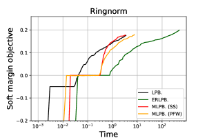
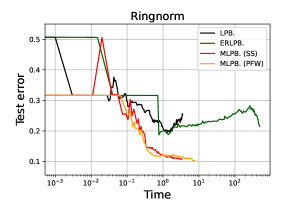
Figure 1: Comparison of the algorithm for the 0-th fold of Ringnorm dataset with parameters $\epsilon=0.01$ and $\nu=0.1m$. Left: soft margin objective value vs. computation time (seconds). Right: test error vs. computation time (seconds).

We compare LPBoost, ERLPBoost, and our scheme on Gunnar Rätsch’s benchmark dataset . We use a server with Intel Xeon Gold 6124 CPU 2.60GHz processors. We call our scheme with secondary Algorithm 2 as MLPBoost. MLPB. (SS) and MLPB. (PFW) are MLPBoosts with FW algorithms 3 and 4, respectively. The gradient boosting algorithms, like XGBoost (Chen and Guestrin, 2016) or LightGBM (Ke et al., 2017), solve different problems, so we do not compare our work to them. Note that the FW column corresponds to C-ERLPBoost.

In order to solve the sub-problems of LPBoost, ERLPBoost, and MLPBoost, we use the Gurobi optimizer 9.0.1 .

Settings.

We set the capping parameters $\nu\in N:=\{pm\mid p=0.1,0.2,\dots,0.5\}$ and the tolerance parameter $\epsilon=0.01$, where $m$ is the number of training instances. We use the weak learner that returns the best decision tree of depth 2.

Computation time.

We measure the CPU time and the System time using /usr/bin/time -v command. Some algorithms do not converge in a few days, so we abort the experiment by timeout 20000s command. We measure the running time with capping parameters over $N$ for each dataset and took their average. Table 2 shows the results. The FW column is the FW algorithm with short-steps, and PFW is the Pairwise FW algorithm. As the table shows, MLPB. (SS) and MLPB. (PFW) terminates much faster than FW and PFW, respectively. These results indicate that LPBoost rule $\mathcal{B}$, shown in Algorithm 2, significantly improves the objective. See the appendix for further comparisons.

Table 2: Comparison of the computation time (seconds). Each cell is the average computation time over the capping parameters over $N$. Some algorithm does not terminate in a few hours so we abort them within some appropriate time.

	Shape	LPB.	ERLPB.	MLPB. (SS only)	MLPB. (PFW only)	MLPB. (SS)	MLPB. (PFW)
Banana	$(5300,3)$	$168.26$	$3434.75$	$>10^{4}$	$>10^{4}$	$1418.41$	$1398.68$
B.Cancer	$(263,10)$	$3.61$	$73.45$	$180.16$	$270.50$	$23.43$	$19.81$
Diabetes	$(768,9)$	$47.53$	$1478.77$	$>10^{4}$	$3471.77$	$201.46$	$270.51$
F.Solar	$(144,10)$	$2.30$	$2.46$	$13.34$	$80.73$	$31.64$	$46.45$
German	$(1000,21)$	$77.56$	$1391.91$	$>10^{4}$	$5692.32$	$181.43$	$201.88$
Heart	$(270,14)$	$10.03$	$193.58$	$>10^{3}$	$183.09$	$44.11$	$24.26$
Image	$(2086,19)$	$8.25$	$107.52$	$>10^{3}$	$502.83$	$32.01$	$10.51$
R.norm	$(7400,21)$	$22.09$	$1148.16$	$>10^{4}$	$3350.87$	$26.76$	$36.73$
Splice	$(2991,61)$	$19.35$	$490.92$	$>10^{4}$	$943.98$	$122.08$	$37.88$
Thyroid	$(215,6)$	$0.70$	$0.66$	$367.51$	$0.35$	$2.71$	$0.61$
Titanic	$(24,4)$	$0.25$	$0.13$	$0.58$	$0.10$	$1.96$	$0.12$
Twonorm	$(7400,21)$	$105.40$	$13031.38$	$>10^{4}$	$989.54$	$478.22$	$397.91$
Waveform	$(5000,22)$	$437.29$	$9018.54$	$>10^{4}$	$>10^{4}$	$2243.07$	$1619.56$

The worst case for LPBoost.

Although LPBoost outperforms the running time in Table 2, it takes $m/2$ iterations for the worst case (Warmuth et al., 2007). Even in this case, MLPBoost and ERLPBoost terminate in 2 iterations.

Test errors.

For each dataset in the benchmark datasets, we first split them into train/test sets. Then, we perform the $5$-fold cross-validation over the training set, varying the capping parameter $\nu\in N$ to find the best one. Finally, train the algorithm using the whole training set with the best parameter and measure the test error with the test set. Table 3 summarizes the result. Since all the variants of MLPBoost solve the same problem, we only show MLPB. (SS) for comparison. As the table shows, MLPBoosts achieve small test errors for most datasets.

Table 3: Test errors for $5$-fold cross validation for the best parameters.

	LPB.	ERLPB.	MLPB. (SS)
Banana	0.28	0.37	0.10
B.Cancer	0.40	0.49	0.28
Diabetes	0.26	0.26	0.24
F.Solar	0.38	0.52	0.69
German	0.28	0.35	0.27
Heart	0.24	0.29	0.17
Image	0.10	0.20	0.02
Ringnorm	0.18	0.18	0.03
Splice	0.11	0.10	0.05
Thyroid	0.09	0.05	0.05
Titanic	0.60	0.60	0.60
Twonorm	0.03	0.04	0.03

6 Conclusion

We explored a relationship between the boosting algorithms for soft margin optimization and Frank-Wolfe algorithms via Fenchel duality. Using this unified view, we derived a scheme that can incorporate any secondary algorithm without losing the convergence guarantee. Even though our work is the fastest in the theoretically guaranteed boosting algorithms, LPBoost is still the fastest. We left the problem of inventing a faster boosting algorithm with a theoretical guarantee as future work.

Appendix A Technical lemmas and proofs

The following lemma shows the maximum value of the relative entropy from the uniform distribution over the capped probability simplex $\mathcal{P}^{m}_{\nu}$.

Lemma 3.

$\max_{\bm{d}\in\mathcal{P}^{m}_{\nu}}\Delta(\bm{d})\leq\ln\frac{m}{\nu}$.

Proof.

Since the relative entropy from the uniform distribution achieves its maximal value at the extreme points of $\mathcal{P}^{m}_{\nu}$, a maximizer has the form

$$\bm{d}=(\underbrace{1/\nu,1/\nu,\dots,1/\nu}_{k\text{ elements}},s,0,0,\dots,0),\quad s=1-\frac{k}{\nu}\leq\frac{1}{\nu}$$

for some $k\in[m]$. Plugging the maximizer into $\Delta(\bm{d})$, we can write the objective function as $\Delta(\bm{d})=(k/\nu)\ln(m/\nu)+s\ln(sm)$. If $s=0$, $\Delta(\bm{d})=\ln(m/\nu)$ holds since $k=\nu$. If $s>0$, $k/\nu<1$ so that

$$\Delta(\bm{d})\leq\frac{k}{\nu}\ln\frac{m}{\nu}+\left(1-\frac{k}{\nu}\right)\ln\frac{m}{\nu}=\ln\frac{m}{\nu}.$$

∎

Therefore, by setting $\eta=\frac{2}{\epsilon}\ln\frac{m}{\nu}$, the entropy term does not exceed $\frac{\epsilon}{2}$.

The following lemma shows the dual problem of the edge minimization.

Lemma 4.

Let $f:\mathbb{R}^{m}\to\{0,+\infty\}$, $g:\mathbb{R}^{n}\to\mathbb{R}$ be functions defined as

$$f(\bm{d})=\begin{cases}0&\bm{d}\in\mathcal{P}^{m}_{\nu}\\ +\infty&\bm{d}\notin\mathcal{P}^{m}_{\nu}\end{cases},\qquad\qquad\qquad g(\bm{\theta})=\max_{j\in[n]}\theta_{j}.$$

Then, the dual problem of edge minimization

$$\min_{\bm{d}}f(\bm{d})+g(A^{\top}\bm{d})$$ (20)

is the soft margin maximization

$$\max_{\bm{w}\in\mathcal{P}^{n}}-f^{\star}(-A\bm{w}).$$ (21)

Further, the strong duality holds.

Proof.

We can use Theorem 1 to derive the dual problem. Since

$$\bm{g}^{\star}(\bm{w})=\begin{cases}0&\bm{w}\in\mathcal{P}^{n}\\ +\infty&\bm{w}\notin\mathcal{P}^{n}\end{cases},$$

one can verify the dual form is given as (21). To prove the strong duality, it is enough to prove $\bm{0}\in\mathop{\rm int}\left(\mathop{\rm dom}g-A^{\top}\mathop{\rm dom}f\right)$. By definition, $\mathop{\rm dom}g=\mathbb{R}^{n}$ and $\mathop{\rm dom}f=\mathcal{P}^{m}_{\nu}$ and hence

$$\mathop{\rm dom}g-A^{\top}\mathop{\rm dom}f=\left\{\bm{w}-A^{\top}\bm{d}\mid\bm{w}\in\mathbb{R}^{n},\bm{d}\in\mathcal{P}^{m}_{\nu}\right\}.$$

Obviously, $\bm{0}\in\mathop{\rm int}(\mathop{\rm dom}g-A^{\top}\mathop{\rm dom}f)$ and thus the strong duality holds. ∎

Since

$$f^{\star}(-A\bm{w})=\sup_{\bm{d}}\left[-\bm{d}^{\top}A\bm{w}-f(\bm{d})\right]=\max_{\bm{d}\in\mathcal{P}^{m}_{\nu}}-\bm{d}^{\top}A\bm{w}=\min_{\bm{d}\in\mathcal{P}^{m}_{\nu}}\bm{d}^{\top}A\bm{w},$$

we can write the dual problem (21) explicitly:

$$\max_{\bm{w}\in\mathcal{P}^{n}}-f^{\star}(-A\bm{w})=-\min_{\bm{w}\in\mathcal{P}^{n}}\max_{\bm{d}\in\mathcal{P}^{m}_{\nu}}\bm{d}^{\top}A\bm{w}.$$

We get the dual problem for the regularized edge minimization problem by a similar derivation.

Corollary 2.

Let $f,g$ be the functions defined in Lemma 4 and let $\Delta(\bm{d})=\sum_{i=1}^{m}d_{i}\ln d_{i}+\ln(m)$ be the relative entropy function from the uniform distribution. Define $\tilde{f}=f+(1/\eta)\Delta$ for some $\eta>0$. Then, the dual problem of

$$\min_{\bm{d}}\tilde{f}(\bm{d})+g(A^{\top}\bm{d})\qquad\text{ is }\qquad\max_{\bm{w}\in\mathcal{P}^{n}}-\tilde{f}^{\star}(-A\bm{w}).$$

A.1 Proof of Lemma 1

Proof.

By the definition of Fenchel conjugate,

$$\tilde{f}^{\star}(\bm{\theta}) =\sup_{\bm{d}}\left\{\bm{d}^{\top}\bm{\theta}-\tilde{f}(\bm{d})\right\}\geq\sup_{\bm{d}}\left\{\bm{d}^{\top}\bm{\theta}-f(\bm{d})-c\right\}=f^{\star}(\bm{\theta})-c,$$

$$\tilde{f}^{\star}(\bm{\theta}) =\sup_{\bm{d}}\left\{\bm{d}^{\top}\bm{\theta}-\tilde{f}(\bm{d})\right\}\leq\sup_{\bm{d}}\left\{\bm{d}^{\top}\bm{\theta}-f(\bm{d})\right\}=f^{\star}(\bm{\theta}).$$

∎

By Lemma 3 and 1, we get $\tilde{f}^{\star}(-A\bm{w})-\frac{\epsilon}{2}\leq f(-A\bm{w})\leq\tilde{f}^{\star}(-A\bm{w})$ for all $-A\bm{w}$ if $\eta\geq\frac{2}{\epsilon}\ln\frac{m}{\nu}$.

A.2 Proof of Theorem 3 for the short-step FW rule 3

Recall that in the proof of Theorem 3, we showed the inequality $\epsilon_{t}-\epsilon_{t+1}\geq\frac{1}{8\eta}\epsilon_{t}^{2}$ for the short-step case. We prove $\epsilon_{t}\leq\frac{8\eta}{t+2}$ by induction on $t$. For the base case, $t=1$, by Lemma 1,

$$\epsilon_{1}=\min_{\tau\in\{0,1\}}(\bm{d}_{\tau}^{\top}A)_{j_{\tau+1}}+\tilde{f}^{\star}(-A\bm{w}_{1})\leq 1+f^{\star}(-A\bm{w}_{1})\leq 2\leq\frac{8\eta}{1+2}.$$

For the inductive case, assume that $\epsilon_{t}\leq\frac{8\eta}{t+2}$ for $t\geq 1$. By the inequality $\epsilon_{t}-\epsilon_{t+1}\geq\frac{1}{8\eta}\epsilon_{t}^{2}$, we have

$$\epsilon_{t+1}\leq\left(1-\frac{1}{8\eta}\epsilon_{t}\right)\epsilon_{t}.$$ (22)

By simple calculation, one can see that the maximizer $\epsilon$ of the RHS over $\mathbb{R}$ is $\epsilon=4\eta$. By the inductive assumption, $\epsilon_{t}\leq\frac{8\eta}{t+2}$. Since $\frac{8\eta}{t+2}$ is the maximizer of (22) over $[0,\frac{8\eta}{t+2}]$, we can plug this value into (22).

$$\epsilon_{t+1}\leq\left(1-\frac{1}{8\eta}\frac{8\eta}{t+2}\right)\frac{8\eta}{t+2}=\frac{t+1}{t+2}\frac{8\eta}{t+2}\leq\frac{8\eta}{t+3}$$

Therefore, $\epsilon_{t}\leq\frac{8\eta}{t+2}$ holds for all $t\geq 1$. Thus, we obtain the desired result.

Appendix B Additional experiments

This section includes experiments, not in the main paper. We first show the comparison of boosting algorithms, LPBoost, ERLPBoost, C-ERLPBoost, and our scheme. Since C-ERLPBoost is an instance of the short-step FW algorithm, we call it FW. We call our scheme with secondary algorithm 2 as MLPBoost. Figure 2 shows the convergence curve. MLPB. (SS) is MLPBoost with FW algorithm 3, and MLPB. (PFW) is MLPBoost with Pairwise FW algorithm 4. As expected, our algorithm converges faster than ERLPBoost and is competitive with LPBoost.

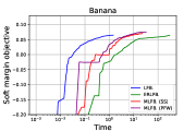
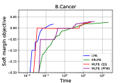
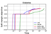
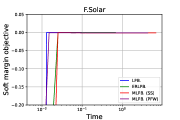
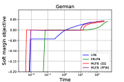
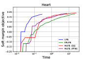
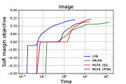
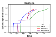
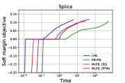
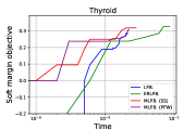
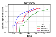
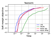
Figure 2: Time vs. soft margin objective with parameters $\nu=0.1m$ and $\epsilon=0.01$. Note that the time axis is log-scale. For many datasets, MLPBoosts tend to achieve a large margin rapidly.

Further, we compare the test error decrease. Figure 3 shows the test error curves. MLPB. (SS) achieves low test errors in most datasets.

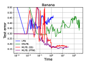
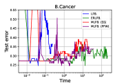
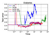
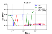
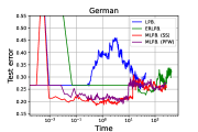
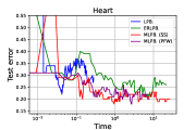
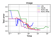
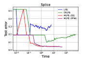
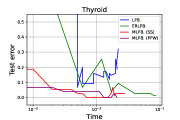
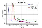
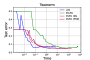
Figure 3: Time vs. test errors for the 0th fold of each dataset with parameters $\nu=0.1m$ and $\epsilon=0.01$. Note that the time axis is log-scale. For many datasets, MLPBoost tends to decrease the test error.

Now, we compare MLPBoosts to the Frank-Wolfe algorithms, FW and PFW. Figure 4 shows the number of $\mathcal{B}$ updates. This figure shows that the secondary update $\mathcal{B}$ yields better progress in early iterations. In the latter half, $\mathcal{F}$ yields better progress.

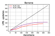
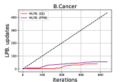
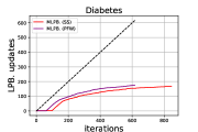
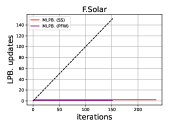
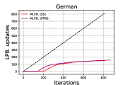
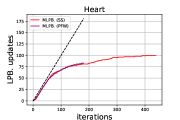
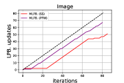
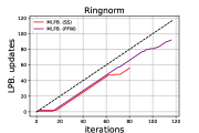
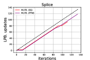
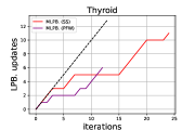
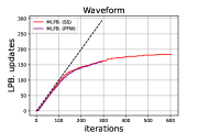
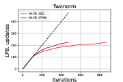
Figure 4: The number of $\mathcal{B}$ updates for each benchmark dataset with parameters $\nu=0.1m$ and $\epsilon=0.01$. The dotted line indicates the linear function for comparison. Since the shape of the titanic dataset is the same as the F. Solar dataset, we omit it.

Finally, we verify the effectiveness of the secondary update $\mathcal{B}$, shown in algorithm 2. For comparison, we measured the soft margin objective and time for FW, PFW, MLPB. (SS), and MLPB. (PFW). FW is the FW algorithm with short-steps, and PFW is the Pairwise FW algorithm. MLPB. (SS) and MLPB. (PFW) are MLPBoosts with algorithms 3 and 4, respectively. Figure 5 shows the results. As this figure shows, the secondary update $\mathcal{B}$ improves the objective value significantly.

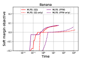
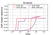
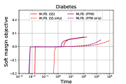
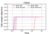
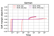
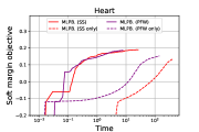
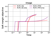
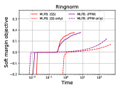
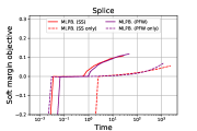
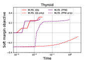
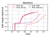
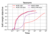
Figure 5: Comparison of the FW algorithms and MLPBoosts. As this figure shows, the secondary update $\mathcal{B}$ yields huge progress.

References

• Schapire et al. [1998] Robert E. Schapire, Yoav Freund, Peter Bartlett, and Wen Sun Lee. Boosting the margin: a new explanation for the effectiveness of voting methods. The Annals of Statistics, 26(5):1651–1686, 1998.
• Mohri et al. [2018] Mehryar Mohri, Afshin Rostamizadeh, and Amee Talwalker. Foundation of Machine Learning. The MIT Press, second edition, 2018.
• Demiriz et al. [2002] A Demiriz, K P Bennett, and J Shawe-Taylor. Linear Programming Boosting via Column Generation. Machine Learning, 46(1-3):225–254, 2002.
• Warmuth et al. [2007] M Warmuth, K Glocer, and G Rätsch. Boosting Algorithms for Maximizing the Soft Margin. In Advances in Neural Information Processing Systems 20 (NIPS 2007), pages 1585–1592, 2007.
• Shalev-Shwartz and Singer [2010] Shai Shalev-Shwartz and Yoram Singer. On the equivalence of weak learnability and linear separability: new relaxations and efficient boosting algorithms. Mach. Learn., 80(2-3), 2010.
• Warmuth et al. [2008] Manfred K. Warmuth, Karen A. Glocer, and S. V. N. Vishwanathan. Entropy regularized lpboost. In Algorithmic Learning Theory, 19th International Conference, ALT 2008, Budapest, Hungary, October 13-16, 2008. Proceedings, volume 5254 of Lecture Notes in Computer Science, pages 256–271. Springer, 2008.
• Borwein and Lewis [2006] Jonathan M. Borwein and Adrian S. Lewis. Convex Analysis, pages 65–96. Springer New York, 2006.
• Frank and Wolfe [1956] Marguerite Frank and Philip Wolfe. An algorithm for quadratic programming. Naval Research Logistics Quarterly, 3(1-2):95–110, 1956.
• Jaggi [2013] Martin Jaggi. Revisiting frank-wolfe: Projection-free sparse convex optimization. In Proceedings of the 30th International Conference on Machine Learning, ICML 2013, volume 28 of JMLR Workshop and Conference Proceedings, pages 427–435. JMLR.org, 2013.
• Wang et al. [2015] Chu Wang, Yingfei Wang, E Weinan, and Robert E. Schapire. Functional frank-wolfe boosting for general loss functions. ArXiv, abs/1510.02558, 2015.
• Herbster and Warmuth [2001] Mark Herbster and Manfred K. Warmuth. Tracking the best linear predictor. J. Mach. Learn. Res., 1:281–309, sep 2001.
• Lacoste-Julien and Jaggi [2015] Simon Lacoste-Julien and Martin Jaggi. On the global linear convergence of frank-wolfe optimization variants. In Advances in Neural Information Processing Systems 28: Annual Conference on Neural Information Processing Systems 2015, December 7-12, 2015, Montreal, Quebec, Canada, pages 496–504, 2015.
• Chen and Guestrin [2016] Tianqi Chen and Carlos Guestrin. Xgboost: A scalable tree boosting system. In Proceedings of the 22nd ACM SIGKDD International Conference on Knowledge Discovery and Data Mining, KDD ’16, page 785–794. Association for Computing Machinery, 2016.
• Ke et al. [2017] Guolin Ke, Qi Meng, Thomas Finley, Taifeng Wang, Wei Chen, Weidong Ma, Qiwei Ye, and Tie-Yan Liu. Lightgbm: A highly efficient gradient boosting decision tree. In Isabelle Guyon, Ulrike von Luxburg, Samy Bengio, Hanna M. Wallach, Rob Fergus, S. V. N. Vishwanathan, and Roman Garnett, editors, Advances in Neural Information Processing Systems 30: Annual Conference on Neural Information Processing Systems 2017, December 4-9, 2017, Long Beach, CA, USA, pages 3146–3154, 2017.