Nonsmooth Nonconvex-Nonconcave Minimax Optimization: Primal-Dual Balancing and Iteration Complexity Analysis

Abstract

Nonconvex-nonconcave minimax optimization has gained widespread interest over the last decade. However, most existing works focus on variants of gradient descent-ascent (GDA) algorithms, which are only applicable to smooth nonconvex-concave settings. To address this limitation, we propose a novel algorithm named smoothed proximal linear descent-ascent (smoothed PLDA), which can effectively handle a broad range of structured nonsmooth nonconvex-nonconcave minimax problems. Specifically, we consider the setting where the primal function has a nonsmooth composite structure and the dual function possesses the Kurdyka-Łojasiewicz (KŁ) property with exponent $\theta\in[0,1)$. We introduce a novel convergence analysis framework for smoothed PLDA, the key components of which are our newly developed nonsmooth primal error bound and dual error bound. Using this framework, we show that smoothed PLDA can find both $\epsilon$-game-stationary points and $\epsilon$-optimization-stationary points of the problems of interest in $\mathcal{O}(\epsilon^{-2\max\{2\theta,1\}})$ iterations. Furthermore, when $\theta\in[0,\frac{1}{2}]$, smoothed PLDA achieves the optimal iteration complexity of $\mathcal{O}(\epsilon^{-2})$. To further demonstrate the effectiveness and wide applicability of our analysis framework, we show that certain max-structured problem possesses the KŁ property with exponent $\theta=0$ under mild assumptions. As a by-product, we establish algorithm-independent quantitative relationships among various stationarity concepts, which may be of independent interest.

Keywords: Nonconvex-Nonconcave Minimax Optimization, Proximal Linear Scheme, Nonsmooth Composite Structure, Perturbation Analysis, Kurdyka-Łojasiewicz Property

1 Introduction

In this paper, we aim to solve the following minimax problem:

$$\min_{x\in\mathcal{X}}\max_{y\in\mathcal{Y}}F(x,y).$$ (P)

Here, $F:\mathbb{R}^{n}\times\mathbb{R}^{d}\rightarrow\mathbb{R}$ can be both nonconvex with respect to $x$ and nonconcave with respect to $y$, $\mathcal{X}\subseteq\mathbb{R}^{n}$ is a nonempty closed convex set, and $\mathcal{Y}\subseteq\mathbb{R}^{d}$ is a nonempty compact convex set. This problem has a wide range of applications in machine learning and operations research. Examples include learning with non-decomposable loss (Zhang and Zhou,, 2018; Shalev-Shwartz and Wexler,, 2016), training generative adversarial networks (Goodfellow et al.,, 2020; Arjovsky et al.,, 2017), adversarial training (Madry et al.,, 2018; Sinha et al.,, 2018), and (distributionally) robust optimization (DRO) (Bertsimas et al.,, 2011; Rahimian and Mehrotra,, 2022).

When $F$ is a smooth function, a natural and intuitive approach for solving (P) is gradient descent-ascent (GDA), which involves performing gradient descent on the primal variable $x$ and gradient ascent on the dual variable $y$ in each iteration. For nonconvex-strongly concave problems, GDA can find an $\epsilon$-stationary point with an iteration complexity of ${\mathcal{O}}(\epsilon^{-2})$ (Lin et al., 2020b, ). This matches the lower bound for solving (P) using a first-order oracle, as shown in (Carmon et al.,, 2020; Zhang et al.,, 2021; Li et al.,, 2021). However, when $F(x,\cdot)$ is not strongly concave for some $x\in\mathcal{X}$, GDA may encounter oscillations, even for bilinear problems. To overcome this challenge, various techniques utilizing diminishing step sizes have been proposed to guarantee convergence. Nevertheless, these techniques can only achieve a suboptimal complexity of ${\mathcal{O}}(\epsilon^{-6})$ at best (Lu et al.,, 2020; Lin et al., 2020b, ; Jin et al.,, 2020). To achieve a lower iteration complexity, the works (Zhang et al.,, 2020; Xu et al.,, 2023) introduce a smoothing technique to stabilize the iterates. As a result, the complexity is improved to ${\mathcal{O}}(\epsilon^{-4})$ for general nonconvex-concave problems. Moreover, the works (Zhang et al.,, 2020; Yang et al.,, 2022) achieve the “optimal” iteration complexity of $\mathcal{O}(\epsilon^{-2})$ for dual functions that either take a pointwise-maximum form or possess the Polyak-Łojasiewicz (PŁ) property (Polyak,, 1963). On another front, multi-loop-type algorithms have been developed to achieve a lower iteration complexity for general nonconvex-concave problems (Yang et al.,, 2020; Ostrovskii et al.,, 2021; Nouiehed et al.,, 2019; Thekumparampil et al.,, 2019). Among these, the two triple-loop algorithms in (Lin et al., 2020a, ; Ostrovskii et al.,, 2021) have the lowest iteration complexity of $\mathcal{O}(\epsilon^{-2.5})$.

If we take one step into the nonsmooth world with (P) possessing a separable nonsmooth structure, i.e., its objective function consists of a smooth term and a separable nonsmooth term whose proximal mapping can be readily computed, then the analytic and algorithmic framework from the purely smooth case can be easily adapted. Specifically, a class of (accelerated) proximal-GDA type algorithms have been proposed, where the gradient step is substituted by the proximal gradient step (Huang et al.,, 2021; Barazandeh and Razaviyayn,, 2020; Chen et al.,, 2021; Boţ and Böhm,, 2020). By utilizing the gradient Lipschitz continuity condition of the smooth term, these algorithms can be shown to achieve the same iteration complexity as those for the smooth case.

As we can see, most existing algorithms can only handle the almost smooth case, which refers to scenarios where at least some gradient information is obtainable, such as in purely smooth or separable nonsmooth problems. By contrast, the general nonsmooth problem has received relatively little attention in the minimax literature. Only recently have two algorithms, namely the proximally guided stochastic subgradient method (Rafique et al.,, 2022) and two-timescale GDA (Lin et al.,, 2022), been proposed to tackle general nonsmooth weakly convex-concave problems. Unfortunately, these methods suffer from the high iteration complexities of $\mathcal{O}(\epsilon^{-6})$ and $\mathcal{O}(\epsilon^{-8})$, respectively, since they only use subgradient information and neglect problem-specific structures. Thus, a natural question arises: Q1: Are there structured nonsmooth nonconvex-nonconcave problems whose $\epsilon$-stationary points can be found with an iteration complexity of $\mathcal{O}(\epsilon^{-4})$, just like smooth nonconvex-concave problems? Taking a step further, we would like to pose a more challenging and intriguing question: Q2: Can we identify general regularity conditions to achieve the “optimal” rate of $\mathcal{O}(\epsilon^{-2})$ for nonsmooth nonconvex-nonconcave problems?

1.1 Main Contributions

This paper provides affirmative answers to both questions Q1 and Q2 for a particular class of nonsmooth nonconvex-nonconcave problems. We focus on a primal function that has the composite structure $F(\cdot,y):=h_{y}\circ c_{y}$ for each $y\in\mathcal{Y}$, where $h_{y}$ is convex, Lipschitz continuous, and possibly nonsmooth; $c_{y}$ is continuously differentiable with a Lipschitz continuous Jacobian map; and the dual function is continuously differentiable and gradient Lipschitz continuous on $\mathcal{X}\times\mathcal{Y}$. Additionally, we assume that the dual function either possesses the KŁ property with exponent $\theta\in[0,1)$ or is a general concave function. As concavity alone cannot guarantee the KŁ property (Bolte et al.,, 2010), we deal with the general concave case separately.

To start, we introduce a new algorithm called smoothed proximal linear descent-ascent (smoothed PLDA), which builds on the smoothed GDA algorithm (Zhang et al.,, 2020). Unlike its predecessor, smoothed PLDA is extended to handle nonsmooth composite nonconvex-nonconcave problems. To achieve this, we leverage the proximal linear scheme to effectively manage the nonsmooth composite structure of the primal function. This scheme has been extensively studied in recent literature (Nesterov,, 2007; Cartis et al.,, 2011; Lewis and Wright,, 2016; Hu et al.,, 2016; Drusvyatskiy and Lewis,, 2018; Drusvyatskiy and Paquette,, 2019; Hu et al.,, 2023), though its application to minimax optimization has not been explored.

Although the algorithmic extension may seem intuitive and straightforward, it introduces notable challenges in the convergence analysis. These challenges arise primarily from the lack of gradient Lipschitz continuity of the primal function and the nonconcavity of the dual function. To address these challenges, we first establish a tight Lipschitz-type primal error bound property of the proximal linear scheme, which holds even without the gradient Lipschitz continuity condition (see Proposition 2). This error bound is new and plays a crucial role in demonstrating the sufficient decrease property of the designed Lyapunov function. The sufficient decrease property serves as a starting point to ensure the global convergence of smoothed PLDA.

Next, we observe that the nonconcavity of the dual function poses a fundamental challenge in achieving a favorable tradeoff between the decrease in the primal and the increase in the dual. This challenge arises from the absence of inherent dominance between the primal and dual functions, making it difficult to find an optimal balance between the primal and dual updates. As it turns out, the primal-dual tradeoff directly impacts the convergence rate. To quantify this tradeoff, we introduce a new dual error bound property based on the KŁ exponent of the dual function (see Proposition 3). This is a notable departure from the usual approach of utilizing the KŁ exponent in pure primal nonconvex optimization (Li and Pong,, 2018; Attouch et al.,, 2013).

Table 1: Comparison of the iteration complexities of smoothed PLDA and other related methods under different settings for solving $\min_{x\in\mathcal{X}}\max_{y\in\mathcal{Y}}F(x,y)$.

The aforementioned primal and dual error bounds lie at the core of our convergence analysis framework. Our main result is that, when the dual function possesses the KŁ property with exponent $\theta\in[0,1)$, smoothed PLDA can find both $\epsilon$-game-stationary points and $\epsilon$-optimization-stationary points of the nonsmooth composite nonconvex-nonconcave problems introduced earlier in $\mathcal{O}(\epsilon^{-2\max\{2\theta,1\}})$ iterations. For general concave functions, smoothed PLDA attains the same iteration complexity of $\mathcal{O}(\epsilon^{-4})$ as the smoothed GDA in (Zhang et al.,, 2020). Therefore, we address Q1 by extending smoothed GDA to a nonsmooth nonconvex-nonconcave setting while preserving at least the same iteration complexity. Table 1 presents a summary of the iteration complexities of smoothed PLDA and other related methods in various scenarios. Using our analysis framework, we further show that when the KŁ exponent of the dual function lies between 0 and $\frac{1}{2}$, smoothed PLDA achieves the “optimal” iteration complexity of $\mathcal{O}(\epsilon^{-2})$, thus addressing Q2.

Interestingly, our analysis framework also reveals a phase transition phenomenon: The iteration complexity depends on the slower of the primal and dual variable updates, which can be characterized by the dual error bound. Specifically, when $\theta\in[0,\frac{1}{2}]$, the dual update is faster than the primal update, which causes the primal update to dominate the optimization process. However, since the primal update involves solving a strongly convex problem, we cannot achieve an iteration complexity better than $\mathcal{O}(\epsilon^{-2})$, which is optimal for nonconvex-strongly concave problems. By contrast, when $\theta\in(\frac{1}{2},1)$, the dual update dominates, and the iteration complexity explicitly depends on the KŁ exponent $\theta$, i.e., $\mathcal{O}(\epsilon^{-4\theta})$.

To further demonstrate the wide applicability and effectiveness of our analysis framework, we apply it to problems with a linear dual function and polytopal constraints on $y$. An important example is the max-structured problem, which takes the form

$$\min_{x\in\mathcal{X}}\max_{i\in[d]}G_{i}(x).$$ (1.1)

Here, $G_{i}:\mathbb{R}^{n}\rightarrow\mathbb{R}$, where $i\in[d]$, is a nonconvex function with the composite structure mentioned earlier. Such a problem arises frequently in machine learning applications, including distributionally robust optimization (DRO) (Gao et al.,, 2022; Shafieezadeh-Abadeh et al.,, 2019; Blanchet et al., 2019a, ), adversarial training (Madry et al.,, 2018), fairness training (Nouiehed et al.,, 2019; Mohri et al.,, 2019), and distribution-agnostic meta-learning (Collins et al.,, 2020). Under some regularity conditions, we show that problem (1.1) possesses the KŁ property with exponent $\theta=0$.

Finally, the new dual error bound enables us to establish algorithm-independent quantitative relationships among different stationarity concepts (see Theorem 3). The relationships are obtained as a by-product of our analysis and extend the scope of previous results in (Jin et al.,, 2020; Razaviyayn et al.,, 2020; Daskalakis et al.,, 2021) to a wider range of settings. Furthermore, they hold great promise for demystifying various notions of stationarity in the context of minimax optimization.

Structure of the paper

The paper is organized as follows. In Section 2, we provide several representative applications to demonstrate not only the prevalence of problem (P) when the primal function $F$ has the composite structure mentioned earlier but also the versatility of our proposed smoothed PLDA. In Section 3, we introduce the problem setup and key concepts used throughout the paper. We then present our proposed algorithm and a new convergence analysis framework for studying it in Sections 4 and 5, respectively. In Section 6, we verify that the max-structured problem (1.1) possesses the KŁ property with exponent $\theta=0$. In Section 7, we clarify the relationships among various stationarity concepts, both conceptually and quantitatively. Finally, we end with some closing remarks in Section 8.

2 Motivating Applications

One important class of problems that is mostly beyond the reach of existing algorithmic approaches but can be tackled by our proposed smoothed PLDA is “two-layer” nonsmooth composite optimization, which takes the form

$$\min_{x\in\mathcal{X}}f(h(c(x))).$$ (2.1)

Here, $f:\mathbb{R}^{d}\rightarrow\mathbb{R}$ is convex, $h:\mathbb{R}^{m}\rightarrow\mathbb{R}^{d}$ is convex and Lipschitz continuous, and $c:\mathbb{R}^{n}\rightarrow\mathbb{R}^{m}$ is continuously differentiable with a Lipschitz continuous Jacobian map. Note that both $f$ and $h$ can be nonsmooth. Now, observe that we can isolate the first-layer nonsmoothness by reformulating (2.1) as the minimax problem

$$\min_{x\in\mathcal{X}}\max_{y\in\mathbb{R}^{d}}y^{\top}h(c(x))-f^{\star}(y),$$ (2.2)

where $f^{\star}:\mathbb{R}^{d}\rightarrow\mathbb{R}\cup\{+\infty\}$ is the conjugate function of $f$. Consequently, we can apply our proposed smoothed PLDA to solve (2.2).

Various applications admit formulations that feature the nonsmooth composite structure in (2.1). Let us discuss two representative ones here.

(i) Variation-Regularized Wasserstein DRO (Gao et al.,, 2022)

The DRO methodology aims to find optimal decisions under the most adverse distribution in an ambiguity set, which consists of all probability distributions that fit the observed data with high confidence. In recent years, several works have interpreted regularization from a DRO perspective; see, e.g., (Rahimian and Mehrotra,, 2022; Blanchet et al., 2019b, ; Gao et al.,, 2022; Shafieezadeh-Abadeh et al.,, 2019; Namkoong and Duchi,, 2016; Cranko et al.,, 2021). These works provide a probabilistic justification for existing regularization techniques and offer an alternative approach to tackle risk minimization problems. For instance, the work Gao et al., (2022) establishes the asymptotic equivalence between Wasserstein distance-induced DRO and the following variation-regularized problem:

$$\min_{\theta\in\Theta}\,\frac{1}{N}\sum_{i=1}^{N}\ell(f_{\theta}(x_{i}),y_{i})+\rho\max_{i\in[N]}\|\nabla_{x}f_{\theta}(x_{i})\|_{q}.$$ (2.3)

Here, $\{(x_{i},y_{i})\}_{i\in[N]}$ are the feature-label pairs, $\ell:\mathbb{R}\rightarrow\mathbb{R}$ is the loss function, $f_{\theta}$ is the feature mapping (e.g., a neural network parameterized by $\theta$), $\rho>0$ is the constraint radius, and $q\in[1,+\infty]$ is a parameter. The variation regularization can be regarded as an empirical alternative to Lipschitz regularization, where the goal is to promote smoothness of $f_{\theta}$ over the entire training dataset. Since problem (2.3) is closely related to the task of controlling the Lipschitz constant of deep neural networks, it has attracted significant interest. In particular, problem (2.3) with $\ell(\cdot)=|\cdot|$ being the absolute loss and $f_{\theta}$ being a linear mapping is thoroughly investigated in (Blanchet et al., 2019a, ).

(ii) $\ell_{1}$-Regression with Heavy-Tailed Distributions (Zhang and Zhou,, 2018)

In linear regression, when the input and output follow heavy-tailed distributions, empirical risk minimization may no longer be a suitable approach. This observation has led to recent research on learning with heavy-tailed distributions (Audibert and Catoni,, 2011). For instance, the work Zhang and Zhou, (2018) proposes the following truncated minimization problem for $\ell_{1}$-regression with heavy-tailed distributions:

$$\min_{\theta\in\Theta}\,\frac{1}{\alpha N}\sum_{i=1}^{N}\psi\left(\alpha|y_{i}-\theta^{\top}x_{i}|\right).$$ (2.4)

Here, $\alpha>0$ is a parameter and $\psi:\mathbb{R}\rightarrow\mathbb{R}$ is the nondecreasing truncation function defined by

$$\psi(t)=\begin{cases}&\log\left(1+t+\frac{t^{2}}{2}\right),\quad t\geq 0\\ &-\log\left(1-t+\frac{t^{2}}{2}\right),\quad t\leq 0.\end{cases}$$

Note that $\psi$ is a $\frac{1}{4}$-weakly convex function. Then, problem (2.4) can be reformulated as

$$\min_{\theta\in\Theta}\max_{q\in\mathbb{R}^{N}}\frac{1}{\alpha N}\sum_{i=1}^{N}\left[\alpha q_{i}|y_{i}-\theta^{\top}x_{i}|-\psi^{\star}_{\mu}(q_{i})-\frac{\mu\alpha^{2}}{2}\|y_{i}-\theta^{\top}x_{i}\|^{2}\right],$$

where $\psi_{\mu}(\cdot)=\psi(\cdot)+\frac{\mu}{2}\|\cdot\|^{2}$ and $\mu>\frac{1}{4}$ so as to enforce the strong convexity of $\psi_{\mu}$. To the best of our knowledge, there is no provably efficient algorithm for solving (2.4).

Besides the nonsmooth composite optimization problem (2.1), a variety of minimax problems can also be tackled by smoothed PLDA. Let us illustrate this by considering the general $\phi$-divergence DRO problem studied in (Levy et al.,, 2020).

(iii) General $\phi$-Divergence DRO (Levy et al.,, 2020)

Building on the problem setup in (i), we consider a slight generalization of $\phi$-divergence DRO, which is given by

$$\min_{\theta\in\Theta}\max_{q\in\Delta_{N}:\sum_{i=1}^{N}\phi(Nq_{i})\leq n\rho}\frac{1}{N}\sum_{i=1}^{N}q_{i}\ell(f_{\theta}(x_{i},y_{i}))-\psi(Nq_{i}).$$ (2.5)

Here, the functions $\phi,\psi:\mathbb{R}\rightarrow\mathbb{R}$ are convex and satisfy $\phi(1)=\psi(1)=0$, $\rho\geq 0$ is the constraint radius, and $\Delta_{N}$ is the $N$-dimensional standard simplex. When $\phi=0$ and $\psi=\iota_{[0,1/\alpha)}$ with $\alpha\in[0,1)$, problem (2.5) reduces to Conditional Value-at-Risk minimization (Rockafellar and Uryasev,, 2000). When $\psi=0$ and $\phi(t)=t\log t-t+1$, problem (2.5) reduces to Kullback-Leibler divergence DRO (Hu and Hong,, 2013). While the algorithmic approach in (Levy et al.,, 2020) only applies to the case where $\ell$ and $f_{\theta}$ are both smooth, our proposed smoothed PLDA is able to handle a wide range of loss functions, including nonsmooth losses such as the absolute loss.

3 Preliminaries

Let us introduce the basic problem setup and key concepts that will serve as the basis for our subsequent analysis.

Assumption 1 (Problem setup).

The following assumptions on the objective function $F$ of problem (P) hold throughout the paper.

1. $(\textrm{\bf Primal function})$ For all $y\in\mathcal{Y}$, the function $F(\cdot,y):\mathbb{R}^{n}\rightarrow\mathbb{R}$ takes the form $F(\cdot,y):=h_{y}\circ c_{y}$, where $c_{y}:\mathbb{R}^{n}\rightarrow\mathbb{R}^{m}$ is continuously differentiable with $L_{c}$-Lipschitz continuous Jacobian map, i.e.,

   $$\|\nabla c_{y}(x)-\nabla c_{y}(x^{\prime})\|\leq L_{c}\|x-x^{\prime}\|\quad\text{ for all }x,x^{\prime}\in\mathcal{X};$$

   and $h_{y}:\mathbb{R}^{m}\rightarrow\mathbb{R}$ is convex and $L_{h}$-Lipschitz continuous, i.e.,

   $$|h_{y}(z)-h_{y}(z^{\prime})|\leq L_{h}\|z-z^{\prime}\|\quad\text{ for all }z,z^{\prime}\in\mathbb{R}^{m}.$$

2. $(\textrm{\bf Dual function})$ For all $x\in\mathcal{X}$, the function $F(x,\cdot):\mathbb{R}^{d}\rightarrow\mathbb{R}$ is continuously differentiable with $\nabla_{y}F(\cdot,\cdot)$ being $L$-Lipschitz continuous on $\mathcal{X}\times\mathcal{Y}$, i.e.,

   $$\|\nabla_{y}F(x,y)-\nabla_{y}F(x^{\prime},y^{\prime})\|\leq L\|(x,y)-(x^{\prime},y^{\prime})\|\,\text{ for all }(x,y),(x^{\prime},y^{\prime})\in\mathcal{X}\times\mathcal{Y}.$$

   Without loss of generality, we may take $L=L_{h}L_{c}$.

Assumption 2 (KŁ property with exponent $\theta$ for dual function).

For all $x\in\mathcal{X}$, the problem $\max_{y\in\mathcal{Y}}F(x,y)$ has a nonempty solution set and a finite optimal value. Moreover, there exist $\mu>0$ and $\theta\in[0,1)$ such that

$$\operatorname{dist}(0,-\nabla_{y}F(x,y)+\partial\iota_{\mathcal{Y}}(y))\geq\mu\left(\max\limits_{y^{\prime}\in\mathcal{Y}}F(x,y^{\prime})-F(x,y)\right)^{\theta}$$

for all $x\in\mathcal{X}$ and $y\in\mathcal{Y}$.

Remark 1.

The PŁ property has been widely used as a standard assumption in nonconvex-nonconcave minimax optimization (Nouiehed et al.,, 2019; Yang et al.,, 2022). However, its usage is restricted to smooth unconstrained settings. To overcome this limitation, we employ the KŁ property, which has been demonstrated in (Attouch et al.,, 2010) to be a nonsmooth extension of the PŁ property. The KŁ exponent, a crucial quantity in the convergence rate analysis of first-order methods for nonconvex optimization (Li and Pong,, 2018; Frankel et al.,, 2015), plays a vital role in establishing the explicit convergence rate of smoothed PLDA.

Let us now examine the stationarity measures discussed in this paper. We define the value function $f:\mathbb{R}^{n}\rightarrow\mathbb{R}$, the potential function $F_{r}:\mathbb{R}^{n}\times\mathbb{R}^{d}\times\mathbb{R}^{n}\rightarrow\mathbb{R}$, and the dual function $d_{r}:\mathbb{R}^{d}\times\mathbb{R}^{n}\rightarrow\mathbb{R}$ by

$$f(x) :=\max_{y\in\mathcal{Y}}F(x,y),$$

$$F_{r}(x,y,z) :=F(x,y)+\frac{r}{2}\|x-z\|^{2},$$

$$d_{r}(y,z) :=\min_{x\in\mathcal{X}}F_{r}(x,y,z),$$

respectively, where we assume $r>L$ in the rest of this paper.

As the function $F(\cdot,y)$ is weakly convex for each $y\in\mathcal{Y}$, the value function $f$ is also weakly convex. Thus, motivated by the development in (Davis and Drusvyatskiy,, 2019), we may use the measure in Definition 1(a), which we call optimization stationarity, as a (primal) stationarity measure for (P). On the other hand, observe that $\nabla_{z}d_{r}(y,x)=r(x-\operatorname{prox}_{\frac{1}{r}F(\cdot,y)+\iota_{\mathcal{X}}}(x))$ by Danskin’s theorem. Here, $\operatorname{prox}$ denotes the proximal mapping; see Definition 4 in Appendix A. Thus, we may use the measure in Definition 1(b), which we call game stationarity, as a (primal-dual) stationarity measure for (P).

Definition 1 (Stationarity measures).

Let $\epsilon\geq 0$ be given.

1. The point $x\in\mathcal{X}$ is an $\epsilon$-optimization-stationary point ($\epsilon$-OS) of problem (P) if

   $$\|\operatorname{prox}_{\frac{1}{r}f+\iota_{\mathcal{X}}}(x)-x\|\leq\epsilon.$$

2. The pair $(x,y)\in\mathcal{X}\times\mathcal{Y}$ is an $\epsilon$-game-stationary point ($\epsilon$-GS) of problem (P) if

   $$\|\nabla_{z}d_{r}(y,x)\|\leq\epsilon\quad\text{and}\quad{\rm dist}(0,-\nabla_{y}F(x,y)+\partial\iota_{\mathcal{Y}}(y))\leq\epsilon.$$

Since weakly convex functions and smooth functions are subdifferentially regular, we can utilize the Fréchet subdifferential in the above definitions. A brief overview of various subdifferential constructions in nonsmooth nonconvex optimization can be found in (Li et al.,, 2020). In Section 7, we will explore the quantitative relationship between the two stationarity measures in Definition 1.

4 Proposed Algorithm — Smoothed PLDA

GDA is a commonly used method for solving smooth nonconvex-concave problems. However, its vanilla implementation can lead to oscillations, and a conventional approach to mitigate this issue is to use diminishing step sizes. Unfortunately, one cannot achieve the optimal iteration complexity with this approach. In view of this, the work (Zhang et al.,, 2020) proposes a Nesterov-type smoothing technique that stabilizes the primal sequence and achieves a better balance between primal and dual updates. However, the technique crucially relies on the smoothness of the objective function.

The nonsmoothness in our problem setting poses a key challenge to algorithm design. To overcome this challenge, we fully leverage the composite structure of the primal function and adopt the proximal linear scheme for the primal update (Drusvyatskiy and Paquette,, 2019). Specifically, given $r>L$ and $\lambda>0$, consider the update

$$x^{k+1}\in\mathop{\operatorname*{argmin}}_{x\in\mathcal{X}}\left\{F_{x^{k},\lambda}(x,y^{k})+\frac{r}{2}\|x-z^{k}\|^{2}\right\},$$ (4.1)

where

$$F_{x^{k},\lambda}(x,y^{k}):=h_{y^{k}}\left(c_{y^{k}}(x^{k})+\nabla c_{y^{k}}(x^{k})^{\top}(x-x^{k})\right)+\frac{1}{2\lambda}\|x-x^{k}\|^{2}.$$

Here, $\{z^{k}\}$ is an auxiliary sequence. In particular, when $h(t)=t$, the primal update (4.1) reduces to the standard gradient descent step as described in (Zhang et al.,, 2020). The dual update and other smoothing steps are the same as those in the smoothed GDA developed in (Zhang et al.,, 2020).

Our smoothed PLDA algorithm is formally presented in Algorithm 1.

Input : Initial point $(x^{0},y^{0},z^{0})$ and parameters $r>L$, $\lambda>0$, $\alpha>0$, $\beta\in(0,1)$

1 for $k=0,1,2,\ldots$ do

2       $x^{k+1}:=\mathop{\operatorname*{argmin}}\limits_{x\in\mathcal{X}}\left\{F_{x^{k},\lambda}(x,y^{k})+\frac{r}{2}\|x-z^{k}\|^{2}\right\}$

3       $y^{k+1}:=\operatorname{proj}_{\mathcal{Y}}\left(y^{k}+\alpha\nabla_{y}F(x^{k+1},y^{k})\right)$

4       $z^{k+1}:=z^{k}+\beta(x^{k+1}-z^{k})$

5 end for

Algorithm 1 Smoothed PLDA

Remark 2 (Primal update).

Finding a closed-form solution for the primal update (4.1) is challenging due to the nonsmooth composite structure. However, problem (4.1) is strongly convex, which means that an $\epsilon$-optimal solution can be found by, e.g., proximal gradient methods in at most $\mathcal{O}(\log(\frac{1}{\epsilon}))$ iterations (Bubeck,, 2015, Theorem 3.15). It is important to note that the lower bound on the iteration complexity of first-order methods for solving nonsmooth strongly convex problems is $\Omega(1/\epsilon^{2})$ (Bubeck,, 2015, Theorem 3.13). We would like to highlight that the optimal approach to solving (4.1) depends on the problem’s specific structure. For simplicity and to focus on our main contributions, we assume the exactness of the primal update and concentrate on the iteration complexity of the outer loop in subsequent analyses.

5 Convergence Analysis of Smoothed PLDA

In this section, we present the main theoretical contributions of this paper. Our goal is to investigate the convergence rate of smoothed PLDA (see Theorem 1) under different settings, including nonconvex-KŁ and nonconvex-concave.

Before proceeding, let us fix the notation as in Table 2.

Table 2: Notation

5.1 Analysis Framework

We start by presenting the key ideas in the analysis.

Building on (Zhang et al.,, 2020), we define the Lyapunov function $\Phi_{r}:\mathbb{R}^{n}\times\mathbb{R}^{d}\times\mathbb{R}^{n}\rightarrow\mathbb{R}$ as follows:

$$\Phi_{r}(x,y,z):=\underbrace{F_{r}(x,y,z)-d_{r}(y,z)}_{\textnormal{Primal Descent}}+\underbrace{p_{r}(z)-d_{r}(y,z)}_{\textnormal{Dual Ascent}}+\underbrace{p_{r}(z)}_{\textnormal{Proximal Descent}}.$$

The sole distinction between the above Lyapunov function and the one in (Zhang et al.,, 2020) is that we swap the order of min and max in the definition of $p_{r}$, transitioning from $\min_{x\in\mathcal{X}}\max_{y\in\mathcal{Y}}F_{r}(x,y,\cdot)$ to $\max_{y\in\mathcal{Y}}\min_{x\in\mathcal{X}}F_{r}(x,y,\cdot)$. This alteration enables a more comprehensive analysis of cases where the dual function is nonconcave. Each term in the potential function $\Phi_{r}$ is tightly connected to the algorithmic updates. Specifically, the updates for the primal, dual, and auxiliary variables can be viewed as a descent step on the primal function $F_{r}$, an approximate ascent step on the dual function $d_{r}$, and an approximate descent step on the proximal function $p_{r}$, respectively.

Next, our task is to quantify the change in each term of the Lyapunov function after one round of updates. To do so, the key step is the following:

Intuitively, the primal error bound provides an estimate of the distance between the current point $x^{k+1}$ and the optimal solution

$$x_{r}(y_{k},z_{k})=\mathop{\operatorname*{argmin}}\limits_{x\in\mathcal{X}}F_{r}(x,y_{k},z_{k})$$

in terms of the iterates gap $\|x^{k+1}-x^{k}\|$ that results from the proximal linear scheme.

Equipped with the primal error bound, we can obtain the following basic descent estimate of the Lyapunov function:

Proposition 1 (Basic descent estimate of $\Phi_{r}$).

Let

$$r\geq 3L,\ \lambda\leq\frac{1}{L},\ \alpha\leq\min\left\{\frac{1}{10L},\ \frac{1}{4L\zeta^{2}}\right\},\ \beta\leq\min\left\{\frac{1}{28},\ \frac{(r-L)^{2}}{14\alpha r(2r-L)^{2}}\right\},$$

where $\zeta>0$ is the constant defined in Proposition 2. Then, for any $k\geq 0$, we have

$$\Phi_{r}^{k}-\Phi_{r}^{k+1}\geq \frac{3}{8\lambda}\|x^{k}-x^{k+1}\|^{2}+\frac{1}{8\alpha}\|y^{k}-y_{+}^{k}(z^{k+1})\|^{2}+\frac{4r}{7\beta}\|z^{k}-z^{k+1}\|^{2}$$

$$-14r\beta\|x_{r}(y(z^{k+1}),z^{k+1})-x_{r}(y_{+}^{k}(z^{k+1}),z^{k+1})\|^{2},$$

where $\Phi_{r}^{k}:=\Phi_{r}(x^{k},y^{k},z^{k})$.

The proof of Proposition 1, which is based on the primal descent, dual ascent, and proximal descent properties, is given in Appendix B.

Now, we proceed to bound the negative term

$$\|x_{r}(y(z^{k+1}),z^{k+1})-x_{r}(y_{+}^{k}(z^{k+1}),z^{k+1})\|$$

in the basic descent estimate using some positive terms, so as to establish the sufficient decrease property. To achieve this goal, we explicitly quantify the primal-dual relationship by a dual error bound, which will allow us to bound the primal update $\|x_{r}(y(z^{k+1}),z^{k+1})-x_{r}(y_{+}^{k}(z^{k+1}),z^{k+1})\|$ by the dual update $\|y^{k}-y_{+}^{k}(z^{k+1})\|$.

We will demonstrate later that the growth power $\upsilon$ in (5.1) is directly determined by the KŁ exponent of the dual function.

The dual error bound allows us to establish the global convergence rate of smoothed PLDA. To illustrate the main idea, we consider two distinct regimes:

1. When $\upsilon\in[1,\infty)$, we can show that

   $$\|x_{r}(y(z^{k+1}),z^{k+1})-x_{r}(y_{+}^{k}(z^{k+1}),z^{k+1})\| \leq\,\omega\|y^{k}-y_{+}^{k}(z^{k+1})\|^{\upsilon}$$

   $$\leq\,\omega\cdot{\rm diam}(\mathcal{Y})^{\upsilon-1}\cdot\|y^{k}-y_{+}^{k}(z^{k+1})\|.$$

   Owing to the above homogeneous error bound, there exist constants $a,b,c>0$ such that

   $$\Phi_{r}^{k}-\Phi_{r}^{k+1}\geq\ a\|x^{k}-x^{k+1}\|^{2}+b\|y^{k}-y_{+}^{k}(z^{k+1})\|^{2}+c\|z^{k}-z^{k+1}\|^{2}.$$

   Subsequently, it becomes straightforward to achieve an $\mathcal{O}(\epsilon^{-2})$ iteration complexity.

2. When $\upsilon\in(0,1)$, we encounter an inhomogeneous error bound instead. If the negative term $\|x_{r}(y(z^{k+1}),z^{k+1})-x_{r}(y_{+}^{k}(z^{k+1}),z^{k+1})\|$ is large, then we can still establish the sufficient decrease property by choosing a sufficiently small $\beta$. The final iteration complexity will explicitly depend on $\upsilon$.

The details of Step 3 can be found in Subsection 5.4.

5.2 Primal Error Bound

In this subsection, we establish the primal error bound property of smoothed PLDA. Recall that for the smoothed GDA in (Zhang et al.,, 2020), its primal error bound property essentially follows from the standard Luo-Tseng error bound for structured strongly convex problems (Zhang and Luo,, 2020; Luo and Tseng,, 1993). Specifically, it is shown in (Zhang et al.,, 2020, Proposition 4.1) that

$$\|x^{k+1}-x_{r}(y^{k},z^{k})\|\leq\zeta\|x^{k}-\underbrace{\operatorname{proj}_{\mathcal{X}}(x^{k}-\lambda\nabla_{x}F_{r}(x^{k},y^{k},z^{k})}_{x^{k+1}})\|,$$

where $\lambda>0$ is the step size for primal descent and $\zeta>0$ is a constant. However, in our problem setting, the primal function does not satisfy the gradient Lipschitz continuity condition. One of our primary contributions is to demonstrate that even so, a Lipschitz-type primal error bound still holds. The primal error bound is crucial to establishing the sufficient decrease property of the Lyapunov function we mentioned earlier.

Proposition 2 (Lipschitz-type primal error bound).

For any $k\geq 0$, we have

$$\|x^{k+1}-x_{r}(y^{k},z^{k})\|\leq\zeta\|x^{k}-x^{k+1}\|,$$ (5.2)

where $\zeta:=\frac{2(r-L)^{-1}+(\lambda^{-1}+L)^{-1}}{(\lambda^{-1}+L)^{-1}}\left(\sqrt{\frac{2L}{\lambda^{-1}+L}}+1\right)$.

Proof.

For ease of notation, we define $\hat{F}_{y,z}(\cdot):=F_{r}(\cdot,y,z)+\iota_{\mathcal{X}}(\cdot)$ for any $y\in\mathcal{Y}$ and $z\in\mathbb{R}^{n}$. As $x_{r}(y,z)$ is the optimal solution of $\min_{x\in\mathbb{R}^{n}}\hat{F}_{y,z}(x)$ and $F_{r}(\cdot,y,z)$ is $(r-L)$-strongly convex (see the remark after Fact 2 in Appendix A), we have

$$\hat{F}_{y^{k},z^{k}}(x)-\hat{F}_{y^{k},z^{k}}(x_{r}(y^{k},z^{k}))\geq\frac{r-L}{2}\|x-x_{r}(y^{k},z^{k})\|^{2}\quad\text{for all}\ x\in\mathcal{X}.$$ (5.3)

In addition, by the convexity of $\hat{F}_{y^{k},z^{k}}$, we obtain

$$\hat{F}_{y^{k},z^{k}}(x)-\hat{F}_{y^{k},z^{k}}(x_{r}(y^{k},z^{k})) \leq\operatorname{dist}(0,\partial\hat{F}_{y^{k},z^{k}}(x))\cdot\|x-x_{r}(y^{k},z^{k})\|$$ (5.4)

$\text{for all}\ x\in\mathcal{X}$. Combining (5.3) and (5.4) yields

$$\|x-x_{r}(y^{k},z^{k})\|\leq\frac{2}{r-L}\operatorname{dist}(0,\partial\hat{F}_{y^{k},z^{k}}(x))\quad\text{for all}\ x\in\mathcal{X}.$$

By utilizing the equivalence between proximal and subdifferential error bounds (Drusvyatskiy and Lewis,, 2018, Theorem 3.4), we conclude that

$$\|x-x_{r}(y^{k},z^{k})\|\leq\frac{2(r-L)^{-1}+t}{t}\left\|x-\operatorname{prox}_{t\hat{F}_{y^{k},z^{k}}}(x)\right\|\text{ for all }t>0,\,x\in\mathcal{X}.$$ (5.5)

Now, let us examine the relationship between $\|x^{k+1}-x^{k}\|$ and $\|x^{k+1}-\operatorname{prox}_{t\hat{F}_{y^{k},z^{k}}}(x^{k+1})\|$. Let $\varphi_{k}:\mathbb{R}^{n}\rightarrow\mathbb{R}\cup\{+\infty\}$ be the function defined by

$$\varphi_{k}(x):=\hat{F}_{y^{k},z^{k}}(x)+\frac{\lambda^{-1}+L}{2}\|x-x^{k}\|^{2}-\frac{\lambda^{-1}+L}{2}\|x-x^{k+1}\|^{2}.$$

It is clear that for any $x\in\mathcal{X}$,

$$\hat{F}_{y^{k},z^{k}}(x)=F(x,y^{k})+\frac{r}{2}\|x-z^{k}\|^{2}$$

$$\geq\ F_{x^{k},\lambda}(x,y^{k})-\frac{\lambda^{-1}+L}{2}\|x-x^{k}\|^{2}+\frac{r}{2}\|x-z^{k}\|^{2}$$

$$\geq\ F_{x^{k},\lambda}(x^{k+1},y^{k})+\frac{\lambda^{-1}+r}{2}\|x-x^{k+1}\|^{2}-\frac{\lambda^{-1}+L}{2}\|x-x^{k}\|^{2}+\frac{r}{2}\|x^{k+1}-z^{k}\|^{2}$$

$$\geq\ F(x^{k+1},y^{k})+\frac{\lambda^{-1}-L}{2}\|x^{k}-x^{k+1}\|^{2}+\frac{\lambda^{-1}+r}{2}\|x-x^{k+1}\|^{2}\$$

$$\ -\frac{\lambda^{-1}+L}{2}\|x-x^{k}\|^{2}+\frac{r}{2}\|x^{k+1}-z^{k}\|^{2}$$

$$=\ \hat{F}_{y^{k},z^{k}}(x^{k+1})+\frac{\lambda^{-1}-L}{2}\|x^{k+1}-x^{k}\|^{2}+\frac{\lambda^{-1}+r}{2}\|x-x^{k+1}\|^{2}-\frac{\lambda^{-1}+L}{2}\|x-x^{k}\|^{2},$$

where the first and third inequalities follow from Fact 2, and the second one is from the $(\lambda^{-1}+r)$-strong convexity of $F_{x^{k},\lambda}(\cdot,y^{k})+\frac{r}{2}\|\cdot-z^{k}\|^{2}$ on $\mathcal{X}$ and the definition of $x^{k+1}$. Since $r>L$, we see that for any $x\in\mathcal{X}$,

$$\varphi_{k}(x) \geq\hat{F}_{y^{k},z^{k}}(x^{k+1})+\frac{\lambda^{-1}-L}{2}\|x^{k+1}-x^{k}\|^{2}+\frac{r-L}{2}\|x-x^{k+1}\|^{2}$$

$$\geq\hat{F}_{y^{k},z^{k}}(x^{k+1})+\frac{\lambda^{-1}-L}{2}\|x^{k+1}-x^{k}\|^{2}.$$

It then follows from the definition of $\varphi_{k}$ that

$$\varphi_{k}(x^{k+1})-\inf_{x\in\mathbb{R}^{n}}\varphi_{k}(x)\leq L\|x^{k+1}-x^{k}\|^{2}.$$

This, together with the definition of the proximal mapping, implies that for any $\rho>0$,

$$\varphi_{k}\left(\operatorname{prox}_{\frac{1}{\rho}\varphi_{k}}(x^{k+1})\right)+\frac{\rho}{2}\|\operatorname{prox}_{\frac{1}{\rho}\varphi_{k}}(x^{k+1})-x^{k+1}\|^{2}\leq\varphi_{k}(x^{k+1})$$

$$\leq\ \inf_{x\in\mathbb{R}^{n}}\varphi_{k}(x)+L\|x^{k+1}-x^{k}\|^{2}\leq\varphi_{k}\left(\operatorname{prox}_{\frac{1}{\rho}\varphi_{k}}(x^{k+1})\right)+L\|x^{k+1}-x^{k}\|^{2},$$

which in turn implies that

$$\|\operatorname{prox}_{\frac{1}{\rho}\varphi_{k}}(x^{k+1})-x^{k+1}\|\leq\sqrt{\frac{2L}{\rho}}\|x^{k+1}-x^{k}\|.$$ (5.6)

Recall that our goal is to find a relationship between $\|x^{k+1}-x^{k}\|$ and $\|x^{k+1}-\operatorname{prox}_{t\hat{F}_{y^{k},z^{k}}}(x^{k+1})\|$. To do this, it suffices to relate $\operatorname{prox}_{t\hat{F}_{y^{k},z^{k}}}(x^{k+1})$ to $\operatorname{prox}_{\frac{1}{\rho}\varphi_{k}}(x^{k+1})$. By definition, we have

$$\hat{F}_{y^{k},z^{k}}(x)+\frac{\lambda^{-1}+L}{2}\|x-x^{k}\|^{2}=\varphi_{k}(x)+\frac{\lambda^{-1}+L}{2}\|x-x^{k+1}\|^{2},$$

which implies that $\operatorname{prox}_{\frac{1}{\lambda^{-1}+L}\varphi_{k}}(x^{k+1})=\operatorname{prox}_{\frac{1}{\lambda^{-1}+L}\hat{F}_{y^{k},z^{k}}}(x^{k})$. By setting $t=(\lambda^{-1}+L)^{-1}$ in (5.5) and $\rho=\lambda^{-1}+L$ in (5.6), we conclude that

$$\|x^{k+1}-x_{r}(y^{k},z^{k})\|$$

$$\leq\ \frac{2(r-L)^{-1}+(\lambda^{-1}+L)^{-1}}{(\lambda^{-1}+L)^{-1}}\left\|x^{k+1}-\operatorname{prox}_{\frac{1}{\lambda^{-1}+L}\hat{F}_{y^{k},z^{k}}}(x^{k+1})\right\|$$

$$\leq\ \frac{2(r-L)^{-1}+(\lambda^{-1}+L)^{-1}}{(\lambda^{-1}+L)^{-1}}\left(\left\|x^{k+1}-\operatorname{prox}_{\frac{1}{\lambda^{-1}+L}\hat{F}_{y^{k},z^{k}}}(x^{k})\right\|+\|x^{k+1}-x^{k}\|\right)$$

$$=\ \frac{2(r-L)^{-1}+(\lambda^{-1}+L)^{-1}}{(\lambda^{-1}+L)^{-1}}\left(\left\|x^{k+1}-\operatorname{prox}_{\frac{1}{\lambda^{-1}+L}\varphi_{k}}(x^{k+1})\right\|+\|x^{k+1}-x^{k}\|\right)$$

$$\leq\ \frac{2(r-L)^{-1}+(\lambda^{-1}+L)^{-1}}{(\lambda^{-1}+L)^{-1}}\left(\sqrt{\frac{2L}{\lambda^{-1}+L}}+1\right)\|x^{k+1}-x^{k}\|,$$

where the second inequality is due to the nonexpansiveness of the proximal mapping. The proof is complete. ∎

Remark 3.

We can also establish the primal error bound (5.2) using (Drusvyatskiy and Lewis,, 2018, Theorem 5.3 and Theorem 5.10). However, since these two theorems are proved using Ekeland’s variational principle, the resulting constant $\zeta$ will be larger. Our approach to establishing (5.2) is more elementary and yields a smaller constant $\zeta$. It is worth noting that the constant $\zeta$ obtained in Proposition 2 plays a crucial role in controlling the step sizes for both the primal and dual updates.

5.3 Dual Error Bound

After establishing the primal error bound and verifying the basic descent estimate in Proposition 1 (which completes Step 2), we proceed to use the KŁ exponent of the dual function to derive a new dual error bound. Such an error bound provides a crucial relationship between the primal and dual updates and reveals an interesting phase transition phenomenon. Moreover, it furnishes an effective and theoretically justified approach for balancing the primal and dual updates and allows us to establish the global convergence rate of smoothed PLDA. We should point out that our use of the KŁ exponent represents a marked departure from typical approaches, which only focus on primal nonconvex optimization (Li and Pong,, 2018; Attouch et al.,, 2013).

Proposition 3 (Dual error bound with KŁ exponent).

Suppose that Assumption 2 holds. Then, for any $y\in\mathcal{Y}$ and $z\in\mathbb{R}^{n}$, we have

1. (KŁ exponent $\theta=0$): $\|x_{r}(y(z),z)-x_{r}(y_{+}(z),z)\|\leq\omega_{1}\|y-y_{+}(z)\|$,

2. (KŁ exponent $\theta\in(0,1)$): $\|x_{r}(y(z),z)-x_{r}(y_{+}(z),z)\|\leq\omega_{2}\|y-y_{+}(z)\|^{\frac{1}{2\theta}}$,

where $\omega_{1}:=\frac{\sqrt{2L\cdot{\rm diam}(\mathcal{Y})}\cdot(1+\alpha L)}{\alpha\mu\sqrt{r-L}}$ and $\omega_{2}:=\frac{\sqrt{2}}{\sqrt{r-L}}\left(\frac{1+\alpha L(1+\sigma_{2})}{\alpha\mu}\right)^{\frac{1}{2\theta}}$ (recall that $y_{+}(z)=\operatorname{proj}_{\mathcal{Y}}(y+\alpha\nabla_{y}F(x_{r}(y,z),y)$).

Proof.

Let $\psi:\mathbb{R}^{n}\times\mathbb{R}^{n}\rightarrow\mathbb{R}$ be the function defined by

$$\psi(x,z)=F_{r}(x,y(z),z).$$

Consider arbitrary $x\in\mathcal{X}$, $y\in\mathcal{Y}$, and $z\in\mathbb{R}^{n}$. Note that the function $\psi(\cdot,z)$ is $(r-L)$-strongly convex. Since

$$\mathop{\operatorname*{argmin}}_{x^{\prime}\in\mathcal{X}}\psi(x^{\prime},z) =\mathop{\operatorname*{argmin}}_{x^{\prime}\in\mathcal{X}}F_{r}(x^{\prime},y(z),z)=x_{r}(y(z),z),$$

we see that

$$\psi(x,z)-\psi(x_{r}(y(z),z),z)\geq\frac{r-L}{2}\|x-x_{r}(y(z),z)\|^{2}.$$ (5.7)

In addition, we have

$$\psi(x,z)-\psi(x_{r}(y(z),z),z)$$

$$\leq\ \psi(x,z)-F_{r}(x_{r}(y_{+}(z),z),y_{+}(z),z)$$

$$\leq\ \max_{y^{\prime}\in\mathcal{Y}}F(x,y^{\prime})+\frac{r}{2}\|x-z\|^{2}-F_{r}(x_{r}(y_{+}(z),z),y_{+}(z),z)$$

$$=\, \max_{y^{\prime}\in\mathcal{Y}}F(x,y^{\prime})-F(x_{r}(y_{+}(z),z),y_{+}(z))+\frac{r}{2}\|x-z\|^{2}-\frac{r}{2}\|x_{r}(y_{+}(z),z)-z\|^{2},$$ (5.8)

where the first inequality follows from

$$F_{r}(x_{r}(y_{+}(z),z),y_{+}(z),z)=\ \min_{x^{\prime}\in\mathcal{X}}\left\{F(x^{\prime},y_{+}(z))+\frac{r}{2}\|x^{\prime}-z\|^{2}\right\}$$

$$\leq\ \max_{y^{\prime}\in\mathcal{Y}}\min_{x^{\prime}\in\mathcal{X}}\left\{F(x^{\prime},y^{\prime})+\frac{r}{2}\|x^{\prime}-z\|^{2}\right\}$$

$$=\ \min_{x^{\prime}\in\mathcal{X}}\left\{F(x^{\prime},y(z))+\frac{r}{2}\|x^{\prime}-z\|^{2}\right\}$$

$$=\ \min_{x^{\prime}\in\mathcal{X}}\psi(x^{\prime},z)=\psi(x_{r}(y(z),z),z).$$

As (5.7) and (5.3) hold for any $x\in\mathcal{X}$, we obtain the intermediate relation

$$\frac{r-L}{2}\|x_{r}(y(z),z)-x_{r}(y_{+}(z),z)\|^{2}\leq\max\limits_{y^{\prime}\in\mathcal{Y}}F(x_{r}(y_{+}(z),z),y^{\prime})-F(x_{r}(y_{+}(z),z),y_{+}(z))$$ (5.9)

by taking $x=x_{r}(y_{+}(z),z)$.

Now, we utilize the KŁ exponent $\theta$ of the dual function to bound the right-hand side of (5.9) in terms of $\|y-y_{+}(z)\|$. Consider the following two cases:

1. If $\theta=0$, then we have

   $$\mu\leq\operatorname{dist}(0,-\nabla_{y}F(x,y)+\partial\iota_{\mathcal{Y}}(y)).$$

   Since $F(x,\cdot)$ is continuously differentiable on the compact set $\mathcal{Y}$, $\|\nabla_{y}F(x,\cdot)\|$ is bounded on $\mathcal{Y}$. Without loss of generality, we can assume that $\|\nabla_{y}F(x,\cdot)\|\leq L$ on $\mathcal{Y}$. According to the mean value theorem, we have

   $$\max\limits_{y^{\prime}\in\mathcal{Y}}F(x_{r}(y_{+}(z),z),y^{\prime})-F(x_{r}(y_{+}(z),z),y_{+}(z))\leq L\cdot{\rm diam}(\mathcal{Y}).$$

   Using the fact that $y_{+}(z)=\operatorname{proj}_{\mathcal{Y}}(y+\alpha\nabla_{y}F(x_{r}(y,z),y))$, we bound

   $$\max\limits_{y^{\prime}\in\mathcal{Y}}F(x_{r}(y_{+}(z),z),y^{\prime})-F(x_{r}(y_{+}(z),z),y_{+}(z))$$

   $$\leq\ \frac{L\cdot{\rm diam}(\mathcal{Y})}{\mu^{2}}\cdot\operatorname{dist}^{2}(0,-\nabla_{y}F(x_{r}(y,z),y_{+}(z))+\partial\iota_{\mathcal{Y}}(y_{+}(z)))$$

   $$\leq\ \frac{Lb^{2}\cdot{\rm diam}(\mathcal{Y})}{\mu^{2}}\|y_{+}(z)-y\|^{2},$$

   where $b:=\frac{1}{\alpha}+L>0$ and the last inequality is due to the fact that the projected gradient ascent method satisfies the so-called relative error condition (Attouch et al.,, 2013, Section 5). It follows that

   $$\|x_{r}(y(z),z)-x_{r}(y_{+}(z),z)\|\leq\frac{\sqrt{2L\cdot{\rm diam}(\mathcal{Y})}\cdot(1+\alpha L)}{\alpha\mu\sqrt{r-L}}\|y-y_{+}(z)\|.$$

2. If $\theta\in(0,1)$, then we have

   $$\mu\left(\max\limits_{y^{\prime}\in\mathcal{Y}}F(x_{r}(y_{+}(z),z),y^{\prime})-F(x_{r}(y_{+}(z),z),y_{+}(z))\right)^{\theta}$$

   $$\leq\ \operatorname{dist}(0,-\nabla_{y}F(x_{r}(y_{+}(z),z),y_{+}(z))+\partial\iota_{\mathcal{Y}}(y_{+}(z)))$$

   $$\leq\ \operatorname{dist}(0,-\nabla_{y}F(x_{r}(y,z),y_{+}(z))+\partial\iota_{\mathcal{Y}}(y_{+}(z)))$$

   $$+\|\nabla_{y}F(x_{r}(y,z),y_{+}(z))-\nabla_{y}F(x_{r}(y_{+}(z),z),y_{+}(z))\|$$

   $${\leq}\ \operatorname{dist}(0,-\nabla_{y}F(x_{r}(y,z),y_{+}(z))+\partial\iota_{\mathcal{Y}}(y_{+}(z)))+L\sigma_{2}\|y-y_{+}(z)\|$$

   $${\leq}\ \left(\frac{1}{\alpha}+L+L\sigma_{2}\right)\|y_{+}(z)-y\|,$$

   where the third inequality follows from the $L$-Lipschitz continuity of $\nabla_{y}F(\cdot,\cdot)$ and (A.3); the last inequality follows from the relative error condition of the projected gradient ascent method. This, together with (5.9), yields

   $$\|x_{r}(y(z),z)-x_{r}(y_{+}(z),z)\|\leq\frac{\sqrt{2}}{\sqrt{r-L}}\left(\frac{1+\alpha L(1+\sigma_{2})}{\alpha\mu}\right)^{\frac{1}{2\theta}}\|y-y_{+}(z)\|^{\frac{1}{2\theta}}.$$

The proof is complete. ∎

The dual error bound in Proposition 3 involves the primal-dual quantity $x_{r}(\cdot,z)$. As the following corollary shows, one can also derive an alternative dual error bound that involves the pure primal quantity $x_{r}^{\star}(z)$. Since $x_{r}^{\star}(z)$ is the proximal mapping of $\tfrac{1}{r}f+\iota_{\mathcal{X}}$ at $z\in\mathbb{R}^{n}$, the alternative dual error bound is closely related to the optimization-stationarity measure. As we shall see, such an error bound plays a crucial role in establishing not only the iteration complexity of smoothed PLDA for finding an OS of problem (P) (see Theorem 1) but also a quantitative relationship between the optimization-stationarity and game-stationarity measures (see Section 7).

Corollary 1 (Alternative dual error bound with KŁ exponent).

Suppose that Assumption 2 holds. Then, for any $y\in\mathcal{Y}$ and $z\in\mathbb{R}^{n}$, we have

1. (KŁ exponent $\theta=0$): $\|x_{r}^{\star}(z)-x_{r}(y_{+}(z),z)\|\leq\omega_{1}\|y-y_{+}(z)\|$,

2. (KŁ exponent $\theta\in(0,1)$): $\|x_{r}^{\star}(z)-x_{r}(y_{+}(z),z)\|\leq\omega_{2}\|y-y_{+}(z)\|^{\frac{1}{2\theta}}$.

The ideas of the proof of Corollary 1 are similar to those of Proposition 3. The main difference lies in the definition of $\psi$, which needs to be modified as follows:

$$\psi(x,z)=\max\limits_{y\in\mathcal{Y}}F_{r}(x,y,z).$$

We refer the reader to Appendix C for details.

Remark 4.

(i) Our results extend those in (Yang et al.,, 2022) to a more general setting, where the primal function is nonsmooth and the dual function possesses the KŁ property with exponent taking any value in $[0,1)$. In particular, this covers the case where there are constraints on the dual variable. More importantly, all the existing techniques cannot handle the nonsmooth structure of the primal function. Our generalization provides a deeper understanding of the relationship between the primal and dual updates and serves as a useful tool for studying various stationarity measures in Section 7. (ii) In the general concave case where Assumption 2 is not satisfied, one can establish a similar dual error bound with $\theta=1$ and $\omega$ being related to ${\rm diam}(\mathcal{Y})$; see Lemma 8 in Appendix D. (iii) The dual error bound developed in this paper can potentially be applied to study the convergence rates of other algorithms for minimax optimization, making it a valuable contribution in its own right.

5.4 Iteration Complexity of Smoothed PLDA

To establish the main theorem, we first develop the following lemma, which establishes a connection between various iterates gaps and the game-stationarity measure.

Lemma 1.

Let $\epsilon\geq 0$ be given. Suppose that

$$\max\left\{\|x^{k+1}-x^{k}\|,\|y^{k}_{+}(z^{k+1})-y^{k}\|,\|x^{k+1}-z^{k}\|\right\}\leq\epsilon.$$

Then, $\left(x^{k+1},y^{k+1}\right)$ is a $\rho\epsilon$-GS of problem (P), where

$$\rho=\max\left\{(\eta+1+\sigma_{1}\alpha\beta L)\left(\frac{1}{\alpha}+L\right),r(\zeta+\sigma_{2}(\eta+1+\sigma_{1}\alpha\beta L)+\sigma_{1})\right\}.$$

Proof.

By Definition 1, we only have to quantify $\|\nabla_{z}d_{r}(y^{k+1},x^{k+1})\|$ and ${\rm dist}(0,-\nabla_{y}F(x^{k+1},y^{k+1})+\partial\iota_{\mathcal{Y}}(y^{k+1}))$. To begin, observe that

$$\|\nabla_{z}d_{r}(y^{k+1},x^{k+1})\|$$

$$= r\|x^{k+1}-x_{r}(y^{k+1},x^{k+1})\|$$

$$\leq r(\|x^{k+1}-x_{r}(y^{k},z^{k})\|+\|x_{r}(y^{k},z^{k})-x_{r}(y^{k+1},z^{k})\|)+r\|x_{r}(y^{k+1},z^{k})-x_{r}(y^{k+1},x^{k+1})\|$$

$$\leq r\left(\zeta\|x^{k+1}-x^{k}\|+\sigma_{2}\|y^{k}-y^{k+1}\|+\sigma_{1}\|x^{k+1}-z^{k}\|\right)$$

$$\leq r\left(\zeta\|x^{k+1}-x^{k}\|+\sigma_{1}\|x^{k+1}-z^{k}\|\right)+r\sigma_{2}(\eta\|x^{k+1}-x^{k}\|+\sigma_{1}\alpha L\|z^{k+1}-z^{k}\|+\|y_{+}^{k}(z^{k+1})-y^{k}\|)$$

$$\leq r(\zeta+\sigma_{2}(\eta+1+\sigma_{1}\alpha\beta L)+\sigma_{1})\epsilon,$$

where the second inequality is due to Proposition 2 and Lemma 2, the third is due to Lemma 4, and the fourth follows from the update $z^{k+1}=z^{k}+\beta(x^{k+1}-x^{k})$ and the assumption of the lemma. Next, recall that

$$y^{k+1}=\operatorname{proj}_{\mathcal{Y}}\left(y^{k}+\alpha\nabla_{y}F(x^{k+1},y^{k})\right)=\operatorname*{argmin}_{y\in\mathcal{Y}}\left\{\|y-y^{k}-\alpha\nabla_{y}F(x^{k+1},y^{k})\|^{2}\right\}.$$

The necessary optimality condition yields

$$0 \in y^{k+1}-y^{k}-\alpha\nabla_{y}F(x^{k+1},y^{k})+\partial\iota_{\mathcal{Y}}(y^{k+1})$$

$$=y^{k+1}-y^{k}-\alpha\nabla_{y}F(x^{k+1},y^{k+1})+\partial\iota_{\mathcal{Y}}(y^{k+1})+\alpha(\nabla_{y}F(x^{k+1},y^{k+1})-\nabla_{y}F(x^{k+1},y^{k})).$$

Since $\partial\iota_{\mathcal{Y}}(y^{k+1})$ is the normal cone to $\mathcal{Y}$ at $y^{k+1}$, we have

$$v :=-\frac{1}{\alpha}(y^{k+1}-y^{k})+\nabla_{y}F(x^{k+1},y^{k})-\nabla_{y}F(x^{k+1},y^{k+1})\in-\nabla_{y}F(x^{k+1},y^{k+1})+\partial\iota_{\mathcal{Y}}(y^{k+1}).$$

It follows that

$$\|v\|\ \leq\left(\frac{1}{\alpha}+L\right)\|y^{k+1}-y^{k}\|$$

$$\leq\left(\frac{1}{\alpha}+L\right)\left(\eta\|x^{k}-x^{k+1}\|+\sigma_{1}\alpha L\|z^{k+1}-z^{k}\|+\|y_{+}^{k}(z^{k+1})-y^{k}\|\right)$$

$$\leq(\eta+1+\sigma_{1}\alpha\beta L)\left(\frac{1}{\alpha}+L\right)\epsilon,$$

where the first inequality is due to the $L$-Lipschitz continuity of $\nabla_{y}F(\cdot,\cdot)$ and the second is due to Lemma 4. Putting everything together yields the desired result. ∎

With the help of Propositions 1, 2, 3, and Lemma 1, we are now ready to develop the main theorem, which gives the iteration complexity of smoothed PLDA under various settings.

Theorem 1 (Main theorem).

Under the setting of Proposition 1, for any integer $K>0$, there exists an index $k\in\{1,2,\ldots,K\}$ such that the following hold:

1. (General concave): Suppose that $F(x,\cdot)$ is concave for all $x\in\mathcal{X}$. If $\max_{y\in\mathcal{Y}}F(\cdot,y)$ is bounded below on $\mathcal{X}$ and $\beta\leq\mathcal{O}(K^{-\frac{1}{2}})$, then $\left(x^{k+1},y^{k+1}\right)$ is an $\mathcal{O}(K^{-\frac{1}{4}})$-GS and $z^{k+1}$ is an $\mathcal{O}(K^{-\frac{1}{4}})$-OS of problem (P).

2. (KŁ exponent $\theta\in(\frac{1}{2},1)$): Suppose that Assumption 2 holds with $\theta\in(\tfrac{1}{2},1)$. If $\mathcal{X}$ is compact and $\beta\leq\mathcal{O}(K^{-\frac{2\theta-1}{2\theta}})$, then $\left(x^{k+1},y^{k+1}\right)$ is an $\mathcal{O}(K^{-\frac{1}{4\theta}})$-GS and $z^{k+1}$ is an $\mathcal{O}(K^{-\frac{1}{4\theta}})$-OS of problem (P).

3. (KŁ exponent $\theta\in[0,\frac{1}{2}]$): Suppose that Assumption 2 holds with $\theta\in[0,\tfrac{1}{2}]$. If $\mathcal{X}$ is compact and $\beta\leq\frac{{\rm diam}(\mathcal{Y})^{\frac{2\theta-1}{\theta}}}{224\alpha r\omega_{2}^{2}}$ when $\theta\in(0,\tfrac{1}{2}]$ (resp., $\beta\leq\tfrac{1}{224\alpha r\omega_{1}^{2}}$ when $\theta=0$), then $\left(x^{k+1},y^{k+1}\right)$ is an $\mathcal{O}(K^{-\frac{1}{2}})$-GS and $z^{k+1}$ is an $\mathcal{O}(K^{-\frac{1}{2}})$-OS of problem (P).

Remark 5.

(i) Note that concavity alone is not sufficient to guarantee the KŁ property. An example can be found in (Bolte et al.,, 2010, Theorem 36). Therefore, in Theorem 1, we need to treat the general concave case separately. (ii) When the dual function is concave, the results in cases (b) and (c) of Theorem 1 remain valid under the weaker assumption that the KŁ property holds locally around any GS of problem (P), cf. Assumption 2. The proof follows that in (Zhang et al.,, 2020) and is omitted here. (iii) The compactness assumption on $\mathcal{X}$ implies that $\max_{y\in\mathcal{Y}}F(\cdot,y)$ is bounded below on $\mathcal{X}$. For the case where the dual function is concave, we can relax this assumption to that of the lower boundedness of $\max_{y\in\mathcal{Y}}F(\cdot,y)$ on $\mathcal{X}$. The latter allows for the possibility that $\mathcal{X}$ is unbounded and is in line with the assumptions made in the literature on smooth nonconvex-concave minimax optimization; see, e.g., (Zhang et al.,, 2020) and (Yang et al.,, 2022).

Remark 6.

For smooth nonconvex-concave problems, the work (Lin et al., 2020b, ) introduces a two-timescale GDA algorithm that computes an $\epsilon$-OS with an iteration complexity of $\mathcal{O}(\epsilon^{-6})$. Such an $\epsilon$-OS can then be converted into an $\epsilon$-GS with an additional cost of $\mathcal{O}(\epsilon^{-2})$ (depending on the specific algorithm employed). By contrast, Theorem 1 shows that smoothed PLDA can find both an $\epsilon$-GS and an $\epsilon$-OS of a structured nonsmooth nonconvex-concave problem with the same iteration complexity of $\mathcal{O}(\epsilon^{-4})$. Furthermore, when the dual function satisfies the KŁ property with exponent $\theta\in[0,\frac{1}{2}]$, smoothed PLDA has the optimal iteration complexity of $\mathcal{O}(\epsilon^{-2})$ for finding both an $\epsilon$-GS and an $\epsilon$-OS; see Footnote 1.

Proof.

As mentioned in Section 5.1, the global convergence rate of smoothed PLDA depends on the specific regime of the growth power $v$ in (5.1). Let us begin by considering cases (a) and (b), i.e., the dual function either is concave or possesses the KŁ property with exponent $\theta\in(\frac{1}{2},1)$.

In view of the basic descent estimate in Proposition 1, we consider the following two scenarios separately:
(1) There exists a $k\in\{0,1,\ldots,K-1\}$ such that

$$\frac{1}{2}\max\left\{\frac{3}{8\lambda}\|x^{k}-x^{k+1}\|^{2},\frac{1}{8\alpha}\|y^{k}-y_{+}^{k}(z^{k+1})\|^{2},\frac{4r}{7\beta}\|z^{k}-z^{k+1}\|^{2}\right\}$$

$$\leq\ 14r\beta\|x_{r}(y(z^{k+1}),z^{k+1})-x_{r}(y_{+}^{k}(z^{k+1}),z^{k+1})\|^{2}.$$

(2) For any $k\in\{0,1,\ldots,K-1\}$, we have

$$\frac{1}{2}\max\left\{\frac{3}{8\lambda}\|x^{k}-x^{k+1}\|^{2},\frac{1}{8\alpha}\|y^{k}-y_{+}^{k}(z^{k+1})\|^{2},\frac{4r}{7\beta}\|z^{k}-z^{k+1}\|^{2}\right\}$$

$$\geq\ 14r\beta\|x_{r}(y(z^{k+1}),z^{k+1})-x_{r}(y_{+}^{k}(z^{k+1}),z^{k+1})\|^{2}.$$

Scenario (1). For the case where the KŁ exponent $\theta\in(\tfrac{1}{2},1)$, we deduce from Proposition 3(b) that

$$\|y^{k}-y_{+}^{k}(z^{k+1})\|^{2} \leq 224r\alpha\beta\|x_{r}(y(z^{k+1}),z^{k+1})-x_{r}(y_{+}^{k}(z^{k+1}),z^{k+1})\|^{2}$$

$$\leq 224r\alpha\beta\omega_{2}^{2}\|y^{k}-y_{+}^{k}(z^{k+1})\|^{\frac{1}{\theta}},$$

which gives $\|y^{k}-y_{+}^{k}(z^{k+1})\|\leq\rho_{1}\beta^{\frac{\theta}{2\theta-1}}$ with $\rho_{1}:=(224r\alpha\omega_{2}^{2})^{\frac{\theta}{2\theta-1}}$. Additionally, using the update $z^{k+1}=z^{k}+\beta(x^{k+1}-z^{k})$ and Proposition 3(b), we have

$$\|x^{k+1}-z^{k}\|^{2}\ =\frac{1}{\beta^{2}}\|z^{k+1}-z^{k}\|^{2}$$

$$\leq 49\|x_{r}(y(z^{k+1}),z^{k+1})-x_{r}(y_{+}^{k}(z^{k+1}),z^{k+1})\|^{2}$$

$$\leq 49\omega_{2}^{2}\|y^{k}-y_{+}^{k}(z^{k+1})\|^{\frac{1}{\theta}}\leq\rho_{2}^{2}\beta^{\frac{1}{2\theta-1}},$$

where $\rho_{2}:=\sqrt{49\omega_{2}^{2}\rho_{1}^{\frac{1}{\theta}}}$. Lastly, we have

$$\|x^{k+1}-x^{k}\|^{2}\ \leq{\frac{224}{3}r\beta\lambda}\|x_{r}(y(z^{k+1}),z^{k+1})-x_{r}(y_{+}^{k}(z^{k+1}),z^{k+1})\|^{2}$$

$$\leq{\frac{224}{3}r\omega^{2}_{2}\beta\lambda}\|y^{k}-y_{+}^{k}(z^{k+1})\|^{\frac{1}{\theta}}\leq\rho_{3}^{2}\beta^{\frac{2\theta}{2\theta-1}},$$

where $\rho_{3}:=\sqrt{{\frac{224}{3}r\omega_{2}^{2}\lambda}\rho_{1}^{\frac{1}{\theta}}}$. Combining the above inequalities, we have

$$\max\left\{\|x^{k}-x^{k+1}\|,\|y^{k}-y_{+}^{k}(z^{k+1})\|,\|z^{k}-x^{k+1}\|\right\}\leq\max\left\{\rho_{1}\beta^{\frac{\theta}{2\theta-1}},\rho_{2}\beta^{\frac{1}{4\theta-2}},\rho_{3}\beta^{\frac{\theta}{2\theta-1}}\right\}.$$

It then follows from Lemma 1 that $\left(x^{k+1},y^{k+1}\right)$ is a $\rho\cdot\max\{\rho_{1}\beta^{{\theta}/{(2\theta-1)}},$ $\rho_{2}\beta^{1/{(4\theta-2)}},\rho_{3}\beta^{{\theta}/{(2\theta-1)}}\}$-GS of problem (P).

For the general concave case, we can replace the primal-dual quantity $x_{r}(y(z^{k+1}),z^{k+1})$ by the primal quantity $x_{r}^{\star}(z^{k+1})$ on the right-hand side of the inequality for Scenario (1) and apply Lemma 8 in Appendix D (so that $\theta$ and $\omega_{2}$ are replaced by $1$ and $\kappa=\tfrac{1+\alpha L\sigma_{2}+\alpha L}{\alpha(r-L)}\cdot\textrm{diam}(\mathcal{Y})$, respectively) to conclude that $\left(x^{k+1},y^{k+1}\right)$ is a $\max\{\rho_{1}\beta,\rho_{2}\beta^{1/2},\rho_{3}\beta\}$-GS of problem (P).

Furthermore, observe that for the case where $\theta\in(\tfrac{1}{2},1)$, the optimization-stationarity measure of $z^{k+1}$ satisfies

$$\|z^{k+1}-x_{r}^{\star}(z^{k+1})\|$$ (5.10)

$$\leq \|z^{k+1}-x^{k+1}\|+\|x^{k+1}-x_{r}(y^{k},z^{k})\|+\|x_{r}(y^{k},z^{k})-x_{r}(y^{k},z^{k+1})\|$$

$$+\|x_{r}(y^{k},z^{k+1})-x_{r}(y_{+}^{k}(z^{k+1}),z^{k+1})\|+\|x_{r}(y_{+}^{k}(z^{k+1}),z^{k+1})-x_{r}^{\star}(z^{k+1})\|$$

$$\leq (1+\sigma_{1})\|z^{k}-x^{k+1}\|+\zeta\|x^{k}-x^{k+1}\|+\sigma_{2}\|y^{k}-y_{+}^{k}(z^{k+1})\|+\omega_{2}\|y^{k}-y_{+}^{k}(z^{k+1})\|^{\frac{1}{2\theta}}$$

$$\leq \max\left\{\left(\rho_{2}(1+\sigma_{1})+\omega_{2}\rho_{1}^{\frac{1}{2\theta}}\right)\beta^{\frac{1}{4\theta-2}},(\zeta\rho_{3}+\sigma_{2}\rho_{1})\beta^{\frac{\theta}{2\theta-1}}\right\},$$

where the second inequality follows from the update $z^{k+1}=z^{k}+\beta(x^{k+1}-z^{k})$, Proposition 2, Corollary 1, Lemma 2, and the fact that $0<\beta\leq\tfrac{1}{28}$. It is evident that the dependence on $\beta$ is identical to that of the game-stationarity measure of $(x^{k+1},y^{k+1})$. For the general concave case, the optimization-stationarity measure of $z^{k+1}$ can be bounded similarly.

Scenario (2). Proposition 1 implies that for any $k\in\{0,1,\ldots,K-1\}$, we have

$$\Phi_{r}^{k}-\Phi_{r}^{k+1}\geq\frac{3}{16\lambda}\|x^{k}-x^{k+1}\|^{2}+\frac{1}{16\alpha}\|y^{k}-y_{+}^{k}(z^{k+1})\|^{2}+\frac{2r}{7\beta}\|z^{k}-z^{k+1}\|^{2}.$$ (5.11)

The assumptions in cases (a) and (b) imply that $\max_{y\in\mathcal{Y}}F(\cdot,y)$ is bounded below on $\mathcal{X}$, which in turn implies the existence of a $\underline{\Phi}>-\infty$ such that for all $x\in\mathcal{X}$, $y\in\mathcal{Y}$, and $z\in\mathbb{R}^{n}$,

$$\Phi_{r}(x,y,z)=p_{r}(z)+(F_{r}(x,y,z)-d_{r}(y,z))+(p_{r}(z)-d_{r}(y,z))\geq p_{r}(z)\geq\underline{\Phi}>-\infty.$$

It follows that

$$\Phi_{r}^{0}-\underline{\Phi}\geq\sum_{k=0}^{K-1}\Phi_{r}(x^{k},y^{k},z^{k})-\Phi_{r}(x^{k+1},y^{k+1},z^{k+1})$$

$$\geq\ \sum_{k=0}^{K-1}\min\left\{\frac{3}{16\lambda},\frac{1}{16\alpha},\frac{2\beta r}{7}\right\}\left(\|x^{k}-x^{k+1}\|^{2}+\|y^{k}-y_{+}^{k}(z^{k+1})\|^{2}+\|z^{k}-x^{k+1}\|^{2}\right),$$

where the last inequality is due to (5.11) and the update $z^{k+1}=z^{k}+\beta(x^{k+1}-z^{k})$. In particular, there exists a $k\in\{0,1,\ldots,K-1\}$ such that

$$\max\left\{\|x^{k}-x^{k+1}\|^{2},\|y^{k}-y_{+}^{k}(z^{k+1})\|^{2},\|x^{k+1}-z^{k}\|^{2}\right\}\leq\frac{\Phi_{r}^{0}-\underline{\Phi}}{\min\left\{\frac{3}{16\lambda},\frac{1}{16\alpha},\frac{2\beta r}{7}\right\}K}.$$

Based on Lemma 1 and the fact that $0<\beta\leq\tfrac{1}{28}$, we conclude that $\left(x^{k+1},y^{k+1}\right)$ is an $\mathcal{O}(\sqrt{1/{K\beta}})$-GS of problem (P). Moreover, by using the same argument as in (5.10), we can show that $z^{k+1}$ is an $\mathcal{O}(\sqrt{1/{K\beta}})$-OS of problem (P). Upon setting $\beta=CK^{-\frac{1}{2}}$ for the general concave case and $\beta=CK^{-\frac{2\theta-1}{2\theta}}$ for the case where the KŁ exponent $\theta\in(\tfrac{1}{2},1)$, with $C$ being a suitably chosen constant, we see that the bounds obtained for the optimization-stationarity and game-stationarity measures are of the same order for both Scenarios (1) and (2). This establishes cases (a) and (b).

Next, let us consider case (c). First, suppose that the KŁ exponent $\theta\in(0,\tfrac{1}{2}]$. Once again, we can use Proposition 1 to obtain

$$\Phi_{r}^{k}-\Phi_{r}^{k+1}\geq\ \frac{3}{8\lambda}\|x^{k}-x^{k+1}\|^{2}+\frac{1}{8\alpha}\|y^{k}-y_{+}^{k}(z^{k+1})\|^{2}+\frac{4r}{7\beta}\|z^{k}-z^{k+1}\|^{2}$$

$$-14r\beta\|x_{r}(y(z^{k+1}),z^{k+1})-x_{r}(y_{+}^{k}(z^{k+1}),z^{k+1})\|^{2}.$$

Using Proposition 3(b) and the boundedness of $\mathcal{Y}$, we have

$$\|x_{r}(y(z^{k+1}),z^{k+1})-x_{r}(y_{+}^{k}(z^{k+1}),z^{k+1})\|\leq \ \omega_{2}\|y^{k}-y_{+}^{k}(z^{k+1})\|^{\frac{1}{2\theta}}$$

$$= \ \omega_{2}\|y^{k}-y_{+}^{k}(z^{k+1})\|^{\frac{1}{2\theta}-1}\|y^{k}-y_{+}^{k}(z^{k+1})\|$$

$$\leq \ \omega_{2}\cdot{\rm diam}(\mathcal{Y})^{\frac{1}{2\theta}-1}\cdot\|y^{k}-y_{+}^{k}(z^{k+1})\|.$$ (5.12)

It follows that

$$\Phi_{r}^{k}-\Phi_{r}^{k+1}\geq\ \frac{3}{8\lambda}\|x^{k}-x^{k+1}\|^{2}+\left(\frac{1}{8\alpha}-14r\beta\omega_{2}^{2}\cdot{\rm diam}(\mathcal{Y})^{\frac{1-2\theta}{\theta}}\right)\|y^{k}-y_{+}^{k}(z^{k+1})\|^{2}+\frac{4r}{7\beta}\|z^{k}-z^{k+1}\|^{2}.$$

Since $\beta\leq\frac{{\rm diam}(\mathcal{Y})^{\frac{2\theta-1}{\theta}}}{224\alpha r\omega_{2}^{2}}$, we have

$$\Phi_{r}^{k}-\Phi_{r}^{k+1}\geq\frac{3}{8\lambda}\|x^{k}-x^{k+1}\|^{2}+\frac{1}{16\alpha}\|y^{k}-y_{+}^{k}(z^{k+1})\|^{2}+\frac{4r}{7\beta}\|z^{k}-z^{k+1}\|^{2}.$$

The desired result can then be obtained by following a similar argument as that in the paragraph proceeding (5.11).

When the KŁ exponent $\theta=0$, we can apply Proposition 3(a) to derive the inequality (5.4) with $\theta$ and $\omega_{2}$ being replaced by $\tfrac{1}{2}$ and $\omega_{1}$, respectively. The desired result then follows by adapting the argument in the preceding paragraph. ∎

5.5 Phase Transition Phenomenon

Theorem 1 shows that smoothed PLDA achieves the optimal iteration complexity of $\mathcal{O}(\epsilon^{-2})$ when the KŁ exponent of the dual function lies in $[0,\tfrac{1}{2}]$. What is more, it reveals a surprising phase transition phenomenon at the boundary $\theta=\tfrac{1}{2}$, where the iteration complexity of the method changes. Such a phenomenon can be explained using the dual error bound we developed in Proposition 3, which characterizes the inherent tradeoff between the primal and dual updates. Indeed, such an error bound aims to control the negative term in the basic descent estimate in Proposition 1. The “degree” of this control depends on the KŁ exponent of the dual function, which decides the final iteration complexity of our method. Let us consider the two regimes separately.

1. When $\theta\in(0,\tfrac{1}{2}]$, the primal update dominates the optimization process as the dual function is already nice enough. Conceptually, since the primal update still requires the solution of a strongly convex problem, we cannot surpass the optimal iteration complexity of $\mathcal{O}(\epsilon^{-2})$. Quantitatively, the dual update yields a faster decrease in the Lyapunov function value than the primal one, as we have

   $$\|x_{r}(y(z),z)-x_{r}(y_{+}(z),z)\|\leq\omega_{2}\|y-y_{+}(z)\|^{\frac{1}{2\theta}}.$$

   Thus, the main bottleneck in the basic descent estimate is the three positive quantities, and we are only able to achieve an iteration complexity of $\mathcal{O}(\epsilon^{-2})$ by using the following sufficient decrease inequality:

   $$\Phi_{r}^{k}-\Phi_{r}^{k+1}=\Omega\left(\|x^{k}-x^{k+1}\|^{2}+\|y^{k}-y_{+}^{k}(z^{k+1})\|^{2}+\|z^{k}-z^{k+1}\|^{2}\right).$$

2. When $\theta\in(\tfrac{1}{2},1)$, the dual update dominates the optimization process. This is because the growth condition of the dual function is worse compared to that of the strongly convex function in the primal update. Quantitatively, the dual update yields a slower decrease in the Lyapunov function value than the primal one. When we incorporate the dual error bound into the basic descent estimate, it becomes evident that the main challenge lies in managing the quantity $\|y^{k}-y_{+}^{k}(z^{k+1})\|^{\frac{1}{\theta}}$. In order to effectively balance the three positive quantities in the basic descent estimate, it is necessary to optimally set $\beta=\mathcal{O}(\epsilon^{4\theta})$ in our proof of Theorem 1.

The underlying insight of the aforementioned phase transition phenomenon is that the overall iteration complexity of smoothed PLDA is determined by the slower of the primal and dual updates. As we have previously discussed, the dual error bound in Proposition 3 offers an effective and theoretically justified approach for balancing the primal and dual updates. It is thus natural to ask whether the primal-dual relationship within our dual error bound is optimal or not.

While a complete answer to this question remains elusive, we now show that an approach different from the one we used in Section 5.3 will lead to a dual error bound that gives suboptimal iteration complexity results. By Lemma 2 in Appendix A, we know that

$$\|x_{r}(y(z),z)-x_{r}(y_{+}(z),z)\|\leq\sigma_{2}\|y(z)-y_{+}(z)\|$$ (5.13)

for any $y\in\mathcal{Y}$ and $z\in\mathbb{R}^{n}$ (recall that $y_{+}(z)=\operatorname{proj}_{\mathcal{Y}}(y+\alpha\nabla_{y}F(x_{r}(y,z),y))$). This suggests that one may obtain a dual error bound by relating $\|y(z)-y_{+}(z)\|$ to $\|y-y_{+}(z)\|$. To implement this approach, we develop the following new KŁ calculus rule for the max operator, which is motivated by the definition of $y(z)$ and could be of independent interest.

Proposition 4 (KŁ exponent of max operator).

Suppose that Assumption 2 holds. Then, for any $z\in\mathbb{R}^{n}$, the function $-d_{r}(\cdot,z)+\iota_{\mathcal{Y}}(\cdot)$ possesses the KŁ property with exponent $\theta$. Specifically, for any $y\in\mathcal{Y}$ and $z\in\mathbb{R}^{n}$, we have

$$\operatorname{dist}(0,-\nabla_{y}d_{r}(y,z)+\partial\iota_{\mathcal{Y}}(y))\geq\mu\left(\max\limits_{y^{\prime}\in\mathcal{Y}}d_{r}(y^{\prime},z)-d_{r}(y,z)\right)^{\theta}.$$

Proof.

Let $y\in\mathcal{Y}$ and $z\in\mathbb{R}^{n}$ be arbitrary. We bound

$$\operatorname{dist}(0,-\nabla_{y}d_{r}(y,z)+\partial\iota_{\mathcal{Y}}(y)) =\operatorname{dist}(0,-\nabla_{y}F_{r}(x_{r}(y,z),y,z)+\partial\iota_{\mathcal{Y}}(y))$$

$$\geq\mu\left(\max_{y^{\prime}\in\mathcal{Y}}F(x_{r}(y,z),y^{\prime})-F(x_{r}(y,z),y)\right)^{\theta}$$

$$=\mu\left(\max_{y^{\prime}\in\mathcal{Y}}F(x_{r}(y,z),y^{\prime})+\frac{r}{2}\|x_{r}(y,z)-z\|^{2}-d_{r}(y,z)\right)^{\theta}$$

$$\geq\mu\left(\max\limits_{y^{\prime}\in\mathcal{Y}}\min\limits_{x\in\mathcal{X}}\left\{F(x,y^{\prime})+\frac{r}{2}\|x-z\|^{2}\right\}-d_{r}(y,z)\right)^{\theta}$$

$$=\mu\left(\max\limits_{y^{\prime}\in\mathcal{Y}}d_{r}(y^{\prime},z)-d_{r}(y,z)\right)^{\theta},$$

where the first equality holds due to the strong concavity of $-F_{r}(\cdot,y,z)$ and (Rockafellar and Wets,, 2009, Theorem 10.31), the first inequality follows directly from Assumption 2 by taking $x=x_{r}(y,z)$, and the second equality follows from the fact that

$$d_{r}(y,z)=\min_{x\in\mathcal{X}}\left\{F(x,y)+\frac{r}{2}\|x-z\|^{2}\right\}=F(x_{r}(y,z),y)+\frac{r}{2}\|x_{r}(y,z)-z\|^{2}.$$

The proof is then complete. ∎

To proceed, we make use of (Drusvyatskiy et al.,, 2021, Theorem 3.7), which connects the KŁ  property and the slope error bound. Specifically, let $y\in\mathcal{Y}$ and $z\in\mathbb{R}^{n}$ be arbitrary. By Lemma 3 in Appendix A, the function $d_{r}(\cdot,z)$ is differentiable. Thus, the Fréchet and limiting subdifferentials of the function $-d_{r}(\cdot,z)+\iota_{\mathcal{Y}}(\cdot)$ coincide (see, e.g., (Li et al.,, 2020)), and the slope of this function equals $\operatorname{dist}(0,-\nabla_{y}d_{r}(\cdot,z)+\partial\iota_{\mathcal{Y}}(\cdot))$ (see, e.g., (Drusvyatskiy et al.,, 2021)). Consequently, we can apply Proposition 4, (Drusvyatskiy et al.,, 2021, Theorem 3.7), and the relative error condition of the projected gradient ascent method to get

$$\operatorname{dist}(y_{+}(z),Y(z)) \ =\mathcal{O}\left(\operatorname{dist}^{\frac{1-\theta}{\theta}}(0,-\nabla_{y}d_{r}(y_{+}(z),z)+\partial\iota_{\mathcal{Y}}(y_{+}(z))\right)=\mathcal{O}\left(\|y-y_{+}(z)\|^{\frac{1-\theta}{\theta}}\right).$$ (5.14)

Combining (5.14) with (5.13) yields the bound

$$\|x_{r}(y(z),z)-x_{r}(y_{+}(z),z)\|=\mathcal{O}\left(\|y-y_{+}(z)\|^{\tfrac{1-\theta}{\theta}}\right),$$

which we shall refer to as the pure dual error bound.

Let us now compare the exponents of the dual error bound in Proposition 3 and the pure dual error bound; see Figure 1. When $\theta\in(\tfrac{1}{2},1)$, the exponent of the former is smaller; when $\theta\in(0,\frac{1}{2}]$, the opposite is true. However, as we have noted earlier, the exponent of the dual error bound does not affect the final iteration complexity when $\theta\in(0,\tfrac{1}{2}]$, as the primal update dominates the optimization process. Thus, we see that for the purpose of studying the iteration complexity of smoothed PLDA, the pure dual error bound is inferior to the dual error bound in Proposition 3.

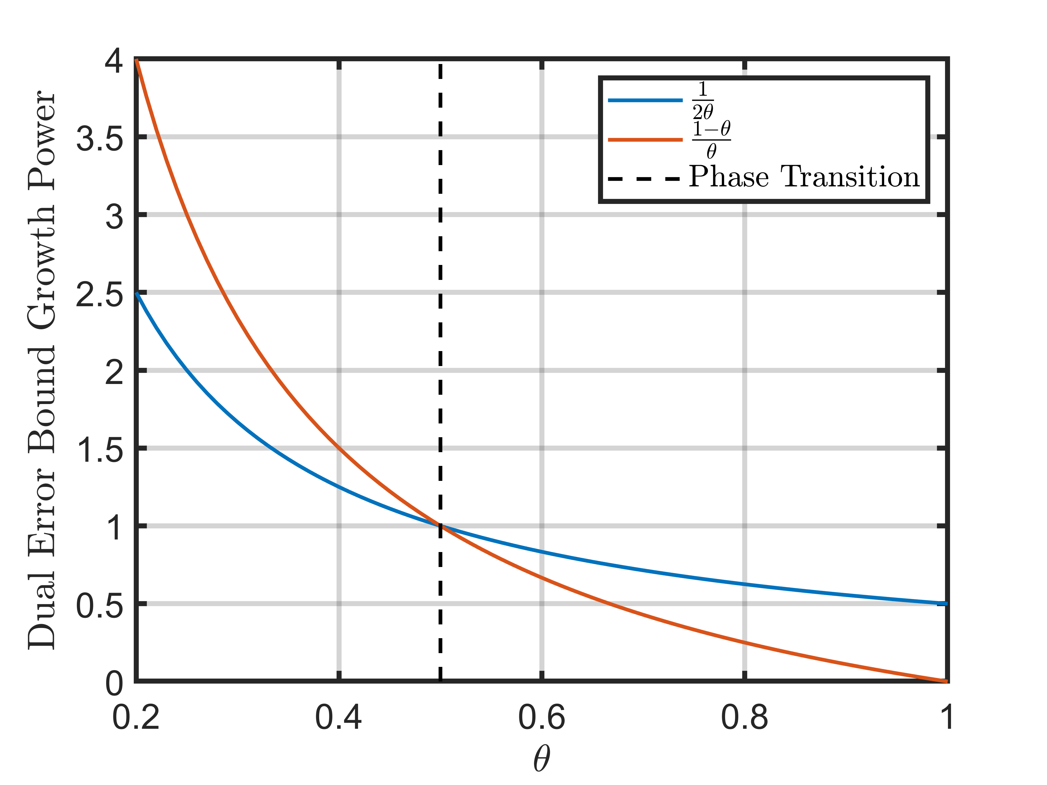
Figure 1: Comparison between the dual error bound (Proposition 3) and the pure dual error bound.

6 Verification of KŁ Property

As we have seen from the last section, the KŁ property (Assumption 2) is crucial to establishing the iteration complexity of our proposed smoothed PLDA. In this section, we show that Assumption 2 holds when the dual function is linear, i.e., problem (P) takes the form

$$\min_{x\in\mathcal{X}}\max_{y\in\mathcal{Y}}\left\{F(x,y)=y^{\top}G(x)\right\},$$ (6.1)

where $G:\mathbb{R}^{n}\rightarrow\mathbb{R}^{d}$ is a continuously differentiable map with a Lipschitz continuous Jacobian and $\mathcal{Y}$ (assumed to be nonempty) is a polytope defined by

$$\mathcal{Y}=\{y\in\mathbb{R}^{d}:a_{i}^{\top}y\leq b_{i},\ i\in[l]\},$$

with $l\in\mathbb{N}$ and $a_{i}\in\mathbb{R}^{d}$, $b_{i}\in\mathbb{R}$ for $i\in[l]$.

Theorem 2 (KŁ exponent of linear dual function).

Consider problem (6.1). Suppose there exists a $\delta>0$ such that for any $x\in\mathcal{X}$ and $y^{\star}(x)\in\operatorname*{argmax}_{y\in\mathcal{Y}}y^{\top}G(x)$, we have $\lambda_{i}(x)\geq\delta$ for all $i\in\mathcal{I}(x)$, where $\mathcal{I}(x)=\{i:a_{i}^{\top}y^{\star}(x)=b_{i}\}\subseteq[l]$ is the active index set and $\lambda_{i}(x)$ is the dual variable associated with the constraint $a_{i}^{\top}y-b_{i}\leq 0$ for $i\in[d]$. Then, Assumption 2 holds with $\theta=0$.

Proof.

By adopting the convention $0^{0}=0$, we see that Assumption 2 holds with $\theta=0$ for any $x\in\mathcal{X}$ and $y\in\mathcal{Y}$ satisfying $F(x,y)=\max_{y^{\prime}\in\mathcal{Y}}F(x,y^{\prime})$. Hence, our goal is to show that there exists a $\mu>0$ satisfying

$$\operatorname{dist}(0,-G(x)+\partial\iota_{\mathcal{Y}}(y))\geq\mu\quad\text{for any}\ x\in\mathcal{X},\ y\in\mathcal{Y}_{-}(x),$$

where

$$\mathcal{Y}_{-}(x)=\mathcal{Y}\setminus\mathcal{Y}^{\star}(x)\quad\mbox{and}\quad\mathcal{Y}^{\star}(x) \ =\left\{y\in\mathcal{Y}:\max_{y^{\prime}\in\mathcal{Y}}F(x,y^{\prime})\leq F(x,y)\right\}=\operatorname*{argmax}_{y^{\prime}\in\mathcal{Y}}F(x,y^{\prime}).$$

In view of the equivalence between the weak sharp minimum property and the KŁ property with exponent $\theta=0$ for convex functions (Bolte et al.,, 2017, Theorem 5), it suffices to show that

$$\mu\cdot\operatorname{dist}\left(y,\mathcal{Y}^{\star}(x)\right)\leq\max\limits_{y^{\prime}\in\mathcal{Y}}F(x,y^{\prime})-F(x,y)\quad\text{for any}\ x\in\mathcal{X},\ y\in\mathcal{Y}.$$

Towards that end, let $x\in\mathcal{X}$ be arbitrary and consider the following linear programming problem:

$$\begin{array}[]{cll}\max\limits_{y^{\prime}\in\mathbb{R}^{d}}&F(x,y^{\prime})\\ \operatorname{s.t.}&a_{i}^{\top}y^{\prime}-b_{i}\leq 0,\quad\forall i\in[l].\end{array}$$ (6.2)

For any $\bar{y}\in\mathcal{Y}^{\star}(x)$, using the KKT condition of (6.2), we can find $\lambda_{i}(x)\geq 0$ for $i\in[l]$ such that

$$\left\{\begin{array}[]{lr}-G(x)+\sum_{i=1}^{l}\lambda_{i}(x)a_{i}=0,\\ \lambda_{i}(x)\cdot(a_{i}^{\top}\bar{y}-b_{i})=0,\quad i\in[l].\end{array}\right.$$ (6.3)

Moreover, if we let $\mathcal{L}(x):=\left\{y^{\prime}\in\mathbb{R}^{d}:(\lambda_{i}(x)a_{i})^{\top}y^{\prime}=\lambda_{i}(x)b_{i},\ i\in[l]\right\}$, then $\mathcal{Y}\cap\mathcal{L}(x)=\mathcal{Y}^{\star}(x).$

Now, observe that as $x$ varies over $\mathcal{X}$, there are at most $2^{l}$ different sets of active constraints in problem (6.2). This, together with the complementarity condition in (6.3), implies that there are at most $2^{l}$ different polyhedra in the set $\{\mathcal{L}(x):x\in\mathcal{X}\}$. Thus, by the linear regularity property of polyhedral sets (Bauschke and Borwein,, 1996, Corollary 5.26), there exists an absolute constant $\gamma_{0}>0$ such that for all $y\in\mathcal{Y}$,

$$\operatorname{dist}(y,\mathcal{Y}^{\star}(x))=\operatorname{dist}(y,\mathcal{Y}\cap\mathcal{L}(x))\leq\gamma_{0}\cdot\operatorname{dist}(y,\mathcal{L}(x)).$$ (6.4)

Similarly, by Hoffman’s error bound (Hoffman,, 2003), there exists an absolute constant $\gamma_{1}>0$ such that for all $y\in\mathcal{Y}$,

$${\rm dist}(y,\mathcal{L}(x)) \ \leq\gamma_{1}\cdot\sum_{\lambda_{i}(x)>0}\left|a_{i}^{\top}y-b_{i}\right|=\gamma_{1}\cdot\sum_{\lambda_{i}(x)>0}\frac{1}{\lambda_{i}(x)}\left|\lambda_{i}(x)\cdot(a_{i}^{\top}y-b_{i})\right|.$$ (6.5)

Since $\lambda_{i}(x)\geq\delta$ if $\lambda_{i}(x)\neq 0$ by assumption, we get from (6.4) and (6.5) that

$${\rm dist}\left(y,\mathcal{Y}^{\star}(x)\right)\leq\frac{\gamma}{\delta}\cdot\sum_{i=1}^{l}|\lambda_{i}(x)\cdot(a_{i}^{\top}y-b_{i})|,$$ (6.6)

where $\gamma:=\gamma_{0}\gamma_{1}$. In addition, we have

$$\sum_{i=1}^{l}|\lambda_{i}(x)\cdot(a_{i}^{\top}y-b_{i})|=-\sum_{i=1}^{l}\lambda_{i}(x)\cdot(a_{i}^{\top}y-b_{i})$$ (6.7)

$$= \ -y^{\top}G(x)+\sum_{i=1}^{l}\lambda_{i}(x)\cdot a_{i}^{\top}\bar{y}=-F(x,y)+\max_{y^{\prime}\in\mathcal{Y}}F(x,y^{\prime}),$$

where the second and last equalities follow from (6.3). Putting (6.6) and (6.7) together yields

$$\mu\cdot{\rm dist}\left(y,\mathcal{Y}^{\star}(x)\right)\leq\max_{y^{\prime}\in\mathcal{Y}}F(x,y^{\prime})-F(x,y)$$

for all $y\in\mathcal{Y}$, where $\mu=\frac{\delta}{\gamma}$. The proof is then complete. ∎

Corollary 2 (Max-structured problem).

Consider problem (6.1), where $\mathcal{Y}=\{y\in\mathbb{R}^{d}:\sum_{i=1}^{d}y_{i}=1,\ y\geq 0\}$ is the standard simplex. Suppose there exists a $\delta>0$ such that for all $x\in\mathcal{X}$ and $j\in\mathcal{I}(x)$,

$$\max_{i\in[d]}\,G_{i}(x)\geq G_{j}(x)+\delta.$$ (6.8)

Then, Assumption 2 holds with $\theta=0$.

Proof.

Let $x\in\mathcal{X}$ and $y^{\star}(x)\in\operatorname*{argmax}_{y\in\mathcal{Y}}y^{\top}G(x)$ be arbitrary. Since $\mathcal{Y}$ is the standard simplex, the KKT condition (6.3) implies that

$$G(x)=(u(x)-\lambda_{1}(x),\ldots,u(x)-\lambda_{d}(x)),$$

where $\lambda_{i}(x)\geq 0$ (resp., $u(x)\in\mathbb{R}$) is the dual variable associated with the constraint $y_{i}\geq 0$ for $i\in[d]$ (resp., $\sum_{i=1}^{d}y_{i}=1$). If $y_{i}^{\star}(x)>0$ for some $i\in[d]$, then $\lambda_{i}(x)=0$, which implies that $\max_{i\in[d]}G_{i}(x)=u(x)$. On the other hand, condition (6.8) implies that for any $j\in[d]$ with $y_{j}^{\star}(x)=0$, we have

$$\lambda_{j}(x)=u(x)-(u(x)-\lambda_{j}(x))=\max_{i\in[d]}\,G_{i}(x)-G_{j}(x)\geq\delta.$$

Therefore, by applying Theorem 2, we conclude that problem (6.1) satisfies Assumption 2 with $\theta=0$. ∎

Remark 7.

(i) According to Remark 5(ii), the results in Theorem 2 and Corollary 2 remain valid under the weaker assumption that the KŁ property holds locally around any GS of problem (P), cf. Assumption 2. (ii) The work (Zhang et al.,, 2020) establishes a dual error bound for the max-structured problem under the assumptions that the primal function satisfies the gradient Lipschitz continuity condition and certain strict complementarity condition (see (Zhang et al.,, 2020, Assumption 3.5)) holds. It can be shown that the latter implies condition (6.8) in Corollary 2. However, it should be noted that the proof technique used in (Zhang et al.,, 2020) cannot be extended to the nonsmooth composite setting considered in this paper.

7 Quantitative Relationships among Different Stationarity Concepts

A fundamental question in the study of minimax optimization is how to define the concept of stationarity. One approach is to consider various natural optimality conditions of the minimax problem and extract from them the corresponding stationarity concepts. In the nonconvex-nonconcave setting, the different stationarity concepts obtained via this approach may not coincide, and their relationships are still not well understood. In this section, we aim to elucidate the relationships among several well-known stationarity concepts for problem (P). Interestingly, the dual error bound we developed in Corollary 1 plays an important role in obtaining our results.

To begin, let us consider the following exact stationarity concepts for problem (P):

Definition 2 (see, e.g., (Jin et al.,, 2020; Razaviyayn et al.,, 2020)).

The point $(x^{\star},y^{\star})\in\mathcal{X}\times\mathcal{Y}$ is called a

1. minimax point (MM) of problem (P) if

   $$F(x^{\star},y)\leq F(x^{\star},y^{\star})\leq\max_{y^{\prime}\in\mathcal{Y}}F(x,y^{\prime})\quad\text{for any }(x,y)\in\mathcal{X}\times\mathcal{Y};$$

2. game-stationary point (GS) of problem (P) if

   $$0\in\partial_{x}F(x^{\star},y^{\star})+\partial\iota_{\mathcal{X}}(x^{\star})\quad\text{and}\quad 0\in-\nabla_{y}F(x^{\star},y^{\star})+\partial\iota_{\mathcal{Y}}(y^{\star}).$$

Furthermore, the point $x^{\star}\in\mathcal{X}$ is called an

1. optimization-stationary point (OS) of problem (P) if

   $$0\in\partial(f+\iota_{\mathcal{X}})(x^{\star})=\partial\left(\max_{y\in\mathcal{Y}}F(\cdot,y)+\iota_{\mathcal{X}}\right)(x^{\star}).$$

The extreme value theorem guarantees the existence of an MM when $\mathcal{X}$ is compact, even if $F(\cdot,\cdot)$ is nonconvex-nonconcave. In addition, the weak convexity of $F(\cdot,y)$ and $-F(x,\cdot)$ for any $x\in\mathcal{X}$ and $y\in\mathcal{Y}$ ensures the existence of a GS (Pang and Razaviyayn,, 2016, Proposition 4.2). However, it is worth noting that finding a local MM (which may not even be an MM) of a constrained nonconvex-nonconcave optimization problem with a smooth objective is already hard (Daskalakis et al.,, 2021). Also, since most applications in machine learning, such as GANs and adversarial training, involve sequential games, the optimization-stationarity concept may be more attractive.

While the above definition of OS is standard, it only characterizes the primal variable $x$. As such, the concept of OS is not directly comparable to that of MM or GS. To circumvent this difficulty, we introduce the concept of an extended OS (eOS). Specifically, the point $(x^{\star},y^{\star})\in\mathcal{X}\times\mathcal{Y}$ is called an eOS of problem (P) if $x^{\star}$ is an OS and $F(x^{\star},y)\leq F(x^{\star},y^{\star})$ for any $y\in\mathcal{Y}$. From Definition 2, we can immediately conclude that every MM is an eOS. To gain some intuition on the possible relationships among the three types of stationarity points MM, GS, and eOS, it is instructive to consider the following example.

Figure 2: Possible relationships among the three types of stationarity points MM, GS, and eOS: (a) $F(x,y)=x^{3}-2xy-y^{2}$ with $\mathcal{X}\times\mathcal{Y}=[-1,1]\times[-1,1]$; (b) $F(x,y)=\sin(x)y$ with $\mathcal{X}\times\mathcal{Y}=[-\frac{\pi}{2},\frac{\pi}{2}]\times[-1,1]$; (c) $F(x,y)=xy$ with $\mathcal{X}\times\mathcal{Y}=\mathbb{R}\times[-1,1]$.

Example 1.

The following instances of problem (P) give rise to the relationships among MM, GS, and eOS shown in Figure 2.

1. If $F(x,y)=x^{3}-2xy-y^{2}$ and $\mathcal{X}\times\mathcal{Y}=[-1,1]\times[-1,1]$, then

   $$\mathrm{MM}=\left\{(-1,1),(0,0)\right\},\ \mathrm{GS}=\mathrm{eOS}=\left\{(-1,1),\left(-\frac{2}{3},\frac{2}{3}\right),(0,0)\right\}.$$

2. If $F(x,y)=\sin(x)y$ and $\mathcal{X}\times\mathcal{Y}=[-\frac{\pi}{2},\frac{\pi}{2}]\times[-1,1]$, then

   $$\mathrm{MM}=\left\{(0,[-1,1])\right\},\ \mathrm{GS}=\left\{\left(-\frac{\pi}{2},-1\right),(0,0),\left(\frac{\pi}{2},1\right)\right\},$$

   $$\mathrm{eOS}=\left\{\left(-\frac{\pi}{2},-1\right),(0,[-1,1]),\left(\frac{\pi}{2},1\right)\right\}.$$

3. If $F(x,y)=xy$ and $\mathcal{X}\times\mathcal{Y}=\mathbb{R}\times[-1,1]$, then

   $$\mathrm{GS}=\left\{(0,0)\right\},\ \mathrm{MM}=\mathrm{eOS}=\left\{(0,[-1,1])\right\}.$$

As we can see from Figure 2, the set of GS can fail to capture that of MM. Now, in view of the hardness of computing an MM, let us focus on expounding the relationship between the concepts of game stationarity and optimization stationarity. In fact, we shall address the more general problem of relating the approximate versions of these concepts as introduced in Definition 1.

To begin, let $x\in\mathcal{X}$ be arbitrary. Observe that since $f+\iota_{\mathcal{X}}$ is $L$-weakly convex on $\mathcal{X}$ (see Fact 1 in Appendix A) and $r>L$ by assumption, we have

$$\operatorname{dist}\left(0,\partial(f+\iota_{\mathcal{X}})\left(\operatorname{prox}_{\frac{1}{r}f+\iota_{\mathcal{X}}}(x)\right)\right)\leq r\left\|\operatorname{prox}_{\frac{1}{r}f+\iota_{\mathcal{X}}}(x)-x\right\|;$$

see, e.g., (Davis and Drusvyatskiy,, 2019, Section 2.2). It follows from Definition 1 that for problem (P), a $0$-OS is an OS. Similarly, since $F(\cdot,y)+\iota_{\mathcal{X}}(\cdot)$ is $L$-weakly convex on $\mathcal{X}$ for any $y\in\mathcal{Y}$, we have

$$\operatorname{dist}\left(0,\partial(F(\cdot,y)+\iota_{\mathcal{X}})\left(\operatorname{prox}_{\frac{1}{r}F(\cdot,y)+\iota_{\mathcal{X}}}(x)\right)\right) \leq r\left\|\operatorname{prox}_{\frac{1}{r}F(\cdot,y)+\iota_{\mathcal{X}}}(x)-x\right\|=\left\|\nabla_{z}d_{r}(y,x)\right\|,$$

where the last equality is due to Lemma 3 in Appendix A. It follows from Definition 1 that for problem (P), a $0$-GS is a GS. Based on the above, we may regard $\epsilon$-OS and $\epsilon$-GS as smoothed surrogates of OS and GS, respectively.

Remark 8.

When $F(x,\cdot)$ is concave for any $x\in\mathcal{X}$, each OS $x^{\star}$ has a corresponding GS whose $x$-coordinate is $x^{\star}$. To be more precise, if $x^{\star}$ is an OS, then we have $x_{r}^{\star}(x^{\star})=\operatorname{prox}_{\frac{1}{r}f+\iota_{\mathcal{X}}}(x^{\star})=x^{\star}$. Consequently, for any $y\in\mathcal{Y}$, we can bound the game-stationarity measure of $(x^{\star},y)$ as

$$\ \frac{1}{r}\|\nabla_{z}d_{r}(y,x^{\star})\|=\|x_{r}(y,x^{\star})-x^{\star}\|$$

$$\leq \ \|x_{r}(y,x^{\star})-x_{r}(y_{+}(x^{\star}),x^{\star})\|+\|x_{r}(y_{+}(x^{\star}),x^{\star})-x_{r}^{\star}(x^{\star})\|+\|\operatorname{prox}_{\frac{1}{r}f+\iota_{\mathcal{X}}}(x^{\star})-x^{\star}\|$$

$$\leq \ \sigma_{2}\|y-y_{+}(x^{\star})\|+\kappa^{\frac{1}{2}}\|y-y_{+}(x^{\star})\|^{\frac{1}{2}}$$

$$= \ \mathcal{O}\left({\rm dist}(0,-\nabla_{y}d_{r}(y,x^{\star})+\partial\iota_{\mathcal{Y}}(y))+\operatorname{dist}^{\frac{1}{2}}(0,-\nabla_{y}d_{r}(y,x^{\star})+\partial\iota_{\mathcal{Y}}(y))\right),$$

where the second inequality follows from Lemma 2, Lemma 8, and the fact that $\operatorname{prox}_{\frac{1}{r}f+\iota_{\mathcal{X}}}(x^{\star})=x^{\star}$, and the last equality is due to (Li and Pong,, 2018, Lemma 4.1) and Lemma 3 in Appendix A. Now, observe that

$$\max_{y\in\mathcal{Y}}d_{r}(y,x^{\star}) \ =\max_{y\in\mathcal{Y}}\min_{x\in\mathcal{X}}\left\{F(x,y)+\frac{r}{2}\|x-x^{\star}\|^{2}\right\}$$

$$\ =\min_{x\in\mathcal{X}}\max_{y\in\mathcal{Y}}\left\{F(x,y)+\frac{r}{2}\|x-x^{\star}\|^{2}\right\}=\max_{y\in\mathcal{Y}}F(x^{\star},y),$$

where the second equality is due to the convexity of $F_{r}(\cdot,y,x^{\star})$ for any $y\in\mathcal{Y}$ (recall that $r>L$ by assumption) and concavity of $F(x,\cdot)$ for any $x\in\mathcal{X}$, and the last equality is from $\operatorname{prox}_{\frac{1}{r}f+\iota_{\mathcal{X}}}(x^{\star})=x^{\star}$. Since an optimal solution $y^{\star}(x^{\star})$ of the above problem satisfies

$$0\in-\nabla_{y}d_{r}(y^{\star}(x^{\star}),x^{\star})+\partial\iota_{\mathcal{Y}}(y^{\star}(x^{\star}))=-\nabla_{y}F(x^{\star},y^{\star}(x^{\star}))+\partial\iota_{\mathcal{Y}}(y^{\star}(x^{\star}))$$

and thus also $\|\nabla_{z}d_{r}(y^{\star}(x^{\star}),x^{\star})\|=0$, we conclude that $(x^{\star},y^{\star}(x^{\star}))$ is a GS.

Now, let us state the main result in this section, which establishes a quantitative, algorithm-independent relationship between the $\epsilon$-game-stationarity and $\epsilon$-optimization-stationarity concepts for any $\epsilon\in[0,1)$. The key tool used is the alternative dual error bound (Corollary 1) presented in Section 5.3.

Theorem 3.

Suppose that $(x,y)\in\mathcal{X}\times\mathcal{Y}$ is an $\epsilon$-GS of problem (P) for some $\epsilon\in[0,1)$. Then, the point $x$ is

1. (KŁ exponent $\theta\in[0,1)$): an $\mathcal{O}(\epsilon^{\min\{1,\frac{1}{2\theta}\}})$-OS of problem (P);

2. (General concave): an $\mathcal{O}(\epsilon^{\frac{1}{2}})$-OS of problem (P).

Proof.

For case (a), we first compute

$$\|\operatorname{prox}_{\frac{1}{r}f+\iota_{\mathcal{X}}}(x)-x\|=\ \|x_{r}^{\star}(x)-x\|$$

$$\leq\ \|x_{r}^{\star}(x)-x_{r}(y_{+}(x),x)\|+\|x_{r}(y_{+}(x),x)-x_{r}(y,x)\|+\|x_{r}(y,x)-x\|$$

$$\leq\ \omega\|y-y_{+}(x)\|^{\gamma}+\sigma_{2}\|y-y_{+}(x)\|+\frac{1}{r}\|\nabla_{z}d_{r}(y,x)\|,$$ (7.1)

where the last inequality follows from Corollary 1, Lemma 2, and Lemma 3 with $\omega$ being equal to $\omega_{2}$ (resp., $\omega_{1}$) and $\gamma$ being equal to $\tfrac{1}{2\theta}$ (resp., $1$) when $\theta\in(0,1)$ (resp., $\theta=0$).

Next, we estimate $\|y-y_{+}(x)\|$ in terms of the game-stationarity measure of $(x,y)$. Let $y_{\#}(x):=\operatorname{proj}_{\mathcal{Y}}(y+\alpha\nabla_{y}F(x,y))$. By (Li and Pong,, 2018, Lemma 4.1), we have

$$\|y-y_{\#}(x)\|\leq{\rm dist}(0,-\nabla_{y}F(x,y)+\partial\iota_{\mathcal{Y}}(y)).$$

Moreover, as $\mathcal{Y}$ is a convex set, we have

$$\|y_{\#}(x)-y_{+}(x)\| =\|\operatorname{proj}_{\mathcal{Y}}\left(y+\alpha\nabla_{y}F(x,y)\right)-\operatorname{proj}_{\mathcal{Y}}\left(y+\alpha\nabla_{y}F(x_{r}(y,x),y)\right)\|$$

$$\leq\alpha\|\nabla_{y}F(x,y)-\nabla_{y}F(x_{r}(y,x),y)\|$$

$$\leq\alpha L\|x_{r}(y,x)-x\|,$$

where the first inequality holds due to the nonexpansiveness of $\operatorname{proj}_{\mathcal{Y}}$ and the second inequality is due to the $L$-Lipschitz continuity of $\nabla_{y}F(\cdot,y)$ on $\mathcal{X}$. Putting the above together yields

$$\|y-y_{+}(x)\| \leq\|y-y_{\#}(x)\|+\|y_{\#}(x)-y_{+}(x)\|$$

$$\leq{\rm dist}(0,-\nabla_{y}F(x,y)+\partial\iota_{\mathcal{Y}}(y))+\alpha L\|x_{r}(y,x)-x\|.$$ (7.2)

Since $(x,y)\in\mathcal{X}\times\mathcal{Y}$ is an $\epsilon$-GS, we have

$$\|\nabla_{z}d_{r}(y,x)\|\leq\epsilon\quad\text{and}\quad{\rm dist}(0,-\nabla_{y}F(x,y)+\partial\iota_{\mathcal{Y}}(y))\leq\epsilon.$$

It follows that the optimization-stationarity measure of $x$ can be bounded as

$$\|\operatorname{prox}_{\frac{1}{r}f+\iota_{\mathcal{X}}}(x)-x\|$$

$$\leq\ \omega\|y-y_{+}(x)\|^{\gamma}+\sigma_{2}\|y-y_{+}(x)\|+\frac{1}{r}\|\nabla_{z}d_{r}(y,x)\|$$

$$\leq\ \omega\left({\rm dist}(0,-\nabla_{y}F(x,y)+\partial\iota_{\mathcal{Y}}(y))+\frac{\alpha L}{r}\|\nabla_{z}d_{r}(y,x)\|\right)^{\gamma}$$

$$+\sigma_{2}\left({\rm dist}(0,-\nabla_{y}F(x,y)+\partial\iota_{\mathcal{Y}}(y))+\frac{\alpha L}{r}\|\nabla_{z}d_{r}(y,x)\|\right)+\frac{1}{r}\|\nabla_{z}d_{r}(y,x)\|$$

$$\leq\ \omega\left(1+\frac{\alpha L}{r}\right)^{\gamma}\epsilon^{\gamma}+\sigma_{2}\left(1+\frac{\alpha L}{r}\right)\epsilon+\frac{\epsilon}{r}=\mathcal{O}(\epsilon^{\min\{1,\frac{1}{2\theta}\}}),$$

where the first inequality follows from (7) and the second from (7.2). This implies that $x$ is an $\mathcal{O}(\epsilon^{\min\{1,\frac{1}{2\theta}\}})$-OS of problem (P).

Now, for case (b), we can apply Lemma 8 to derive the inequality (7) with $\omega$ and $\gamma$ being replaced by $\sqrt{\kappa}$ and $\tfrac{1}{2}$, respectively. The remainder of the proof follows the same argument as that for case (a). ∎

Remark 9.

Theorem 3 expands on the findings of Propositions 4.11 and 4.12 in (Lin et al., 2020b, ) by covering a broader range of scenarios. Specifically, it applies to settings where (i) $\mathcal{X}$ is not necessarily the entire space $\mathbb{R}^{n}$; (ii) the primal function is nonsmooth or lacks gradient Lipschitz continuity; (iii) the dual problem may not be concave and only satisfies the KŁ property with exponent $\theta$. Furthermore, our results apply to the problems studied in (Zhang et al.,, 2020; Yang et al.,, 2022).

8 Closing Remarks

In this paper, we proposed smoothed PLDA for solving a class of nonsmooth composite nonconvex-nonconcave problems. When the dual function is concave, we showed that our algorithm can find both an $\epsilon$-GS and an $\epsilon$-OS of the problem in $\mathcal{O}(\epsilon^{-4})$ iterations, which is a first step towards matching the complexity results for smooth minimax problems. Moreover, when the dual function possesses the KŁ property with exponent $\theta\in[0,1)$, we showed that our algorithm has an iteration complexity of $\mathcal{O}(\epsilon^{-2\max\{2\theta,1\}})$. As it turns out, this complexity is determined by the slower of the primal and dual updates in smoothed PLDA and reveals an interesting phase transition phenomenon: When $\theta\in[0,\frac{1}{2}]$, the primal update, which involves solving a strongly convex problem, dominates. As such, we cannot break the optimal iteration complexity of $\mathcal{O}(\epsilon^{-2})$. On the other hand, when $\theta\in(\frac{1}{2},1)$, the dual update dominates and explicitly depends on $\theta$, resulting in an iteration complexity of $\mathcal{O}(\epsilon^{-4\theta})$. The insights gained from our analysis suggest a new algorithm design principle—namely, primal-dual balancing—which holds promise for the design of more efficient algorithms in the context of minimax optimization.

Our work suggests several directions for further study. We mention some of them here.

1. Extend our algorithm and its analysis to the stochastic setting to benefit modern machine learning tasks.

2. Investigate the lower complexity bounds of first-order methods for nonconvex-KŁ problems and their dependence on the KŁ exponent $\theta$. We conjecture that our proposed smoothed PLDA already has the optimal complexity, at least in terms of the dependence on $\theta$.

3. Identify additional structured nonconvex-nonconcave problems that satisfy the KŁ property and characterize their KŁ exponents.

Appendix A Useful Technical Lemmas

To begin, we introduce the concept of weakly convex functions, which plays an important role in our subsequent analysis.

Definition 3 (Weak convexity).

A function $\ell:\mathbb{R}^{n}\rightarrow\mathbb{R}$ is said to be $\rho$-weakly convex on a set $\mathcal{X}\subseteq\mathbb{R}^{n}$ for some constant $\rho\geq 0$ if for any $x,y\in\mathcal{X}$ and $\tau\in[0,1]$, we have

$$\ell(\tau x+(1-\tau)y)\leq\tau\ell(x)+(1-\tau)\ell(y)+\frac{\rho\tau(1-\tau)}{2}\|x-y\|^{2}.$$

The above definition is equivalent to the convexity of the function $\ell(\cdot)+\tfrac{\rho}{2}\|\cdot\|^{2}$ on $\mathcal{X}$.

Definition 4 (Proximal mapping).

Let $\ell:\mathbb{R}^{n}\rightarrow\mathbb{R}\cup\{+\infty\}$ be a proper lower-semicontinuous function. The proximal mapping of $\ell$ with parameter $\mu>0$ at the point $x\in\mathbb{R}^{n}$ is defined by

$$\operatorname{prox}_{\mu\ell}(x)=\mathop{\operatorname*{argmin}}_{y\in\mathbb{R}^{n}}\left\{\ell(y)+\frac{1}{2\mu}\|y-x\|^{2}\right\}.$$

By our assumptions on problem (P) (recall that $L=L_{h}L_{c}$ and $r>L$) and (Drusvyatskiy and Paquette,, 2019, Lemma 3.2 and Lemma 4.2), we have the following useful results:

Fact 1.

The functions $F(\cdot,y)$ for any $y\in\mathcal{Y}$ and $f$ are $L$-weakly convex on $\mathcal{X}$.

Fact 2.

Let $y\in\mathbb{R}^{d}$ and $r>0$ be given. For all $x,\bar{x}\in\mathcal{X}$, we have

$$-\frac{r^{-1}+L}{2}\|x-\bar{x}\|^{2}\leq F(x,y)-F_{\bar{x},r}(x,y)\leq\frac{-r^{-1}+L}{2}\|x-\bar{x}\|^{2}.$$

Using Definition 3 and Fact 1, we can deduce that $F_{r}(\cdot,y,z)$ is $(r-L)$-strongly convex for any $y\in\mathcal{Y}$ and $z\in\mathbb{R}^{n}$.

Lemma 2 and Lemma 3 are also essential to our analysis. The proofs of these lemmas are similar to thoes of Lemma B.2 and Lemma B.3 in (Zhang et al.,, 2020), respectively. For completeness, we present the proofs here.

Lemma 2.

For any $y,y^{\prime}\in\mathcal{Y}$ and $z,z^{\prime}\in\mathbb{R}^{n}$, we have

$$\|x_{r}(y,z)-x_{r}(y,z^{\prime})\|\leq\sigma_{1}\|z-z^{\prime}\|,$$ (A.1)

$$\|x_{r}^{\star}(z)-x_{r}^{\star}(z^{\prime})\|\leq\sigma_{1}\|z-z^{\prime}\|,$$ (A.2)

$$\|x_{r}(y,z)-x_{r}(y^{\prime},z)\|\leq\sigma_{2}\|y-y^{\prime}\|,$$ (A.3)

where $\sigma_{1}:=\frac{r}{r-L}$ and $\sigma_{2}:=\frac{2r-L}{r-L}$.

Proof.

From the definition of $F_{r}$, we know that for any $x\in\mathcal{X}$, $y\in\mathcal{Y}$, and $z,z^{\prime}\in\mathbb{R}^{n}$,

$$F_{r}(x,y,z^{\prime})-F_{r}(x,y,z)=\frac{r}{2}(\|x-z^{\prime}\|^{2}-\|x-z\|^{2})=\frac{r}{2}(\|z^{\prime}\|^{2}-2(z^{\prime}-z)^{\top}x-\|z\|^{2}).$$ (A.4)

Fact 1 implies that $F(\cdot,y)$ is $L$-weakly convex for any $y\in\mathcal{Y}$. Therefore, for any $x\in\mathcal{X}$, $y\in\mathcal{Y}$, and $z\in\mathbb{R}^{n}$, we have

$$F_{r}(x,y,z)-F_{r}(x_{r}(y,z),y,z)\geq\frac{r-L}{2}\|x-x_{r}(y,z)\|^{2}.$$ (A.5)

Combining (A.4) and (A.5) yields

$$F_{r}(x_{r}(y,z),y,z^{\prime})-F_{r}(x_{r}(y,z^{\prime}),y,z^{\prime})$$

$$=\ F_{r}(x_{r}(y,z),y,z^{\prime})-F_{r}(x_{r}(y,z),y,z)+F_{r}(x_{r}(y,z),y,z)-F_{r}(x_{r}(y,z^{\prime}),y,z)\,$$

$$-(F_{r}(x_{r}(y,z^{\prime}),y,z^{\prime})-F_{r}(x_{r}(y,z^{\prime}),y,z))$$

$$\leq\ \frac{r}{2}(\|z^{\prime}\|^{2}-2(z^{\prime}-z)^{\top}x_{r}(y,z)-\|z\|^{2})-\frac{r-L}{2}\|x_{r}(y,z)-x_{r}(y,z^{\prime})\|^{2}\,$$

$$-\frac{r}{2}(\|z^{\prime}\|^{2}-2(z^{\prime}-z)^{\top}x_{r}(y,z^{\prime})-\|z\|^{2})$$

$$\leq\ r(z^{\prime}-z)^{\top}(x_{r}(y,z^{\prime})-x_{r}(y,z))-\frac{r-L}{2}\|x_{r}(y,z)-x_{r}(y,z^{\prime})\|^{2}.$$ (A.6)

On the other hand, (A.5) implies that

$$F_{r}(x_{r}(y,z),y,z^{\prime})-F_{r}(x_{r}(y,z^{\prime}),y,z^{\prime})\geq\frac{r-L}{2}\|x_{r}(y,z)-x_{r}(y,z^{\prime})\|^{2}.$$

Combining this inequality with (A), we get

$$(r-L)\|x_{r}(y,z)-x_{r}(y,z^{\prime})\|^{2}\leq r(z^{\prime}-z)^{\top}(x_{r}(y,z^{\prime})-x_{r}(y,z)).$$

Using the Cauchy-Schwarz inequality, we obtain

$$\|x_{r}(y,z)-x_{r}(y,z^{\prime})\|\leq\frac{r}{r-L}\|z-z^{\prime}\|.$$

Therefore, we conclude that (A.1) holds with $\sigma_{1}=\frac{r}{r-L}$. Since $f=\max_{y\in\mathcal{Y}}F(\cdot,y)$ is also $L$-weakly convex by Fact 1, we can prove that (A.2) holds by using a similar argument as above.

We now proceed to prove (A.3). Using (A.5), we have

$$F_{r}(x_{r}(y^{\prime},z),y,z)-F_{r}(x_{r}(y,z),y,z)\geq\frac{r-L}{2}\|x_{r}(y,z)-x_{r}(y^{\prime},z)\|^{2},$$ (A.7)

$$F_{r}(x_{r}(y,z),y^{\prime},z)-F_{r}(x_{r}(y^{\prime},z),y^{\prime},z)\geq\frac{r-L}{2}\|x_{r}(y,z)-x_{r}(y^{\prime},z)\|^{2}.$$ (A.8)

Moreover, by the $L$-Lipschitz continuity of $\nabla_{y}F_{r}(x,\cdot,z)$ for any $x\in\mathcal{X}$ and $z\in\mathbb{R}^{n}$, we have

$$F_{r}(x_{r}(y,z),y^{\prime},z)-F_{r}(x_{r}(y,z),y,z)\leq\langle\nabla_{y}F_{r}(x_{r}(y,z),y,z),y^{\prime}-y\rangle+\frac{L}{2}\|y-y^{\prime}\|^{2}$$ (A.9)

and

$$F_{r}(x_{r}(y^{\prime},z),y,z)-F_{r}(x_{r}(y^{\prime},z),y^{\prime},z)\leq\langle\nabla_{y}F_{r}(x_{r}(y^{\prime},z),y^{\prime},z),y-y^{\prime}\rangle+\frac{L}{2}\|y-y^{\prime}\|^{2}.$$ (A.10)

Incorporating (A.7)–(A.10), we obtain

$$(r-L)\|x_{r}(y,z)-x_{r}(y^{\prime},z)\|^{2}\leq\langle\nabla_{y}F_{r}(x_{r}(y,z),y,z)-\nabla_{y}F_{r}(x_{r}(y^{\prime},z),y^{\prime},z),y^{\prime}-y\rangle+L\|y-y^{\prime}\|^{2}.$$

Since $\nabla_{y}F_{r}(\cdot,\cdot,z)=\nabla_{y}F(\cdot,\cdot)$ is $L$-Lipschitz for any $z\in\mathbb{R}^{n}$, we have

$$\|\nabla_{y}F_{r}(x_{r}(y,z),y,z)-\nabla_{y}F_{r}(x_{r}(y^{\prime},z),y^{\prime},z)\|$$

$$\leq\ \|\nabla_{y}F_{r}(x_{r}(y,z),y,z)-\nabla_{y}F_{r}(x_{r}(y,z),y^{\prime},z)\|+\|\nabla_{y}F_{r}(x_{r}(y,z),y^{\prime},z)-\nabla_{y}F_{r}(x_{r}(y^{\prime},z),y^{\prime},z)\|$$

$$\leq\ L(\|y-y^{\prime}\|+\|x_{r}(y^{\prime},z)-x_{r}(y,z)\|).$$

It follows that

$$(r-L)\|x_{r}(y,z)-x_{r}(y^{\prime},z)\|^{2}\leq L\|x_{r}(y^{\prime},z)-x_{r}(y,z)\|\cdot\|y-y^{\prime}\|+2L\|y-y^{\prime}\|^{2}.$$

Let $\zeta:=\frac{\|x_{r}(y,z)-x_{r}(y^{\prime},z)\|}{\|y-y^{\prime}\|}$. Then, the above inequality gives

$$\zeta^{2} \ \leq\frac{L}{r-L}\zeta+\frac{2L}{(r-L)}\leq\frac{1}{2}\zeta^{2}+\frac{L^{2}}{2(r-L)^{2}}+\frac{2L}{(r-L)}$$

$$\ \leq\frac{1}{2}\zeta^{2}+\frac{L^{2}+4L(r-L)}{2(r-L)^{2}}\leq\frac{1}{2}\zeta^{2}+\frac{(L+2(r-L))^{2}}{2(r-L)^{2}},$$

where the second inequality holds because $ab\leq\frac{1}{2}(a^{2}+b^{2})$ for any $a,b\in\mathbb{R}$. Thus, we get

$$\|x_{r}(y,z)-x_{r}(y^{\prime},z)\|\leq\frac{2r-L}{r-L}\|y-y^{\prime}\|,$$

which shows that (A.3) holds with $\sigma_{2}=\frac{2r-L}{r-L}$. The proof is complete. ∎

Lemma 3.

The dual function $d_{r}$ is differentiable on $\mathcal{Y}\times\mathbb{R}^{n}$ with

$$\nabla_{y}d_{r}(y,z)=\nabla_{y}F(x_{r}(y,z),y),$$

$$\nabla_{z}d_{r}(y,z)=\nabla_{z}F_{r}(x_{r}(y,z),y,z)=r(z-x_{r}(y,z))$$

for any $y\in\mathcal{Y}$ and $z\in\mathbb{R}^{n}$. Moreover, for any $y\in\mathcal{Y}$ and $z\in\mathbb{R}^{n}$, the gradients $\nabla_{y}d_{r}(\cdot,z)$ and $\nabla_{z}d_{r}(y,\cdot)$ are Lipschitz continuous, i.e.,

$$\|\nabla_{y}d_{r}(y^{\prime},z)-\nabla_{y}d_{r}(y^{\prime\prime},z)\|\leq L_{d_{r}}\|y^{\prime}-y^{\prime\prime}\|\quad\text{for all}\ y^{\prime},y^{\prime\prime}\in\mathcal{Y},$$

$$\|\nabla_{z}d_{r}(y,z^{\prime})-\nabla_{z}d_{r}(y,z^{\prime\prime})\|\leq L_{d_{r}}^{\prime}\|z^{\prime}-z^{\prime\prime}\|\quad\text{for all}\ z^{\prime},z^{\prime\prime}\in\mathbb{R}^{n},$$

where $L_{d_{r}}:=(\sigma_{2}+1)L$ and $L_{d_{r}}^{\prime}:=(\sigma_{1}+1)r$.

Proof.

Since $F_{r}(\cdot,y,z)$ is strongly convex, $F_{r}(x,\cdot,z)$ is weakly concave, and $F_{r}(x,y,\cdot)$ is strongly convex for any $x\in\mathcal{X}$, $y\in\mathcal{Y}$, and $z\in\mathbb{R}^{n}$, the function

$$d_{r}(\cdot,\cdot)=\min_{x\in\mathcal{X}}F_{r}(x,\cdot,\cdot)$$

is differentiable on $\mathcal{Y}\times\mathbb{R}^{n}$ due to (Rockafellar and Wets,, 2009, Theorem 10.31). In particular, for any $y\in\mathcal{Y}$ and $z\in\mathbb{R}^{n}$, one has

$$\nabla_{y}d_{r}(y,z)=\nabla_{y}F_{r}(x_{r}(y,z),y,z)=\nabla_{y}F(x_{r}(y,z),y).$$

Using (Drusvyatskiy and Paquette,, 2019, Lemma 4.3), we have

$$\nabla_{z}d_{r}(y,z)=\nabla_{z}F_{r}(x_{r}(y,z),y,z)=r(z-\operatorname{prox}_{\frac{1}{r}F(\cdot,y)+\iota_{\mathcal{X}}}(z))=r(z-x_{r}(y,z)).$$

It follows that for any $y^{\prime},y^{\prime\prime}\in\mathcal{Y}$,

$$\|\nabla_{y}d_{r}(y^{\prime},z)-\nabla_{y}d_{r}(y^{\prime\prime},z)\|$$

$$=\ \|\nabla_{y}F_{r}(x_{r}(y^{\prime},z),y^{\prime},z)-\nabla_{y}F_{r}(x_{r}(y^{\prime\prime},z),y^{\prime\prime},z)\|$$

$$\leq\ \|\nabla_{y}F_{r}(x_{r}(y^{\prime},z),y^{\prime},z)-\nabla_{y}F_{r}(x_{r}(y^{\prime},z),y^{\prime\prime},z)\|+\|\nabla_{y}F_{r}(x_{r}(y^{\prime},z),y^{\prime\prime},z)-\nabla_{y}F_{r}(x_{r}(y^{\prime\prime},z),y^{\prime\prime},z)\|$$

$$\leq\ L\|y^{\prime}-y^{\prime\prime}\|+L\|x_{r}(y^{\prime},z)-x_{r}(y^{\prime\prime},z)\|$$

$$\leq\ L\|y^{\prime}-y^{\prime\prime}\|+L\sigma_{2}\|y^{\prime}-y^{\prime\prime}\|\leq L_{d_{r}}\|y^{\prime}-y^{\prime\prime}\|,$$

where the third inequality is due to (A.3). Moreover, we have

$$\|\nabla_{z}d_{r}(y,z^{\prime})-\nabla_{z}d_{r}(y,z^{\prime\prime})\|=\ r\|z^{\prime}-x_{r}(y,z^{\prime})-(z^{\prime\prime}-x_{r}(y,z^{\prime\prime}))\|$$

$$\leq\ r\|z^{\prime}-z^{\prime\prime}\|+r\|x_{r}(y,z^{\prime})-x_{r}(y,z^{\prime\prime})\|$$

$$\leq\ r\|z^{\prime}-z^{\prime\prime}\|+r\sigma_{1}\|z^{\prime}-z^{\prime\prime}\|\leq L_{d_{r}}^{\prime}\|z^{\prime}-z^{\prime\prime}\|,$$

where the second inequality is due to (A.1). The proof is complete. ∎

Lemma 4.

For any $k\geq 0$, we have

$$\|y^{k+1}-y_{+}^{k}(z^{k+1})\|\leq\eta\|x^{k}-x^{k+1}\|+\sigma_{1}\alpha L\|z^{k+1}-z^{k}\|,$$

where $\eta:=\alpha L\zeta$.

Proof.

We compute

$$\|y^{k+1}-y_{+}^{k}(z^{k+1})\|$$

$$= \|\operatorname{proj}_{\mathcal{Y}}(y^{k}+\alpha\nabla_{y}F(x^{k+1},y^{k}))-\operatorname{proj}_{\mathcal{Y}}(y^{k}+\alpha\nabla_{y}F(x_{r}(y^{k},z^{k+1}),y^{k}))\|$$

$$\leq \|y^{k}+\alpha\nabla_{y}F(x^{k+1},y^{k})-(y^{k}+\alpha\nabla_{y}F(x_{r}(y^{k},z^{k+1}),y^{k}))\|$$

$$\leq \alpha L(\|x^{k+1}-x_{r}(y^{k},z^{k})\|+\|x_{r}(y^{k},z^{k})-x_{r}(y^{k},z^{k+1})\|)$$

$$\leq \eta\|x^{k}-x^{k+1}\|+\sigma_{1}\alpha L\|z^{k+1}-z^{k}\|,$$

where the first inequality is due to the nonexpansiveness of the projection operator, the second is due to the $L$-Lipschitz continuity of $\nabla_{y}F(\cdot,\cdot)$, and the third follows from Proposition 2 and (A.1). The proof is complete. ∎

Appendix B Sufficient Decrease Property of Lyapunov Function

Lemma 5 (Primal descent).

For any $k\geq 0$, we have

$$F_{r}(x^{k},y^{k},z^{k})-F_{r}(x^{k+1},y^{k+1},z^{k+1})$$

$$\geq\ \frac{2\lambda^{-1}+r-L}{2}\|x^{k}-x^{k+1}\|^{2}+\langle\nabla_{y}F_{r}(x^{k+1},y^{k},z^{k}),y^{k}-y^{k+1}\rangle-\frac{L}{2}\|y^{k}-y^{k+1}\|^{2}$$

$$+\frac{(2-\beta)r}{2\beta}\|z^{k}-z^{k+1}\|^{2}.$$

Proof.

One can infer from the definition that $F_{x^{k},\lambda}(\cdot,y^{k})$ is $\lambda^{-1}$-strongly convex. Therefore, we have

$$F_{r}(x^{k},y^{k},z^{k}) =F(x^{k},y^{k})+\frac{r}{2}\|x^{k}-z^{k}\|^{2}=F_{x^{k},\lambda}(x^{k},y^{k})+\frac{r}{2}\|x^{k}-z^{k}\|^{2}$$

$$\geq F_{x^{k},\lambda}(x^{k+1},y^{k})+\frac{r}{2}\|x^{k+1}-z^{k}\|^{2}+\frac{\lambda^{-1}+r}{2}\|x^{k}-x^{k+1}\|^{2}.$$

Moreover, Fact 2 implies that

$$F_{x^{k},\lambda}(x^{k+1},y^{k})\geq F(x^{k+1},y^{k})+\frac{\lambda^{-1}-L}{2}\|x^{k+1}-x^{k}\|^{2}.$$

It follows that

$$F_{r}(x^{k},y^{k},z^{k}) \geq F(x^{k+1},y^{k})+\frac{r}{2}\|x^{k+1}-z^{k}\|^{2}+\frac{2\lambda^{-1}+r-L}{2}\|x^{k}-x^{k+1}\|^{2}$$

$$=F_{r}(x^{k+1},y^{k},z^{k})+\frac{2\lambda^{-1}+r-L}{2}\|x^{k}-x^{k+1}\|^{2}.$$ (B.1)

Next, as $\nabla_{y}F_{r}(x,\cdot,z)$ is $L$-Lipschitz continuous for any $x\in\mathcal{X}$ and $z\in\mathbb{R}^{n}$, we have

$$F_{r}(x^{k+1},y^{k},z^{k})-F_{r}(x^{k+1},y^{k+1},z^{k})\geq\langle\nabla_{y}F_{r}(x^{k+1},y^{k},z^{k}),y^{k}-y^{k+1}\rangle-\frac{L}{2}\|y^{k}-y^{k+1}\|^{2}.$$ (B.2)

At last, based on the update $z^{k+1}=z^{k}+\beta(x^{k+1}-z^{k})$, we get

$$F_{r}(x^{k+1},y^{k+1},z^{k})-F_{r}(x^{k+1},y^{k+1},z^{k+1})=\frac{(2-\beta)r}{2\beta}\|z^{k}-z^{k+1}\|^{2}.$$ (B.3)

By summing up (B), (B.2), and (B.3), we obtain the desired result. ∎

Lemma 6 (Dual ascent).

For any $k\geq 0$, we have

$$d_{r}(y^{k+1},z^{k+1})-d_{r}(y^{k},z^{k})$$

$$\geq \langle\nabla_{y}F_{r}(x_{r}(y^{k},z^{k}),y^{k},z^{k}),y^{k+1}-y^{k}\rangle-\frac{L_{d_{r}}}{2}\|y^{k}-y^{k+1}\|^{2}\,$$

$$+\frac{r}{2}\left\langle z^{k+1}-z^{k},z^{k+1}+z^{k}-2x_{r}(y^{k+1},z^{k+1})\right\rangle.$$

Proof.

Based on Lemma 3, $\nabla_{y}d_{r}(\cdot,z)$ is $L_{d_{r}}$-Lipschitz continuous for any $z\in\mathbb{R}^{n}$. Thus, we have

$$d_{r}(y^{k+1},z^{k})-d_{r}(y^{k},z^{k}) \geq\langle\nabla_{y}d_{r}(y^{k},z^{k}),y^{k+1}-y^{k}\rangle-\frac{L_{d_{r}}}{2}\|y^{k}-y^{k+1}\|^{2}$$

$$=\langle\nabla_{y}F_{r}(x_{r}(y^{k},z^{k}),y^{k},z^{k}),y^{k+1}-y^{k}\rangle-\frac{L_{d_{r}}}{2}\|y^{k}-y^{k+1}\|^{2}.$$

In addition, one has

$$d_{r}(y^{k+1},z^{k+1})-d_{r}(y^{k+1},z^{k})$$

$$=\ F_{r}(x_{r}(y^{k+1},z^{k+1}),y^{k+1},z^{k+1})-F_{r}(x_{r}(y^{k+1},z^{k}),y^{k+1},z^{k})$$

$$\geq\ F_{r}(x_{r}(y^{k+1},z^{k+1}),y^{k+1},z^{k+1})-F_{r}(x_{r}(y^{k+1},z^{k+1}),y^{k+1},z^{k})$$

$$=\ \frac{r}{2}\|x_{r}(y^{k+1},z^{k+1})-z^{k+1}\|^{2}-\frac{r}{2}\|x_{r}(y^{k+1},z^{k+1})-z^{k}\|^{2}$$

$$=\ \frac{r}{2}\left\langle z^{k+1}-z^{k},z^{k+1}+z^{k}-2x_{r}(y^{k+1},z^{k+1})\right\rangle.$$

Finally, by combining the above inequalities, the proof is complete. ∎

Lemma 7 (Proximal descent (smoothness)).

For any $k\geq 0$, we have

$$p_{r}(z^{k})-p_{r}(z^{k+1})\geq\frac{r}{2}\left\langle z^{k+1}-z^{k},2x_{r}(y(z^{k+1}),z^{k})-z^{k}-z^{k+1}\right\rangle,$$

where $y(z^{k+1})\in Y(z^{k+1})$.

Proof.

Recall that $p_{r}(z)=\max_{y\in\mathcal{Y}}d_{r}(y,z)$. Due to the definition of $y(z^{k+1})$, we have

$$p_{r}(z^{k+1})-p_{r}(z^{k}) \leq d_{r}(y(z^{k+1}),z^{k+1})-d_{r}(y(z^{k+1}),z^{k})$$

$$\leq F_{r}(x_{r}(y(z^{k+1}),z^{k}),y(z^{k+1}),z^{k+1})-F_{r}(x_{r}(y(z^{k+1}),z^{k}),y(z^{k+1}),z^{k})$$

$$=\frac{r}{2}\left\langle z^{k+1}-z^{k},z^{k+1}+z^{k}-2x_{r}(y(z^{k+1}),z^{k})\right\rangle,$$

where the second inequality follows from the fact that

$$F_{r}(x^{\prime},y,z)\geq\min_{x\in\mathcal{X}}F_{r}(x,y,z)=d_{r}(y,z)$$

for any $x^{\prime}\in\mathcal{X}$. The proof is complete. ∎

Proof of Proposition 1

From Lemmas 5, 6, and 7, we have

$$\Phi_{r}(x^{k},y^{k},z^{k})-\Phi_{r}(x^{k+1},y^{k+1},z^{k+1})$$

$$=\ F_{r}(x^{k},y^{k},z^{k})-F_{r}(x^{k+1},y^{k+1},z^{k+1})+2(d_{r}(y^{k+1},z^{k+1})-d_{r}(y^{k},z^{k}))+2(p_{r}(z^{k})-p_{r}(z^{k+1}))$$

$$\geq\ \frac{2\lambda^{-1}+r-L}{2}\|x^{k}-x^{k+1}\|^{2}+\frac{(2-\beta)r}{2\beta}\|z^{k}-z^{k+1}\|^{2}-\left(L_{d_{r}}+\frac{L}{2}\right)\|y^{k}-y^{k+1}\|^{2}\,$$

$$+\underbrace{\langle\nabla_{y}F_{r}(x^{k+1},y^{k},z^{k}),y^{k}-y^{k+1}\rangle+2\langle\nabla_{y}F_{r}(x_{r}(y^{k},z^{k}),y^{k},z^{k}),y^{k+1}-y^{k}\rangle}_{\text{\char 172}}\,$$

$$+\underbrace{2r\left\langle z^{k+1}-z^{k},x_{r}(y(z^{k+1}),z^{k})-x_{r}(y^{k+1},z^{k+1})\right\rangle}_{\text{\char 173}}.$$

First, we simplify the term ①. We know that

$$\text{\char 172}=\ \langle\nabla_{y}F_{r}(x^{k+1},y^{k},z^{k}),y^{k}-y^{k+1}\rangle+2\langle\nabla_{y}F_{r}(x_{r}(y^{k},z^{k}),y^{k},z^{k}),y^{k+1}-y^{k}\rangle$$

$$=\ \langle\nabla_{y}F_{r}(x^{k+1},y^{k},z^{k}),y^{k+1}-y^{k}\rangle+2\langle\nabla_{y}F_{r}(x_{r}(y^{k},z^{k}),y^{k},z^{k})-\nabla_{y}F_{r}(x^{k+1},y^{k},z^{k}),y^{k+1}-y^{k}\rangle.$$

For the first term, we have

$$\langle\nabla_{y}F_{r}(x^{k+1},y^{k},z^{k}),y^{k+1}-y^{k}\rangle =\langle\nabla_{y}F_{r}(x^{k+1},y^{k},z^{k})+\frac{1}{\alpha}(y^{k}-y^{k+1}),y^{k+1}-y^{k}\rangle+\frac{1}{\alpha}\|y^{k}-y^{k+1}\|^{2}$$

$$=\frac{1}{\alpha}\langle y^{k}+\alpha\nabla_{y}F_{r}(x^{k+1},y^{k},z^{k})-y^{k+1},y^{k+1}-y^{k}\rangle+\frac{1}{\alpha}\|y^{k}-y^{k+1}\|^{2}$$

$$\geq\frac{1}{\alpha}\|y^{k}-y^{k+1}\|^{2},$$

where the last inequality follows from the property of the projection operator and the dual update $y^{k+1}=\operatorname{proj}_{\mathcal{Y}}(y^{k}+\alpha\nabla_{y}F_{r}(x^{k+1},y^{k},z^{k}))$ (recall that $\nabla_{y}F_{r}(x,y,z)=\nabla_{y}F(x,y)$ for any $x\in\mathcal{X}$, $y\in\mathcal{Y}$, and $z\in\mathbb{R}^{n}$). For the remaining terms, we have

$$2\langle\nabla_{y}F_{r}(x_{r}(y^{k},z^{k}),y^{k},z^{k})-\nabla_{y}F_{r}(x^{k+1},y^{k},z^{k}),y^{k+1}-y^{k}\rangle$$

$$\geq -2\|\nabla_{y}F_{r}(x_{r}(y^{k},z^{k}),y^{k},z^{k})-\nabla_{y}F_{r}(x^{k+1},y^{k},z^{k})\|\cdot\|y^{k+1}-y^{k}\|$$

$$\geq -2L\|x^{k+1}-x_{r}(y^{k},z^{k})\|\cdot\|y^{k}-y^{k+1}\|$$

$$\geq -L\zeta^{2}\|y^{k}-y^{k+1}\|^{2}-L\zeta^{-2}\|x^{k+1}-x_{r}(y^{k},z^{k})\|^{2}$$

$$\geq -L\zeta^{2}\|y^{k}-y^{k+1}\|^{2}-L\|x^{k+1}-x^{k}\|^{2},$$

where the third inequality holds because $2|a||b|\leq\tau a^{2}+\tfrac{1}{\tau}b^{2}$ for any $a,b\in\mathbb{R}$ and $\tau>0$, and the last inequality follows from Proposition 2. Putting the above together, we obtain

$$\text{\char 172}\geq\left(\frac{1}{\alpha}-L\zeta^{2}\right)\|y^{k}-y^{k+1}\|^{2}-L\|x^{k+1}-x^{k}\|^{2}.$$ (B.4)

Next, we bound the term ② by

$$\text{\char 173}=\ 2r\left\langle z^{k+1}-z^{k},x_{r}(y(z^{k+1}),z^{k})-x_{r}(y^{k+1},z^{k+1})\right\rangle$$

$$=\ 2r\left\langle z^{k+1}-z^{k},x_{r}(y(z^{k+1}),z^{k})-x_{r}(y(z^{k+1}),z^{k+1})\right\rangle\,$$

$$+2r\left\langle z^{k+1}-z^{k},x_{r}(y(z^{k+1}),z^{k+1})-x_{r}(y^{k+1},z^{k+1})\right\rangle$$

$$\geq -2r\sigma_{1}\|z^{k+1}-z^{k}\|^{2}+2r\left\langle z^{k+1}-z^{k},x_{r}(y(z^{k+1}),z^{k+1})-x_{r}(y^{k+1},z^{k+1})\right\rangle$$

$$\geq -2r\sigma_{1}\|z^{k+1}-z^{k}\|^{2}-\frac{r}{7\beta}\|z^{k+1}-z^{k}\|^{2}-7r\beta\|x_{r}(y(z^{k+1}),z^{k+1})-x_{r}(y^{k+1},z^{k+1})\|^{2},$$ (B.5)

where the first inequality is due to (A.1) and the Cauchy-Schwarz inequality, and the second inequality again follows from the fact that $2|a||b|\leq\tau a^{2}+\tfrac{1}{\tau}b^{2}$ for any $a,b\in\mathbb{R}$ and $\tau>0$. Now, the inequalities (B.4) and (B) imply that

$$\Phi_{r}(x^{k},y^{k},z^{k})-\Phi_{r}(x^{k+1},y^{k+1},z^{k+1})$$

$$\geq\ \frac{2\lambda^{-1}+r-3L}{2}\|x^{k}-x^{k+1}\|^{2}+\left(\frac{1}{\alpha}-L_{d_{r}}-\frac{L}{2}-L\zeta^{2}\right)\|y^{k}-y^{k+1}\|^{2}\,$$

$$+\left(\frac{(2-\beta)r}{2\beta}-2r\sigma_{1}-\frac{r}{7\beta}\right)\|z^{k}-z^{k+1}\|^{2}-7r\beta\|x_{r}(y(z^{k+1}),z^{k+1})-x_{r}(y^{k+1},z^{k+1})\|^{2}.$$ (B.6)

By Lemma 4 and the fact that $\|u+v\|^{2}\leq 2(\|u\|^{2}+\|v\|^{2})$ for any $u,v\in\mathbb{R}^{d}$, we have

$$\|y^{k+1}-y^{k}\|^{2} =\|y^{k+1}-y_{+}^{k}(z^{k+1})+y_{+}^{k}(z^{k+1})-y^{k}\|^{2}$$

$$\geq\frac{1}{2}\|y^{k}-y_{+}^{k}(z^{k+1})\|^{2}-\|y^{k+1}-y_{+}^{k}(z^{k+1})\|^{2}$$

$$\geq\frac{1}{2}\|y^{k}-y_{+}^{k}(z^{k+1})\|^{2}-2\eta^{2}\|x^{k+1}-x^{k}\|^{2}-2\sigma_{1}^{2}\alpha^{2}L^{2}\|z^{k+1}-z^{k}\|^{2}.$$ (B.7)

Similarly, by Lemma 2 and Lemma 4, we have

$$\|x_{r}(y(z^{k+1}),z^{k+1})-x_{r}(y^{k+1},z^{k+1})\|^{2}$$

$$\leq\ 2\|x_{r}(y(z^{k+1}),z^{k+1})-x_{r}(y_{+}^{k}(z^{k+1}),z^{k+1})\|^{2}+2\|x_{r}(y_{+}^{k}(z^{k+1}),z^{k+1})-x_{r}(y^{k+1},z^{k+1})\|^{2}$$

$$\leq\ 2\|x_{r}(y(z^{k+1}),z^{k+1})-x_{r}(y_{+}^{k}(z^{k+1}),z^{k+1})\|^{2}+2\sigma_{2}^{2}\|y^{k+1}-y_{+}^{k}(z^{k+1})\|^{2}$$

$$\leq\ 2\|x_{r}(y(z^{k+1}),z^{k+1})-x_{r}(y_{+}^{k}(z^{k+1}),z^{k+1})\|^{2}+4\sigma_{2}^{2}\eta^{2}\|x^{k+1}-x^{k}\|^{2}+4\sigma_{2}^{2}\sigma_{1}^{2}\alpha^{2}L^{2}\|z^{k+1}-z^{k}\|^{2}.$$ (B.8)

Substituting (B) and (B) into (B) yields

$$\Phi_{r}(x^{k},y^{k},z^{k})-\Phi_{r}(x^{k+1},y^{k+1},z^{k+1})$$

$$\geq\ \left(\frac{2\lambda^{-1}+r-3L}{2}-28r\beta\sigma_{2}^{2}\eta^{2}\right)\|x^{k}-x^{k+1}\|^{2}\ +\left(\frac{1}{\alpha}-L_{d_{r}}-\frac{L}{2}-L\zeta^{2}\right)\cdot$$

$$\left(\frac{1}{2}\|y^{k}-y_{+}^{k}(z^{k+1})\|^{2}-2\eta^{2}\|x^{k+1}-x^{k}\|^{2}-2\sigma_{1}^{2}\alpha^{2}L^{2}\|z^{k+1}-z^{k}\|^{2}\right)\$$

$$+\left(\frac{(2-\beta)r}{2\beta}-2r\sigma_{1}-\frac{r}{7\beta}-28r\beta\sigma_{1}^{2}\sigma_{2}^{2}\alpha^{2}L^{2}\right)\|z^{k}-z^{k+1}\|^{2}$$

$$-14r\beta\|x_{r}(y(z^{k+1}),z^{k+1})-x_{r}(y_{+}^{k}(z^{k+1}),z^{k+1})\|^{2}.$$

Suppose that $r\geq 3L$, which implies that $L_{d_{r}}+\frac{L}{2}\leq 5L$. We observe the following:

• As $\alpha\leq\min\left\{\frac{1}{10L},\frac{1}{4L\zeta^{2}}\right\}$, we have $\frac{1}{\alpha}-L_{d_{r}}-\frac{L}{2}\geq\frac{1}{2\alpha}$ and $\frac{1}{2\alpha}-L\zeta^{2}\geq\frac{1}{4\alpha}.$

• As $\beta\leq\frac{1}{28}$ and $\sigma_{1}\leq\frac{3}{2}$, $\sigma_{2}\leq\frac{5}{2}$, we have

  $$\frac{(2-\beta)r}{2\beta}-2r\sigma_{1}-\frac{r}{7\beta}-28r\beta\sigma_{1}^{2}\sigma_{2}^{2}\alpha^{2}L^{2}-\frac{1}{2\alpha}\sigma_{1}^{2}\alpha^{2}L^{2}$$

  $$\geq\ \frac{6r}{7\beta}-\frac{7r}{2}-28r\beta\left(\frac{3}{2}\right)^{2}\left(\frac{5}{2}\right)^{2}\left(\frac{1}{10L}\right)^{2}L^{2}-\frac{r}{24}$$

  $$\geq\ \frac{r}{\beta}\left(\frac{6}{7}-4\beta-14\beta^{2}\right)\geq\frac{4r}{7\beta}.$$

• As $\lambda^{-1}\geq L$ and recalling that $\eta=\alpha L\zeta$, we have

  $$\alpha\leq\frac{1}{4L\zeta^{2}}=\frac{\lambda^{-1}}{4L^{2}\zeta^{2}}\frac{L}{\lambda^{-1}}\leq\frac{\lambda^{-1}}{4L^{2}\zeta^{2}}\quad\text{and}\quad\frac{\eta^{2}}{2\alpha}=\frac{\alpha L^{2}\zeta^{2}}{2}\leq\frac{1}{8\lambda}.$$

  Moreover, since $\beta\leq\tfrac{(r-L)^{2}}{14\alpha r(2r-L)^{2}}=\tfrac{1}{14\alpha r\sigma_{2}^{2}}$, we have

  $$28r\beta\sigma_{2}^{2}\eta^{2}\leq\frac{2\eta^{2}}{\alpha}\leq\frac{1}{2\lambda}\quad\text{and}\quad\frac{2\lambda^{-1}+r-3L}{2}-28r\beta\sigma_{2}^{2}\eta^{2}-\frac{\eta^{2}}{2\alpha}\geq\frac{3}{8\lambda}.$$

Putting everything together yields

$$\Phi_{r}(x^{k},y^{k},z^{k})-\Phi_{r}(x^{k+1},y^{k+1},z^{k+1})$$

$$\geq\ \frac{3}{8\lambda}\|x^{k}-x^{k+1}\|^{2}+\frac{1}{8\alpha}\|y^{k}-y_{+}^{k}(z^{k+1})\|^{2}+\frac{4r}{7\beta}\|z^{k}-z^{k+1}\|^{2}$$

$$-14r\beta\|x_{r}(y(z^{k+1}),z^{k+1})-x_{r}(y_{+}^{k}(z^{k+1}),z^{k+1})\|^{2}.$$

The proof is complete.

Appendix C Proof of Corollary 1

Proof.

The proof follows closely that of Proposition 3. Let $\psi:\mathbb{R}^{n}\times\mathbb{R}^{n}\rightarrow\mathbb{R}$ be the function defined by

$$\psi(x,z)=\max\limits_{y\in\mathcal{Y}}F_{r}(x,y,z)$$

and consider arbitrary $x\in\mathcal{X}$, $y\in\mathcal{Y}$, and $z\in\mathbb{R}^{n}$. Again, note that $\psi(\cdot,z)$ is $(r-L)$-strongly convex. This implies that

$$\psi(x,z)-\psi(x^{\star}_{r}(z),z)\geq\frac{r-L}{2}\|x-x^{\star}_{r}(z)\|^{2}.$$ (C.1)

Moreover, we have

$$\psi(x,z)-\psi(x_{r}^{\star}(z),z)$$

$$\leq\ \psi(x,z)-F_{r}(x_{r}(y_{+}(z),z),y_{+}(z),z)$$

$$=\ \max_{y^{\prime}\in\mathcal{Y}}F(x,y^{\prime})+\frac{r}{2}\|x-z\|^{2}-F_{r}(x_{r}(y_{+}(z),z),y_{+}(z),z)$$

$$=\, \max_{y^{\prime}\in\mathcal{Y}}F(x,y^{\prime})-F(x_{r}(y_{+}(z),z),y_{+}(z))+\frac{r}{2}\|x-z\|^{2}-\frac{r}{2}\|x_{r}(y_{+}(z),z)-z\|^{2},$$ (C.2)

where the inequality follows from

$$F_{r}(x_{r}(y_{+}(z),z),y_{+}(z),z)=\ \min_{x^{\prime}\in\mathcal{X}}\left\{F(x^{\prime},y_{+}(z))+\frac{r}{2}\|x^{\prime}-z\|^{2}\right\}$$

$$\leq\ \max_{y^{\prime}\in\mathcal{Y}}\min_{x^{\prime}\in\mathcal{X}}\left\{F(x^{\prime},y^{\prime})+\frac{r}{2}\|x^{\prime}-z\|^{2}\right\}$$

$$\leq\ \min_{x^{\prime}\in\mathcal{X}}\max_{y^{\prime}\in\mathcal{Y}}\left\{F(x^{\prime},y^{\prime})+\frac{r}{2}\|x^{\prime}-z\|^{2}\right\}=\psi(x_{r}^{\star}(z),z).$$

As (C.1) and (C) hold for any $x\in\mathcal{X}$, we obtain the intermediate relation

$$\frac{r-L}{2}\|x_{r}^{\star}(z)-x_{r}(y_{+}(z),z)\|^{2}\leq\max\limits_{y^{\prime}\in\mathcal{Y}}F(x_{r}(y_{+}(z),z),y^{\prime})-F(x_{r}(y_{+}(z),z),y_{+}(z))$$

by taking $x=x_{r}(y_{+}(z),z)$.

The remaining steps of the proof are the same as those of Proposition 3. For brevity, we omit them here. ∎

Appendix D Dual Error Bound for General Concave Case

The following lemma provides a dual error bound for the case where $F(x,\cdot)$ is concave for any $x\in\mathbb{R}^{n}$. Its proof is based on Lemma B.10 in (Zhang et al.,, 2020).

Lemma 8.

For any $y\in\mathcal{Y}$ and $z\in\mathbb{R}^{n}$, we have

$$\|x^{\star}_{r}(z)-x_{r}(y_{+}(z),z)\|^{2}\leq\kappa\|y-y_{+}(z)\|,$$

where $\kappa:=\frac{1+\alpha L\sigma_{2}+\alpha L}{\alpha(r-L)}\cdot{\rm diam}(\mathcal{Y})$.

Proof.

Let $y\in\mathcal{Y}$ and $z\in\mathbb{R}^{n}$ be arbitrary. Recall that $y(z)$ is an arbitrary vector in $Y(z)$. By the $(r-L)$-strong convexity of $F_{r}(\cdot,y,z)$, we have

$$F_{r}(x_{r}^{\star}(z),y_{+}(z),z)-F_{r}(x_{r}(y_{+}(z),z),y_{+}(z),z)\geq\frac{r-L}{2}\|x_{r}(y_{+}(z),z)-x^{\star}_{r}(z)\|^{2},$$

$$F_{r}(x_{r}(y_{+}(z),z),y(z),z)-F_{r}(x_{r}^{\star}(z),y(z),z)\geq\frac{r-L}{2}\|x_{r}(y_{+}(z),z)-x_{r}^{\star}(z)\|^{2}.$$

Moreover, since $(x_{r}^{\star}(z),y(z))$ is a saddle point of the convex-concave function $F_{r}(\cdot,\cdot,z)$ (Sion,, 1958), we have $F_{r}(x_{r}^{\star}(z),y(z),z)\geq F_{r}(x_{r}^{\star}(z),y_{+}(z),z)$, which implies that

$$F_{r}(x_{r}(y_{+}(z),z),y(z),z)-F_{r}(x_{r}(y_{+}(z),z),y_{+}(z),z)\geq(r-L)\|x_{r}(y_{+}(z),z)-x_{r}^{\star}(z)\|^{2}.$$ (D.1)

Note that $y_{+}(z)$ is the maximizer of

$$\max_{y^{\prime}\in\mathcal{Y}}\big{\langle}y+\alpha\nabla_{y}F_{r}(x_{r}(y,z),y,z)-y_{+}(z),y^{\prime}\big{\rangle}.$$

For simplicity, we define the function $\xi:\mathbb{R}^{d}\rightarrow\mathbb{R}$ by

$$\xi(\cdot):=\ \alpha F_{r}(x_{r}(y_{+}(z),z),\cdot,z)-\big{\langle}\alpha\nabla_{y}F_{r}(x_{r}(y_{+}(z),z),y_{+}(z),z),\cdot\big{\rangle}$$

$$-\big{\langle}y_{+}(z)-y-\alpha\nabla_{y}F_{r}(x_{r}(y,z),y,z),\cdot\big{\rangle}.$$

Then, we have

$$\max_{y^{\prime}\in\mathcal{Y}}\ \xi(y^{\prime})\leq\ \alpha F_{r}(x_{r}(y_{+}(z),z),y_{+}(z),z)-\big{\langle}\alpha\nabla_{y}F_{r}(x_{r}(y_{+}(z),z),y_{+}(z),z),y_{+}(z)\big{\rangle}\,$$

$$+\max_{y^{\prime}\in\mathcal{Y}}\big{\langle}y+\alpha\nabla_{y}F_{r}(x_{r}(y,z),y,z)-y_{+}(z),y^{\prime}\big{\rangle}$$

$$\leq\ \xi(y_{+}(z)),$$

where the first inequality holds because $F_{r}(x_{r}(y_{+}(z),z),\cdot,z)$ is concave. Therefore, we have $\xi(y(z))\leq\xi(y_{+}(z))$, which implies that

$$F_{r}(x_{r}(y_{+}(z),z),y(z),z)-F_{r}(x_{r}(y_{+}(z),z),y_{+}(z),z)$$

$$\leq \ \frac{1}{\alpha}\Big{\langle}y(z)-y_{+}(z),\alpha\nabla_{y}F_{r}(x_{r}(y_{+}(z),z),y_{+}(z),z)-\alpha\nabla_{y}F_{r}(x_{r}(y,z),y,z)\Big{\rangle}$$

$$\ +\frac{1}{\alpha}\Big{\langle}y(z)-y_{+}(z),y_{+}(z)-y\Big{\rangle}$$

$$\leq \ L\|y_{+}(z)-y(z)\|(\|x_{r}(y_{+}(z),z)-x_{r}(y,z)\|+\|y_{+}(z)-y\|)+\frac{1}{\alpha}\|y_{+}(z)-y(z)\|\cdot\|y-y_{+}(z)\|$$

$$\leq \ \left(\frac{1}{\alpha}+L\sigma_{2}+L\right)\|y_{+}(z)-y(z)\|\cdot\|y-y_{+}(z)\|.$$ (D.2)

Here, the second inequality is due to the $L$-Lipschitz continuity of $\nabla_{y}F_{r}(\cdot,\cdot,z)$ and the last inequality is from (A.3). Hence, by combining (D.1) and (D), we obtain

$$(r-L)\|x_{r}^{\star}(z)-x_{r}(y_{+}(z),z)\|^{2}\leq\left(\frac{1}{\alpha}+L\sigma_{2}+L\right){\rm diam}(\mathcal{Y})\cdot\|y-y_{+}(z)\|,$$

which proves the desired result. ∎

References

• Arjovsky et al., (2017) Arjovsky, M., Chintala, S., and Bottou, L. (2017). Wasserstein generative adversarial networks. In Proceedings of the 34th International Conference on Machine Learning (ICML 2017), pages 214–223. PMLR.
• Attouch et al., (2010) Attouch, H., Bolte, J., Redont, P., and Soubeyran, A. (2010). Proximal alternating minimization and projection methods for nonconvex problems: An approach based on the Kurdyka-Łojasiewicz inequality. Mathematics of Operations Research, 35(2):438–457.
• Attouch et al., (2013) Attouch, H., Bolte, J., and Svaiter, B. F. (2013). Convergence of descent methods for semi-algebraic and tame problems: Proximal algorithms, forward–backward splitting, and regularized Gauss–Seidel methods. Mathematical Programming, 137(1):91–129.
• Audibert and Catoni, (2011) Audibert, J.-Y. and Catoni, O. (2011). Robust linear least squares regression. The Annals of Statistics, 39(5):2766–2794.
• Barazandeh and Razaviyayn, (2020) Barazandeh, B. and Razaviyayn, M. (2020). Solving non-convex non-differentiable min-max games using proximal gradient method. In Proceedings of the 2020 IEEE International Conference on Acoustics, Speech, and Signal Processing, pages 3162–3166. IEEE.
• Bauschke and Borwein, (1996) Bauschke, H. H. and Borwein, J. M. (1996). On projection algorithms for solving convex feasibility problems. SIAM Review, 38(3):367–426.
• Bertsimas et al., (2011) Bertsimas, D., Brown, D. B., and Caramanis, C. (2011). Theory and applications of robust optimization. SIAM Review, 53(3):464–501.
• (8) Blanchet, J., Glynn, P. W., Yan, J., and Zhou, Z. (2019a). Multivariate distributionally robust convex regression under absolute error loss. In Advances in Neural Information Processing Systems 32.
• (9) Blanchet, J., Kang, Y., and Murthy, K. (2019b). Robust Wasserstein profile inference and applications to machine learning. Journal of Applied Probability, 56(3):830–857.
• Bolte et al., (2010) Bolte, J., Daniilidis, A., Ley, O., and Mazet, L. (2010). Characterizations of Łojasiewicz inequalities and applications. Transactions of the American Mathematical Society, 362(6):3319–3363.
• Bolte et al., (2017) Bolte, J., Nguyen, T. P., Peypouquet, J., and Suter, B. W. (2017). From error bounds to the complexity of first-order descent methods for convex functions. Mathematical Programming, 165(2):471–507.
• Boţ and Böhm, (2020) Boţ, R. I. and Böhm, A. (2020). Alternating proximal-gradient steps for (stochastic) nonconvex-concave minimax problems. arXiv preprint arXiv:2007.13605.
• Bubeck, (2015) Bubeck, S. (2015). Convex optimization: Algorithms and complexity. Foundations and Trends${}^{\text{\textregistered}}$ in Machine Learning, 8(3-4):231–357.
• Carmon et al., (2020) Carmon, Y., Duchi, J. C., Hinder, O., and Sidford, A. (2020). Lower bounds for finding stationary points I. Mathematical Programming, 184(1):71–120.
• Cartis et al., (2011) Cartis, C., Gould, N. I. M., and Toint, P. L. (2011). On the evaluation complexity of composite function minimization with applications to nonconvex nonlinear programming. SIAM Journal on Optimization, 21(4):1721–1739.
• Chen et al., (2021) Chen, Z., Zhou, Y., Xu, T., and Liang, Y. (2021). Proximal gradient descent-ascent: Variable convergence under KŁ geometry. In Proceedings of the 9th of International Conference on Learning Representations (ICLR 2021).
• Collins et al., (2020) Collins, L., Mokhtari, A., and Shakkottai, S. (2020). Task-robust model-agnostic meta-learning. In Advances in Neural Information Processing Systems 33.
• Cranko et al., (2021) Cranko, Z., Shi, Z., Zhang, X., Nock, R., and Kornblith, S. (2021). Generalised Lipschitz regularisation equals distributional robustness. In Proceedings of the 38th International Conference on Machine Learning (ICML 2021), pages 2178–2188. PMLR.
• Daskalakis et al., (2021) Daskalakis, C., Skoulakis, S., and Zampetakis, M. (2021). The complexity of constrained min-max optimization. In Proceedings of the 53rd Annual ACM SIGACT Symposium on Theory of Computing, pages 1466–1478.
• Davis and Drusvyatskiy, (2019) Davis, D. and Drusvyatskiy, D. (2019). Stochastic model-based minimization of weakly convex functions. SIAM Journal on Optimization, 29(1):207–239.
• Drusvyatskiy et al., (2021) Drusvyatskiy, D., Ioffe, A. D., and Lewis, A. S. (2021). Nonsmooth optimization using Taylor-like models: Error bounds, convergence, and termination criteria. Mathematical Programming, 185(1):357–383.
• Drusvyatskiy and Lewis, (2018) Drusvyatskiy, D. and Lewis, A. S. (2018). Error bounds, quadratic growth, and linear convergence of proximal methods. Mathematics of Operations Research, 43(3):919–948.
• Drusvyatskiy and Paquette, (2019) Drusvyatskiy, D. and Paquette, C. (2019). Efficiency of minimizing compositions of convex functions and smooth maps. Mathematical Programming, 178:503–558.
• Frankel et al., (2015) Frankel, P., Garrigos, G., and Peypouquet, J. (2015). Splitting methods with variable metric for Kurdyka-Łojasiewicz functions and general convergence rates. Journal of Optimization Theory and Applications, 165(3):874–900.
• Gao et al., (2022) Gao, R., Chen, X., and Kleywegt, A. J. (2022). Wasserstein distributionally robust optimization and variation regularization. Operations Research.
• Goodfellow et al., (2020) Goodfellow, I., Pouget-Abadie, J., Mirza, M., Xu, B., Warde-Farley, D., Ozair, S., Courville, A., and Bengio, Y. (2020). Generative adversarial networks. Communications of the ACM, 63(11):139–144.
• Hoffman, (2003) Hoffman, A. J. (2003). On approximate solutions of systems of linear inequalities. Journal of Research of the National Bureau of Standards, pages 174–176.
• Hu et al., (2023) Hu, Y., Li, C., Wang, J., Yang, X., and Zhu, L. (2023). Linearized proximal algorithms with adaptive stepsizes for convex composite optimization with applications. Applied Mathematics & Optimization, 87(3):52.
• Hu et al., (2016) Hu, Y., Li, C., and Yang, X. (2016). On convergence rates of linearized proximal algorithms for convex composite optimization with applications. SIAM Journal on Optimization, 26(2):1207–1235.
• Hu and Hong, (2013) Hu, Z. and Hong, L. J. (2013). Kullback-Leibler divergence constrained distributionally robust optimization. Available at Optimization Online, 1(2):9.
• Huang et al., (2021) Huang, F., Wu, X., and Huang, H. (2021). Efficient mirror descent ascent methods for nonsmooth minimax problems. In Advances in Neural Information Processing Systems 34.
• Jin et al., (2020) Jin, C., Netrapalli, P., and Jordan, M. (2020). What is local optimality in nonconvex-nonconcave minimax optimization? In Proceedings of the 37th of International Conference on Machine Learning (ICML 2020), pages 4880–4889. PMLR.
• Levy et al., (2020) Levy, D., Carmon, Y., Duchi, J. C., and Sidford, A. (2020). Large-scale methods for distributionally robust optimization. In Advances in Neural Information Processing Systems 33.
• Lewis and Wright, (2016) Lewis, A. S. and Wright, S. J. (2016). A proximal method for composite minimization. Mathematical Programming, 158:501–546.
• Li and Pong, (2018) Li, G. and Pong, T. K. (2018). Calculus of the exponent of Kurdyka-Łojasiewicz inequality and its applications to linear convergence of first-order methods. Foundations of Computational Mathematics, 18(5):1199–1232.
• Li et al., (2021) Li, H., Tian, Y., Zhang, J., and Jadbabaie, A. (2021). Complexity lower bounds for nonconvex-strongly-concave min-max optimization. In Advances in Neural Information Processing Systems 34.
• Li et al., (2020) Li, J., So, A. M.-C., and Ma, W.-K. (2020). Understanding notions of stationarity in nonsmooth optimization: A guided tour of various constructions of subdifferential for nonsmooth functions. IEEE Signal Processing Magazine, 37(5):18–31.
• (38) Lin, T., Jin, C., and Jordan, M. (2020a). Near-optimal algorithms for minimax optimization. In Proceedings of the 33rd Annual Conference on Learning Theory (COLT 2020), pages 2738–2779. PMLR.
• (39) Lin, T., Jin, C., and Jordan, M. (2020b). On gradient descent ascent for nonconvex-concave minimax problems. In Proceedings of the 37th International Conference on Machine Learning (ICML 2020), pages 6083–6093. PMLR.
• Lin et al., (2022) Lin, T., Jin, C., and Jordan, M. (2022). A nonasymptotic analysis of gradient descent ascent for nonconvex-concave minimax problems. Available at SSRN.
• Lu et al., (2020) Lu, S., Tsaknakis, I., Hong, M., and Chen, Y. (2020). Hybrid block successive approximation for one-sided non-convex min-max problems: Algorithms and applications. IEEE Transactions on Signal Processing, 68:3676–3691.
• Luo and Tseng, (1993) Luo, Z.-Q. and Tseng, P. (1993). Error bounds and convergence analysis of feasible descent methods: A general approach. Annals of Operations Research, 46(1):157–178.
• Madry et al., (2018) Madry, A., Makelov, A., Schmidt, L., Tsipras, D., and Vladu, A. (2018). Towards deep learning models resistant to adversarial attacks. In International Conference on Learning Representations.
• Mohri et al., (2019) Mohri, M., Sivek, G., and Suresh, A. T. (2019). Agnostic federated learning. In Proceedings of the 36th International Conference on Machine Learning (ICML 2019), pages 4615–4625. PMLR.
• Namkoong and Duchi, (2016) Namkoong, H. and Duchi, J. C. (2016). Stochastic gradient methods for distributionally robust optimization with $f$-divergences. In Advances in Neural Information Processing Systems 29.
• Nesterov, (2007) Nesterov, Y. (2007). Modified Gauss-Newton scheme with worst case guarantees for global performance. Optimization Methods and Software, 22(3):469–483.
• Nouiehed et al., (2019) Nouiehed, M., Sanjabi, M., Huang, T., Lee, J. D., and Razaviyayn, M. (2019). Solving a class of non-convex min-max games using iterative first order methods. In Advances in Neural Information Processing Systems 32.
• Ostrovskii et al., (2021) Ostrovskii, D. M., Lowy, A., and Razaviyayn, M. (2021). Efficient search of first-order Nash equilibria in nonconvex-concave smooth min-max problems. SIAM Journal on Optimization, 31(4):2508–2538.
• Pang and Razaviyayn, (2016) Pang, J.-S. and Razaviyayn, M. (2016). A unified distributed algorithm for non-cooperative games. In Cui, S., Hero, III, A. O., Luo, Z.-Q., and Moura, J. M., editors, Big Data over Networks, chapter 4. Cambridge University Press.
• Polyak, (1963) Polyak, B. T. (1963). Gradient methods for minimizing functionals. Zhurnal Vychislitel’noi Matematiki i Matematicheskoi Fiziki, 3(4):643–653.
• Rafique et al., (2022) Rafique, H., Liu, M., Lin, Q., and Yang, T. (2022). Weakly-convex–concave min–max optimization: Provable algorithms and applications in machine learning. Optimization Methods and Software, 37(3):1087–1121.
• Rahimian and Mehrotra, (2022) Rahimian, H. and Mehrotra, S. (2022). Frameworks and Results in Distributionally Robust Optimization. Open Journal of Mathematical Optimization.
• Razaviyayn et al., (2020) Razaviyayn, M., Huang, T., Lu, S., Nouiehed, M., Sanjabi, M., and Hong, M. (2020). Nonconvex min-max optimization: Applications, challenges, and recent theoretical advances. IEEE Signal Processing Magazine, 37(5):55–66.
• Rockafellar and Uryasev, (2000) Rockafellar, R. T. and Uryasev, S. (2000). Optimization of conditional value-at-risk. Journal of Risk, 2:21–42.
• Rockafellar and Wets, (2009) Rockafellar, R. T. and Wets, R. J.-B. (2009). Variational Analysis, volume 317. Springer Science & Business Media.
• Shafieezadeh-Abadeh et al., (2019) Shafieezadeh-Abadeh, S., Kuhn, D., and Esfahani, P. M. (2019). Regularization via mass transportation. Journal of Machine Learning Research, 20(103):1–68.
• Shalev-Shwartz and Wexler, (2016) Shalev-Shwartz, S. and Wexler, Y. (2016). Minimizing the maximal loss: How and why. In Proceedings of the 33rd International Conference on Machine Learning (ICML 2016), pages 793–801. PMLR.
• Sinha et al., (2018) Sinha, A., Namkoong, H., and Duchi, J. (2018). Certifying some distributional robustness with principled adversarial training. In Proceedings of the 6th International Conference on Learning Representations (ICLR 2018).
• Sion, (1958) Sion, M. (1958). On general minimax theorems. Pacific Journal of Mathematics, 8(1):171–176.
• Thekumparampil et al., (2019) Thekumparampil, K. K., Jain, P., Netrapalli, P., and Oh, S. (2019). Efficient algorithms for smooth minimax optimization. In Advances in Neural Information Processing Systems 32.
• Xu et al., (2023) Xu, Z., Zhang, H., Xu, Y., and Lan, G. (2023). A unified single-loop alternating gradient projection algorithm for nonconvex–concave and convex–nonconcave minimax problems. Mathematical Programming, pages 1–72.
• Yang et al., (2022) Yang, J., Orvieto, A., Lucchi, A., and He, N. (2022). Faster single-loop algorithms for minimax optimization without strong concavity. In Proceedings of the 25th International Conference on Artificial Intelligence and Statistics (AISTATS 2022), pages 5485–5517. PMLR.
• Yang et al., (2020) Yang, J., Zhang, S., Kiyavash, N., and He, N. (2020). A catalyst framework for minimax optimization. In Advances in Neural Information Processing Systems 33.
• Zhang and Luo, (2020) Zhang, J. and Luo, Z.-Q. (2020). A proximal alternating direction method of multiplier for linearly constrained nonconvex minimization. SIAM Journal on Optimization, 30(3):2272–2302.
• Zhang et al., (2020) Zhang, J., Xiao, P., Sun, R., and Luo, Z. (2020). A single-loop smoothed gradient descent-ascent algorithm for nonconvex-concave min-max problems. In Advances in Neural Information Processing Systems 33.
• Zhang and Zhou, (2018) Zhang, L. and Zhou, Z.-H. (2018). $\ell_{1}$-regression with heavy-tailed distributions. In Advances in Neural Information Processing Systems 31.
• Zhang et al., (2021) Zhang, S., Yang, J., Guzmán, C., Kiyavash, N., and He, N. (2021). The complexity of nonconvex-strongly-concave minimax optimization. In Proceedings of the 37th Conference on Uncertainty in Artificial Intelligence (UAI 2021), pages 482–492. PMLR.