Enhancing the Inductive Biases of Graph Neural ODE for Modeling Dynamical Systems

Abstract

Neural networks with physics-based inductive biases such as Lagrangian neural networks (Lnn), and Hamiltonian neural networks (Hnn) learn the dynamics of physical systems by encoding strong inductive biases. Alternatively, Neural ODEs with appropriate inductive biases have also been shown to give similar performances. However, these models, when applied to particle based systems, are transductive in nature and hence, do not generalize to large system sizes. In this paper, we present a graph-based neural ODE, Gnode, to learn the time evolution of dynamical systems. Further, we carefully analyse the role of different inductive biases on the performance of Gnode. We show that, similar to Lnn and Hnn, encoding the constraints explicitly can significantly improve the training efficiency and performance of Gnode significantly. Our experiments also assess the value of additional inductive biases, such as Newton’s third law, on the final performance of the model. We demonstrate that inducing these biases can enhance the performance of model by orders of magnitude in terms of both energy violation and rollout error. Interestingly, we observe that the Gnode trained with the most effective inductive biases, namely MCGnode, outperforms the graph versions of Lnn and Hnn, namely, Lagrangian graph networks (Lgn) and Hamiltonian graph networks (Hgn) in terms of energy violation error by $\sim$4 orders of magnitude for a pendulum system, and $\sim$2 orders of magnitude for spring systems. These results suggest that competitive performances with energy conserving neural networks can be obtained for Node-based systems by inducing appropriate inductive biases.

1 Introduction and related works

Learning the dynamics of physical systems is a challenging problem that has relevance in several areas of science and engineering such as astronomy (motion of planetary systems), biology (movement of cells), physics (molecular dynamics), and engineering (mechanics, robotics)[1, 2]. The dynamics of a system is typically expressed as a differential equation, solutions of which may require the knowledge of abstract quantities such as force, energy, and drag[1, 3, 4]. From an experimental perspective, the real observable for a physical system is its trajectory represented by the position and velocities of the constituent particles. Thus, learning the abstract quantities required to solve the equation, directly from the trajectory, can extremely simplify the problem of learning the dynamics [5].

Infusing physical laws as prior has been shown to improve the learning in terms of additional properties such as energy conservation, and symplectic nature [6, 7, 8]. To this extent, three broad approaches have been proposed, namely, Lagrangian neural networks (Lnn) [9, 5, 7], Hamiltonian neural networks (Hnn) [10, 11, 3, 12], and neural ODE (Node) [13, 14]. The learning efficiency of Lnns and Hnns is shown to enhance significantly by employing explicit constraints [5]. In addition, it has been shown that the superior performance of Hnns and Lnns is mainly due to their second order bias, and not due to their symplectic or energy conserving bias [14]. More specifically, an Hnn with separable potential ($V(q)$) and kinetic ($T(q,\dot{q})$) energies is equivalent to a second order Node of the form $\ddot{q}=\hat{F}(q,\dot{q})$. Thus, a Node with a second order bias can give similar performances to that of a Hnn [14].

An important limitation pervading these models is their transductive nature; they need to be trained on each system separately before simulating their dynamics. For instance, a Node trained on $5$-pendulum can work only for $5$-pendulum. This approach is referred to as transductive. In contrast, an inductive model, such as Gnode, when trained on $5$-pendulum "learns" the underlying function governing the dynamics at an node and edge level. Hence, a Gnode, once trained, can perform inference on any system size that are significantly smaller or larger than the ground truth as we demonstrate later in § 4. This inductive ability is enabled through Graph neural networks [15] due to their inherent topology-aware setting, which allows the learned system to naturally generalize. Although the idea of graph-based modeling have been suggested for physical systems [16, 11], the inductive biases induced due to different graph structures and their consequences on the dynamics remain poorly explored. Here, we carefully examine different inductive biases that can be encoded in a Node to model physical systems as follows.

1. Topology-aware modeling, where the physical system is modeled using a graph-based Node (Gnode).

2. Decoupling the dynamics and constraints, where the equation of motion of the Gnode is decoupled into the individual terms such as forces, Coriolis-like term and explicit constraints.

3. Decoupling the internal and body forces, where the internal forces due to the interaction among particles are decoupled from the forces due to external fields.

4. Newton’s third law, where the forces of interacting particles are enforced to be equal and opposite. We theoretically prove that this inductive bias enforces the conservation of linear momentum, in the absence of an external field, for the predicted trajectory exactly.

We analyze the role of these biases on $n$-pendulum and spring systems. Interestingly, depending on the nature of the system, we show that some these biases can either significantly improve the performance or have marginal effects. We also show that the final model with the appropriate inductive biases significantly outperform the simple version of Gnode with no additional inductive biases and even the graph versions of Lnn and Hnn.

2 Background on dynamical systems

A dynamical system can be defined by ordinary differential equations (ODEs) of the form, $\ddot{q}=F(q,\dot{q},t)$, where $F$ represents the dynamics of the system. Thus, the time evolution of the system can be obtained by integrating this equation of motion. In Lagrangian mechanics, the dynamics of a system is derived based on the Lagrangian of the system, which is defined as [2]:

$$L(q,\dot{q},t)=T(q,\dot{q})-V(q)$$ (1)

Once the Lagrangian of the system is computed, the dynamics can be obtained using the Euler-Lagrange (EL) equation as $\frac{d}{dt}\left(\nabla_{\dot{q}}L\right)=\nabla_{q}L$. Note that the EL equation is equivalent to the D’Alembert’s principle written in terms of the force as $\sum_{i=1}^{n}(N_{i}-m_{i}\ddot{q}_{i})\cdot\delta q_{i}=0$, where $\delta q_{i}$ represents a virtual displacement consistent with the constraints of the system. Thus, an alternative to the EL equation can be written in terms of the forces and other components as [1, 17]

$$M(q)\ddot{q}+C(q,\dot{q})\dot{q}+N(q)+\Upsilon(\dot{q})+A^{T}\lambda=\Pi$$ (2)

where $M(q)$ represents the mass matrix, $C(q,\dot{q})$ the Coriolis-like forces, $N(q)$ the conservative forces, $\Upsilon(\dot{q})$ represents the non-conservative forces such as drag or friction, and $\Pi$ represents any external forces. The constraints of the system are given by $A(q)\dot{q}=0$, where $A(q)\in\mathbb{R}^{k×D}$ represents $k$ constraints. Thus, $A$ represents the non-normalized basis of constraint forces given by $A=\nabla_{q}(\phi)$, where $\phi$ is the matrix corresponding to the constraints of the system and $\lambda$ is the Lagrange multiplier corresponding to the relative magnitude of the constraint forces. Note that $M,C,$ and $N$ are directly derivable from the Lagrangian of the system $L$ as $M=\nabla_{\dot{q}\dot{q}}L,C=\nabla_{q\dot{q}}L,$ and $N=\nabla_{q}L$. Thus, decoupling the dynamic equation simplifies the representation of the dynamics $F$ with enhanced interpretability. To learn the dynamics, Eq. 2 can be represented as

$$\ddot{q}=M^{-1}\left(\Pi-C\dot{q}-N-\Upsilon-A^{T}\lambda\right)$$ (3)

To solve for $\lambda$, the constraint equation can be differentiated with respect to time to obtain $A\ddot{q}+\dot{A}\dot{q}=0$. Substituting for $\ddot{q}$ from Eq. 3 and solving for $\lambda$, we get

$$\lambda=(AM^{-1}A^{T})^{-1}(AM^{-1}(\Pi-C\dot{q}-N-\Upsilon)+\dot{A}\dot{q})$$ (4)

Accordingly, $\ddot{q}$ can be obtained as

$$\ddot{q}=M^{-1}\left(\Pi-C\dot{q}-N-\Upsilon-A^{T}(AM^{-1}A^{T})^{-1}\left(AM^{-1}(\Pi-C\dot{q}-N-\Upsilon)+\dot{A}\dot{q}\right)\right)$$ (5)

3 Inductive biases for neural ODE

To learn the dynamical systems, Nodes parameterize the dynamics $F(q_{t},\dot{q}_{t})$ using a neural network and learn the approximate function $\hat{F}(q_{t},\dot{q}_{t})$ by minimizing the loss between the predicted and actual trajectories, that is, $\mathcal{L}=||q_{t+1}-\hat{q}_{t+1}||$. Thus, a Node essentially learns a cumulative $\hat{F}$, that consists of the contribution of all the terms contributing the dynamics. In contrast, in an Lnn, the learned $L$ is used in the EL equation to obtain the dynamics. Similarly, in Lnn with explicit constraints, the learned Lagrangian is used to obtain the individual terms in the Eq. 5 by differentiating the Lnn, which is then substituted to obtain the acceleration. However, this approach is transductive in nature. To overcome this challenge, we present a graph-based version of the Node namely, Gnode, which models the physical system as a graph. We show, that Gnode can generalize to arbitrary system size after learning the dynamics $\hat{F}$.

3.1 Graph neural ODE (Gnode) for physical systems

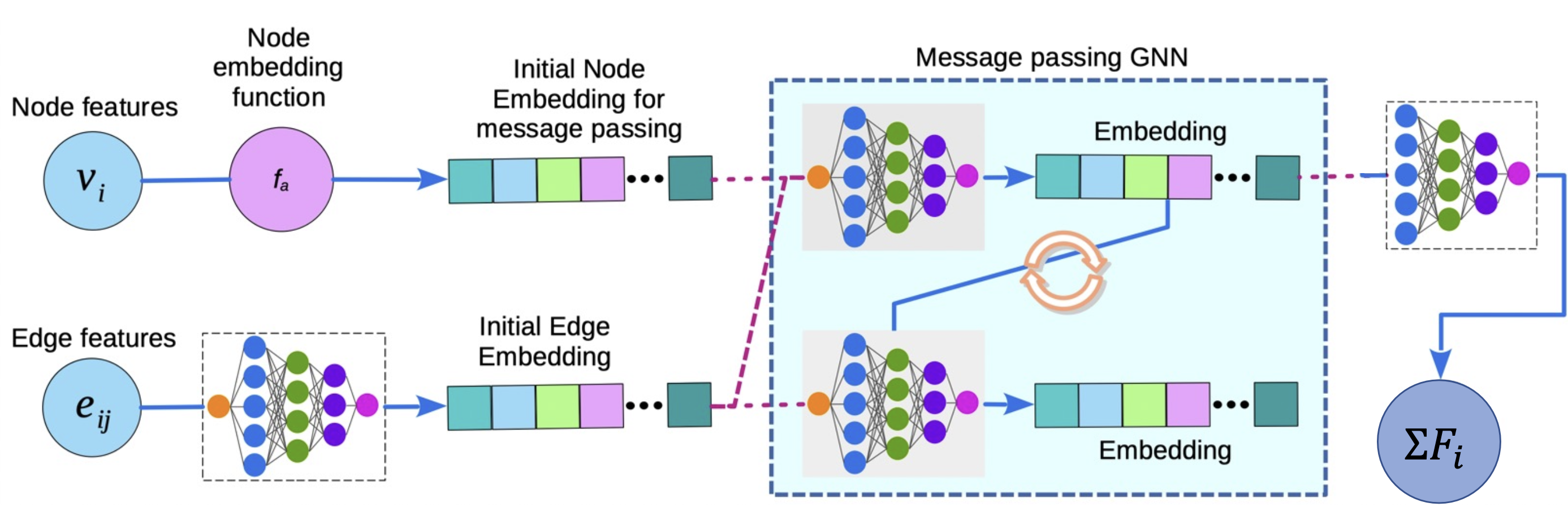
Figure 1: Graph Neural ODE architecture.

In this section, we describe the architecture of the Gnode. The graph topology is used the learn the approximate dynamics $\hat{F}$ by minimizing the loss on the predicted positions. The graph architecture is discussed in detail in the sequel.
Graph structure. An $n$-particle system is represented as a undirected graph $\mathcal{G}=\{\mathcal{V,E}\}$, where the nodes represent the particles and the edges represents the connections or interactions between them. For instance, in pendulum or springs system, the nodes correspond to bobs or balls, respectively, and the edges correspond to the bars or springs, respectively.
Input features. Each node is characterized by the features of the particles themselves, namely, the particle type ($t$), position ($q_{i}$), and velocity ($\dot{q}_{i}$). The type distinguishes particles of differing characteristics, for instance, balls or bobs with different masses. Further, each edge is represented by the edge features $w_{ij}=(q_{i}-q_{j})$, which represents the relative displacement of the nodes connected by the given edge.
Pre-Processing. In the pre-processing layer, we construct a dense vector representation for each node $v_{i}$ and edge $e_{ij}$ using $\texttt{MLP}_{em}$ as:

$$\mathbf{h}^{0}_{i} =\texttt{squareplus}(\texttt{MLP}_{em}(\texttt{one-hot}(t_{i}),q_{i},\dot{q}_{i}))$$ (6)

$$\mathbf{h}^{0}_{ij} =\texttt{squareplus}(\texttt{MLP}_{em}(w_{ij}))$$ (7)

squareplus is an activation function. Note that the $\texttt{MLP}_{em}$ corresponding to the node and edge embedding functions are parametrized with different weights. Here, for the sake of brevity, we simply mention them as $\texttt{MLP}_{em}$.
Acceleration prediction. In many cases, internal forces in a system that govern the dynamics are closely dependent on the topology of the structure. To capture this information, we employ multiple layers of message-passing between the nodes and edges. In the $l^{th}$ layer of message passing, the node embedding is updated as:

$$\mathbf{h}_{i}^{l+1}=\texttt{squareplus}\left(\mathbf{h}_{i}^{l}+\sum_{j\in\mathcal{N}_{i}}\mathbf{W}_{\mathcal{V}}^{l}\cdot\left(\mathbf{h}_{j}^{l}||\mathbf{h}_{ij}^{l}\right)\right)$$ (8)

where, $\mathcal{N}_{i}=\{v_{j}\in\mathcal{V}\mid e_{ij}\in\mathcal{E}\}$ are the neighbors of $v_{i}$. $\mathbf{W}_{\mathcal{V}}^{l}$ is a layer-specific learnable weight matrix. $\mathbf{h}_{ij}^{l}$ represents the embedding of incoming edge $e_{ij}$ on $v_{i}$ in the $l^{th}$ layer, which is computed as follows.

$$\mathbf{h}_{ij}^{l+1}=\texttt{squareplus}\left(\mathbf{h}_{ij}^{l}+\mathbf{W}_{\mathcal{E}}^{l}\cdot\left(\mathbf{h}_{i}^{l}||\mathbf{h}_{j}^{l}\right)\right)$$ (9)

Similar to $\mathbf{W}_{\mathcal{V}}^{l}$, $\mathbf{W}_{\mathcal{E}}^{l}$ is a layer-specific learnable weight matrix specific to the edge set. The message passing is performed over $L$ layers, where $L$ is a hyper-parameter. The final node and edge representations in the $L^{th}$ layer are denoted as $\mathbf{z}_{i}=\mathbf{h}_{i}^{L}$ and $\mathbf{z}_{ij}=\mathbf{h}_{ij}^{L}$ respectively. Finally, the acceleration of the particle $\ddot{q}_{i}$ is predicted as:

$$\ddot{q}_{i}=\texttt{squareplus}(\texttt{MLP}_{\mathcal{V}}(\mathbf{z}_{i}))$$ (10)

Trajectory prediction and training. Based on the predicted $\ddot{q}$, the positions and velocities are predicted using the velocity Verlet integration. The loss function of Gnode is computed by using the predicted and actual accelerations at timesteps $2,3,\ldots,\mathcal{T}$ in a trajectory $\mathbb{T}$, which is then back-propagated to train the MLPs. Specifically, the loss function is as follows.

$$\mathcal{L}=\frac{1}{n}\left(\sum_{i=1}^{n}\left(\ddot{q}_{i}^{\mathbb{T},t}-\left(\hat{\ddot{q}}_{i}^{\mathbb{T},t}\right)\right)^{2}\right)$$ (11)

Here, $(\hat{\ddot{q}}_{i}^{\mathbb{T},t})$ is the predicted acceleration for the $i^{th}$ particle in trajectory $\mathbb{T}$ at time $t$ and $\ddot{q}_{i}^{\mathbb{T},t}$ is the true acceleration. $\mathbb{T}$ denotes a trajectory from $\mathfrak{T}$, the set of training trajectories. Note that the accelerations are computed directly from the ground truth trajectory using the Verlet algorithm as:

$$\ddot{q}(t)=\frac{1}{(\Delta t)^{2}}[q(t+\Delta t)+q(t-\Delta t)-2q(t)]$$ (12)

Since the integration of the equations of motion for the predicted trajectory is also performed using the same algorithm as: $q(t+\Delta t)=2q(t)-q(t-\Delta t)+\ddot{q}(\Delta t)^{2}$, this method is equivalent to training from trajectory/positions. It should be noted that the training approach presented here may lead to learning the dynamics as dictated by the Verlet integrator. Thus, the learned dynamics may not represent the “true” dynamics of the system, but one that is optimal for the Verlet integrator.

3.2 Decoupling the dynamics and constraints (CGnode)

The proposed Gnode architecture learns the dynamics directly without decoupling the constraints and other components governing the dynamics from the equation $\ddot{q}=\hat{F}(q,\dot{q},t)$. Next, we analyze the effect of providing the constraints explicitly on the learning process and enhance the performance of Gnode. To this extent, while keeping the graph architecture exactly the same, we use Eq. 5 to compute the acceleration of the system. In this case, the output of Gnode is $N_{i}=\texttt{squareplus}(\texttt{MLP}_{\mathcal{V}}(\mathbf{z}_{i}))$ instead of $\ddot{q}_{i}$, where $N_{i}$ is the conservative force on particle $i$ (refer Eq. 2). Then, the acceleration is predicted using Eq. 5 with explicit constraints. This approach, termed as constrained Gnode (CGnode) enables us to isolate the effect of imposing constraints explicitly on the learning, and the performance of Gnode. It is worth noting that for particle systems in Cartesian coordinates, the mass matrix is a diagonal one, with the diagonal entries, $m_{ii}$s, representing the mass of the $i^{th}$ particle . Thus, the $m_{ii}$s are learned as trainable parameters. As a consequence of this design, the graph directly predicts $N_{i}$ of each particle. Since we consider a particle based system with no external force and drag, $N_{i}=\Upsilon_{i}=0$. Note that in the case of systems with drag, the graph would contain cumulative of $N_{i}$ and $\Upsilon_{i}$.

3.3 Decoupling the internal and body forces (CDGnode)

In a physical system, internal forces arise due to interactions between constituent particles. On the contrary, the body forces are due to the interaction of each particle with an external field such as gravity or electromagnetic field. While internal forces are closely related to the topology of the system, the effect of external fields on each particle is independent of the topology of the structure. In addition, while the internal forces are a function of the relative displacement between the particles, the external forces due to fields depend on the actual position of the particle.

To decouple the internal and body forces, we modify the graph architecture of the Gnode. Specifically, the node inputs are divided into local and global features. Only the local features are involved in the message passing. The global features are passed through an MLP to obtain an embedding, which is concatenated with the node embedding obtained after message passing. This updated embedding is passed through an MLP to obtain the particle level force, $N_{i}$. Here, the local node features are the particle types and the global features are position and velocity. Note that in the case of systems with drag, the $\Upsilon_{i}$ can be learned using a separate node MLP using particle type and velocity as global input features. This architecture is termed as constrained and decoupled Gnode (CDGnode). The architecture of CDGnode is provided in the Appendix.

3.4 Newton’s third law

According to Newton’s third law, “every action has an equal and opposite reaction”. In particular, the internal forces on each particle exerted by the neighboring particles should be equal and opposite so that the total system is in equilibrium. That is, $f_{ij}=-f_{ji}$, where $f_{ij}$ represents the force on particle $i$ due to its neighbor $j$. Note that this is a stronger requirement than the EL equation itself, i.e., $\frac{d}{dt}\left(\nabla_{\dot{q_{i}}}L\right)=\nabla_{q_{i}}L$. EL equation enforces that the rate of change of momentum of each particle is equal to the total force on the particle, $N_{i}=\sum_{j=1}^{n_{i}}f_{ij}$, where $n_{i}$ is the number of neighbors of $i$ — it does not enforce any restrictions on the individual component forces, $f_{ij}$ from the neighbors that add to this force. Thus, although the total force on each particle may be learned by the Gnode, the individual components may not be learned correctly. We show that Gnode with an additional inductive bias enforcing Newton’s third law, namely momentum conserving Gnode (MCGnode), conserves the linear momentum of the learned dynamics exactly.

Theorem 1

In the absence of an external field, MCGnode exactly conserves the momentum.

Proof of the theorem is provided in the Appendix A. To enforce this bias, we modify the graph architecture as follows. In particular, the output of the graph after message passing is taken from the edge embedding instead of taking from the node embedding. The final edge embedding obtained after message passing is passed through an MLP to obtain the force $f_{ij}$. Then the nodal force is computed as the sum of all the forces from the edges incident on the node. Note that while doing the sum, the symmetry condition $f_{ij}=-f_{ji}$ is enforced. Further, the global forces coming from the any external field is added separately to obtain the total nodal forces. Finally, the parameterized masses are learned as the masses in a particle system in Cartesian coordinates are diagonal in nature.

4 Empirical Evaluation

In this section, we empirically analyze the effect of each of the inductive biases on the training and performance of Gnode. First, we compare the performances of Gnode, CGnode, CDGnode, and MCGnode to elucidate the role of each of the inductive biases. Further, the best model among these is compared with the baselines as detailed below. The focus of this comparison is on the following aspects, namely, rollout and energy error, momentum error, training time and rollout time, and generalizability.

4.1 Experimental setup

$\bullet$ Simulation environment: All the simulations and training were carried out in the JAX environment [18, 19]. The graph architecture was developed using the jraph package [20]. The experiments were conducted on a machine with Apple M1 chip having 8GB RAM and running MacOS Monterey. Datasets and code base are available in the supplementary.

$\bullet$Baselines: To compare the performance of Gnode, graph-based physics-informed neural networks are considered, namely, (1) Lagrangian graph network (Lgn) [9], and (2) Hamiltonian graph network [10]. Since the exact architecture and details of the graph architecture are not provided in the original works, a full graph architecture [16, 4] is used for modeling Lgn and Hgn. Since Cartesian coordinates are used, the parameterized masses are learned as a diagonal matrix as performed in [5]. In addition, Gnode is also compared with a Node[14].

$\bullet$ Datasets and systems: To compare the performance Gnodes with different inductive biases and with the baseline models, we selected systems on which Nodes are shown to give good performance [12, 5], viz, $n$-pendulums and springs, where $n=(3,4,5)$. Further, to evaluate zero-shot generalizability of Gnode to large-scale unseen systems, we simulate 5, 20, and 50-link spring systems, and 5-, 10-, and 20-link pendulum systems. The details of the experimental systems are given in Appendix. The training data is generated for systems without drag for each particle. The timestep used for the forward simulation of the pendulum system is $10^{-5}s$ with the data collected every 1000 timesteps and for the spring system is $10^{-3}s$ with the data collected every 100 timesteps. The detailed data-generation procedure is given in the Appendix.

$\bullet$ Evaluation Metric: Following the work of [5], we evaluate performance by computing the following three error metrics, namely, (1) relative error in the trajectory, defined as the rollout error, (RE(t)), (2) Energy violation error (EE(t)), (3) relative error in momentum conservation, (ME(t)), given by:

$$RE(t)=\frac{||\hat{q}(t)-q(t)||_{2}}{||\hat{q}(t)||_{2}+||q(t)||_{2}},\quad EE(t)=\frac{||\hat{\mathcal{H}}-\mathcal{H}||_{2}}{(||\hat{\mathcal{H}}||_{2}+||\mathcal{H}||_{2}},\quad ME(t)=\frac{||\hat{\mathcal{M}}-\mathcal{M}||_{2}}{||\hat{\mathcal{M}}||_{2}+||\mathcal{M}||_{2}}$$ (13)

Note that all the variables with a hat, for example $\hat{x}$, represent the predicted values based on the trained model and the variables without hat, that is $x$, represent the ground truth.

$\bullet$ Model architecture and training setup: For all versions of Gnode, Lgn, and Hgn, the MLPs are two-layers deep. We use 10000 data points generated from 100 trajectories to train all the models. This dataset is divided randomly in 75:25 ratio as training and validation set. All models were trained till the decrease in loss saturates to less than 0.001 over 100 epochs. The model performance is evaluated on a forward trajectory, a task it was not explicitly trained for, of $10s$ in the case of pendulum and $20s$ in the case of spring. Note that this trajectory is  2-3 orders of magnitude larger than the training trajectories from which the training data has been sampled. The dynamics of $n$-body system is known to be chaotic for $n\geq 2$. Hence, all the results are averaged over trajectories generated from 100 different initial conditions.

4.2 Evaluation of inductive biases in Gnode

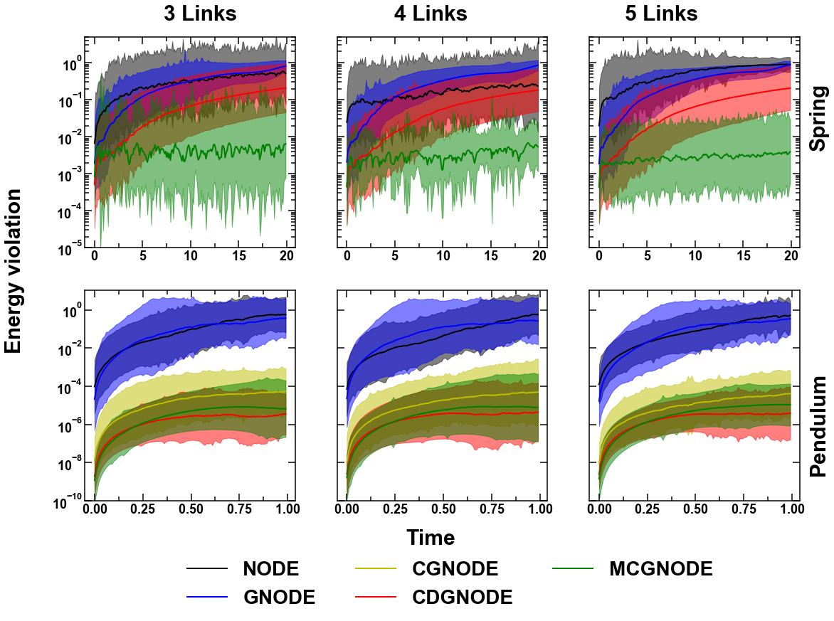
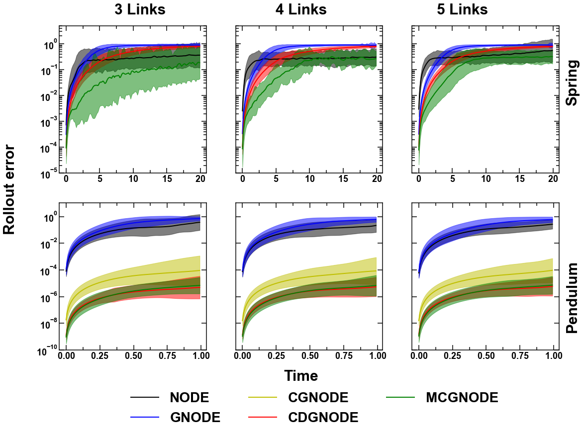
Figure 2: Comparison of the energy violation and rollout error between Node, Gnode, CGnode, CDGnode, MCGnode for $n$-pendulum and spring systems with $n=3,4,5$ links. For the pendulum system, model is trained on 3-pendulum system and for the spring system, model is trained on the 5-spring system and evaluated on all other systems. Shaded region shows the 95% confidence interval from 100 initial conditions.

First, we focus on empirically evaluating the contribution of the different inductive biases discussed in Section 3 on the performance of Node.

$\bullet$ Performance of (Gnode): Figure 2 shows the performance of Gnode  on pendulum and spring systems of sizes 3 to 5. The Gnode for pendulum is trained on a 3-pendulum system and that of spring is trained on a 5-spring system. Hence, the 4- and 5-pendulum systems and 3- and 4-spring systems are unseen, and consequently, allows us to evaluate zero-shot generalizability. We observe that energy violation and rollout errors of Gnode for the forward simulations are comparable, both in terms of the value and trend with respect to time, across all of the systems. This confirms the generalizability of Gnode to simulate the dynamics of unseen systems of arbitrary sizes.

$\bullet$ Impact of topology: To precisely measure the impact of topology, in 5-pendulum and 5-spring systems, we also include Node as a baseline in Fig. 2. When we compare Node with Gnode, we observe that while they are comparable in 5-pendulum, Gnode is better in 5-spring. In addition, Gnode is inductive due to training on node level dynamics, while Node is not. It is therefore worth highlighting that Node has an unfair advantage on 5-pendulum since it is trained and tested on the same system, while 5-pendulum is unseen for Gnode (trained on 3-pendulum). Overall, it is safe to say that topology helps; the inductive biased infused due to topology leads to comparable or lower error, while also imparting zero-shot generalizability. In the appendix, we provide more experiments comparing Node with Gnode to further highlight the benefit of topology-aware modeling.

$\bullet$ Gnode with explicit constraints (CGnode): Next, we analyze the effect of incorporating the constraints explicitly in Gnode. To this extent, we train the 3-pendulum system using CGnode model with acceleration computed using Equation 5. Further, we evaluate the performance of the model on 4- and 5-pendulum systems. Note that the spring system is an unconstrained system and hence CGnode is equivalent to Gnode for this system. We observe that (see Fig. 2) CGnode exhibits $\sim$4 orders of magnitude superior performance both in terms of energy violation and rollout error. This confirms that providing explicit constraints significantly improves both the learning efficiency and the predictive dynamics of Gnode models where explicit constraints are present, for example, pendulum systems, chains or rigid bodies.

$\bullet$ Decoupling internal and body forces (CDGnode): Now, we analyze the effect of decoupling local and global features in the Gnode by employing the CDGnode architecture. It is worth noting that the decoupling the local and global features makes the Gnode model parsimonious with only the relative displacement and node type given as input features for message passing to the graph architecture. In other words, the number of features give to the graph architecture is lower in CDGnode in Gnode. Interestingly, we observe that the CDGnode performs better than CGnode and Gnode by $\sim$1 order of magnitude for pendulum and spring systems, respectively.

$\bullet$ Newton’s third law (MCGnode): Finally, we empirically evaluate the effect of enforcing Newton’s third law, that is, $f_{ij}=-f_{ji}$ on the graph using the graph architecture namely, MCGnode. Figure 2 shows the performance of MCGnode for both pendulum and spring systems. Note that it was theoretically demonstrated that this inductive bias enforces the exact conservation of momentum, in the absence of an external field. Figure 4 shows the $ME$ (see Equation 13) of MCGnode in comparison to Node, Gnode, CGnode, CDGnode, and MCGnode for pendulum and spring systems. We observe that in the spring system the $ME$ of MCGnode is zero. In the case of a pendulum, although lower than Node, Gnode, and CGnode, the $ME$ of MCGnode is comparable to that of CDGnode. Correspondingly, MCGnode exhibits improved performance for the spring system in comparison to other models. However, in pendulum system, we observe that the performance of MCGnode is similar to that of CDGnode. This is because in spring systems, the internal forces between the balls govern the dynamics of the system, whereas in pendulum the dynamics is governed mainly by the force exerted on the bobs by the external gravitational field. Interestingly, we observe that the energy violation error of MCGnode remains fairly constant, while this error diverges for other models. This confirms that a strong enforcement of momentum conservation in turn ensures that the energy violation error stays constant over time, ensuring a stable long-term equilibrium dynamics of the system. MCGnode will, thus, be particularly useful for the statistical analysis of chaotic systems where multiple divergent trajectories correspond to the same energy state.

4.3 Comparison with baselines

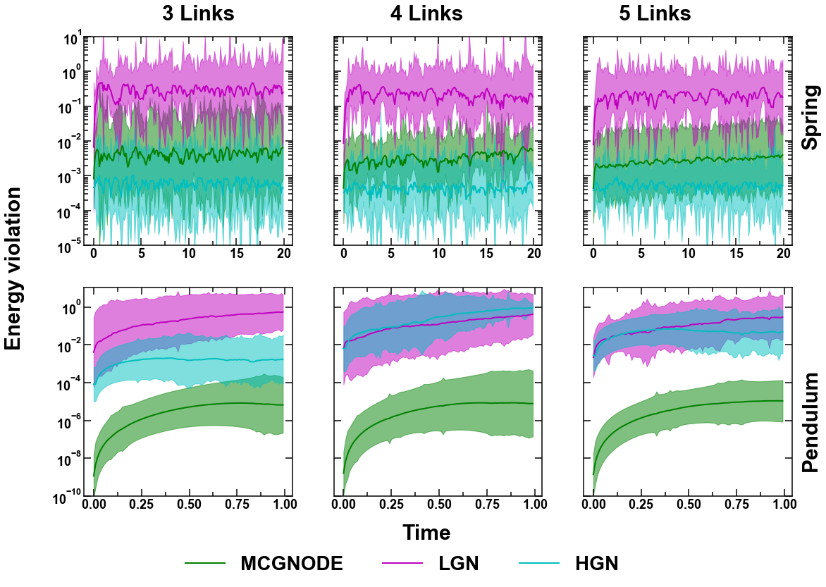
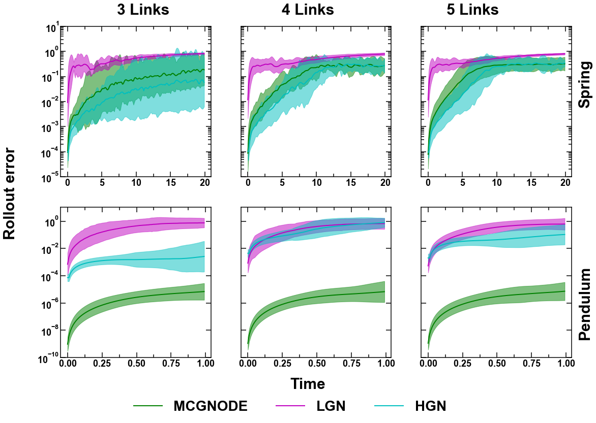
Figure 3: Comparison of the energy violation and rollout error between Gnode, Lgn, and Hgn for $n$-pendulum and spring systems with $n=3,4,5$ links. For both the pendulum and spring systems, the model is trained on 5-link structure and evaluated on all other systems. Shaded region shows the 95% confidence interval from 100 initial conditions.

Now, we compare the Gnode that exhibited the best performance, namely, MCGnode with the baselines namely, Lgn and Hgn. Note that both Lgn and Hgn are energy conserving graph neural networks, which are expected to give superior performance in predicting the trajectories of dynamical systems [10]. Especially, due to their energy conserving nature, these models are expected to have lower energy violation error than other models, where energy conservation bias is not explicitly enforced. Figure 3 shows the energy violation and rollout error of Gnode, Lgn, and Hgn trained on 5-link system and tested on 3, 4, 5-link pendulum and spring systems. Interestingly, we observe that MCGnode outperforms both Lgn and Hgn in terms of rollout error and energy error for both spring and pendulum systems. Specifically, in case of pendulum systems, we observe that the energy violation and rollout errors are $\sim 5$ orders of magnitude lower in the case of MCGnode in comparison to Lgn and Hgn. Further, we compare the $ME$ of MCGnode with Lgn and Hgn (see Fig. 4 right palette). We observe in both pendulum and spring systems that the $ME$ of MCGnode is significantly lower than that of Lgn and Hgn. Thus, in the case of spring systems, although the performance of Hgn and MCGnode are comparable for both $RE$ and $EE$, we observe that MCGnode exhibits zero in $ME$, while in Hgn and Lgn $ME$ diverges.

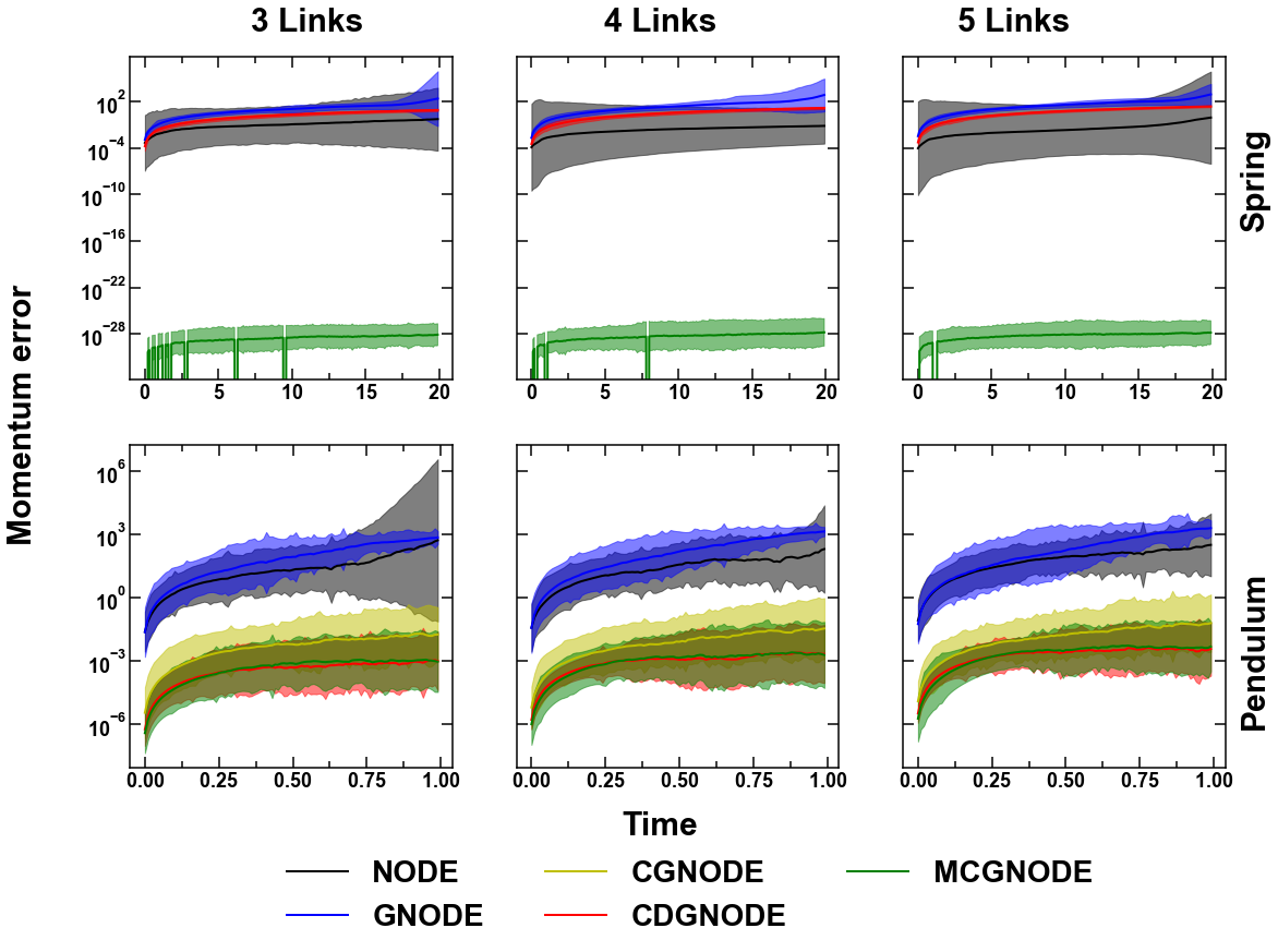
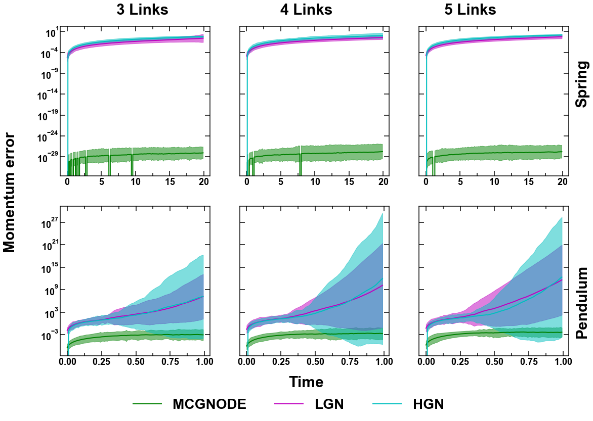
Figure 4: Momentum error ($ME$) of Node, Gnode, CGnode, CDGnode, and MCGnode (top palette), and Lgn, Hgn, MCGnode (bottom palette) for spring (top row of both the palettes) and pendulum (bottom row of both the palettes) systems with 3, 4, and 5 links. The shaded region represents the 95% confidence interval based on 100 forward simulations.

4.4 Generalizability

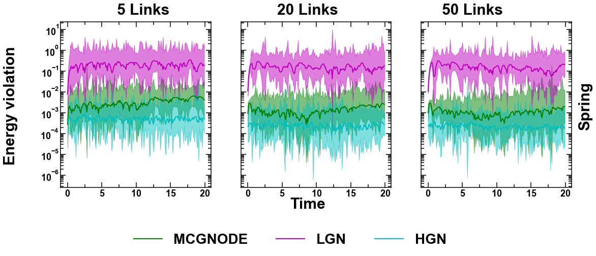
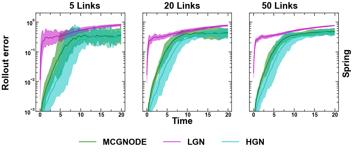
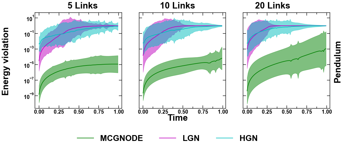
Figure 5: Energy violation and rollout error between Gnode, Lgn, and Hgn for spring systems with $5,20,50$ links and pendulum system with $5,10,20$ links. Note that for all the systems, Gnode, Lgn and Hgn are trained on 3-pendulum and 5-spring systems and tested on others. The shaded region represent the $95\%$ confidence interval based on $100$ forward simulations.

Now, we focus on the zero-shot generalizability of Gnode, Lgn, and Hgn to large systems that are unseen by the model. To this extent, we model 5-, 10-, and 20-link pendulum systems and 5-, 20-, 50-link spring systems. Note that all the models are trained on the 5-link systems. In congruence with the comparison earlier, we observe that MCGnode performs better than both Lgn and Hgn, when tested on systems with large number of links. However, we observe that the variation in the error represented by the 95% confidence interval increases with increase in the number of particles. This suggests that the increase in the number of particles essentially results in an increased noise in the prediction of the forces. However, error in the Gnode is significantly lower than the error in Lgn and Hgn for both pendulum and spring systems, as confirmed by the 95% confidence interval. This suggests that MCGnode can generalize to larger system sizes with increased accuracy.

4.5 Learning the dynamics of 3D solid

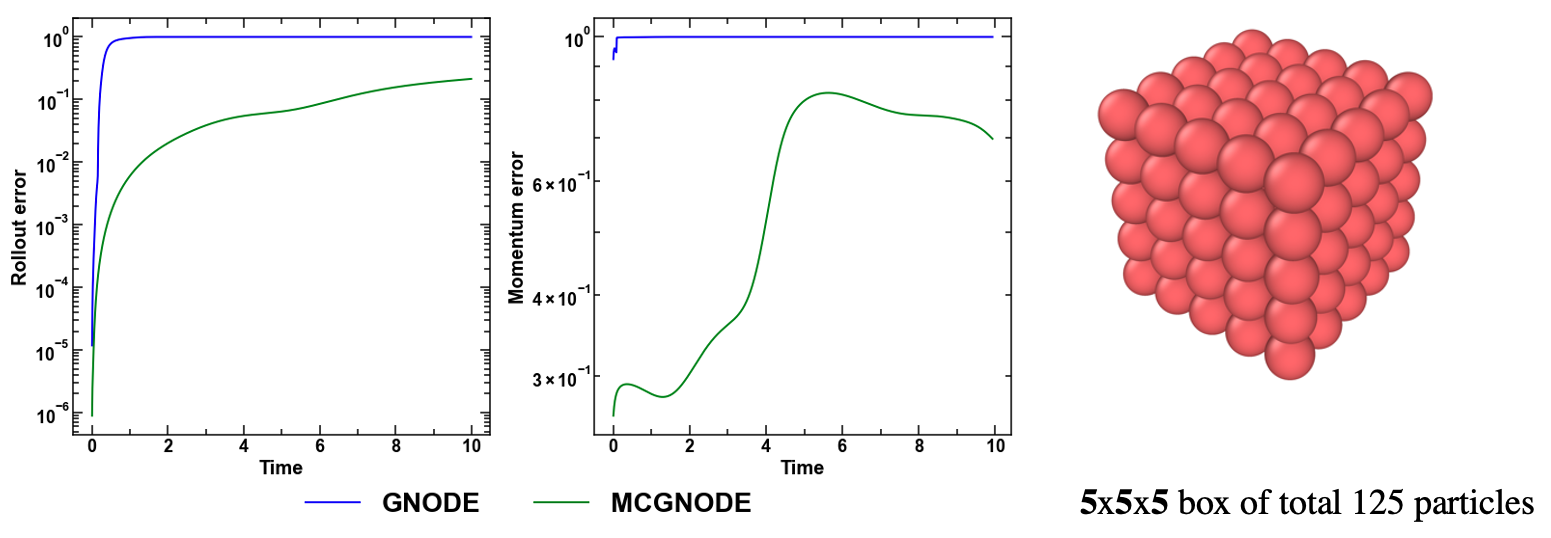
Figure 6: ($RE$) and ($ME$) of Gnode, and MCGnode for particle-based system. Here original simulation is performed using peridynamics on a 3D box of $125$ particle ($5\times 5\times 5$).

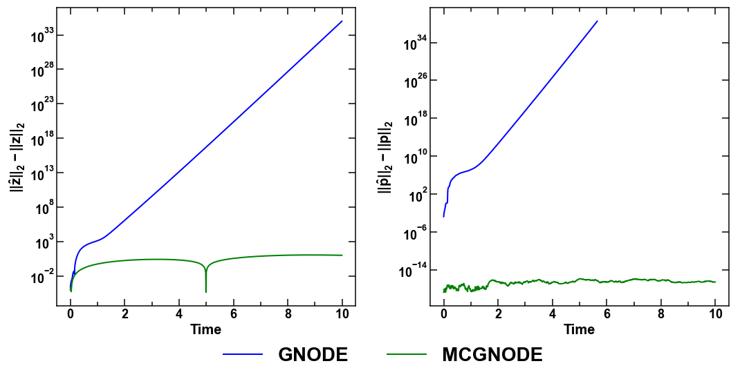
Figure 13: Absolute trajectory error error and absolute momentum error for peridynamics simulation using of GNODE, and MCGNODE.

To demonstrate the applicability of MCGNODE to learn the dynamics of complex systems, we consider a challenging problem, that is, inferring the dynamics of an elastically deformable body. Specifically, a $5\times 5\times 5$ solid cube, discretized into $125$ particles, is used for simulating the ground truth. 3D solid system is simulated using the peridynamics framework. The system is compressed isotropically and then released to simulate the dynamics of the solid, that is, the contraction and expansion in 3D. We observe that MCGNODE learns the dynamics of the system and perform inference much superior to GNODE (see Fig. 6). It should also be noted that although the momentum error in MCGNODE seems high, this is due to the fact that the actual momentum in these systems are significantly low. This is demonstrated by plotting the absolute momentum error in these systems which in MCGNODE is close to zero, while in GNODE it explodes (see Fig. 13). These results suggest that the MCGNODE presented here could be applied much more complex systems such as solids or other particle-based systems where momentum conservation is equally important as energy conservation.

5 Conclusions

In this work, we carefully analyze various inductive biases that can affect the performance of a Gnode. Specifically, we analyze the effect of a graph architecture, explicit constraints, decoupling global and local features that makes the model parsimonious, and Newton’s third law that enforces a stronger constraint on the conservation of momentum. We observe that inducing appropriate inductive biases results in an enhancement in the performance of Gnode by $\sim$2-3 orders magnitude for spring systems and $\sim$5-6 orders magnitude for pendulum systems in terms of energy violation error. Further, the Gnode that exhibits superior performance, namely MCGnode, outperforms the graph versions of both Lagrangian and Hamiltonian neural networks, namely, Lgn and Hgn. Altogether, the present work suggests that the performance of Gnode-based models can be enhanced and even made superior to energy conserving neural networks by inducing the appropriate inductive biases.

Limitations and Future Works: At this juncture, it is worth mentioning some of the limitations of the present work that may be addressed as part of future works. The present work focuses on particle-based systems such as pendulum and spring systems. While these simple systems can be used to evaluate model performances, real-life are more complex in nature with rigid body motions, contacts, and collisions. Extending Gnode to address these problems can enable modeling of realistic systems. A more complex set of systems involve plastically deformable systems such as steel rod, and viscoelastic materials where the deformation depends on the strain rate of materials. From the neural modeling perspective, the Gnode is essentially a graph convolutional network. Currently, messages from all neighbors are treated as equally important. Using attention over each message passing head may allow us to better differentiate neighbors based on the strength of their interactions. We hope to pursue these questions in the future.

Appendix A Proof of Theorem 1

Proof. Consider a system without any external field where the dynamics is governed by internal forces, for instance, a $n$-spring system. The conservation of linear momentum for this system implies that $\sum_{i=1}^{n}\frac{d}{dt}\left(\hat{m}_{ii}\hat{\dot{q}}_{i}\right)=0$, where $\hat{\dot{q}}_{i}$ represents the predicted velocity, $\hat{m}_{ii}$ represents the learned mass of the particle $i$, and $\dot{q}_{i}$ represents the ground truth velocity. Assume the error in the rate of change of momentum of the predicted trajectory to be $\hat{\varepsilon}_{t}$. To prove that MCGnode conserves the momentum exactly, it is sufficient to prove that $\hat{\varepsilon}_{t}=0$. Consider,

$$\hat{\varepsilon}_{t} =\sum_{i=1}^{n}\hat{\varepsilon}_{i,t}=\sum_{i=1}^{n}\frac{d}{dt}\left(\hat{m}_{ii}\hat{\dot{q}}_{i}-m_{ii}\dot{q}_{i}\right)=\sum_{i=1}^{n}(\hat{N}_{i}-N_{i})=\sum_{i=1}^{n}\hat{N}_{i}-\sum_{i=1}^{n}N_{i}$$ (14)

Note that in equation 3, all terms except $N_{i}$ are either known or are zero. Thus, without loss of generality, $\sum_{i=1}^{n}N_{i}=0$, in the absence of an external field. Hence,

$$\hat{\varepsilon}_{t} =\sum_{i=1}^{n}\hat{\varepsilon}_{i,t}=\sum_{i=1}^{n}\hat{N}_{i}=\sum_{i=1}^{n}\sum_{j=1}^{n_{i}}f_{ij}=\sum_{i=1}^{n}\sum_{j=1}^{n_{i}}\frac{(f_{ij}+f_{ji})}{2}$$ (15)

The inductive bias $f_{ij}=-f_{ji}$ implies that $\frac{(f_{ij}+f_{ji})}{2}=0$. Thus,

$$\sum_{i=1}^{n}\frac{d}{dt}\left(m_{ii}\hat{\dot{q}}_{i}\right)=\hat{\varepsilon}_{t}=0\hskip 72.26999pt\square$$

Appendix B Impact of topology: Node vs Gnode vs MCGnode

To evaluate the impact of topology in detail, we compare the performance of Node, Gnode, MCGnode in Figure 7. In the case of Node, the system is trained and evaluated on each of the pendulum and spring systems separately. In the case of Gnode and MCGnode, the training is performed on 5-spring and 3-pendulum system and evaluated on all other systems. First, we observe that the performance of Node and Gnode are comparable for both rollout and energy error. This suggests that the performance of Gnode, with no additional inductive bias, is comparable to that of Node with the additional advantage that Gnode can generalize to any system size. Now, we compare the performance of Node with MCGnode, which has all the additional inductive biases discussed earlier. We observe that MCGnode performs significantly better than Node, as expected. It is worth noting that while the inductive bias of explicit constraints can be infused in Node in a similar fashion as in Gnode, other inductive biases such as decoupling the global and local features and Newton’s third law are unique to the graph structure. These inductive biases cannot be infused in a Node structure. This, in turn, demonstrates the superiority of Gnode which allows additional inductive biases due to the explicit representation of the topology through the graph structure.

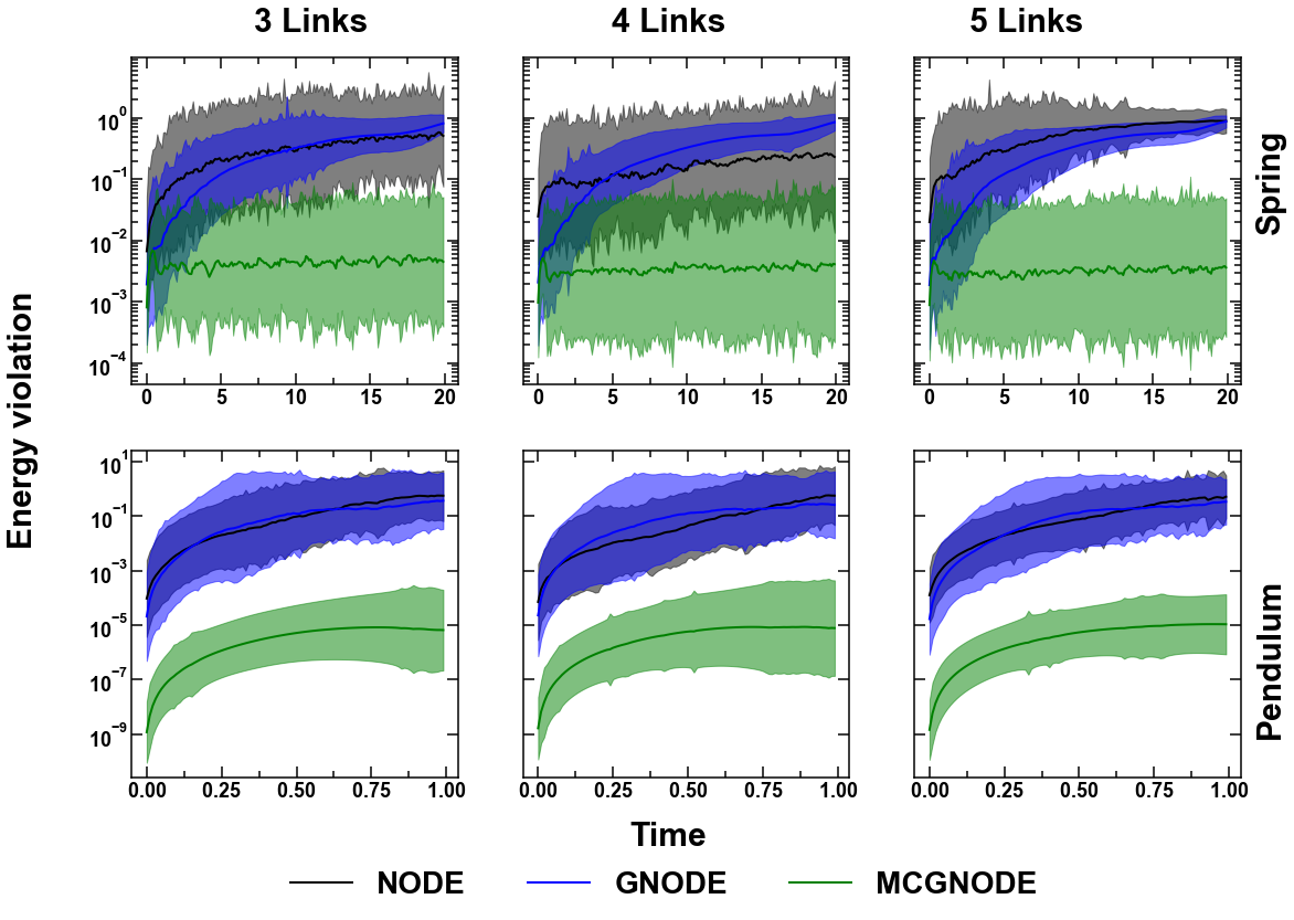
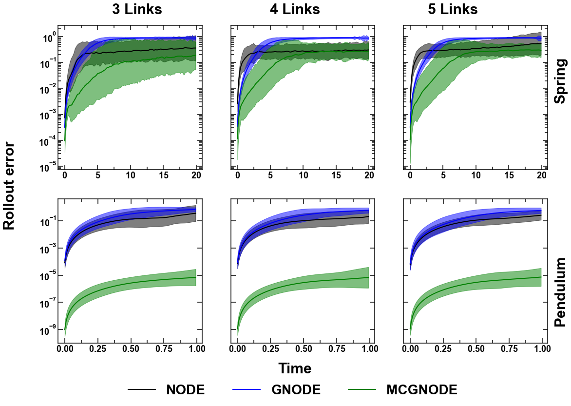
Figure 7: Energy error and trajectory error for Node, Gnode, and MCGnode for spring and pendulum systems with 3-,4-, and 5-links. The shaded region represents the 95% confidence interval based on 100 forward simulations.

Appendix C Training efficiency

Here, we compare the training efficiency of MCGnode with the Node. Specifically, we focus on the best graph-based architecture and compare the performance with the baseline Node 5-spring and 3-pendulum systems. Figure 8 shows the performance of MCGnode in comparison to Node for the dataset sizes of 100, 500, 1000, 5000, and 10000 in terms of the geometric mean of the energy error and rollout error. We observe that the learning of MCGnode is significantly simplified in comparison to that of Node—MCGnode exhibits orders of magnitude better performance in terms of both energy and rollout error for both pendulum and spring systems.

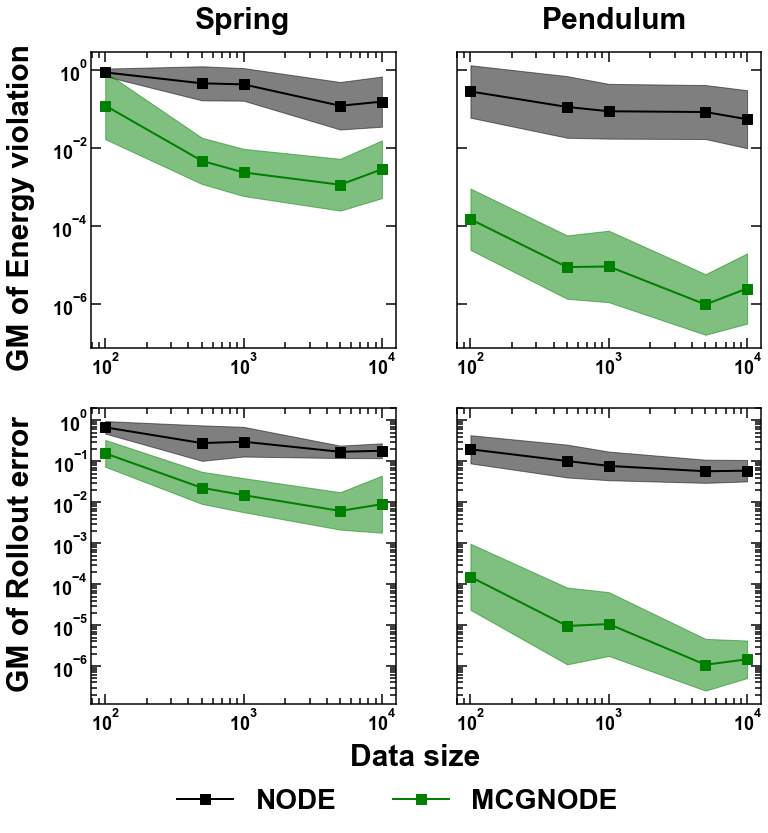
Figure 8: Training efficiency of MCGnode in comparison with the Gnode. The shaded region represents the 95% confidence interval based on 100 forward simulations.

Appendix D Experimental systems

D.1 $n$-Pendulum

In an $n$-pendulum system, $n$-point masses, representing the bobs, are connected by rigid bars which are not deformable. These bars, thus, impose a distance constraint between two point masses as

$$||q_{i}-q_{i-1}||=l_{i}$$ (16)

where, $l_{i}$ represents the length of the bar connecting the $(i-1)^{th}$ and $i^{th}$ mass. This constraint can be differentiated to write in the form of a Pfaffian constraint as

$$q_{i}\dot{q}_{i}+q_{i-1}\dot{q}_{i-1}=0$$ (17)

Note that such constraint can be obtained for each of the $n$ masses considered to obtain the $A(q)$.

The mass of each of the particles is $m_{i}$ and the force on each bob due to the acceleration due to gravity in $m_{i}g$. This force will be compensated by the constraint forces, which in turn governs the motion of the pendulum. For Lgn, the Lagrangian of this system has contributions from potential energy due to gravity and kinetic energy. Thus, the Lagrangian can be written as

$$\mathcal{L}=\sum_{i=1}^{n}\left(1/2m_{i}\dot{q_{i}}^{\texttt{T}}\dot{q_{i}}-m_{i}gy_{i}\right)$$ (18)

And, for Hgn, the Hamiltonian is given by

$$\mathcal{H}=\sum_{i=1}^{n}\left(1/2m_{i}\dot{q_{i}}^{\texttt{T}}\dot{q_{i}}+m_{i}gy_{i}\right)$$ (19)

where $g$ represents the acceleration due to gravity in the $y$ direction.

D.2 $n$-spring system

In this system, $n$-point masses are connected by elastic springs that deform linearly with extension or compression. Note that similar to a pendulum setup, each mass $m_{i}$ is connected only to two masses $m_{i-1}$ and $m_{i+1}$ through springs so that all the masses form a closed connection. Thus, the force experienced by each bob $i$ due to a spring connecting $i$ to its neighbor $j$ is $f_{ij}=1/2k(||q_{i}-q_{j}||-r_{i})$. For Lgn, the Lagrangian of this system is given by

$$\mathcal{L}=\sum_{i=1}^{n}1/2m_{i}\dot{q_{i}}^{\texttt{T}}\dot{q_{i}}-\sum_{i=1}^{n}1/2k(||q_{i-1}-q_{i}||-r_{0})^{2}$$ (20)

And,for Hgn, the Hamiltonian by:

$$\mathcal{H}=\sum_{i=1}^{n}1/2m_{i}\dot{q_{i}}^{\texttt{T}}\dot{q_{i}}+\sum_{i=1}^{n}1/2k(||q_{i-1}-q_{i}||-r_{0})^{2}$$ (21)

where $r_{0}$ and $k$ represent the undeformed length and the stiffness, respectively, of the spring.

Appendix E Implementation details

E.1 Dataset generation

Software packages: numpy-1.22.1, jax-0.3.0, jax-md-0.1.20, jaxlib-0.3.0, jraph-0.0.2.dev
Hardware: Chip: Apple M1, Total Number of Cores: 8 (4 performance and 4 efficiency), Memory: 8 GB, System Firmware Version: 7459.101.3, OS Loader Version: 7459.101.3

For NODE, all versions of GNODE, LGN: All the datasets are generated using the known Lagrangian of the pendulum and spring systems, along with the constraints, as described in Section D. For each system, we create the training data by performing forward simulations with 100 random initial conditions. For the pendulum system, a timestep of $10^{-5}s$ is used to integrate the equations of motion, while for the spring system, a timestep of $10^{-3}s$ is used. The velocity-Verlet algorithm is used to integrate the equations of motion due to its ability to conserve the energy in long trajectory integration.

While for HGN, datasets are generated using Hamiltonian mechanics. Runge-Kutta integrator is used to integrate the equations of motion due to the first order nature of the Hamiltonian equations in contrast to the second order nature of Lgn, Node, and all versions of Gnode.

From the 100 simulations for pendulum and spring system, obtained from the rollout starting from 100 random initial conditions, 100 data points are extracted per simulation, resulting in a total of 10000 data points. Data points were collected every 1000 and 100 timesteps for the pendulum and spring systems, respectively. Thus, each training trajectory of the spring and pendulum systems are $10s$ and $1s$ long, respectively. Here, we do not train from the trajectory. Rather, we randomly sample different states from the training set to predict the acceleration.

E.2 Architecture

For Node, we use a fully connected feed-forward neural network with 2 hidden layers, each having 16 hidden units with a square-plus activation function. For all versions of Gnode, graph architecture is used with each MLP consisting of two layers with 5 hidden units. One round of message passing is performed for both pendulum and spring. For Lgn and Hgn, full graph architecture is used with each MLPs consist of two layers with 16 hidden units and one round of message passing were performed. The hyperparameters were optimized based on the good practices of the model development.

E.3 Architecture of CDGNODE

Figure 9 shows the architecture of the CDGnode. Note that an external MLP associated with the global features are included in addition to the graph architecture.

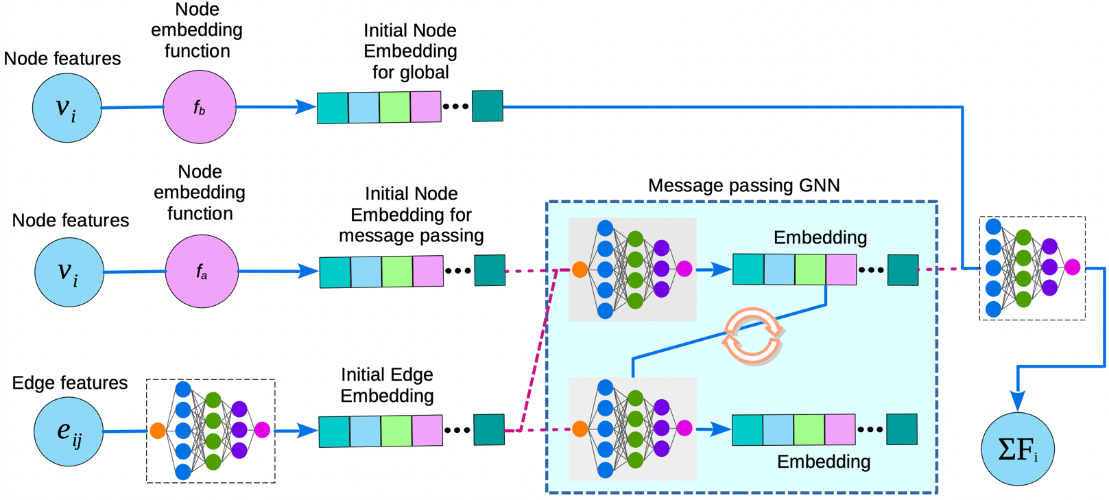
Figure 9: CDGNODE Architecture.

E.4 Edge features: position vs velocity

Figure 10 shows the loss curve with relative position and relative velocity as edge features. We observe that when relative velocity is provided as the edge feature, model struggles to learn and saturates quickly.

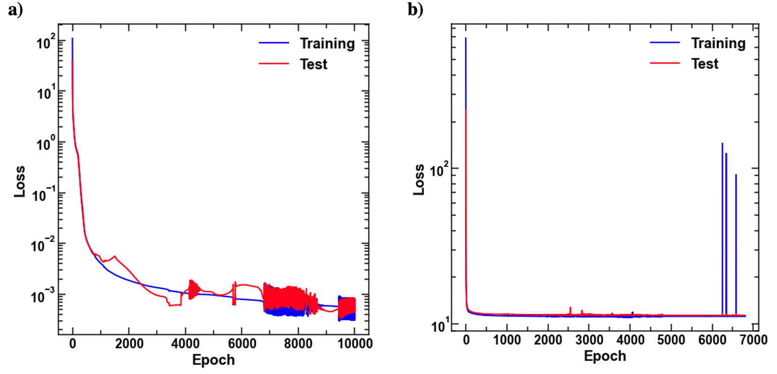
Figure 10: Loss curve when (a) relative position is used as edge feature and (b) relative velocity is used as edge feature.

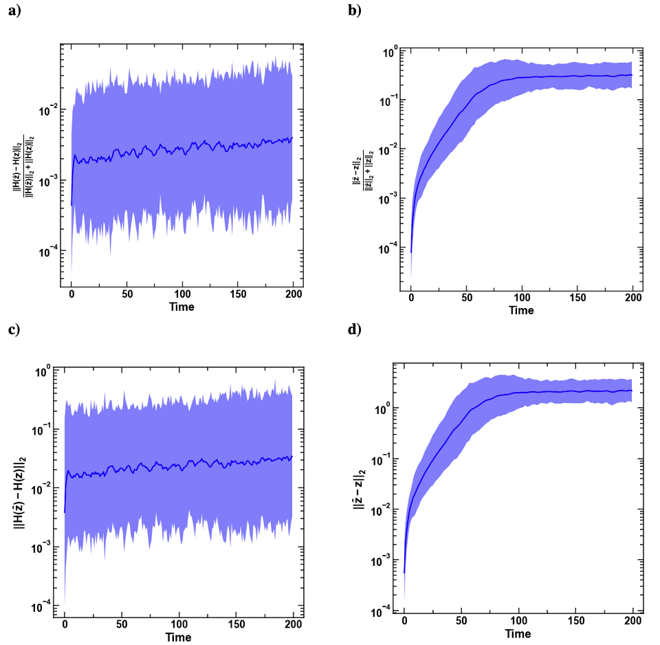
Figure 11: Plot comparing (a) relative energy error, (b) relative trajectory error, (c) absolute energy error, (d) absolute trajectory error for the 5-Spring-MCGNODE system

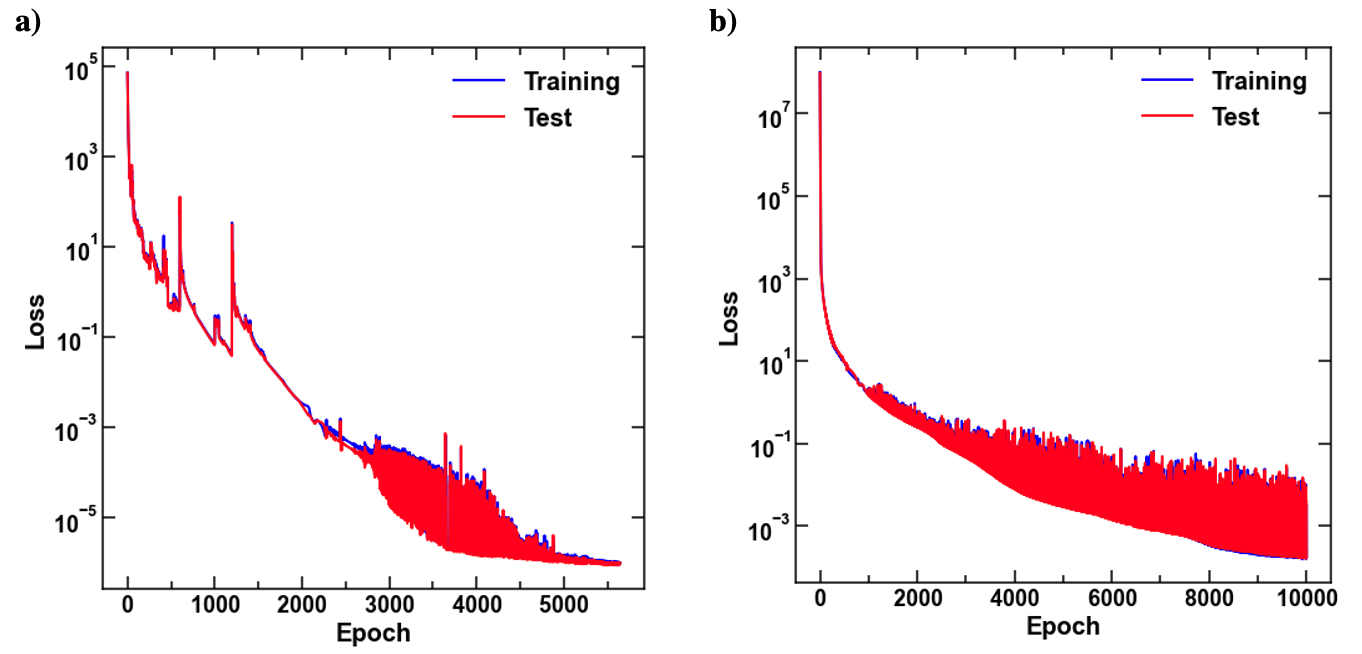
Figure 12: Loss curve for peridynamics system using (a) MCGNODE architecture and (b) GNODE architecture.

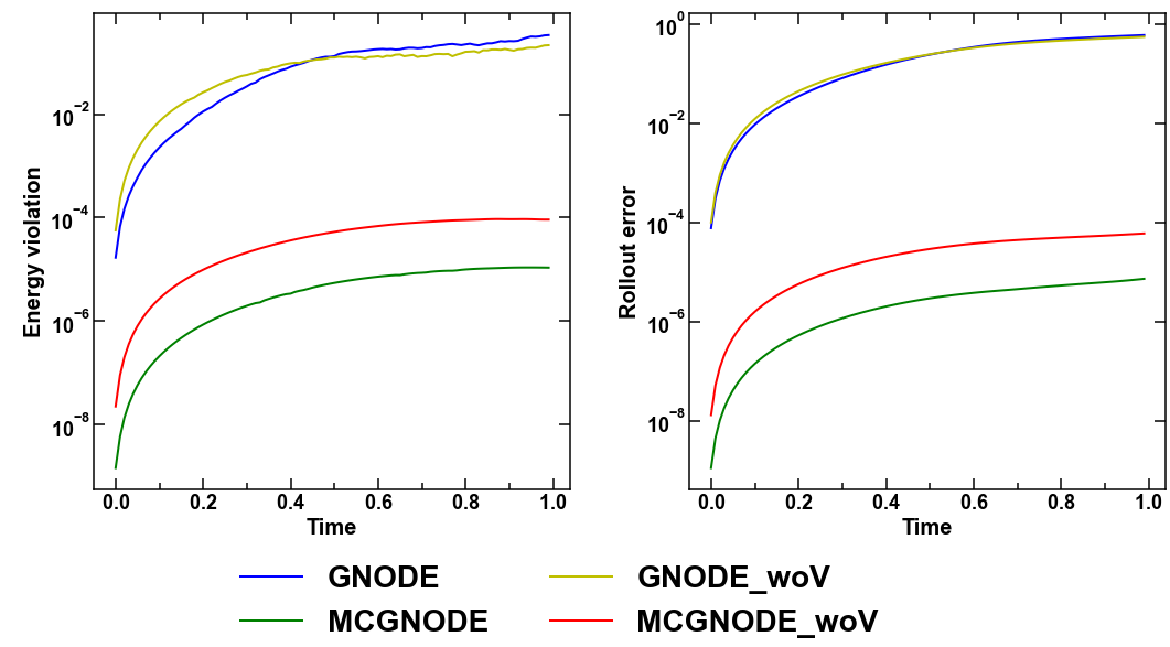
Figure 14: Comparison of Energy violation and rollout error for 5-link pendulum using GNODE, MCGNODE, GNODEwoV (GNODE without velocity as input) and MCGNODEwoV (MCGNODE without velocity as input).

E.5 Training details

The training dataset is divided in 75:25 ratio randomly, where the 75% is used for training and 25% is used as the validation set. Further, the trained models are tested on its ability to predict the correct trajectory, a task it was not trained on. Specifically, the pendulum systems are tested for $1s$, that is $10^{5}$ timesteps, and spring systems for $20s$, that is $2\times 10^{4}$ timesteps on 100 different trajectories created from random initial conditions. All models are trained for 10000 epochs. A learning rate of $10^{-3}$ was used with the Adam optimizer for the training.

$\bullet$NODE

Parameter	Value
Hidden layer neurons (MLP)	16
Number of hidden layers (MLP)	2
Activation function	squareplus
Optimizer	ADAM
Learning rate	$1.0e^{-3}$
Batch size	100

$\bullet$GNODE, CGNODE, CDGNODE, MCGNODE

Parameter	Value
Node embedding dimension	5
Edge embedding dimension	5
Hidden layer neurons (MLP)	5
Number of hidden layers (MLP)	2
Activation function	squareplus
Number of layers of message passing	1
Optimizer	ADAM
Learning rate	$1.0e^{-3}$
Batch size	100

$\bullet$LGN, HGN

Parameter	Value
Node embedding dimension	8
Edge embedding dimension	8
Hidden layer neurons (MLP)	16
Number of hidden layers (MLP)	2
Activation function	squareplus
Number of layers of message passing	1
Optimizer	ADAM
Learning rate	$1.0e^{-3}$
Batch size	100

References

- [1] Steven M LaValle. Planning algorithms. Cambridge university press, 2006.
- [2] Herbert Goldstein. Classical mechanics. Pearson Education India, 2011.
- [3] Yaofeng Desmond Zhong, Biswadip Dey, and Amit Chakraborty. Dissipative symoden: Encoding hamiltonian dynamics with dissipation and control into deep learning. arXiv preprint arXiv:2002.08860, 2020.
- [4] Alvaro Sanchez-Gonzalez, Jonathan Godwin, Tobias Pfaff, Rex Ying, Jure Leskovec, and Peter Battaglia. Learning to simulate complex physics with graph networks. In International Conference on Machine Learning, pages 8459–8468. PMLR, 2020.
- [5] Marc Finzi, Ke Alexander Wang, and Andrew G Wilson. Simplifying hamiltonian and lagrangian neural networks via explicit constraints. In H. Larochelle, M. Ranzato, R. Hadsell, M. F. Balcan, and H. Lin, editors, Advances in Neural Information Processing Systems, volume 33, pages 13880–13889. Curran Associates, Inc., 2020.
- [6] George Em Karniadakis, Ioannis G Kevrekidis, Lu Lu, Paris Perdikaris, Sifan Wang, and Liu Yang. Physics-informed machine learning. Nature Reviews Physics, 3(6):422–440, 2021.
- [7] Michael Lutter, Christian Ritter, and Jan Peters. Deep lagrangian networks: Using physics as model prior for deep learning. In International Conference on Learning Representations, 2019.
- [8] Ziming Liu, Yuanqi Du, Yunyue Chen, and Max Tegmark. Physics-augmented learning: A new paradigm beyond physics-informed learning. In NeurIPS 2021 AI for Science Workshop, 2021.
- [9] Miles Cranmer, Sam Greydanus, Stephan Hoyer, Peter Battaglia, David Spergel, and Shirley Ho. Lagrangian neural networks. In ICLR 2020 Workshop on Integration of Deep Neural Models and Differential Equations, 2020.
- [10] Alvaro Sanchez-Gonzalez, Victor Bapst, Kyle Cranmer, and Peter Battaglia. Hamiltonian graph networks with ode integrators. arXiv e-prints, pages arXiv–1909, 2019.
- [11] Samuel Greydanus, Misko Dzamba, and Jason Yosinski. Hamiltonian neural networks. Advances in Neural Information Processing Systems, 32:15379–15389, 2019.
- [12] Yaofeng Desmond Zhong, Biswadip Dey, and Amit Chakraborty. Benchmarking energy-conserving neural networks for learning dynamics from data. In Learning for Dynamics and Control, pages 1218–1229. PMLR, 2021.
- [13] Ricky TQ Chen, Yulia Rubanova, Jesse Bettencourt, and David Duvenaud. Neural ordinary differential equations. In Proceedings of the 32nd International Conference on Neural Information Processing Systems, pages 6572–6583, 2018.
- [14] Nate Gruver, Marc Anton Finzi, Samuel Don Stanton, and Andrew Gordon Wilson. Deconstructing the inductive biases of hamiltonian neural networks. In International Conference on Learning Representations, 2021.
- [15] Franco Scarselli, Marco Gori, Ah Chung Tsoi, Markus Hagenbuchner, and Gabriele Monfardini. The graph neural network model. IEEE transactions on neural networks, 20(1):61–80, 2008.
- [16] Miles Cranmer, Alvaro Sanchez Gonzalez, Peter Battaglia, Rui Xu, Kyle Cranmer, David Spergel, and Shirley Ho. Discovering symbolic models from deep learning with inductive biases. Advances in Neural Information Processing Systems, 33, 2020.
- [17] Richard M Murray, Zexiang Li, and S Shankar Sastry. A mathematical introduction to robotic manipulation. CRC press, 2017.
- [18] Samuel Schoenholz and Ekin Dogus Cubuk. Jax md: a framework for differentiable physics. Advances in Neural Information Processing Systems, 33, 2020.
- [19] James Bradbury, Roy Frostig, Peter Hawkins, Matthew James Johnson, Chris Leary, Dougal Maclaurin, and Skye Wanderman-Milne. Jax: composable transformations of python+ numpy programs, 2018. URL http://github. com/google/jax, 4:16, 2020.
- [20] Jonathan Godwin*, Thomas Keck*, Peter Battaglia, Victor Bapst, Thomas Kipf, Yujia Li, Kimberly Stachenfeld, Petar Veličković, and Alvaro Sanchez-Gonzalez. Jraph: A library for graph neural networks in jax., 2020.