A Validation Approach to Over-parameterized Matrix and Image Recovery

Abstract

In this paper, we study the problem of recovering a low-rank matrix from a number of noisy random linear measurements. We consider the setting where the rank of the ground-truth matrix is unknown a prior and use an overspecified factored representation of the matrix variable, where the global optimal solutions overfit and do not correspond to the underlying ground-truth. We then solve the associated nonconvex problem using gradient descent with small random initialization. We show that as long as the measurement operators satisfy the restricted isometry property (RIP) with its rank parameter scaling with the rank of ground-truth matrix rather than scaling with the overspecified matrix variable, gradient descent iterations are on a particular trajectory towards the ground-truth matrix and achieve nearly information-theoretically optimal recovery when stop appropriately. We then propose an efficient early stopping strategy based on the common hold-out method and show that it detects nearly optimal estimator provably. Moreover, experiments show that the proposed validation approach can also be efficiently used for image restoration with deep image prior which over-parameterizes an image with a deep network.

1 Introduction

We consider the problem of recovering a low-rank PSD ground-truth matrix $X_{\natural}\in\mathbb{R}^{n\times n}$ of rank $r_{\natural}$ from linear measurements of the form

$$y=\mathcal{A}(X_{\natural})+e,$$ (1)

where $\mathcal{A}:\mathbb{R}^{n\times n}\rightarrow\mathbb{R}^{m}$ is a known linear measurement operator and $e\in\mathbb{R}^{m}$ is the additive independent noise with subgaussian entries with a variance proxy $\sigma^{2}$.

Low-rank matrix sensing problems of the form (1) appear in a wide variety of applications, including quantum state tomography, image processing, multi-task regression, metric embedding, and so on [1, 2, 3, 4, 5]. A computationally efficient approach that has recently received tremendous attention is to factorize the optimization variable into $X=UU^{\mathrm{T}}$ with $U\in\mathbb{R}^{n\times r}$ and optimize over the $n\times r$ matrix $U$ rather than the $n\times n$ matrix $X$ [5, 6, 7, 8, 9, 10, 11, 12, 13, 14, 15, 16]. This strategy is usually referred to as the matrix factorization approach or the Burer-Monteiro type decomposition after the authors in [17, 18]. With this parameterization of $X$, we recover the low-rank matrix $X_{\natural}$ by solving

$$\begin{split}\operatorname*{\text{minimize}}_{U\in\mathbb{R}^{n\times r}}\;f(U)&:=\frac{1}{2m}\left\|\mathcal{A}\left(UU^{\top}\right)-y\right\|_{2}^{2}.\end{split}$$ (2)

When the exact information of the rank $X_{\natural}$ is available and $r$ matches $r_{\natural}$, the problem (2) is proved to have benign optimization landscape [12, 13] and simple gradient descent can find the ground-truth matrix in the noiseless case [5] or a matrix with a statistical error that is minimax optimal up to log factors [8, 9]. However, the ground-truth rank $r_{\natural}$ is usually unknown a priori in practice. In this case, it is challenging to identify the rank $r_{\natural}$ correctly. To ensure recovery, one may choose a relatively large rank $r$, i.e., $r>r_{\natural}$, which is referred to as an over-parameterized model. Compared to the exact-parameterizd case $r=r_{\natural}$, the over-parameterized case has been less studied. Only recently, the work [19, 20] showed that (preconditioned) gradient descent with a good initialization $\bm{U}_{0}$ (such that $U_{0}U_{0}^{\top}$ is closed to $X_{\natural}$) converges to a statistical error (measured by $\|UU^{\top}-X_{\natural}\|_{F}^{2}$) of $\tilde{\mathcal{O}}(\sigma^{2}nr/m)$, given that $\mathcal{A}$ satisfies $2r$-RIP (see Definition 2.1 for the formal definition of RIP). While this approach is more computationally efficient compared to the convex approach, the latter has a better guarantee in the sense that it produces a statistical error of $\tilde{\mathcal{O}}(\sigma^{2}nr_{\natural}/m)$ and only requires $2r_{\natural}$-RIP for $\mathcal{A}$ [21]. This is also nearly minimax optimal [2, Theorem 2.5]. In general, the larger $r$ is, the more measurements are needed to ensure $\mathcal{A}$ satisfy $2r$-RIP [21].

Figure 1: Gradient descent for the over-parameterized matrix recovery (2) with $r=n$: training loss (blue curve) refers to $f(U_{t})$ in (2), while the validation loss (red curve) refers to the same loss but on the validation data.

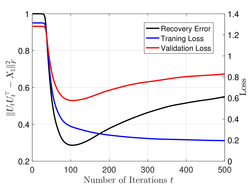
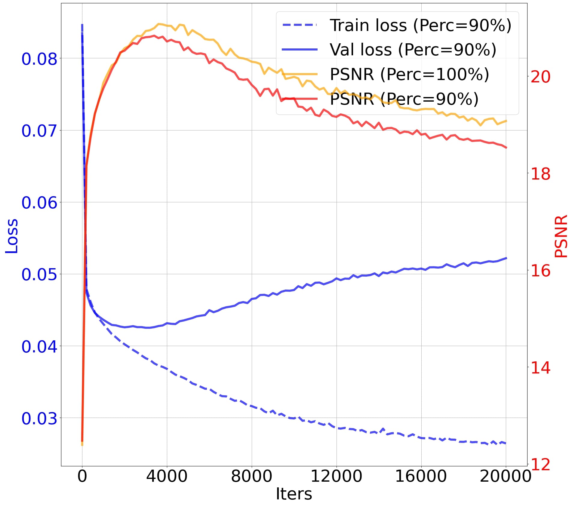
On the other hand, in the noiseless case, the work [22, 23, 24] replace $U\in\mathbb{R}^{n\times r}$ in (2) by a square matrix $U\in\mathbb{R}^{n\times n}$, for which the rank information $r_{\natural}$ is no longer required. With a very small random initialization, gradient descent is guaranteed to find the ground-truth matrix $X_{\natural}$, even when $r=n$ and $\mathcal{A}$ only satisfies $2r_{\natural}$-RIP. This is in sharp contrast to the works [19, 20] that require $2r$-RIP, which in general is not satisfied when $r=n$ since it will require full measurements of a matrix. The principal idea behind [22, 23, 24] is that even though there exist infinite number of solutions $U$ such that $\mathcal{A}(UU^{\top})=y=\mathcal{A}(X_{\natural})$, gradient descent with small initialization produces an implicit bias that towards low-rank solutions. Nevertheless, such a conclusion cannot be directly applied to the noisy case since a square matrix $U$ can overfit the noise and does not produce the desired solution $X_{\natural}$. As shown in Figure 1, while the training loss (blue curve) keeps decreasing, the iterates $U_{t}$ eventually tend to overfit as indicated by the recovery error (black curve).

Table 1: Comparison with prior theory for over-parameterized noisy matrix sensing (2). Here $\widehat{X}$ denotes the recovered matrix, $\sigma^{2}$ is the variance proxy for the additive noise.

	RIP requirement	Initialization	Statistical error $\|\widehat{X}-X_{\natural}\|_{\tiny\mathrm{F}}^{2}$
[19, 20] ($r_{\natural}\leq r\leq\tilde{\mathcal{O}}(m/n)$)	$2r$-RIP	Good initialization: $U_{0}U_{0}^{\top}$ close to $X_{\natural}$	$\tilde{\mathcal{O}}(\sigma^{2}nr/m)$
Ours ($r\geq r_{\natural}$)	$2r_{\natural}$-RIP	Random small initialization	$\tilde{\mathcal{O}}(\sigma^{2}nr_{\natural}/m)$

Overview of our methods and contributions

In this paper, we address the above challenges in the over-parameterized noisy matrix recovery problem (2) by analyzing the trajectory of gradient descent iterations. In particular, we extend the analysis in [24] to noisy measurements and show that gradient descent with small initialization generates iterations toward the ground-truth matrix and achieves nearly information-theoretically optimal recovery within $\tilde{\mathcal{O}}(1)$ steps. This is summarized in the following informal theorem.

Theorem 1.1 (Informal).

Assume $\mathcal{A}$ satisfies $2r_{\natural}$-RIP. With small random initialization and any $r\geq r_{\natural}$, gradient descent efficiently produces an estimator with a statistical error of $\tilde{\mathcal{O}}(\sigma^{2}nr_{\natural}/m)$ within $\tilde{\mathcal{O}}(1)$ steps.

As summarized in Table 1, our work improves upon [19, 20] by showing that gradient descent can achieve minimax optimal statistical error $\tilde{\mathcal{O}}(\sigma^{2}nr_{\natural}/m)$ with only $2r_{\natural}$-RIP requirement on $\mathcal{A}$, even in the extreme over-parameterized case $r=n$. Moreover, vanilla gradient descent only converges at a sublinear rate in [19], which is improved to a linear converge rate by a preconditioned gradient descent [20]. Our work shows that vanilla gradient descent with small random initialization rather than a good initialization actually finds a statistical optimal recovery within $\tilde{\mathcal{O}}(1)$ steps. On the other hand, since we only require $\mathcal{A}$ satisfies $2r_{\natural}$-RIP, our result requires gradient descent to stop appropriately. Towards that goal, we propose a practical and efficient early stopping strategy based on the common hold-out method. In particular, we remove a subset from the measurements, denoted by $y_{\textup{val}}$ with the corresponding sensing operator $\mathcal{A}_{\textup{val}}$. We then use the validation loss $\frac{1}{2}\left\|\mathcal{A}_{\textup{val}}\left(U_{t}U_{t}^{\top}\right)-y_{\textup{val}}\right\|_{2}^{2}$ to monitor the recovery error $\frac{1}{2}\|U_{t}U_{t}^{\top}-X_{\natural}\|_{\tiny\mathrm{F}}^{2}$ (see red and black curves in Figure 1) and detect the valley of the recovery error curve.

Theorem 1.2 (Informal).

The validation approach identifies an iterate with a statistical error of $\tilde{\mathcal{O}}(\sigma^{2}nr_{\natural}/m)$, which is minimax optimal.

This result shows that the gap (in terms of recovery error) between our detected iterate and the best iterate is typically very small, which is further verified by Figure 1 and experiments in Section 4.

Other related work

Over-parameterized matrix recovery has also been studied in the presence of sparse additive noise [25, 26, 27, 28], which either models the noise as an explicit term in the optimization objective [25], or uses subgradient methods with diminishing step sizes for the $\ell_{1}$ loss of [26, 27, 28]. Though the work [28] also extends the approach of $\ell_{1}$ loss to the Gaussian noise, it is based on the assumption of the so-called sign-RIP for the sensing operator. Such property is only known to be satisfied by Gaussian distribution and the proof relies heavily on the rotation invariance of Gaussian. This sign-RIP condition is unknown and potentially not to hold for other distributions, such as the Rademacher distribution. Also, subgradient method requires diminishing step sizes which need to be fine-tuned in practice.

Extension to image recovery with a deep image prior (DIP)

Learning over-parameterized models is becoming an increasingly important area in machine learning. Beyond low-rank matrix recovery problem, over-parameterized model has also been formally studied for several other fundamental problems, including compressive sensing [29, 30] (which also uses a similar validation approach), logistic regression on linearly separated data [31], nonlinear least squares [32], deep linear neural networks and matrix factorization [33, 34, 35, 36], deep image prior [37, 38] and so on. Among these, closely related to the matrix recovery problem is the deep image prior (DIP) which over-parameterizes an image by a deep network, a non-linear multi-layer extension of the factorization $UU^{\top}$. While DIP has shown impressive results on image recovery tasks, it requires appropriate early stopping to avoid overfitting. The work [38, 39] propose an early stopping strategy by either training a coupled autoencoder or tracking the trend of the variance of the iterates, which are more complicated than the validation approach. In Section 4, we demonstrate by experiments that the proposed validation approach, partitioning the image pixels into a training set and a validation set, can be used to identify appropriate stopping for DIP efficiently. The novelty lies in partitioning the image pixels, which are traditionally considered one giant piece for training.

Notation

For a subspace $L\subset^{n}$, we use $V_{L}$ to denote an orthonormal representation of the subspace space of $L$, i.e., $V_{L}$ has $\dim(L)$ orthonormal columns and the columns span $L$. Moreover, we denote a representation of the orthogonal space of $L$ by $V_{L^{\perp}}$. We use the same notations $V_{L}$ and $V_{L^{\perp}}$ representing the column space of a matrix $L$ and its orthogonal complement respectively. We denote the singular values of a matrix $X\in^{n\times n}$ by $\sigma_{1}(X)\geq\dots\geq\sigma_{n}(X)$. The condition number of $X_{\natural}$ is denoted as $\kappa=\frac{\sigma_{1}(X_{\natural})}{\sigma_{r_{\natural}}(X_{\natural})}$. For two quantities $a,b\in$, the inequalities $a\gtrsim b$ and $b\lesssim a$ means $b\leq ca$ for some universal constant $c$. A random variable $Z$ with mean $\mu$ is subgaussian with variance proxy $\sigma$, denoted as $Z\sim\text{subG}(\sigma)$, if $\mathbb{E}(\exp(\lambda(Z-\mu)))\leq\exp(\sigma^{2}\lambda^{2}/2)$ for any $\lambda\in$.

2 Algorithm and Analysis

In this section, we first present gradient descent for Problem (2) and a few preliminaries. In Section 2.2, we give the main result that gradient descent coupled with small random initialization produces an iterate achieving optimal statistical error. Finally, we conclude this section with the proof strategy of our main result.

2.1 Algorithm and preliminaries

Gradient descent proceeds as follows: pick a stepsize $\eta>0$, an initialization direction $U\in^{n\times r}$ and a size $\alpha$, initialize

$$U_{0}=\alpha U,\quad\text{and iterate}\quad U_{t+1}=U_{t}-\eta\cdot\underbrace{\frac{1}{m}\cdot\left(\mathcal{A}^{*}(\mathcal{A}(U_{t}U_{t}^{\top}-X_{\natural}))-\mathcal{A}^{*}(e)\right)U_{t}}_{\nabla f(U_{t})}.$$ (3)

Here $\mathcal{A}^{*}$ is the adjoint operator of $\mathcal{A}$. We equip the space ^m with the dot product, and the space ^n×n with the standard trace product. The corresponding norms are the $\ell_{2}$ norm $\left\|\cdot\right\|_{2}$ and $\|\cdot\|_{F}$ respectively.

To analyze the behavior of the gradient descent method (3), we consider the following restricted isometry condition [1], which states that the map $\mathcal{A}$ approximately preserves the $\ell_{2}$ norm between its input and output spaces.

Definition 2.1.

[$(k,\delta)$-RIP] A linear map $\mathcal{A}:\mathbb{R}^{n\times n}\rightarrow\mathbb{R}^{m}$ satisfies $(k,\delta)$ restricted isometry property (RIP) for some integer $k>0$ and $\delta\in[0,1]$ if for any matrix $X\in^{n\times n}$ with $\operatorname{rank}(X)\leq k$, the following inequalities hold:

$$(1-\delta)\|X\|_{F}^{2}\leq\frac{\left\|\mathcal{A}(X)\right\|_{2}^{2}}{m}\leq(1+\delta)\|X\|_{F}^{2}.$$ (4)

Let $\mathcal{A}(Z)=(\langle A_{1},Z\rangle,\dots,\langle A_{m},Z\rangle)^{\top}$ for any $Z\in^{n\times n}$. According to [2, Thereom 2.3], the $(k,\delta)$-RIP condition is satisfied with high probability if each sensing matrix $A_{i}$ contains iid subgaussian entries so long as $m\gtrsim\frac{nk\log(1/\delta)}{\delta^{2}}$.

Thus, if a linear map $\mathcal{A}$ satisfies RIP, then $\frac{1}{m}\left\|\mathcal{A}(X)\right\|_{2}^{2}$ is approximately $\|X\|_{F}^{2}$ for low rank $X$. Interestingly, the nearness in the function value actually implies the nearness in the gradient under certain norms as the following proposition states.

Proposition 2.2.

[24, Lemma 7.3] Suppose $\mathcal{A}$ satisfies $(k,\delta)$-RIP. Then for any matrix $X\in^{n\times n}$ with rank no more than $k$, and any matrix $Z\in^{n\times n}$ we have the following two inequalities:

$$\|(\mathcal{I}-\frac{\mathcal{A}^{*}\mathcal{A}}{m})(X)\|\leq\delta\|X\|_{F},$$ (5)

$$\|(\mathcal{I}-\frac{\mathcal{A}^{*}\mathcal{A}}{m})(Z)\|\leq\delta\|Z\|_{\ast}.$$ (6)

Here $\|\cdot\|$ and $\|\cdot\|_{\ast}$ denote the spectral norm and nuclear norm, respectively, and $\mathcal{I}$ denotes the identity map.

To see the usefulness of the above bound, letting $\mathcal{D}=\mathcal{I}-\frac{\mathcal{A}^{*}\mathcal{A}}{m}$, we may decompose (3) as the following:

$$U_{t+1}=U_{t}-\eta(U_{t}U_{t}^{\top}-X_{\natural})U_{t}+\eta[\mathcal{D}(U_{t}U_{t}^{\top}-X_{\natural})]U_{t}.$$ (7)

Thus we may regard $[\mathcal{D}(U_{t}U_{t}^{\top}-X_{\natural})]U_{t}$ as a perturbation term and focus on analyzing $U_{t+1}=U_{t}-\eta(U_{t}U_{t}^{\top}-X_{\natural})U_{t}$. Proposition 2.2 is then useful in controlling this perturbation. Specifically, the first inequality, which we call spectral-to-Frobenius bound, is useful in ensuring some subspaces alignment and a certain signal term indeed increasing at a fast speed, while the second one, which we call spectral-to-nuclear bound, ensures that we can deal with matrices with rank beyond $2r_{\natural}$. See Section A.1 for a more detailed explanation.

2.2 Optimal statistical error guarantee

We now give a rigorous statement showing that some gradient descent iterates $U_{t}$ indeed achieve optimal statistical error.

Theorem 2.3.

We assume that $\mathcal{A}$ satisfies $(2r_{\natural},\delta)$-RIP with $\delta\leq c\kappa^{-2}r_{\natural}^{-1/2}$. Suppose the noise vector $e$ has independent mean-zero SubG($\sigma^{2}$) entries and $m\gtrsim\kappa^{2}n\frac{\sigma^{2}}{\sigma_{r_{\natural}}^{2}(X_{\natural})}$. Further suppose the stepsize $\mu\leq c\kappa^{-2}\|X_{\natural}\|^{-1}$ and $r\geq r_{\natural}$. If the scale of initialization satisfies

$$\alpha\lesssim\min\left\{\frac{1}{\kappa^{4}n^{4}}\left(C\kappa n^{2}\right)^{-6\kappa}\sqrt{\|X_{\natural}\|},\;\kappa\sqrt{\frac{nr_{\natural}}{m\|X_{\natural}\|}}\sigma\right\}.$$

then after $\hat{t}\lesssim\frac{1}{\mu\sigma_{\min}(X_{\natural})}\log\left(\frac{Cn\kappa\sqrt{\|X_{\natural}\|}}{\alpha}\right)$ iterations, we have

$$\|U_{\hat{t}}U_{\hat{t}}^{\top}-X_{\natural}\|_{\tiny\mathrm{F}}^{2}\lesssim\sigma^{2}\kappa^{2}\frac{r_{\natural}n}{m}.$$

with probability at least $1-\tilde{C}/n-\tilde{C}\exp(-\tilde{c}r)$, here $C,\tilde{C},c,\tilde{c}>0$ are fixed numerical constants.

We note that unlike those bounds obtained in [19, 20], our final error bound $\mathcal{O}(\kappa^{2}\sigma^{2}\frac{nr_{\natural}}{m})$ has no extra logarithmic dependence on the dimension $n$ or the over-specified rank $r$. The initialization size $\alpha$ needs to be dimensionally small, which we think is mainly an artifact of the proof. In our experiments, we set $\alpha=10^{-6}$. We explain the rationale behind this small random initialization in Section A.1.

The requirement that $\delta$ needs to be smaller than $\frac{1}{\sqrt{r}}$ is a long-standing technical question in the field [8, 24] and we did not attempt to resolve this issue. However, we do note that the main reason for this dependence is from the early stage of the algorithms. For those algorithms with a strategy of “initialization+local refinement” [8, 5], the guarantee of initialization itself requires that $\delta<\frac{1}{\sqrt{r}}$. For those algorithms with small (random) initialization [23, 24], such requirement comes from the analysis of the initial few iterations.

To prove Theorem 2.3, we utilize the following theorem which only requires a deterministic condition on the noise matrix $\mathcal{A}^{*}(e)$, and allows a larger range of the choice of $\alpha$. Its detailed proof can be found in Appendix A and follows a similar strategy as [24] with technical adjustments due to the noise matrix $\mathcal{A}^{*}(e)$.

Theorem 2.4.

Instate the same assumption in Theorem 2.3 for $\mathcal{A}$, the stepsize $\mu$ and the rank parameter $r$. Let $E=\frac{1}{m}\mathcal{A}^{*}(e)$ and assume $\|E\|\leq c\kappa^{-1}\sigma_{\min}(X_{\natural}).$ If the scale of initialization satisfies

$$\alpha\lesssim\frac{1}{\kappa^{4}n^{4}}\left(C\kappa n^{2}\right)^{-6\kappa}\sqrt{\|X_{\natural}\|},$$

then after $\hat{t}\lesssim\frac{1}{\mu\sigma_{\min}(X_{\natural})}\log\left(\frac{Cn\kappa\sqrt{\|X_{\natural}\|}}{\alpha}\right)$ iterations, we have

$$\frac{\|U_{\hat{t}}U_{\hat{t}}^{\top}-X_{\natural}\|_{\tiny\mathrm{F}}}{\|X_{\natural}\|}\lesssim\frac{\alpha}{\sqrt{\|X_{\natural}\|}}+\sqrt{r_{\natural}}\kappa\frac{\|E\|}{\|X_{\natural}\|}$$

with probability at least $1-\tilde{C}/n-\tilde{C}\exp(-\tilde{c}r)$, here $C,\tilde{C},c,\tilde{c}>0$ are fixed numerical constants.

Let us now prove Theorem 2.3.

Proof of Theorem 2.3.

Consider the following bound on $\|\mathcal{A}^{*}(e)\|$,

$$\frac{1}{m}\|\mathcal{A}^{*}(e)\|\lesssim\sqrt{\frac{n}{m}}\sigma\leq c\kappa^{-1}\sigma_{r_{\natural}}(X_{\natural}).$$ (8)

The first inequality comes from standard random matrix theory [21, Lemma 1.1] and the second is due to our assumption on $m$. Now Theorem 2.3 simply follows from Theorem 2.4 by plugging in the above bound and the choice of $\alpha$. ∎

In Theorem 2.3, we only know some iterate $U_{\hat{t}}$ will achieve the optimal statistical error, and the question of how to pick such iterate remains. We detail the procedure in Section 3.

3 Early Stopping

In this section, we propose an efficient method for early stopping, i.e., finding the best iterate $X_{t}=U_{t}U_{t}^{\top}$ that has the smallest recovery error $\left\|X_{t}-X_{\natural}\right\|_{F}$. We exploit the validation approach, a common technique used in machine learning. Specifically, we remove a subset from the measurements, denoted by $y_{\textup{val}}$ with the corresponding sensing operator $\mathcal{A}_{\textup{val}}$ and noise vector $e_{\textup{val}}$. The remaining data samples form the training dataset, and we denote it as $(y_{\text{train}},\mathcal{A}_{\text{train}})$. More precisely, the data $(y,\mathcal{A})$ can be explicitly expressed as $\{(y_{i},A_{i})\}_{i=1}^{m}$ where each data sample $(y_{i},A_{i})\in^{1+n\times n}$. We split the data into $m_{\text{train}}$ training samples with index set $\mathcal{I}_{\text{train}}$, and the rest $m_{\textup{val}}$ samples is for the validation purpose with index set $\mathcal{I}_{\textup{val}}$. The validation subset is not used for training, but rather for measuring the recovery error $\left\|X_{t}-X_{\natural}\right\|_{F}$.

Lemma 3.1.

Suppose each entry in $A_{i}$, $i\in\mathcal{I}_{\textup{val}}$ is i.i.d. $\textup{subG}(c_{1})$ with mean zero and variance $1$ and each $e_{i}$ is also a zero-mean sub-Gaussian distribution $\textup{subG}(c_{2}\sigma^{2})$ with variance $\sigma^{2}$, where $c_{1},c_{2}\geq 1$ are absolute constants. Also assume $D_{1},\ldots,D_{T}$ are independent of $\mathcal{A}_{\textup{val}}$ and $e_{\textup{val}}$. Then for any $\delta_{\textup{val}}>0$, given $m_{\textup{val}}\geq C_{1}\frac{\log T}{\delta_{\textup{val}}^{2}}$, with probability at least $1-2T\exp\left(-C_{2}m_{\textup{val}}\delta_{\textup{val}}^{2}\right)$,

$$\left|\left\|\mathcal{A}_{\textup{val}}(D_{t})+e\right\|_{F}^{2}-m_{\textup{val}}(\left\|D_{t}\right\|_{F}^{2}+\sigma^{2})\right|\leq\delta_{\textup{val}}m_{\textup{val}}(\left\|D_{t}\right\|_{F}^{2}+\sigma^{2}),\forall\ t=1,\ldots,T,$$

where $C_{1},C_{2}\geq 0$ are constants that may depend on $c_{1}$ and $c_{2}$.

Proof of Lemma 3.1.

For any $D\in\mathbb{R}^{n\times n}$, $\left\langle A_{i},D\right\rangle+e_{i}$ is a zero-mean sub-Gaussian random variable with variance $\|D\|_{\tiny\mathrm{F}}^{2}+\sigma^{2}$ and sub-Gaussian norm

$$\left\|\left\langle A_{i},D\right\rangle+e_{i}\right\|_{\psi_{2}}^{2}\leq C\left(c_{1}\|D\|_{\tiny\mathrm{F}}^{2}+c_{2}\sigma^{2}\right)\leq C_{1}\left({\|D\|_{\tiny\mathrm{F}}^{2}}+\sigma^{2}\right),$$

where $C$ is an absolute constant and $C_{1}\geq 0$ is a constant depending on $c_{1}$ and $c_{2}$. This implies that $(\left\langle A_{i},D\right\rangle+e_{i})^{2}$ is a sub-exponential random variable with sub-exponential norm the same as $\left\|\left\langle A_{i},D\right\rangle+e_{i}\right\|_{\psi_{2}}^{2}$ [40, Theorem 2.7.6]. Thus, for any $t\geq 0$, we have [40, Theorem 2.8.1]

$$\mathbb{P}\left[\left|\left\|\mathcal{A}_{\textup{val}}(D)+e\right\|_{F}^{2}-m_{\textup{val}}(\left\|D\right\|_{F}^{2}+m_{\textup{val}}\sigma^{2})\right|\geq tm_{\textup{val}}C_{1}(\left\|D\right\|_{F}^{2}+\sigma^{2})\right]$$

$$\leq 2\exp\left(-C_{2}\min\left(m_{\textup{val}}t^{2},m_{\textup{val}}t\right)\right),$$

where $C_{2}>0$ is an absolute constant. Taking $t=\delta_{\textup{val}}/C_{1}$ and $m_{\textup{val}}=O(\frac{\log^{2}T}{\delta_{\textup{val}}^{2}})$, we have

$$\mathbb{P}\left[\cup_{t=1}^{T}\left\{\left|\left\|\mathcal{A}_{\textup{val}}(D_{t})+e\right\|_{F}^{2}-m_{\textup{val}}(\left\|D_{t}\right\|_{F}^{2}+\sigma^{2})\right|\geq\delta_{\textup{val}}m_{\textup{val}}(\left\|D_{t}\right\|_{F}^{2}+\sigma^{2})\right\}\right]$$

$$\leq 2T\exp\left(-C_{2}m_{\textup{val}}\delta_{\textup{val}}^{2}\right),$$

where we absorb $C_{1}$ into $C_{2}$ in the last equation. ∎

With Lemma 3.1, the following result establishes guarantees for the validation approach.

Lemma 3.2.

Let $\widehat{t}=\operatorname*{\text{arg~{}min}}_{1\leq t\leq T}\left\|\mathcal{A}_{\textup{val}}(D_{t})+e\right\|_{2}$ and $\widetilde{t}=\operatorname*{\text{arg~{}min}}_{1\leq t\leq T}\|D_{t}\|_{\tiny\mathrm{F}}$. Assume

$$(1-\delta_{\textup{val}})(\left\|D_{t}\right\|_{F}^{2}+\sigma^{2})\leq\frac{1}{m_{\textup{val}}}\left\|\mathcal{A}_{\textup{val}}(D_{t})+e\right\|_{F}^{2}\leq(1+\delta_{\textup{val}})(\left\|D_{t}\right\|_{F}^{2}+\sigma^{2}),\ \forall t=1,\ldots,T.$$

Then,

$$\|D_{\widehat{t}}\|_{\tiny\mathrm{F}}^{2}\leq\frac{1+\delta_{\textup{val}}}{1-\delta_{\textup{val}}}\|D_{\widetilde{t}}\|_{\tiny\mathrm{F}}^{2}+\frac{2\delta_{\textup{val}}}{1-\delta_{\textup{val}}}\sigma^{2}$$

Proof.

Since $\widehat{t}=\operatorname*{\text{arg~{}min}}_{1\leq t\leq T}\left\|\mathcal{A}(D_{t})+e\right\|_{2}$, we have

$$\|D_{\widehat{t}}\|_{\tiny\mathrm{F}}^{2}+\sigma^{2} \leq\frac{1}{1-\delta_{\textup{val}}}\left\|\mathcal{A}_{\textup{val}}(D_{\widehat{t}})+e\right\|_{F}^{2}\leq\frac{1}{1-\delta_{\textup{val}}}\left\|\mathcal{A}_{\textup{val}}(D_{\widetilde{t}})+e\right\|_{F}^{2}\leq\frac{1+\delta_{\textup{val}}}{1-\delta_{\textup{val}}}(\left\|D_{\widetilde{t}}\right\|_{F}^{2}+\sigma^{2}),$$

which further implies that

$$\|D_{\widehat{t}}\|_{\tiny\mathrm{F}}^{2}\leq\frac{1+\delta_{\textup{val}}}{1-\delta_{\textup{val}}}\|D_{\widetilde{t}}\|_{\tiny\mathrm{F}}^{2}+\frac{2\delta_{\textup{val}}}{1-\delta_{\textup{val}}}\sigma^{2}.$$

∎

Now lett $\delta_{\textup{val}}=\frac{\kappa^{2}nr_{\natural}}{m_{\text{train}}}$ and $D_{t}=U_{t}U_{t}^{\top}-X_{\natural}$ where $U_{t},t=1,\dots,T$ are iterates from (3) with $(y,\mathcal{A})$ replaced by $(y_{\text{ train}},\mathcal{A}_{\text{train}})$. With this choice of $\delta_{\text{val}}$ and $D_{t}$, and combining the above lemmas, we reach the main theorem of this section.

Theorem 3.3.

Fix $\epsilon\in(0,1)$. Under the same assumption as Theorem 2.3 with $(y,\mathcal{A})$ replaced by $(y_{\text{train}},\mathcal{A}_{\text{train}})$, and the same assumption of Lemma 3.2, further suppose $\frac{(nr_{\natural})^{2}\kappa^{2}m_{\textup{val}}}{m^{2}_{\text{train}}}\geq C\frac{\log T}{\log(\frac{1}{\epsilon})}$ and $T>C\kappa^{4}\log(n+r)$ for some universal $C>0$. Also let $\widehat{t}=\operatorname*{\text{arg~{}min}}_{1\leq t\leq T}\left\|\mathcal{A}_{\textup{val}}(D_{t})+e\right\|_{2}$. Then with probability at least $1-\epsilon$, we have

$$\|U_{\widehat{t}}U_{\widehat{t}}^{\top}-X_{\natural}\|_{F}^{2}\leq C\frac{\kappa^{2}\sigma^{2}r_{\natural}n}{m_{\text{train}}}.$$ (9)

We note the condition $\frac{(nr_{\natural})^{2}\kappa^{2}m_{\textup{val}}}{m^{2}_{\text{train}}}\geq C\frac{\log T}{\log(\frac{1}{\epsilon})}$ is satisfied when $m_{\textup{val}}$ and $m_{\text{train}}$ are on the same order and not quadratic in $n$ and the running time $T$ is not exponential in the dimension and condition number.

4 Experiments

In this section, we conduct a set of experiments on matrix sensing and matrix completion to demonstrate the performance of gradient descent with validation approach for over-parameterized matrix recovery. We also conduct experiments on image recovery with deep image prior to show potential applications of the validation approach for other related unsupervised learning problems.

4.1 Matrix sensing

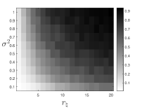
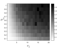
In these experiments, we generate a rank-$r_{\natural}$ matrix $X_{\natural}\in\mathbb{R}^{n\times n}$ by setting $X_{\natural}=U_{\natural}U_{\natural}^{\top}$ with each entries of $U_{\natural}\in\mathbb{R}^{n\times r_{\natural}}$ being normally distributed random variables, and then normalize $X_{\natural}$ such that $\|X_{\natural}\|_{\tiny\mathrm{F}}=1$. We then obtain $m$ measurements $y_{i}=\langle A_{i},X_{\natural}\rangle+e_{i}$ for $i=1,\ldots m$, where entries of $A_{i}$ are i.i.d. generated from standard normal distribution, and $e_{i}$ is a Gaussian random variable with zero mean and variance $\sigma^{2}$. We set $n=50,m=1000$, and vary the rank $r_{\natural}$ from 1 to 20 and the noise variance $\sigma^{2}$ from 0.1 to 1. We then split the $m$ measurements into $m_{\textup{train}}=900$ training data and $m_{\textup{val}}=100$ validation data to get the training dataset $(y_{\text{train}},\mathcal{A}_{\text{train}})$ and validation dataset $(y_{\textup{val}},\mathcal{A}_{\textup{val}})$, respectively. To recover $X_{\natural}$, we use a square factor $U\in\mathbb{R}^{n\times n}$ and then solve the over-parameterized model (2) on the training data $(y_{\text{train}},\mathcal{A}_{\text{train}})$ using gradient descent with step size $\eta=0.5$, $T=500$ iterations, and initialization $U_{0}$ of Gaussian distributed random variables with zero mean and variance $\alpha^{2}$; we set $\alpha=10^{-6}$. Within all the generated iterates $U_{t}$, we select

$$\begin{split}\widetilde{t}=\operatorname*{\text{arg~{}min}}_{1\leq t\leq T}\|U_{t}U_{t}^{\top}-X_{\natural}\|_{\tiny\mathrm{F}},\quad\widehat{t}&=\operatorname*{\text{arg~{}min}}_{1\leq t\leq T}\left\|\mathcal{A}_{\textup{val}}\left(U_{t}U_{t}^{\top}\right)-y_{\textup{val}}\right\|_{2}.\end{split}$$ (10)

That is, $U_{\widetilde{t}}$ is the best iterate to represent the ground-truth matrix $X_{\natural}$, while $U_{\widehat{t}}$ is the one selected based on the validation loss.

For each pair of $r_{\natural}$ and $\sigma^{2}$, we conduct 10 Monte Carlo trails and compute the average of the recovered errors for $\|U_{\widetilde{t}}U_{\widetilde{t}}^{\top}-X_{\natural}\|_{\tiny\mathrm{F}}^{2}$ and $\|U_{\widehat{t}}U_{\widehat{t}}^{\top}-X_{\natural}\|_{\tiny\mathrm{F}}^{2}$. The results are shown in Figure 2 (a) and (b). In both plots, we observe that the recovery error is proportional to $r_{\natural}$ and $\sigma^{2}$, in consistent with Theorem 2.3 and Equation 9. Moreover, comparing Figure 2 (a) and (b), we observe similar recovery error for both $U_{\widetilde{t}}$ and $U_{\widehat{t}}$, demonstrating the performance of the validation approach.

(a) $\|U_{\widetilde{t}}U_{\widetilde{t}}^{\top}-X_{\natural}\|_{\tiny\mathrm{F}}^{2}$

(b) $\|U_{\widehat{t}}U_{\widehat{t}}^{\top}-X_{\natural}\|_{\tiny\mathrm{F}}^{2}$

(c) $\|U_{\widetilde{t}}U_{\widetilde{t}}^{\top}-X_{\natural}\|_{\tiny\mathrm{F}}^{2}$

(d) $\|U_{\widehat{t}}U_{\widehat{t}}^{\top}-X_{\natural}\|_{\tiny\mathrm{F}}^{2}$

Figure 2: Recover error (whiter indicates better recovery) of gradient descent for solving over-parameterized noisy $(a,b)$ matrix sensing problem measured by $(a)$ the best iterate $U_{\widetilde{t}}$ and $(b)$ the iterate $U_{\widehat{t}}$ selected via validation approach, and $(c,d)$ matrix completion measured by $(c)$ $U_{\widetilde{t}}$ and $(d)$ $U_{\widehat{t}}$. $\widetilde{t}$ and $\widehat{t}$ are formally defined in (10).

4.2 Matrix completion

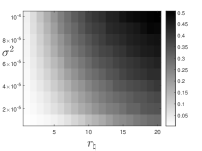
In the second set of experiments, we test the performance on matrix completion where we want to recover a low-rank matrix from incomplete measurements. Similar to the setup for matrix sensing, we generate a rank-$r_{\natural}$ matrix $X_{\natural}$ and then randomly obtain $m$ entries with additive Gaussian noise of zero mean and variance $\sigma^{2}$. In this case, each selected entry can be viewed as obtained by a sensing matrix that contains zero entries except for the location of the selected entry being one. Thus, we can apply the same gradient descent to solve the over-parameterized problem to recovery the ground-truth matrix $X_{\natural}$. In these experiments, we set $n=50,m=1000,\eta=0.5,T=500,\alpha=10^{-3}$, and vary the rank $r_{\natural}$ from 1 to 20 and the noise variance $\sigma^{2}$ from $10^{-5}$ to $10^{-4}$. We display the recovered error in Figure 2 (c) and (d). Similar to the results in matrix sensing, we also observe from Figure 2 (c) and (d) that gradient descent with validation approach produces a good solution for solving over-parameterized noisy matrix completion problem.

4.3 Deep image prior

(a)

(b)

(c)

(d)

(e)

(f)

(g)

(h)

Figure 3: Image denoising by DIP. From left to right: the noisy image, the image with the smallest validation loss, the image with the best PSNR, and the learning curves in terms of training loss, validation loss, PSNR. Here, the top row is for Gaussian noise with mean 0 and variance 0.1, while bottom row is for salt and pepper noise where $10$ percent of pixels are randomly corrupted. In (d) and (h), Perc = 90% means we train UNet on 90% of pixels and the rest of 10% pixels are used for validation; Perc = 100% means we train the network with the entire pixels. The model is optimized with Adam for 5000 iterations. The numbers listed in the captions show the corresponding PSNR.

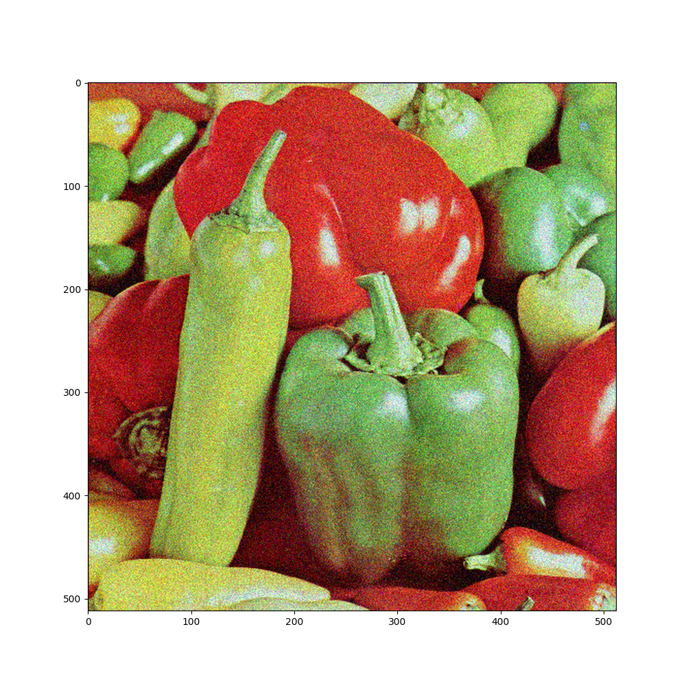
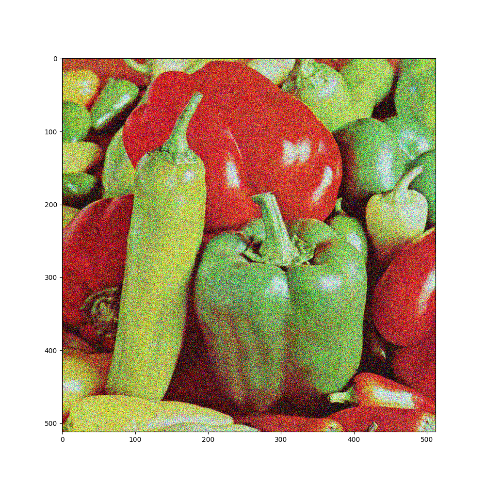
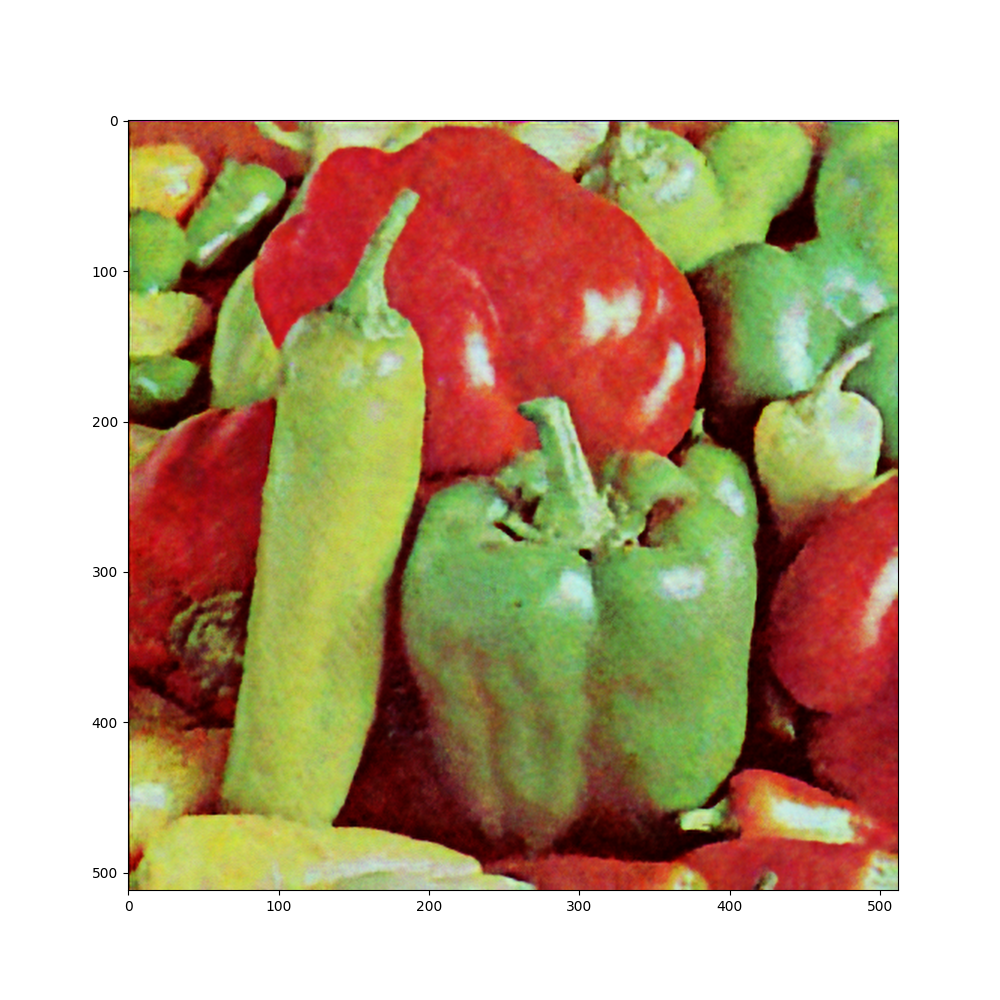
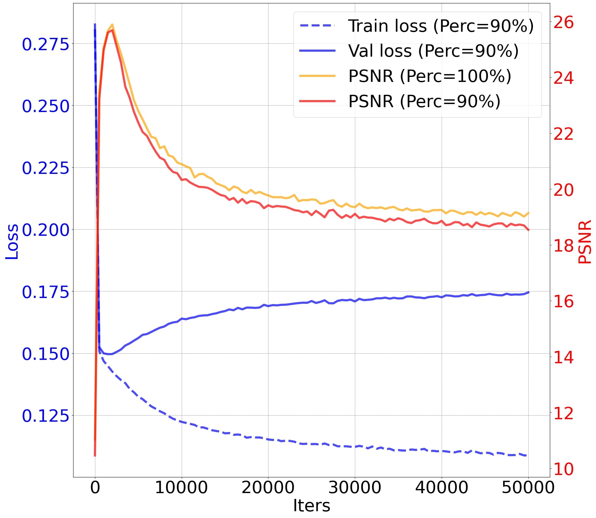
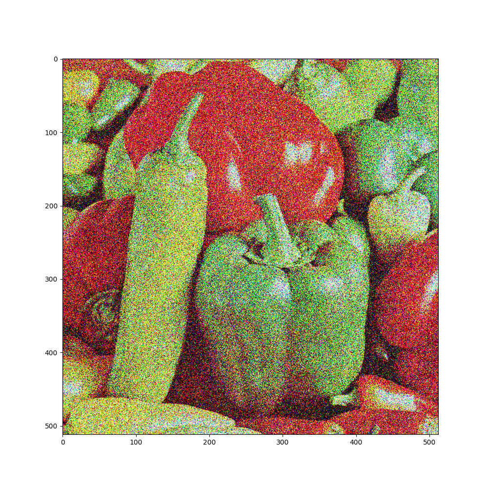
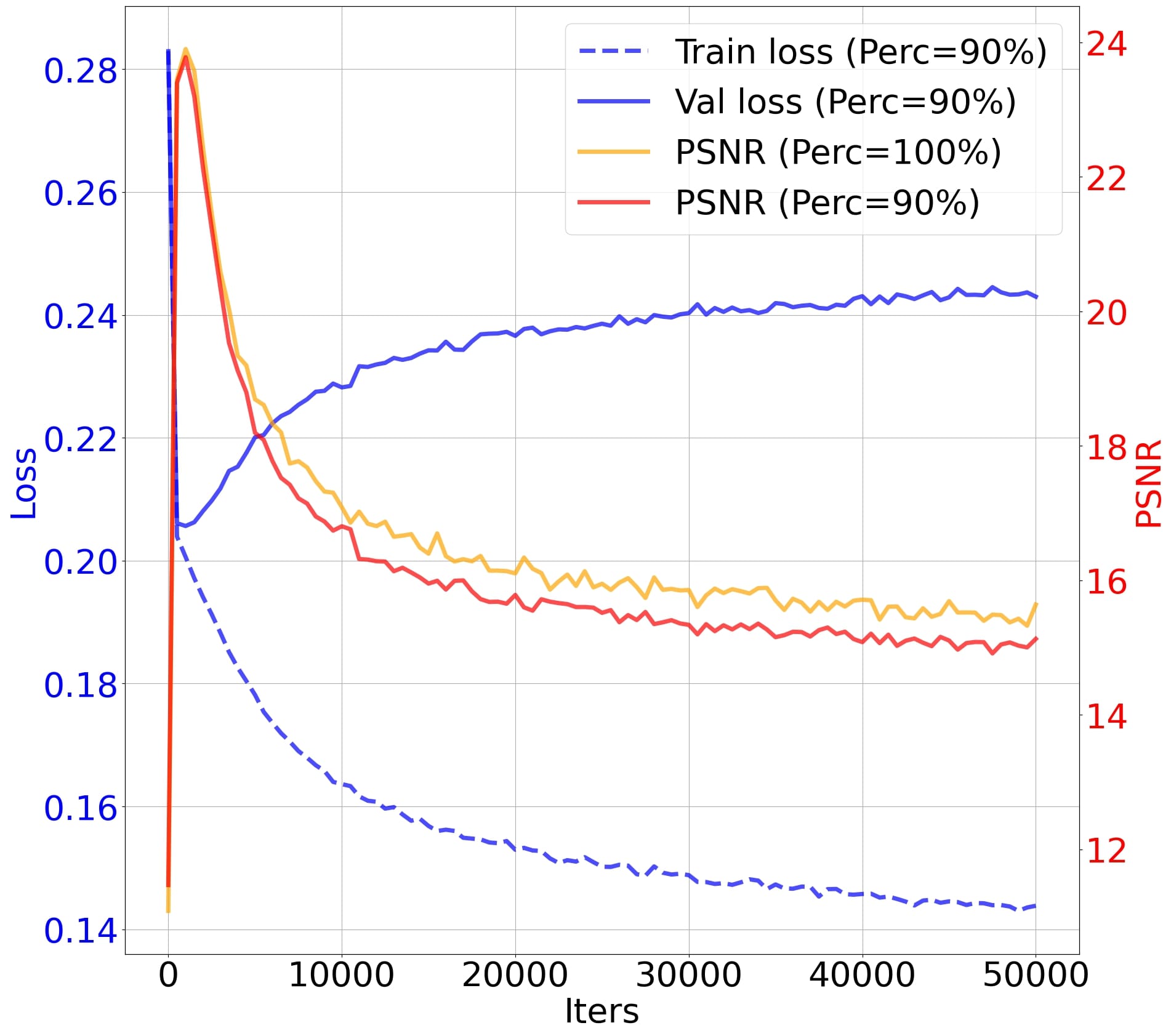
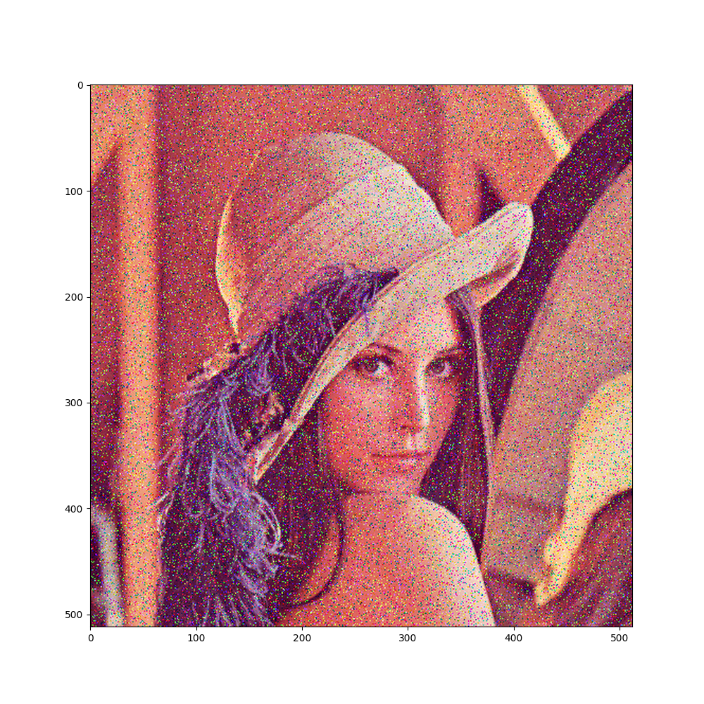
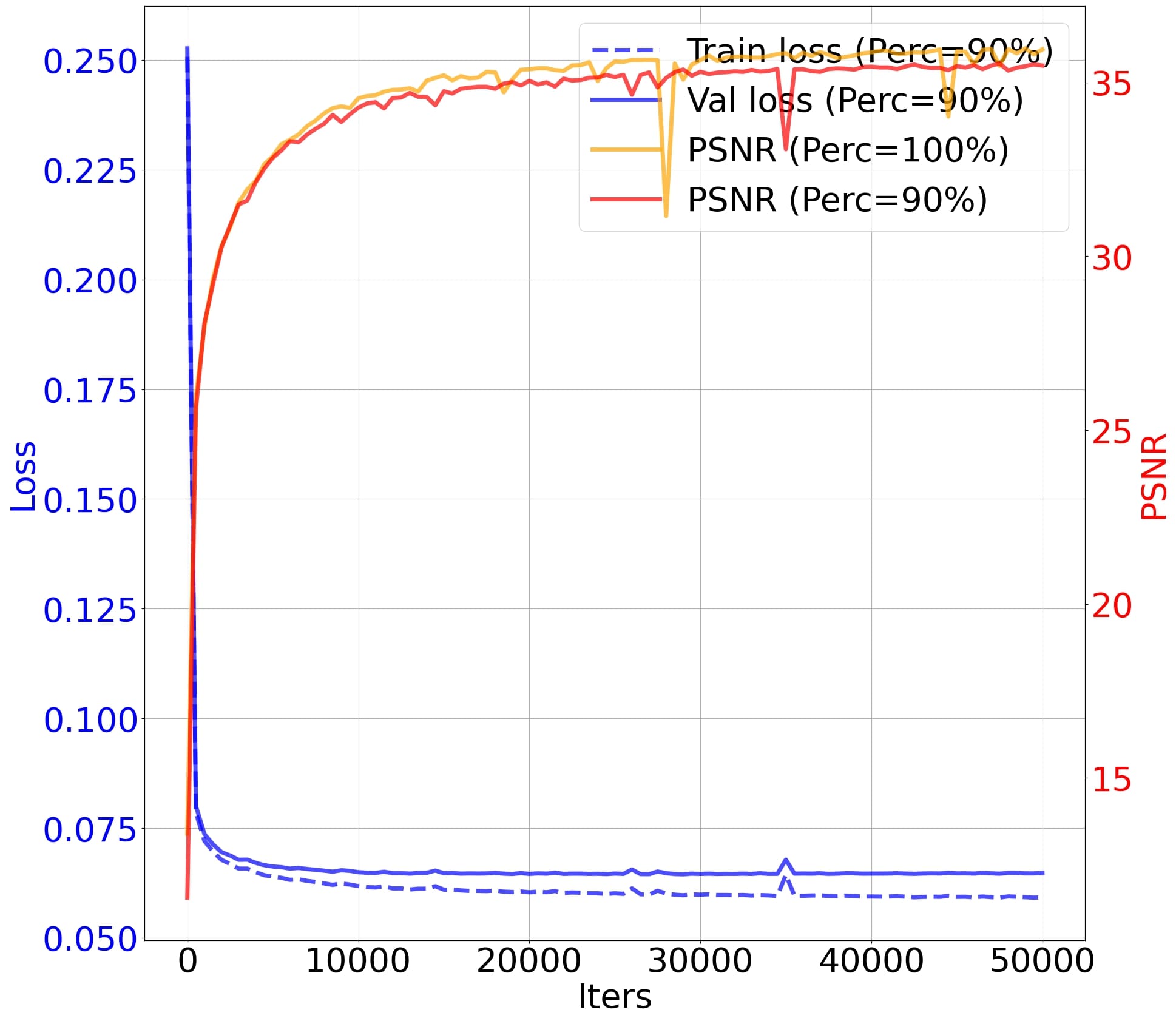
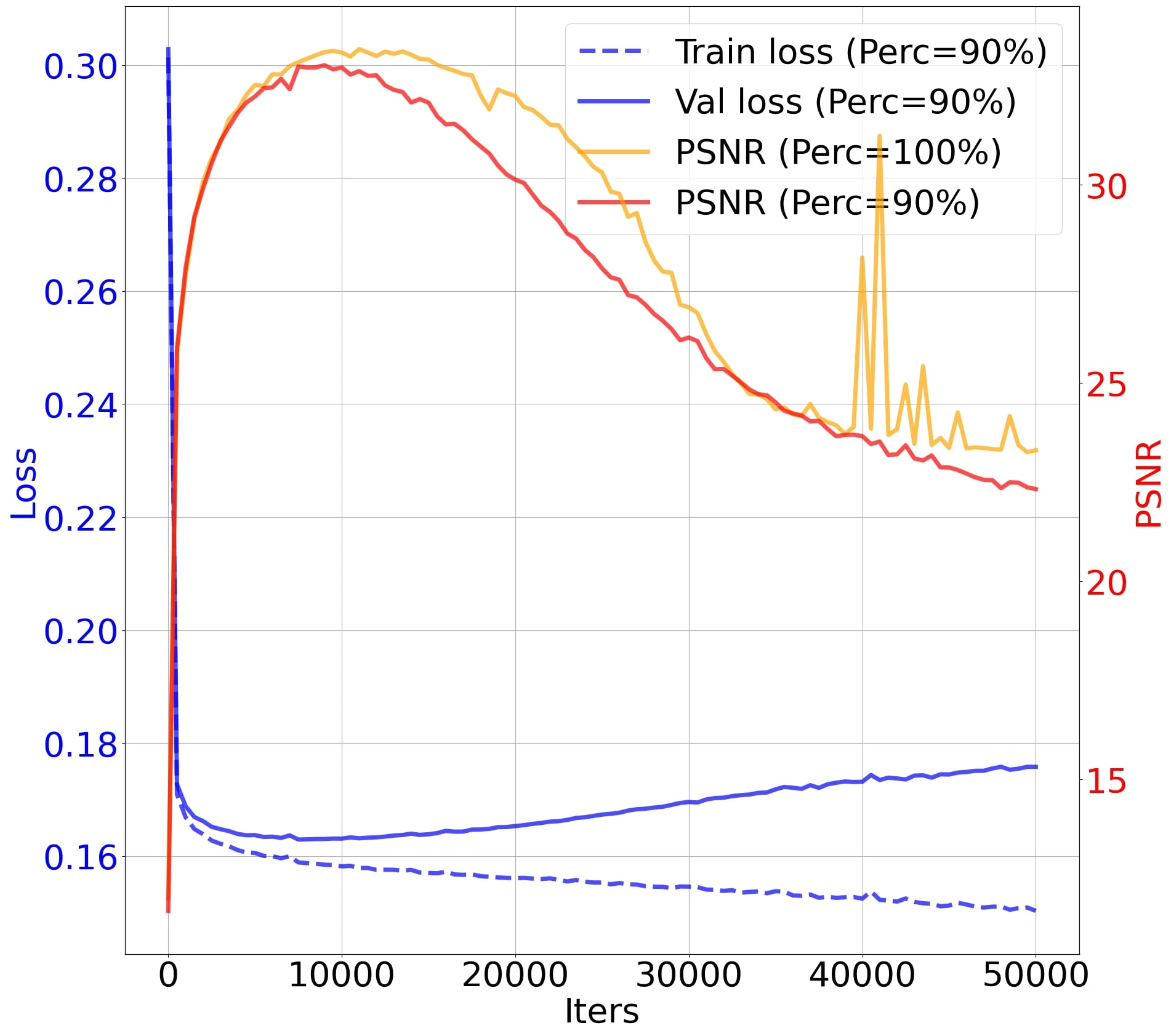
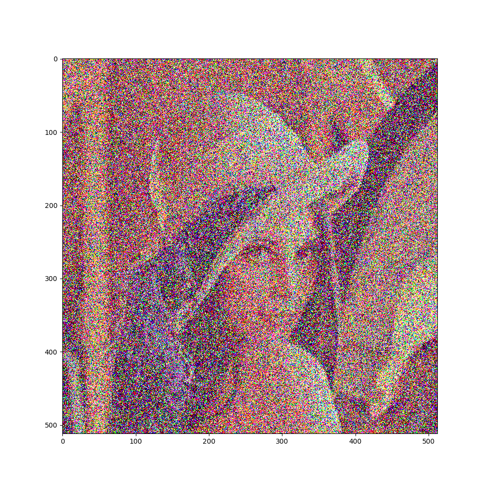
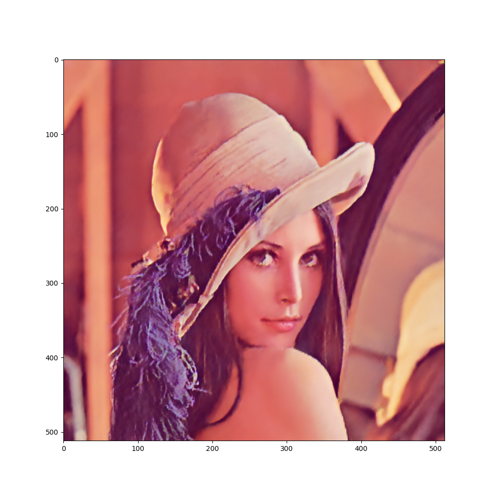
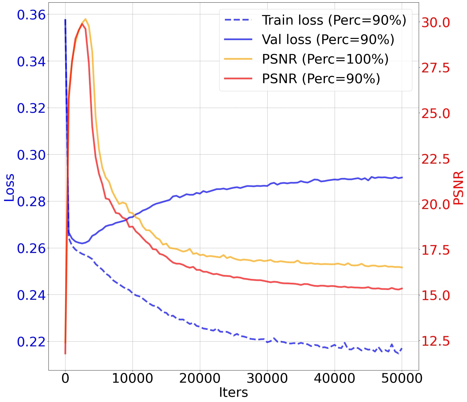
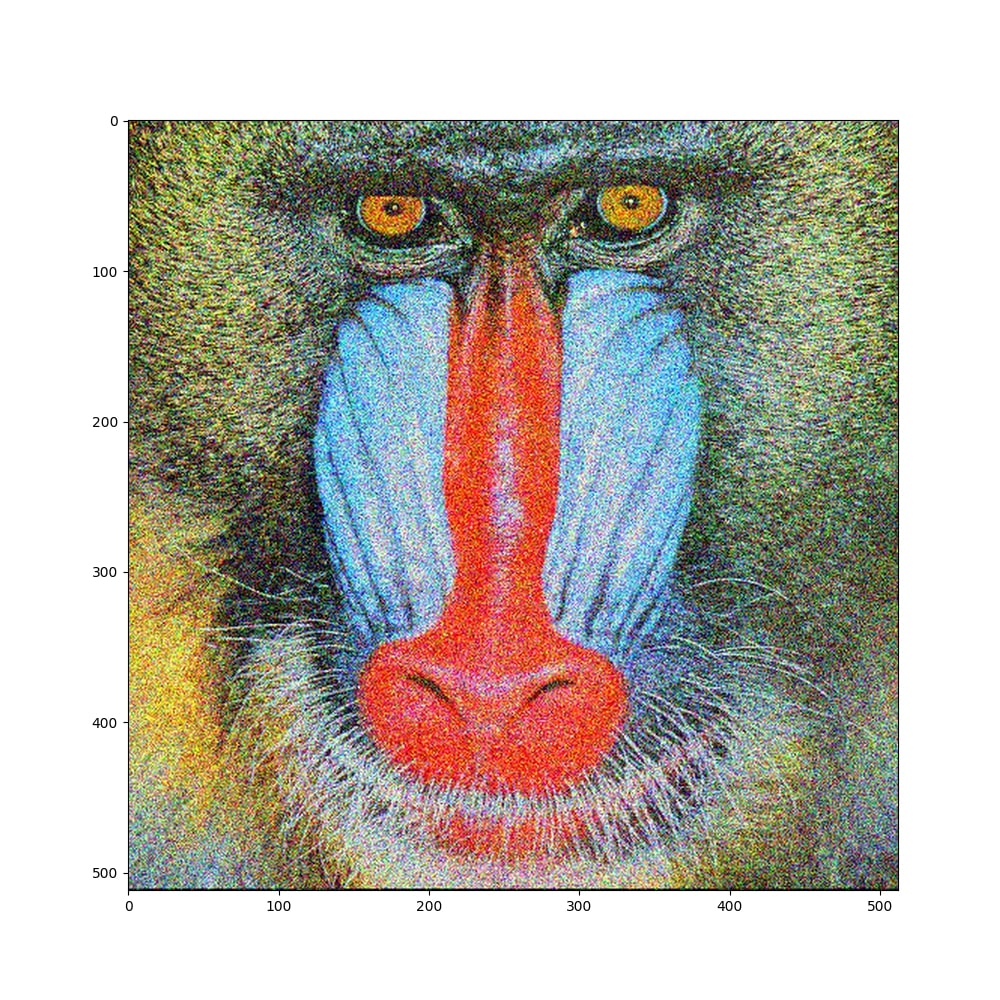
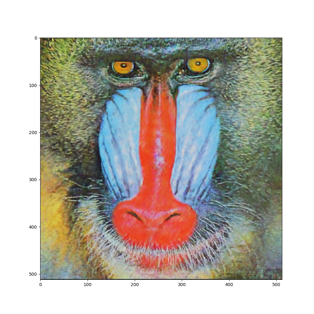
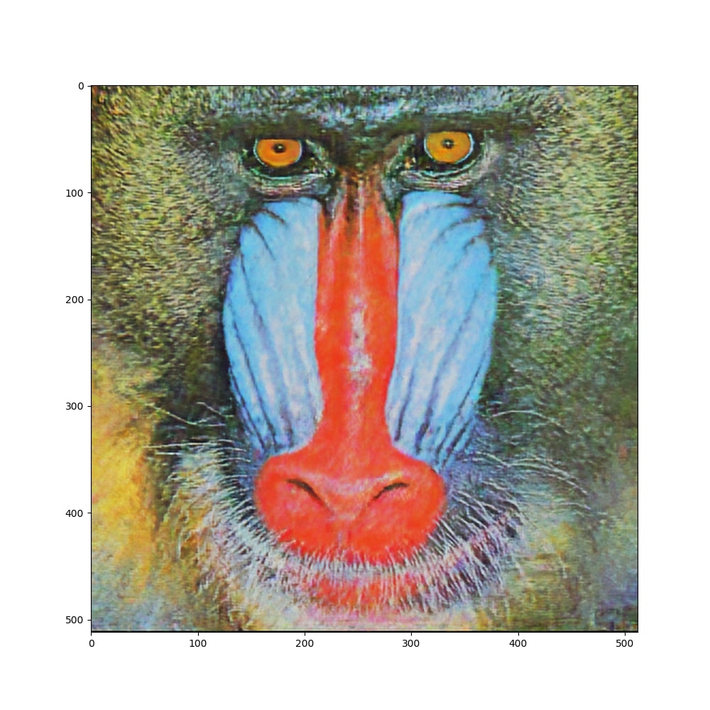
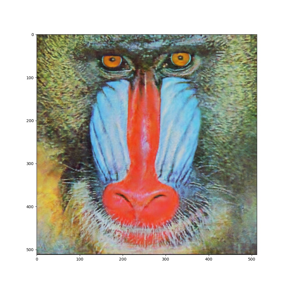
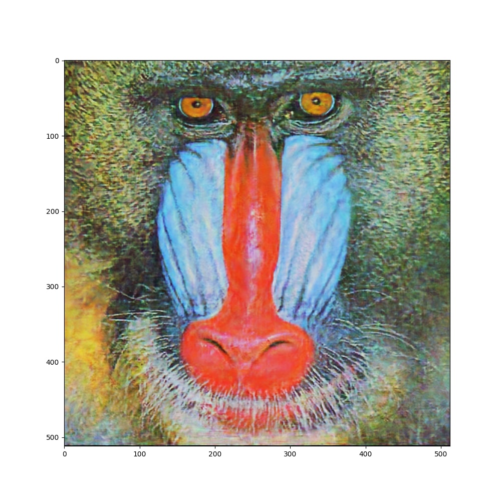
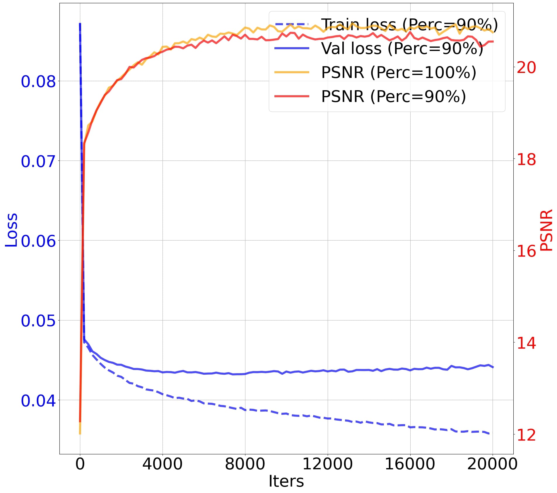
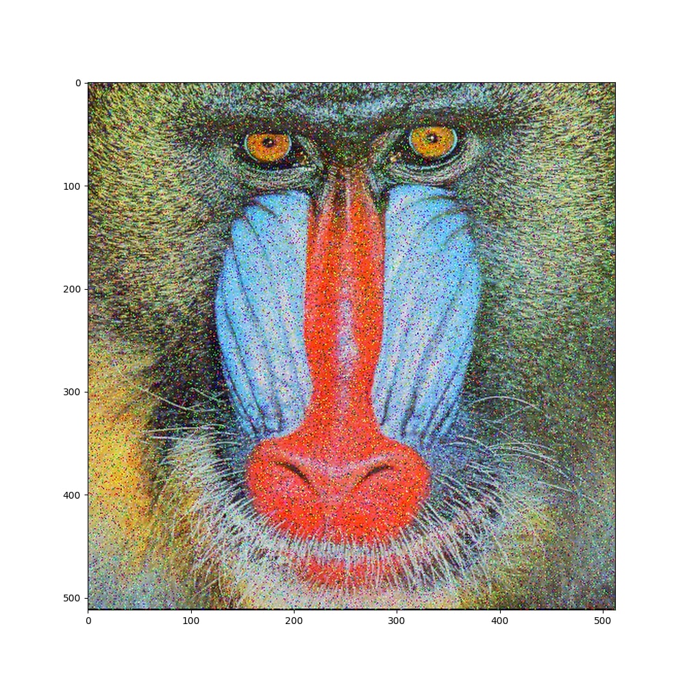
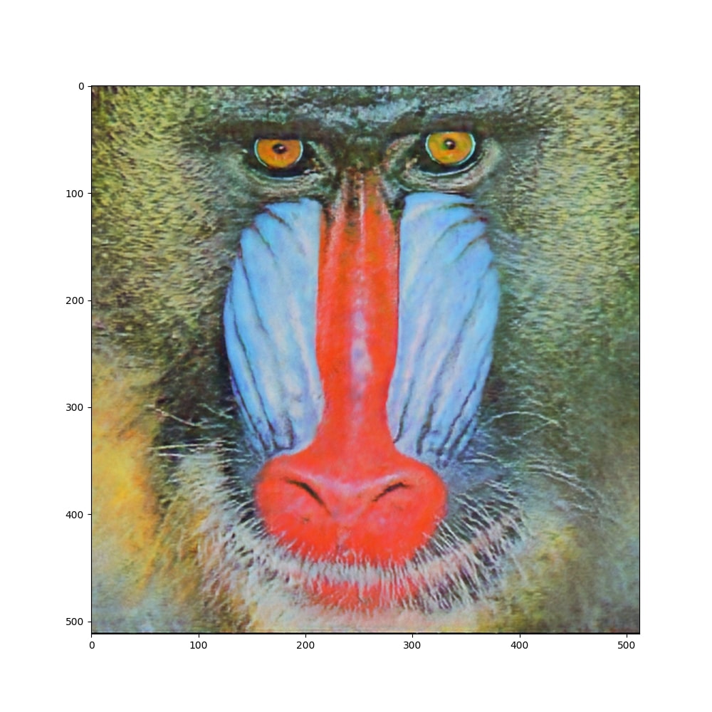
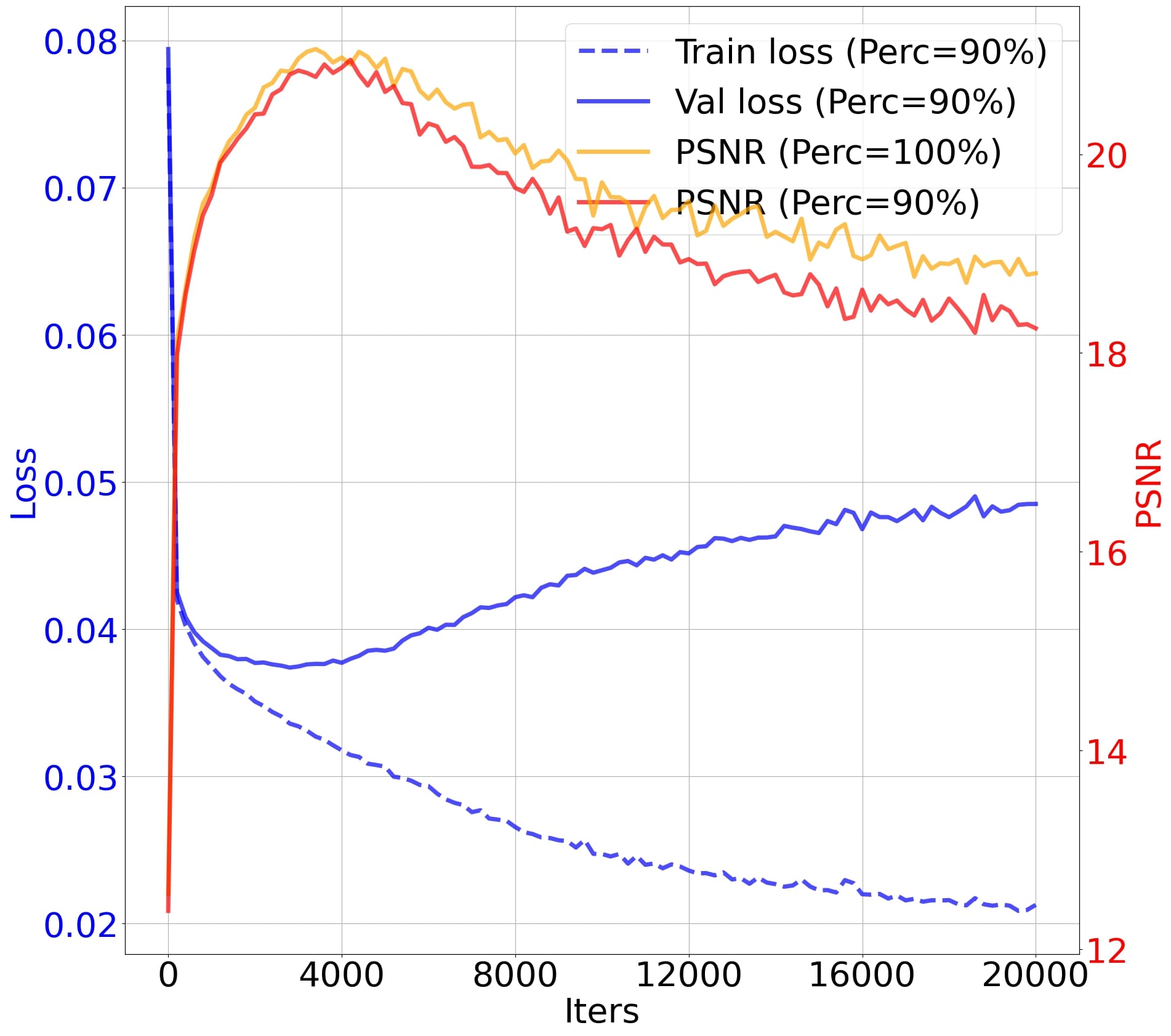
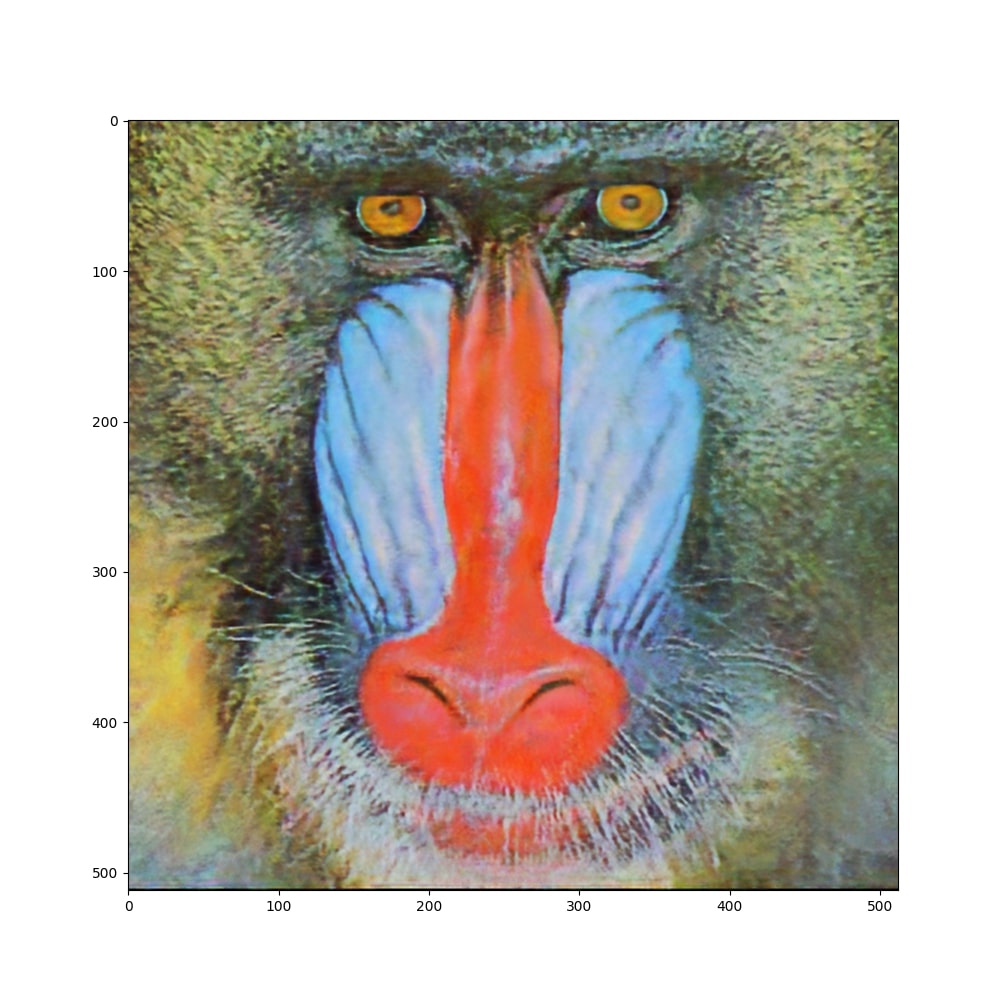
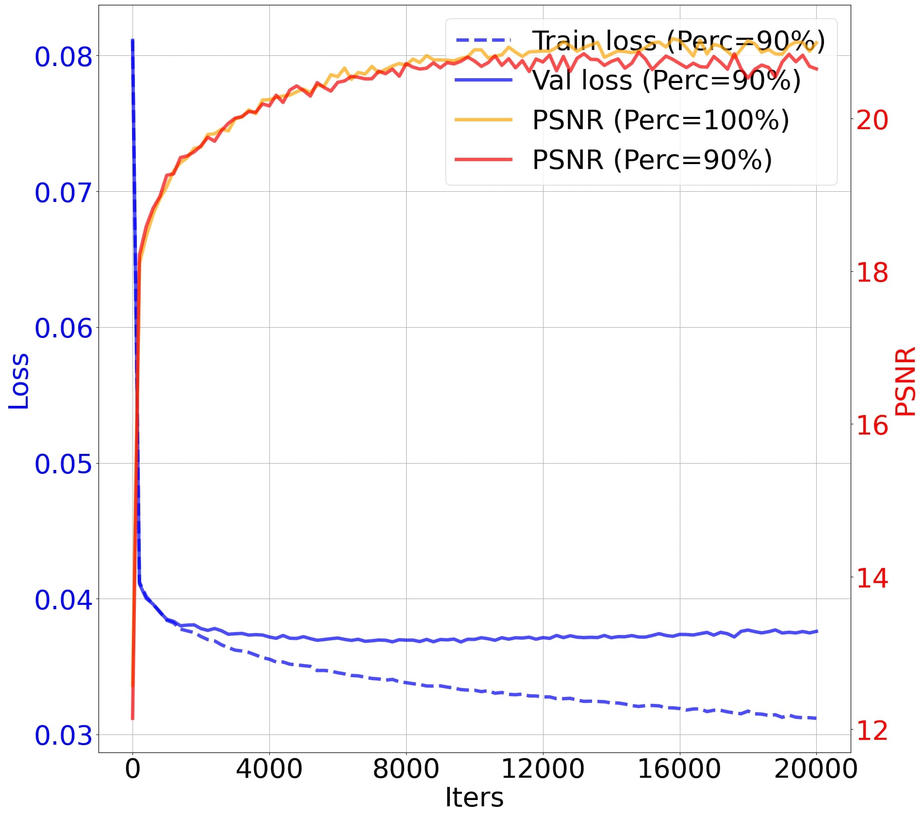
In the last set of experiments, we test the performance of the validation approach on image restoration with deep image prior. We follow the experiment setting as the work [25, 37] for denoising task, except that we randomly hold out 10 percent of pixels to decide the images with best performance during the training procedure. Concretely, we train the identical UNet network on the normalized standard dataset with different types of optimizer, noise and loss. In particular, the images are corrupted by two types of noises: $(i)$ Gaussian noise with mean 0 and standard deviation from $0.1$ to $0.3$, and $(ii)$ salt and papper noise where a certain ration (between $10\%$ to $50\%$) of randomly chosen pixels are replaced with either 1 or 0. We use SGD with learning rate $5$ and Adam with learning rate $0.05$. We evaluate the PSNR and val loss on the hold-out pixels across all experiment settings.

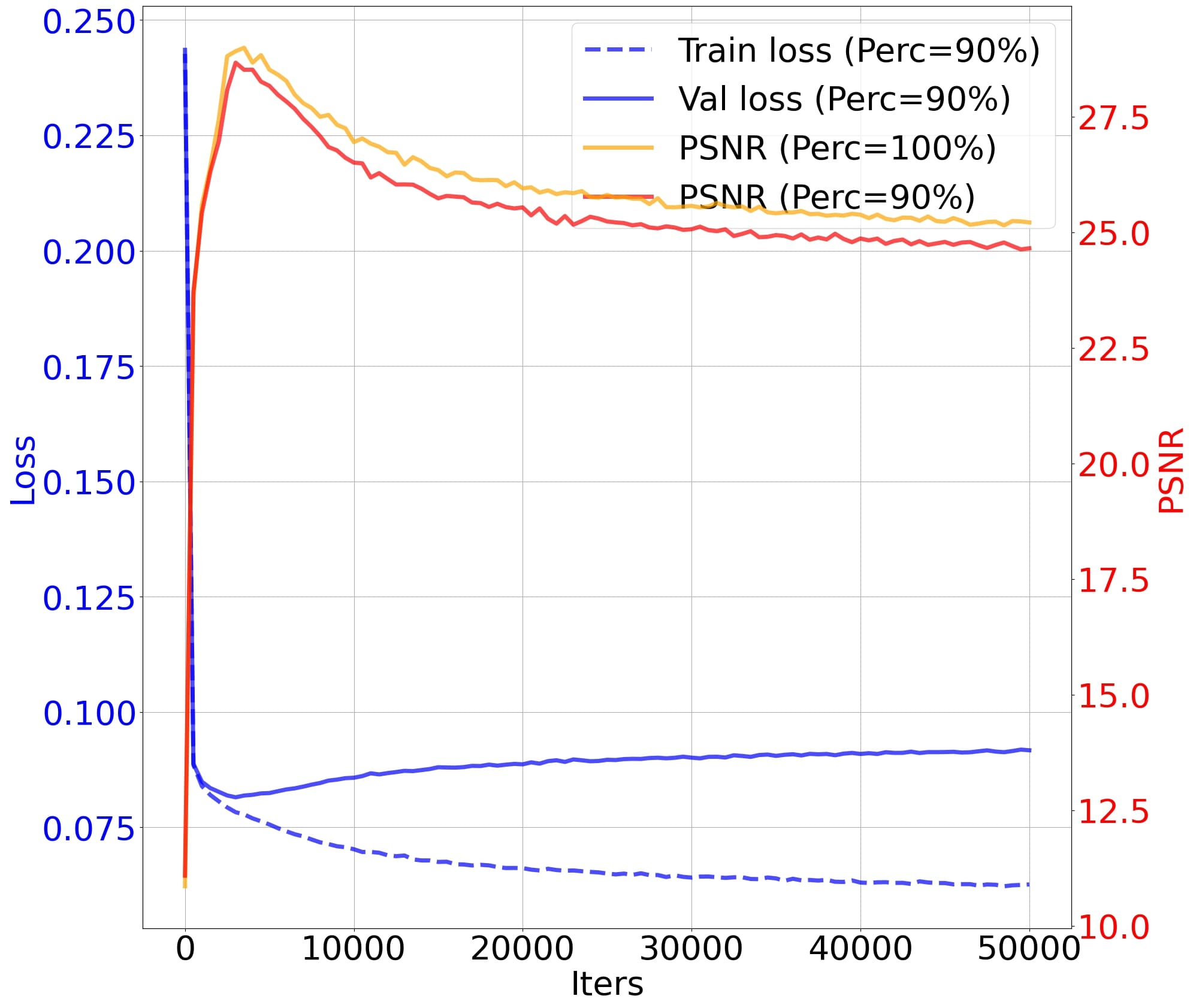
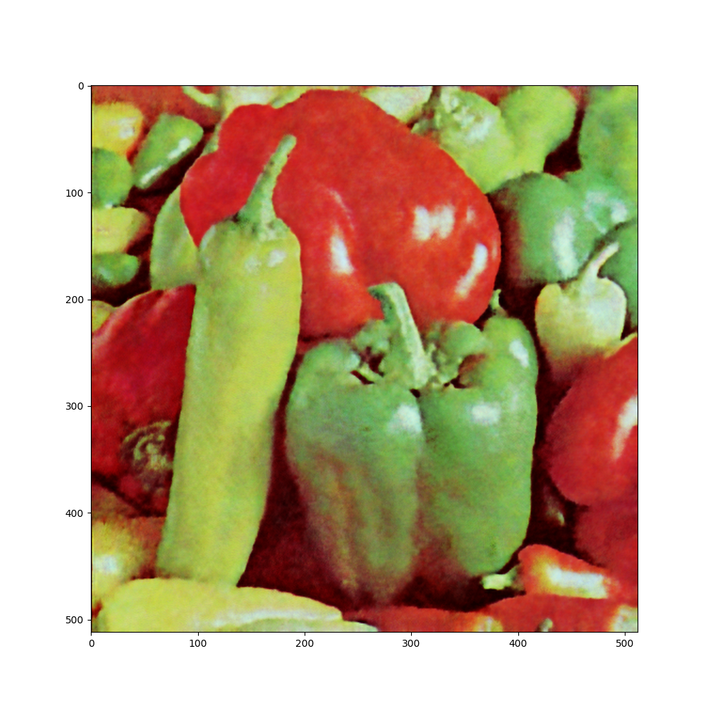
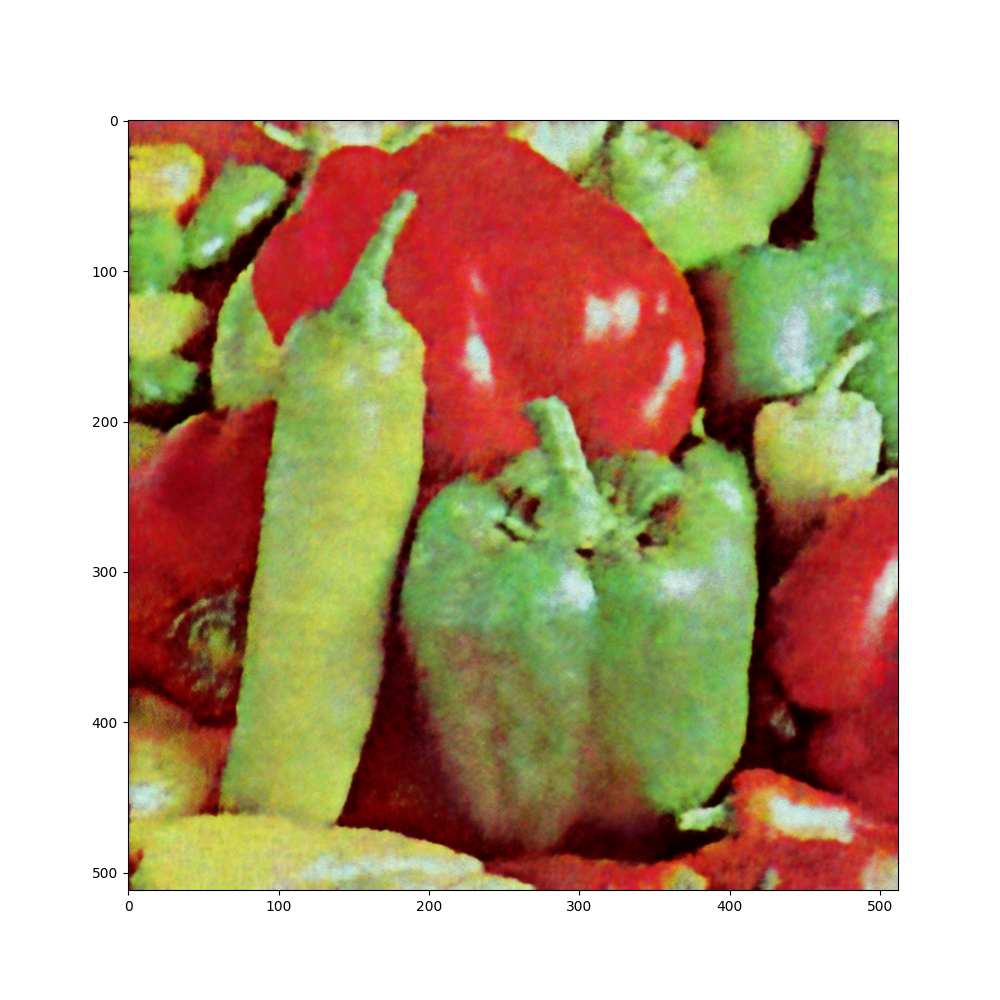
In Figure 3, we use Adam to train the network with L2 loss function for the Gaussian noise (at top row) and the salt and pepper noise (at bottom row) for 5000 iterations. From left to right, we plot the noisy image, the image with the smallest validation loss, the image with the best PSNR w.r.t. ground-truth image, and the learning curves, and the dynamic of training progress. We observe that for the case with Gaussian noise in the top row, our validation approach finds an image with PSNR $30.1544$, which is close to the best PSNR $30.2032$ through the entire training progress. Similar phenomenon also holds for salt and pepper noise, for which our validation approach finds an image with PSNR $25.7735$, which is close to the best PSNR $25.8994$. We note that finding the image with best PSNR is impractical without knowing the ground-truth image. On the other hand, as shown in the learning curves, the network overfitts the noise without early stopping. Finally, one may wonder without the holding out 10 percent of pixels will decreases the performance. To answer this question, we also plot the learning curves (orange lines) in Figure 3 (d) and (h) for training the UNet with entire pixels. We observe that the PSNR will only be improved very slightly by using the entire image, achieving PSNR $30.6762$ for Gaussian noise and PSNR $26.0728$ for salt-and-pepper noise. We observe similar results on different images, loss functions, and noise levels; see supplemental material for more results.

5 Conclusion

We analyzed gradient descent for the noisy over-parameterized matrix recovery problem where the rank is overspecified and the global solutions overfit the noise and do not correspond to the ground truth matrix. Under the restricted isometry property for the measurement operator, we showed that gradient descent with a validation approach achieves nearly information-theoretically optimal recovery.

An interesting question would be whether it is possible to extend our analysis to a non-symmetric matrix $X_{\natural}$, for which we need to optimize over two factors $U$ and $V$. In addition, it is of interest to extend our analysis for the matrix completion problem, as supported by the experiments in (4).

Appendix A Proof of Theorem 2.4

In this section, we prove our main result Theorem 2.4. We first present the proof strategy. Next, we provide detailed lemmas in characterizing the three phases described in the strategy. Theorem 2.4 then follows immediately from these lemmas.

For the ease of the presentation, in the following sections, we absorb the additional $\frac{1}{\sqrt{m}}$ factor into $\mathcal{A}$ and that the linear map $\mathcal{A}$ satisfies $(k,\delta)$-RIP means that

$$\frac{\left\|\mathcal{A}(X)\right\|_{2}^{2}}{\|X\|_{F}^{2}}\in[1-\delta,1+\delta],\quad\forall\,X~{}\text{ with}~{}\operatorname{rank}(X)\leq k.$$

We also decompose $X_{\natural}=U_{\natural}U_{\natural}^{\top}$. We write $\kappa_{f}=\frac{\sigma_{1}(U_{\natural})}{\sigma_{r_{\natural}}(U_{\natural})}$. Note that $\kappa_{f}^{2}=\kappa$. We define the noise matrix $E=\mathcal{A}^{*}(e)$.

A.1 Proof strategy

Our proof is largely based on [24], which deals with the case $E=0$, with a careful adjustment in handling the extra error caused by the noise matrix $E$. In this section, we outline the proof strategy and explain our contribution in dealing with the issues of the presence of noise. The main strategy is to show a signal term converges to $X_{\natural}$ up to some error while a certain error term stays small. To make the above precise, we present the following decomposition of $U_{t}$.

Decomposition of $U_{t}$

Consider the matrix $V_{X_{\natural}}^{\top}U_{t}\in\mathbb{R}^{r_{\natural}\times r}$ and its singular value decomposition $V_{X_{\natural}}^{\top}U_{t}=V_{t}\Sigma_{t}W_{t}^{\top}$ with $W_{t}\in\mathbb{R}^{r\times r_{\natural}}$. Also denote $W_{t,\perp}\in\mathbb{R}^{r\times(r-r_{\natural})}$ as a matrix with orthnormal columns and is orthogonal to $W_{t}$. Then we may decompose $U_{t}$ into “signal term” and “error term”:

$$U_{t}=\underbrace{U_{t}W_{t}W_{t}^{\top}}_{\text{signal term}}+\underbrace{U_{t}W_{t,\perp}W_{t,\perp}^{\top}}_{\text{error term}}.$$ (11)

The above decomposition is introduced in [24, Section 5.1] and may look technical at the first sight as it involves singular value decomposition. A perhaps more natural way of decomposing $U_{t}$ is to split it according to the column space of the ground truth $X_{\natural}$ as done in [19, 26]:

$$U_{t}=V_{X_{\natural}}V_{X_{\natural}}^{\top}U_{t}+V_{X_{\natural}^{\perp}}V_{X_{\natural}^{\perp}}^{\top}U_{t}.$$ (12)

However, as we observed from the experiments (not shown here), with the small random initialization, though the signal term $V_{X_{\natural}}^{\top}U_{t}$ does increase at a fast speed, the error term $V_{X_{\natural}^{\perp}}^{\top}U_{t}$ could also increase and does not stay very small. Thus, with $2r_{\natural}$-RIP only, the analysis becomes difficult as $V_{X_{\natural}^{\perp}}^{\top}U_{t}$ could be potentially high rank and large in nuclear norm.

Critical quantities for the analysis

What kind of quantities shall we look at to analyze the convergence of $U_{t}U_{t}^{\top}$ to $X_{\natural}$? The most natural one perhaps is the distance measured by the Frobenius norm:

$$\left\|U_{t}U_{t}^{\top}-X_{\natural}\right\|_{\tiny\text{F}}.$$ (13)

However, in the initial stage of the gradient descent dynamic with small random initialization (3), this quantity is actually almost stagnant. As in [24], we further consider the following three quantities to enhance the analysis:

$$\sigma_{r_{\natural}}(U_{t}W_{t}) \text{(maginitude of signal term)},$$ (14)

$$\|U_{t}W_{t,\perp}\| \text{(maginitude of error term)},$$

$$\|V_{X_{\natural}^{\perp}}^{\top}V_{U_{t}W_{t}}\| \text{(alignment of column space between signal to ground truth)}.$$

Here we assume $U_{t}W_{t}$ is full rank which can be ensured at initial random initialization and proved by induction for the remaining iterates.

Four phases of the gradient descent dynamic (3)

Here we described the four phases of the evolution of (3) and how the corresponding quantities change. The first three phases will be rigorously proved in the appendices.

1. The first phase is called the alignment phase. In this stage, there is an alignment between column spaces of the signal $U_{t}W_{t}$ and the ground truth $X_{\natural}$, i.e., the quantity $\|V_{X_{\natural}^{\perp}}^{\top}V_{U_{t}W_{t}}\|$ decreases and becomes small. Moreover, the signal $\sigma_{r_{\natural}}(U_{t}W_{t})$ is larger than the error $\|U_{t}W_{t,\perp}\|$ at the end of the phase though both term are still as small as initialization.

2. The second phase is the signal increasing stage. The signal term $U_{t}W_{t}$ matches the scaling of $(X_{\natural})^{\frac{1}{2}}$ (i.e., $\sigma_{r_{\natural}}(U_{t}W_{t})\geq\frac{\sqrt{\sigma_{r_{\natural}}(X_{\natural})}}{10}$) at a geometric speed, while the error term $\|U_{t}W_{t,\perp}\|$ is almost as small as initialization and the column spaces of the signal $U_{t}W_{t}$ and the ground truth $X_{\natural}$ still align with each other.

3. The third phase is the local convergence phase. In this phase, the distance $\|U_{t}U_{t}^{\top}-X_{\natural}\|_{F}$ starts geometrically decreasing up to the statistical error. This is the place where the analysis deviates from the one in [24] due to the presence of noise. In this stage, both $\|U_{t}W_{t,\perp}\|$ and $\|V^{\top}_{X_{\natural}^{\perp}}V_{U_{t}W_{t}}\|$ are of similar magnitude as before.

4. The last phase is the over-fitting phase. Due to the presence of noise, the gradient descent method will fit the noise, and thus $\|U_{t}U_{t}^{\top}-X_{\natural}\|_{F}$ will increase and $U_{t}$ approaches an optimal solution of (2) which results in over-fitting.

In short, we observe that the first two phases behave similarly as the noiseless case and thus we omit the proof since they can be proved with the same approach as in [24]. But the third phase requires additional efforts in dealing with the noise matrix $E$. Next, we describe the effect of small random initialization and why $2r_{\natural}$-RIP is sufficient.

Blessing and curse of small random initialization

As mentioned after Theorem 2.3, we require the initial size to be very small. Since the error term increases at a much lower speed compared with the signal term, small initialization ensures that $U_{t}W_{t}W_{t}^{\top}U_{t}$ gets closer to $X_{\natural}$ while the error $U_{t}W_{t,\perp}$ stays very small. The smallness of the error in the later stage of the algorithm is a blessing of small initialization. However, since $\alpha$ is very small and the direction $U$ is random, initially, the signal $U_{t}W_{t}$ is also very weak compared to the size of $X_{\natural}$. The initial weak signal is a curse of small random initialization.

Why is $2r_{\natural}$-RIP enough?

Since we are handling $n\times r$ matrices, it is puzzling why in the end we only need $2r_{\natural}$ RIP of the map $\mathcal{A}$. As it shall become clear in the proof, the need of RIP is mainly for bounding $\|(\mathcal{I}-\frac{\mathcal{A}^{*}\mathcal{A}}{m})(X_{\natural}-U_{t}U_{t})\|$. With the decomposition (11), we have

$$\|(\mathcal{I}-{\mathcal{A}^{*}\mathcal{A}}{})(X_{\natural}-U_{t}U_{t})\|\leq \|(\mathcal{I}-{\mathcal{A}^{*}\mathcal{A}})(X_{\natural}-U_{t}W_{t}^{\top}W_{t}U_{t})\|+\|(\mathcal{I}-{\mathcal{A}^{*}\mathcal{A}}{})(U_{t}W_{t,\perp}^{\top}W_{t,\perp}U_{t})\|$$

$$\overset{(a)}{\leq} \delta\|X_{\natural}-U_{t}W_{t}^{\top}W_{t}U_{t}\|+\delta\|U_{t}W_{t,\perp}^{\top}W_{t,\perp}U_{t}\|_{\ast}.$$

Here in the inequality $(a)$, we use the spectral-to-Frobenius bound (5) for the first term and the spectral-to-nuclear bound (6) for the second term. Recall that the error term $U_{t}W_{t,\perp}$ is very small due to the choice of $\alpha$ and $X_{\natural}-U_{t}W_{t}^{\top}W_{t}U_{t}$ is the quantity of interest. Thus bounding $\|(\mathcal{I}-{\mathcal{A}^{*}\mathcal{A}}{})(X_{\natural}-U_{t}U_{t}^{\top})\|$ becomes feasible.

A.2 Characterizing the three phases

Our first lemma rigorously prove the behavior of the three quantities $\sigma_{r_{\natural}}(U_{t}W_{t})$, $\|V_{X_{\natural}^{\perp}}^{\top}V_{U_{t}W_{t}}\|$, and $\|U_{t}W_{t,\perp}\|$ at the end of the first phase. The proof can be obtained from [24, Section 8] by changing the iterated matrix $M=\mathcal{A}^{*}\mathcal{A}(X_{\natural})$ to $M=\mathcal{A}^{*}\mathcal{A}(X_{\natural})+E$ and using the assumption that $\|E\|\leq c_{1}\kappa_{f}^{-2}\sigma_{r_{\natural}}(X_{\natural})$ for some small $c_{1}$. Hence, we omit the details.

Lemma A.1.

[24, Lemma 8.7] Let $U\in\mathbb{R}^{n\times r}$ be a random matrix with i.i.d. entries with distribution $\mathcal{N}\left(0,1/\sqrt{r}\right)$ and let $0<\varepsilon<1$. Assume the linear map $\mathcal{A}$ satisfies $(2r_{\natural},\delta)$ RIP with $\delta\leq\frac{c_{1}}{\kappa_{f}^{4}\sqrt{r_{\natural}}}$ and the bound $\|E\|\leq c_{1}\kappa_{f}^{-2}\sigma_{r_{\natural}}(X_{\natural})$. Let $U_{0}=\alpha U$, where

$$\alpha^{2}\lesssim\begin{cases}\frac{\sqrt{\min\left\{r;n\right\}}\|U_{\natural}\|^{2}}{\kappa_{f}n^{3/2}}\left(\frac{\kappa_{f}^{2}}{c_{2}}\sqrt{\frac{n}{\min\left\{r;n\right\}}}\right)^{-12\kappa_{f}^{2}}\quad&\text{if }r\geq 2r_{\natural}\\ \frac{\|U_{\natural}\|^{2}}{n^{3/2}\kappa_{f}}\left(\frac{2\kappa_{f}^{2}\sqrt{rn}}{c_{2}\varepsilon}\right)^{-12\kappa_{f}^{2}}\varepsilon\quad&\text{if }r<2r_{\natural}\end{cases}.$$ (15)

Assume that the step size satisfies $\mu\leq c_{2}\kappa_{f}^{-2}\|U_{\natural}\|^{2}$. Then with probability at least $1-p$, where

$$p=\begin{cases}O\left(\exp\left(-\tilde{c}r\right)\right)\quad&\text{if }r\geq 2r_{\natural}\\ \left(\tilde{C}\varepsilon\right)^{r-r_{\natural}+1}+\exp\left(-\tilde{c}r\right)\quad&\text{if }r<2r_{\natural}\end{cases}$$

the following statement holds. After

$${t_{\star}}\lesssim\begin{cases}\frac{1}{\mu\sigma_{r_{\natural}}\left(U_{\natural}\right)^{2}}\cdot\ln\left(2\kappa_{f}^{2}\sqrt{\frac{n}{\min\left\{r;n\right\}}}\right)\quad&\text{if }r\geq 2r_{\natural}\\ \frac{1}{\mu\sigma_{r_{\natural}}\left(U_{\natural}\right)^{2}}\cdot\ln\left(\frac{2\kappa_{f}^{2}\sqrt{rn}}{\varepsilon}\right)\quad&\text{if }r<2r_{\natural}\end{cases}$$

iterations it holds that

$$\|U_{t_{\star}}\| \leq 3\|U_{\natural}\|, \sigma_{\min}\left(U_{t_{\star}}W_{t_{\star}}\right) \geq\frac{\alpha\beta}{4},$$ (16)

$$\|U_{t_{\star}}W_{t_{\star},\perp}\| \leq\frac{\kappa_{f}^{-2}}{8}\alpha\beta, \|V_{X_{\natural}^{\perp}}^{T}V_{U_{t_{\star}}W_{t_{\star}}}\| \leq c\kappa_{f}^{-2},$$ (17)

where $\beta>0$ satisfies $\beta\lesssim\begin{cases}\frac{n\kappa_{f}^{4}}{c^{2}_{3}\left(\min\left\{r;n\right\}\right)}\quad&\text{if }r\geq 2r_{\natural}\\ \frac{n\kappa_{f}^{4}}{c^{2}_{3}\varepsilon}\quad&\text{if }r<2r_{\natural}\end{cases},\quad\text{and}\quad\beta\gtrsim\begin{cases}1\quad&\text{if }r\geq 2r_{\natural}\\ \frac{\varepsilon}{r}\quad&\text{if }r<2r_{\natural}\end{cases}.$ Here $c,c_{1},c_{2},c_{3},\tilde{C},\tilde{c}>0$ are absolute numerical constants.

The reason for the split of cases based on $2r_{\natural}$ is that this difference gives rise to the difference of the initial correlation between $U_{0}$ and the eigenspace of $M$ for the top $r_{\natural}$ eigenvalues.

The next lemma characterizes the behavior of the four quantities $\sigma_{r_{\natural}}(U_{t}W_{t})$, $\|V_{X_{\natural}^{\perp}}^{\top}V_{U_{t}W_{t}}\|$, $\|U_{t}W_{t,\perp}\|$, and $\|U_{t}U_{t}^{\top}-X_{\natural}\|_{F}$ in the end of the second phase. The proof can be adapted from [24, Section 9] by replacing $\mathcal{I}-\mathcal{A}^{*}\mathcal{A}(M_{\natural}-U_{t}U_{t}^{\top})$ by $\mathcal{I}-\mathcal{A}^{*}\mathcal{A}(M_{\natural}-U_{t}U_{t}^{\top})+E$ so we omit the details.

Lemma A.2.

[24, Proof of Theorem 9.6, Phase II] Instate the assumption in Theorem 2.4. Let $\gamma>0$ and choose the iteration count $t_{\star}$ such that $\sigma_{\min}\left(U_{t_{\star}}W_{t_{\star}}\right)\geq\gamma$. Furthermore, assume that the following conditions hold for some small but universal $c_{1},c_{2}>0$:

$$\|U_{t_{\star}}W_{t_{\star},\perp}\| \leq 2\gamma, \|U_{t_{\star}}\|\leq 3\|U_{\natural}\|,$$ (18)

$$\gamma \leq c_{1}\frac{\sigma_{\min}\left(U_{\natural}\right)}{\min\left\{r;n\right\}\kappa_{f}^{2}}, \|V_{X_{\natural}^{\perp}}^{T}V_{U_{t_{\star}}W_{t_{\star}}}\|\leq c_{2}\kappa_{f}^{-2}.{\tiny}$$ (19)

Set $t_{1}:=\min\Big{\{}t\geq t_{\star}:\sigma_{\min}\big{(}V_{X_{\natural}}^{T}U_{t}\big{)}\geq\frac{\sigma_{\min}\left(U_{\natural}\right)}{\sqrt{10}}\Big{\}}$. Such a finite $t_{1}$ always exists and satisfies $t_{1}-t_{\star}\leq\frac{16}{\mu\sigma_{\min}^{2}\left(U_{\natural}\right)}\ln\big{(}\sqrt{\frac{5}{2}}\frac{\sigma_{\min}\left(U_{\natural}\right)}{\gamma}\big{)}.$ Then the following inequalities hold for each $t\in[t_{\star},t_{1}]$:

$$\sigma_{\min}\left(V_{X_{\natural}}^{T}U_{t}\right) \geq\frac{1}{2}\left(1+\frac{1}{8}\mu\sigma_{\min}^{2}\left(U_{\natural}\right)\right)^{t-t_{\star}}\gamma,$$ (20)

$$\|U_{t}W_{t,\perp}\| \leq 2\left(1+80\mu c_{2}\sigma_{\min}^{2}\left(U_{\natural}\right)\right)^{t-t_{\star}}\gamma,$$ (21)

$$\|U_{t}\| \leq 3\|U_{\natural}\|,\quad\text{and}\quad\|V_{M_{\natural}^{\perp}}^{T}V_{U_{t}W_{t}}\|\leq c_{2}\kappa_{f}^{-2}.$$ (22)

Different from the noiseless case, the iterate $U_{t}$ can only get close to $U_{\natural}$ up to a certain noise level due to the presence of noise. The following lemma characterizing the quantity $\|U_{t}U_{t}^{\top}-X_{\natural}\|_{F}$ and is our main technical endeavor. The proof can be found in Section A.4.

Lemma A.3.

Instate the assumptions and notations in Lemma A.2. If $r>r_{\natural}$, then after

$$\hat{t}-t_{1}\lesssim\frac{1}{\mu\sigma_{\min}\left(U_{\natural}\right)^{2}}\ln\left(\max\left\{1;\frac{16\kappa_{f}}{\min\left\{r;n\right\}-r_{\natural}}\right\}\frac{\|U_{\natural}\|}{\gamma}\right)$$ (23)

iterations it holds that

$$\frac{\|U_{\hat{t}}U_{\hat{t}}^{T}-X_{\natural}\|_{\tiny\mathrm{F}}}{\|U_{\natural}\|^{2}}\lesssim\frac{\left(\min\left\{r;n\right\}-r_{\natural}\right)^{3/4}r_{\natural}^{1/2}}{\kappa_{f}^{3/16}}\cdot\frac{\gamma^{21/16}}{\|U_{\natural}\|^{21/16}}+r_{\natural}^{1/2}\kappa_{f}^{2}\frac{\|E\|}{\|U_{\natural}\|^{2}}.$$

If $r=r_{\natural}$, then for any $t\geq t_{1}$, we have

$$\|U_{\hat{t}}U_{\hat{t}}^{T}-X_{\natural}\|_{\tiny\mathrm{F}}\lesssim r_{\natural}^{1/2}\left(1-\frac{\mu}{400}\sigma_{\min}\left(X\right)^{2}\right)^{t-t_{1}}\|U_{\natural}\|^{2}+r_{\natural}^{1/2}\|E\|\kappa_{f}^{2}.$$

A.3 Proof of Theorem 2.4

Theorem 2.4 can be proved by applying Lemma A.1 and A.2 and A.3. More specifically, we set $\varepsilon=\frac{1}{n}$ in Lemma A.1 and $\gamma=\frac{\alpha\beta}{4}$ for Lemmas A.2 and A.3. A few more algebra manipulations yield $\frac{\|U_{\hat{t}}U_{\hat{t}}^{\top}-X_{\natural}\|_{\tiny\mathrm{F}}}{\|X_{\natural}\|}\lesssim\frac{\alpha}{\sqrt{\|X_{\natural}\|}}+\sqrt{r_{\natural}}\kappa\frac{\|E\|}{\|X_{\natural}\|}.$

A.4 Proof of Lemma A.3

We start with a lemma showing that $U_{t}U_{t}^{T}$ converges towards $X_{\natural}$ up to some statistical error when projected onto the column space of $X_{\natural}$. The proof of the lemma can be found in Section A.5. It is an analog of [24, Lemma 9.5] with a careful adjustment of the norms and the associated quantities. See Footnote 4 for a detailed explanation.

Lemma A.4.

Assume that $\|U_{t}\|\leq 3\|U_{\natural}\|$, $\|E\|\leq\|U_{\natural}\|^{2}$, and $\sigma_{\min}\left(U_{t}W_{t}\right)\geq\frac{1}{\sqrt{10}}\sigma_{\min}\left(U_{\natural}\right)$. Moreover, assume that $\mu\leq c\kappa_{f}^{-2}\|U_{\natural}\|^{-2}$, $\|V_{X_{\natural}^{\perp}}^{T}V_{U_{t}W_{t}}\|\leq c\kappa_{f}^{-2}$, and

$$\|\left(\mathcal{I}-\mathcal{A}^{*}\mathcal{A}\right)\left(X_{\natural}-U_{t}U_{t}^{T}\right)\|\leq c\kappa_{f}^{-2}\left(\|X_{\natural}-U_{t}W_{t}W_{t}^{\top}U_{t}^{T}\|+\|U_{t}W_{t,\perp}W_{t,\perp}^{\top}U_{t}\|_{\ast}\right)$$ (24)

where the constant $c>0$ is chosen small enough. Then it holds that

$$\|V_{X_{\natural}}^{T}\left(X_{\natural}-U_{t+1}U_{t+1}^{T}\right)\|$$

$$\leq \left(1-\frac{\mu}{200}\sigma_{\min}^{2}\left(U_{\natural}\right)\right)\|V_{X_{\natural}}^{T}\left(X_{\natural}-U_{t}U_{t}^{T}\right)\|+\mu\frac{\sigma_{\min}^{2}\left(U_{\natural}\right)}{100}\|U_{t}W_{t,\perp}W_{t,\perp}^{T}U_{t}^{T}\|_{\ast}+18\mu\|U_{\natural}\|^{2}\|E\|.$$

Let us now prove Lemma A.3.

Proof of Lemma A.3.

Case $r>r_{\natural}$: Set $\hat{t}:=t_{1}+\Big{\lceil}\frac{300}{\mu\sigma_{\min}\left(U_{\natural}\right)^{2}}\ln\left(16\kappa_{f}^{1/4}\frac{1}{\min\left\{r;n\right\}-r_{\natural}}\frac{\|U_{\natural}\|^{7/4}}{\gamma^{7/4}}\right)\Big{\rceil}.$ We first state our induction hypothesis for $t_{1}\leq t\leq\hat{t}$:

$$\sigma_{\min}\left(U_{t}W_{t}\right)\geq \sigma_{\min}\left(V_{X_{\natural}}^{T}U_{t}\right)\geq\frac{\sigma_{\min}\left(U_{\natural}\right)}{\sqrt{10}},$$ (25)

$$\|U_{t}W_{t,\perp}\|\leq \left(1+80\mu c_{2}\sigma_{\min}^{2}\left(U_{\natural}\right)\right)^{t-t_{1}}\|U_{t_{1}}W_{t_{1},\perp}\|,$$ (26)

$$\|U_{t}\|\leq 3\|U_{\natural}\|,$$ (27)

$$\|V_{X_{\natural}^{\perp}}^{T}V_{U_{t}W_{t}}\|\leq c_{2}\kappa_{f}^{-2},$$ (28)

$$\|V_{X_{\natural}}^{T}\left(X_{\natural}-U_{t}U_{t}^{T}\right)\|\leq 10\left(1-\frac{\mu}{400}\sigma_{\min}^{2}\left(U_{\natural}\right)\right)^{t-t_{1}}\|U_{\natural}\|^{2}$$ (29)

$$+18\mu\|U_{\natural}\|^{2}\|E\|\sum_{\tau=t_{1}+1}^{t}\left(1-\frac{\mu}{200}\sigma_{\min}^{2}\left(U_{\natural}\right)\right)^{\tau-t_{1}-1}.$$

For $t=t_{1}$ we note the inequalities (25), (27), and (28) follow from Lemma A.2. The inequality (26) trivially holds for $t=t_{1}$. For $t=t_{1}$, the inequality (29) holds due to the following derivation:

$$\|V_{X_{\natural}}^{T}\left(X_{\natural}-U_{t_{1}}U_{t_{1}}^{T}\right)\| =\|V_{X_{\natural}}^{T}\left(X_{\natural}-U_{t_{1}}W_{t_{1}}W_{t_{1}}^{T}U_{t_{1}}^{T}\right)\| \leq\|X_{\natural}\|+\|U_{t_{1}}W_{t_{1}}W_{t_{1}}^{T}U_{t_{1}}^{T}\| \leq 10\|U_{\natural}\|^{2}.$$

The last step is due to $\|U_{t_{1}}W_{t_{1}}\|\leq\|U_{t_{1}}\|\leq 3\|U_{\natural}\|$ by (27).

Using triangle inequality, the bound for $\left\|\left(\mathcal{A}^{*}\mathcal{A}-\mathcal{I}\right)\left(X_{\natural}-U_{t}U_{t}^{T}\right)\right\|_{\text{\tiny op}}$ in [24, pp. 33], and the assumption on $E$, we see that

$$\left\|\left(\mathcal{A}^{*}\mathcal{A}-\mathcal{I}\right)\left(X_{\natural}-U_{t}U_{t}^{T}\right)+E\right\|_{\text{\tiny op}}\leq 40c_{1}\kappa_{f}^{-2}\sigma_{r_{\natural}}\left(U_{\natural}\right)^{2}.$$

The above inequality allows us to use the argument in [24, Section 9, Proof of Theorem 9.6, Phase III] to prove (25), (27), (26), (28). We omit the details.

Next, the inequality (24) in Lemma A.4 is satisfied due to (A.1). Thus we have that

$$\|V_{X_{\natural}}^{T}\left(X_{\natural}-U_{t+1}U_{t+1}^{T}\right)\|$$

$$\leq \left(1-\frac{\mu}{200}\sigma_{\min}\left(U_{\natural}\right)^{2}\right)\|V_{X_{\natural}}^{T}\left(X_{\natural}-U_{t}U_{t}^{T}\right)\|+\mu\frac{\sigma_{\min}\left(U_{\natural}\right)^{2}}{100}\|U_{t}W_{t,\perp}W_{t,\perp}^{T}U_{t}^{T}\|_{\ast}+18\mu\|U_{\natural}\|^{2}\|E\|$$

$$\overset{(a)}{\leq} 10\left(1-\frac{\mu}{200}\sigma_{\min}\left(U_{\natural}\right)^{2}\right)\left(1-\frac{\mu}{400}\sigma_{\min}\left(U_{\natural}\right)^{2}\right)^{t-t_{1}}\|U_{\natural}\|^{2}+\mu\frac{\sigma_{\min}\left(U_{\natural}\right)^{2}}{100}\|U_{t}W_{t,\perp}W_{t,\perp}^{T}U_{t}^{T}\|_{\ast}$$

$$+18\mu\|U_{\natural}\|^{2}\|E\|\sum_{\tau=t_{1}+1}^{t+1}\left(1-\frac{\mu}{200}\sigma_{\min}\left(U_{\natural}\right)^{2}\right)^{\tau-t_{1}-1},$$

where in step (a), we use the induction hypothesis (29). Now (29) holds for $t+1$ if the following holds.

$$\|U_{t}W_{t,\perp}W_{t,\perp}^{T}U_{t}^{T}\|_{\ast}\leq\frac{1}{4}\left(1-\frac{\mu}{400}\sigma_{\min}\left(U_{\natural}\right)^{2}\right)^{t-t_{1}}\|U_{\natural}\|^{2}.$$ (30)

Using the relationship between operator norm and nuclear norm, we have

$$\|U_{t}W_{t,\perp}W_{t,\perp}^{T}U_{t}^{T}\|_{\ast} \leq(\min\left\{r;n\right\}-r_{\natural})\|U_{t}W_{t,\perp}\|^{2}$$

$$\overset{(a)}{\leq}4(\min\left\{r;n\right\}-r_{\natural})\left(1+80\mu c_{2}\sigma_{\min}\left(U_{\natural}\right)^{2}\right)^{2(t-t_{1})}\sigma_{\min}\left(U_{\natural}\right)^{1/4}\gamma^{7/4},$$

where in step $(a)$, we use (26) and the term $4\sigma_{\min}\left(U_{\natural}\right)^{1/4}\gamma^{7/4}$ is due to (21) and

$$t_{1}-t_{\star}\leq\frac{16}{\mu\sigma_{\min}^{2}\left(U_{\natural}\right)}\ln\left(\sqrt{\frac{5}{2}}\frac{\sigma_{\min}\left(U_{\natural}\right)}{\gamma}\right).$$

Hence, the inequality (30) holds if $c_{2}>0$ is small enough and

$$16(\min\left\{r;n\right\}-r_{\natural})\sigma_{\min}\left(U_{\natural}\right)^{1/4}\gamma^{7/4}\leq\left(1-\frac{\mu}{350}\sigma_{\min}\left(U_{\natural}\right)^{2}\right)^{t-t_{1}}\|U_{\natural}\|^{2}.$$

This is indeed true so long as $t\leq\hat{t}=t_{1}+\Big{\lceil}\frac{300}{\mu\sigma_{\min}\left(U_{\natural}\right)^{2}}\ln\left(16\kappa_{f}^{1/4}\frac{1}{\min\left\{r;n\right\}-r_{\natural}}\frac{\|U_{\natural}\|^{7/4}}{\gamma^{7/4}}\right)\Big{\rceil}$ by using the elementary inequality $\ln\left(1+x\right)\geq\frac{x}{1-x}$. This finishes the induction step for the case $r>r_{\natural}$.

Let us now verify the inequality for $\|U_{\hat{t}}U_{\hat{t}}^{T}-X_{\natural}\|_{\tiny\mathrm{F}}$ for $r>r_{\natural}$:

$$\|U_{\hat{t}}U_{\hat{t}}^{T}-X_{\natural}\|_{\tiny\mathrm{F}}\overset{(a)}{\leq} 4\|V_{X_{\natural}}^{T}\left(X_{\natural}-U_{\hat{t}}U_{\hat{t}}^{T}\right)\|_{\tiny\mathrm{F}}+\|U_{\hat{t}}W_{\hat{t},\perp}W_{\hat{t},\perp}^{T}U_{\hat{t}}^{T}\|_{\ast}$$ (31)

$$\overset{(b)}{\lesssim} r_{\natural}^{1/2}\left(1-\frac{\mu}{400}\sigma_{\min}\left(U_{\natural}\right)^{2}\right)^{\hat{t}-t_{1}}\|U_{\natural}\|^{2}$$

$$+r_{\natural}^{1/2}\mu\|U_{\natural}\|^{2}\|E\|\sum_{\tau=t_{1}+1}^{\hat{t}}\left(1-\frac{\mu}{200}\sigma_{\min}\left(U_{\natural}\right)^{2}\right)^{\tau-t_{1}-1}$$

$$\overset{(c)}{\lesssim} r_{\natural}^{1/2}\left(\kappa_{f}^{1/4}\frac{1}{\min\left\{r;n\right\}-r_{\natural}}\frac{\|U_{\natural}\|^{7/4}}{\gamma^{7/4}}\right)^{-3/4}\|U_{\natural}\|^{2}+r_{\natural}^{1/2}\|E\|\kappa_{f}^{2}$$

$$\lesssim \kappa_{f}^{-3/16}r_{\natural}^{1/2}\left(\min\left\{r;n\right\}-r_{\natural}\right)^{3/4}\gamma^{21/16}\|U_{\natural}\|^{11/16}+r_{\natural}^{1/2}\|E\|\kappa_{f}^{2},$$

where inequality $(a)$ follows from Lemma A.5. Inequality $(b)$ follows from (29) and (30). The step $(c)$ is due to the definition of $\hat{t}$.

Finally, we need to show (23). This follows simply from the definition of

$$\hat{t}=t_{1}+\Big{\lceil}\frac{300}{\mu\sigma_{\min}\left(U_{\natural}\right)^{2}}\ln\left(16\kappa_{f}^{1/4}\frac{1}{\min\left\{r;n\right\}-r_{\natural}}\frac{\|U_{\natural}\|^{7/4}}{\gamma^{7/4}}\right)\Big{\rceil}$$

and $t_{1}-t_{\star}\lesssim\frac{1}{\mu\sigma_{\min}^{2}\left(U_{\natural}\right)}\ln\left(\frac{\sigma_{\min}\left(U_{\natural}\right)}{\gamma}\right)$.

Case $r=r_{\natural}$: We note that for $t=t_{1}$, we have $U_{t}=U_{t}W_{t}W_{t}^{\top}$ and $W_{t,\perp}=0$ because $\sigma_{r_{\natural}}(U_{t}W_{t})>0$ and $W_{t}$ is of size $r_{\natural}\times r_{\natural}$. Following almost the same procedure as before, we can prove the induction hypothesis (25) to (29) for any $t\geq t_{1}$ again with (26) replaced by $\|U_{t}W_{t,\perp}\|=0$. Since we can ignore the term $U_{t}W_{t,\perp}$ in (30), we have (29) for all $t\geq t_{1}$. Finally, to bound $\|U_{t}U_{t}^{T}-X_{\natural}\|_{\tiny\mathrm{F}}$, we can replace $\hat{t}$ by $t$ in the inequality chain (31) and stop at step $(b)$ and bound $r_{\natural}^{1/2}\mu\|U_{\natural}\|^{2}\|E\|\sum_{\tau=t_{1}+1}^{\hat{t}}\left(1-\frac{\mu}{200}\sigma_{\min}\left(U_{\natural}\right)^{2}\right)^{\tau-t_{1}-1}$ by $r_{\natural}^{1/2}\|E\|\kappa_{f}^{2}$. ∎

A.5 Proof of Lemma A.4

We start with the following technical result.

Lemma A.5.

Under the assumptions of Lemma A.4 the following inequalities hold:

$$\|V_{X_{\natural}^{\perp}}^{T}U_{t}U_{t}^{T}\| \leq 3\|V_{X_{\natural}}^{T}\left(X_{\natural}-U_{t}U_{t}^{T}\right)\|+\|U_{t}W_{t,\perp}W_{t,\perp}^{T}U_{t}^{T}\|,$$ (32)

$$\|X_{\natural}-U_{t}U_{t}^{T}\| \leq 4\|V_{X_{\natural}}^{T}\left(X_{\natural}-U_{t}U_{t}^{T}\right)\|+\|U_{t}W_{t,\perp}W_{t,\perp}^{T}U_{t}^{T}\|,$$ (33)

$$\|X_{\natural}-U_{t}W_{t}W_{t}^{\top}U_{t}^{T}\| \leq 4\|V_{X_{\natural}}^{T}\left(X_{\natural}-U_{t}U_{t}^{T}\right)\|.$$ (34)

Proof.

The first two inequalities are proved in [24, Lemma B.4]. To prove the last inequality, we first decompose $X_{\natural}-U_{t}W_{t}W_{t}^{\top}U_{t}^{T}$ as

$$X_{\natural}-U_{t}W_{t}W_{t}^{\top}U_{t}^{T}=V_{X_{\natural}}V_{X_{\natural}}^{\top}(X_{\natural}-U_{t}W_{t}W_{t}^{\top}U_{t}^{T})+V_{X_{\natural}^{\perp}}V_{X_{\natural}^{\perp}}^{\top}(X_{\natural}-U_{t}W_{t}W_{t}^{\top}U_{t}^{T}).$$ (35)

For the first term, we have

$$V_{X_{\natural}}V_{X_{\natural}}^{\top}(X_{\natural}-U_{t}W_{t}W_{t}^{\top}U_{t}^{T}) =V_{X_{\natural}}V_{X_{\natural}}^{\top}XX^{\top}-V_{X_{\natural}}V_{X_{\natural}}^{\top}U_{t}W_{t}W_{t}^{\top}U_{t}^{T}$$ (36)

$$\overset{(a)}{=}V_{X_{\natural}}V_{X_{\natural}}^{\top}XX^{\top}-V_{X_{\natural}}V_{X_{\natural}}^{\top}U_{t}U_{t}^{T}.$$

Here the step $(a)$ is due to [24, Lemma 5.1]. Thus we have $\|V_{X_{\natural}}V_{X_{\natural}}^{\top}(X_{\natural}-U_{t}W_{t}W_{t}^{\top}U_{t}^{T})\|\leq\|V_{X_{\natural}}^{\top}XX^{\top}-V_{X_{\natural}}^{\top}U_{t}U_{t}^{T}\|$. Our task is then to bound the second term of (35):

$$\|V_{X_{\natural}^{\perp}}V_{X_{\natural}^{\perp}}^{\top}(X_{\natural}-U_{t}W_{t}W_{t}^{\top}U_{t}^{T})\|$$ (37)

$$\leq \|V_{X_{\natural}^{\perp}}V_{X_{\natural}^{\perp}}^{\top}(X_{\natural}-U_{t}W_{t}W_{t}^{\top}U_{t}^{T})V_{X_{\natural}}\|+\|V_{X_{\natural}^{\perp}}V_{X_{\natural}^{\perp}}^{\top}(X_{\natural}-U_{t}W_{t}W_{t}^{\top}U_{t}^{T})V_{X_{\natural}^{\perp}}V_{X_{\natural}^{\perp}}^{\top}\|$$

$$\overset{(a)}{\leq} \|(X_{\natural}-U_{t}U_{t}^{T})V_{X_{\natural}}\|+\|V_{X_{\natural}^{\perp}}U_{t}W_{t}W_{t}U_{t}^{T}V_{X_{\natural}^{\perp}}\|.$$

The step $(a)$ is due to [24, Lemma 5.1]. For the second term $\|V_{X_{\natural}^{\perp}}U_{t}W_{t}W_{t}U_{t}^{T}V_{X_{\natural}^{\perp}}\|$, we have the following estimate:

$$\|V_{X_{\natural}^{\perp}}^{T}U_{t}W_{t}W_{t}^{T}U_{t}^{T}V_{X_{\natural}^{\perp}}\|$$ (38)

$$= \|V_{X_{\natural}^{\perp}}^{T}V_{U_{t}W_{t}}V_{U_{t}W_{t}}^{T}U_{t}W_{t}W_{t}^{T}U_{t}^{T}V_{X_{\natural}^{\perp}}\|$$

$$= \|V_{X_{\natural}^{\perp}}^{T}V_{U_{t}W_{t}}\left(V_{X_{\natural}}^{T}V_{U_{t}W_{t}}\right)^{-1}V_{X_{\natural}}^{T}V_{U_{t}W_{t}}V_{U_{t}W_{t}}^{T}U_{t}W_{t}W_{t}^{T}U_{t}^{T}V_{X_{\natural}^{\perp}}\|$$

$$\leq \|V_{X_{\natural}^{\perp}}^{T}V_{U_{t}W_{t}}\|\|\left(V_{X_{\natural}}^{T}V_{U_{t}W_{t}}\right)^{-1}\|\|V_{X_{\natural}}^{T}V_{U_{t}W_{t}}V_{U_{t}W_{t}}^{T}U_{t}W_{t}W_{t}^{T}U_{t}^{T}V_{X_{\natural}^{\perp}}\|.$$

Using [24, Lemma 5.1] again, we know $V_{X_{\natural}}^{T}V_{U_{t}W_{t}}V_{U_{t}W_{t}}^{T}U_{t}W_{t}W_{t}^{T}U_{t}^{T}V_{X_{\natural}^{\perp}}=V_{X_{\natural}}^{T}U_{t}U_{t}^{T}V_{X_{\natural}^{\perp}}$ $=V_{X_{\natural}}^{T}\left(X_{\natural}-U_{t}U_{t}^{T}\right)V_{X_{\natural}^{\perp}}$. We also have $\frac{\|V_{X_{\natural}^{\perp}}^{T}V_{U_{t}W_{t}}\|}{\sigma_{\min}\left(V_{X_{\natural}}^{T}V_{U_{t}W_{t}}\right)}\leq 2$ due to $\|V_{X_{\natural}^{\perp}}^{\top}V_{U_{t}W_{t}}\|\leq c\kappa_{f}^{-2}$. This is true by noting that $V_{U_{t}W_{t}}=V_{X_{\natural}}V_{X_{\natural}}^{\top}V_{U_{t}W_{t}}+V_{X_{\natural}^{\perp}}V_{X_{\natural}^{\perp}}^{\top}V_{U_{t}W_{t}}$ and $\sigma_{r^{\star}}(V_{X_{\natural}}^{\top}V_{U_{t}W_{t}})=\sigma_{r^{\star}}(V_{X_{\natural}}V_{X_{\natural}}^{\top}V_{U_{t}W_{t}})\overset{(a)}{\geq}\sigma_{r^{\star}}(V_{U_{t}W_{t}})-\|V_{X_{\natural}^{\perp}}V_{X_{\natural}^{\perp}}^{\top}V_{U_{t}W_{t}}\|=1-\|V_{X_{\natural}^{\perp}}^{\top}V_{U_{t}W_{t}}\|$, where the step $(a)$ is due to Weyl’s inequality. Thus, the proof is completed by continuing the chain of inequality of (LABEL:eq:_intermediateLemma6.2):

$$\|V_{X_{\natural}^{\perp}}^{T}U_{t}W_{t}W_{t}^{T}U_{t}^{T}V_{X_{\natural}^{\perp}}\| \leq\frac{\|V_{X_{\natural}^{\perp}}^{T}V_{U_{t}W_{t}}\|}{\sigma_{\min}\left(V_{X_{\natural}}^{T}V_{U_{t}W_{t}}\right)}\|V_{X_{\natural}}^{T}\left(X_{\natural}-U_{t}U_{t}^{T}\right)V_{X_{\natural}^{\perp}}\|$$

$$\leq 2\|V_{X_{\natural}}^{T}\left(X_{\natural}-U_{t}U_{t}^{T}\right)\|.$$

∎

Let us now prove Lemma A.4.

Proof of Lemma A.4.

As in [24, Proof of Lemma 9.5], we can decompose $X_{\natural}-U_{t+1}U_{t+1}^{\top}$ into five terms by using the formula $U_{t+1}=U_{t}+\mu\left[\left(\mathcal{A}^{*}\mathcal{A}\right)\left(X_{\natural}-U_{t}U_{t}^{T}\right)+E\right]U_{t}$:

$$X_{\natural}-U_{t+1}U_{t+1}^{T}= \underset{{=(I)}}{\underbrace{\left(\mathcal{I}-\mu U_{t}U_{t}^{T}\right)\left(X_{\natural}-U_{t}U_{t}^{T}\right)\left(\mathcal{I}-\mu U_{t}U_{t}^{T}\right)}}$$

$$+\mu\underset{{=(II)}}{\underbrace{\left[\left(\mathcal{I}-\mathcal{A}^{*}\mathcal{A}\right)\left(X_{\natural}-U_{t}U_{t}\right)+E\right]U_{t}U_{t}^{T}}}$$

$$+\mu\underset{{=(III)}}{\underbrace{U_{t}U_{t}^{T}\left[\left(\mathcal{I}-\mathcal{A}^{*}\mathcal{A}\right)\left(X_{\natural}-U_{t}U_{t}^{T}\right)+E\right]}}-\mu^{2}\underset{{=(IV)}}{\underbrace{U_{t}U_{t}\left(X_{\natural}-U_{t}U_{t}^{T}\right)U_{t}U_{t}^{T}}}$$

$$-\mu^{2}\underset{{=(V)}}{\underbrace{\left[\left(\mathcal{A}^{*}\mathcal{A}\right)\left(X_{\natural}-U_{t}U_{t}^{T}\right)+E\right]U_{t}U_{t}^{T}\left[\left(\mathcal{A}^{*}\mathcal{A}\right)\left(X_{\natural}-U_{t}U_{t}^{T}\right)+E\right]}}.$$

Let us bound each term.

Bounding $(I)$: [24, Estimation of $(I)$ in the proof of Lemma 9.5] ensures that

$$\|V_{X_{\natural}}^{T}[\left(\mathcal{I}-\mathcal{A}^{*}\mathcal{A}\right)\left(X_{\natural}-UU_{t}^{T}\right)]U_{t}U_{t}^{T}\|\leq\frac{\sigma_{\min}^{2}\left(U_{\natural}\right)}{1000}\left(\|V_{X_{\natural}}^{T}\left(X_{\natural}-UU_{t}^{T}\right)\|+\|U_{t}W_{t,\perp}W_{t,\perp}^{T}U_{t}^{T}\|\right).$$

Bounding $(II)$: From triangle inequality and submultiplicity of $\|\cdot\|$, we have

$$\|V_{X_{\natural}}^{T}\left[\left(\mathcal{I}-\mathcal{A}^{*}\mathcal{A}\right)\left(X_{\natural}-U_{t}U_{t}^{T}\right)+E\right]U_{t}U_{t}^{T}\|$$

$$\leq \left(\|\left(\mathcal{I}-\mathcal{A}^{*}\mathcal{A}\right)\left(X_{\natural}-U_{t}U_{t}^{T}\right)\|+\|V^{\top}_{X}E\|\right)\|U_{t}\|^{2}$$

$$\overset{(a)}{\leq} 3^{2}\left(\|\left(\mathcal{I}-\mathcal{A}^{*}\mathcal{A}\right)\left(X_{\natural}-U_{t}U_{t}^{T}\right)\|+\|V^{\top}_{X}E\|\right)\|U_{\natural}\|^{2}$$

$$\overset{(b)}{\leq} 3^{3}c\sigma_{\min}^{2}\left(U_{\natural}\right)\left(\|X_{\natural}-U_{t}W_{t}W_{t}^{\top}U_{t}^{T}\|+\|U_{t}W_{t,\perp}W_{t,\perp}^{\top}U_{t}\|_{\ast}\right)+9\|V_{X_{\natural}}^{\top}E\|\|U_{\natural}\|^{2}$$

$$\overset{(c)}{\leq} 4\cdot 3^{3}c\sigma_{\min}^{2}\left(U_{\natural}\right)\left(\|V_{X_{\natural}}^{T}\left(X_{\natural}-U_{t}U_{t}^{T}\right)\|+\|U_{t}W_{t,\perp}W_{t,\perp}^{T}U_{t}\|_{\ast}\right)+3^{2}\|V_{X_{\natural}}^{\top}E\|\|U_{\natural}\|^{2}.$$

In the step $(a)$, we use the assumption $\|U\|\leq 3\|U_{\natural}\|$, and in the step $(b)$, we use assumption (24). In the step $(c)$, we use Lemma A.5. By taking a small constant $c>0$, we have

$$\|V_{X_{\natural}}^{T}\left[\left(\mathcal{I}-\mathcal{A}^{*}\mathcal{A}\right)\left(X_{\natural}-UU_{t}^{T}\right)\right]U_{t}U_{t}^{T}\|$$

$$\leq \frac{1}{1000}\sigma_{\min}^{2}\left(U_{\natural}\right)\left(\|V_{X_{\natural}}^{T}\left(X_{\natural}-UU_{t}^{T}\right)\|+\|U_{t}W_{t,\perp}W_{t,\perp}^{T}U_{t}^{T}\|_{\ast}\right)+3^{2}\|V_{X_{\natural}}^{\top}E\|\|U_{\natural}\|^{2}.$$

Bounding $(III)$: We derive the following inequality similarly as bounding $(II)$:

$$\|V_{X_{\natural}}^{T}U_{t}U_{t}^{T}\left[\left(\mathcal{I}-\mathcal{A}^{*}\mathcal{A}\right)\left(X_{\natural}-U_{t}U_{t}^{T}\right)+E\right]\|$$

$$\leq \frac{1}{1000}\sigma_{\min}^{2}\left(U_{\natural}\right)\left(\|V_{X_{\natural}}^{T}\left(X_{\natural}-UU_{t}^{T}\right)\|+\|U_{t}W_{t,\perp}W_{t,\perp}^{T}U_{t}^{T}\|_{\ast}\right)+3^{2}\|E\|\|U_{\natural}\|^{2}.$$

Estimation of $(IV)$: [24, Estimation of $(IV)$ in the proof of Lemma 9.5] ensures that

$$\mu^{2}\|V_{X_{\natural}}^{T}U_{t}U_{t}^{T}\left(X_{\natural}-U_{t}U_{t}^{T}\right)U_{t}U_{t}^{T}\|$$

$$\leq\frac{\mu}{200}\sigma_{\min}^{2}\left(X\right)\|V_{X_{\natural}}^{T}\left(X_{\natural}-U_{t}U_{t}^{T}\right)\|+\mu\frac{\sigma_{\min}^{2}\left(U_{\natural}\right)}{1000}\|U_{t}W_{t,\perp}W_{t,\perp}^{T}U_{t}^{T}\|.$$

Estimation of $(V)$: First, we have the following bound:

$$\|\left(\mathcal{A}^{*}\mathcal{A}\right)\left(X_{\natural}-U_{t}U_{t}^{T}\right)\| \leq\|X_{\natural}-U_{t}U_{t}^{T}\|+\|\left[\left(\mathcal{I}-\mathcal{A}^{*}\mathcal{A}\right)\left(X_{\natural}-U_{t}U_{t}^{T}\right)\right]\|$$

$$\overset{(a)}{\leq}2\left(\|X_{\natural}-U_{t}W_{t}W_{t}^{\top}U_{t}^{T}\|+\|U_{t}W_{t,\perp}W_{t,\perp}^{\top}U_{t}\|_{\ast}\right),$$

where in step $(a)$ we have used the assumption (24). Again using the assumption (24), we can show that

$$\|\left(\mathcal{A}^{*}\mathcal{A}\right)\left(X_{\natural}-U_{t}U_{t}^{T}\right)\| \leq 2\left(\|X_{\natural}-U_{t}W_{t}W_{t}^{\top}U_{t}^{T}\|+\|U_{t}W_{t,\perp}W_{t,\perp}^{\top}U_{t}\|_{\ast}\right)$$

$$\overset{(a)}{\leq}2\left(2\|U_{\natural}\|^{2}+\|U_{t}\|^{2}\right).$$

In the step $(a)$, we use the assumption $\|U_{t}W_{t,\perp}W_{t,\perp}^{\top}U_{t}\|_{\ast}\leq\|U_{\natural}\|^{2}$. Thus we can bound the term $(V)$ as follows:

$$\|V_{X_{\natural}}^{T}\left[\left(\mathcal{A}^{*}\mathcal{A}\right)\left(X_{\natural}-U_{t}U_{t}^{T}\right)+E\right]U_{t}U_{t}^{T}\left[\left(\mathcal{A}^{*}\mathcal{A}\right)\left(X_{\natural}-U_{t}U_{t}^{T}\right)+E\right]\|$$

$$\leq \left(\|\left[\left(\mathcal{A}^{*}\mathcal{A}\right)\left(X_{\natural}-U_{t}U_{t}^{T}\right)\right]\|+\|E\|\right)\|U_{t}\|^{2}\left(\|\left(\mathcal{A}^{*}\mathcal{A}\right)\left(X_{\natural}-U_{t}U_{t}^{T}\right)\|+\|E\|\right)$$

$$\overset{(a)}{\leq} 4\left(\|X_{\natural}-U_{t}W_{t}W_{t}^{\top}U_{t}^{T}\|+\|U_{t}W_{t,\perp}W_{t,\perp}^{\top}U_{t}\|_{\ast}+\|E\|\right)\|U_{t}\|^{2}\left(2\|U_{\natural}\|^{2}+\|U_{t}\|^{2}+\|E\|\right)$$

$$\overset{(b)}{\leq} 6^{4}\left(\|X_{\natural}-U_{t}W_{t}W_{t}^{\top}U_{t}^{T}\|+\|U_{t}W_{t,\perp}W_{t,\perp}^{\top}U_{t}\|_{\ast}+\|E\|\right)\|U_{\natural}\|^{4}$$

$$\overset{(c)}{\leq} 4\cdot 6^{4}\left(\|V_{X_{\natural}}^{T}\left(X_{\natural}-U_{t}U_{t}^{T}\right)\|+\|U_{t}W_{t,\perp}W_{t,\perp}^{T}U_{t}^{T}\|_{\ast}+\|E\|\right)\|U_{\natural}\|^{4},$$

where in the step $(a)$, we used the estimates from above. The step $(b)$ is due to the assumption $\|U_{t}\|\leq 3\|U_{\natural}\|$ and $\|E\|\leq\|U_{\natural}\|^{2}$. In the step $(c)$, we used Lemma A.5. Thus, we have

$$\mu^{2}\|V_{X_{\natural}}^{T}\left[\left(\mathcal{A}^{*}\mathcal{A}\right)\left(X_{\natural}-U_{t}U_{t}^{T}\right)+E\right]U_{t}U_{t}^{T}\left[\left(\mathcal{A}^{*}\mathcal{A}\right)\left(X_{\natural}-U_{t}U_{t}^{T}\right)+E\right]\|$$

$$\overset{(a)}{\leq} \frac{\mu}{1000}\sigma_{\min}^{2}\left(X\right)\|V_{X_{\natural}}^{T}\left(X_{\natural}-U_{t}U_{t}^{T}\right)\|+\frac{\mu}{400}\sigma_{\min}^{2}\left(X\right)\|U_{t}W_{t,\perp}W_{t,\perp}^{T}U_{t}^{T}\|_{\ast}+\frac{\mu}{400}\sigma_{\min}^{2}\left(X\right)\|E\|,$$

where the step $(a)$ is due to the assumption on the stepsize $\mu\leq c\kappa_{f}^{-2}\|U_{\natural}\|^{-2}$.

Our proof is finished by combining the above bounds on $(I)-(V)$. ∎

Appendix B Additional Experiments on DIP

In Section 4.3, we present the validity of our hold-out method for determining the denoised image through the training progress across different types of noise. In this section, we further conduct extensive experiments to investigate and verify the universal effectiveness. In Section B.1, we demonstrate that validity of our method is not limited on Adam by the experiments on SGD. In Section B.2, we demonstrate that validity of our method also holds for L1 loss function. In Section B.3, we demonstrate that validity of our method also exists across a wide range of noise degree for both gaussian noise and salt and pepper noise.

B.1 Validty across different optimizers

In this part, we verify the success of our method exists across different types of optimizers for dfferent noise. We use Adam with learning rate $0.05$ (at the top row) and SGD with learning rate $5$ (at the bottom row) to train the network for recovering the noise images under L2 loss for 20000 iterations, where we evaluate the validation loss between generated images and corrupted images , and the PSNR between generated image and clean images every 200 iterations. In Figure 4, we show that both Adam and SGD work for Gaussian noise, where we use the Gaussian noise with mean 0 and variance 0.2. At the top row, we plot the results of recovering images optimized by Adam. The PSNR of chosen recovered image according to the validation loss is $20.7518$ at the second column, which is comparable to the Best PSNR $20.8550$ through the training progress at the third column. The best PSNR of full noisy image is $21.0714$ through the training progress at the last column. At the bottom row, we show the results of SGD, The PSNR of decided image according to the validation loss is $20.6964$ at the second column, which is comparable to the Best PSNR $20.7551$ through the training progress at the third column. The best PSNR of full noisy image is $20.9449$ through the training progress at the last column. In Figure 5, we show that both Adam and SGD works for salt and pepper noise, where $10\%$ percent of pixels are randomly corrupted. At the top row, we plot the results of recovering images optimized by Adam. The PSNR of chosen recovered image according to the validation loss is $20.8008$ at the second column, which is comparable to the Best PSNR $20.9488$ through the training progress at the third column. The best PSNR of full noisy image is $21.0576$ through the training progress at the last column. At the bottom row, we show the results of SGD, The PSNR of decided image according to the validation loss is $20.7496$ at the second column, which is comparable to the Best PSNR $20.8691$ through the training progress at the third column. The best PSNR of full noisy image is $21.0461$ through the training progress at the last column. Comparing these results, the SGD optimization algorithm usually takes more iterations to recovery the noisy images corrupted by either Gaussian noise and salt and pepper noise, therefore we will use Adam in the following parts.

(a)

(b)

(c)

(d)

(e)

(f)

(g)

(h)

Figure 4: Results across different optimizer for guassian noise. The top row plots the results for Adam, and the bottom row plots the results for SGD.

(a)

(b)

(c)

(d)

(e)

(f)

(g)

(h)

Figure 5: Results across different optimizer for salt and pepper noise. The top row plots the results for Adam, and the bottom row plots the results for SGD.

B.2 Validty across loss functions

(a)

(b)

(c)

(d)

(e)

(f)

(g)

(h)

Figure 6: Results across different losses for guassian noise. The top row plots the results for L1 loss, and the bottom row plots the results for L2 loss.

(a)

(b)

(c)

(d)

(e)

(f)

(g)

(h)

Figure 7: Results across different losses for salt and pepper noise. The top row plots the results for L1 loss, and the bottom row plots the results for L2 loss.

In this part, we verify the success of our method exists across different types of loss functions for different noise. We use Adam with learning rate $0.05$ to train the network for recovering the noise images under either L1 loss (at the top row) or L2 loss (at the bottom row) for 50000 iterations, where we evaluate the validation loss between generated images and corrupted images, and the PSNR between generated image and clean images every 500 iterations. In Figure 6, we show that both L1 loss and L2 loss works for Gaussian noise, where we use the Gaussian noise with mean 0 and variance 0.2. At the top row, we plot the results of recovering images under L1 loss. The PSNR of chosen recovered image according to the validation loss is $27.5232$ at the second column, which is comparable to the Best PSNR $27.5233$ through the training progress at the third column. The best PSNR of full noisy image is $28.1647$ through the training progress at the last column. At the bottom row, we show the results under L2 loss, The PSNR of decided image according to the validation loss is $27.7941$ at the second column, which is comparable to the Best PSNR $27.9268$ through the training progress at the third column. The best PSNR of full noisy image is $27.9370$ through the training progress at the last column. In Figure 7, we show that both L1 loss and L2 loss works for salt and pepper noise, where $30\%$ percent of pixels are randomly corrupted. At the top row, we plot the results of recovering images optimized by Adam. The PSNR of chosen recovered image according to the validation loss is $35.2155$ at the second column, which is comparable to the Best PSNR $35.2266$ through the training progress at the third column. The best PSNR of full noisy image is $35.9319$ through the training progress at the last column. At the bottom row, we show the results of SGD, The PSNR of decided image according to the validation loss is $21.8679$ at the second column, which is comparable to the Best PSNR $21.8679$ through the training progress at the third column. The best PSNR of full noisy image is $22.1088$ through the training progress at the last column. Comparing these results, the L1 loss usually performs comparably as L2 loss to recovery the noisy images corrupted by either Gaussian noise, and L1 loss converges faster and produces cleaner recovered image than L2 loss for salt and pepper noise, therefore, we will use L1 loss in the following parts.

B.3 Validty across noise degree

In this part, we verify the success of our method exists across different noise degrees for different noise. We use Adam with learning rate $0.05$ to train the network for recovering the noise images under L1 loss for 50000 iterations, where we evaluate the validation loss between generated images and corrupted images, and the PSNR between generated image and clean images every 500 iterations. In Figure 8, we show that our methods works for different noise degree of Gaussian noise, where we use the Gaussian noise with mean 0. At the top row, we plot the results of recovering images under 0.1 variance of gaussian noise. The PSNR of chosen recovered image according to the validation loss is $28.6694$ at the second column, which is comparable to the Best PSNR $28.6694$ through the training progress at the third column. The best PSNR of full noisy image is $28.9929$ through the training progress at the last column. At the middel row, we plot the results of recovering images under 0.2 variance of gaussian noise. The PSNR of chosen recovered image according to the validation loss is $25.6036$ at the second column, which is comparable to the Best PSNR $25.6839$ through the training progress at the third column. The best PSNR of full noisy image is $25.8879$ through the training progress at the last column. At the bottom row, we show the results under under 0.3 variance of gaussian noise, The PSNR of decided image according to the validation loss is $27.7784$ at the second column, which is identical to the Best PSNR $23.7784$ through the training progress at the third column. The best PSNR of full noisy image is $23.9001$ through the training progress at the last column. In Figure 9, we show that our methods works for different noise degree of salt and pepper noise. At the top row, we plot the results of recovering images with 10 percent of pixels randomly corrupted by salt and pepper noise. The PSNR of chosen recovered image according to the validation loss is $35.3710$ at the second column, which is comparable to the Best PSNR $35.5430$ through the training progress at the third column. The best PSNR of full noisy image is $35.9778$ through the training progress at the last column. At the middel row, we plot the results of recovering images under 30 percent of pixels randomly corrupted by salt and pepper noise. The PSNR of chosen recovered image according to the validation loss is $32.9904$ at the second column, which is comparable to the Best PSNR $33.0188$ through the training progress at the third column. The best PSNR of full noisy image is $33.4267$ through the training progress at the last column. At the bottom row, we show the results under 50 percent of pixels randomly corrupted by salt and pepper noise The PSNR of decided image according to the validation loss is $29.8836$ at the second column, which is identical to the Best PSNR $29.8836$ through the training progress at the third column. The best PSNR of full noisy image is $20.1512$ through the training progress at the last column. Comparing both the results of gaussian noise and salt and pepper noise, we can draw three conclusion. First, the PSNR of recovered image drops with the noise degree increases. Second, The peak of PSNR occurs earlier with the noise degree increases. Last, the neighbor near the peak of PSNR becomes shaper with the noise degree increases.

(a)

(b)

(c)

(d)

(e)

(f)

(g)

(h)

(i)

(j)

(k)

(l)

Figure 8: Results across noise degree for gaussian noise. The top row plots the results for gaussian noise with mean 0 and variance 0.1, the middle row plots the results for gaussian noise with mean 0 and variance 0.2, and the bottom row plots the result for gaussian noise with mean 0 and variance 0.3.

(a)

(b)

(c)

(d)

(e)

(f)

(g)

(h)

(i)

(j)

(k)

(l)

Figure 9: Results across noise degree for salt and pepper noise. The top row plots the results for 10 percent of corrupted pixels, the middle row plots the results for 30 percent of corrupted pixels, and the bottom row plots the result for 50 percent of corrupted pixels.

References

• [1] Benjamin Recht, Maryam Fazel, and Pablo A Parrilo. Guaranteed minimum-rank solutions of linear matrix equations via nuclear norm minimization. SIAM review, 52(3):471–501, 2010.
• [2] E. J. Cand$\grave{\rm e}$s and Y. Plan. Tight oracle inequalities for low-rank matrix recovery from a minimal number of noisy random measurements. IEEE Trans. Inf. Theory, 57(4):2342–2359, Apr. 2011.
• [3] Yi-Kai Liu. Universal low-rank matrix recovery from pauli measurements. Advances in Neural Information Processing Systems, 24, 2011.
• [4] Steven T Flammia, David Gross, Yi-Kai Liu, and Jens Eisert. Quantum tomography via compressed sensing: error bounds, sample complexity and efficient estimators. New Journal of Physics, 14(9):095022, 2012.
• [5] Yuejie Chi, Yue M Lu, and Yuxin Chen. Nonconvex optimization meets low-rank matrix factorization: An overview. IEEE Transactions on Signal Processing, 67(20):5239–5269, 2019.
• [6] Prateek Jain, Praneeth Netrapalli, and Sujay Sanghavi. Low-rank matrix completion using alternating minimization. In Proceedings of the forty-fifth annual ACM symposium on Theory of computing, pages 665–674, 2013.
• [7] Ruoyu Sun and Zhi-Quan Luo. Guaranteed matrix completion via nonconvex factorization. In Foundations of Computer Science (FOCS), 2015 IEEE 56th Annual Symposium on, pages 270–289. IEEE, 2015.
• [8] Yudong Chen and Martin J Wainwright. Fast low-rank estimation by projected gradient descent: General statistical and algorithmic guarantees. arXiv preprint arXiv:1509.03025, 2015.
• [9] Srinadh Bhojanapalli, Behnam Neyshabur, and Nathan Srebro. Global optimality of local search for low rank matrix recovery. In Proceedings of the 30th International Conference on Neural Information Processing Systems, pages 3880–3888, 2016.
• [10] Stephen Tu, Ross Boczar, Max Simchowitz, Mahdi Soltanolkotabi, and Ben Recht. Low-rank solutions of linear matrix equations via procrustes flow. In International Conference on Machine Learning, pages 964–973. PMLR, 2016.
• [11] Rong Ge, Jason D Lee, and Tengyu Ma. Matrix completion has no spurious local minimum. arXiv preprint arXiv:1605.07272, 2016.
• [12] Rong Ge, Chi Jin, and Yi Zheng. No spurious local minima in nonconvex low rank problems: A unified geometric analysis. In International Conference on Machine Learning, pages 1233–1242. PMLR, 2017.
• [13] Zhihui Zhu, Qiuwei Li, Gongguo Tang, and Michael B Wakin. Global optimality in low-rank matrix optimization. IEEE Transactions on Signal Processing, 66(13):3614–3628, 2018.
• [14] Qiuwei Li, Zhihui Zhu, and Gongguo Tang. The non-convex geometry of low-rank matrix optimization. Information and Inference: A Journal of the IMA, 8(1):51–96, 2019.
• [15] Vasileios Charisopoulos, Yudong Chen, Damek Davis, Mateo Díaz, Lijun Ding, and Dmitriy Drusvyatskiy. Low-rank matrix recovery with composite optimization: good conditioning and rapid convergence. Foundations of Computational Mathematics, 21(6):1505–1593, 2021.
• [16] Haixiang Zhang, Yingjie Bi, and Javad Lavaei. General low-rank matrix optimization: Geometric analysis and sharper bounds. Advances in Neural Information Processing Systems, 34, 2021.
• [17] Samuel Burer and Renato DC Monteiro. A nonlinear programming algorithm for solving semidefinite programs via low-rank factorization. Mathematical Programming, 95(2):329–357, 2003.
• [18] Samuel Burer and Renato DC Monteiro. Local minima and convergence in low-rank semidefinite programming. Mathematical Programming, 103(3):427–444, 2005.
• [19] Jiacheng Zhuo, Jeongyeol Kwon, Nhat Ho, and Constantine Caramanis. On the computational and statistical complexity of over-parameterized matrix sensing. arXiv preprint arXiv:2102.02756, 2021.
• [20] Jialun Zhang, Salar Fattahi, and Richard Zhang. Preconditioned gradient descent for over-parameterized nonconvex matrix factorization. Advances in Neural Information Processing Systems, 34, 2021.
• [21] Emmanuel J Candès and Yaniv Plan. Tight oracle inequalities for low-rank matrix recovery from a minimal number of noisy random measurements. IEEE Transactions on Information Theory, 57(4):2342–2359, 2011.
• [22] Suriya Gunasekar, Blake E Woodworth, Srinadh Bhojanapalli, Behnam Neyshabur, and Nati Srebro. Implicit regularization in matrix factorization. Advances in Neural Information Processing Systems, 30, 2017.
• [23] Yuanzhi Li, Tengyu Ma, and Hongyang Zhang. Algorithmic regularization in over-parameterized matrix sensing and neural networks with quadratic activations. In Conference On Learning Theory, pages 2–47. PMLR, 2018.
• [24] Dominik Stöger and Mahdi Soltanolkotabi. Small random initialization is akin to spectral learning: Optimization and generalization guarantees for overparameterized low-rank matrix reconstruction. Advances in Neural Information Processing Systems, 34, 2021.
• [25] Chong You, Zhihui Zhu, Qing Qu, and Yi Ma. Robust recovery via implicit bias of discrepant learning rates for double over-parameterization. Advances in Neural Information Processing Systems, 33:17733–17744, 2020.
• [26] Lijun Ding, Liwei Jiang, Yudong Chen, Qing Qu, and Zhihui Zhu. Rank overspecified robust matrix recovery: Subgradient method and exact recovery. In Advances in Neural Information Processing Systems, 2021.
• [27] Jianhao Ma and Salar Fattahi. Sign-rip: A robust restricted isometry property for low-rank matrix recovery. arXiv preprint arXiv:2102.02969, 2021.
• [28] Jianhao Ma and Salar Fattahi. Global convergence of sub-gradient method for robust matrix recovery: Small initialization, noisy measurements, and over-parameterization. arXiv preprint arXiv:2202.08788, 2022.
• [29] Tomas Vaskevicius, Varun Kanade, and Patrick Rebeschini. Implicit regularization for optimal sparse recovery. Advances in Neural Information Processing Systems, 32, 2019.
• [30] Peng Zhao, Yun Yang, and Qiao-Chu He. Implicit regularization via hadamard product over-parametrization in high-dimensional linear regression. arXiv preprint arXiv:1903.09367, 2019.
• [31] Daniel Soudry, Elad Hoffer, Mor Shpigel Nacson, Suriya Gunasekar, and Nathan Srebro. The implicit bias of gradient descent on separable data. The Journal of Machine Learning Research, 19(1):2822–2878, 2018.
• [32] Samet Oymak and Mahdi Soltanolkotabi. Overparameterized nonlinear learning: Gradient descent takes the shortest path? In International Conference on Machine Learning, pages 4951–4960. PMLR, 2019.
• [33] Sanjeev Arora, Nadav Cohen, Wei Hu, and Yuping Luo. Implicit regularization in deep matrix factorization. Advances in Neural Information Processing Systems, 32, 2019.
• [34] Suriya Gunasekar, Jason D Lee, Daniel Soudry, and Nati Srebro. Implicit bias of gradient descent on linear convolutional networks. Advances in Neural Information Processing Systems, 31, 2018.
• [35] Sheng Liu, Zhihui Zhu, Qing Qu, and Chong You. Robust training under label noise by over-parameterization. arXiv preprint arXiv:2202.14026, 2022.
• [36] Liwei Jiang, Yudong Chen, and Lijun Ding. Algorithmic regularization in model-free overparametrized asymmetric matrix factorization. arXiv preprint arXiv:2203.02839, 2022.
• [37] Dmitry Ulyanov, Andrea Vedaldi, and Victor Lempitsky. Deep image prior. In Proceedings of the IEEE conference on computer vision and pattern recognition, pages 9446–9454, 2018.
• [38] Hengkang Wang, Taihui Li, Zhong Zhuang, Tiancong Chen, Hengyue Liang, and Ju Sun. Early stopping for deep image prior. arXiv preprint arXiv:2112.06074, 2021.
• [39] Taihui Li, Zhong Zhuang, Hengyue Liang, Le Peng, Hengkang Wang, and Ju Sun. Self-validation: Early stopping for single-instance deep generative priors. arXiv preprint arXiv:2110.12271, 2021.
• [40] Roman Vershynin. High-dimensional probability: An introduction with applications in data science, volume 47. Cambridge university press, 2018.