Analysis of Relaxation Methods for Feature Selection in Mixed Effects Models

Abstract.

Linear Mixed-Effects (LME) models are a fundamental tool for modeling clustered data, including cohort studies, longitudinal data analysis, and meta-analysis. The design and analysis of variable selection methods for LMEs is considerably more difficult than for linear regression because LME models are nonlinear. The approach considered here is motivated by a recent method for sparse relaxed regularized regression (SR3) for variable selection in the context of linear regression. The theoretical underpinnings for the proposed extension to LMEs are developed, including consistency results, variational properties, implementability of optimization methods, and convergence results. In particular we provide convergence analyses for a basic implementation of SR3 for LME (called MSR3) and an accelerated hybred algorithm (called MSR3-fast). Numerical results show the utility and speed of these algorithms on realistic simulated datasets. The numerical implementations are available in an open source python package pysr3.

Keywords: Mixed effects models, feature selection, nonconvex optimization

1. Introduction

Linear mixed-effects (LME) models are used to analyze nested or combined data across a range of groups or clusters. These models use covariates to separate the total population variability (the fixed effects) from the group variability (the random effects). LMEs borrow strength across groups to estimate key statistics in cases where the data within groups may be sparse or highly variable, and play a fundamental role in population health sciences [25, 21], meta-analysis [9, 33], life sciences, and in many others domains [34].

This paper develops the theoretical bases for the algorithmic approach to variable selection within LME context presented in [27]. Although there are many successful algorithms and software for variable selection for linear regression, e.g. the Lasso method ([28, 12]) and related extensions, approaches to variable selection for LMEs are far less settled with few open source software tools available despite this being an active research area for over 20 years [7].

Variable selection for LMEs is significantly complicated by the underlying nonlinear structure associated with estimating variance parameters induced by the group structure. In the context of this paper, the nonlinearities come from the logs of the determinants of the within group variances as well as the regularizers used for variable selection. Current approaches make key design decisions including the choice of likelihood (e.g. marginal/restricted/h- likelihood), regularizer (e.g. $\ell_{1}$ [5] or SCAD [15]), and information criteria ([29, 16]). The wide variety of these decision choices has likely contributed to small number of standardized software tools that allow for a comparison of different regularizers. The goal in [27] is to fill this gap by proposing a unified methodological framework that accommodates a variety of variable selection strategies based on a range of easily implementable regularizers. Here we provide a theoretical justification for the algorithmic approach to the solution of the marginalized maximum likelihood estimation problems presented in [27].

The approach is motivated by the sparse relaxed regularization regression (SR3) strategy developed in [32]. Both the approach of [32] and the MSR3/MSR3-fast extensions for LMEs described in [27] use auxiliary variables to decouple the smooth terms from the variable selection regularizer. The original and auxiliary variables are tethered by adding to the objective their norm squared difference. While the analysis of [32] relies on the least squares data-fitting term, here we develop the algorithmic design and analysis required for the nonlinear and nonconvex LME extension.

The paper proceeds as follows. The mathematical description of the LME model is given in Section 2 along with two results on the existence of solutions and a brief description of a naive PGD algorithm for their solution. The proposed relaxation strategy described in [27] is given in Section (3) where the the relaxation depends on a decoupling parameter $\eta$ and log-barrier smoothing parameter $\mu$. In particular, we introduce the optimal value function ${u_{\eta,\mu}}$ used to exploit the decoupling of the likelihood function from the sparsity regularizer. Here ${u_{\eta,\mu}}$ is obtained by partially minimizing the decoupled variables in the likelihood while keeping those in the regularizer fixed. Section 4 introduces the MSR3 algorithm as the PGD algorithm applied to the sum of ${u_{\eta,\mu}}$ and the sparsity regularizer. A brief discussion the basic assumptions typically required for establishing the viability of the PGD algorithm for this formulation is given. Section 5 is the theoretical core of the paper. In this section w show that the optimal value function function ${u_{\eta,\mu}}$ satisfies the properties necessary for the application of the PGD algorithm. In particular, we establish the Lipschitz continuity of $\nabla{u_{\eta,\mu}}$ (Lemma 14). The convergence results for MSR3 are presented in Section 6 for fixed values of $\eta$ and $\mu$. In Section 7 we address the key issues surrounding the initialization of the coupling and smoothing parameters $\eta$ and $\mu$ when only approximate values for ${u_{\eta,\mu}}$ and $\nabla{u_{\eta,\mu}}$ are known. Here we appeal to both variable metric ideas as well as properties of the interior point algorithm. In Section 8 we give a briefly synopsis of some of these results obtained in [27]. These results indicate that the use of the optimal value function can dramatically improve both the efficiency and the performance of the numerical solution procedure in terms of computational speed and accuracy in variable selection.

2. Models and Notation

Consider $m$ groups of observations indexed by $i$, with sizes $n_{i}$, so that the total number of observations is $n:=n_{1}+n_{2}+\dots+n_{m}$. Each group is paired with a design matrix of fixed features $X_{i}\in\operatorname{\mathbb{R}}^{n_{i}\times p}$ and a matrix of random features $Z_{i}\in\operatorname{\mathbb{R}}^{n_{i}\times q}$ along with vectors of outcomes $Y_{i}\in\operatorname{\mathbb{R}}^{n_{i}}$. Set $X:=[X_{1}^{T},X_{2}^{T},\dots,X_{m}^{T}]^{T}$ and $Z:=[Z_{1}^{T},Z_{2}^{T},\dots,Z_{m}^{T}]^{T}$. Following [23, 24], we define a Linear Mixed-Effects (LME) model as

(1) $$\begin{split}Y_{i}&=X_{i}\beta+Z_{i}u_{i}+\varepsilon_{i},\quad i=1\dots m\\ u_{i}&\sim\operatorname{\mathcal{N}}(0,\Gamma),\quad\Gamma\in\operatorname{\mathbb{S}}_{+}^{q}\\ \varepsilon_{i}&\sim\operatorname{\mathcal{N}}(0,\Lambda_{i}),\quad\Lambda_{i}\in\operatorname{\mathbb{S}}_{++}^{n_{i}}\end{split}$$

where $\beta\in\operatorname{\mathbb{R}}^{p}$ is a vector of fixed (mean) covariates, $u_{i}\in\operatorname{\mathbb{R}}^{q}$ are unobservable random effects assumed to be distributed normally with zero mean and the unknown covariance matrix $\Gamma$, with $\operatorname{\mathbb{S}}_{+}^{k}$ and $\operatorname{\mathbb{S}}_{++}^{k}$ denoting the sets of real symmetric $k\times k$ positive semi-definite and positive definite matrices, respectively. We assume that the observation error covariance matrices $\Lambda_{i}$ are known and that the random effects covariance matrix is an unknown diagonal matrix, $\Gamma(\gamma):=\mathrm{Diag}\left(\gamma\right),\ \gamma\in\operatorname{\mathbb{R}}^{s}_{+}$, where, for any vector $\gamma\in{\operatorname{\mathbb{R}}^{q}}$, $\mathrm{Diag}\left(\gamma\right)$ is the diagonal matrix with diagonal $\gamma$.

Define $\omega_{i}:=Z_{i}u_{i}+\varepsilon_{i}$ to be the unknown cluster-specific error vectors. Then model (1) can also be viewed as a correlated noise model with

$$Y_{i}=X_{i}\beta+\omega_{i},\quad\omega_{i}\sim\operatorname{\mathcal{N}}(0,\Omega_{i}(\Gamma)),\quad\Omega_{i}(\Gamma)=Z_{i}\Gamma Z_{i}^{T}+\Lambda_{i}.$$

This yields the marginalized negative log-likelihood function of a linear mixed-effects model ([23]):

(2) $$\begin{split}\operatorname{\mathcal{L}}_{ML}(\beta,\Gamma):=\sum_{i=1}^{m}\mbox{\small$\frac{1}{2}$}(y_{i}-X_{i}\beta)^{T}\Omega_{i}(\Gamma)^{-1}(y_{i}-X_{i}\beta)+\mbox{\small$\frac{1}{2}$}\ln{\det{\Omega_{i}(\Gamma)}}.\end{split}$$

Maximum likelihood estimates for $\beta$ and $\Gamma$ solve the problem

(3) $$\begin{split}\min_{\beta,\Gamma}&\ \operatorname{\mathcal{L}}_{ML}(\beta,\Gamma)\quad\mbox{s.t.}\quad\ \Gamma\in\operatorname{\mathbb{S}}_{+}^{q},\end{split}$$

and when $\Gamma=\mathrm{Diag}\left(\gamma\right)$ the problem becomes

(4) $$\begin{split}\min_{\beta\in\operatorname{\mathbb{R}}^{p},\gamma\in\operatorname{\mathbb{R}}^{q}_{+}}&\ \operatorname{\mathcal{L}}(\beta,\gamma):=\operatorname{\mathcal{L}}_{ML}(\beta,\mathrm{Diag}\left(\gamma\right)).\end{split}$$

In this setting, an entry $\gamma_{j}$ takes the value $0$ when the corresponding coordinates of all random effects $u_{ij}$ are identically $0$ for all $i$, or equivalently, the randomness in $Y_{i}$ is completely explained by $\epsilon_{i}$. The existence of solutions to (4) and, more generally, (3) follows from the techniques developed in [33].

Theorem 1 (Existence of a Minimizer).

Let the assumptions in the statement of problem (3) hold. Then optimal solutions to (3) exist.

A standalone proof of Theorem 1 that allows us to give a simple extension to the variable selection case is given in Appendix A.

We approach feature selection for the model (1)-(4) by adding a regularizer to the objective yielding an optimization problem of the form

(5) $$\begin{split}\min_{x}&\operatorname{\mathcal{L}}(\beta,\gamma)+R(\beta,\gamma)+\delta_{\mathcal{C}}(\beta,\gamma),\end{split}$$

where $\mathcal{C}:=\operatorname{\mathbb{R}}^{p}\times\operatorname{\mathbb{R}}^{q}_{+}$, $R:\operatorname{\mathbb{R}}^{P}\times\operatorname{\mathbb{R}}^{q}_{+}\rightarrow{\overline{\operatorname{\mathbb{R}}}}_{+}:=\operatorname{\mathbb{R}}_{+}\cup\{+\infty\}$ is a lower semi-continuous (lsc) regularization term, and $\delta_{\mathcal{C}}$ is the convex indicator function

$$\delta_{\mathcal{C}}(x):=\begin{cases}0,&x\in\mathcal{C}\\ +\infty,&x\not\in\mathcal{C}.\end{cases}$$

In practice, it is often advisable to include a constraint of the form $\gamma\leq{\gamma_{\mbox{\tiny max}}}$ for $\gamma\in\operatorname{\mathbb{R}}^{q}_{++}$ chosen sufficiently large since an excessively large variance usually indicates that the model is poorly posed and needs review. Such a constraint is also numerically expedient since it prevents $\gamma$ from diverging. We return to this issue when our algorithm is specified. We have the following extension to Theorem 2 which tells us that solutions to (5) exist whenever $R$ is level compact. The proof appears in Appendix A.

Theorem 2.

Let the assumptions in the statement of problem (4) hold. Suppose ${\widehat{R}}:\operatorname{\mathbb{R}}^{p}\times\operatorname{\mathbb{R}}^{q}_{+}\rightarrow\operatorname{\mathbb{R}}\cup\{+\infty\}$ is lsc and level compact (i.e., $\operatorname{epi}{R}:=\left\{((\beta,\gamma),\nu)\,\left|\,R(\beta,\gamma)\leq\nu\right.\right\}$ is closed and $\left\{(\beta,\gamma)\,\left|\,R(\beta,\gamma)\leq\nu\right.\right\}$ is bounded for all $\nu\in\operatorname{\mathbb{R}}$). Then $\operatorname{\mathcal{L}}+{\widehat{R}}$ is level compact and solutions to the following optimization problem exist:

(6) $$\begin{split}\min_{\beta\in\operatorname{\mathbb{R}}^{p},\gamma\in\operatorname{\mathbb{R}}^{q}_{+}}\operatorname{\mathcal{L}}(\beta,\gamma)+{\widehat{R}}(\beta,\gamma).\end{split}$$

1 $x=x_{0}$, $L>0$, $\alpha<\frac{1}{L}$

2 while not converged do

3       $x^{+}={\mathrm{prox}}_{\alpha R+\delta_{\mathcal{C}}}(x-\alpha\nabla\operatorname{\mathcal{L}}(x))$;

4      

5 end while

Algorithm 1 Proximal Gradient Descent (PGD) for LMEs

Since $\operatorname{\mathcal{L}}$ is smooth on its domain, a standard approach to solving (5) is the proximal gradient descent (PGD) algorithm described in Algorithm 1, where, for $x=(\beta,\gamma)$ and $w=(\tilde{\beta},{\tilde{\gamma}})$,

$${\mathrm{prox}}_{\alpha R+\delta_{\mathcal{C}}}(x-\alpha\nabla\operatorname{\mathcal{L}}(x)) :=\operatorname*{\mathrm{argmin}}_{w\in\mathcal{C}}\alpha R(w)+\frac{1}{2\alpha}\|w-(x-\alpha\nabla f(x))\|^{2}$$

$$=\operatorname*{\mathrm{argmin}}_{w\in\mathcal{C}}f(x)+\left\langle\nabla f(x),\,w-x\right\rangle+R(w)+\frac{1}{2\alpha}\|w-x\|^{2}.$$

Here the parameter $L$ is intended to be a global Lipschitz constant for $\nabla\operatorname{\mathcal{L}}$ over its domain. Unfortunately, $\nabla\operatorname{\mathcal{L}}$ is not globally Lipschitz on its domain. Nonetheless, it is possible to obtain convergence results with the inclusion of a line search or trust region strategy [6]. In this paper a different approach is explored that uses global variational information on $\operatorname{\mathcal{L}}$ rather than the local linearizations for $\operatorname{\mathcal{L}}$ which form the basis of the PGD algorithm and its variants.

3. Relaxation of the mixed-effects variable selection model

Our strategy for obtaining approximate solutions to the mixed-effects variable selection problem (5) is motivated by the sparse relaxed regularization regression (SR3) strategy developed in [32]. That is, we introduce auxiliary variables to decouple two competing goals – variable selection and data fitting. In addition, we add a barrier term to relax the constraint $0\leq\gamma$. The decoupling uses the coupling function $\kappa_{\eta}:{\operatorname{\mathbb{R}}^{p}}\times{\operatorname{\mathbb{R}}^{q}}\rightarrow\operatorname{\mathbb{R}}$ given by

(7) $$\kappa_{\eta}(y,z):=\frac{\eta}{2}\left\|(y,z)\right\|^{2},$$

where $\eta\in\operatorname{\mathbb{R}}_{+}$, while the constraint $0\leq\gamma$ is relaxed using the perspective of the negative log, i.e $\varphi:\operatorname{\mathbb{R}}^{q}\times\operatorname{\mathbb{R}}\rightarrow\operatorname{\mathbb{R}}\cup\{\infty\}$ given by

$$\varphi(\gamma,\mu):=\begin{cases}-\mu\sum_{i=1}^{q}\ln(\gamma_{i}/\mu)&,\ \mu>0,\\ \delta_{\operatorname{\mathbb{R}}^{q}_{+}}(\gamma)&,\ \mu=0,\\ +\infty&,\ \mu<0.\end{cases}$$

The mapping $\varphi$ is known to be a closed proper convex function and, for $\mu>0$, it is essentially equivalent to the well-known log-barrier function. For more information on the perspective mapping, its calculus, and perspective duality, we refer the reader to [2, 3]. We call $\eta$ the coupling parameter and $\mu$ the log-barrier parameter and write $\phi_{\mu}(\cdot):=\varphi(\cdot,\mu)$. The relaxed problem employs auxiliary variables $(\tilde{\beta},{\tilde{\gamma}})$ and relaxation parameters $0\leq\eta$ and $0\leq\mu$ to obtain the problem

(8) $$\min_{(\beta,\gamma),(\tilde{\beta},{\tilde{\gamma}})} \operatorname{\mathcal{L}}(\beta,\gamma)+\phi_{\mu}(\gamma)+\kappa_{\eta}(\beta-\tilde{\beta},\gamma-{\tilde{\gamma}})+R(\tilde{\beta},\tilde{\gamma})$$

s.t. $$\tilde{\gamma}\geq 0\ .$$

We rewrite (8) so as to separate the smooth and nonsmooth components to obtain

(9) $$\begin{split}\min_{(\beta,\gamma),(\tilde{\beta},{\tilde{\gamma}})}&\operatorname{\mathcal{L}}_{{\eta,\mu}}((\beta,\gamma),(\tilde{\beta},{\tilde{\gamma}}))+R(\tilde{\beta},{\tilde{\gamma}})+\delta_{\operatorname{\mathbb{R}}^{q}_{+}}({\tilde{\gamma}})\ ,\end{split}$$

where

(10) $$\begin{split}\operatorname{\mathcal{L}}_{{\eta,\mu}}((\beta,\gamma),(\tilde{\beta},{\tilde{\gamma}})):=\operatorname{\mathcal{L}}(\beta,\gamma)+\phi_{\mu}(\gamma)+\kappa_{\eta}(\beta-\tilde{\beta},\gamma-\tilde{\gamma}).\end{split}$$

Observe that, for all $\mu,\eta\in\operatorname{\mathbb{R}}_{+}$, $\operatorname{\mathcal{L}}_{{\eta,\mu}},\ \nabla\operatorname{\mathcal{L}}_{{\eta,\mu}}$ and $\nabla^{2}\operatorname{\mathcal{L}}_{{\eta,\mu}}$ are continuous on $({\operatorname{\mathbb{R}}^{p}}\times\operatorname{\mathrm{dom}}(\phi_{\mu}))\times({\operatorname{\mathbb{R}}^{p}}\times{\operatorname{\mathbb{R}}^{q}})$ (see Appendix B) so that $\operatorname{\mathcal{L}}_{{\eta,\mu}}$ is smooth on its domain. As in [32], we use the decoupling to write (9) as an iterated optimization problem over the smooth components of the objective. This yields a representation of the form

(11) $$\min_{(\tilde{\beta},{\tilde{\gamma}})}{u_{\eta,\mu}}(\tilde{\beta},{\tilde{\gamma}})+R(\tilde{\beta},{\tilde{\gamma}})+\delta_{\operatorname{\mathbb{R}}^{q}_{+}}({\tilde{\gamma}}),$$

where

(12) $${u_{\eta,\mu}}(\tilde{\beta},{\tilde{\gamma}}):=\min_{(\beta,\gamma)}\operatorname{\mathcal{L}}_{{\eta,\mu}}((\beta,\gamma),(\tilde{\beta},{\tilde{\gamma}}))\ .$$

This is the formulation of the mixed-effects variable selection problem we study. Our focus is on the optimal value function ${u_{\eta,\mu}}$ which captures global variational information about the function $\operatorname{\mathcal{L}}$ over its domain. We show that ${u_{\eta,\mu}}$ has a locally Lipschitz continuous gradient and that the evaluation of ${u_{\eta,\mu}}$ and $\nabla{u_{\eta,\mu}}$ is accomplished by optimizing a well conditioned strongly convex function. This allows us to apply the PGD algorithm to the function ${u_{\eta,\mu}}$ rather than the function $\operatorname{\mathcal{L}}$. Our numerical studies show that the global information captured by ${u_{\eta,\mu}}$ significantly improves both the accuracy of the solution obtained and the overall numerical efficiency of the algorithm.

4. Proximal Gradient Descent for ${u_{\eta,\mu}}(\tilde{\beta},{\tilde{\gamma}})+R(\tilde{\beta},{\tilde{\gamma}})+\delta_{\operatorname{\mathbb{R}}^{q}_{+}}({\tilde{\gamma}})$

We follow the analysis of the PGD algorithm given in [4, Chapter 10] as it applies to the objective

(13) $$\Phi_{\eta,\mu}(\tilde{\beta},{\tilde{\gamma}}):={u_{\eta,\mu}}(\tilde{\beta},{\tilde{\gamma}})+{\widetilde{R}}(\tilde{\beta},{\tilde{\gamma}}),\ \ \text{where}\ {\widetilde{R}}(\tilde{\beta},{\tilde{\gamma}}):=R(\tilde{\beta},{\tilde{\gamma}})+\delta_{\operatorname{\mathbb{R}}^{q}_{+}}({\tilde{\gamma}}).$$

Since $u_{\eta,\mu}$ is nonconvex, one typically applies a line search method to select stepsize. However, this is often not required in practice. For this reason we state the algorithm with and without a line search.

1 ${\tilde{w}}={\tilde{w}}^{0}$, ${\gamma_{\mbox{\tiny max}}}>{\tilde{\gamma}}^{0}$, $\alpha<\frac{2}{L}$ for $L>0$.

2 while not converged and ${\tilde{\gamma}}\leq{\gamma_{\mbox{\tiny max}}}$ do

3       ${\tilde{w}}^{+}={\mathrm{prox}}_{\alpha{\widetilde{R}}}({\tilde{w}}-\alpha\nabla{u_{\eta,\mu}}({\tilde{w}}))$

4      

5 end while

Algorithm 2 Proximal Gradient Descent for $\Phi_{\eta,\mu}$

1 Initialize: $\theta\in(0,1),\ \tau\in(0,1)$, $\eta>0,\ \mu>0$, $\epsilon_{\mbox{\tiny Tol}}\geq 0$ $k=0$, $t_{0}>0$, ${\bar{w}}^{0}=(\tilde{\beta}^{0},{\tilde{\gamma}}^{0})\in{\operatorname{\mathbb{R}}^{p}}\times\operatorname{\mathbb{R}}^{q}_{+}$ with $\inf\Phi_{\eta,\mu}<\Phi_{\eta,\mu}({\bar{w}}^{0})$, ${\gamma_{\mbox{\tiny max}}}>{\tilde{\gamma}}^{0}$, $w^{0}={\mathrm{prox}}_{t_{0}{\widetilde{R}}}({\bar{w}}^{0}-t_{0}\nabla u_{\eta,\mu}({\bar{w}}^{0}))$.

2 while $\left\|w^{k}-{\bar{w}}^{k}\right\|>\epsilon_{\mbox{\tiny Tol}}$ and $\gamma^{k}\leq{\gamma_{\mbox{\tiny max}}}$ do

3      

1. $t_{k+1}=\max\left\{t\,\left|\,\begin{aligned} &s\in{\mathbb{W}},\,t=t_{0}\theta^{s},\ w={\mathrm{prox}}_{t{\widetilde{R}}}(w^{k}-t\nabla u_{\eta,\mu}(w^{k}))\\ &\phi(w)\leq\phi(w^{k})-\tau t\left\|w^{k}-w\right\|^{2}\end{aligned}\right.\right\}$.

2. ${\bar{w}}^{k+1}=w^{k}$

3. $w^{k+1}={\mathrm{prox}}_{t_{k+1}{\widetilde{R}}}(w^{k}-t_{k+1}\nabla u_{\eta,\mu}(w^{k}))$

4. $k=k+1$

4 end while

Algorithm 3 Proximal Gradient Descent fo $\Phi_{\eta,\mu}$ with Backtracking

In Algorithm 4, the parameter $L$ is assumed to be a global Lipschitz constant for $\nabla{u_{\eta,\mu}}$. In Section 6, we show that the existence of $L$ is not needed. In both algorithms we introduce the requirement that $\gamma^{k}\leq{\gamma_{\mbox{\tiny max}}}$. While it is possible to include an explicit constraint of this form in the optimal variable selection problem (5), we do not do so since we assume that ${\gamma_{\mbox{\tiny max}}}$ is chosen so large that, from a practical perspective, the violation of this constraint indicates that the model is poorly posed and the algorithm needs to be terminated. We base our analysis of the convergence properties of Algorithms 1 and 2 on [4, Theorem 10.15] which makes use of the following three basic assumptions:

Basic Assumptions for the PGD Algorithm

1. ${\widetilde{R}}:{\operatorname{\mathbb{R}}^{p}}\times{\operatorname{\mathbb{R}}^{q}}\rightarrow{\overline{\operatorname{\mathbb{R}}}}$ is a closed proper convex function.

2. ${u_{\eta,\mu}}:{\operatorname{\mathbb{R}}^{p}}\times{\operatorname{\mathbb{R}}^{q}}\rightarrow{\overline{\operatorname{\mathbb{R}}}}$ is closed and proper, $\operatorname{\mathrm{dom}}{{u_{\eta,\mu}}}$ is convex, $\operatorname{\mathrm{dom}}{{\widetilde{R}}}\subset\mathrm{int}\left(\operatorname{\mathrm{dom}}{{u_{\eta,\mu}}}\right)$, and ${u_{\eta,\mu}}$ is $L_{\eta,\mu}$-smooth over $\mathrm{int}\left(\operatorname{\mathrm{dom}}{{u_{\eta,\mu}}}\right)$.

3. Problem (11) has an optimal solution with optimal value $\Phi_{\mbox{\tiny OPT}}$.

We assume that (A) holds. This is not an overly restrictive assumption since it is satisfied by most of the standard variable selection regularizers. We show that (C) holds when $R$ satisfies an additional coercivity hypothesis (Theorem 5). On the other hand, establishing that (B) holds in a concrete setting such as ours can be quite difficult. In particular, just as with $\operatorname{\mathcal{L}}$, ${u_{\eta,\mu}}$ may fail to be globally Lipschitz. Validating Assumption (B) as well as developing a technique for circumventing the need for a global Lipschitz constant for $\nabla{u_{\eta,\mu}}$ consumes the majority of the theoretical development.

5. The Smoothness of $u_{\eta,\mu}$

We investigate the relationship between the problems (5) and (9), the existence of solutions to (9), and the properties of the function ${u_{\eta,\mu}}$ and its derivative.

5.1. Underlying convexity

Lemma 3 ($\operatorname{\mathcal{L}}+\phi_{\mu}$ is Weakly Convex).

Let $\operatorname{\mathcal{L}}$ be as given in (4). Then

(14) $$\nabla^{2}\operatorname{\mathcal{L}}{(\beta,\gamma)}=\sum_{i=1}^{m}S_{i}^{T}\begin{bmatrix}X_{i}^{T}\\ -Z_{i}^{T}\end{bmatrix}\Omega_{i}(\gamma)^{-1}\begin{bmatrix}X_{i}&-Z_{i}\end{bmatrix}S_{i}-\begin{bmatrix}0&0\\ 0&\mbox{\small$\frac{1}{2}$}(Z_{i}^{T}\Omega_{i}(\gamma)^{-1}Z_{i})^{\circ 2}\end{bmatrix},$$

for all $(\beta,\gamma)\in\operatorname{\mathbb{R}}^{p}\times\operatorname{\mathbb{R}}^{q}_{+}$, where

$$S_{i}:=\begin{bmatrix}I_{q}&0\\ 0&\mathrm{Diag}\left(Z_{i}^{T}\Omega_{i}^{-1}(X_{i}\beta-Y_{i})\right)\end{bmatrix}$$

and, for any $A\in\operatorname{\mathbb{R}}^{t\times t}$, $A^{\circ 2}:=A\circ A$. In particular, this implies that the matrix

(15) $$\begin{bmatrix}\nabla_{\beta\beta}\operatorname{\mathcal{L}}(\beta,\gamma)&\nabla_{\gamma\beta}\operatorname{\mathcal{L}}(\beta,\gamma)\\ \nabla_{\beta\gamma}\operatorname{\mathcal{L}}(\beta,\gamma)&\nabla_{\gamma\gamma}\operatorname{\mathcal{L}}(\beta,\gamma)+{\bar{\eta}}I\end{bmatrix}$$

is positive semidefinite for $\bar{\eta}=\nu m$, where

$$\nu:=max\left\{(1/2)\mu_{\text{min}}(\Lambda_{i})^{-2}\sigma^{4}_{\text{max}}(Z_{i})\,\left|\,i=1,\dots,m\right.\right\},$$

$\mu_{\text{min}}(\Lambda_{i})$ is the smallest eigenvalue of $\Lambda_{i}$, and $\sigma_{\text{max}}(Z_{i})$ is the largest singular value of $Z_{i},\,i=1,\dots,m$. Consequently, for any $(\tilde{\beta},{\tilde{\gamma}})\in\operatorname{\mathrm{dom}}{{\widetilde{R}}}$ and $\mu\geq 0$, the mapping $(\beta,\gamma)\mapsto\operatorname{\mathcal{L}}_{{\eta,\mu}}((\beta,\gamma),(\tilde{\beta},{\tilde{\gamma}}))$ is convex for all $\eta\geq\bar{\eta}:=\nu m$. In particular, this implies that $\operatorname{\mathcal{L}}+\phi_{\mu}$ is weakly convex for any $\mu\geq 0$, and the mapping $(\beta,\gamma)\mapsto\operatorname{\mathcal{L}}_{{\eta,\mu}}((\beta,\gamma),(\tilde{\beta},{\tilde{\gamma}}))$ is strongly convex for $\eta>\bar{\eta}$ with modulus of strong convexity $(\eta-\bar{\eta})$ regardless of the choice of $(\tilde{\beta},{\tilde{\gamma}})\in{\operatorname{\mathbb{R}}^{p}}\times{\operatorname{\mathbb{R}}^{q}}$.

Proof.

The formula for $\nabla^{2}\operatorname{\mathcal{L}}$ is given in Appendix B (see (45)). By [1, Theorem 3.1], $\mu_{\text{max}}(\left(Z_{i}^{T}\Omega_{i}(\gamma)^{-1}Z\right)\leq\lambda_{\text{min}}^{-1}\sigma_{\text{max}}^{2}(Z_{i})$, and since $\mu_{\text{max}}(H^{\circ 2})\leq\mu_{\text{max}}^{2}(H)$ for all $H\in\operatorname{\mathbb{S}}^{q}_{+}$ [14], we have

$$\mu_{\text{max}}\left(\mbox{\small$\frac{1}{2}$}(Z_{i}^{T}\Omega_{i}(\gamma)^{-1}Z_{i})^{\circ 2}\right)\leq(1/2)\lambda_{\text{min}}^{-2}\sigma^{4}_{\text{max}}(Z_{i})=:\nu_{i}\qquad i=1,\dots,m.$$

This establishes that the matrix in (15) is positive semidefinite. Since $\phi_{\mu}$ is convex, the mapping

$$(\beta,\gamma)\mapsto\operatorname{\mathcal{L}}_{{\eta,\mu}}((\beta,\gamma),(\tilde{\beta},{\tilde{\gamma}}))$$

is strongly convex for any choice of ${\bar{\eta}}>\nu m$, where

(16) $$\begin{split}\nu:=\max_{i=1,\dots,m}\nu_{i}.\end{split}$$

∎

For the remainder of the paper, we assume that

(17) $$\begin{split}\eta>\nu m=:\bar{\eta}\end{split}$$

so that the mapping $(\beta,\gamma)\mapsto\operatorname{\mathcal{L}}_{{\eta,\mu}}((\beta,\gamma),(\tilde{\beta},{\tilde{\gamma}}))$ is strongly convex with positive definite Hessian regardless of the choice of ${\tilde{\gamma}}\in\operatorname{\mathbb{R}}^{q}$. With this in mind, the function ${u_{\eta,\mu}}$ defined by (12) resembles a Moreau envelope. However, this is misleading since, in particular, we are not even assured of the existence of solutions to the optimization problem defining ${u_{\eta,\mu}}$.

5.2. Existence and consistency

To establish the existence of solutions to the relaxed optimization problems (9) and the problems defining the parametrized family ${u_{\eta,\mu}}$ in (12), we assume that $R$ is $1$-coercive.

Lemma 4.

Given $\mu>0$ let $\phi_{\mu}$ be as defined above, and assume that $R:{\operatorname{\mathbb{R}}^{p}}\times{\operatorname{\mathbb{R}}^{q}}\rightarrow\operatorname{\mathbb{R}}\cup\{+\infty\}$ is 1-coercive, i.e., $\liminf_{\|{(\tilde{\beta},{\tilde{\gamma}})}\|\rightarrow\infty}\|{(\tilde{\beta},{\tilde{\gamma}})}\|^{-1}R(\tilde{\beta},{\tilde{\gamma}})>0.$ Then $\phi_{\mu}+R$ is level compact.

Proof.

If $\mu=0$, then the result is trivially true, so we assume that $\mu>0$. Let $\{(\beta^{k},\gamma^{k})\}\subset{\operatorname{\mathbb{R}}^{p}}\times\operatorname{\mathbb{R}}^{q}_{+}$ be such that $\left\|(\beta^{k},\gamma^{k})\right\|\uparrow\infty$. We need to show that $\phi_{\mu}(\gamma^{k})+R(\beta^{k},\gamma^{k})\rightarrow\infty$. If $\{\gamma^{k}\}$ is bounded, then $\phi_{\mu}(\gamma^{k})+R(\beta^{k},\gamma^{k})\rightarrow\infty$ since in this case $\phi_{\mu}(\gamma^{k})$ is bounded below. So assume that $\{\gamma^{k}\}$ is unbounded which implies that $\phi_{\mu}(\gamma^{k})\rightarrow-\infty$. Since $R$ is 1-coercive, we know that there is an $\hat{\alpha}>0$ such that, for $k$ sufficiently large, $R(\beta^{k},\gamma^{k})\geq\hat{\alpha}\sum_{i=1}^{q}\gamma^{k}_{i}$. But then $\phi_{\mu}(\gamma^{k})+R(\beta^{k},\gamma^{k})\geq\sum_{i=1}^{q}(\hat{\alpha}\gamma^{k}_{i}-\mu\ln(\gamma^{k}_{i}))$ where the right-hand side diverges to $+\infty$ as $k\uparrow\infty$. Hence, $\phi_{\mu}(\gamma^{k})+R(\beta^{k},\gamma^{k})\rightarrow\infty$. ∎

Theorem 5.

Let $\operatorname{\mathcal{L}}$ be as in Theorem 2 and let $\eta>0$ satisfy (17). Let $\mu\geq 0$. If $\mu=0$, assume that $R:{\operatorname{\mathbb{R}}^{p}}\times{\operatorname{\mathbb{R}}^{q}}\rightarrow\operatorname{\mathbb{R}}_{+}\cup\{+\infty\}$ is level compact; otherwise, assume $R$ is 1-coercive. Then solutions to (9) always exist.

Proof.

Let $v^{*}$ be the optimal value in (9) and let $\!\{((\beta^{k},\gamma^{k}),(\tilde{\beta}^{k},{\tilde{\gamma}}^{k}))\}\!\subset({\operatorname{\mathbb{R}}^{p}}\times\operatorname{\mathbb{R}}^{q}_{+})^{2}$ be such that $\operatorname{\mathcal{L}}_{\eta,\mu}((\beta^{k},\gamma^{k}),(\tilde{\beta}^{k},{\tilde{\gamma}}^{k}))\!+\!R(\tilde{\beta}^{k},{\tilde{\gamma}}^{k})\downarrow v^{*}\!.$ By (41) and (42), it must be the case that

(18) $$\operatorname{\mathcal{L}}_{\eta,\mu} ((\beta^{k},\gamma^{k}),(\tilde{\beta}^{k},{\tilde{\gamma}}^{k}))+R(\tilde{\beta}^{k},{\tilde{\gamma}}^{k})$$

$$\geq\frac{n\!+\!1}{2}\ln({\tilde{\alpha}})+\phi_{\mu}(\gamma^{k})+\kappa_{\eta}(\beta^{k}-\tilde{\beta}^{k},\gamma^{k}-{\tilde{\gamma}}^{k})+R(\tilde{\beta}^{k},{\tilde{\gamma}}^{k})$$

$$\geq\frac{n\!+\!1}{2}\ln({\tilde{\alpha}})+\phi_{\mu}(\gamma^{k})+\frac{\bar{\eta}}{2}\left\|\gamma^{k}-{\tilde{\gamma}}^{k}\right\|^{2}+R(\tilde{\beta}^{k},{\tilde{\gamma}}^{k}).$$

If $v^{*}=-\infty$, then (18) tells us that

(19) $$\phi_{\mu}(\gamma^{k})+\frac{{\bar{\eta}}}{2}\left\|\gamma^{k}-{\tilde{\gamma}}^{k}\right\|^{2}+R(\tilde{\beta}^{k},{\tilde{\gamma}}^{k})\rightarrow-\infty.$$

This in turn implies that $\mu>0$, $\phi_{\mu}(\gamma^{k})\rightarrow-\infty$ and $\left\|\gamma^{k}\right\|\rightarrow\infty$. Since $R$ is 1-coercive and $\left\|\gamma^{k}\right\|\rightarrow\infty$, we can assume with no loss in generality that there is an ${\bar{\alpha}}>0$ such that $R(\tilde{\beta}^{k},{\tilde{\gamma}}^{k})\geq{\bar{\alpha}}\sum_{i=1}^{q}{\tilde{\gamma}}^{k}_{i}$ for all $k\in\operatorname{\mathbb{N}}$. Consequently,

(20) $$\begin{split}\begin{aligned} \phi_{\mu}(\gamma^{k})+&\frac{{\bar{\eta}}}{2}\left\|\gamma^{k}-{\tilde{\gamma}}^{k}\right\|^{2}+R(\tilde{\beta}^{k},{\tilde{\gamma}}^{k})\\ &\geq\sum_{i=1}^{q}\left(-\mu\ln(\gamma^{k}_{i}/\mu)+\frac{{\bar{\eta}}}{2}(\gamma^{k}_{i}-{\tilde{\gamma}}^{k}_{i})^{2}+{\bar{\alpha}}{\tilde{\gamma}}^{k}_{i}\right)\\ &=\sum_{i=1}^{q}\left((-\mu\ln(\gamma^{k}_{i}/\mu)+{\bar{\alpha}}\gamma^{k}_{i})+\frac{{\bar{\eta}}}{2}(\gamma^{k}_{i}-{\tilde{\gamma}}^{k}_{i})^{2}-{\bar{\alpha}}(\gamma^{k}_{i}-{\tilde{\gamma}}^{k}_{i})\right)\\ &=\sum_{i=1}^{q}\left((-\mu\ln(\gamma^{k}_{i}/\mu)+{\bar{\alpha}}\gamma^{k}_{i})+\frac{{\bar{\eta}}}{2}\left[(\gamma^{k}_{i}-{\tilde{\gamma}}^{k}_{i}-\frac{{\bar{\alpha}}}{{\bar{\eta}}})^{2}-(\frac{{\bar{\alpha}}}{{\bar{\eta}}})^{2}\right]\right)\\ &\geq-q\frac{{\bar{\alpha}}^{2}}{2{\bar{\eta}}}+\sum_{i=1}^{q}(-\mu\ln(\gamma^{k}_{i}/\mu)+{\bar{\alpha}}\gamma^{k}_{i})\\ &=-q\frac{{\bar{\alpha}}^{2}}{2{\bar{\eta}}}+\phi_{\mu}(\gamma^{k})+{\bar{\alpha}}\left\|\gamma^{k}\right\|_{1}\ \rightarrow+\infty,\end{aligned}\end{split}$$

which is a contradiction. Hence $v^{*}>-\infty$.

Let $\rho>v^{*}>-\infty$. If $\{\gamma^{k}\}\subset\operatorname{\mathbb{R}}^{q}_{+}$ is unbounded, we may assume with no loss in generality that $\left\|\gamma^{k}\right\|\rightarrow+\infty$. If $\mu=0$, then, by (18), $\rho>\frac{n\!+\!1}{2}\ln({\tilde{\alpha}})+R(\tilde{\beta}^{k},{\tilde{\gamma}}^{k})\uparrow+\infty,$ a contradiction, and so we can assume that $\mu>0$ and $R$ is 1-coercive. Using (18) we may proceed as in (20) to find that

(21) $$\rho>\frac{n\!+\!1}{2}\ln({\tilde{\alpha}})-q\frac{{\bar{\alpha}}^{2}}{2{\bar{\eta}}}+\sum_{i=1}^{q}(-\mu\ln\gamma^{k}_{i}+{\bar{\alpha}}\gamma^{k}_{i})\ \rightarrow+\infty,$$

again a contradiction, so the sequence $\{\gamma^{k}\}$ is bounded. Therefore, the first inequality in (18) tells us that the entire sequence $\{((\beta^{k},\gamma^{k}),(\tilde{\beta}^{k},{\tilde{\gamma}}^{k}))\}$ is necessarily bounded. Consequently, a limit point of the sequence $\{((\beta^{k},\gamma^{k}),(\tilde{\beta}^{k},{\tilde{\gamma}}^{k}))\}$ exists and, since $R$ is lsc, any such limit point is a solution to (9). ∎

Next we fix $\mu\geq 0$ and show that as $\eta\uparrow\infty$ the solutions to (9) converge to solutions of

(22) $$\min_{(\beta,\gamma)\in\mathcal{C}}\operatorname{\mathcal{L}}(\beta,\gamma)+\phi_{\mu}(\gamma)+R(\beta,\gamma).$$

In particular, for $\mu=0$, they converge to solutions of (5).

Theorem 6 (Consistency as $\eta\rightarrow\infty$).

Let $\operatorname{\mathcal{L}}$ and $R$ be as in Theorem 5 and fix $\mu\geq 0$. Let $\{\eta_{k}\}\subset\operatorname{\mathbb{R}}_{++}$ be such that $\eta_{k}<\eta_{k+1}$ with $\eta_{k}\uparrow\infty$, and let $((\beta^{k},\gamma^{k}),(\tilde{\beta}^{k},{\tilde{\gamma}}^{k}))$ be an optimal solution to (9) for $({\eta,\mu})=(\eta_{k},\mu)$, $k\in\operatorname{\mathbb{N}}$. Then any limit point (equivalently, cluster point) $((\bar{\beta},\bar{\gamma}),(\hat{\beta},\hat{\gamma}))$ of $\{((\beta^{k},\gamma^{k}),(\tilde{\beta}^{k},{\tilde{\gamma}}^{k}))\}$ satisfies $(\bar{\beta},\bar{\gamma})=(\hat{\beta},\hat{\gamma})$ with $(\bar{\beta},\bar{\gamma})$ being an optimal solution to (22).

Proof.

With no loss in generality $\eta_{k}>\bar{\eta}$ for all $k$. Set

$$\left.\begin{aligned} a_{k}(x,w)&:=\operatorname{\mathcal{L}}_{\eta_{k},\mu}(x,w)+R(w)\\ b_{k}(x,w)&:=\operatorname{\mathcal{L}}(x)+\phi_{\mu}(\gamma)+R(w)\\ c_{k}(x,w)&:=\kappa_{\eta_{k}}(\beta-\tilde{\beta},\gamma-{\tilde{\gamma}})\end{aligned}\right\}\quad\forall k\in\operatorname{\mathbb{N}},$$

where $x=(\beta,\gamma)$ and $w=(\tilde{\beta},{\tilde{\gamma}})$ with $\kappa_{\eta}$ defined in (7). Set $x^{k}=(\beta^{k},\gamma^{k}),\ {\bar{x}}=(\bar{\beta},\bar{\gamma}),\ w^{k}=(\tilde{\beta}^{k},{\tilde{\gamma}}^{k})$ and ${\hat{w}}=(\hat{\beta},\hat{\gamma})$. By Lemma 4 and Theorem 2 with ${\widehat{R}}=\phi_{\mu}+R$, there is an optimal solution $x_{\mu}$ to (22) yielding an optimal value of $v_{\mu}$ for which $a_{k}(x^{k},w^{k})\leq a_{k}(x_{\mu},x_{\mu})=v_{\mu}$ for all $k\in\operatorname{\mathbb{N}}$. Hence, the sequence $\{a_{k}(x^{k},w^{k})\}$ is upper bounded by $v_{\mu}$. Since

$$a_{k}(x^{k},w^{k})\leq a_{k}(x^{k+1},w^{k+1})\leq a_{k+1}(x^{k+1},w^{k+1}),$$

there exists ${\tilde{v}}$ such that $a_{k}(x^{k},w^{k})\uparrow{\tilde{v}}\leq v_{\mu}$. Next, observe that

$$a_{k}(x^{k},w^{k})\leq a_{k}(x^{k+1},w^{k+1})\ \ \text{ and }\ \ a_{k+1}(x^{k+1},w^{k+1})\leq a_{k+1}(x^{k},w^{k}).$$

By adding these inequalities together we find that $\left\|x^{k+1}-w^{k+1}\right\|\leq\left\|x^{k}-w^{k}\right\|$ so that $\left\|x^{k}-w^{k}\right\|\downarrow{\tilde{\kappa}}$ for some ${\tilde{\kappa}}\geq 0$. We also have

$$b_{k}(x^{k},w^{k})+(\eta_{k}/2)\left\|x^{k}-w^{k}\right\| =a_{k}(x^{k},w^{k})$$

$$\leq a_{k}(x^{k+1},w^{k+1})$$

$$=b_{k+1}(x^{k+1},w^{k+1})+(\eta_{k}/2)\left\|x^{k+1}-w^{k+1}\right\|$$

$$\leq b_{k+1}(x^{k+1},w^{k+1})+(\eta_{k}/2)\left\|x^{k}-w^{k}\right\|,$$

which gives $b_{k}(x^{k},w^{k})\leq b_{k+1}(x^{k+1},w^{k+1})\leq{\tilde{v}}$. Therefore, $b_{k}(x^{k},w^{k})\uparrow{\hat{v}}$ for some ${\hat{v}}\leq{\tilde{v}}$. Consequently,

$${\tilde{\kappa}}=\lim_{k}\left\|x^{k}-w^{k}\right\|=\lim_{k}\eta_{k}^{-1}[a_{k}(x^{k},w^{k})-b_{k}(x^{k},w^{k})]=0.$$

Therefore, if $({\bar{x}},{\bar{w}})$ is any limit point of the sequence $\{(x^{k},w^{k})\}$, then ${\bar{x}}={\bar{w}}$ and $\operatorname{\mathcal{L}}({\bar{x}})+\phi_{\mu}({\bar{\gamma}})+R({\bar{x}})=v_{\mu}$ since $\operatorname{\mathcal{L}}(x^{k})+\phi_{\mu}(\gamma^{k})+R(w^{k})\leq a_{k}(x^{k},w^{k})\leq v_{\mu}$ for all $k\in\operatorname{\mathbb{N}}$. ∎

We now pair Theorem 6 with a consistency result for the barrier parameter $\mu$.

Theorem 7 (Consistency as $\mu\rightarrow 0$).

Let $\operatorname{\mathcal{L}}$ and $R$ be as in Theorem 5. For every $\mu\geq 0$, problem (22) has a solution $(\beta_{\mu},\gamma_{\mu})$. Moreover, if $\{\mu_{k}\}\subset\operatorname{\mathbb{R}}_{++}$ is such that $\mu_{k}\downarrow 0$, then the sequence $\{(\beta_{\mu_{k}},\gamma_{\mu_{k}})\}$ is bounded and every limit point of the sequence is a solution to (5).

Proof.

The existence of $(\beta_{\mu},\gamma_{\mu})$ for all $\mu\geq 0$ follows immediately from Lemma 4 and Theorem 2 with ${\widehat{R}}=R+\phi_{\mu}$. Let $\mu_{k}\downarrow 0$ and set $(\beta^{k},\gamma^{k}):=(\beta_{\mu_{k}},\gamma_{\mu_{k}})$. Set ${\widetilde{\operatorname{\mathcal{L}}}}:=\operatorname{\mathcal{L}}+R+\delta_{{\operatorname{\mathbb{R}}^{p}}\times\operatorname{\mathbb{R}}^{q}_{+}}$ so that the objective in (22) is ${\widetilde{\operatorname{\mathcal{L}}}}+\phi_{\mu}$ and the objective in (5) is ${\widetilde{\operatorname{\mathcal{L}}}}$ with $(\beta_{0},\gamma_{0})$ a solution to (5) by definition. Observe that

$${\widetilde{\operatorname{\mathcal{L}}}}(\beta^{k},\gamma^{k})+\phi_{\mu_{k}}(\gamma^{k}) \leq{\widetilde{\operatorname{\mathcal{L}}}}(\beta^{k+1},\gamma^{k+1})+\phi_{\mu_{k}}(\gamma^{k+1})\quad\text{and}$$

$${\widetilde{\operatorname{\mathcal{L}}}}(\beta^{k+1},\gamma^{k+1})+\phi_{\mu_{k+1}}(\gamma^{k+1}) \leq{\widetilde{\operatorname{\mathcal{L}}}}(\beta^{k},\gamma^{k})+\phi_{\mu_{k+1}}(\gamma^{k})$$

Summing these inequalities yields the inquality

$$(\mu_{k}-\mu_{k+1})\sum_{i=1}^{q}\ln(\gamma^{k}_{i})\geq(\mu_{k}-\mu_{k+1})\sum_{i=1}^{q}\ln(\gamma^{k+1}_{i}),$$

so $\{\sum_{i=1}^{q}\ln(\gamma^{k}_{i})\}$ is a non-increasing sequence. Therefore,

$${\widetilde{\operatorname{\mathcal{L}}}}(\beta^{k+1},\gamma^{k+1})+\phi_{\mu_{k+1}}(\gamma^{k+1}) \leq{\widetilde{\operatorname{\mathcal{L}}}}(\beta^{k},\gamma^{k})+\phi_{\mu_{k+1}}(\gamma^{k})$$

$$\leq{\widetilde{\operatorname{\mathcal{L}}}}(\beta^{k},\gamma^{k})+\phi_{\mu_{k+1}}(\gamma^{k+1})$$

which implies that $\{{\widetilde{\operatorname{\mathcal{L}}}}(\beta^{k},\gamma^{k})\}$ is also a non-increasing sequence and bounded below by ${\widetilde{\operatorname{\mathcal{L}}}}(\beta_{0},\gamma_{0})$. Since Theorem 2 tells us that ${\widetilde{\operatorname{\mathcal{L}}}}$ is level compact, the sequence $\{(\beta^{k},\gamma^{k})\}$ is bounded. Let $({\bar{\beta}},{\bar{\gamma}})\in{\operatorname{\mathbb{R}}^{p}}\times\operatorname{\mathbb{R}}^{q}_{+}$ be any limit point of $\{(\beta^{k},\gamma^{k})\}$ and let $J\subset\operatorname{\mathbb{N}}$ be such that $(\beta^{k},\gamma^{k})\overset{J}{\rightarrow}({\bar{\beta}},{\bar{\gamma}})$. Then

$${\widetilde{\operatorname{\mathcal{L}}}}(\beta^{k},\gamma^{k})+\phi_{\mu_{k}}(\gamma^{k})\leq{\widetilde{\operatorname{\mathcal{L}}}}(\beta,\gamma)+\phi_{\mu_{k}}(\gamma)\quad\forall\,(\beta,\gamma)\in{\operatorname{\mathbb{R}}^{p}}\times\operatorname{\mathbb{R}}^{q}_{++}.$$

Since ${\widetilde{\operatorname{\mathcal{L}}}}$ is continuous on ${\operatorname{\mathbb{R}}^{p}}\times\operatorname{\mathbb{R}}^{q}_{+}$ and the perspective function $\phi_{\mu}(\gamma)=\varphi(\mu,\gamma)$ is lsc on ${\operatorname{\mathbb{R}}^{p}}\times\operatorname{\mathbb{R}}^{q}_{+}$, we have

$${\widetilde{\operatorname{\mathcal{L}}}}({\bar{\beta}},{\bar{\gamma}})\leq\liminf_{k\in J}({\widetilde{\operatorname{\mathcal{L}}}}(\beta^{k},\gamma^{k})+\phi_{\mu_{k}}(\gamma^{k}))\leq{\widetilde{\operatorname{\mathcal{L}}}}(\beta,\gamma)\quad\forall\,(\beta,\gamma)\in{\operatorname{\mathbb{R}}^{p}}\times\operatorname{\mathbb{R}}^{q}_{++}.$$

Consequently, the continuity of ${\widetilde{\operatorname{\mathcal{L}}}}$ on ${\operatorname{\mathbb{R}}^{p}}\times\operatorname{\mathbb{R}}^{q}_{+}$ implies that $({\bar{\beta}},{\bar{\gamma}})$ solves (5). ∎

5.3. The continuity and differentiability of ${u_{\eta,\mu}}$

The continuity of ${u_{\eta,\mu}}$ is closely tied to the continuity of the associated solution mapping $\SS_{\eta,\mu}:{\operatorname{\mathbb{R}}^{p}}\times{\operatorname{\mathbb{R}}^{q}}\rightarrow{\operatorname{\mathbb{R}}^{p}}\times\operatorname{\mathrm{dom}}(\phi_{\mu})$ given by

(23) $$\SS_{\eta,\mu}(\tilde{\beta},{\tilde{\gamma}}):=\operatorname*{\mathrm{argmin}}_{(\beta,\gamma)}\operatorname{\mathcal{L}}_{{\eta,\mu}}((\beta,\gamma),(\tilde{\beta},{\tilde{\gamma}}))\ .$$

Theorem 8 (Continuity of ${u_{\eta,\mu}}$ and $\SS_{\eta,\mu}$).

Let the assumptions of Theorem 5 hold. For every $(\mu,\eta)\in\operatorname{\mathbb{R}}_{+}\times\operatorname{\mathbb{R}}_{++}$, the function ${u_{\eta,\mu}}$ defined in (12) is well-defined and continuous on ${\operatorname{\mathbb{R}}^{p}}\times{\operatorname{\mathbb{R}}^{q}}$. In addition, the solution mapping $\SS_{\eta,\mu}$ is well-defined, single-valued and continuous on ${\operatorname{\mathbb{R}}^{p}}\times{\operatorname{\mathbb{R}}^{q}}$.

Proof.

Since $\eta>{\bar{\eta}}=\nu m$, Lemma 3 tells us that the objective in (12) is strongly convex, and so (12) has a unique solution. Consequently, $\SS_{\eta,\mu}$ is well-defined and single-valued on ${\operatorname{\mathbb{R}}^{p}}\times{\operatorname{\mathbb{R}}^{q}}$. This implies that ${u_{\eta,\mu}}$ is also well defined on ${\operatorname{\mathbb{R}}^{p}}\times{\operatorname{\mathbb{R}}^{q}}$ since

$${u_{\eta,\mu}}(\tilde{\beta},{\tilde{\gamma}})=\operatorname{\mathcal{L}}_{{\eta,\mu}}(\SS_{\eta,\mu}(\tilde{\beta},{\tilde{\gamma}}),(\tilde{\beta},{\tilde{\gamma}}))\quad\forall\,(\tilde{\beta},{\tilde{\gamma}})\in{\operatorname{\mathbb{R}}^{p}}\times{\operatorname{\mathbb{R}}^{q}}.$$

The result follows once it is shown that $\SS_{\eta,\mu}$ is continuous.

Let $\{(\tilde{\beta}^{k},{\tilde{\gamma}}^{k})\}\subset{\operatorname{\mathbb{R}}^{p}}\times{\operatorname{\mathbb{R}}^{q}}$ and $(\tilde{\beta}^{*},{\tilde{\gamma}}^{*})\in{\operatorname{\mathbb{R}}^{p}}\times{\operatorname{\mathbb{R}}^{q}}$ be such that $(\tilde{\beta}^{k},{\tilde{\gamma}}^{k})\rightarrow(\tilde{\beta}^{*},{\tilde{\gamma}}^{*})$. Set $(\hat{\beta}^{k},{\hat{\gamma}}^{k}):=\SS_{\eta,\mu}(\tilde{\beta}^{k},{\tilde{\gamma}}^{k}),\ k\in\operatorname{\mathbb{N}}$ and $({\bar{\beta}},{\bar{\gamma}})=\SS_{\eta,\mu}(\tilde{\beta}^{*},{\tilde{\gamma}}^{*})$. We must show that $(\hat{\beta}^{k},{\hat{\gamma}}^{k})\rightarrow({\bar{\beta}},{\bar{\gamma}})$. We begin by showing that the sequence $\{(\hat{\beta}^{k},{\hat{\gamma}}^{k})\}$ is bounded. By Lemma 3, the mapping $(\beta,\gamma)\mapsto\operatorname{\mathcal{L}}_{{\eta,\mu}}((\beta,\gamma),(\tilde{\beta},{\tilde{\gamma}}))$ is strongly convex with modulus of strong convexity $\eta$ for all $(\tilde{\beta},{\tilde{\gamma}})\in{\operatorname{\mathbb{R}}^{p}}\times{\operatorname{\mathbb{R}}^{q}}$. In particular, this implies that

(24) $$\begin{split}\begin{aligned} \operatorname{\mathcal{L}}_{{\eta,\mu}}(({\bar{\beta}},{\bar{\gamma}}),(\tilde{\beta}^{k},{\tilde{\gamma}}^{k}))&+\left\langle\nabla_{(\beta,\gamma)}\operatorname{\mathcal{L}}_{{\eta,\mu}}(({\bar{\beta}},{\bar{\gamma}}),(\tilde{\beta}^{k},{\tilde{\gamma}}^{k})),\,(\hat{\beta}^{k},{\hat{\gamma}}^{k})-({\bar{\beta}},{\bar{\gamma}})\right\rangle\\ &+\frac{\eta}{2}\left\|(\hat{\beta}^{k},{\hat{\gamma}}^{k})-({\bar{\beta}},{\bar{\gamma}})\right\|^{2}\\ &\leq\operatorname{\mathcal{L}}_{{\eta,\mu}}((\hat{\beta}^{k},{\hat{\gamma}}^{k}),(\tilde{\beta}^{k},{\tilde{\gamma}}^{k}))\\ &\leq\operatorname{\mathcal{L}}_{{\eta,\mu}}(({\bar{\beta}},{\bar{\gamma}}),(\tilde{\beta}^{k},{\tilde{\gamma}}^{k})).\end{aligned}\end{split}$$

Since $(\tilde{\beta}^{k},{\tilde{\gamma}}^{k})\rightarrow(\tilde{\beta}^{*},{\tilde{\gamma}}^{*})$ and both $\nabla_{(\beta,\gamma)}\operatorname{\mathcal{L}}_{{\eta,\mu}}(({\bar{\beta}},{\bar{\gamma}}),\cdot)$ and $\operatorname{\mathcal{L}}_{{\eta,\mu}}(({\bar{\beta}},{\bar{\gamma}}),\cdot)$ are continuous at $(\tilde{\beta}^{*},{\tilde{\gamma}}^{*})$, we can assume with no loss in generality that there is a constant $c>0$ such that

$$\left\|\nabla_{(\beta,\gamma)}\operatorname{\mathcal{L}}_{{\eta,\mu}}(({\bar{\beta}},{\bar{\gamma}}),(\tilde{\beta}^{k},{\tilde{\gamma}}^{k}))\right\|\leq c\text{ and }|\operatorname{\mathcal{L}}_{{\eta,\mu}}(({\bar{\beta}},{\bar{\gamma}}),(\tilde{\beta}^{k},{\tilde{\gamma}}^{k}))|\leq c\quad\forall\,k\in\operatorname{\mathbb{N}}.$$

Plugging this into (24) and simplifying gives

$$\frac{\eta}{2}\left\|(\hat{\beta}^{k},{\hat{\gamma}}^{k})-({\bar{\beta}},{\bar{\gamma}})\right\|^{2}\leq c(1+\left\|(\hat{\beta}^{k},{\hat{\gamma}}^{k})-({\bar{\beta}},{\bar{\gamma}})\right\|).$$

Therefore the sequence $\{(\hat{\beta}^{k},{\hat{\gamma}}^{k})\}$ must be bounded.

Let $(\beta_{0},\gamma_{0})$ be any limit point of $\{(\hat{\beta}^{k},{\hat{\gamma}}^{k})\}$ and let $J\subset\operatorname{\mathbb{N}}$ be such that $(\hat{\beta}^{k},{\hat{\gamma}}^{k})\overset{J}{\rightarrow}(\beta_{0},\gamma_{0})$. Then, by the final inequality in (24), we can take the limit in $k\in J$ to find that $\operatorname{\mathcal{L}}_{{\eta,\mu}}((\beta_{0},\gamma_{0}),(\tilde{\beta}^{*},{\tilde{\gamma}}^{*}))\leq\operatorname{\mathcal{L}}_{{\eta,\mu}}(({\bar{\beta}},{\bar{\gamma}}),(\tilde{\beta}^{*},{\tilde{\gamma}}^{*})).$ The uniqueness of $({\bar{\beta}},{\bar{\gamma}})$ tells us that $(\beta_{0},\gamma_{0})=({\bar{\beta}},{\bar{\gamma}})$. Since $(\beta_{0},\gamma_{0})$ was any limit point of the bounded sequence $\{(\hat{\beta}^{k},{\hat{\gamma}}^{k})\}$, we have $(\hat{\beta}^{k},{\hat{\gamma}}^{k})\rightarrow({\bar{\beta}},{\bar{\gamma}})$ which implies that $\SS_{\eta,\mu}$ is continuous on ${\operatorname{\mathbb{R}}^{p}}\times{\operatorname{\mathbb{R}}^{q}}$. ∎

We now consider the differentiability of ${u_{\eta,\mu}}$. For this we make use of the following lemma.

Lemma 9 (Local uniform level boundedness of $\operatorname{\mathcal{L}}_{\eta,\mu}$).

Let $\mu\geq 0$, $\eta>{\bar{\eta}}$ and suppose that the assumptions of Theorem 5 hold. Set $x=(\beta,\gamma)$ and $w=(\tilde{\beta},{\tilde{\gamma}})$. Then the function $\operatorname{\mathcal{L}}_{\eta,\mu}((\beta,\gamma),(\tilde{\beta},{\tilde{\gamma}}))$ is level bounded in $(\beta,\gamma)$ locally uniformly in $(\tilde{\beta},{\tilde{\gamma}})$ for all $(\tilde{\beta},{\tilde{\gamma}})\in{\operatorname{\mathbb{R}}^{p}}\times{\operatorname{\mathbb{R}}^{q}}$. That is, for every $(\tilde{\beta},{\tilde{\gamma}})\in{\operatorname{\mathbb{R}}^{p}}\times{\operatorname{\mathbb{R}}^{q}}$ and $\rho\in\operatorname{\mathbb{R}}$, there are $\nu\in\operatorname{\mathbb{R}}$ and $\epsilon>0$ such that $\left\{(\beta,\gamma)\,\left|\,\operatorname{\mathcal{L}}_{\eta,\mu}((\beta,\gamma),({\bar{\beta}},{\bar{\gamma}})\leq\rho\right.\right\}\subset\nu\operatorname{\mathbb{B}}$ for all $(\tilde{\beta},{\tilde{\gamma}})\in({\bar{\beta}},{\bar{\gamma}})+\epsilon\operatorname{\mathbb{B}}$.

Proof.

Set $x=(\beta,\gamma),\ w=(\tilde{\beta},{\tilde{\gamma}})$, and ${\bar{w}}=({\bar{\beta}},{\bar{\gamma}})$. If the result is false, there exists ${\bar{w}}\in{\operatorname{\mathbb{R}}^{p}}\times{\operatorname{\mathbb{R}}^{q}}$, $\rho>0$, and a sequence $\{(x^{k},w^{k})\}\subset({\operatorname{\mathbb{R}}^{p}}\times\operatorname{\mathrm{dom}}(\phi_{\mu}))\times({\operatorname{\mathbb{R}}^{p}}\times{\operatorname{\mathbb{R}}^{q}})$ such that $w^{k}\rightarrow{\bar{w}}$ and $\left\|x^{k}\right\|\uparrow\infty$ with $x^{k}\in\left\{x\,\left|\,\operatorname{\mathcal{L}}_{\eta,\mu}(x,w^{k})\leq\rho\right.\right\}$ for all $k\in\operatorname{\mathbb{N}}$. By Lemma 3, the mappings $x\mapsto\operatorname{\mathcal{L}}_{\eta,\mu}(x,w)$ are strongly convex with modulus $\hat{\eta}:=\eta-{\bar{\eta}}>0$ for all $w\in{\operatorname{\mathbb{R}}^{p}}\times{\operatorname{\mathbb{R}}^{q}}$. Let ${\hat{x}}\in{\operatorname{\mathbb{R}}^{p}}\times\operatorname{\mathrm{dom}}{\phi_{\mu}}$. Then $({\hat{x}},{\bar{w}})$ is a point of continuity for $\nabla_{x}\operatorname{\mathcal{L}}_{\eta,\mu}$, so with no loss in generality there is a $c_{0}>0$ such that $\left\|\nabla_{x}\operatorname{\mathcal{L}}_{\eta,\mu}({\hat{x}},w^{k})\right\|\leq c_{0}$ for all $k\in\operatorname{\mathbb{N}}$. Then strong convexity implies that

$$\operatorname{\mathcal{L}}_{\eta,\mu}({\hat{x}},w^{k}) -c_{0}\left\|x^{k}-{\hat{x}}\right\|+\frac{\hat{\eta}}{2}\left\|x^{k}-{\hat{x}}\right\|^{2}$$

$$\leq\operatorname{\mathcal{L}}_{\eta,\mu}({\hat{x}},w^{k})+\left\langle\nabla_{x}\operatorname{\mathcal{L}}_{\eta,\mu}({\hat{x}},w^{k}),\,x^{k}-{\hat{x}}\right\rangle+\frac{\hat{\eta}}{2}\left\|x^{k}-{\hat{x}}\right\|^{2}$$

$$\leq\operatorname{\mathcal{L}}_{\eta,\mu}(x^{k},w^{k})\leq\rho.$$

But $\operatorname{\mathcal{L}}_{\eta,\mu}({\hat{x}},w^{k})-c_{0}\left\|x^{k}-{\hat{x}}\right\|+\frac{\hat{\eta}}{2}\left\|x^{k}-{\hat{x}}\right\|^{2}\uparrow\infty$ since $\left\|x^{k}\right\|\uparrow\infty$. This contradiction establishes the result. ∎

Theorem 10 (Differentiability of ${u_{\eta,\mu}}$).

Let $\mu\geq 0$, $\eta>{\bar{\eta}}$ and suppose that the assumptions of Theorem 5 hold. Then the function ${u_{\eta,\mu}}$ defined in (12) is continuously differentiable on ${\operatorname{\mathbb{R}}^{p}}\times{\operatorname{\mathbb{R}}^{q}}$ with

(25) $$\nabla{u_{\eta,\mu}}(\tilde{\beta},{\tilde{\gamma}})\!=\!\nabla_{(\tilde{\beta},{\tilde{\gamma}})}\kappa_{\eta}(\tilde{\beta}\!-\!\hat{\beta},{\tilde{\gamma}}\!-\!{\hat{\gamma}})\!=\!\eta\begin{pmatrix}\tilde{\beta}\!-\!\hat{\beta}\\ {\tilde{\gamma}}\!-\!{\hat{\gamma}}\end{pmatrix}\!,\,\text{where}\ (\hat{\beta},{\hat{\gamma}})\!=\!\SS_{\eta,\mu}(\tilde{\beta},{\tilde{\gamma}}).$$

Proof.

We show that the result follows from [26, Theorem 10.58]. Set $x=(\beta,\gamma)$ and $w=(\tilde{\beta},{\tilde{\gamma}})$. The objective function in the definition of ${u_{\eta,\mu}}$ is $\operatorname{\mathcal{L}}_{\eta,\mu}(x,w)$, where $\operatorname{\mathcal{L}}_{\eta,\mu}$ is proper and lsc. Moreover, Lemma 9 tells us that $\operatorname{\mathcal{L}}_{\eta,\mu}(x,w)$ is level bounded in $x$ locally uniformly in $w$ for all $w\in{\operatorname{\mathbb{R}}^{p}}\times{\operatorname{\mathbb{R}}^{q}}$. We have already observed that, for all $\mu\in\operatorname{\mathbb{R}}_{+}$ and $\eta>{\bar{\eta}}$, $\operatorname{\mathcal{L}}_{{\eta,\mu}}$ and $\nabla\operatorname{\mathcal{L}}_{{\eta,\mu}}$ are continuous on $({\operatorname{\mathbb{R}}^{p}}\times\operatorname{\mathrm{dom}}(\phi_{\mu}))\times({\operatorname{\mathbb{R}}^{p}}\times{\operatorname{\mathbb{R}}^{q}})$. Therefore, by [26, Theorem 10.58] and Theorem 8, ${u_{\eta,\mu}}$ is locally upper-$\mathcal{C}^{1}$ and strictly differentiable at every point $w\in{\operatorname{\mathbb{R}}^{p}}\times{\operatorname{\mathbb{R}}^{q}}$ with $\nabla{u_{\eta,\mu}}(w)=\nabla_{w}\operatorname{\mathcal{L}}_{{\eta,\mu}}(\SS_{\eta,\mu}(w))$. In addition, $\SS_{\eta,\mu}$ is continuous on ${\operatorname{\mathbb{R}}^{p}}\times{\operatorname{\mathbb{R}}^{q}}$. The result follows since $\nabla_{w}\operatorname{\mathcal{L}}_{{\eta,\mu}}((\beta,\gamma),(\tilde{\beta},{\tilde{\gamma}}))=\eta\begin{pmatrix}\tilde{\beta}-\beta\\ {\tilde{\gamma}}-\gamma\end{pmatrix}$. ∎

5.4. The Lipschitz Continuity of $\nabla{u_{\eta,\mu}}(\tilde{\beta},{\tilde{\gamma}})$

Since our goal is to employ the PGD algorithm to solve the relaxed problems (8), we require that $\nabla{u_{\eta,\mu}}(\tilde{\beta},{\tilde{\gamma}})$ be Lipschitz continuous. Formula (25) tells us that the Lipschitz continuity of $\nabla{u_{\eta,\mu}}(\tilde{\beta},{\tilde{\gamma}})$ is equivalent to that of the solution mapping $\SS_{\eta,\mu}$. To study the Lipschitz continuity of $\SS_{\eta,\mu}$ we make use of the mapping $G:{\operatorname{\mathbb{R}}^{p}}\times{\operatorname{\mathbb{R}}^{q}}\times{\operatorname{\mathbb{R}}^{p}}\rightarrow{\operatorname{\mathbb{R}}^{p}}\times{\operatorname{\mathbb{R}}^{q}}$ be given by

(26) $$G_{\eta,\mu}((\beta,\gamma,v),(\tilde{\beta},{\tilde{\gamma}})):=\begin{bmatrix}\nabla_{\beta}\operatorname{\mathcal{L}}(\beta,\gamma)+\eta(\beta-\tilde{\beta})\\ \nabla_{\gamma}\operatorname{\mathcal{L}}(\beta,\gamma)+\eta(\gamma-{\tilde{\gamma}})-v\\ v\odot\gamma-\mu\mathbf{1}\end{bmatrix}.$$

Observe that, for $\mu>0$, $(\hat{\beta},{\hat{\gamma}})=\SS_{\eta,\mu}(\tilde{\beta},{\tilde{\gamma}})$ if and only if

(27) $${\hat{\gamma}},{\hat{v}}\in\operatorname{\mathbb{R}}_{+}^{q}\ \text{ and }\ G_{\eta,\mu}((\hat{\beta},{\hat{\gamma}},{\hat{v}}),(\tilde{\beta},{\tilde{\gamma}}))=0,$$

since the equation $v\odot\gamma=\mu\mathbf{1}$ implies that $v=-\nabla\phi_{\mu}(\gamma)$. In addition, when $\mu=0$, condition (27) is equivalent to $(\hat{\beta},{\hat{\gamma}},v)$ being a KKT point for the optimization problem in (12) which, in turn, is equivalent to $(\hat{\beta},{\hat{\gamma}})=\SS_{\eta,\mu}(\tilde{\beta},{\tilde{\gamma}})$ by Theorem 8. We record these observations in the following lemma.

Lemma 11.

Let the assumptions of Theorem 5 hold. Then, for every $(\mu,\eta)\in\operatorname{\mathbb{R}}_{+}\times\operatorname{\mathbb{R}}_{++}$, $(\hat{\beta},{\hat{\gamma}})=\SS_{\eta,\mu}(\tilde{\beta},{\tilde{\gamma}})$ if and only if there is a vector ${\hat{v}}\in\operatorname{\mathbb{R}}^{q}_{+}$ such that $G_{\eta,\mu}((\hat{\beta},{\hat{\gamma}},{\hat{v}}),(\tilde{\beta},{\tilde{\gamma}}))=0$. If $\mu>0$, then ${\hat{v}}=-\nabla\phi_{\mu}({\hat{\gamma}})$, and if $\mu=0$, then ${\hat{v}}$ is the unique KKT multiplier associated with the constraint $0\leq\gamma$.

Our approach to establishing the Lipschitz continuity of $\SS_{\eta,\mu}$ is to first show that $\SS_{\eta,\mu}$ is differentiable and then obtain a bound on its Jacobian. As usual, diffentiability follows by applying the implicit function theorem to $G_{\eta,\mu}$.

Lemma 12 (The invertibility of $\nabla_{(\beta,\gamma,v)}G_{\eta,\mu}$).

Let the assumptions of Theorem 5 hold and let $G_{\eta,\mu}$ be as given in (26). Let $(\tilde{\beta},{\tilde{\gamma}})\in{\operatorname{\mathbb{R}}^{p}}\times{\operatorname{\mathbb{R}}^{q}}$ and $(\hat{\beta},{\hat{\gamma}},{\hat{v}})\in{\operatorname{\mathbb{R}}^{p}}\times\operatorname{\mathbb{R}}_{+}^{q}\times\operatorname{\mathbb{R}}_{+}^{q}$ be such that $G_{\eta,\mu}((\hat{\beta},{\hat{\gamma}},{\hat{v}}),(\tilde{\beta},{\tilde{\gamma}}))=0$. Then $\nabla_{(\beta,\gamma,v)}G_{\eta,\mu}((\hat{\beta},{\hat{\gamma}},{\hat{v}}),(\tilde{\beta},{\tilde{\gamma}}))$ is invertible if and only if

(28) $$0<{\hat{v}}_{i}+{\hat{\gamma}}_{i},\ i=1,\dots,q,\qquad\mbox{(strict complementary slackness)}$$

which automatically holds if $\mu>0$. In this case, the inverse is given by

(29) $$\begin{bmatrix}H^{-1}\!\!-\!\begin{bmatrix}\hat{R}\\ \hat{H}_{2}\end{bmatrix}\!(D({\hat{\gamma}})\!+\!D({\hat{v}})\hat{H}_{2})^{-1}D({\hat{v}})[\hat{R}^{T}\ \hat{H}_{2}]&\!\begin{bmatrix}\hat{R}\\ \hat{H}_{2}\end{bmatrix}\!(D({\hat{\gamma}})\!+\!D({\hat{v}})\hat{H}_{2})^{-1}\\ \!-\,(D({\hat{\gamma}})\!+\!D({\hat{v}})\hat{H}_{2})^{-1}D({\hat{v}})[\hat{R}^{T}\ \hat{H}_{2}]&\!(D({\hat{\gamma}})\!+\!D({\hat{v}})\hat{H}_{2})^{-1}\end{bmatrix},$$

where $D({\hat{\gamma}}):=\mathrm{Diag}\left({\hat{\gamma}}\right)$, $D({\hat{v}}):=\mathrm{Diag}\left({\hat{v}}\right)$,

$$H =\begin{bmatrix}H_{1}&R\\ R^{T}&H_{2}\end{bmatrix}:=\begin{bmatrix}\nabla_{\beta\beta}\operatorname{\mathcal{L}}(\hat{\beta},{\hat{\gamma}})\!+\!\eta I&\nabla_{\gamma\beta}\operatorname{\mathcal{L}}(\hat{\beta},{\hat{\gamma}})\\ \nabla_{\beta\gamma}\operatorname{\mathcal{L}}(\hat{\beta},{\hat{\gamma}})&\nabla_{\gamma\gamma}\operatorname{\mathcal{L}}(\hat{\beta},{\hat{\gamma}})\!+\!\eta I\end{bmatrix}\qquad\text{and}$$

$$H^{-1} =\begin{bmatrix}H_{1}^{-1}+H_{1}^{-1}R(H_{2}-R^{T}H_{1}^{-1}R)^{-1}R^{T}H_{1}^{-1}&-H_{1}^{-1}R(H_{2}-R^{T}H_{1}^{-1}R)^{-1}\\ -(H_{2}-R^{T}H_{1}^{-1}R)^{-1}R^{T}H_{1}^{-1}&(H_{2}-R^{T}H_{1}^{-1}R)^{-1}\end{bmatrix}$$

$$=:\begin{bmatrix}\hat{H}_{1}&\hat{R}\\ \hat{R}^{T}&\hat{H}_{2}\end{bmatrix}.$$

Proof.

Observe that

(30) $$\nabla_{(\beta,\gamma,v)}G_{\eta,\mu}((\beta,\gamma,v),(\tilde{\beta},{\tilde{\gamma}}))\!=\!\!\begin{bmatrix}\nabla_{\beta\beta}\operatorname{\mathcal{L}}(\beta,\gamma)\!+\!\eta I&\nabla_{\gamma\beta}\operatorname{\mathcal{L}}(\beta,\gamma)&0\\ \nabla_{\beta\gamma}\operatorname{\mathcal{L}}(\beta,\gamma)&\nabla_{\gamma\gamma}\operatorname{\mathcal{L}}(\beta,\gamma)\!+\!\eta I&-I\\ 0&\mathrm{Diag}\left(v\right)&\mathrm{Diag}\left(\gamma\right)\end{bmatrix}.$$

Let us first assume that $\nabla_{(\beta,\gamma,v)}G_{\eta,\mu}((\hat{\beta},{\hat{\gamma}},{\hat{v}}),(\tilde{\beta},{\tilde{\gamma}}))$ is invertible and, for simplicity write

$$\nabla_{(\beta,\gamma,v)}G_{\eta,\mu}((\hat{\beta},{\hat{\gamma}},{\hat{v}}),(\tilde{\beta},{\tilde{\gamma}}))=\begin{bmatrix}H&A\\ B^{T}&D\end{bmatrix},$$

where $A:=[0,\ -I]^{T}$, $B=[0,\ \mathrm{Diag}\left({\hat{v}}\right)]^{T}$ and $D:=\mathrm{Diag}\left({\hat{\gamma}}\right)$. Since $H\in\operatorname{\mathbb{S}}^{p+q}_{++}$, the matrix

(31) $$\begin{bmatrix}I&0\\ -B^{T}H^{-1}&I\end{bmatrix}\begin{bmatrix}H&A\\ B^{T}&D\end{bmatrix}\begin{bmatrix}I&-H^{-1}A\\ 0&I\end{bmatrix} =\begin{bmatrix}H&0\\ 0&D-B^{T}H^{-1}A\end{bmatrix}$$

$$=\begin{bmatrix}H&0\\ 0&\mathrm{Diag}\left({\hat{\gamma}}\right)+\mathrm{Diag}\left({\hat{v}}\right)\hat{H}_{2}\end{bmatrix}$$

is nonsingular. In particular, the matrix $\mathrm{Diag}\left({\hat{\gamma}}\right)+\mathrm{Diag}\left({\hat{v}}\right)\hat{H}_{2}$ is necessarily invertible. But if there is an $i$ such that $0={\hat{\gamma}}_{i}+{\hat{v}}_{i}$, then ${\hat{\gamma}}_{i}={\hat{v}}_{i}=0$ so that the matrix $\mathrm{Diag}\left({\hat{\gamma}}\right)+\mathrm{Diag}\left({\hat{v}}\right)H_{22}$ has a zero row and so is singular. Since this cannot be that case, (28) must hold.

Conversely, suppose $(r^{T},s^{T},t^{T})^{T}$ is in the nullspace of $\nabla_{(\beta,\gamma,v)}G_{\eta,\mu}((\hat{\beta},{\hat{\gamma}},{\hat{v}}),(\tilde{\beta},{\tilde{\gamma}}))$. Then $0=\mathrm{Diag}\left({\hat{v}}\right)s+\mathrm{Diag}\left({\hat{\gamma}}\right)t$. This combined with (28) implies that $s^{T}t=0$. Consequently,

$$0=\begin{pmatrix}r\\ s\end{pmatrix}^{T}\begin{pmatrix}0\\ t\end{pmatrix}=\begin{pmatrix}r\\ s\end{pmatrix}^{T}H\begin{pmatrix}r\\ s\end{pmatrix},$$

which implies that $(r,s)=(0,0)$ since $H$ is positive definite. Therefore, $t=0$ which shows that $\nabla_{(\beta,\gamma,v)}G_{\eta,\mu}((\hat{\beta},{\hat{\gamma}},{\hat{v}}),(\tilde{\beta},{\tilde{\gamma}}))$ is nonsingular.

The formula for the inverse follows from (31) which tells us that

(32) $$\begin{bmatrix}H&A\\ B^{T}&D\end{bmatrix}^{-1}=\begin{bmatrix}I&0\\ -B^{T}H^{-1}&I\end{bmatrix}\begin{bmatrix}H^{-1}&0\\ 0&(\mathrm{Diag}\left({\hat{\gamma}}\right)+\mathrm{Diag}\left({\hat{v}}\right)\hat{H}_{2})^{-1}\end{bmatrix}\begin{bmatrix}I&-H^{-1}A\\ 0&I\end{bmatrix}.$$

Alternatively, one can apply the formulas in [20]. ∎

Using Lemma 12, we apply the implicit function theorem to the equation

$$G_{\eta,\mu}((\hat{\beta},{\hat{\gamma}},{\hat{v}}),(\tilde{\beta},{\tilde{\gamma}}))=0$$

and obtain the following result.

Theorem 13 (Differentiability of $\SS_{\eta,\mu}$).

Let the hypotheses and notation of Lemma 12 hold and let $\SS_{\eta,\mu}$ be as defined in (23). Given ${\eta,\mu}\in\operatorname{\mathbb{R}}_{+}\times\operatorname{\mathbb{R}}_{+}$, define ${\widehat{\SS}}_{\eta,\mu}:\operatorname{\mathbb{R}}^{p}\times\operatorname{\mathbb{R}}^{q}\rightarrow\operatorname{\mathbb{R}}^{p}\times\operatorname{\mathbb{R}}^{q}_{+}\times\operatorname{\mathbb{R}}^{q}_{+}$ by

(33) $${\widehat{\SS}}_{\eta,\mu}(\tilde{\beta},{\tilde{\gamma}})=\left\{(\hat{\beta},{\hat{\gamma}},{\hat{v}})\,\left|\,{\hat{\gamma}},{\hat{v}}\in\operatorname{\mathbb{R}}^{q}_{+}\ \text{and}\ 0=G_{\eta,\mu}((\hat{\beta},{\hat{\gamma}},{\hat{v}}),(\tilde{\beta},{\tilde{\gamma}}))\right.\right\}$$

Suppose $(\tilde{\beta},{\tilde{\gamma}})\in{\operatorname{\mathbb{R}}^{p}}\times{\operatorname{\mathbb{R}}^{q}}$ and $({\bar{\beta}},{\bar{\gamma}},{\bar{v}})={\widehat{\SS}}_{\eta,\mu}(\tilde{\beta},{\tilde{\gamma}})$ with ${\bar{\gamma}},{\bar{v}}\in\operatorname{\mathbb{R}}_{+}^{q}$ and such that (28) holds. Then there exist open neighborhoods $\widetilde{\operatorname{\mathcal{N}}}$ of $(\tilde{\beta},{\tilde{\gamma}})$ and such that $\SS_{\eta,\mu}$ and ${\widehat{\SS}}_{\eta,\mu}$ are differentiable on $\widetilde{\operatorname{\mathcal{N}}}$ with

$$\nabla{\widehat{\SS}}_{\eta,\mu}(\beta,\gamma) =\eta\begin{bmatrix}H^{-1}\!\!-\!\begin{bmatrix}\hat{R}\\ \hat{H}_{2}\end{bmatrix}\!(D({\hat{\gamma}})\!+\!D({\hat{v}})\hat{H}_{2})^{-1}D({\hat{v}})[\hat{R}^{T}\ \hat{H}_{2}]\\ \!-\,(D({\hat{\gamma}})\!+\!D({\hat{v}})\hat{H}_{2})^{-1}D({\hat{v}})[\hat{R}^{T}\ \hat{H}_{2}]\end{bmatrix},$$

$$\nabla\SS_{\eta,\mu}(\beta,\gamma) =\eta\begin{bmatrix}H^{-1}\!\!-\!\begin{bmatrix}\hat{R}\\ \hat{H}_{2}\end{bmatrix}\!(D({\hat{\gamma}})\!+\!D({\hat{v}})\hat{H}_{2})^{-1}D({\hat{v}})[\hat{R}^{T}\ \hat{H}_{2}]\end{bmatrix}$$

for all $(\beta,\gamma)\in\widetilde{\operatorname{\mathcal{N}}}$ and $(\hat{\beta},{\hat{\gamma}},{\hat{v}})={\widehat{\SS}}_{\eta,\mu}(\beta,\gamma)$. In particular, this implies that both ${\widehat{\SS}}_{\eta,\mu}$ and $\SS_{\eta,\mu}$ are continuously differentiable on ${\operatorname{\mathbb{R}}^{p}}\times{\operatorname{\mathbb{R}}^{q}}$.

Using the notation of Lemma 12 the expression for $\nabla\SS_{\eta,\mu}(\beta,\gamma)$ in Theorem 13 can be simplified when $\mu>0$ to

$$\nabla\SS_{\eta,\mu}(\beta,\gamma)\!=\eta\!\left[H^{-1}\!\!-\!\begin{bmatrix}\!-\!H_{1}^{-1}R\\ I\end{bmatrix}\hat{H}_{2}(\mu^{-1}\mathrm{Diag}\left({\hat{\gamma}}\right)^{2}\!+\!\hat{H}_{2})^{-1}\!\hat{H}_{2}[-R^{T}H_{1}^{-1}\ I]\right]\!.$$

By combining this with the Shur complement formula (e.g., see (31) and (32))

$$H^{-1}=\begin{bmatrix}I&-H_{1}^{-1}R\\ 0&I\end{bmatrix}\begin{bmatrix}H_{1}^{-1}&0\\ 0&(H_{2}-R^{T}H_{1}^{-1}R)^{-1}\end{bmatrix}\begin{bmatrix}I&0\\ -R^{T}H_{1}^{-1}&I\end{bmatrix},$$

where $\hat{H}_{2}=(H_{2}-R^{T}H_{1}^{-1}R)^{-1}$ is positive definite, we obtain

$$\nabla\SS_{\eta,\mu}(\beta,\gamma)\!=\!\eta\begin{bmatrix}I&\!\!\!\!-H_{1}^{-1}R\\ 0&\!\!\!\!I\end{bmatrix}\!\!\begin{bmatrix}H_{1}^{-1}&\!\!\!\!\!0\\ 0&\!\!\!\!\!\hat{H}_{2}\!-\!\hat{H}_{2}(\mu^{-1}\mathrm{Diag}\left({\hat{\gamma}}\right)^{2}\!+\!\hat{H}_{2})^{-1}\hat{H}_{2}\end{bmatrix}\!\!\begin{bmatrix}\!I&\!\!\!\!0\\ \!-R^{T}H_{1}^{-1}&\!\!\!\!I\end{bmatrix}$$

Since the matrix

$$\hat{H}_{2}-\hat{H}_{2}(\mu^{-1}\mathrm{Diag}\left({\hat{\gamma}}\right)^{2}+\hat{H}_{2})^{-1}\hat{H}_{2}=\hat{H}_{2}^{1/2}[I-(I+\mu^{-1}\hat{H}_{2}^{-1/2}\mathrm{Diag}\left({\hat{\gamma}}\right)^{2}\hat{H}_{2}^{-1/2})^{-1}]\hat{H}_{2}^{1/2}$$

is positive definite, we have that

(34) $$\left\|\nabla\SS_{\eta,\mu}(\beta,\gamma)\right\|\leq\eta(1+\left\|H_{1}^{-1}R\right\|^{2})\max\{\left\|H_{1}^{-1}\right\|,\left\|(H_{2}-R^{T}H_{1}^{-1}R)^{-1}\right\|\}.$$

Since $H_{1}=\nabla_{\beta\beta}\operatorname{\mathcal{L}}(\hat{\beta},{\hat{\gamma}})+\eta I$, we have $\left\|H_{1}^{-1}\right\|\leq\eta^{-1}<(\eta-\bar{\eta})^{-1}.$ We now show that $(\eta-\bar{\eta})^{-1}$ bounds $\left\|(H_{2}-R^{T}H_{1}^{-1}R)^{-1}\right\|$. For this it is sufficient to show that $(\eta-\bar{\eta})\leq\mu_{\text{min}}(H_{2}-R^{T}H_{1}^{-1}R)$. By Lemma 3, the matrix in (15) is positive semidefinite. Since $\nabla_{\beta\beta}\operatorname{\mathcal{L}}(\beta,\gamma)$ is positive definite, the Shur complement $\nabla_{\gamma\gamma}\operatorname{\mathcal{L}}(\beta,\gamma)+{\bar{\eta}}I-\nabla_{\beta\gamma}\operatorname{\mathcal{L}}(\beta,\gamma)\nabla_{\beta\beta}\operatorname{\mathcal{L}}(\beta,\gamma)^{-1}\nabla_{\gamma\beta}\operatorname{\mathcal{L}}(\beta,\gamma)$ is positive semidefinite. Consequently,

$$H_{2}-R^{T}H_{1}^{-1}R=(\eta-\bar{\eta})I +(\nabla_{\gamma\gamma}\operatorname{\mathcal{L}}(\beta,\gamma)+{\bar{\eta}}I-R^{T}\nabla_{\beta\beta}\operatorname{\mathcal{L}}(\beta,\gamma)^{-1}R)$$

$$+R^{T}(\nabla_{\beta\beta}\operatorname{\mathcal{L}}(\beta,\gamma)^{-1}-(\nabla_{\beta\beta}\operatorname{\mathcal{L}}(\beta,\gamma)+\eta I)^{-1})R\ \succeq(\eta-\bar{\eta})I,$$

since $\nabla_{\beta\beta}\operatorname{\mathcal{L}}(\beta,\gamma)^{-1}-(\nabla_{\beta\beta}\operatorname{\mathcal{L}}(\beta,\gamma)+\eta I)^{-1}$ is positive definite. Therefore, $(\eta-\bar{\eta})\leq\mu_{\text{min}}(H_{2}-R^{T}H_{1}^{-1}R)$. By combining this with (34) we obtain the bound

(35) $$\left\|\nabla\SS_{\eta,\mu}(\beta,\gamma)\right\|\leq\frac{\eta}{\eta-{\bar{\eta}}}\left(1+\left\|H_{1}^{-1}R\right\|^{2}\right),$$

where

$$H_{1}^{-1}R =-(X^{T}\Omega({\hat{\gamma}})^{-1}X+\eta I)^{-1}\sum_{i=1}^{m}X_{i}^{T}\Omega_{i}({\hat{\gamma}})^{-1}Z_{i}\mathrm{Diag}\left(Z_{i}^{T}\Omega_{i}({\hat{\gamma}})^{-1}(X_{i}\hat{\beta}-Y_{i})\right)$$

$$=-(X^{T}\Omega({\hat{\gamma}})^{-1}X+\eta I)^{-1}X^{T}\Omega({\hat{\gamma}})^{-1}{\widehat{Z}}\,\mathrm{Diag}\left({\widehat{Z}}^{T}\Omega({\hat{\gamma}})^{-1}r(\hat{\beta})\right),$$

with $r(\hat{\beta}):=X\beta-y$ and ${\widehat{Z}}=\mathrm{Diag}\left(Z_{1},Z_{2},\dots,Z_{m}\right).$ Therefore, as in Lemma 3, we obtain the bound

(36) $$\left\|H_{1}^{-1}R\right\|\leq\eta^{-1}\mu^{-2}_{\text{min}}(\Lambda)\sigma_{\text{max}}(X)\sigma_{\text{max}}^{2}(Z)\left\|X\hat{\beta}-y\right\|.$$

This inequality can be used to show that $\nabla{u_{\eta,\mu}}$ is bounded on the lower level sets of ${u_{\eta,\mu}}(\tilde{\beta},{\tilde{\gamma}})+R(\tilde{\beta},{\tilde{\gamma}})+\delta_{\operatorname{\mathbb{R}}^{q}_{+}}({\tilde{\gamma}})$ if $\operatorname{\mathcal{L}}_{{\eta,\mu}}((\beta,\gamma),(\tilde{\beta},{\tilde{\gamma}}))+R(\tilde{\beta},{\tilde{\gamma}})+\delta_{\operatorname{\mathbb{R}}^{q}_{+}}({\tilde{\gamma}})$ is level compact. However, we only know that this is true if we can bound the values of ${\hat{\gamma}}$ over these sets. In practice, the values of ${\hat{\gamma}}$ are bounded if the model is well posed since these values are tied to the variances of the random effects. One can accommodate this by adding a constraint of the form $\gamma\leq{\gamma_{\mbox{\tiny max}}}$ for ${\gamma_{\mbox{\tiny max}}}\in\operatorname{\mathbb{R}}^{q}_{++}$ chosen sufficiently large.

Lemma 14 (Lipschitz Continuity of $\nabla{u_{\eta,\mu}}$).

Let the assumptions of Theorem 5 hold and suppose $\mu>0$ and ${\gamma_{\mbox{\tiny max}}}\in\operatorname{\mathbb{R}}^{q}_{++}$. Let $\zeta\in\operatorname{\mathbb{R}}$ and set

$$\widehat{\mathcal{V}}(\eta,\mu,{\gamma_{\mbox{\tiny max}}},\zeta) :=\left\{((\beta,\gamma),(\tilde{\beta},{\tilde{\gamma}}))\,\left|\,\begin{array}[]{c}\operatorname{\mathcal{L}}_{{\eta,\mu}}((\beta,\gamma),(\tilde{\beta},{\tilde{\gamma}}))+R(\tilde{\beta},{\tilde{\gamma}})+\delta_{\operatorname{\mathbb{R}}^{q}_{+}}({\tilde{\gamma}})\leq\zeta,\\ \gamma,\ {\tilde{\gamma}}\leq{\gamma_{\mbox{\tiny max}}}\end{array}\right.\right\},\text{and}$$

$${\mathcal{V}}(\eta,\mu,{\gamma_{\mbox{\tiny max}}},\zeta) :=\left\{(\tilde{\beta},{\tilde{\gamma}})\,\left|\,{u_{\eta,\mu}}(\tilde{\beta},{\tilde{\gamma}})+R(\tilde{\beta},{\tilde{\gamma}})+\delta_{\operatorname{\mathbb{R}}^{q}_{+}}({\tilde{\gamma}})\leq\zeta,\ {\tilde{\gamma}}\leq{\gamma_{\mbox{\tiny max}}}\right.\right\}.$$

Then

1. both $\widehat{\mathcal{V}}(\eta,\mu,{\gamma_{\mbox{\tiny max}}},\zeta)$ and ${\mathcal{V}}(\eta,\mu,{\gamma_{\mbox{\tiny max}}},\zeta)$ are compact with

   (37) $${\mathcal{V}}(\eta,\mu,{\gamma_{\mbox{\tiny max}}},\zeta)\subset\left\{(\tilde{\beta},{\tilde{\gamma}})\,\left|\,\begin{aligned} {\tilde{\gamma}}\leq{\gamma_{\mbox{\tiny max}}}\ \text{and}\ \exists\,(\beta,\gamma)\in{\operatorname{\mathbb{R}}^{p}}\times\operatorname{\mathbb{R}}^{q}_{++}\ s.t.\\ ((\beta,\gamma),(\tilde{\beta},{\tilde{\gamma}}))\in\widehat{\mathcal{V}}(\eta,\mu,{\gamma_{\mbox{\tiny max}}},\zeta)\end{aligned}\right.\right\},$$

2. the set ${\mathcal{V}}(\eta,\mu,{\gamma_{\mbox{\tiny max}}},\zeta)$ has nonempty interior if $\zeta>{u_{\eta,\mu}}(\tilde{\beta},{\tilde{\gamma}})$ for some $(\tilde{\beta},{\tilde{\gamma}})\in{\operatorname{\mathbb{R}}^{p}}\times{\operatorname{\mathbb{R}}^{q}}$, and

3. the set $\widetilde{\mathcal{V}}(\eta,\mu,{\gamma_{\mbox{\tiny max}}},\zeta,\omega):=\overline{\mathrm{conv}}({\mathcal{V}}(\eta,\mu,{\gamma_{\mbox{\tiny max}}},\zeta)+\omega\mathbb{B})$ is a compact, convex set with nonempty interior whenever ${\mathcal{V}}(\eta,\mu,{\gamma_{\mbox{\tiny max}}},\zeta)\neq\emptyset$.

Moreover, $\nabla u_{\eta,\mu}$ is Lipschitz on $\overline{\mathrm{conv}}({\mathcal{V}}(\eta,\mu,{\gamma_{\mbox{\tiny max}}},\zeta)+\omega\mathbb{B})$ for every $\omega\geq 0$, where

$$\mathbb{B}:=\left\{(\beta,\gamma)\in{\operatorname{\mathbb{R}}^{p}}\times\operatorname{\mathbb{R}}^{q}\,\left|\,\left\|(\beta,\gamma)\right\|\leq 1\right.\right\}.$$

Proof.

Since Theorem 1 tells us that $\operatorname{\mathcal{L}}$ is bounded below, $\operatorname{\mathcal{L}}_{{\eta,\mu}}((\beta,\gamma),(\tilde{\beta},{\tilde{\gamma}}))+R(\tilde{\beta},{\tilde{\gamma}})+\delta_{\operatorname{\mathbb{R}}^{q}_{+}}({\tilde{\gamma}})$ is not level compact if and only if there is an unbounded sequence in a lower level set of $\operatorname{\mathcal{L}}_{{\eta,\mu}}((\beta,\gamma),(\tilde{\beta},{\tilde{\gamma}}))+R(\tilde{\beta},{\tilde{\gamma}})+\delta_{\operatorname{\mathbb{R}}^{q}_{+}}({\tilde{\gamma}})$ for which $\gamma^{k}\uparrow\infty$. Therefore, the compactness of $\widehat{\mathcal{V}}(\eta,\mu,{\gamma_{\mbox{\tiny max}}},\zeta)$ follows from the lower semicontinuity of $\operatorname{\mathcal{L}}_{{\eta,\mu}}((\beta,\gamma),(\tilde{\beta},{\tilde{\gamma}}))+R(\tilde{\beta},{\tilde{\gamma}})+\delta_{\operatorname{\mathbb{R}}^{q}_{+}}({\tilde{\gamma}})$. Since

$${u_{\eta,\mu}}(\tilde{\beta},{\tilde{\gamma}})+R(\tilde{\beta},{\tilde{\gamma}})+\delta_{\operatorname{\mathbb{R}}^{q}_{+}}({\tilde{\gamma}})\leq\operatorname{\mathcal{L}}_{{\eta,\mu}}((\beta,\gamma),(\tilde{\beta},{\tilde{\gamma}}))+R(\tilde{\beta},{\tilde{\gamma}})+\delta_{\operatorname{\mathbb{R}}^{q}_{+}}({\tilde{\gamma}})\quad\forall\,(\beta,\gamma)\in{\operatorname{\mathbb{R}}^{p}}\times{\operatorname{\mathbb{R}}^{q}},$$

the inclusion (37) holds. In addition, the set on the right hand side of (37) is the projection of $\widehat{\mathcal{V}}(\eta,\mu,{\gamma_{\mbox{\tiny max}}},\zeta)$ onto its first components $(\beta,\gamma)$ and so is compact. This in turns tells us that ${\mathcal{V}}(\eta,\mu,{\gamma_{\mbox{\tiny max}}},\zeta)$ is compact. Hence, $\overline{\mathrm{conv}}({\mathcal{V}}(\eta,\mu,{\gamma_{\mbox{\tiny max}}},\zeta)+\omega\mathbb{B})$ is also compact. The continuity of ${u_{\eta,\mu}}$ implies that ${\mathcal{V}}(\eta,\mu,{\gamma_{\mbox{\tiny max}}},\zeta)$ has nonempty interior if $\zeta>{u_{\eta,\mu}}(\tilde{\beta},{\tilde{\gamma}})$ for some $(\tilde{\beta},{\tilde{\gamma}})\in{\operatorname{\mathbb{R}}^{p}}\times{\operatorname{\mathbb{R}}^{q}}$. Theorem 8 shows that $\SS_{\eta,\mu}$ is continuous on ${\operatorname{\mathbb{R}}^{p}}\times{\operatorname{\mathbb{R}}^{q}}$ so the bound (36) combined with Theorem 13 implies that $\SS_{\eta,\mu}$ is locally Lipschitz on ${\operatorname{\mathbb{R}}^{p}}\times{\operatorname{\mathbb{R}}^{q}}$. Hence, by (25), $\nabla{u_{\eta,\mu}}$ is locally Lipschitz on ${\operatorname{\mathbb{R}}^{p}}\times{\operatorname{\mathbb{R}}^{q}}$. The compactness of $\overline{\mathrm{conv}}({\mathcal{V}}(\eta,\mu,{\gamma_{\mbox{\tiny max}}},\zeta)+\omega\mathbb{B})$ tells us that $\nabla{u_{\eta,\mu}}$ is Lipschitz on this set for all $\omega\geq 0$. ∎

6. Convergence of the PGD Algorithm for $\Phi_{\eta,\mu}$

The convergence of the PGD algorithm for fixed valued of the relaxation parameters $\eta$ and $\mu$ appeals to the standard convergence theory as presented in [4, Chapter 10] which requires the use of Assumptions (A)–(C) in Section 4. We assume that the variable selection regularizer $R$ is chosen so that Assumption (A) holds. In addition, under the assumptions of Theorem 5, Theorem 10 tells us that the function ${u_{\eta,\mu}}$ is well defined and continuously differentiable on all of ${\operatorname{\mathbb{R}}^{p}}\times{\operatorname{\mathbb{R}}^{q}}$ with the solution mapping $\SS_{\eta,\mu}(\tilde{\beta},{\tilde{\gamma}})$ well defined, single valued, and differentiable on ${\operatorname{\mathbb{R}}^{p}}\times{\operatorname{\mathbb{R}}^{q}}$ (Theorem 13). Therefore, Assumption (C) is satisfied as is much of assumption (B). However, as is commonly the case in a specific application, the $L_{\eta,\mu}$-smoothness of ${u_{\eta,\mu}}$ over $\mathrm{int}\left(\operatorname{\mathrm{dom}}{{u_{\eta,\mu}}}\right)={\operatorname{\mathbb{R}}^{p}}\times{\operatorname{\mathbb{R}}^{q}}$ fails. This drawback is remedied by observing that the PGD algorithm is a descent algorithm. This allows us to focus on the behavior of the functions over the lower level sets described in Lemma 14.

Let ${\bar{w}}^{0}=(\tilde{\beta}^{0},{\tilde{\gamma}}^{0})\in{\operatorname{\mathbb{R}}^{p}}\times\operatorname{\mathbb{R}}^{q}_{+}$ be the point at which Algorithm 4 is initiated and let $\zeta>\operatorname{\mathcal{L}}_{{\eta,\mu}}((\beta,\gamma),(\tilde{\beta}^{0},{\tilde{\gamma}}^{0}))+R(\tilde{\beta}^{0},{\tilde{\gamma}}^{0})+\delta_{\operatorname{\mathbb{R}}^{q}_{+}}({\tilde{\gamma}}^{0})$ for any $(\beta,\gamma)\in{\operatorname{\mathbb{R}}^{p}}\times\operatorname{\mathbb{R}}^{q}_{++}$. For $\omega\geq 0$ and $\epsilon\geq 0$, define $\mathfrak{D}(\omega,\epsilon):=\widetilde{\mathcal{V}}(\eta,\mu,{\gamma_{\mbox{\tiny max}}}+\epsilon\mathbf{1},\zeta+\epsilon,\omega+\epsilon)$ and set

(38) $$\hat{u}_{\eta,\mu}:={u_{\eta,\mu}}+\delta_{\mathfrak{D}({\bar{\omega}},{\bar{\epsilon}})}\quad\text{ and }\quad{\widehat{R}}:=R+\delta_{\mathfrak{D}({\bar{\omega}},0)},$$

where ${\bar{\epsilon}}>0$, $\widetilde{\mathcal{V}}$ is defined in Lemma 14 and

$${\bar{\omega}}:=1+t_{0}\,\max\left\{\nabla{u_{\eta,\mu}}(\tilde{\beta},{\tilde{\gamma}})\,\left|\,(\tilde{\beta},{\tilde{\gamma}})\in{\mathcal{V}}(\eta,\mu,{\gamma_{\mbox{\tiny max}}},\zeta)\right.\right\}.$$

Observe that all iterates of Algorithm 4 lie in the set ${\mathcal{V}}(\eta,\mu,{\gamma_{\mbox{\tiny max}}},\zeta)$ since it is a descent algorithm. Moreover, since the prox operator is nonexpansive (e.g., see [4, Theorem 6.42(a)] or [26, Theorem 12.19]), all of the points tested in the backtracking line search in Algorithm 4 must also lie in the set $\widetilde{\mathcal{V}}(\eta,\mu,{\gamma_{\mbox{\tiny max}}},\zeta,{\bar{\omega}})$ by construction. Therefore, the iterates of Algorithm 4 are identical to those obtained when the algorithm is applied to $\hat{u}_{\eta,\mu}$ with ${\widetilde{R}}:=R+\delta_{\mathfrak{D}({\bar{\omega}},0)}$. That is, we can assume that the Algorithm 4 is being applied to $\hat{u}_{\eta,\mu}$. Observe that $\hat{u}_{\eta,\mu}$ is closed and proper, $\operatorname{\mathrm{dom}}{\hat{u}_{\eta,\mu}}=\mathfrak{D}({\bar{\omega}},{\bar{\epsilon}})$ is convex, and $\operatorname{\mathrm{dom}}{\hat{u}_{\eta,\mu}}=\mathfrak{D}({\bar{\omega}},{\bar{\epsilon}})$ has nonempty interior (by Lemma 14(3)) with $\operatorname{\mathrm{dom}}{{\widetilde{R}}}\subset\mathrm{int}\left(\operatorname{\mathrm{dom}}{\hat{u}_{\eta,\mu}}\right)$ since ${\bar{\epsilon}}>0$. In addition, the final statement of Lemma 14 tells us that there is an $L_{({\eta,\mu},{\gamma_{\mbox{\tiny max}}},\zeta)}>0$ such that $\hat{u}_{\eta,\mu}$ is $L_{({\eta,\mu},{\gamma_{\mbox{\tiny max}}})}$-smooth over $\mathrm{int}\left(\operatorname{\mathrm{dom}}{\hat{u}_{\eta,\mu}}\right)$. Hence, Assumptions (A)-(C) are satisfied by $\hat{u}_{\eta,\mu}$ and ${\widetilde{R}}$ and so the convergence properties in [4, Theorem 10.15] hold for Algorithms 1 and 2 applied to ${u_{\eta,\mu}}$ and $R$ under the assumptions of Theorem 5. By applying these observation to [4, Theorem 10.15], we obtain the following convergence result.

Theorem 15 (Convergence of Algorithms 4 and 3).

Let the assumptions of Theorem 5 hold, and let $\Phi_{\eta,\mu}$ be as defined in (13). Let $\{(\tilde{\beta}^{k},{\tilde{\gamma}}^{k})\}$ be a sequence generated by either Algorithm 4 or 3 with parameters $\theta\in(0,1),\ \tau\in(0,1)$, $\eta>0,\ \mu>0$, $\epsilon_{\mbox{\tiny Tol}}=0$, $t_{0}>0$, and ${\gamma_{\mbox{\tiny max}}}>{\tilde{\gamma}}^{0}$. Then, given $\zeta>{u_{\eta,\mu}}(\tilde{\beta}^{0},{\tilde{\gamma}}^{0})$ there is an $L_{({\eta,\mu},{\gamma_{\mbox{\tiny max}}},\zeta)}>0$ such that $\nabla{u_{\eta,\mu}}$ is $L_{({\eta,\mu},{\gamma_{\mbox{\tiny max}}},\zeta)}$-smooth over $\widetilde{\mathcal{V}}(({\eta,\mu},{\gamma_{\mbox{\tiny max}}},\zeta,1)$. In Algorithm 3, replace $L_{\eta,\mu}$ with $L_{({\eta,\mu},{\gamma_{\mbox{\tiny max}}},\zeta)}$ and set

$$M :=\begin{cases}\alpha(1-\alpha\frac{L_{({\eta,\mu},{\gamma_{\mbox{\tiny max}}},\zeta)}}{2}),&\mbox{in Algorithm \ref{alg:pgd with bt}},\\ \frac{2t_{0}\theta^{2}(1-\tau)}{\max\{2\theta(1-\tau),t_{0}L_{({\eta,\mu},{\gamma_{\mbox{\tiny max}}},\zeta)}\}},&\mbox{in Algorithm \ref{alg:MSR3}},\end{cases}\qquad\text{and}$$

$$r :=\begin{cases}\alpha,&\mbox{in Algorithm \ref{alg:pgd with bt}},\\ t_{0},&\mbox{in Algorithm \ref{alg:MSR3}}.\end{cases}$$

Then either ${\tilde{\gamma}}^{k}>{\gamma_{\mbox{\tiny max}}}$ after a finite number of iterations and the algorithms terminate, or the following hold:

1. The sequence $\Phi_{\eta,\mu}(\tilde{\beta}^{k},{\tilde{\gamma}}^{k})$ is nondecreasing. In addition,

   $$\Phi_{\eta,\mu}((\tilde{\beta}^{k},{\tilde{\gamma}}^{k}))\tilde{\beta}^{k+1},{\tilde{\gamma}}^{k+1})<\Phi_{\eta,\mu}(\tilde{\beta}^{k},{\tilde{\gamma}}^{k})$$

   if and only if $(\tilde{\beta}^{k},{\tilde{\gamma}}^{k})$ is not a stationary point of (11).

2. $\left\|(\tilde{\beta}^{k},{\tilde{\gamma}}^{k})-{\mathrm{prox}}_{r{\widetilde{R}}}((\tilde{\beta}^{k},{\tilde{\gamma}}^{k})-r\nabla u_{\eta,\mu}(\tilde{\beta}^{k},{\tilde{\gamma}}^{k}))\right\|\rightarrow 0$ with

   $$\min_{i=0,1,\dots,k}\left\|(\tilde{\beta}^{k},{\tilde{\gamma}}^{k})-{\mathrm{prox}}_{r{\widetilde{R}}}((\tilde{\beta}^{k},{\tilde{\gamma}}^{k})-r\nabla u_{\eta,\mu}(\tilde{\beta}^{k},{\tilde{\gamma}}^{k}))\right\|\leq\frac{\sqrt{\Phi_{\eta,\mu}(\tilde{\beta}^{0},{\tilde{\gamma}}^{0})-\Phi_{\eta,\mu}^{\mathsf{OPT}}}}{\sqrt{M(k+1)}},$$

   where $\Phi_{\eta,\mu}^{\mathsf{OPT}}:=\inf\Phi_{\eta,\mu}$.

3. All limit points of the sequence $\{(\tilde{\beta}^{k},{\tilde{\gamma}}^{k})\}$ are stationary points of problem (11).

Proof.

As observed prior to the statement of the theorem, both Algorithm 4 and 3 behave as if they were applied to the the functions $\hat{u}_{\eta,\mu}$ and ${\widehat{R}}$ defined in (38). It was also shown that the functions $\hat{u}_{\eta,\mu}$ and ${\widehat{R}}$ satisfy the Assumptions (A)-(C) required by [4, Theorem 10.15]. Hence, the consequences of [4, Theorem 10.15] hold. By translating the notion of [4, Theorem 10.15] to that of this paper, we obtain the result. ∎

7. A Hybrid Algorithms for Feature Selection in Mixed Effects Models

In the previous section we established the convergence properties of the PGD algorithm applied to the function $\Phi_{\eta,\mu}$ for fixed values of $\eta$ and $\mu$. In subsection 5.2, two consistency results are established for the relaxed problem (11). Theorem 6 shows that, for fixed $\mu\geq 0$, every limit point of solutions to (11) as $\eta\uparrow\infty$ is a solution to (22), while Theorem 7 tells us that every limit point of solutions (22) as $\mu\downarrow 0$ is a solution to the variable selection problem (5). These results suggest a range of numerical approachs to obtaining approximate solutions to the target problem (5). The issue of foremost concern is the method for approximating solutions to (12) since the accuracy in this approximation determines the accuracy in both ${u_{\eta,\mu}}$ and $\nabla{u_{\eta,\mu}}$. To address this concern, we view the algorithm from an interior point perspective where every point on the central path is a solution to the optimization problem (12) defining ${u_{\eta,\mu}}$ for the associated value of the homotopy parameter $\mu$. An approximate solution is then considered acceptable if it is sufficiently close to the central path where proximity to the central path is measured in terms of the notion of the neighborhood of the central path , e.g. see [30]. Due to the convexity of the optimization problems (12), this is an efficient algorithm for approximating ${u_{\eta,\mu}}$ to high accuracy.

The next issue we addressed is the method for initializing and adjusting the parameter $\eta$. This is particularly significant since the initial value of $\eta$ must be chosen to assure the convexity of the problems in (12). Lemma 3 gives us guidance in this regard, but the necessary computations to obtain a lower bound on $\eta$ can be arduous, and, in general, produce a wildly pessimistic lower bound. For this reason, we take a somewhat different approach by proposing a variable metric strategy for solving the optimization problems in (12). In this approach, we replace the Hessian matrix $\nabla^{2}\operatorname{\mathcal{L}}_{{\eta,\mu}}(\beta,\gamma)$ in the Newton equation

$G_{\eta,\mu}((\beta,\gamma,v),(\tilde{\beta},\tilde{\gamma}))+\nabla G_{\eta,\mu}((\beta,\gamma,v),(\tilde{\beta},\tilde{\gamma}))[dv,d\beta,d\gamma]=0$

by the positive semi-definite approximation

$\nabla^{2}\operatorname{\mathcal{L}}{(\beta,\gamma)}\approx\sum_{i=1}^{m}S_{i}^{T}\begin{bmatrix}X_{i}^{T}\\ -Z_{i}^{T}\end{bmatrix}\Omega_{i}(\gamma)^{-1}\begin{bmatrix}X_{i}&-Z_{i}\end{bmatrix}S_{i}$

which is motivated by the expression for $\nabla^{2}\operatorname{\mathcal{L}}_{{\eta,\mu}}(\beta,\gamma)$ given in (45). That is, we simply drop the negative semi-definite term $-\sum_{i=1}^{m}\begin{bmatrix}0&0\\ 0&\mbox{\small$\frac{1}{2}$}(Z_{i}^{T}\Omega_{i}(\gamma)^{-1}Z_{i})^{\circ 2}\end{bmatrix}$. With this modification, the subproblems we solve are strongly convex for all $\eta>0$. Consequently, the problem of initializing $\eta$ is less problematic. Our numerical experiments indicate that the performance of the algorithm is robust with respect to $\eta$. For this reason, we choose an initial value for $\eta$ and then leave it fixed over all iterations. Our method for choosing $\eta$ is described in [27, Section 4, Figure 5]. Briefly, we maximize the Baysian Information Criterion (BIC) over a grid of values for $\eta$. The resulting BIC response curve shows that the method is robust with respect to the choice of $\eta$ and choosing $\eta\in[1,10]$ yields accurate solutions for our selected test problems. Once $\eta$ is fixed the PGD algorithm can be applied to solve the problem (11) for decreasing values of $\mu$.

Finally, we propose two methods for updating $\mu$. In the first, $\mu$ is reduced by a fixed percentage of its current estimate after obtaining an approximate solution to the equation (27), i.e., an approximate KKT point for the optimization problem defining ${u_{\eta,\mu}}$. We call this method MSR3 (Algortihm 4). In the second, we update $\mu$ after each interior point iteration lying in a neighborhood of the central path, and call this more aggressive algorithm MSR3-fast (Algorithm 5).

1 $\texttt{progress}\leftarrow\textbf{True}$; $\beta^{+},\tilde{\beta}^{+}\leftarrow\beta_{0}$;  $\gamma^{+},\tilde{\gamma}^{+}\leftarrow\gamma_{0}$;  outer_iter = 0

2 while outer_iter $<$ max_iter  and  progress

3 do

4       $v^{+}\leftarrow 1\in\operatorname{\mathbb{R}}^{q}$;  $\mu\leftarrow\frac{{v^{+}}^{T}\gamma^{+}}{10q}$;  inner_iter = 0

5       while inner_iter $<$ max_iter  and  $\|G_{\eta,\mu}(\beta^{+},\gamma^{+},v^{+})\|$ $>$ tol  and  ($\|\beta^{+}-\beta\|\geq\text{tol}$ or $\|\gamma^{+}-\gamma\|\geq\text{tol}$)

6       do

7             $\beta\leftarrow\beta^{+}$;  $\gamma\leftarrow\gamma^{+}$;  $\tilde{\beta}\leftarrow\tilde{\beta}^{+}$;  $\tilde{\gamma}\leftarrow\tilde{\gamma}^{+}$

8             $[dv,d\beta,d\gamma]\leftarrow\nabla G_{\eta,\mu}((\beta,\gamma,v),(\tilde{\beta},\tilde{\gamma}))^{-1}G_{\eta,\mu}((\beta,\gamma,v),(\tilde{\beta},\tilde{\gamma}))$ // Newton Iteration

9             $\alpha\leftarrow 0.99\times\min\left(1,-\frac{\gamma_{i}}{d\gamma_{i}},\forall i:\ d\gamma_{i}<0\right)$

10             $\beta^{+}\leftarrow\beta+\alpha d\beta$;  $\gamma^{+}=\gamma+\alpha d\gamma$;  $v^{+}\leftarrow v+\alpha dv$

11             if $\|\gamma^{+}\odot v^{+}-q^{-1}{\gamma^{+}}^{T}v^{+}\mathbf{1}\|>0.5q^{-1}{v^{+}}^{T}\gamma^{+}$ then

12                   continue // Keep doing Newton iterations

13                  

14             end if

15            else

16                   $\mu\leftarrow\frac{{v^{+}}^{T}\gamma^{+}}{10q}$ // Near central path

17                  

18             end if

19            inner_iter += 1

20       end while

21      $\tilde{\beta}^{+}={\mathrm{prox}}_{\alpha R}(\beta^{+})$;  $\tilde{\gamma}^{+}={\mathrm{prox}}_{\alpha R+\delta_{\operatorname{\mathbb{R}}_{+}}}(\gamma^{+})$;  outer_iter += 1;  $\texttt{progress}=$ ($\|\tilde{\beta}^{+}-\tilde{\beta}\|\geq\text{tol}$ or $\|\tilde{\gamma}^{+}-\tilde{\gamma}\|\geq\text{tol}$)

22 end while

return $\tilde{\beta}^{+}$, $\tilde{\gamma}^{+}$

Algorithm 4 MSR3 (Hybrid PGD for LME feature selection)

1 $\texttt{progress}\leftarrow\textbf{True}$;  iter = 0;

2 $\beta^{+},\tilde{\beta}^{+}\leftarrow\beta_{0}$;  $\gamma^{+},\tilde{\gamma}^{+}\leftarrow\gamma_{0}$;  $v^{+}\leftarrow 1\in\operatorname{\mathbb{R}}^{q}$;  $\mu\leftarrow\frac{{v^{+}}^{T}\gamma^{+}}{10q}$

3 while iter $<$ max_iter  and  $\|G_{\eta,\mu}(\beta^{+},\gamma^{+},v^{+})\|$ $>$ tol  and  progress

4 do

5       $\beta\leftarrow\beta^{+}$;  $\gamma\leftarrow\gamma^{+}$;  $\tilde{\beta}\leftarrow\tilde{\beta}^{+}$;  $\tilde{\gamma}\leftarrow\tilde{\gamma}^{+}$

6       $[dv,d\beta,d\gamma]\leftarrow\nabla G_{\eta,\mu}((\beta,\gamma,v),(\tilde{\beta},\tilde{\gamma}))^{-1}G_{\eta,\mu}((\beta,\gamma,v),(\tilde{\beta},\tilde{\gamma}))$  // Newton Iteration

7       $\alpha\leftarrow 0.99\times\min\left(1,-\frac{\gamma_{i}}{d\gamma_{i}},\forall i:\ d\gamma_{i}<0\right)$

8       $\beta^{+}\leftarrow\beta+\alpha d\beta$;  $\gamma^{+}=\gamma+\alpha d\gamma$;  $v^{+}\leftarrow v+\alpha dv$

9       if $\|\gamma^{+}\odot v^{+}-q^{-1}{\gamma^{+}}^{T}v^{+}\mathbf{1}\|>0.5q^{-1}{v^{+}}^{T}\gamma^{+}$ then

10             continue // Keep doing Newton iterations

11            

12       end if

13      else

14             $\tilde{\beta}^{+}={\mathrm{prox}}_{\alpha R}(\beta^{+})$;   $\tilde{\gamma}^{+}={\mathrm{prox}}_{\alpha R+\delta_{\operatorname{\mathbb{R}}_{+}}}(\gamma^{+})$;   $\mu=\frac{1}{10}\frac{{v^{+}}^{T}\gamma^{+}}{q}$ // Near central path

15       end if

16      progress = ($\|\beta^{+}-\beta\|\geq\text{tol}$ or $\|\gamma^{+}-\gamma\|\geq\text{tol}$ or $\|\tilde{\beta}^{+}-\tilde{\beta}\|\geq\text{tol}$ or $\|\tilde{\gamma}^{+}-\tilde{\gamma}\|\geq\text{tol}$)

17       iter += 1

18 end while

return $\tilde{\beta}^{+}$, $\tilde{\gamma}^{+}$

Algorithm 5 MSR3-fast (Accelerated hybrid PGD for LME feature selection)

8. Numerical results

A detailed numerical study and comparison Algorithms 1, 4, and 5 as well as other algorithms for variable selection in LME models is given in [27]. Here we give one illustration from [27].

Experimental Setup. In this experiment we take the number of fixed effects $p$ and random effects $q$ to be $20$. We set $\beta=\gamma=[\frac{1}{2},\frac{2}{2},\frac{3}{2},\dots,\frac{10}{2},0,0,0,\dots,0]$, i.e. the first 10 covariates are increasingly important and the last 10 covariates are not. The data is generated as

$$y_{i} =X_{i}\beta+Z_{i}u_{i}+\varepsilon_{i},\quad\varepsilon_{i}\sim\operatorname{\mathcal{N}}(0,0.3^{2}I)$$

$$X_{i} \sim\operatorname{\mathcal{N}}(0,I)^{p},\quad Z_{i}=X_{i}$$

$$u_{i} \sim\operatorname{\mathcal{N}}(0,\mathrm{Diag}\left(\gamma\right))$$

We generated 9 groups with the sizes of $[10,15,4,8,3,5,18,9,6]$ to capture a variety of group sizes. To estimate the uncertainty bounds, each experiment is repeated 100 times.

Table 1 compares the performance of algorithms 1, 4, and 5 for four different feature selection regularizers: L0 (the $\ell_{0}$-norm), L1 (the $\ell_{1}$-norm), ALASSO (adaptive LASSO [5, 17, 31, 18, 10, 22]), and SCAD (smoothed clipped absolute deviation [11, 8, 13]). Figure 1 gives a more detailed picture of the statistical performance of the algorithms over the set of 100 test problems. The L1 and ALASSO regularizers are convex while the L0 and SCAD are not. Despite the non-convexity of the L0 and SCAD regularizers, they exhibit superior accuracy in identifying the correct features. There are closed form expressions for the prox operator for all of these regularizers [27]. The hybrid MSR3-fast Algorithm 5 is the clear winner in terms of efficiency in that it produces highly accurate solutions in a tiny fraction of the time it takes Algorithms 1 and 4. As expected, the vanilla PGD Algorithm 1 is the least accurate in identifying the correct features since it is only a first-order method while Algorithms 4 and 5 both use higher-order information as well as incorporating global variational information on the relaxed objectives $\operatorname{\mathcal{L}}_{\eta,\mu}$. The whisker plots in Figure 1 show that although Algorithm 4 has a slight edge in accuracy, Algorithm 5 strongly dominates both Algorithms 1 and 4 in speed.

	Model	PGD	MSR3	MSR3-fast
Regularizer	Metric
L0	Accuracy	0.89	0.92	0.92
	Time	41.68	88.54	0.13
L1	Accuracy	0.73	0.88	0.88
	Time	38.39	9.13	0.13
ALASSO	Accuracy	0.88	0.92	0.91
	Time	34.55	65.19	0.12
SCAD	Accuracy	0.71	0.93	0.92
	Time	77.62	84.67	0.17

Table 1. Comparison of performance of algorithms measured as accuracy of selecting the correct covariates and run-time. The L0 strategy stands out over other standard regularizers. MSR3 improves performance significantly for all regularizers, while MSR3-fast improves convergence speed while preserving the accuracy of MSR3.

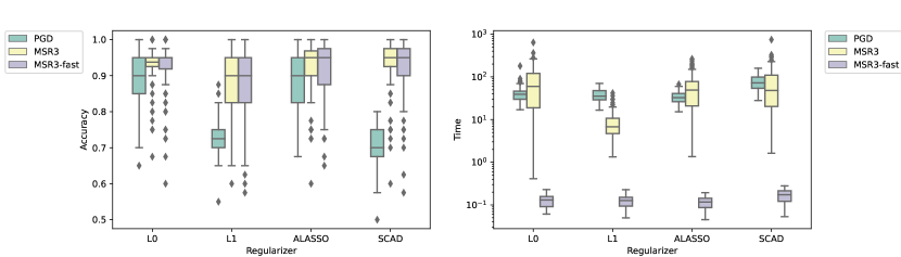
Figure 1. Feature selection accuracy and execution time in seconds for PGD and MSR3 with various regularizers. MSR3-Fast has the same accuracy as MSR3 and significantly decreases computation time.

Appendix A Existence of Minimizers (Theorems 1 and 2)

The key tool to prove existence of minimizers for both the likelihood and the penalized likelihood is the function $f:\operatorname{\mathbb{R}}^{n}\times\operatorname{\mathbb{S}}_{++}^{n}\rightarrow\operatorname{\mathbb{R}}$ given by

(39) $$\begin{split}f(r,M):=\mbox{\small$\frac{1}{2}$}[r^{T}M^{-1}r+\ln|M|]\ .\end{split}$$

If $M=U\mathrm{Diag}\left(\mu\right)U^{T}$ is the eigenvalue decomposition for $M$ where $U^{T}U=I$, and $\tilde{r}=U^{T}r$, then

(40) $$\begin{split}f(r,M)=\mbox{\small$\frac{1}{2}$}\left[\sum_{i=1}^{n}\frac{\tilde{r}_{i}^{2}}{\mu_{i}}+\ln(\mu_{i})\right].\end{split}$$

For $\rho>0$, observe that $\frac{\rho^{2}}{\omega}+\ln(\omega)$ is greater that both $\ln(\omega)$ and $1+2\ln(\rho)$ for all $\omega>0$. Therefore, using the facts $\mu_{\text{max}}(M)=\left\|M\right\|$ and $\left\|\tilde{r}\right\|_{\infty}\geq(\left\|\tilde{r}\right\|/\sqrt{n})=(\left\|r\right\|/\sqrt{n})$, we have

(41) $$\begin{split}f(r,M)&\geq\mbox{\small$\frac{1}{2}$}\sum_{i=1}^{n}\max\{\ln\mu_{i},\,1+2\ln|\tilde{r}_{i}|\}\\ &\geq\max\{1\!+\!2\ln(\left\|r\right\|/\sqrt{n})\!+\!\frac{n\!-\!1}{2}\ln\mu_{\text{min}}(M),\ \ln\left\|M\right\|\!+\!\frac{n\!-\!1}{2}\ln\mu_{\text{min}}(M)\}\\ &\geq\max\{\ln(\left\|r\right\|^{2}/n),\ln\left\|M\right\|\}+\frac{n\!-\!1}{2}\ln\mu_{\text{min}}(M),\end{split}$$

where $\mu_{\text{min}}(M)$ and $\mu_{\text{max}}(M)$ are the smallest and largest eigenvalue of $M$, respectively. We have the following result due to [33] modified slightly with an independent proof.

Lemma 16 (Level Compactness of $f$).

[33, Theorem 1] Let $f$ be as given in (39). Then, given $\rho\in\operatorname{\mathbb{R}}$ and $\alpha>0$, the set

$$\operatorname{\mathcal{D}}_{\rho,\alpha}:=\left\{(r,M)\in\operatorname{\mathbb{R}}^{n}\times\operatorname{\mathbb{S}}_{++}^{n}\,\left|\,f(r,M)\leq\rho\ \text{and}\ \mu_{\text{min}}(M)\geq\alpha\right.\right\}$$

is compact, where $\mu_{\text{min}}(M)$ and $\mu_{\text{max}}(M)$ are the smallest and largest eigenvalue of $M$, respectively.

Proof.

If $\operatorname{\mathcal{D}}_{\rho,\alpha}=\emptyset$, it is compact so we assume it is not empty. Since $f$ is continuous on $\operatorname{\mathcal{D}}_{\rho,\alpha}$, we need only show that this set is bounded. The boundedness of this set follows immediately from (41). Indeed, if $\{(r^{k},M_{k})\}\subset\operatorname{\mathbb{R}}^{n}\times\operatorname{\mathbb{S}}_{++}^{n}$ diverges in norm then, without loss of generality, either $\left\|r^{k}\right\|\rightarrow\infty$ or $\mu_{\text{max}}(M)=\left\|M_{k}\right\|\rightarrow\infty$, or both in which case (41) tells us that $f(r^{k},M_{k})\rightarrow\infty$. ∎

Observe that

$$\operatorname{\mathcal{L}}_{ML}(\beta,\Gamma)=f(r(\beta),\Omega(\Gamma))$$

where $r:\operatorname{\mathbb{R}}^{p}\rightarrow n$ and $\Omega:\operatorname{\mathbb{R}}^{q}\rightarrow\operatorname{\mathbb{S}}^{n}$ are the affine transformations

$$r(\beta) :=X\beta-Y,\qquad\text{and}$$

$$\Omega(\Gamma) :=\mathrm{Diag}\left(\Lambda_{1}+Z_{1}\Gamma Z_{1}^{T},\dots,\Lambda_{m}+Z_{m}\Gamma Z_{m}^{T}\right).$$

For $i=1,\dots,m$, define

$$\omega^{i}_{\text{min}}:=\mu_{\text{min}}(\Lambda_{i})+\mu_{\text{min}}(\Gamma)\sigma^{2}_{\text{min}}(Z_{i})\quad\mbox{ and }\quad\omega_{\text{min}}:=\min_{i=1,\dots,m}\omega^{i}_{\text{min}},$$

where $\mu_{\text{min}}(\Psi)$ and $\sigma_{\text{min}}(\Phi)$ are the smallest eigenvalues and singular-values of $\Psi$ and $\Phi$, respectively. By [1, Theorem 3.1],

(42) $$\begin{split}0<{\tilde{\alpha}}:=\mu_{\text{min}}(\Lambda)\leq\omega_{\text{min}}\leq\mu_{\text{min}}(\Omega(\Gamma))\quad\forall\ \Gamma\in\operatorname{\mathbb{S}}_{+}^{q}.\end{split}$$

Proof for Theorem 1

The bound (42) tell us that

$$\hat{\operatorname{\mathcal{D}}}:=\left\{(r,\Omega(\Gamma))\,\left|\,r\in\operatorname{\mathbb{R}}^{n},\,\Gamma\in\operatorname{\mathbb{S}}_{+}^{q}\ \text{and}\ f(r,\Omega(\Gamma))\leq\rho\right.\right\}\subset\operatorname{\mathcal{D}}_{{\tilde{\alpha}},\rho}.$$

In particular, $\operatorname{\mathcal{L}}$ is bounded below by (41). Hence there exists a sequence $\{(\beta^{k},\Gamma^{k})\}\subset\operatorname{\mathbb{R}}^{p}\times\operatorname{\mathbb{S}}_{+}^{q}$ such that

$$\operatorname{\mathcal{L}}_{ML}(\beta^{k},\Gamma_{k})\downarrow\inf_{\beta\in\operatorname{\mathbb{R}}^{p},\Gamma\in\operatorname{\mathbb{S}}_{+}^{q}}\operatorname{\mathcal{L}}_{ML}(\beta,\Gamma).$$

Let $\rho=\operatorname{\mathcal{L}}_{ML}(\beta^{0},\Gamma_{0})$. Since $f$ is continuous on $\hat{\operatorname{\mathcal{D}}}\subset\operatorname{\mathcal{D}}_{{\tilde{\alpha}},\rho}$, $\operatorname{\mathcal{D}}_{{\tilde{\alpha}},\rho}$ is compact by Lemma 16, and both ${\mathrm{Im}\left(X\right)}$ and ${\mathrm{Im}\left(\Omega\right)}$ are closed, with no loss in generality there is a $({\bar{\xi}},\overline{\Omega})\in{\mathrm{Im}\left(r\right)}\times{\mathrm{Im}\left(\Omega\right)}\cap\operatorname{\mathcal{D}}_{{\tilde{\alpha}},\rho}$ such that $(r(\beta^{k}),\Omega(\Gamma_{k}))\rightarrow({\bar{\xi}},\overline{\Omega})$. Since $({\bar{\xi}},\overline{\Omega})\in{\mathrm{Im}\left(r\right)}\times{\mathrm{Im}\left(\Omega\right)}$, there is a $({\bar{\beta}},\overline{\Gamma})\in\operatorname{\mathbb{R}}^{p}\times\operatorname{\mathbb{S}}^{q}_{+}$ such that $({\bar{\xi}},\overline{\Omega})=(r({\bar{\beta}}),\Omega(\overline{\Gamma}))$. In addition, since $0<{\tilde{\alpha}}\leq\mu_{\text{min}}(\Omega(\Gamma))$ for all $\Gamma\in\operatorname{\mathbb{S}}_{+}^{q}$, we have $\operatorname{\mathcal{L}}_{ML}$ is lsc at $({\bar{\beta}},\overline{\Gamma})$ telling us that $\operatorname{\mathcal{L}}({\bar{\beta}},\overline{\Gamma})=\inf_{\beta\in\operatorname{\mathbb{R}}^{p},\Gamma\in\operatorname{\mathbb{S}}_{+}^{q}}\operatorname{\mathcal{L}}(\beta,\Gamma)$.

Proof of Theorem 2

Define the affine transformations ${\widehat{\Omega}}:\operatorname{\mathbb{R}}^{q}\rightarrow\operatorname{\mathbb{S}}^{n}$ and ${\widehat{\Omega}}_{i}:\operatorname{\mathbb{R}}^{q}\rightarrow\operatorname{\mathbb{S}}^{n_{i}}$ by

(43) $${\widehat{\Omega}}(\gamma):=\Omega(\mathrm{Diag}\left(\gamma\right))\ \ \text{ and }\ \ {\widehat{\Omega}}_{i}(\gamma):=\Omega_{i}(\mathrm{Diag}\left(\gamma\right))\quad i=1,\dots,m.$$

The existence of a solution follows immediately once the level compactness of $\L+{\widehat{R}}$ is establinshed. To this end observe that $\operatorname{\mathcal{L}}(\beta,\gamma)=\operatorname{\mathcal{L}}_{ML}(\beta,\mathrm{Diag}\left(\gamma\right))=f(r(\beta),{\widehat{\Omega}}(\gamma))$ and so (41) and (42) tell us that $\operatorname{\mathcal{L}}(\beta,\gamma)\geq\frac{n\!+\!1}{2}\ln{\tilde{\alpha}}.$ Since ${\widehat{R}}$ is level compact, it is lower bounded. Therefore, $\operatorname{\mathcal{L}}+{\widehat{R}}$ is bounded below. Let $\rho\in\operatorname{\mathbb{R}}$ and $\{(\beta^{k},\gamma^{k})\}\subset\left\{(\beta,\gamma)\,\left|\,\operatorname{\mathcal{L}}(\beta,\gamma)+{\widehat{R}}(\beta,\gamma)\leq\rho\right.\right\}$. We need to show that $\{(\beta^{k},\gamma^{k})\}$ is bounded. If $\left\|(\beta^{k},\gamma^{k})\right\|\rightarrow\infty$, then ${\widehat{R}}(\beta^{k},\gamma^{k})\rightarrow\infty$. Since $\operatorname{\mathcal{L}}(\beta^{k},\gamma^{k})+{\widehat{R}}(\beta^{k},\gamma^{k})\leq\rho$, we must have $\operatorname{\mathcal{L}}(\beta^{k},\gamma^{k})\rightarrow-\infty$. But $\operatorname{\mathcal{L}}$ is bounded below, hence $\{(\beta^{k},\gamma^{k})\}$must be bounded, and so $\operatorname{\mathcal{L}}+{\widehat{R}}$ is level compact.

Appendix B Derivatives of $\operatorname{\mathcal{L}}$

One can show that

(44) $$\begin{split}\nabla_{\beta}\operatorname{\mathcal{L}}(\beta,\gamma)&=\sum_{i=1}^{m}X_{i}^{T}\Omega_{i}^{-1}(X_{i}\beta-Y_{i})=X^{T}\Omega^{-1}r(\beta)\\ \nabla_{\gamma}\operatorname{\mathcal{L}}(\beta,\gamma)&=\mbox{\small$\frac{1}{2}$}\sum_{i=1}^{m}\mathrm{diag}\left({Z_{i}}^{T}\Omega_{i}^{-1}Z_{i}\right)-({Z_{i}}^{T}\Omega_{i}^{-1}(X_{i}\beta-Y_{i}))^{\circ 2}\\ \nabla_{\beta\beta}\operatorname{\mathcal{L}}(\beta,\gamma)&=\sum_{i=1}^{m}X_{i}^{T}\Omega_{i}^{-1}X_{i}=X^{T}\Omega^{-1}X\\ \nabla_{\beta\gamma}\operatorname{\mathcal{L}}(\beta,\gamma)&=-\sum_{i=1}^{m}\mathrm{Diag}\left(Z_{i}^{T}\Omega_{i}^{-1}(X_{i}\beta-Y_{i})\right)Z_{i}^{T}\Omega_{i}^{-1}X_{i}\\ \nabla_{\gamma\gamma}\operatorname{\mathcal{L}}(\beta,\gamma)&\!=\!\!\sum_{i=1}^{m}\!\left(Z_{i}^{T}\Omega_{i}^{-1}(X_{i}\beta\!-\!Y_{i})(X_{i}\beta\!-\!Y_{i})^{T}\Omega_{i}^{-1}Z_{i}\right)\!\circ\!(Z_{i}^{T}\Omega_{i}^{-1}Z_{i})\!-\!\mbox{\small$\mbox{\small$\frac{1}{2}$}$}(Z_{i}^{T}\Omega_{i}^{-1}Z_{i})^{\circ 2},\end{split}$$

where the final representation can be rewritten using the fact that $(yz^{T})\circ A=\mathrm{Diag}\left(y\right)A\mathrm{Diag}\left(z\right)$ for all $y\in\operatorname{\mathbb{R}}^{m},z\in\operatorname{\mathbb{R}}^{n},\ A\in\operatorname{\mathbb{R}}^{m\times n}$ [14]. These formulas imply that

(45) $$\nabla^{2}\operatorname{\mathcal{L}}{(\beta,\gamma)}=\sum_{i=1}^{m}S_{i}^{T}\begin{bmatrix}X_{i}^{T}\\ -Z_{i}^{T}\end{bmatrix}\Omega_{i}(\gamma)^{-1}\begin{bmatrix}X_{i}^{T}&-Z_{i}^{T}\end{bmatrix}S_{i}-\begin{bmatrix}0&0\\ 0&\mbox{\small$\frac{1}{2}$}(Z_{i}^{T}\Omega_{i}(\gamma)^{-1}Z_{i})^{\circ 2}\end{bmatrix},$$

where

$$S_{i}:=\begin{bmatrix}I_{q}&0\\ 0&\mathrm{Diag}\left(Z_{i}^{T}\Omega_{i}(\gamma)^{-1}(X_{i}\beta-Y_{i})\right)\end{bmatrix}.$$

These formulas are also derived in [19].

References

• [1] A. Aravkin, J.V. Burke, B. Bell, and G. Pillonetto. Algorithms for block tridiagonal systems: Foundations and new results for generalized kalman smoothing. To appear in 19th IFAC Symposium on System Identification (SYSID 2021), 2021.
• [2] A.Y. Aravkin, J.V. Burke, D. Drusvyatskyi, M.P. Friedlander, and K.J. Macphee. Foundations of gauge and perspective duality. SIAM J. on Opt., 28:2406 – 2434, 2018.
• [3] A.Y. Aravkin, J.V. Burke, and M.P. Friedlander. Variational properties of value functions. SIAM J. on Opt., 23:1689 – 1717, 2013.
• [4] Amir Beck. First-Order Methods in Optimization. MOS-SIAM Series on Optimization. SIAM, 2017.
• [5] Howard D. Bondell, Arun Krishna, and Sujit K. Ghosh. Joint Variable Selection for Fixed and Random Effects in Linear Mixed-Effects Models. Biometrics, 66(4):1069–1077, dec 2010.
• [6] J.V. Burke and A. Engle. Line search and trust-region methods for convex-composite optimization. arXiv:1806.05218, 2018.
• [7] Simona Buscemi and Antonella Plaia. Model selection in linear mixed-effect models. AStA Advances in Statistical Analysis, 2019.
• [8] Fei Chen, Zaixing Li, Lei Shi, and Lixing Zhu. Inference for mixed models of anova type with high-dimensional data. Journal of Multivariate Analysis, 133:382–401, 2015.
• [9] Rebecca DerSimonian and Nan Laird. Meta-analysis in clinical trials. Controlled clinical trials, 7(3):177–188, 1986.
• [10] Yali Fan, Guoyou Qin, and Zhong Yi Zhu. Robust variable selection in linear mixed models. Communications in Statistics-Theory and Methods, 43(21):4566–4581, 2014.
• [11] Yingying Fan and Runze Li. Variable selection in linear mixed effects models. The Annals of Statistics, 40(4):2043–2068, aug 2012.
• [12] Jerome Friedman, Trevor Hastie, and Robert Tibshirani. Regularization paths for generalized linear models via coordinate descent. Journal of Statistical Software, 33(1):1–22, 2010.
• [13] Abhik Ghosh and Magne Thoresen. Non-concave penalization in linear mixed-effect models and regularized selection of fixed effects. AStA Advances in Statistical Analysis, 102(2):179–210, 2018.
• [14] R.A. Horn and C.R. Johnson. Matrix Analysis. Cambridge University Press, 1985.
• [15] Joseph G Ibrahim, Hongtu Zhu, Ramon I Garcia, and Ruixin Guo. Fixed and random effects selection in mixed effects models. Biometrics, 67(2):495–503, 2011.
• [16] Joseph G. Ibrahim, Hongtu Zhu, Ramon I. Garcia, and Ruixin Guo. Fixed and Random Effects Selection in Mixed Effects Models. Biometrics, 67(2):495–503, jun 2011.
• [17] Lan Lan. Variable Selection in Linear Mixed Model for Longitudinal Data. PhD thesis, 2006.
• [18] Bingqing Lin, Zhen Pang, and Jiming Jiang. Fixed and random effects selection by REML and pathwise coordinate optimization. Journal of Computational and Graphical Statistics, 22(2):341–355, 2013.
• [19] Mary J. Lindstrom and Douglas M. Bates. Newton-Raphson and EM Algorithms for Linear Mixed-Effects Models for Repeated-Measures Data. Journal of the American Statistical Association, 83(404):1014, dec 1988.
• [20] T.-T. Lu and S.-H. Shiou. Inverses of $2\times 2$ block matrices. Computers and Mathematics with Applications, 43:119–129, 2002.
• [21] Christopher JL Murray, Aleksandr Y Aravkin, Peng Zheng, Cristiana Abbafati, Kaja M Abbas, Mohsen Abbasi-Kangevari, Foad Abd-Allah, Ahmed Abdelalim, Mohammad Abdollahi, Ibrahim Abdollahpour, et al. Global burden of 87 risk factors in 204 countries and territories, 1990–2019: a systematic analysis for the global burden of disease study 2019. The Lancet, 396(10258):1223–1249, 2020.
• [22] Juming Pan and Junfeng Shang. A simultaneous variable selection methodology for linear mixed models. Journal of Statistical Computation and Simulation, 88(17):3323–3337, 2018.
• [23] H. D. Patterson and R. Thompson. Recovery of Inter-Block Information when Block Sizes are Unequal. Biometrika, 58(3):545, dec 1971.
• [24] José C. Pinheiro and Douglas M. Bates. Mixed-Effects Models in Sand S-PLUS. Journal of the American Statistical Association, 96(455):1135–1136, sep 2000.
• [25] Robert C. Reiner, Ryan M. Barber, James K. Collins, Peng Zheng, Simon I. Hay, Stephen S. Lim, Christopher J. L. Murray, and IHME COVID-19 Forecasting Team. Modeling covid-19 scenarios for the United States. Nature medicine, 2020.
• [26] R Tyrrell Rockafellar and Roger J-B Wets. Variational analysis, volume 317. Springer Science & Business Media, 2009.
• [27] A. Sholokhov, J.V. Burke, D.F. Santomauro, P. Zheng, and A. Aravkin. A relaxation approach to feature selection for linear mixed effects models. In Preparation, 2022.
• [28] Robert Tibshirani. Regression shrinkage and selection via the lasso. Journal of the Royal Statistical Society: Series B (Methodological), 58(1):267–288, 1996.
• [29] Florin Vaida and Suzette Blanchard. Conditional Akaike information for mixed-effects models. Biometrika, 92(2):351–370, jun 2005.
• [30] Stephen J. Wright. Primal-Dual Interior-Point Methods. SIAM, 1997.
• [31] Peirong Xu, Tao Wang, Hongtu Zhu, and Lixing Zhu. Double Penalized H-Likelihood for Selection of Fixed and Random Effects in Mixed Effects Models. Statistics in Biosciences, 7(1):108–128, 2015.
• [32] Peng Zheng, Travis Askham, Steven L. Brunton, J. Nathan Kutz, and Aleksandr Y. Aravkin. A Unified Framework for Sparse Relaxed Regularized Regression: SR3. IEEE Access, 7:1404–1423, 2019.
• [33] Peng Zheng, Ryan Barber, Reed JD Sorensen, Christopher JL Murray, and Aleksandr Y Aravkin. Trimmed constrained mixed effects models: formulations and algorithms. Journal of Computational and Graphical Statistics, pages 1–13, 2021.
• [34] Alain Zuur, Elena N Ieno, Neil Walker, Anatoly A Saveliev, and Graham M Smith. Mixed effects models and extensions in ecology with R. Springer Science & Business Media, 2009.