Constraining modifications of black hole perturbation potentials near the light ring with quasinormal modes

Abstract

In modified theories of gravity, the potentials appearing in the Schrödinger-like equations that describe perturbations of non-rotating black holes are also modified. In this paper we ask: can these modifications be constrained with high-precision gravitational-wave measurements of the black hole’s quasinormal mode frequencies? We expand the modifications in a small perturbative parameter regulating the deviation from the general-relativistic potential, and in powers of $M/r$. We compute the quasinormal modes of the modified potential up to quadratic order in the perturbative parameter. Then we use Markov-chain-Monte-Carlo (MCMC) methods to recover the coefficients in the $M/r$ expansion in an “optimistic” scenario where we vary them one at a time, and in a “pessimistic” scenario where we vary them all simultaneously. In both cases, we find that the bounds on the individual parameters are not robust. Because quasinormal mode frequencies are related to the behavior of the perturbation potential near the light ring, we propose a different strategy. Inspired by Wentzel–Kramers–Brillouin (WKB) theory, we demonstrate that the value of the potential and of its second derivative at the light ring can be robustly constrained. These constraints allow for a more direct comparison between tests based on black hole spectroscopy and observations of black hole “shadows” by the Event Horizon Telescope and future instruments.

I Introduction

Since the first groundbreaking direct detection of gravitational waves in 2015 Abbott et al. (2016a), the LIGO-Virgo-KAGRA collaboration has reported around one hundred additional events Abbott et al. (2019a, 2021a, 2021b); Nitz et al. (2021); Olsen et al. (2022). Most of the detected signals are in agreement with the predictions of general relativity (GR) for the merger of two black holes, while some of them involve neutron stars. Besides the important implications for astrophysical formation scenarios of black hole populations, these events allow for unprecedented tests of GR in the strong field Berti et al. (2015); Barack et al. (2019); Yunes et al. (2016); Cardoso and Gualtieri (2016); Berti et al. (2018a, b); Cardoso and Pani (2019); Abbott et al. (2016b, 2019b, 2021c, 2021d); Ghosh et al. (2021). A key prediction from GR is that rotating astrophysical black holes should be described by the Kerr metric, and that their perturbative dynamics at late times (in the so-called “ringdown” regime) should be well described by a superposition of damped sinusoids called quasinormal modes (QNMs), with characteristic frequencies determined only by the black hole’s mass and spin. If GR is the correct theory of gravity, the observed QNM frequencies should match those predicted in GR for Kerr black holes Detweiler (1980); Dreyer et al. (2004); Berti et al. (2006).

The LIGO-Virgo-KAGRA collaboration has analyzed the current catalogs, at first focusing on GW150914 and then using multiple events, with the specific aim to extract QNMs from the ringdown Abbott et al. (2016b, 2019b, 2021c, 2021d). The observations are generally consistent with the presence of the quadrupole ($\ell=m=2$) fundamental mode (with “overtone number” $n=0$). Reference Isi et al. (2019) claimed evidence for the presence of overtones (higher-damping $\ell=m=2$ modes with $n>0$) in GW150914, and Ref. Capano et al. (2021) claimed evidence for the fundamental mode with $\ell=m=3$ in GW190521. Later work showed that these conclusions depend on the detector noise, data analysis methods, the choice of starting time, and nonlinear effects in the theoretical modeling of ringdown Cotesta et al. (2022); Finch and Moore (2022); Isi and Farr (2022); Capano et al. (2022); Sberna et al. (2022); Cheung et al. (2022); Mitman et al. (2022). Despite the ongoing debate, the analysis of numerical relativity simulations implies that at least some overtones can in principle be extracted when the signal-to-noise ratio is large enough Berti et al. (2007); Baibhav et al. (2018); Giesler et al. (2019); Ota and Chirenti (2020); Bhagwat et al. (2020a, b); Cook (2020); Bustillo et al. (2021); Jiménez Forteza et al. (2020); Magaña Zertuche et al. (2022). Theoretical modeling and data analysis challenges may be more subtle than anticipated, but next-generation detectors are expected to provide reliable, high-precision measurements of more than one QNM Berti et al. (2016); Cabero et al. (2020); Ota and Chirenti (2022); Bhagwat et al. (2022). Therefore it is important to investigate how these measurements will inform us on possible deviations from GR.

There have been various attempts to introduce deviations from GR in the QNM spectrum in a theory-agnostic manner. These include modifications of the gravitational action around a GR black hole background Tattersall et al. (2018), the addition of perturbative corrections at the level of the perturbation equations Cardoso et al. (2019); McManus et al. (2019); Völkel et al. (2022) or at the level of the metric Völkel and Barausse (2020); Konoplya and Zhidenko (2022) (which then require suitable assumptions for the dynamics), or the addition of free parameters in the QNM frequencies themselves Meidam et al. (2014); Maselli et al. (2020); Carullo (2021). While the physical interpretation of these “theory-agnostic” constraints requires a specific modified theory of gravity, it is desirable to have a robust phenomenological framework encompassing several theories and allowing us to solve the “inverse problem” – i.e., to infer what specific GR modification caused a deviation from GR.

For non-rotating spacetimes, the inverse problem based on parametrized black hole metrics for axial (odd parity) perturbations was studied in Ref. Völkel and Barausse (2020). For spinning black holes, a parametrized spectroscopy framework (“ParSpec”) was introduced in Ref. Maselli et al. (2020), and applied to data in Ref. Carullo (2021). The ParSpec framework is based on a Taylor-series expansion of the QNM frequencies in the dimensionless Kerr spin parameter. In principle this can be used to stack multiple events Yang et al. (2017), and then compare with the predictions from specific theories.

In this work we assume that deviations from the QNM spectrum in GR can be adequately captured by small modifications of the underlying perturbation equations. As a proof of principle, we focus on non-rotating or slowly rotating black holes. We adopt the parametrized formalism of Refs. Cardoso et al. (2019); McManus et al. (2019), which systematically connects small deviations in the perturbation equations with the QNM spectrum. At lowest order, the idea is to consider small modifications in the perturbation potential at the linear level and to write them as a “post-Newtonian” (PN) series expansion in $M/r$ Cardoso et al. (2019). Going to quadratic order allows one to capture (more realistically) possible couplings to additional fields McManus et al. (2019). While in Refs. Cardoso et al. (2019); McManus et al. (2019) the focus is on the fundamental mode, Ref. Völkel et al. (2022) extended the analysis to overtones, and studied the inverse problem using a principal component analysis.

We apply a Bayesian analysis to solve the inverse problem: given a simulated set of QNM frequencies computed within the parametrized formalism, can we infer the deviation parameters in the underlying potentials? We are particularly interested in the understanding whether it is possible to constrain the more general and realistic case where many deviation parameters are varied simultaneously. Therefore we compute constraints on the individual PN-like expansion parameters twice: we first vary the parameters one at a time (“optimistic” case), and then we vary them all simultaneously (“pessimistic” case). In both cases we find that the constraints on the individual expansion parameters are not robust. The priors play an important role, especially when all parameters are varied simultaneously. In particular in the “optimistic” case the recovered bounds on the individual parameters can be biased.

However, the complex correlations in the posterior distributions in the “pessimistic” case contain valuable information. It has long been known that QNM frequencies are related to the behavior of the perturbation potential near the light ring Press (1971); Schutz and Will (1985); Cardoso et al. (2009). Therefore we propose a different strategy: we map the PN series expansion to the value of the potential and its derivatives at the peak by using insights from Wentzel–Kramers–Brillouin (WKB) theory. Higher-order WKB methods relate the QNM frequencies with a Taylor expansion of the effective perturbation potential in the vicinity of its maximum, i.e., close to the light-ring Schutz and Will (1985); Iyer and Will (1987); Konoplya (2003); Matyjasek and Opala (2017). In fact, the (closely related) eikonal approximation was used in Refs. Glampedakis et al. (2017); Glampedakis and Silva (2019); Silva and Glampedakis (2020); Bryant et al. (2021) to build a “post-Kerr” strategy to parametrized black hole spectroscopy. By connecting the Taylor (PN-like) expansion to the light-ring WKB expansion, we demonstrate that the value of the potential and of its second derivative at the light ring can be robustly constrained using Bayesian techniques.

Our work suggests that it may be possible to relate black hole spectroscopy tests to electromagnetic observations of black hole “shadows” by the Event Horizon Telescope and future instruments Akiyama et al. (2019a, b); Völkel et al. (2021); Kocherlakota et al. (2021). However, the interpretation of parametrized QNM tests of strong-field gravity will require very precise measurements and a more solid theoretical understanding of QNM excitation.

The paper is structured as follows. In Sec. II we introduce our theoretical framework and Bayesian data analysis techniques. In Sec. III we apply the method to GR and non-GR injections. In Sec. IV we discuss our results and outline possible directions for future work. Throughout the paper we adopt geometrical units ($G=c=1$).

II Methodology

In this section we give an overview of the three main ingredients of our method: the parametrized QNM framework based on a Taylor expansion of the perturbation to the GR potential (Sec. II.1), the WKB expansion of the modified potential near the light right (Sec. II.2), and the Bayesian inference approach used to address the inverse problem (Sec. II.3).

II.1 Parametrized QNM framework

The perturbations of the Schwarzschild black hole were first studied in the odd-parity (axial) case by Regge and Wheeler Regge and Wheeler (1957), and later extended to the even-parity (polar) case by Zerilli Zerilli (1970). The more general case of Kerr black holes was worked out by Teukolsky Teukolsky (1973).

The characteristic frequencies and damping times of the QNMs for rotating and non-rotating black holes in GR have long been known (see Kokkotas and Schmidt (1999); Nollert (1999); Berti et al. (2009); Konoplya and Zhidenko (2011); Pani (2013) for reviews). More recently, various authors have considered black hole perturbations and QNMs in modified theories of gravity. Almost all works are limited to non-rotating or slowly rotating black holes Cardoso and Gualtieri (2009); Molina et al. (2010); Blázquez-Salcedo et al. (2016, 2017, 2020a, 2020b); Franchini et al. (2021), because finding exact analytical background solutions for arbitrary rotation is not always possible, and separating the perturbation equations is even harder (if at all possible). Theory-specific works using the slow-rotation approximation for gravitational perturbations include dynamical Chern-Simons gravity Wagle et al. (2022); Srivastava et al. (2021), Einstein-dilaton-Gauss-Bonnet gravity Pierini and Gualtieri (2021, 2022), and effective-field-theory extensions of GR including higher-derivative terms Cano et al. (2020, 2022), although there are recent attempts at formulating generalized Teukolsky equations valid for more generic theories and arbitrary rotation Li et al. (2022); Hussain and Zimmerman (2022).

Since Einstein’s theory is very well tested in the weak- and strong-field regimes, from an experimental point of view it is reasonable to treat possible modifications as small deviations from GR. Under this assumption, the parametrized framework developed in Refs. Cardoso et al. (2019); McManus et al. (2019); Völkel et al. (2022) allows for a convenient and efficient calculation of QNMs once the perturbation equations are cast in the form

$$\frac{\mathrm{d}^{2}{\Phi}}{\mathrm{d}r_{*}^{2}}+\left[\omega^{2}-V(r)\right]{\Phi}=0\,,$$ (1)

where the radial function $\Phi$ comes from a spherical harmonic decomposition of the perturbed metric or of some other perturbing field, the tortoise coordinate $r_{*}$ is defined in terms of the areal radius $r$ and the function $f=1-r_{\mathrm{H}}/r$ through $\mathrm{d}r_{*}=\mathrm{d}r/f$, where $r_{\mathrm{H}}$ is the location of the black horizon, and $\omega$ is the complex QNM frequency. For metric perturbations we can write

$$V(r) =V_{\text{\tiny{GR}}}(r)+\sum_{k=0}^{\infty}\alpha^{(k)}\delta V_{k}(r)\,,$$ (2)

where $V_{\text{\tiny{GR}}}$ is either the Regge-Wheeler or Zerilli potential, and

$$\delta V_{k}(r)=\frac{f(r)}{r_{\mathrm{H}}^{2}}\left(\frac{r_{\mathrm{H}}}{r}\right)^{k}\,.$$ (3)

If the coefficients $\alpha^{(k)}$ are small, the QNMs obtained by the solution of Eq. (1) can be approximated, up to second order, by the expression

$$\omega\approx\omega^{0}+\alpha^{(k)}d_{(k)}+\frac{1}{2}\alpha^{(k)}\alpha^{(s)}e_{(ks)}\,,$$ (4)

where $\omega^{0}$ are the GR frequencies, and the coefficients $d_{(k)}$ and $e_{(ks)}$ were first introduced in Cardoso et al. (2019); McManus et al. (2019). We compute these coefficients via a continued-fraction method, as in Ref. Völkel et al. (2022). Note that in general the $\alpha^{(k)}$ can be complex numbers and might depend on the unperturbed QNM frequency, and thus also on the overtone number itself. We are also neglecting a quadratic correction term proportional to the possible QNM dependence of the potential correction term, which can be found in Ref. McManus et al. (2019). By a redefinition of the field it is possible to reduce the number of parameters in the potential Kimura (2020), but this was only demonstrated in the linear case, and it might not be possible in the quadratic case studied in this work (or in the more general and realistic case of rotating black holes).

The $\alpha^{(k)}$ coefficients must be small enough for the QNM frequencies to be adequately approximated by a quadratic expansion in $\alpha^{(k)}$. Therefore we impose the following – necessary but not sufficient – “convergence criterion” (see Cardoso et al. (2019)):

$$\alpha^{(k)}\ll\alpha^{(k)}_{\text{\tiny{M}}}\equiv(k+1)\left(1+\frac{1}{k}\right)^{k}.$$ (5)

II.2 Higher-order WKB method

The QNMs in this work are obtained either numerically (with a continued fraction method) or analytically (through the parametrized QNM framework). However, it will be useful to analyze our results by making use of the physical insight derived from a higher-order WKB approximation. The WKB approximation is widely used for scattering problems of the form of Eq. (1), if the potential describes a barrier with a single maximum and suitable asymptotics. Within black hole perturbation theory, the leading-order WKB approximation is known as the Schutz-Will formula Schutz and Will (1985), and it was later generalized to higher orders Iyer and Will (1987); Konoplya (2003); Matyjasek and Opala (2017). The higher-order WKB approximation can be written, schematically, as

$$\omega_{n}^{2}=V^{(0)}-\mathrm{i}\sqrt{-2V^{(2)}}\left(n+\frac{1}{2}\right)+\sum_{i}{\tilde{\Lambda}_{i}(n)}\,,$$ (6)

where $n$ is the overtone number. The correction terms in the WKB approximation $\tilde{\Lambda}_{i}(n)$ are lengthy expressions Iyer and Will (1987); Konoplya (2003); Matyjasek and Opala (2017) (for completeness, we list them in Appendix A up to third order). They involve derivatives $V^{(p)}$ of the effective potential with respect to the tortoise coordinate, evaluated at the maximum of the potential:

$$V^{(p)}=\frac{\mathrm{d}^{p}V}{\mathrm{d}r_{*}^{p}}\Bigg{|}_{r_{\text{\tiny{MAX}}}}.$$ (7)

Increasing the order of the WKB correction introduces even higher-order derivatives of the potential. In general the WKB approximation works rather well for the fundamental mode, and it becomes less accurate as $n$ increases Konoplya et al. (2019).

In the following we revise the calculation of the potential derivatives assuming a perturbative expansion in the coefficients $\alpha^{(k)}$. The maximum of $V$ with respect to the tortoise coordinate is found by solving $\mathrm{d}V/\mathrm{d}r_{*}=0$, and it is located at $r_{\text{\tiny{MAX}}}=\bar{r}+\sum_{k}\alpha^{(k)}\delta r_{k}$, where $\bar{r}$ is the location of the peak in GR and

$$\delta r_{k}=-\frac{\delta V_{k}}{V^{(2)}_{\text{\tiny{GR}}}}\Bigg{|}_{r=\bar{r}}\,.$$ (8)

At first order in $\alpha^{(k)}$, denoting with a $p$ superscript the $p$-th derivative with respect to $r_{*}$ evaluated at $r_{\text{\tiny{MAX}}}$, we have

$$V^{(p)}=V^{(p)}_{\text{\tiny{GR}}}+\sum_{k=0}^{\infty}\alpha^{(k)}\delta V^{(p)}_{k}.$$ (9)

In Fig. 1 we plot $\delta V^{(p)}_{k}$ for the $\ell=2$ axial potential (up to $p=4$) as a function of $k$ for $k\leq 40$, while in Table 1 we list the value of these derivatives for $k\leq 10$.

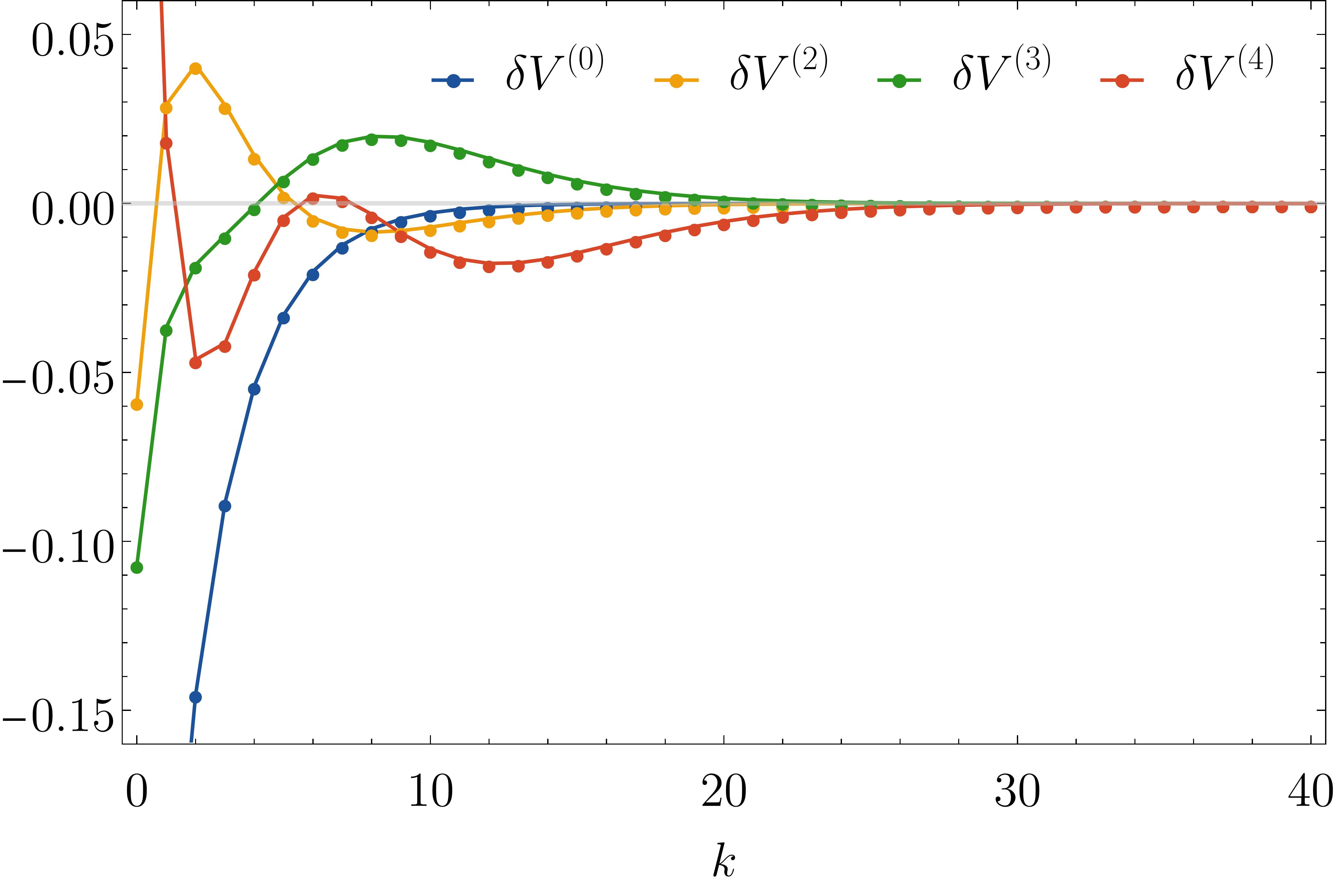
Figure 1: Displacement of the derivatives of the effective potential evaluated at the peak for different values of $k$ for axial perturbations with $\ell=2$.

$$\begin{array}[]{c|rrrr}k&\delta V^{(0)}_{k}&\delta V^{(2)}_{k}&\delta V^{(3)}_{k}&\delta V^{(4)}_{k}\\[2.15277pt] \hline\cr 0&-0.390&-0.0585&-0.107&0.256\\ 1&-0.238&0.0293&-0.0366&0.0189\\ 2&-0.145&0.0410&-0.0181&-0.0462\\ 3&-0.0884&0.0291&-0.00937&-0.0413\\ 4&-0.0539&0.0141&-0.000874&-0.0202\\ 5&-0.0329&0.00268&0.00741&-0.00407\\ 6&-0.0200&-0.00425&0.0140&0.00245\\ 7&-0.0122&-0.00756&0.0182&0.00154\\ 8&-0.00745&-0.00848&0.0199&-0.00319\\ 9&-0.00454&-0.00804&0.0196&-0.00878\\ 10&-0.00277&-0.00697&0.0181&-0.0134\\ \end{array}$$

Table 1: Derivatives of the effective potential evaluated at the peak for axial perturbations with $\ell=2$ and $k\leq 10$.

We can solve for $\omega$ and expand the result at first order in the $\alpha^{(k)}$. This yields the following relation for the frequency at third order in the WKB approximation:

$$\begin{split}\omega\approx\omega_{\text{\tiny{WKB}}}+\sum_{k=2}^{\infty}\frac{\alpha^{(k)}}{2\omega_{\text{\tiny{WKB}}}}\bigg{[}&\delta V^{(0)}_{k}+\delta V^{(2)}_{k}\frac{\omega_{\text{\tiny{WKB}}}^{2}-V^{(0)}_{\text{\tiny{GR}}}}{2V^{(2)}_{\text{\tiny{GR}}}}\\ &+\delta\tilde{\Lambda}_{2}^{k}+\delta\tilde{\Lambda}_{3}^{k}\bigg{]}\,,\end{split}$$ (10)

where $\omega_{\text{\tiny{WKB}}}$ is the frequency evaluated with the WKB method within GR, and $\delta\tilde{\Lambda}_{i}$ are the linear expansions in $\alpha$ of the coefficients $\tilde{\Lambda}_{i}$. By comparing Eqs. (4) and (10) order by order, we can map the coefficients $d_{(k)}$ to the derivatives $\delta V^{(p)}_{k}$ of the displaced potential at the peak.

II.3 Bayesian approach

Bayesian analysis allows us to relate the observed data $D$ with the underlying parameters $\theta$ of a model, or to compare different models with each other. It also allows us to quantitatively include our prior knowledge or assumptions into the analysis, and understand how they affect the posterior through Bayes’ theorem

$$\mathcal{P}\left(\theta|D\right)=\frac{\mathcal{P}\left(D|\theta\right)\mathcal{P}\left(\theta\right)}{\mathcal{P}\left(D\right)},$$ (11)

which states that the posterior $\mathcal{P}\left(\theta|D\right)$ is equal to the prior $\mathcal{P}\left(\theta\right)$ times the likelihood $\mathcal{P}\left(D|\theta\right)$, divided by the evidence $\mathcal{P}\left(D\right)$. The evidence is often unknown or hard to compute, but it is still possible to compute the posterior via Markov-chain-Monte-Carlo (MCMC) techniques. These only require the knowledge of the prior and likelihood, and can be used to directly draw samples from the posterior. Standard MCMC techniques become very computationally expensive when the number of sampled parameters is large. The parametrized QNM framework of Eq. (4) is very beneficial in this sense, because it speeds up the calculation of the likelihood significantly by avoiding the more involved (and not necessarily always converging) calculations that are necessary in other techniques. This results in quick MCMC sampling, allowing us to study a reasonable number of parameters.

We assume that our likelihood for the unknown parameters $\theta=[r_{\mathrm{H}},\alpha^{(k)}]$ is given by

$$\mathcal{P}(D|\theta)\propto\exp\left[-\frac{1}{2}\vec{h}(\theta)\mathbf{C}^{-1}\vec{h}(\theta)\right],$$ (12)

where $\mathbf{C}^{-1}$ is the inverse of the covariance matrix $\mathbf{C}$ of the QNM frequencies, and

$$\vec{h}(\theta)=\frac{r_{\mathrm{H}}^{0}}{r_{\mathrm{H}}}\vec{\omega}\left(\alpha^{(k)}\right)-\vec{D}\,,$$ (13)

where $r_{\mathrm{H}}^{0}$ is the location of the horizon as it would be inferred in GR. We perform this rescaling since we do not know a priori the correct value for $r_{\mathrm{H}}$.

The exact form of the correlations depends on the details of the observed binary black hole system, as well as the details of the detector. However, by identifying the inverse of the covariance matrix with the Fisher matrix, it is possible to use analytic estimates derived in Ref. Berti et al. (2006) as an approximation. For measurements of the fundamental QNM and of the first overtone ($n=0,1$) the Fisher matrix we need to estimate is a $4\times 4$ matrix. The submatrix that connects the real and imaginary parts of the frequency for a fixed value of $n$ can be approximated with the results of Ref. Berti et al. (2006), but the correlations between different $n$’s (i.e., the $2\times 2$ off-diagonal blocks) cannot, and therefore we neglect them. However, we have analyzed how moderate random correlations between the fundamental mode and the first overtone would change the results, and we did not find substantial qualitative changes. We rescale the Fisher matrix so that the real part of the $n=0$ mode is measured with a relative error of $1\,\%$, which yields a relative error of $4.7\,\%$ for its imaginary part. Assuming that the $n=1$ overtone is excited with a similar amplitude (an assumption justified by fits to numerical relativity simulations Giesler et al. (2019)) yields relative errors of $3.4\,\%$ and $8.2\,\%$ for the real and imaginary part of the overtone frequency, respectively. Ongoing work in the literature suggests that the specific model used to extract overtones can have an important impact on interpreting the constraints Cheung et al. (2022); Mitman et al. (2022), but this approximate estimate of the Fisher matrix is sufficient for our purposes.

The location of the black hole horizon $r_{\mathrm{H}}$ affects the QNM spectrum and depends on the underlying theory. We assume that $r_{\mathrm{H}}$ is close to its GR value $r_{\mathrm{H}}^{0}$ and that the uncertainty on $r_{\mathrm{H}}$ is relatively small ($\sigma_{r_{\mathrm{H}}}=5\,\%$), for example because we have a good estimate of the remnant black hole’s mass from the inspiral/merger waveform. Then we multiply the likelihood of Eq. (12) by an additional factor

$$\mathcal{P}_{r_{\mathrm{H}}}\equiv\exp\left[-\frac{1}{2}\left(\frac{r_{\mathrm{H}}-r_{\mathrm{H}}^{0}}{\sigma_{r_{\mathrm{H}}}}\right)^{2}\right].$$ (14)

This is equivalent to assuming a Gaussian prior for $r_{\mathrm{H}}$ centered around its value $r_{\mathrm{H}}^{0}$ in GR.

The priors $\mathcal{P}(\alpha^{(k)})$ cannot be chosen to be arbitrary because we are using a parametrized QNM framework. For the perturbative formalism to be valid, we must adopt bounds consistent with Eq. (5). For concreteness, in our analysis we consider two different prior realizations: $\alpha^{(k)}_{\text{\tiny{P20}}}\equiv\alpha^{(k)}_{\text{\tiny{M}}}/20$ and $\alpha^{(k)}_{\text{\tiny{P10}}}\equiv\alpha^{(k)}_{\text{\tiny{M}}}/10$, with $k\in[0,10]$. Our choice to study 11 parameters for $\alpha^{(k)}$ guarantees that we can explore a large parameter space to capture modifications to GR, but at the same time we can still perform efficient MCMC sampling. To perform the MCMC analysis we use the emcee sampler Foreman-Mackey et al. (2013), which is based on the affine-invariant ensemble sampler proposed by Goodman and Weare Goodman and Weare (2010). Since one would not generically expect that very large $k$ contribute in a dominant way, neglecting higher orders is a reasonable choice. Throughout this work we assume flat (uniform) priors within these two different bounds. Considering different ranges allows us to quantify what aspects of the analysis are sensitive to the choice of priors and which are not. By using the continued-fraction numerical code discussed in Ref. Völkel et al. (2022), we have checked that the frequencies generated by taking $\alpha^{(k)}=\pm\alpha^{(k)}_{\text{\tiny{P20}}}$, with $k\in[0,10]$, are well approximated by the quadratic expansion. However, for certain combinations of random draws from the larger prior range $\alpha^{(k)}=\pm\alpha^{(k)}_{\text{\tiny{P10}}}$ the approximation can become inaccurate. Our results below (based on the exact injection) show that this only mildly affects our reconstruction of the perturbative parameters that were used in the parametrized framework for the inference.

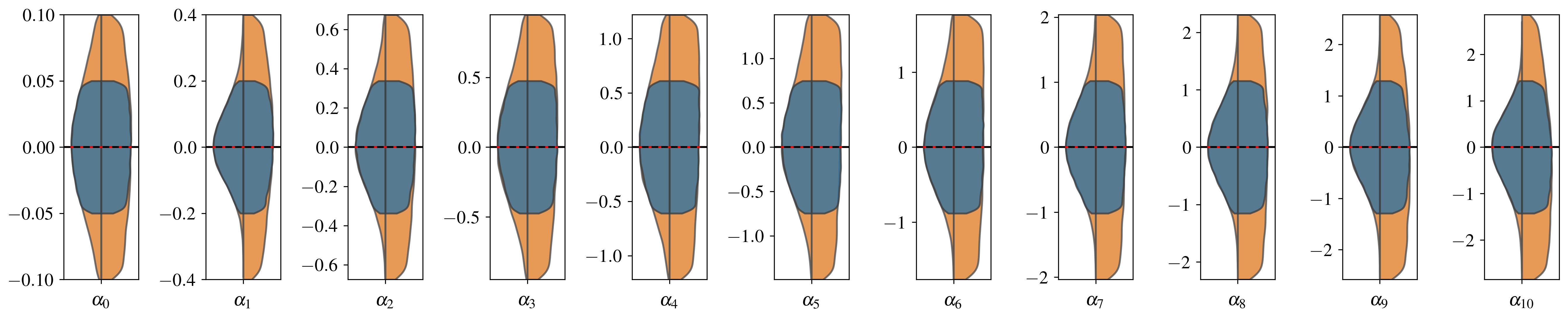
Figure 2: MCMC results for simulated observations of the Schwarzschild $n=0,1$ QNMs with relative errors described in the main text, and assuming a Gaussian prior for $r_{\mathrm{H}}$ corresponding to $5\,\%$ at $1\sigma$ confidence. In each panel, on the left side we plot the posteriors in the optimistic case (only one $\alpha^{(k)}$ is varied at a time), and on the right side we plot the posteriors in the pessimistic case (all $\alpha^{(k)}$’s are varied simultaneously). The blue (orange) color corresponds to a prior range of $\alpha^{(k)}_{\text{\tiny{P20}}}$ ($\alpha^{(k)}_{\text{\tiny{P10}}}$).

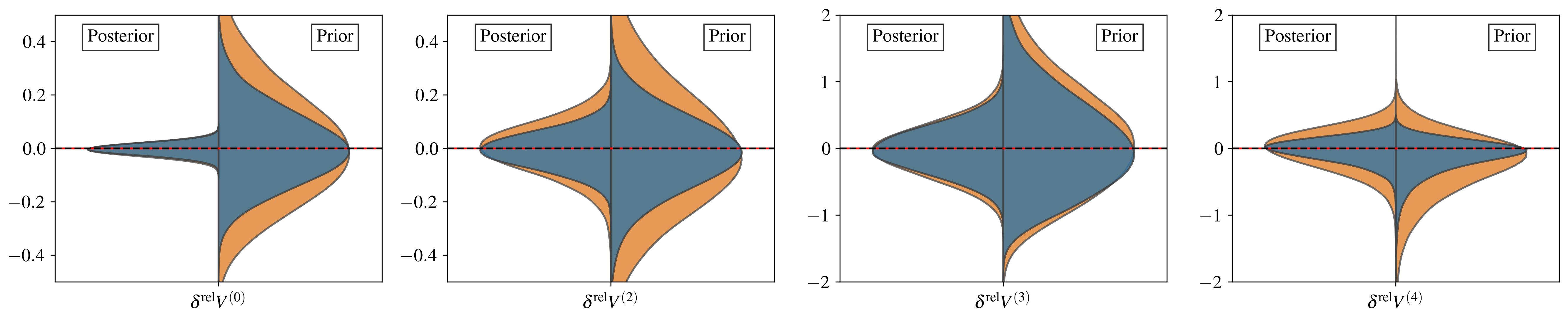
Figure 3: Same MCMC results as in Fig. 2, but here we sample the relative errors of various derivatives of the effective potential $\delta^{\mathrm{rel}}V^{(n)}$ with respect to the tortoise coordinate evaluated at the maximum. The right side of each violin plot shows the sampling from the prior distribution of all $\alpha^{(k)}$ simultaneously, with colors label the different $\alpha^{(k)}$ prior ranges: $\alpha^{(k)}_{\text{\tiny{P20}}}$ (blue) and $\alpha^{(k)}_{\text{\tiny{P10}}}$ (orange). The left side of each violin plot shows the sampling from the posterior distributions, with colors labeling the prior assumptions. We mark the injections (here corresponding to a Schwarzschild black hole) by red horizontal lines.

III Results

Using the techniques of the previous section, we now study two complementary settings. In the first setting (Sec. III.1) we perform injections assuming that GR is the correct theory of gravity. In the second setting (Sec. III.2) we assume a hypothetical modification with two non-zero deviation parameters – a nontrivial, but tractable case.

Within each setting we use the (complex) $l=2,$ $n=0,1$ QNM frequencies as hypothetical observations, with errors estimated by the Fisher matrix formalism as described in Sec. II.3. To explore the impact of different priors on the posteriors, we always use two different prior ranges ($\alpha^{(k)}_{\text{\tiny{P20}}}$ and $\alpha^{(k)}_{\text{\tiny{P10}}}$).

Within each of these two settings, we will address the inverse problem in two steps. We will first compare the posteriors for the parameters $\alpha^{(k)}$ in the optimistic scenario (where only one parameter varies) against the pessimistic scenario (where all parameters are varied simultaneously). Then, from the reconstruction of the potential, we will evaluate $V^{(p)}$ and compare it with the corresponding value $V^{(p)}_{\text{\tiny{GR}}}$ in GR by computing the relative difference

$$\delta^{\mathrm{rel}}V^{(p)}=\frac{V^{(p)}(r_{\mathrm{H}},\alpha^{(k)})-V^{(p)}_{\text{\tiny{GR}}}}{V^{(p)}_{\text{\tiny{GR}}}}.$$ (15)

III.1 Results for a GR injection

First we present our results under the assumption that GR is the correct theory of gravity.

The violin plots in Fig. 2 show the optimistic (left side) vs pessimistic (right side) posteriors for the Taylor expansion coefficients $\alpha^{(k)}$in Eq. (2). Different colors correspond to posteriors obtained with the two different (flat) prior ranges. In the optimistic case, it is possible to constrain all parameters independently of the chosen prior range. While the quantitative details of each optimistic bound are different and their widths increase with $k$ (as expected), they are qualitatively the same for all $k$. The situation is clearly different in the pessimistic case. Here the posterior distributions of all $\alpha^{(k)}$ have support at the prior boundaries, and they become broader when the prior range is increased. Since we allow for more parameters (12 in total: 11 $\alpha^{(k)}$’s and $r_{\mathrm{H}}$) than observed QNMs (4, i.e., 2 complex frequencies), this is not surprising.

In Fig. 3 we show the results for the WKB deviation coefficients $\delta^{\mathrm{rel}}V^{(n)}$ defined in Eq. (15). Since flat priors for $\alpha^{(k)}$ do not correspond to flat priors for $\delta^{\mathrm{rel}}V^{(n)}$, it is important to compare the posteriors with the priors. We want to understand if QNM frequencies contain information on the $\delta^{\mathrm{rel}}V^{(n)}$ coefficients, or if the inference is prior-dominated (in which case the QNMs would not be informative). We focus on the pessimistic posteriors, since the more general (pessimistic) assumption allows us to draw conservative conclusions. As usual, we show the two different prior ranges using different colors.

Quite remarkably, the posteriors for $\delta^{\mathrm{rel}}V^{(0)}$ are very robust, and they do not depend on the prior range choice. The posteriors for $\delta^{\mathrm{rel}}V^{(2)}$ and $\delta^{\mathrm{rel}}V^{(3)}$ are still more informative than the priors, but the QNM frequencies do not provide as much information as they do in the case of $\delta^{\mathrm{rel}}V^{(0)}$, and the measurement is even less informative in the case of $\delta^{\mathrm{rel}}V^{(4)}$. This is one of the main results of this paper: the “change of basis” from the $\alpha^{(k)}$’s to the $\delta^{\mathrm{rel}}V^{(n)}$’s (variables related to the light ring) is very effective, because QNMs carry physical information about the potential and its derivatives at the peak. This is in agreement with the conclusions of Ref. Völkel et al. (2022).

Note that the derivation of these results is fully independent of the WKB approximation: we never use the WKB approximation to compute the QNMs, but rather we use Leaver’s method to compute the injected QNM frequencies, and the parametrized framework of Eq. (4) to model their deviations from GR. The full MCMC analysis can capture correlations between the deviation parameters, as long as they are small enough to ensure the validity of the parametrized framework.

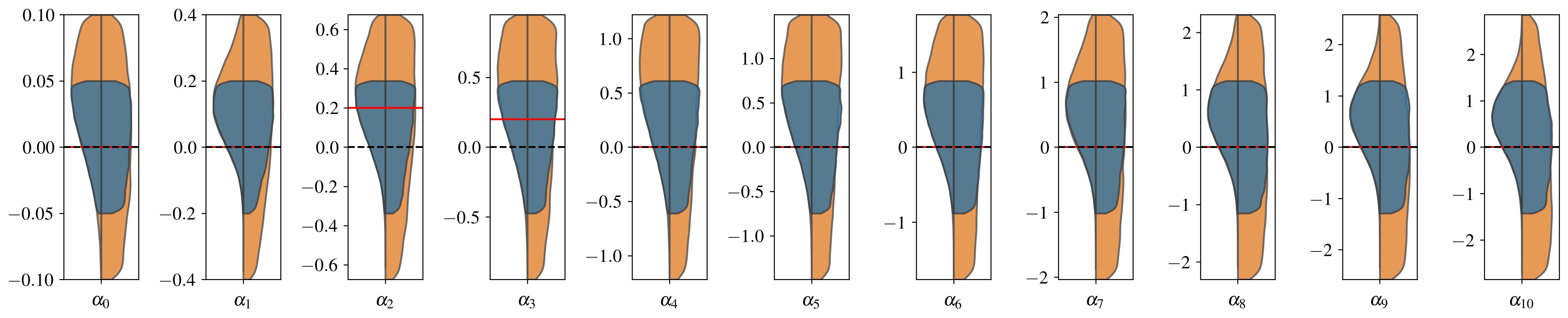
Figure 4: MCMC results for simulated observations of a modified Schwarzschild $n=0,1$ QNMs with relative errors described in the main text and assuming a prior for $r_{\mathrm{H}}$ corresponding to $5\,\%$ at $1\sigma$ confidence. The injected values (shown as horizontal red lines) are $\alpha^{(2)}=\alpha^{(3)}=0.2$, with all other values of $\alpha^{(k)}$ set equal to zero. From left to right we show the potential coefficients $\alpha^{(k)}$. In each panel, on the left side we plot the posteriors in the optimistic case (only one $\alpha^{(k)}$ is varied at a time), and on the right side we plot the posteriors in the pessimistic case (all $\alpha^{(k)}$’s are varied simultaneously). The blue (orange) color corresponds to a prior range of $\alpha^{(k)}_{\text{\tiny{P20}}}$ ($\alpha^{(k)}_{\text{\tiny{P10}}}$).

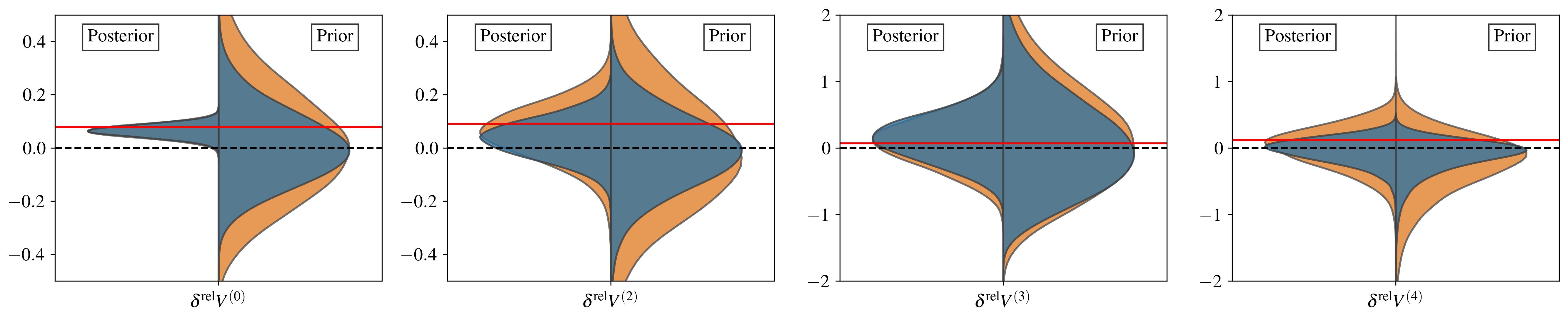
Figure 5: Same MCMC results as in Fig. 4, but here we sample the relative errors of various derivatives of the effective potential $\delta^{\mathrm{rel}}V^{(n)}$ with respect to the tortoise coordinate evaluated at the maximum. The right side of each violin plot shows the sampling from the prior distribution of all $\alpha^{(k)}$ simultaneously. The colors label the different $\alpha^{(k)}$ prior ranges, $\alpha^{(k)}_{\text{\tiny{P20}}}$ (blue) and $\alpha^{(k)}_{\text{\tiny{P10}}}$ (orange). The left side of each violin plot shows the sampling from the posterior distributions, with colors labeling the prior assumptions. We mark the injections by horizontal red lines.

III.2 Results for a non-GR injection

As an example of a possible non-GR injection, we consider the hypothetical case in which $\alpha^{(2)}=\alpha^{(3)}=0.2$, while all other $\alpha^{(k)}$’s are set to zero. We compute the QNM frequency with Leaver’s method, while we use the parametrized framework for the MCMC analysis.

In Fig. 4 we report the MCMC results, following the same notation and conventions as in Fig. 2. The injected values of $\alpha^{(k)}$ are marked by horizontal red lines. The plot shows that it is not possible to infer the correct values for any $\alpha^{(k)}$, except perhaps for $k=2$ and (less clearly) for $k=3$. The recovered values for all other $\alpha^{(k)}$’s peak away from their injected value. Some of the small-$k$ posteriors have strong support at the smaller prior limit, but they are well captured by the larger prior limit.

Given that these results are qualitatively very different from the GR injections, it is quite remarkable that the WKB-motivated constraints on the potential near the peak are as robust as before. In Fig. 5 we show that it is indeed possible to recover the non-GR injections (shown as red horizontal lines). The posterior of the dominant term $\delta^{\mathrm{rel}}V^{(0)}$ has tight support away from GR, while $\delta^{\mathrm{rel}}V^{(2)}$ is broader and has some overlap with the GR hypothesis. The higher derivatives for this injection are very close to their GR value, and the corresponding violin plots are almost indistinguishable from those of Fig. 3.

III.3 Theory-specific approach: a simple example

A theory-specific analysis can, in principle, be carried out in different ways. We could avoid making use of the parametrized framework and base it on a full MCMC analysis involving all free parameters of the theory. We could also, in principle, use the parametrized framework with the theory-predicted values of $\alpha^{(k)}$, which could depend on one (or multiple) coupling constants of the modified theory of gravity of interest. Instead of repeating a full MCMC analysis, here we show that the posteriors for $\delta^{\mathrm{rel}}V^{(0)}$ in the non-GR example above are already very informative when used in a “post-processing” analysis.

Let us assume, for simplicity, that the hypothetical modified theory predicts two non-zero deviation parameters, related to the only unknown parameter of the theory $\zeta$ as follows:

$$\alpha^{(2)}(\zeta)=\alpha^{(3)}(\zeta)=\zeta.$$ (16)

We use this trivial example just for illustrative purposes, but no fundamental limitation prevents us from relaxing these assumptions to allow for more than two non-zero deviation parameters, or to allow for a more complicated dependence of these parameters on $\zeta$. In fact, we would find qualitatively similar results if we assumed that $\alpha^{(3)}$ is suppressed by a small factor $\epsilon$.

By using Eq. (9) we can find the linear approximation for the modified potential $V^{(0)}(\zeta)$. The GR potential $V^{(0)}$ is known, so we can express the posteriors $\delta^{\mathrm{rel}}V^{(0)}$ in Fig. 5 (left side of the first violin plot) in terms of $V^{(0)}$. The posteriors are well approximated by a Gaussian, whose mean $\mu_{V}$ and width $\sigma_{V}$ we can fit numerically. Then we can insert the value of $\mu_{V}$ fitted to $V^{(0)}$ into Eq. (9), and invert it to find the most likely value of $\zeta$, which we will denote by $\mu_{\zeta}$. We can also estimate the $1\sigma$ and $2\sigma$ errors by repeating the inversion for $\mu_{V}\pm\sigma_{V}$ and $\mu_{V}\pm 2\sigma_{V}$. In Fig. 6 we show the results of this procedure. The injected value of the coupling parameter $\zeta$ is well within the $1\sigma$ constraint. The values of $\mu_{\zeta}$ and $\sigma_{\zeta}$ can also be used to define the theory-specific bounds on $\alpha^{(2)}(\zeta)$ and $\alpha^{(3)}(\zeta)$ in a similar way.

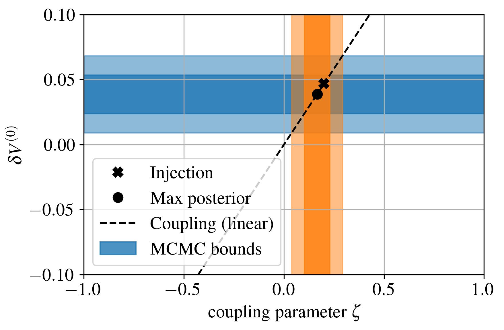
Figure 6: Post-processing analysis using the posterior of $V^{(0)}$. Blue areas show the $1\sigma$ and $2\sigma$ confidence levels of the theory-agnostic analysis, while the orange areas label the corresponding bounds on the theory-specific parameter $\zeta$. The black dashed line indicates the linear scaling predicted by Eq. (9). The black dot shows the maximum of the posterior, and the cross is the injected value.

If we do not know the precise form of $\alpha^{(2)}(\zeta),\alpha^{(3)}(\zeta)$ (i.e., in a theory-agnostic approach), we could treat them as independent variables in a post-processing analysis. From Eq. (9) we can find $\alpha^{(3)}$ as a function of $\alpha^{(2)}$ and $V^{(0)}$, with the results shown in Fig. 7. Once again, the injected value is within the $1\sigma$ confidence levels.

Finally, we could repeat the analysis by using the posteriors for $V^{(2)}$, which would in principle break the two-parameter degeneracy of the agnostic case. In practice, we find that the additional constraint is almost parallel to the constraint from $V^{(0)}$ and that it only excludes large values of the deviation parameters, for which the approximations do not hold anyway. These conclusions depend on the specific combination $\alpha^{(2)},\alpha^{(3)}$ that we have chosen in our example, and they may be qualitatively different for other combinations of the deviation parameters.

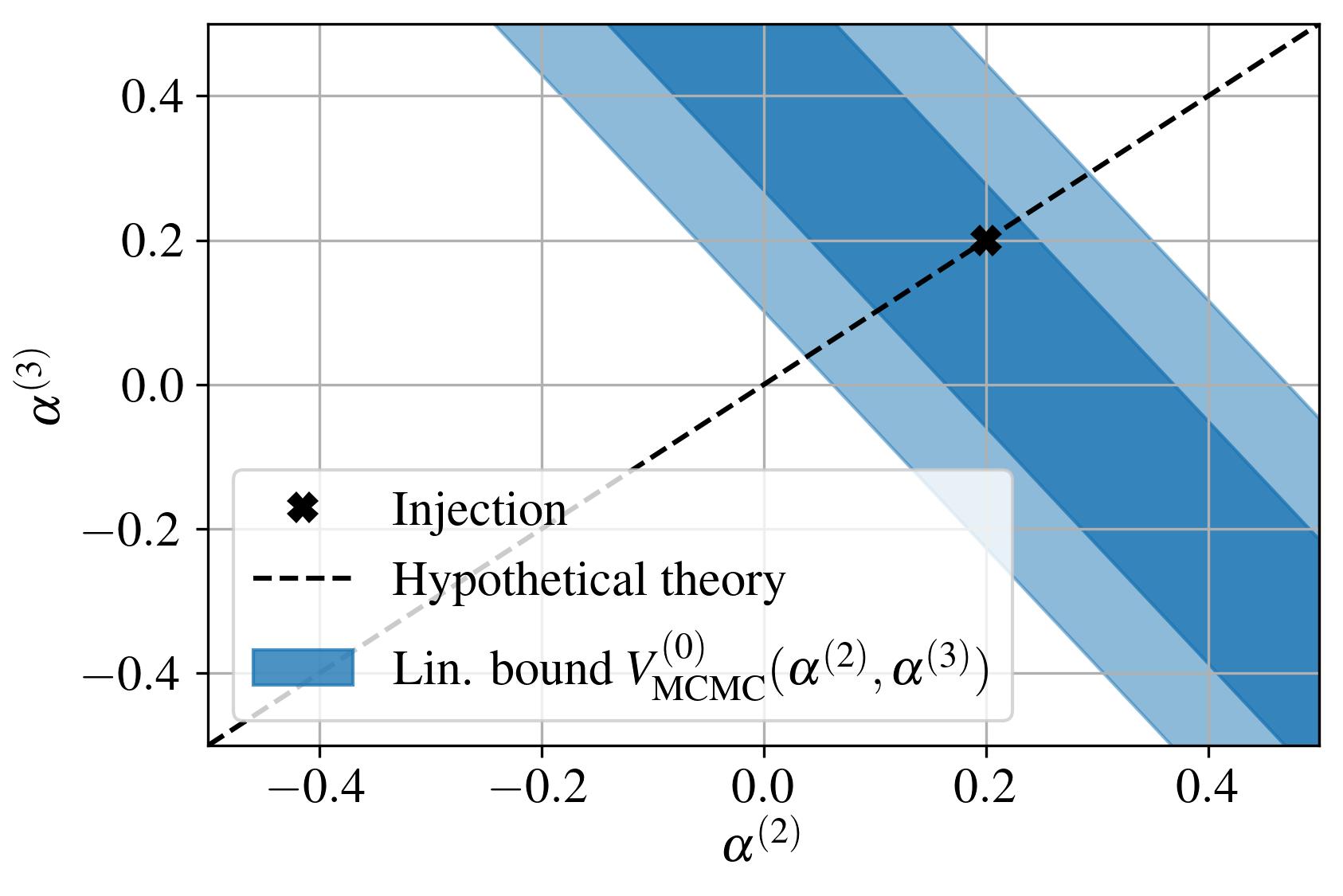
Figure 7: Post-processing analysis using the posterior of $V^{(0)}$. Blue areas show the $1\sigma$ and $2\sigma$ confidence levels on the functional relation $\alpha^{(3)}(\alpha^{(2)},V^{(0)})$. The black dashed line indicates the linear relation assumed in the hypothetical theory. The black dot is the intersection of the maximum of the posterior with the theory-specific relation, while the cross is the injected value.

IV Discussion and conclusions

In general, one may hope that modifications to the perturbation potential proportional to $\alpha^{(k)}\left(r_{\mathrm{H}}/r\right)^{k}$ would yield smaller corrections to the QNM spectrum as $k$ grows, as long as the coefficients $\alpha^{(k)}$ are comparable in order of magnitude. In fact, while this trend is present, the contributions from terms with $k\geq 2$ decay quite slowly. This lack of a strong hierarchy implies that, in general, it will be very difficult to recover the individual coefficients $\alpha^{(k)}$, at least in the absence of an underlying theory-specific ansatz. This was, indeed, the conclusion of previous work on parametrized ringdown using a principal component analysis Völkel et al. (2022).

Here we confirm this conclusion by exploring two specific cases: a GR QNM injection, and a non-GR injection. In both cases we look at two extreme scenarios: in the optimistic scenario we vary a single coefficient $\alpha^{(k)}$ at a time, and in the pessimistic scenario we let multiple $\alpha^{(k)}$’s (with $k=0,\dots 10$) vary simultaneously. In both scenarios we find that it is difficult to constrain the individual $\alpha^{(k)}$’s, as expected. We study a non-GR injection in which we assume that only two of the $\alpha^{(k)}$’s are non-zero. In the optimistic scenario we find that the posteriors of all of the $\alpha^{(k)}$’s disfavor GR, but only one of them is close to the correct injected value. Therefore it is difficult to identify which non-zero $\alpha^{(k)}$’s are present in the data without having more precise data, or additional (theory-specific) criteria to interpret the posteriors.

The main conclusion of this work is that the problem can be by-passed by exploiting the well-known relation between QNM frequencies and the properties of the perturbation potential at the light ring. This relation suggests that the complex correlations present when many $\alpha^{(k)}$’s are varied simultaneously can be understood by relating the $\alpha^{(k)}$’s to the value of the potential and its derivatives at the light ring. It is possible to obtain very robust constraints on the potential and its derivatives at the light ring, even in the pessimistic case in which many $\alpha^{(k)}$’s are varied simultaneously. More precisely, a measurement of the fundamental mode and of the first overtone can constrain quite precisely the value of the potential and of its second derivative evaluated at the peak. As demonstrated, this conclusion is not limited to GR injections, but it is also valid for non-GR injections.

We analyze, as a proof of principle, a hypothetical theory characterized by a single parameter $\zeta$, such that all non-zero deviations have the form $\alpha^{(k)}(\zeta)$. Through a simple “post-processing” analysis based on the inferred posterior for the value of the potential at the maximum, and assuming that only two of the $\alpha^{(k)}$’s are non-zero, we can recover the injected parameter $\zeta$ and estimate confidence intervals for each of the $\alpha^{(k)}$’s. This demonstrates that MCMC constraints on the value of the potential at the maximum can be used to find theory-specific properties, without rerunning a full MCMC analysis.

The intimate link between QNM frequencies and the potential at the light ring implies that there is a close relation between strong-gravity tests using black hole spectroscopy and the black hole shadow observations by the Event Horizon Telescope collaboration Akiyama et al. (2019a, b); Kocherlakota et al. (2021). In analogy with QNMs, the strong-field character of the shadow (which depends on the geometry near the light ring) also implies that the individual parameters in a PN expansion of the metric are hard to constrain, especially when many of them are allowed to vary simultaneously Völkel et al. (2021). Black hole shadow measurements can still constrain linear combinations of the metric and its derivative at the light ring Völkel et al. (2021), in a way which is closely reminiscent of the WKB results reported in this work.

In closing, it is important to discuss some caveats and possible future extensions of this work. The parametrized framework Cardoso et al. (2019); McManus et al. (2019) is only valid for non-rotating or slowly rotating black holes, but current gravitational-wave observations involve rotating black holes. More theory-dependent studies of QNMs for rotating black holes in modified theories of gravity are necessary to overcome this nontrivial obstacle, and to understand how a generalized parametrized framework can effectively be implemented and constrained. The increase in complexity resulting from the (generally nonseparable) perturbation equations in modified gravity implies that theory-specific tests may be particularly valuable, because they typically involve a small number of free parameters.

Appendix A Details for higher order WKB method

In this appendix we report some of the lengthy WKB expressions used in the main text. For convenience, we report again the WKB formula (6), up to third order:

$$\omega_{n}^{2}\simeq V^{(0)}-\mathrm{i}\sqrt{-2V^{(2)}}\alpha_{n}+\tilde{\Lambda}_{2}(n)+\tilde{\Lambda}_{3}(n)$$ (17)

Here $n$ is the QNM overtone number, $\alpha_{n}=n+1/2$, and the higher-order corrections read

$$\tilde{\Lambda}_{2}= \frac{1}{8}\left[\left(\frac{1}{4}+\alpha_{n}^{2}\right)\frac{V^{(4)}}{V^{(2)}}-\frac{1}{36}\left(7+60\alpha_{n}^{2}\right)\frac{{V^{(3)}}^{2}}{{V^{(2)}}^{2}}\right]\,,$$ (18)

$$\tilde{\Lambda}_{3}= -\frac{\mathrm{i}\alpha_{n}}{96\sqrt{-2V^{(2)}}}\Bigg{[}\frac{5}{72}\left(77+188\alpha_{n}^{2}\right)\frac{{V^{(3)}}^{4}}{{V^{(2)}}^{4}}$$

$$-\frac{1}{4}\left(51+100\alpha_{n}^{2}\right)\frac{{V^{(3)}}^{2}V^{(4)}}{{V^{(2)}}^{3}}$$

$$+\frac{1}{24}\left(67+68\alpha_{n}^{2}\right)\frac{{V^{(4)}}^{2}}{{V^{(2)}}^{2}}$$

$$+\frac{1}{3}\left(19+28\alpha_{n}^{2}\right)\frac{{V^{(3)}}V^{(5)}}{{V^{(2)}}^{2}}$$

$$-\frac{1}{3}\left(5+4\alpha_{n}^{2}\right)\frac{{V^{(6)}}}{{V^{(2)}}}\Bigg{]}\,.$$ (19)

References

- Abbott et al. (2016a) B. P. Abbott et al. (LIGO Scientific, Virgo), “Observation of Gravitational Waves from a Binary Black Hole Merger,” Phys. Rev. Lett. 116, 061102 (2016a), arXiv:1602.03837 [gr-qc] .
- Abbott et al. (2019a) B. P. Abbott et al. (LIGO Scientific, Virgo), “GWTC-1: A Gravitational-Wave Transient Catalog of Compact Binary Mergers Observed by LIGO and Virgo during the First and Second Observing Runs,” Phys. Rev. X 9, 031040 (2019a), arXiv:1811.12907 [astro-ph.HE] .
- Abbott et al. (2021a) R. Abbott et al. (LIGO Scientific, Virgo), “GWTC-2: Compact Binary Coalescences Observed by LIGO and Virgo During the First Half of the Third Observing Run,” Phys. Rev. X 11, 021053 (2021a), arXiv:2010.14527 [gr-qc] .
- Abbott et al. (2021b) R. Abbott et al. (LIGO Scientific, VIRGO, KAGRA), “GWTC-3: Compact Binary Coalescences Observed by LIGO and Virgo During the Second Part of the Third Observing Run,” (2021b), arXiv:2111.03606 [gr-qc] .
- Nitz et al. (2021) Alexander H. Nitz, Sumit Kumar, Yi-Fan Wang, Shilpa Kastha, Shichao Wu, Marlin Schäfer, Rahul Dhurkunde, and Collin D. Capano, “4-OGC: Catalog of gravitational waves from compact-binary mergers,” (2021), arXiv:2112.06878 [astro-ph.HE] .
- Olsen et al. (2022) Seth Olsen, Tejaswi Venumadhav, Jonathan Mushkin, Javier Roulet, Barak Zackay, and Matias Zaldarriaga (LIGO Scientific Collaboration, the Virgo), “New binary black hole mergers in the LIGO-Virgo O3a data,” Phys. Rev. D 106, 043009 (2022), arXiv:2201.02252 [astro-ph.HE] .
- Berti et al. (2015) Emanuele Berti et al., “Testing General Relativity with Present and Future Astrophysical Observations,” Class. Quant. Grav. 32, 243001 (2015), arXiv:1501.07274 [gr-qc] .
- Barack et al. (2019) Leor Barack et al., “Black holes, gravitational waves and fundamental physics: a roadmap,” Class. Quant. Grav. 36, 143001 (2019), arXiv:1806.05195 [gr-qc] .
- Yunes et al. (2016) Nicolas Yunes, Kent Yagi, and Frans Pretorius, “Theoretical Physics Implications of the Binary Black-Hole Mergers GW150914 and GW151226,” Phys. Rev. D 94, 084002 (2016), arXiv:1603.08955 [gr-qc] .
- Cardoso and Gualtieri (2016) Vitor Cardoso and Leonardo Gualtieri, “Testing the black hole ‘no-hair’ hypothesis,” Class. Quant. Grav. 33, 174001 (2016), arXiv:1607.03133 [gr-qc] .
- Berti et al. (2018a) Emanuele Berti, Kent Yagi, and Nicolás Yunes, “Extreme Gravity Tests with Gravitational Waves from Compact Binary Coalescences: (I) Inspiral-Merger,” Gen. Rel. Grav. 50, 46 (2018a), arXiv:1801.03208 [gr-qc] .
- Berti et al. (2018b) Emanuele Berti, Kent Yagi, Huan Yang, and Nicolás Yunes, “Extreme Gravity Tests with Gravitational Waves from Compact Binary Coalescences: (II) Ringdown,” Gen. Rel. Grav. 50, 49 (2018b), arXiv:1801.03587 [gr-qc] .
- Cardoso and Pani (2019) Vitor Cardoso and Paolo Pani, “Testing the nature of dark compact objects: a status report,” Living Rev. Rel. 22, 4 (2019), arXiv:1904.05363 [gr-qc] .
- Abbott et al. (2016b) B. P. Abbott et al. (LIGO Scientific, Virgo), “Tests of general relativity with GW150914,” Phys. Rev. Lett. 116, 221101 (2016b), [Erratum: Phys.Rev.Lett. 121, 129902 (2018)], arXiv:1602.03841 [gr-qc] .
- Abbott et al. (2019b) B. P. Abbott et al. (LIGO Scientific, Virgo), “Tests of General Relativity with the Binary Black Hole Signals from the LIGO-Virgo Catalog GWTC-1,” Phys. Rev. D 100, 104036 (2019b), arXiv:1903.04467 [gr-qc] .
- Abbott et al. (2021c) R. Abbott et al. (LIGO Scientific, Virgo), “Tests of general relativity with binary black holes from the second LIGO-Virgo gravitational-wave transient catalog,” Phys. Rev. D 103, 122002 (2021c), arXiv:2010.14529 [gr-qc] .
- Abbott et al. (2021d) R. Abbott et al. (LIGO Scientific, VIRGO, KAGRA), “Tests of General Relativity with GWTC-3,” (2021d), arXiv:2112.06861 [gr-qc] .
- Ghosh et al. (2021) Abhirup Ghosh, Richard Brito, and Alessandra Buonanno, “Constraints on quasinormal-mode frequencies with LIGO-Virgo binary–black-hole observations,” Phys. Rev. D 103, 124041 (2021), arXiv:2104.01906 [gr-qc] .
- Detweiler (1980) Steven L. Detweiler, “Black holes and gravitational waves. III. The resonant frequencies of rotating holes,” Astrophys. J. 239, 292–295 (1980).
- Dreyer et al. (2004) Olaf Dreyer, Bernard J. Kelly, Badri Krishnan, Lee Samuel Finn, David Garrison, and Ramon Lopez-Aleman, “Black hole spectroscopy: Testing general relativity through gravitational wave observations,” Class. Quant. Grav. 21, 787–804 (2004), arXiv:gr-qc/0309007 .
- Berti et al. (2006) Emanuele Berti, Vitor Cardoso, and Clifford M. Will, “On gravitational-wave spectroscopy of massive black holes with the space interferometer LISA,” Phys. Rev. D 73, 064030 (2006), arXiv:gr-qc/0512160 .
- Isi et al. (2019) Maximiliano Isi, Matthew Giesler, Will M. Farr, Mark A. Scheel, and Saul A. Teukolsky, “Testing the no-hair theorem with GW150914,” Phys. Rev. Lett. 123, 111102 (2019), arXiv:1905.00869 [gr-qc] .
- Capano et al. (2021) Collin D. Capano, Miriam Cabero, Julian Westerweck, Jahed Abedi, Shilpa Kastha, Alexander H. Nitz, Alex B. Nielsen, and Badri Krishnan, “Observation of a multimode quasi-normal spectrum from a perturbed black hole,” (2021), arXiv:2105.05238 [gr-qc] .
- Cotesta et al. (2022) Roberto Cotesta, Gregorio Carullo, Emanuele Berti, and Vitor Cardoso, “Analysis of Ringdown Overtones in GW150914,” Phys. Rev. Lett. 129, 111102 (2022), arXiv:2201.00822 [gr-qc] .
- Finch and Moore (2022) Eliot Finch and Christopher J. Moore, “Searching for a ringdown overtone in GW150914,” Phys. Rev. D 106, 043005 (2022), arXiv:2205.07809 [gr-qc] .
- Isi and Farr (2022) Maximiliano Isi and Will M. Farr, “Revisiting the ringdown of GW150914,” (2022), arXiv:2202.02941 [gr-qc] .
- Capano et al. (2022) Collin D. Capano, Jahed Abedi, Shilpa Kastha, Alexander H. Nitz, Julian Westerweck, Yi-Fan Wang, Miriam Cabero, Alex B. Nielsen, and Badri Krishnan, “Statistical validation of the detection of a sub-dominant quasi-normal mode in GW190521,” (2022), arXiv:2209.00640 [gr-qc] .
- Sberna et al. (2022) Laura Sberna, Pablo Bosch, William E. East, Stephen R. Green, and Luis Lehner, “Nonlinear effects in the black hole ringdown: Absorption-induced mode excitation,” Phys. Rev. D 105, 064046 (2022), arXiv:2112.11168 [gr-qc] .
- Cheung et al. (2022) Mark Ho-Yeuk Cheung et al., “Nonlinear effects in black hole ringdown,” (2022), arXiv:2208.07374 [gr-qc] .
- Mitman et al. (2022) Keefe Mitman et al., “Nonlinearities in black hole ringdowns,” (2022), arXiv:2208.07380 [gr-qc] .
- Berti et al. (2007) Emanuele Berti, Jaime Cardoso, Vitor Cardoso, and Marco Cavaglia, “Matched-filtering and parameter estimation of ringdown waveforms,” Phys. Rev. D 76, 104044 (2007), arXiv:0707.1202 [gr-qc] .
- Baibhav et al. (2018) Vishal Baibhav, Emanuele Berti, Vitor Cardoso, and Gaurav Khanna, “Black Hole Spectroscopy: Systematic Errors and Ringdown Energy Estimates,” Phys. Rev. D 97, 044048 (2018), arXiv:1710.02156 [gr-qc] .
- Giesler et al. (2019) Matthew Giesler, Maximiliano Isi, Mark A. Scheel, and Saul Teukolsky, “Black Hole Ringdown: The Importance of Overtones,” Phys. Rev. X 9, 041060 (2019), arXiv:1903.08284 [gr-qc] .
- Ota and Chirenti (2020) Iara Ota and Cecilia Chirenti, “Overtones or higher harmonics? Prospects for testing the no-hair theorem with gravitational wave detections,” Phys. Rev. D 101, 104005 (2020), arXiv:1911.00440 [gr-qc] .
- Bhagwat et al. (2020a) Swetha Bhagwat, Xisco Jimenez Forteza, Paolo Pani, and Valeria Ferrari, “Ringdown overtones, black hole spectroscopy, and no-hair theorem tests,” Phys. Rev. D 101, 044033 (2020a), arXiv:1910.08708 [gr-qc] .
- Bhagwat et al. (2020b) Swetha Bhagwat, Miriam Cabero, Collin D. Capano, Badri Krishnan, and Duncan A. Brown, “Detectability of the subdominant mode in a binary black hole ringdown,” Phys. Rev. D 102, 024023 (2020b), arXiv:1910.13203 [gr-qc] .
- Cook (2020) Gregory B. Cook, “Aspects of multimode Kerr ringdown fitting,” Phys. Rev. D 102, 024027 (2020), arXiv:2004.08347 [gr-qc] .
- Bustillo et al. (2021) Juan Calderón Bustillo, Paul D. Lasky, and Eric Thrane, “Black-hole spectroscopy, the no-hair theorem, and GW150914: Kerr versus Occam,” Phys. Rev. D 103, 024041 (2021), arXiv:2010.01857 [gr-qc] .
- Jiménez Forteza et al. (2020) Xisco Jiménez Forteza, Swetha Bhagwat, Paolo Pani, and Valeria Ferrari, “Spectroscopy of binary black hole ringdown using overtones and angular modes,” Phys. Rev. D 102, 044053 (2020), arXiv:2005.03260 [gr-qc] .
- Magaña Zertuche et al. (2022) Lorena Magaña Zertuche et al., “High Precision Ringdown Modeling: Multimode Fits and BMS Frames,” Phys. Rev. D 105, 104015 (2022), arXiv:2110.15922 [gr-qc] .
- Berti et al. (2016) Emanuele Berti, Alberto Sesana, Enrico Barausse, Vitor Cardoso, and Krzysztof Belczynski, “Spectroscopy of Kerr black holes with Earth- and space-based interferometers,” Phys. Rev. Lett. 117, 101102 (2016), arXiv:1605.09286 [gr-qc] .
- Cabero et al. (2020) Miriam Cabero, Julian Westerweck, Collin D. Capano, Sumit Kumar, Alex B. Nielsen, and Badri Krishnan, “Black hole spectroscopy in the next decade,” Phys. Rev. D 101, 064044 (2020), arXiv:1911.01361 [gr-qc] .
- Ota and Chirenti (2022) Iara Ota and Cecilia Chirenti, “Black hole spectroscopy horizons for current and future gravitational wave detectors,” Phys. Rev. D 105, 044015 (2022), arXiv:2108.01774 [gr-qc] .
- Bhagwat et al. (2022) Swetha Bhagwat, Costantino Pacilio, Enrico Barausse, and Paolo Pani, “Landscape of massive black-hole spectroscopy with LISA and the Einstein Telescope,” Phys. Rev. D 105, 124063 (2022), arXiv:2201.00023 [gr-qc] .
- Tattersall et al. (2018) Oliver J. Tattersall, Pedro G. Ferreira, and Macarena Lagos, “General theories of linear gravitational perturbations to a Schwarzschild Black Hole,” Phys. Rev. D 97, 044021 (2018), arXiv:1711.01992 [gr-qc] .
- Cardoso et al. (2019) Vitor Cardoso, Masashi Kimura, Andrea Maselli, Emanuele Berti, Caio F. B. Macedo, and Ryan McManus, “Parametrized black hole quasinormal ringdown: Decoupled equations for nonrotating black holes,” Phys. Rev. D 99, 104077 (2019), arXiv:1901.01265 [gr-qc] .
- McManus et al. (2019) Ryan McManus, Emanuele Berti, Caio F. B. Macedo, Masashi Kimura, Andrea Maselli, and Vitor Cardoso, “Parametrized black hole quasinormal ringdown. II. Coupled equations and quadratic corrections for nonrotating black holes,” Phys. Rev. D 100, 044061 (2019), arXiv:1906.05155 [gr-qc] .
- Völkel et al. (2022) Sebastian H. Völkel, Nicola Franchini, and Enrico Barausse, “Theory-agnostic reconstruction of potential and couplings from quasinormal modes,” Phys. Rev. D 105, 084046 (2022), arXiv:2202.08655 [gr-qc] .
- Völkel and Barausse (2020) Sebastian H. Völkel and Enrico Barausse, “Bayesian Metric Reconstruction with Gravitational Wave Observations,” Phys. Rev. D 102, 084025 (2020), arXiv:2007.02986 [gr-qc] .
- Konoplya and Zhidenko (2022) R. A. Konoplya and A. Zhidenko, “First few overtones probe the event horizon geometry,” (2022), arXiv:2209.00679 [gr-qc] .
- Meidam et al. (2014) J. Meidam, M. Agathos, C. Van Den Broeck, J. Veitch, and B. S. Sathyaprakash, “Testing the no-hair theorem with black hole ringdowns using TIGER,” Phys. Rev. D 90, 064009 (2014), arXiv:1406.3201 [gr-qc] .
- Maselli et al. (2020) Andrea Maselli, Paolo Pani, Leonardo Gualtieri, and Emanuele Berti, “Parametrized ringdown spin expansion coefficients: a data-analysis framework for black-hole spectroscopy with multiple events,” Phys. Rev. D 101, 024043 (2020), arXiv:1910.12893 [gr-qc] .
- Carullo (2021) Gregorio Carullo, “Enhancing modified gravity detection from gravitational-wave observations using the parametrized ringdown spin expansion coeffcients formalism,” Phys. Rev. D 103, 124043 (2021), arXiv:2102.05939 [gr-qc] .
- Yang et al. (2017) Huan Yang, Kent Yagi, Jonathan Blackman, Luis Lehner, Vasileios Paschalidis, Frans Pretorius, and Nicolás Yunes, “Black hole spectroscopy with coherent mode stacking,” Phys. Rev. Lett. 118, 161101 (2017), arXiv:1701.05808 [gr-qc] .
- Press (1971) William H. Press, “Long Wave Trains of Gravitational Waves from a Vibrating Black Hole,” Astrophys. J. Lett. 170, L105–L108 (1971).
- Schutz and Will (1985) Bernard F. Schutz and Clifford M. Will, “Black Hole Normal Modes: a Semianalytical Approach,” Astrophys. J. Lett. 291, L33–L36 (1985).
- Cardoso et al. (2009) Vitor Cardoso, Alex S. Miranda, Emanuele Berti, Helvi Witek, and Vilson T. Zanchin, “Geodesic stability, Lyapunov exponents and quasinormal modes,” Phys. Rev. D 79, 064016 (2009), arXiv:0812.1806 [hep-th] .
- Iyer and Will (1987) Sai Iyer and Clifford M. Will, “Black Hole Normal Modes: A WKB Approach. 1. Foundations and Application of a Higher Order WKB Analysis of Potential Barrier Scattering,” Phys. Rev. D 35, 3621 (1987).
- Konoplya (2003) R. A. Konoplya, “Quasinormal behavior of the d-dimensional Schwarzschild black hole and higher order WKB approach,” Phys. Rev. D 68, 024018 (2003), arXiv:gr-qc/0303052 .
- Matyjasek and Opala (2017) Jerzy Matyjasek and Michał Opala, “Quasinormal modes of black holes. The improved semianalytic approach,” Phys. Rev. D 96, 024011 (2017), arXiv:1704.00361 [gr-qc] .
- Glampedakis et al. (2017) Kostas Glampedakis, George Pappas, Hector O. Silva, and Emanuele Berti, “Post-Kerr black hole spectroscopy,” Phys. Rev. D 96, 064054 (2017), arXiv:1706.07658 [gr-qc] .
- Glampedakis and Silva (2019) Kostas Glampedakis and Hector O. Silva, “Eikonal quasinormal modes of black holes beyond General Relativity,” Phys. Rev. D 100, 044040 (2019), arXiv:1906.05455 [gr-qc] .
- Silva and Glampedakis (2020) Hector O. Silva and Kostas Glampedakis, “Eikonal quasinormal modes of black holes beyond general relativity. II. Generalized scalar-tensor perturbations,” Phys. Rev. D 101, 044051 (2020), arXiv:1912.09286 [gr-qc] .
- Bryant et al. (2021) Albert Bryant, Hector O. Silva, Kent Yagi, and Kostas Glampedakis, “Eikonal quasinormal modes of black holes beyond general relativity. III. Scalar Gauss-Bonnet gravity,” Phys. Rev. D 104, 044051 (2021), arXiv:2106.09657 [gr-qc] .
- Akiyama et al. (2019a) Kazunori Akiyama et al. (Event Horizon Telescope), “First M87 Event Horizon Telescope Results. I. The Shadow of the Supermassive Black Hole,” Astrophys. J. Lett. 875, L1 (2019a), arXiv:1906.11238 [astro-ph.GA] .
- Akiyama et al. (2019b) Kazunori Akiyama et al. (Event Horizon Telescope), “First M87 Event Horizon Telescope Results. VI. The Shadow and Mass of the Central Black Hole,” Astrophys. J. Lett. 875, L6 (2019b), arXiv:1906.11243 [astro-ph.GA] .
- Völkel et al. (2021) Sebastian H. Völkel, Enrico Barausse, Nicola Franchini, and Avery E. Broderick, “EHT tests of the strong-field regime of general relativity,” Class. Quant. Grav. 38, 21LT01 (2021), arXiv:2011.06812 [gr-qc] .
- Kocherlakota et al. (2021) Prashant Kocherlakota et al. (Event Horizon Telescope), “Constraints on black-hole charges with the 2017 EHT observations of M87*,” Phys. Rev. D 103, 104047 (2021), arXiv:2105.09343 [gr-qc] .
- Regge and Wheeler (1957) Tullio Regge and John A. Wheeler, “Stability of a Schwarzschild singularity,” Phys. Rev. 108, 1063–1069 (1957).
- Zerilli (1970) Frank J. Zerilli, “Effective potential for even parity Regge-Wheeler gravitational perturbation equations,” Phys. Rev. Lett. 24, 737–738 (1970).
- Teukolsky (1973) Saul A. Teukolsky, “Perturbations of a rotating black hole. 1. Fundamental equations for gravitational electromagnetic and neutrino field perturbations,” Astrophys. J. 185, 635–647 (1973).
- Kokkotas and Schmidt (1999) Kostas D. Kokkotas and Bernd G. Schmidt, “Quasinormal modes of stars and black holes,” Living Rev. Rel. 2, 2 (1999), arXiv:gr-qc/9909058 .
- Nollert (1999) Hans-Peter Nollert, “TOPICAL REVIEW: Quasinormal modes: the characteristic ‘sound’ of black holes and neutron stars,” Class. Quant. Grav. 16, R159–R216 (1999).
- Berti et al. (2009) Emanuele Berti, Vitor Cardoso, and Andrei O. Starinets, “Quasinormal modes of black holes and black branes,” Class. Quant. Grav. 26, 163001 (2009), arXiv:0905.2975 [gr-qc] .
- Konoplya and Zhidenko (2011) R. A. Konoplya and A. Zhidenko, “Quasinormal modes of black holes: From astrophysics to string theory,” Rev. Mod. Phys. 83, 793–836 (2011), arXiv:1102.4014 [gr-qc] .
- Pani (2013) Paolo Pani, “Advanced Methods in Black-Hole Perturbation Theory,” Int. J. Mod. Phys. A 28, 1340018 (2013), arXiv:1305.6759 [gr-qc] .
- Cardoso and Gualtieri (2009) Vitor Cardoso and Leonardo Gualtieri, “Perturbations of Schwarzschild black holes in Dynamical Chern-Simons modified gravity,” Phys. Rev. D 80, 064008 (2009), [Erratum: Phys.Rev.D 81, 089903 (2010)], arXiv:0907.5008 [gr-qc] .
- Molina et al. (2010) C. Molina, Paolo Pani, Vitor Cardoso, and Leonardo Gualtieri, “Gravitational signature of Schwarzschild black holes in dynamical Chern-Simons gravity,” Phys. Rev. D 81, 124021 (2010), arXiv:1004.4007 [gr-qc] .
- Blázquez-Salcedo et al. (2016) Jose Luis Blázquez-Salcedo, Caio F. B. Macedo, Vitor Cardoso, Valeria Ferrari, Leonardo Gualtieri, Fech Scen Khoo, Jutta Kunz, and Paolo Pani, “Perturbed black holes in Einstein-dilaton-Gauss-Bonnet gravity: Stability, ringdown, and gravitational-wave emission,” Phys. Rev. D 94, 104024 (2016), arXiv:1609.01286 [gr-qc] .
- Blázquez-Salcedo et al. (2017) Jose Luis Blázquez-Salcedo, Fech Scen Khoo, and Jutta Kunz, “Quasinormal modes of Einstein-Gauss-Bonnet-dilaton black holes,” Phys. Rev. D 96, 064008 (2017), arXiv:1706.03262 [gr-qc] .
- Blázquez-Salcedo et al. (2020a) Jose Luis Blázquez-Salcedo, Daniela D. Doneva, Sarah Kahlen, Jutta Kunz, Petya Nedkova, and Stoytcho S. Yazadjiev, “Axial perturbations of the scalarized Einstein-Gauss-Bonnet black holes,” Phys. Rev. D 101, 104006 (2020a), arXiv:2003.02862 [gr-qc] .
- Blázquez-Salcedo et al. (2020b) Jose Luis Blázquez-Salcedo, Daniela D. Doneva, Sarah Kahlen, Jutta Kunz, Petya Nedkova, and Stoytcho S. Yazadjiev, “Polar quasinormal modes of the scalarized Einstein-Gauss-Bonnet black holes,” Phys. Rev. D 102, 024086 (2020b), arXiv:2006.06006 [gr-qc] .
- Franchini et al. (2021) Nicola Franchini, Mario Herrero-Valea, and Enrico Barausse, “Relation between general relativity and a class of Hořava gravity theories,” Phys. Rev. D 103, 084012 (2021), arXiv:2103.00929 [gr-qc] .
- Wagle et al. (2022) Pratik Wagle, Nicolas Yunes, and Hector O. Silva, “Quasinormal modes of slowly-rotating black holes in dynamical Chern-Simons gravity,” Phys. Rev. D 105, 124003 (2022), arXiv:2103.09913 [gr-qc] .
- Srivastava et al. (2021) Manu Srivastava, Yanbei Chen, and S. Shankaranarayanan, “Analytical computation of quasinormal modes of slowly rotating black holes in dynamical Chern-Simons gravity,” Phys. Rev. D 104, 064034 (2021), arXiv:2106.06209 [gr-qc] .
- Pierini and Gualtieri (2021) Lorenzo Pierini and Leonardo Gualtieri, “Quasi-normal modes of rotating black holes in Einstein-dilaton Gauss-Bonnet gravity: the first order in rotation,” Phys. Rev. D 103, 124017 (2021), arXiv:2103.09870 [gr-qc] .
- Pierini and Gualtieri (2022) Lorenzo Pierini and Leonardo Gualtieri, “Quasi-normal modes of rotating black holes in Einstein-dilaton Gauss-Bonnet gravity: the second order in rotation,” (2022), arXiv:2207.11267 [gr-qc] .
- Cano et al. (2020) Pablo A. Cano, Kwinten Fransen, and Thomas Hertog, “Ringing of rotating black holes in higher-derivative gravity,” Phys. Rev. D 102, 044047 (2020), arXiv:2005.03671 [gr-qc] .
- Cano et al. (2022) Pablo A. Cano, Kwinten Fransen, Thomas Hertog, and Simon Maenaut, “Gravitational ringing of rotating black holes in higher-derivative gravity,” Phys. Rev. D 105, 024064 (2022), arXiv:2110.11378 [gr-qc] .
- Li et al. (2022) Dongjun Li, Pratik Wagle, Yanbei Chen, and Nicolás Yunes, “Perturbations of spinning black holes beyond General Relativity: Modified Teukolsky equation,” (2022), arXiv:2206.10652 [gr-qc] .
- Hussain and Zimmerman (2022) Asad Hussain and Aaron Zimmerman, “An approach to computing spectral shifts for black holes beyond Kerr,” (2022), arXiv:2206.10653 [gr-qc] .
- Kimura (2020) Masashi Kimura, “Note on the parametrized black hole quasinormal ringdown formalism,” Phys. Rev. D 101, 064031 (2020), arXiv:2001.09613 [gr-qc] .
- Konoplya et al. (2019) R. A. Konoplya, A. Zhidenko, and A. F. Zinhailo, “Higher order WKB formula for quasinormal modes and grey-body factors: recipes for quick and accurate calculations,” Class. Quant. Grav. 36, 155002 (2019), arXiv:1904.10333 [gr-qc] .
- Foreman-Mackey et al. (2013) Daniel Foreman-Mackey, David W. Hogg, Dustin Lang, and Jonathan Goodman, “emcee: The MCMC Hammer,” Publ. Astron. Soc. Pac. 125, 306–312 (2013), arXiv:1202.3665 [astro-ph.IM] .
- Goodman and Weare (2010) Jonathan Goodman and Jonathan Weare, “Ensemble samplers with affine invariance,” Communications in Applied Mathematics and Computational Science 5, 65–80 (2010).
- Stanzione et al. (2020) Dan Stanzione, John West, R. Todd Evans, Tommy Minyard, Omar Ghattas, and Dhabaleswar K. Panda, “Frontera: The evolution of leadership computing at the national science foundation,” in Practice and Experience in Advanced Research Computing, PEARC ’20 (Association for Computing Machinery, New York, NY, USA, 2020) p. 106–111.