SGC: A semi-supervised pipeline for gene clustering using self-training approach in gene co-expression networks
Abstract
A widely used approach for extracting information from gene expression data employ the construction of a gene co-expression network and the subsequent application of algorithms that discover network structure. In particular, a common goal is the computational discovery of gene clusters, commonly called modules. When applied on a novel gene expression dataset, the quality of the computed modules can be evaluated automatically, using Gene Ontology enrichment, a method that measures the frequencies of Gene Ontology terms in the computed modules and evaluates their statistical likelihood. In this work we propose SGC a novel pipeline for gene clustering based on relatively recent seminal work in the mathematics of spectral network theory. SGC consists of multiple novel steps that enable the computation of highly enriched modules in an unsupervised manner. But unlike all existing frameworks, it further incorporates a novel step that leverages Gene Ontology information in a semi-supervised clustering method that further improves the quality of the computed modules. Comparing with already well-known existing frameworks, we show that SGC results in higher enrichment in real data. In particular, in real gene expression datasets, SGC outperforms in all except one.
1 Introduction
High throughput gene expression data enables gene functionality understanding in fully systematic frameworks. Gene module detection in Gene Co-expression Networks (GCNs) is a prominent such framework that has generated multiple insights, from unraveling the biological process of plant organisms [Emamjomeh2017] and essential genes in microalgae [Panahi2021], to assigning unknown genes to biological functions [Ma2018] and recognizing disease mechanisms [Parsana2019], e.g. for coronary artery disease [Liu2016].
GCNs are graph-based models where nodes correspond to genes and the strength of the link between each pair of nodes is a measure of similarity in the expression behavior of the two genes [Tieri2019]. The goal is to group the genes in a way that those with similar expression pattern fall within the same network cluster, commonly called module [Gat2003, Sipko2017]. GCNs are constructed by applying a similarity measure on the expression measurements of gene pairs. Genes are then clustered using unsupervised graph clustering algorithms. Finally the modules are analyzed and interpreted for gene functionality [niloo2021].
The de facto standard automatic technique for module quality analysis is Gene Ontology (GO) enrichment, a method that reveals if a module of co-expressed genes is enriched for genes that belong to known pathways or functions. Enrichment is a measure of module quality and the module-enriching GO terms can be used to discover biological meaning [Khatri2005, niloo2021, Botia2017, Russo2018]. Statistically, in a given module, this method determines the significance of the GO terms for a test query by associating p-values . The query includes the test direction, either “underrepresented” (under) or “overrepresented” (over), and three ontologies; “biological process” (BP), “cellular component” (CC), and “molecular function” (MF). p-values are derived based on the number of observed genes in a specific query with the number of genes that might appear in the same query if a selection performed from the same pool were completely random. In effect, this values identify if the GO terms that appear more frequently than would be expected by chance [Khatri2005]. As usual the smaller the p-value the more significant the GO term.
1.1 Background on existing GCN frameworks
Several frameworks and algorithms have been developed for GCNs construction and analysis such as [Zhang2005general, Lan2008, petal2015, coseq, CoXpress, Botia2017, Russo2018]. Among them Weighted Correlation Network Analysis (WGCNA) [Lan2008], is still the most widely accepted and used framework for module detection in GCNs [niloo2021, Botia2017, Russo2018, Liu2016, Hou2021]. WGCNA uses the Pearson correlation of gene expressions to form a ‘provisional’ network and then powers the strength values on its links so that the network conforms with a “scale-freeness” criterion. The final network is constructed by adding to the provisional network additional second-order neighborhood information, in the form of what is called topological overlap measure (TOM). Finally, WGCNA uses a standard hierarchical clustering (HC) algorithm to produce modules [dynamicTreeCut].
In recent years, there has been a growing interest to enhance WGCNA and multiple frameworks have been proposed as a modification of this framework. These pipelines mainly utilize an additional step in the form of either pre-processing or post-processing to WGCNA. Co-Expression Modules identification Tool (CEMiTool) is a pipeline that incorporates an extra pre-processing step to filter the genes using the inverse gamma distribution [Russo2018]. In another study, it is shown that a calibration pre-processing step in raw gene expression data results in increased GO enrichment [niloo2021]. Two other frameworks, the popular CoExpNets [Botia2017] and K-Module [Hou2021], have utilized k-means clustering [KMeans] as a post-processing step to the output of WGCNA. Finally, in a comparative study, it is revealed that CEMiTool has advantage over WGCNA [Cheng2020].
1.2 Our framework: Self-trained Gene Clustering
We have developed Self-training Gene Clustering (SGC), a user-friendly R package for GCNs construction and analysis. Its integration with Bioconductor makes it easy to use and apply. SGC differentiates itself from WGCNA and other pipelines in three key ways: (i) It constructs a network without relying on the scale-freeness criterion which has been controversial [SChaefer2017, Raya2006, Lima2009, Broido2019, Clote2020]. (ii) It clusters the network using a variant of spectral graph clustering that has been proposed relatively recently in seminal work [Cheeger]. (iii) It incorporates ‘self-training’, a supervised clustering step that GO enrichment information obtained from the previous step and further enhances the quality of the modules. To our knowledge SGC is the first pipeline that uses GO enrichment information as supervision.
1.2.1 SGC: The workflow
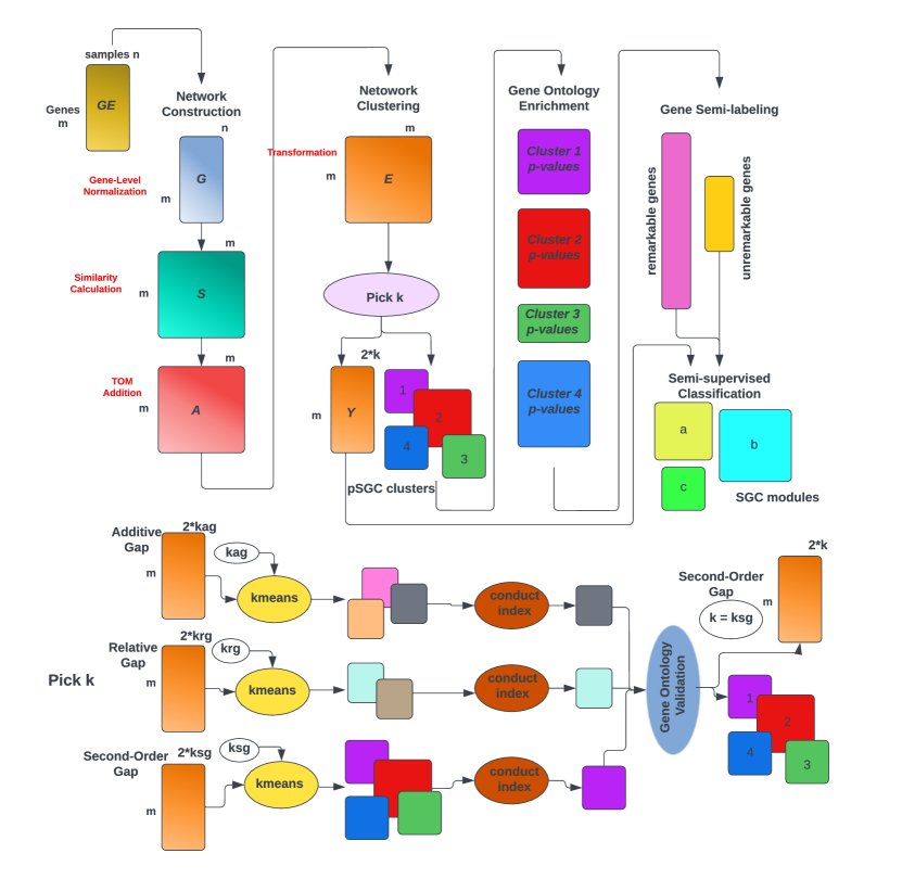
The workflow of SGC is illustrated in figure Figure 1; in what follows we give an overview of SGC and also point to the corresponding sections containing more details. SGC takes as input a gene expression matrix with genes and sample and performs the following five main steps:
Network Construction: Each gene vector, i.e. each row in matrix is normalized to a unit vector; this results to a matrix . Next, the Gaussian kernel function is used as the similarity metric to calculate in which and shows the similarity value between gene and . Then, the second-order neighborhood information will be added to the network in the form of topological overlap measure (TOM) [Zhang2005general]. The result of this step is an symmetric adjacency matrix . [Section 2.1.1]
Network Clustering: Matrix is used to define and solve an appropriate eigenvalue problem. The eigenvalues are used to determine three potential values for the number of clusters ([Section 2.1.2]). For each such value of , SGC computes a clustering of the network, by applying the kmeans algorithm on an embedding matrix generated from eigenvectors. In each clustering it finds a test cluster, defined as the cluster with the smallest conductance index. The three test clusters are evaluated for GO enrichment, and SGC picks the clustering that yielded the test cluster with highest GO enrichment. This clustering is the output of the Network Clustering step, and its clusters are the initial clusters. [Section 2.1.2]
Gene Ontology Enrichment: GO enrichment analysis is carried out on the initial clusters individually. [Section 2.1.3]
Gene semi-labeling: Genes are categorized into remarkable genes and unremarkable genes using information derived from the GO enrichment step. For each cluster, remarkable genes are those that have contributed to GO terms that are more significant relative to a baseline. Remarkable genes are labeled according to their corresponding cluster label. Not all clusters contain remarkable genes, and thus a new number of clusters is determined, and accordingly, labels are assigned to the remarkable genes and to the corresponding geometric points in the embedding matrix computed in the Network Clustering step. This defines a supervised classification problem.
Semi-supervised classification: The supervised classification problem is solved with an appropriately selected and configured machine learning algorithm (either k-nearest neighbors [bishop], or one-vs-rest logistic regression [bishop]) with the remarkable genes as the training set. The supervised classification algorithm assigns labels to the unremarkable genes. At the end of the this step, all the genes are fully labeled, and the final clusters called modules are produced. SGC returns two set of modules, those obtained by the unsupervised Network Clustering step, and those produced by the Semi-supervised classification step. For clarity, in this study, the former and the latter are called clusters and modules and we denote the corresponding methods with pSGC (prior to semi-supervised classification) and SGC respectively. [Section 2.1.5].
Remark: Computing the Gene Ontology Enrichment is a computationally time-expensive task. The process for selecting , described in the Network Clustering step, is meant to reduce the amount of computation for the GO enrichment. However, whenever the amount and time of computation is not of concern, multiple other values of can be evaluated (whenever possible independently, by parallely running computing processes). This has the potential to produced even better modules. Indeed, in the single case when our method does not outperform the baselines (see Section LABEL:sec:ResultDiscussion), a different choice of does produce a ‘winning’ output for our framework.
1.2.2 A comparison of SGC with existing frameworks
SGC deviates from commonly used existing pipelines for GCNs in three key ways:
(i) Network Construction: While existing pipelines employ a procedure that relies on a controversial scale-freeness criterion, SGC employs a Gaussian kernel whose computation relies on simple statistics of the dataset that are not related to scale-freeness considerations. To the extent that SGC is effective in practice reveals that scale-freeness is not fundamental in GCNs, affirming the findings of multiple other works on biological networks.
(ii) Unsupervised Clustering: Most existing pipelines employ hierarchical clustering algorithms as the main tool for unsupervised learning step. SGC first computes a spectral embedding of the GCN and then applies kmeans clustering on it. Crucially, the embedding algorithm is based on a recent breakthrough in the understanding of spectral embeddings of networks.
(iii) GO-based supervised improvement:
Existing frameworks do not make any use of GO information, except for providing it in the output.
This includes methods that work on improving the quality of a first set of ‘raw’ clusters. SGC is the first framework that explicitly uses GO information to define a semi-supervised problem which in turn is used to find more enriched modules.
2 Results and Discussion
[General Comment] : This section needs a significant re-arrangement and more structure. Currently it contains algorithmic comparison with previous methods and references to them, when that is done in a previous section, arguing in favor of kmeans etc. Also all observations are unstructured without logical order.
[General Comment] : So it is good to have some structure in the results: (i) Start with stating what objectives you evaluate and show the comparison of SGC with previous pipeline. This should be the main message. (ii) You have smaller observations about how different steps work. These should take a different subsection, organized in accordance to the steps that you comment on.
To evaluate and compare the SGC with WGCNA, CoExpNets, and CEMiTool, gene expression data, for DNA-microarray [GSE33779, GSE44903, GSE28435, GSE38705] and for RNA-sequencing [GSE181225, GSE54456, GSE57148, GSE60571, GSE107559, GSE104687, GSE150961, GSE115828] have been chosen and are downloaded from NCBI Gene Expression Omnibus (GEO) database [GEO]. The details of the datasets are available in Table 1. The datasets include expression arrays with a wide range of samples from to , various organisms, along with different units111 The expression units provide a digital measure of the abundance of gene or transcripts [Abbas-Aghababazadeh2018]. Raw DNA-microarray data are normalized using robust multiarray analysis (RMA) [RMA] which is the most popular preprocessing step for Affymetrix [affymetrix] expression arrays data [McCall2010].
[Yiannis] : It looks that f/g almost always agree, and there are only two datasets where they disagree. Is it crucial to keep both f and g? How bad is for example g, on the 3rd dataset, especially relative to the baselines?. If the impact is not too big, it may make sense to keep only one of f/g. [Niloofar] : Wee need to keep them otherswise we will fail in two more datasets
WGCNA CoExpNets CEMiTool pSGC SGC Data Type Organism #Samples Unit sft k #GO Terms k #GO Terms k #GO Terms k #GO Terms k #GO Terms mth % UNR Genes % CH Label GSE181225 [GSE181225] RNA Hs 5 RLE 26 48 7462 75 9027 32 6252 2 2598 2 2598 ag,rg 1% 0% GSE33779 [GSE33779] DNA Dm 90 probes 14 22 5631 19 6213 17 5299 10 4144 7 3821 ag 56% 47.1% GSE44903 [GSE44903] DNA Rn 142 probes 30 18 3298 27 4705 14 3303 4 987 4 1059 rg 29% 5% GSE54456 [GSE54456] RNA Hs 174 RPKM 30 31 9386 46 14473 22 11056 3 6004 3 600 ag,rg 1% 1% GSE57148 [GSE57148] RNA Hs 189 FPKM 14 45 13296 36 14110 33 12027 9 2833 5 2383 sg 46% 24% GSE60571 [GSE60571] RNA Dm 235 FPKM 9 21 7107 19 8622 16 5564 2 2969 2 2971 ag,rg 21% 2% GSE107559 [GSE107559] RNA Hs 270 FPKM 3 26 10915 20 12499 80 15952 14 5257 12 4913 sg 6% 48.4% GSE28435 [GSE28435] DNA Rn 335 probes 22 51 7331 47 7769 31 6566 2 2052 2 2053 sg 12% 0% GSE104687 [GSE104687] RNA Hs 377 FPKM 18 31 10339 28 1193 23 11369 2 6426 2 6426 ag,rg 0% 0% GSE150961 [GSE150961] RNA Hs 418 TMM 5 9 3619 18 606 17 4856 2 2111 2 2111 ag,rg 9% 0% GSE115828 [GSE115828] RNA Hs 453 CPM 12 51 12611 10 7693 10 5231 3 1934 3 1926 sg 33% 0% GSE38705 [GSE38705] DNA Mm 511 probes 16 8 3320 12 4123 7 3308 6 2824 4 2610 sg 39% 62%
For each pipeline, the adjacency matrix of the network and modules were produced on all expression datasets. The heatmaps [Yiannis] : The heatmaps must be calculated after the matrix has been reordered based on the modules - have we done that? [Niloofar] : I will do it of the constructed similarity networks are available in . Note that the similarity values ranges from for the most dissimilar to for the most similar genes. As it was expected, the adjacency heatmaps of CoExpNets and CEMiTool are the same as WGCNA, since they use WGCNA as the main core for network construction. The networks produced by SGC and WGCNA though are notably dissimilar. In more than half of the expression datasets ( GSE33779, GSE44903, GSE54456, GSE57148, GSE28435, GSE104687, GSE150961) the majority of similarity values in WGCNA is close to , while the corresponding values in SGC were much larger, especially in GSE18122 and GSE38705 where the bulk of the similarity values are above in SGC. The opposite situation appears in GSE107559, where the vast majority of [Niloofar] : Better? the similarity coefficients in WGCNA is higher than SGC. In two datasets, GSE115828 and GSE60571, SGC and WGCNA behave similarly. Overall, these heatmaps highlight that the SGC network construction step introduces a significant differentiation relative to WGCNA.
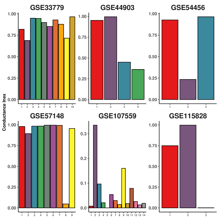
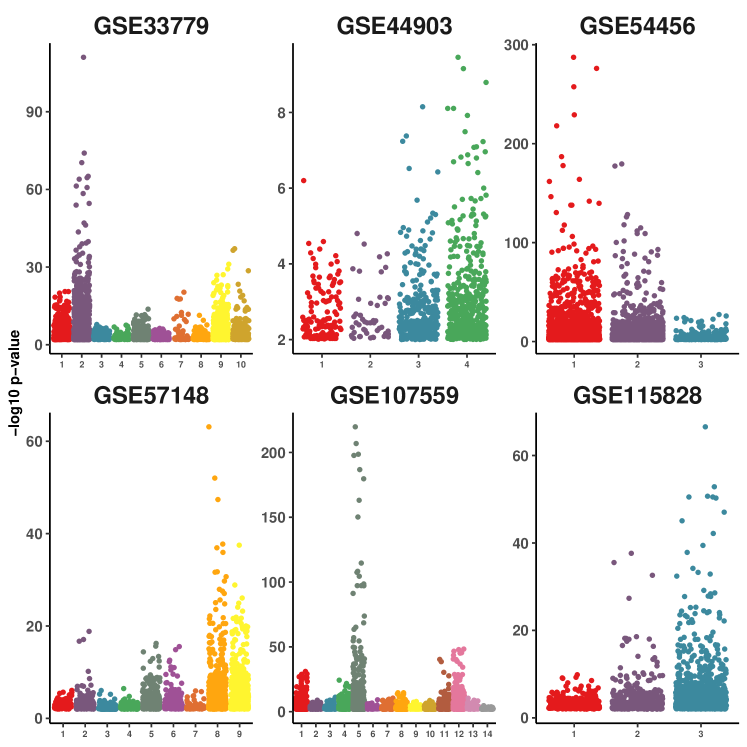
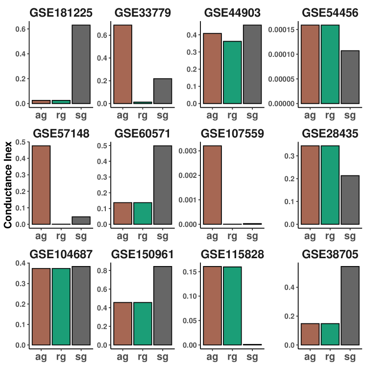
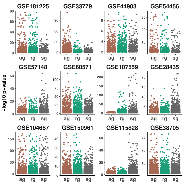
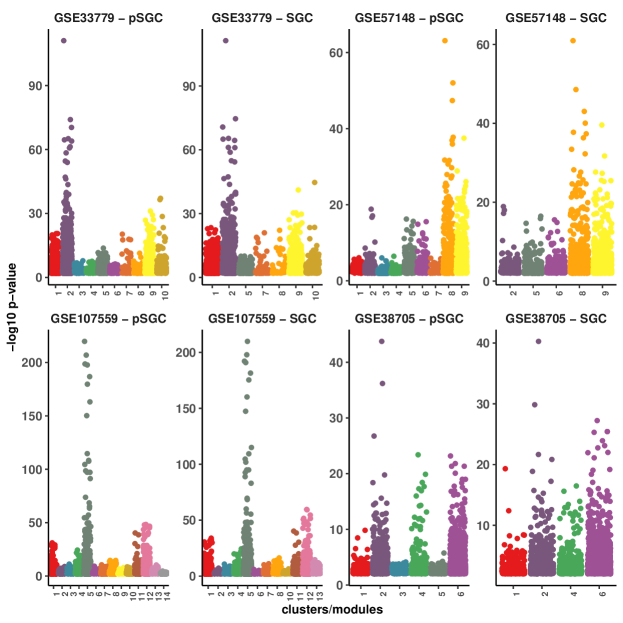
Several unsupervised clustering algorithms have been used for gene expression data [Daxin2004]; among them hierarchical, partitioning, and model-based methods are widely being used in GCNs [Sipko2017, Oyelade2016, D'haeseleer2005, Gibbons2002]. The three pipelines in the benchmark use “Dynamic Tree Cut” R-package for the unsupervised step [dynamicTreeCut] which is a variant of hierarchical clustering (HC) [D'haeseleer2005, Oyelade2016, Gibbons2002]. While in SGC, the kmeans partitioning algorithm [KMeans] is the main method for clustering, and it produces the initial clusters. The gene cluster assignment may change later during the Gene Semi-labeling and Semi-supervised Classification steps as the final modules are produced. In all expression dataset, all the three frameworks in the benchmark have produced relatively more modules but smaller in size in compare with pSGC, and SGC (see Table 1). The maximum number of clusters for WGCNA, CoExpNets, and CEMiTool are , , and that happened in four data, while the corresponding number of clusters in for pSGC and SGC are , , , indicating that SGC treats the network completely different than WGCNA. This smaller number of clusters makes kmeans to be an appropriate choice of clustering since it is shown that the enrichment of the cluster tend to be higher at lower number of clusters [Gibbons2002]. In fact, other advantages of kmeans makes superior solution for unsupervised method. In kmeans, the assignment of the genes to modules reexamined for multiple time based on the information of the gene to the centroids. Whereas, in HC the assignment of genes to a module examines only for one time based on local information of the genes’ pairwise distance [Oyelade2016]. Although both kmeans and HC are sensitive to outliers [D'haeseleer2005, Gibbons2002, Oyelade2016], the embedding the data into new dimensions prior to kmeans helps SGC to be more robust to noise. This embedding along with the approach to pick also helps kmeans algorithm to be more robust with number of cluster . In general, kmeans is sensitive to , and different number of cluster may result in completely different clusters in shape and size [Gibbons2002, D'haeseleer2005, Oyelade2016]. In order to address this concern, in SGC, three methods are examined to pick ; additive gap , relative, and second-order gap. For each method the information of cluster conductance index [conductance] along with GO enrichment [Khatri2005] are used to make decision on final . This helps to select based on more global information. More precisely, we found out for , there is correspondence between clusters’ enrichment and conductance indices such that clusters with lower conductance indices tends to be more enriched in each method. In Figure 2 the conductance indices of the clusters along with their corresponding enrichment is depicted for data whose larger than . Note that this is the result of the clustering for the selected method. As it seen, in all data except GSE54456, clusters with smaller conductance indices have higher enrichment. Intuitively, this is plausible, as the kmeans on the embedding data tries to minimize the conductance index, and as this index gets smaller, clusters become more well-formed. In GSE107559 the smaller conductance indices happened in clusters with label [Yiannis] : Label numbers are arbitrary, a side-effect of the numbering of the genes, so this does not make much sense (see 2(a)). Interestingly, from 2(b), it can be seen that these clusters have higher enrichment. Once the cluster with minimum conductance index is selected for the methods individually, the GO enrichment over those selected clusters will finalize the selected . Figure 3 shows the minimum cluster conductance for the three methods, along with their corresponding enrichment. ag, rg, and sg denote additive gap, relative gap, and second-order gap methods. We found that in data, clusters with smaller conductance index tend to have higher enrichment, while it is not hold for other data. Therefore, it is reasonable to finalized the method based on the enrichment of these clusters. Finally, On the benchmark data, we discovered that this approach for picking works well for all except one (GSE44903).
Once modules are produced, GO enrichment analysis is applied for cluster quality. This technique is the most well-grounded measure for module evaluation and it uses the GO information [Rhee2008]. Statistically, in a given module, this method determines the significance of the GO terms for a test query by associating p-values . The query includes the test direction, either “underrepresented” (under) or “overrepresented” (over), and three ontologies; “biological process” (BP), “cellular component” (CC), and “molecular function” (MF). p-values are derived based on the number of observed genes in a specific query with the number of genes that might appear in the same query if a selection performed from the same pool were completely random. In effect, this values identify if the GO terms that appear more frequently than would be expected by chance [Khatri2005]. As usual the smaller the p-value the more significant the GO term. Here, we use GOstats [GOstats] for module enrichment of all the pipelines with the same input parameter settings. To this end, we specified conditional hypergeometric test on all possible of test queries; ‘overBP”, “overCC”, “overMF”, “underBP”, “underCC”, “underMF”. This conditional test is used to reduce the false positive rate and control the type I error that may arise due to hierarchical structure of the GO [Khatri2005, Rhee2008, GOstats]. GOstats performs the analysis based on hypergeometric distribution and it returns the enrichment results for each module on data individually. shows the summary of the result after GO enrichment on the pipelines for the dataset.
While module enrichment for all the frameworks is ready, SGC performs additional steps to give the final modules. For aim of simplicity, we call these steps semi-labeling steps. In semi-labeling steps, the information from GO and the kmeans clusters, from previous steps, are used to determine the remarkable and unremarkable genes. The genes associated to the top of all the GO terms from all modules collectively form the remarkable genes. It is assumed that the label of the remarkable genes is correct ( since they make the module to be highly enriched). Now, remarkable genes along with their labels are fed into a supervised machine learning model as the training set. At this stage the problem is changed to semi-supervised. The model, next, makes prediction for unremarkable genes and assigns new label to them ( see subsection 2.1). This extra step is plausible because it reconsiders the unremarkable genes and tries to assign new label based on what have been observed for GO enrichment on the initial clusters. The new module assignment allows the unremarkable genes to participate into significant GO term. We observed that this step leads to the vanishing the clusters that are not highly enriched. In Table 1 the summary of the semi-labeling steps is given. “%UNR Genes” indicates percentage of the total genes that are unremarkable, and “% CH Label” specifies the percentage of the unremarkable genes that their label have been changed after semi-labeling steps. The small size of unremarkable genes means that the enrichment of all the clusters are similar, and the majority of the genes have contributed in at least one significant GO term. This makes that the semi-labeling modules agree with kmeans clusters. This happens in GSE104687, GSE181225, GSE54456, GSE107559, and GSE150961. On the contrary, in larger unremarkable gene size, SGC assigns new label for unremarkable genes and change the clusters’ shape and size. The highest unremarkable gene size occurred in GSE33779, GSE57148, and GSE38705 and in Figure 4 the difference between enrichment of the clusters and modules this data are shown. As it seen, in all of this data, the number of modules are reduced and the overall modules’ enrichment are increased. Interestingly, despite the fact that in GSE107559 the percentage of the unremarkable genes and changed label relatively is low, and respectively, this little change of gene assignment has wiped out clusters. In general, if the enrichment of the clusters are not similar, semi-labeling steps eliminates the non-enriched clusters. Finally, at the end of this step final modules are ready and GOstats is carried out one more time on them returning the result for module enrichment.
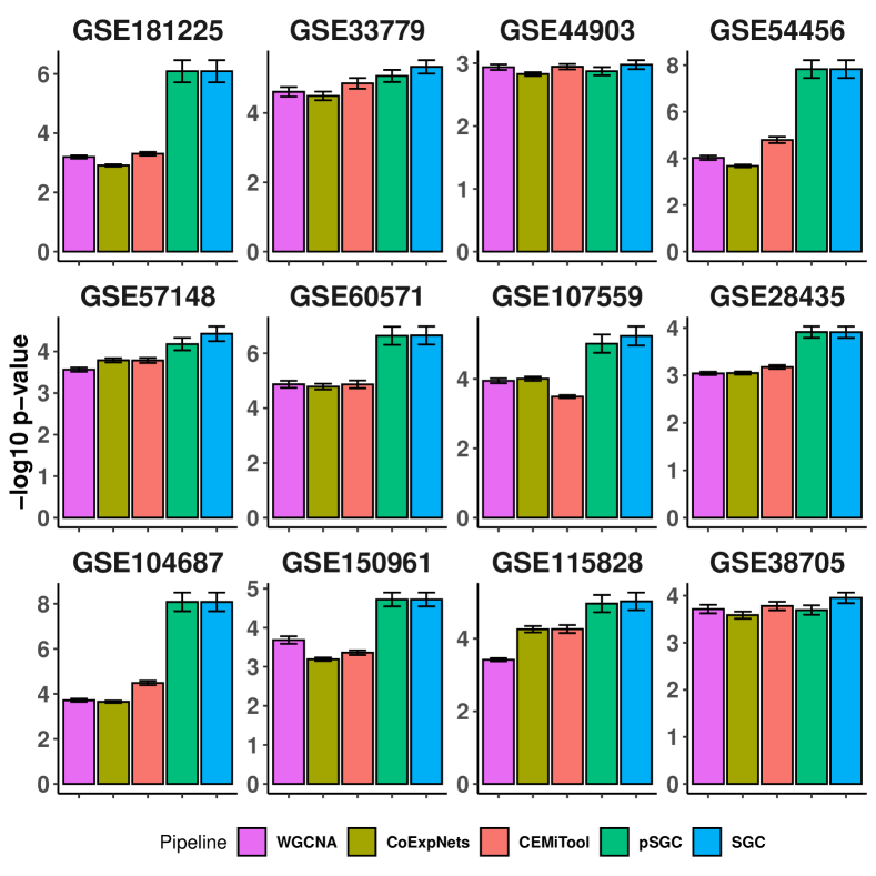
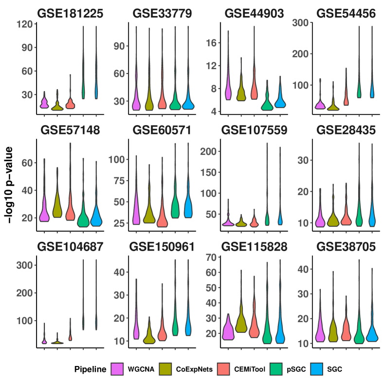
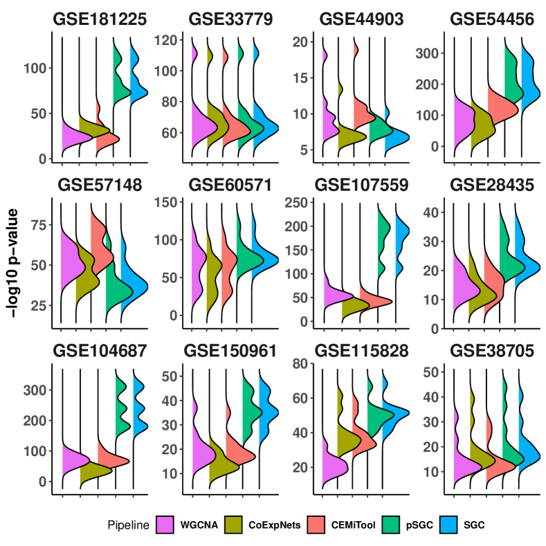
Now, we compare the module enrichment for WGCNA, CoExpNets, CEMiTool, pSGC, and SGC ( Figure 5). Recall that pSGC and SGC denote the clusters and modules respectively. In all gene expression data, pSGC followed by SGC perform better than three tested methods. Following previous convention and methodology [Song2012, CCor2016], we evaluate the performance of the frameworks by comparing the average over the p-values from all the modules collectively. More precisely, let be the th order p-value calculated for module . Then, the quality of module is defines as where is the number of GO terms found in module . Finally, the quality of framework is defines as where is the number of modules in . 5(a) shows the pipeline performance across the benchmark dataset. The higher the bar, the finer the pipeline performance. As it seen, in all the data module quality for pSGC followed by SGC outperforms the other pipeline except GSE44903. This goes to its highest for GSE181225, GSE54456, and GSE104687. As it was expected, for the data that the majority of the genes are remarkable, both pSGC and SGC have similar quality. While, in other cases, SGC improves the quality. In GSE33779, GSE44903, and GSE38705 semi-labeling steps increases the module performance from pSGC to SGC. This causes that SGC surpasses all pipelines in GSE38705. Note that p-values are log-transformed. We then noticed that the main difference between pipeline enrichment is due to the top GO terms. Hence, the top p-values are evaluated as the violin plot. 5(b) compares those points across the pipelines per expression data. The higher the violin, the more significant the GO terms. In all the data, top GO terms in pSGC and SGC is higher than the other frameworks except GSE44903 and GSE57148. It is worth to mention that in GSE57148, CEMiTool is the only framework that surpass pSGC and SGC, and the enrichment of these two frameworks is still higher than the rest of methods. We say, method is dominant to method if the majority of GO terms in is higher than . As it seen, in data (GSE181225, GSE54456, GSE107559, GSE28435, GSE104687), pSGC and SGC are dominant to others. Pipelines almost behave similar in GSE33779 and GSE38705. In other data still ( GSE150961, GSE11582, GSE60571, and GSE38705) the violin for pSGC and SGC tends to be higher in compare with the other three methods. Next, we dive into prominent modules. We say, module in pipeline is prominent if the most significant p-value in is more significant than other all p-values in other modules of . In next effort, the distribution of the top GO terms in prominent module of each framework is illustrated for the all GE data individually. 5(c) shows the result. As usual, the higher the density the more significant the p-values. The GO terms found in prominent module of pSGC and SGC is higher than the three other methods except in GSE44903 and GSE57148. Similar to 5(b), in GSE57148, CEMiTool only performs better than pSGC and SGC. Similar to 5(b) in dataset, pSGC and SGC are dominant to others astonishingly. In two data, the pipeline almost have similar enrichment, and in rest of the data, they still perform better than the three tested framework. This result suggests that pSGC clusters and SGC modules are more enriched in compare with WGCNA, CoExpNets, and CEMiTool. Specially we found out for the top GO terms, that make differences in enrichment, modules of pSGC and SGC are noticeably more significant in compare with other three tested methods.
GOstats, also returns the odds ratio value associated to each GO term. The odds ratio was defined as the proportion of a GO term genes within a module to the proportion of this GO term genes in the dataset. More precisely, it evaluates strength of the GO term within a module [MOET]. As usual, the higher the odds ratio, the more stronger the enrichment. Here, the odds values are discretized into four bins; 0, less equal to 1 ( ), greater than 1 ( ), and infinity . The percentage of the GO terms that their corresponding odds ratio fall in each bin was calculated for each pipeline on the data individually. 5(d) shows the results. The zero odds ratio occurs if none of the GO term genes in the data fall in the module, however, the p-value of the term is significant. All pipelines have almost similar percentage for zero odds ratio except GSE60571, and GSE115828 in which pSGC and SGC have less number of GO terms for this bin. And, this is revers for GSE181225. The red stack shows the proportion of the GO terms that have odds ratios less or equal to . Almost in all the cases pSGC and SGC have more percentage in compare with the other three frameworks. Similarly, the green stack indicates the proportion of GO term that they corresponding odds ratio is greater than . As it seen, other pipelines than pSGC, and SGC have larger portion for this bin. Finally, the orange stack indicate the positive infinity odds ratios. The infinity odds ratio occurs if all the genes associated to a GO term in the dataset fall in a same module. This happens the largest for GSE181225 in case of WGCNA, CoExpNets, and CEMiTool. And GSE54456, GSE57148, GSE104687, GSE107559 for pSGC, SGC. Interestingly, in these data pSGC and SGC are dominant to the rest except GSE57148.
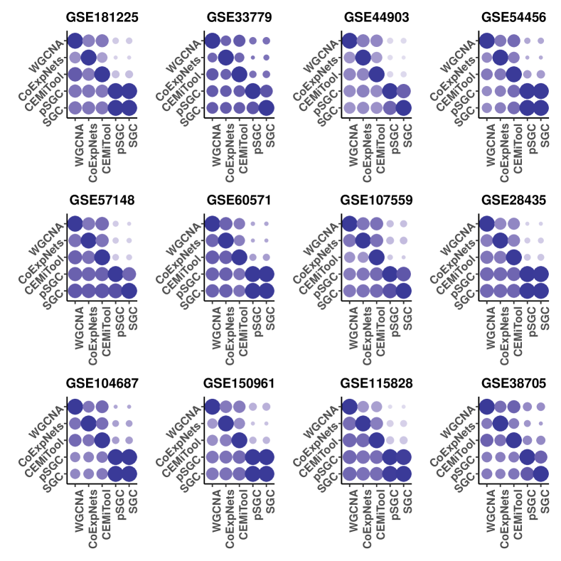
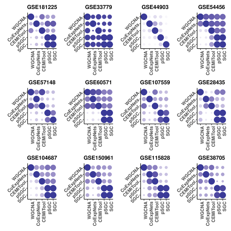
It is interesting to investigate the overlapping GO terms among the pipelines. In Figure 6 we explored this in two scenarios; among all GO terms collectively, and among prominent modules. The bigger and darker a circle the higher the percentage. In the former scenario, the percentage is consider for all GO terms found in all modules of a pipeline. The overlapping percentage method with respect to method is calculated as where is the number of common terms between and and is the number of GO terms found in and it is shown for and in x and y axis in 6(a). As it was expected, pSGC and SGC have higher percentage with each other in compare with other pipelines. While, other methods have higher percentage among themselves. This is not surprising as these methods share fundamental steps. In the later scenario, the overlapping percentage is considered among the prominent modules. Let and denote the prominent module in and respectively. The percentage for with respect to is calculated as where is the number of common terms between and and is the number of terms in and is depicted for and in x and y axis in 6(b). As it seen, while in this scenario pSGC and SGC share higher percentage with respect to other pipelines, the reverse is not observed and it happens to its highest in GSE54456 followed by GSE60571 and GSE104687. In GSE33779 all the pipelines except CEMiTool share significant percentages.
We have proposed a comprehensive pipeline for gene co-expression networks which utilizes the self-training approach for converting the problem into semi-supervised. Our pipeline overcomes the bottlenecks of the existing approaches and, in an innovative fashion, integrates geometric similarity measure, gene ontology information, kmeans clustering, and spectral graph theory knowledge to produce more enriched modules. Existing pipelines mainly use Pearson correlation (PC) as the similarity metric. While this has been controversial as the expression values are positive and there is not clear interpretation of the negative coefficients. Additionally, PC is unable to capture the non-linear dependencies within the genes [niloo2021]. Recently, it has been shown that Pearson correlation is not appropriate metric for gene expression clustering [Pearson]. In addition to PC, the scale-free criteria of biological network is another constraint that it has been is widely practiced in GCNs [Zhang2005general, Lan2008, Botia2017, Russo2018]. A network is scale-free if its node degree is proportional to power-law degree [Clote2020]. While many pipelines rely on this assumption [Zhang2005general, Lan2008, Botia2017, Russo2018, petal2015], this concept is questioned by multiple studies [SChaefer2017]. More precisely, extensive research have shown that most of biological networks are not subject to scale-freeness criteria [Raya2006, Lima2009, Broido2019, Clote2020]. Throughout are experiments we observed that powering the adjacency matrix, in general, lead to more module enrichment. Previously, it is discussed that Euclidean distance is an appropriate choice for gene expression [D'haeseleer2005, Gibbons2002]. Hence, we utilized Gaussian kernel function as the main core for the similarity metric. This is a geometric measure that inherently powers the Euclidean coefficient and it ranges positively from as the most dissimilar to as the most similar.
As we discussed earlier, while properties of hierarchical clustering make it inferior to other approaches, classical approach in GCNs heavily rely on Hierarchical clustering (HC) to find modules [dynamicTreeCut]. It is also shown that HC perform worse than if genes were assigned to modules randomly and kmeans achieve a better result for gene expression data [D'haeseleer2005, Gibbons2002, Daxin2004, Oyelade2016]. Here, we deviate from HC and use Spectral clustering (i.e. data embedding followed by kmeans) as the main method for unsupervised step. The embedding data causes kmeans to be more robust to outliers. More importantly, classical approaches including HC utilize topological evaluation in order to find an optimal number of clusters , while in SGC three different potential are evaluated both internally and externally using conductance index [conductance] and GO enrichment [Khatri2005] combine. This is appropriate as kmeans is sensitive to , and enables it to pick based on more comprehensive information. We consider conductance index as the internal cluster evaluation because spectral clustering tries to minimizes the conductance index [conductance].
In effect, we observed that there is correspondence between the cluster conductance index and cluster enrichment, as the conductance index tend to be smaller, the cluster enrichment tends to be higher. Intuitively, this is reasonable as the spectral clustering (i.e. embedding followed by kmeans) tries to minimizes the conductance index. As a result, it is expected to see higher enrichment in well-formed clusters. We observed that in all the cases except one the better choice of was selected.
In addition, while classical approaches employ GO enrichment for module quality, we utilize this information inside the pipeline. The main target in GCNs is to return highly enriched modules, and therefore genes that cause the high enrichment are assigned correctly (i.e. remarkable genes), while the remaining genes need to reexamine (i.e. remarkable genes). So far, we have evident that gene expression data couple with kmeans were not able to make good assignment for unremarkable genes. As a result, these genes are allowed to review thoroughly using the transformed data, kmeans, and GO enrichment information. We have observed that this lead to eliminate the non-enriched module and increase the overall module enrichment.
2.1 Online Methods
SGC framework. SGC framework is developed for GCNs construction and analysis. It takes the gene expression (GE) dataset as the input. It then clusters the genes so that the genes that fall within the same cluster have a similar expression pattern. To stick with the machine learning convention, SGC takes an expression matrix, , as the input in which rows and columns correspond to genes and samples respectively. Each entry is an expression value gene in sample . SGC does not perform any normalization or correction for batch effects and it is assumed that these preprocessing step is already performed. SGC is based on master steps. The parameter in each step can be adjusted by the user.
2.1.1 Network Construction
2.1.1.1 Normalization
In this step, each vector of gene in the expression matrix is divided by its Euclidean norm which is calculated by Equation 1
| (1) |
Where is the expression vector of gene . The result of this step is matrix which has the same dimensions as .
2.1.1.2 Similarity Calculation
Gaussian kernel function, , is the main function that is used to compute the gene pairwise associations. This function takes from previous step and calculates the similarity values using Equation 2 where is the variance over the all the pairwise Euclidean norm (Equation 1) among the genes. The result is a similarity matrix where is the number of the genes. Note that is a symmetric square matrix which ranges from for the most dissimilar to for the most similar genes.
| (2) |
2.1.1.3 TOM Addition
The adjacency of the network is then derived by adding the information of the second-order of the neighborhood to in the form of the topological overlap measure (TOM) [Zhang2005general, Lan2008]. Equation 3 gives its formula
| (3) |
where , and is the similarity coefficient between gene and from matrix of previous step, and is the degree of node (which is the sum of the similarity values from node to and all its neighbors).
We also propose a novel measure call Deep Overlap Measure (DOM). Similar to TOM, DOM captures and adds the information of third order neighborhoods of the genes to the network in form of Equation 4
| (4) |
where , and . There rest of parameters are the same as TOM (i.e. Equation 3). By default, SGC calculates TOM, however, users can specify DOM by setting flagDOM = TRUE.
The result of this step, is a squared symmetric adjacency matrix with values in where is the number of genes. Note that diagonal elements of is zero.
2.1.2 Network Clustering
2.1.2.1 Transformation
Given the adjacency matrix , in this step firstly the eigenvalues and eigenvectors of the associated graph Laplacian are calculates where is the diagonal matrix in which each diagonal entry denotes the degree node in . Let and denote the these eigenvalues and eigenvectors respectively, and assume is a vector in which each entry denotes the degree node from . Then the following steps are taken in order.
-
I
.
-
II
where is the transpose of vector .
-
III
where and is the division of every element in by .
-
IV
where , for every column in .
The result is a squared matrix where is the number of the genes. Since the first eigenvalue of a symmetric squared matrix is always , the corresponding column in is dropped resulting in matrix .
2.1.2.2 Number of Clusters
Three methods are proposed to find the optimal number of clusters all based on eigenvalues derived from previous step; additive gap, relative gap, and the second-order Gap.
Suppose are the eigenvalues. The following quantities are calculated.
| (5) |
| (6) |
| (7) |
Then, the number of clusters in additive gap, relative gap and second-order gap are as follow.
| (8) |
| (9) |
| (10) |
And , , and denote the number of clusters for methods additive gap, relative gap, and second-order gap respectively. Note that is dropped since the first eigenvalue in is always .
2.1.2.3 Calculation of Conductance Index
For each number of cluster , is considered as the first columns (i.e. eigenvectors) of . Each row in is then divided by its Euclidean norm Equation 1 so that length of each row becomes . Next, kmeans clustering algorithm [KMeans] is applied on to find cluster using the default kmeans() R function. By default, the maximum number of iterations is set to and the number of starts is set to . Now, for each cluster the conductance index is computed. Let is one of the clusters. Then, the conductance index for cluster is calculated by Equation 11
| (11) |
Where which indicates the degree node (sum of all the weights associated to node ), and is the pairwise association between node and in adjacency matrix . For each method, the cluster that has the minimum conductance index is chosen and passed to the next level. Let , , and denote the cluster with minimum conductance index for gap, first, and second methods respectively.
2.1.2.4 Gene Ontology Cross Validation
In this step, the enrichment of , , and are calculated using GOstats [GOstats] R package individually for all six possible queries (i.e. “underBP”, “overBP”, “underCC”, “overCC”, “underMF”, “overMF‘”) combine. To this end, a conditional “hyperGTest” function is performed and the entire genes in the data is considered for the “universeGeneIds”. For each cluster , it returns an information of the significant GO terms found in by associating p-values to the terms. Let denote the p-value associated to a GO term found in . Then the optimal method is determined as follow
| (12) |
Let is the cluster number correspond to winner method . At the end of this step, the clusters produced by method along with embedded matrix (the first columns of ) is passed to the next step.
2.1.3 Gene Ontology
In the gene ontology (GO) step, the GOstats R package [GOstats] with same setting as before is applied on the clusters derived from previous step individually. GOstats return the information of the significant GO terms found for each query in the clusters. This includes “id”, “term”, “p-value”, “odds” “ratio”, “expected count”, “count”, “size”. In SGC the information for each query are combined and returns for the clusters separately. Additionally, for each cluster , the genes associated to each GO term that have been found in also is returned.
2.1.4 Semi-Labeling
In this step, for each cluster the remarkable GO terms and consequently remarkable genes are determined. A GO term is remarkable if its corresponding p-value is less than a cutoff, and accordingly, the genes associated to that GO term are remarkable genes. Remarkable genes within a cluster are labeled as . In other words, If any gene in belongs to a GO term which is more significant than a cutoff, then the will be labeled as otherwise it is unlabeled, or its label is not determined yet. This process is performed for all the clusters, and genes belong to GO terms more significant than the cutoff are labeled corresponding to their cluster labels. By default, cutoff is considered as the quantile over all p-values found in all clusters collectively. However, this quantile is adjustable to users.
2.1.5 Semi-Supervised Classification
Labeled and unlabeled gene sets along with their corresponding vector in (from Network clustering) are fed to a supervised model; either k-nearest neighbors (kNN) supervised machine learning algorithm [knn1, knn2] or logistic regression [lr]. The model is called semi-supervised since all the datapoints are not labeled, and it makes prediction of unlabeled genes on the basis of the labeled one. Note that for each gene, the length of its corresponding vector is where is the optimal number of cluster found in step Network Clustering. After this step, genes that belong to the same class form a module and number of modules are equal to number of clusters that remarkable at least one GO term has been found in it. The default model is kNN and its hyper-parameter by default is if otherwise . Final supervised model is determined by cross validation on accuracy metric using [caret] R-package.
Finally, a brief word of caution is necessary. So far, the steps proposed in SGC are a general steps that we found out it works well in most of the cases. However, it is highly recommended to see the different setting. As an example, we found that if other method was used for GSE44903, SGC will outperform the rest significantly. Fortunately, SGC enables user to change the configuration easily.
2.2 Pipelines
As it discussed earlier, all the pipeline in the benchmark use soft-power (sft) to make the GCNs scale-free. For each data, same soft-power is used for scale-free constraint and is written in Table 1. Function “blockwiseModules” is used for “signed” GCNs construction and produce modules for WGCNA. Function “getDownstreamNetwork” is used for “signed” GCNs construction and analysis in CoExpNets. Finally, “cemitool” function is used to build “signed” GCNs construction and produce modules for CEMiTool framework.
3 Supplementary Files
Suppl