Cross Project Software Vulnerability Detection via Domain Adaptation and Max-Margin Principle

Abstract

Software vulnerabilities (SVs) have become a common, serious and crucial concern due to the ubiquity of computer software. Many machine learning-based approaches have been proposed to solve the software vulnerability detection (SVD) problem. However, there are still two open and significant issues for SVD in terms of i) learning automatic representations to improve the predictive performance of SVD, and ii) tackling the scarcity of labeled vulnerabilities datasets that conventionally need laborious labeling effort by experts. In this paper, we propose a novel end-to-end approach to tackle these two crucial issues. We first exploit the automatic representation learning with deep domain adaptation for software vulnerability detection. We then propose a novel cross-domain kernel classifier leveraging the max-margin principle to significantly improve the transfer learning process of software vulnerabilities from labeled projects into unlabeled ones. The experimental results on real-world software datasets show the superiority of our proposed method over state-of-the-art baselines. In short, our method obtains a higher performance on F1-measure, the most important measure in SVD, from 1.83% to 6.25% compared to the second highest method in the used datasets. Our released source code samples are publicly available at https://github.com/vannguyennd/dam2p.

Introduction

Software vulnerabilities (SVs), defined as specific flaws or oversights in software programs allowing attackers to exploit the code base and potentially undertake dangerous activities (e.g., exposing or altering sensitive information, disrupting, degrading or destroying a system, or taking control of a program or computer system) (Dowd, McDonald, and Schuh 2006), are very common and represent major security risks due to the ubiquity of computer software. Detecting and eliminating software vulnerabilities are hard as software development technologies and methodologies vary significantly between projects and products. The severity of the threat imposed by software vulnerabilities (SVs) has significantly increased over the years causing significant damages to companies and individuals. The worsening software vulnerability situation has necessitated the development of automated advanced approaches and tools that can efficiently and effectively detect SVs with a minimal level of human intervention. To respond to this demand, many vulnerability detection systems and methods, ranging from open source to commercial tools, and from manual to automatic methods (Neuhaus et al. 2007; Shin et al. 2011; Yamaguchi, Lindner, and Rieck 2011; Grieco et al. 2016; Li et al. 2016; Kim et al. 2017; Li et al. 2018b; Duan et al. 2019; Cheng et al. 2019; Zhuang et al. 2020) have been proposed and implemented.

Most previous work in software vulnerability detection (SVD)(Neuhaus et al. 2007; Shin et al. 2011; Yamaguchi, Lindner, and Rieck 2011; Li et al. 2016; Grieco et al. 2016; Kim et al. 2017) has based primarily on handcrafted features which are manually chosen by knowledgeable domain experts with possibly outdated experience and underlying biases. In many situations, these handcrafted features do not generalize well. For example, features that work well in a certain software project may not perform well in other projects (Zimmermann et al. 2009). To alleviate the dependency on handcrafted features, the use of automatic features in SVD has been studied recently (Li et al. 2018b; Lin et al. 2018; Dam et al. 2018; Li et al. 2018a; Duan et al. 2019; Cheng et al. 2019; Zhuang et al. 2020). These works show the advantages of employing automatic features over handcrafted features for software vulnerability detection.

Another major challenging issue in SVD research is the scarcity of labeled software projects to train models. The process of labeling vulnerable source code is tedious, time-consuming, error-prone, and can be very challenging even for domain experts. This has resulted in few labeled projects compared with a vast volume of unlabeled ones. Some recent approaches (Nguyen et al. 2019, 2020; Liu et al. 2020) have been proposed to solve this challenging problem with the aim to transfer the learning of vulnerabilities from labeled source domains to unlabeled target domains. Particularly, the methods in Nguyen et al. (2019, 2020) learn domain-invariant features from the source code data of the source and target domains by using the adversarial learning framework such as Generative Adversarial Network (GAN) (Goodfellow et al. 2014) while the method in Liu et al. (2020) consists of many subsequent stages: i) pre-training a deep feature model for learning representation of token sequences (i.e., source code data), ii) learning cross-domain representations using a transformation to project token sequence embeddings from (i) to a latent space, and iii) training a classifier from the representations of the source domain data obtained from (ii). However, none of these methods exploit the imbalanced nature of source code projects for which the vulnerable data points are significantly minor comparing to non-vulnerable ones.

On the other side, kernel methods are well-known for their ability to deal with imbalanced datasets (Schölkopf et al. 2001; Tax and Duin 2004; Tsang et al. 2005; Tsang, Kocsor, and Kwok 2007; Le et al. 2010; Nguyen et al. 2014). In a nutshell, a domain of majority, which is often a simple geometric shape in a feature space (e.g., half-hyperplane (Schölkopf et al. 2001; Nguyen et al. 2014) or hypersphere (Tax and Duin 2004; Tsang et al. 2005; Tsang, Kocsor, and Kwok 2007; Le et al. 2010) is defined to characterize the majority class (i.e., non-vulnerable data). The key idea is that a simple domain of majority in the feature space, when being mapped back to the input space, forms a set of contours which can distinguish majority data from minority data.

In this paper, by leveraging learning domain-invariant features and kernel methods with the max-margin principle, we propose Domain Adaptation with Max-Margin Principle (DAM2P) to efficiently transfer learning from imbalanced labeled source domains to imbalanced unlabeled target domains. Particularly, inspired by the max-margin principle proven efficiently and effectively for learning from imbalanced data, when learning domain-invariant features, we propose to learn a max-margin hyperplane on the feature space to separate vulnerable and non-vulnerable data. More specifically, we combine labeled source domain data and unlabeled target domain data, and then learn a hyperplane to separate source domain non-vulnerable from vulnerable data and target domain data from the origin such that the margin is maximized. In addition, the margin is defined as the minimization of the source domain and target domain margins in which the source domain margin is regarded as the minimal distance from vulnerable data points to hyperplane (Nguyen et al. 2014), while the target domain margin is regarded as the distance from the origin to the hyperplane (Schölkopf et al. 2001).

Our contributions can be summarized as follows:

• We leverage learning domain-invariant features and kernel methods with the max-margin principle to propose a novel approach named DAM2P that can bridge the gap between the source and target domains on a joint space while being able to tackle efficiently and effectively the imbalanced nature of the source and target domains to significantly improve the transfer learning process of SVs from labeled projects into unlabeled ones.

• We conduct extensive experiments on real-world software datasets consisting of FFmpeg, LibTIFF, LibPNG, VLC, and Pidgin software projects. It is worth noting that to demonstrate and compare the capability of our proposed method and baselines in the transfer learning for SVD, the datasets (FFmpeg, VLC, and Pidgin) from the multimedia application domain are used as the source domains whilst the datasets (LibPNG and LibTIFF) from the image application domain were used as the target domains. The experimental results show that our method significantly outperforms the baselines by a wide margin, especially for the F1-measure, the most important measure used in SVD problems.

Related Work

Automatic features in software vulnerability detection (SVD) has been widely studied (Li et al. 2018b; Lin et al. 2018; Dam et al. 2018; Li et al. 2018a; Duan et al. 2019; Cheng et al. 2019; Zhuang et al. 2020) due to its advantages of employing automatic features over handcrafted features. In particular, Dam et al. (2018) employed a deep neural network to transform sequences of code tokens to vectorial features that are further fed to a separate classifier; whereas Li et al. (2018b) combined the learning of the vector representation and the training of the classifier in a deep network. Advanced deep net architectures have been investigated for SVD problem. Russell et al. (2018) combined both recurrent neural networks (RNNs) and convolutional neural networks (CNNs) for feature extraction from the embedded source code representations while Zhuang et al. (2020) proposed a new model for smart contract vulnerability detection based on a graph neural network (GNN) (Kipf and Welling 2016).

Deep domain adaptation-based methods have been recently studied for cross-domain SVD. Notably, Nguyen et al. (2019) proposed a novel architecture and employed the adversarial learning framework (e.g., GAN) to learn domain-invariant features that can be transferred from labeled source to unlabeled target code project. Nguyen et al. (2020) enhanced Nguyen et al. (2019) by proposing an elegant workaround to combat the mode collapsing problem possibly faced in that work due to the use of GAN. Finally, Liu et al. (2020) proposed a multi-stage approach with three sequential stages: i) pre-training a deep model for learning representation of token sequences (i.e., source code data), ii) learning cross-domain representations using a transformation to project token sequence embeddings from (i) to a latent space, iii) training a classifier from the representations of the source domain data obtained from (ii). The trained classifier is then applied to the target domain.

In computer vision, deep domain adaptation (DA) has been intensively studied and shown appealing performance in various transfer learning tasks and applications, notably DDAN (Ganin and Lempitsky 2015), MMD (Long et al. 2015), D2GAN (Nguyen et al. 2017), DIRT-T (Shu et al. 2018), HoMM (Chen et al. 2020), and LAMDA (Le et al. 2021). Most of the introduced methods were claimed, applied and showed the results for vision data. There is no evidence that they can straightforwardly be applied for sequential data such as in cross-domain SVD. In our paper, inspired from Nguyen et al. (2019), we borrowed the principles of some well-known and state-of-the-art methods, e.g., DDAN, MMD, D2GAN, DIRT-T, HoMM and LAMDA, and refactored them using the CDAN architecture introduced in Nguyen et al. (2019) for cross-domain SVD to compare with our proposed approach.

Domain Adaptation with Max-Margin Principle

Problem Formulation

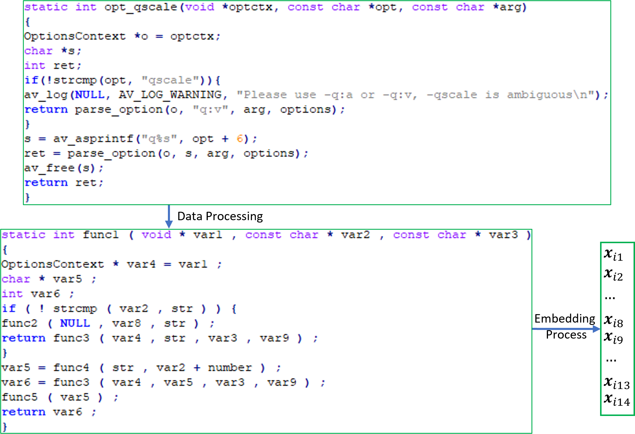
Given a labeled source domain dataset $S=\left\{\left(\boldsymbol{x}_{1}^{S},y_{1}\right),\dots,\left(\boldsymbol{x}_{N_{S}}^{S},y_{N_{S}}\right)\right\}$ where $y_{i}\in\left\{0,1\right\}$ (i.e., $1$: vulnerable code and $0$: non-vulnerable code), let $\boldsymbol{x}_{i}^{S}=\left[\boldsymbol{x}_{i1}^{S},\dots,\boldsymbol{x}_{iL}^{S}\right]$ be a code function represented as a sequence of $L$ embedding vectors. We note that each embedding vector corresponds to a statement in the code function. Similarly, the unlabeled target domain dataset $T=\left\{\boldsymbol{x}_{1}^{T},\dots,\boldsymbol{x}_{N_{T}}^{T}\right\}$ consists of many code functions where each code function $\boldsymbol{x}_{i}^{T}=\left[\boldsymbol{x}_{i1}^{T},\dots,\boldsymbol{x}_{iL}^{T}\right]$ is a sequence of $L$ embedding vectors.

Figure 4 shows an example of the overall procedure for the source code data processing and embedding (please refer to the appendix for details).

Figure 1: An example of the overall procedure for data processing and embedding of a source code function. After the data processing step (e.g., removing comments and non-ASCII characters), we use the embedding process to obtain the embedded vectors for the source code statements.

In standard DA approaches, domain-invariant features are learned on a joint space so that a classifier mainly trained based on labeled source domain data can be transferred to predict well unlabeled target domain data. The classifiers of interest are usually deep nets conducted on top of domain-invariant features. In this work, by leveraging the kernel theory and the max-margin principle, we consider a kernel machine on top of domain-invariant features, which is a hyperplane on a feature space via a feature map $\phi$.

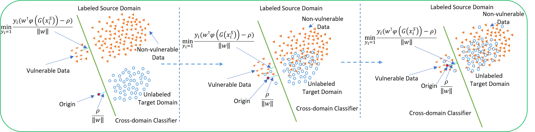
Inspired by the max-margin principle proven efficiency and effectiveness for learning from imbalanced data, when learning domain-invariant features, we propose to learn a max-margin hyperplane on the feature space to separate vulnerable and non-vulnerable code data. More specifically, we combine labeled source domain data and unlabeled target domain data, and then learn a hyperplane to separate source domain non-vulnerable from vulnerable data and target domain data from the origin such that the margin is maximized. Here, the margin is defined as the minimization of the source domain and target domain margins in which the source domain margin is defined as the minimum distance from vulnerable data points to hyperplane (Nguyen et al. 2014) while the target domain margin is defined as the distance from the origin to the hyperplane (Schölkopf et al. 2001).

Our Proposed Approach DAM2P

Domain Adaptation for Domain-Invariant Features

In what follows, we present the architecture of the generator $G$ and how to use an adversarial learning framework such as GAN (Goodfellow et al. 2014) to learn domain-invariant features in a joint latent space specified by $G$. To learn the automatic features for the sequential source code data, inspired by Li et al. (2018b); Nguyen et al. (2019, 2020), we apply a bidirectional recurrent neural network (bidirectional RNN) to both the source and target domains. Given a source code function $\boldsymbol{x}$ in the source domain or the target domain, we denote the output of the bidirectional RNN by $\mathcal{B}\left(\boldsymbol{x}\right)$. We then use some fully connected layers to connect the output layer of the bidirectional RNN with the joint feature layer wherein we bridge the gap between the source and target domains. The generator is consequently the composition of the bidirectional RNN and the fully connected layers: $G\left(\boldsymbol{x}\right)=f\left(\mathcal{B}\left(\boldsymbol{x}\right)\right)$ where $f\left(\cdot\right)$ represents the map formed by the fully connected layers.

Subsequently, to bridge the gap between the source and target domains in the latent space, inspired by GAN (Goodfellow et al. 2014), we use a domain discriminator $D$ to discriminate the source domain and target domain data and train the generator $G$ to fool the discriminator $D$ by making the source domain and target domain data indistinguishable in the latent space. The relevant objective function is hence as follows:

$$\mathcal{H}\left(G,D\right):= \frac{1}{N_{S}}\sum_{i=1}^{N_{S}}\log D\left(G\left(\boldsymbol{x}_{i}^{S}\right)\right)$$

$$+ \frac{1}{N_{T}}\sum_{i=1}^{N_{T}}\log\left[1-D\left(G\left(\boldsymbol{x}_{i}^{T}\right)\right)\right]$$ (1)

where we seek the optimal generator $G^{*}$ and the domain discriminator $D^{*}$ by solving:

$$G^{*}=\underset{{}_{G}}{\text{argmin}\ }\mathcal{H}\left(G,D\right)\,\text{and}\,D^{*}=\underset{{}_{D}}{\text{argmax}}\,\mathcal{H}\left(G,D\right)$$

Cross-domain kernel classifier

To build up an efficient domain adaptation approach for source code data which can tackle well the imbalanced nature of source code projects, we leverage learning domain-invariant features with the max-margin principle in the context of kernel machines to propose a novel cross-domain kernel classifier named DAM2P. We construct a hyperplane on the feature space: $\mathbf{w}^{T}\phi(G(\boldsymbol{x}))-\rho=0$ with the feature map $\phi$ and learn this hyperplane using the max-margin principle. More specifically, we combine labeled source domain and unlabeled target domain data, and then learn a hyperplane to separate source domain non-vulnerable from vulnerable data and target domain data from the origin in such a way that the margin is maximized.

It is worth noting that in this work, the margin is defined as the minimization of the source and target margins in which the source margin is the minimal distance from the source domain vulnerable data points to the hyperplane (Nguyen et al. 2014), while the target margin is the distance from the origin to the hyperplane (Schölkopf et al. 2001). The overall architecture of our proposed cross-domain kernel classifier in the feature space is depicted in Figure 2.

Figure 2: The architecture of our cross-domain kernel classifier in the feature space. By using our DAM2P method, we can gradually bridge the gap between the source and target domains in the latent space, while in the feature space our cross-domain kernel classifier helps to distinguish the vulnerable and non-vulnerable data. At the end, when the source and target domains are intermingled, we can transfer our trained cross-domain kernel classifier to classify the data of the target domain.

Given the source domain dataset $S=\{(\boldsymbol{x}_{1}^{S},y_{1}),\dots,(\boldsymbol{x}_{N_{S}}^{S},y_{N_{S}})\}$ where $y_{i}=1,\,i=1,...,m$ and $y_{i}=0,\,i=m+1,...,N_{S}$ and the target domain dataset $T=\{\boldsymbol{x}_{1}^{T},\dots,\boldsymbol{x}_{N_{T}}^{T}\}$, we formulate the following optimization problem:

$$\underset{\mathbf{w},\rho}{\text{max}}\left(\text{min}\left\{\underset{\text{source margin}}{\underbrace{\underset{y_{i}=1}{\text{min}}\left\{\frac{y_{i}(\mathbf{w}^{\top}\phi(G(\boldsymbol{x}_{i}^{S}))-\rho)}{\left\|\mathbf{w}\right\|}\right\}}},\underset{\text{target margin}}{\underbrace{\frac{\rho}{\left\|\mathbf{w}\right\|}}}\right\}\right)$$ (2)

subject to

$$y_{i}(\mathbf{w}^{\top}\phi(G(\boldsymbol{x}_{i}^{S}))-\rho) \geq 0,\,i=1,...,N_{S}$$

$$\mathbf{w}^{\top}\phi(G(\boldsymbol{x}_{i}^{T}))\geq\rho, \,i=1,...,N_{T}.$$

In the optimization problem (2), $\mathbf{w}$ and $\rho$ are the normal vector and the bias of the hyperplane and $\phi$ is a transformation from the joint latent space to the feature space, while $G$ is the generator used to map the data of source and target domains from the input space into the joint latent space. It occurs that the margin is invariant if we scale $\mathbf{w},\rho$ by a factor $k>0$. Hence without loosing of generality, we can assume that $\text{min}\left\{\underset{y_{i}=1}{\textrm{min}}\left\{y_{i}\mathbf{w}^{\top}\phi(G(\boldsymbol{x}_{i}^{S})-\rho\right\},\rho\right\}=1$. The optimization problem (2) can be rewritten as follows:

$$\underset{w,\rho}{\textrm{min}}\frac{1}{2}\left\|\mathbf{w}\right\|^{2}$$ (3)

subject to

$$\begin{array}[]{l}y_{i}(\mathbf{w}^{\top}\phi(G(\boldsymbol{x}_{i}^{S}))-\rho)\geq 0,\,i=1,...,m\\ y_{i}(\mathbf{w}^{\top}\phi(G(\boldsymbol{x}_{i}^{S}))-\rho)\geq 1,\,i=m+1,...,N_{S}\\ \mathbf{w}^{\top}\phi(G(\boldsymbol{x}_{i}^{T}))\geq\rho,\,i=1,...,N_{T}\end{array}$$

We refer the above model as hard version of our proposed cross-domain kernel classifier. To derive the soft version, we extend the optimization problem in Eq. (3) by using the slack variables as follows:

$$\underset{\mathbf{w},\rho}{\textrm{min}}\left(\frac{1}{2}\left\|\mathbf{w}\right\|^{2}+\frac{1}{N_{S}+N_{T}}\left(\sum_{i=1}^{N_{S}}\xi_{i}^{S}+\lambda\sum_{i=1}^{N_{T}}\xi_{i}^{T}\right)\right)$$ (4)

subject to

$$\begin{array}[]{l}y_{i}(\mathbf{w}^{\top}\phi(G(\boldsymbol{x}_{i}^{S}))-\rho)\geq-\xi_{i}^{S},\,i=1,...,m\\ y_{i}(\mathbf{w}^{\top}\phi(G(\boldsymbol{x}_{i}^{S}))-\rho)\geq 1-\xi_{i}^{S},\,i=m+1,...,N_{S}\\ \mathbf{w}^{\top}\phi(G(\boldsymbol{x}_{i}^{T}))\geq\rho-\xi_{i}^{T},\,i=1,...,N_{T}\\ \xi_{i}^{S}\geq 0,\,i=1,...,N_{S};\xi_{i}^{T}\geq 0,\,i=1,...,N_{T}.\end{array}$$

where $\lambda>0$ is the trade-off hyper-parameter representing the weight of the information from the target domain contributing to the cross-domain kernel classifier.

The primal form of the soft model optimization problem is hence of the following form:

$$\underset{\mathbf{w},\rho}{\text{min}}\mathcal{L}(G,\mathbf{w},\rho)$$ (5)

where we have defined

$$\mathcal{L}(G,\mathbf{w},\rho):= \frac{1}{2}\left\|\mathbf{w}\right\|^{2}+\frac{1}{N_{S}+N_{T}}\underset{i=1}{\overset{m}{\sum}}\max\left\{0,-z_{i}\right\}$$

$$+ \frac{1}{N_{S}+N_{T}}\underset{i=m+1}{\overset{N_{S}}{\sum}}\max\left\{0,-z_{i}+1\right\}$$

$$+ \frac{\lambda}{N_{S}+N_{T}}\underset{i=1}{\overset{N_{T}}{\sum}}\max\left\{0,-\mathbf{w}^{\top}\phi(G(\boldsymbol{x}_{i}^{T}))+\rho\right\}$$

with $z_{i}=y_{i}\left(\mathbf{w}^{\top}\phi(G(\boldsymbol{x}_{i}^{S})-\rho\right)$. We use a random feature map (Rahimi and Recht 2008) for the transformation $\phi$ to map the representations (e.g., $G(\boldsymbol{x}_{i}^{S})$ and $G(\boldsymbol{x}_{i}^{T})$) from the latent space to a random feature space. The formulation of $\phi$ on a specific $G(\boldsymbol{x}_{i})\in\mathbb{R}^{d}$ is as follows:

$$\phi(G(\boldsymbol{x}_{i}))=[\frac{1}{\sqrt{K}}cos(\omega_{k}^{\top}G(\boldsymbol{x}_{i}),\frac{1}{\sqrt{K}}sin(\omega_{k}^{\top}G(\boldsymbol{x}_{i})]_{k=1}^{K}$$

where $K$ consists of independent and identically distributed samples $\omega_{1},...,\omega_{K}\in\mathbb{R}^{d}$ which are the Fourier random elements.

We note that the use of a random feature map $\phi$ (Rahimi and Recht 2008) in conjunction with the cost-sensitive kernel machine of our proposed cross-domain kernel classifier as mentioned in Eq. (5) and a bidirectional recurrent neural network for the generator $G$ allows us to conveniently do back-propagation when training our proposed approach. Combining the optimization problems in Eqs. (1 and 5), we arrive at the final objective function:

$$\mathcal{I}\left(G,D,\mathbf{w},\rho\right):=\mathcal{L}(G,\mathbf{w},\rho)+\alpha\mathcal{H}\left(G,D\right)$$ (6)

where $\alpha>0$ is the trade-off hyper-parameter. We seek the optimal generator $G^{*}$, domain discriminator $D^{*}$, the normal vector $\mathbf{w}^{*}$ and bias $\rho^{*}$ by solving:

$$\left(G^{*},\mathbf{w}^{*},\rho^{*}\right) =\underset{{}_{G,\mathbf{w},\rho}}{\text{argmin}\ }\mathcal{I}\left(G,D,\mathbf{w},\rho\right)$$

$$D^{*} =\underset{{}_{D}}{\text{argmax}}\,\,\mathcal{I}\left(G,D,\mathbf{w},\rho\right)$$

Experiments

Experimental Datasets

We used the same real-world multimedia and image application datasets as those studied in Nguyen et al. (2019, 2020). These contain the source code of vulnerable functions (vul-funcs) and non-vulnerable functions (non-vul-funcs) obtained from six real-world software project datasets, namely FFmpeg (#vul-funcs: 187 and #non-vul-funcs: 5427), LibTIFF (#vul-funcs: 81 and #non-vul-funcs: 695), LibPNG (#vul-funcs: 43 and #non-vul-funcs: 551), VLC (#vul-funcs: 25 and #non-vul-funcs: 5548), and Pidgin (#vul-funcs: 42 and #non-vul-funcs: 8268).

In the experiments, to demonstrate the capability of our proposed method in transfer learning for cross-domain software vulnerability detection (SVD) (i.e., transferring the learning of software vulnerabilities (SVs) from labelled projects to unlabelled projects belonging to different application domains), we used the multimedia application datasets (FFmpeg, VLC, and Pidgin) as the source domains, whilst the datasets (LibPNG and LibTIFF) from the image application domains were used as the target domains. It is worth noting that in the training process we hide the labels of datasets from the target domains. We only use these labels in the testing phase to evaluate the models’ performance. Moreover, we used 80% of the target domain without labels in the training process, while the rest 20% was used for evaluating the domain adaptation performance. Note that these partitions were split randomly as in the baselines.

Baselines

The main baselines of our proposed DAM2P method are the state-of-the-art end-to-end deep domain adaptation (DA) approaches for cross-domain SVD including SCDAN (Nguyen et al. 2019), Dual-GD-DDAN, Dual-GD-SDDAN (Nguyen et al. 2020), DDAN (Ganin and Lempitsky 2015), MMD (Long et al. 2015), D2GAN (Nguyen et al. 2017), DIRT-T (Shu et al. 2018), HoMM (Chen et al. 2020), and LAMDA (Le et al. 2021) as well as the state-of-the-art automatic feature learning for SVD, VulDeePecker (Li et al. 2018b). To the method operated via separated stages proposed by Liu et al. (2020), at present, we cannot compare to it due to the lack of the original data and completed reproducing source code from the authors.

VulDeePecker (Li et al. 2018b) is an automatic feature learning method for SVD. The model employed a bidirectional recurrent neural network to take sequential inputs and then concatenated hidden units as inputs to a feedforward neural network classifier while the DDAN, MMD, D2GAN, DIRT-T HoMM, and LAMDA methods are the state-of-the-art deep domain adaptation models for computer vision proposed in Ganin and Lempitsky (2015), Long et al. (2015), Nguyen et al. (2017), Shu et al. (2018), Chen et al. (2020), and Le et al. (2021) respectively. Inspired by Nguyen et al. (2019), we borrowed the principles of these methods and refactored them using the CDAN architecture introduced in Nguyen et al. (2019) for cross-domain SVD.

The SCDAN method (Nguyen et al. 2019) can be considered as the first method that demonstrates the feasibility of deep domain adaptation for cross-domain SVD. Based on their proposed CDAN architecture, leveraging deep domain adaptation with automatic feature learning for SVD, the authors proposed the SCDAN method to efficiently exploit and utilize the information from unlabeled target domain data to improve the model performance. The Dual-GD-DDAN and Dual-GD-SDDAN methods were proposed in Nguyen et al. (2020) aiming to deal with the mode collapsing problem in SCDAN and other approaches (i.e., using GAN as a principle in order to close the gap between the source and target domains in the joint space) to further improve the transfer learning process for cross-domain SVD.

For the data processing and embedding, the models’ configuration, the ablation study about the hyper-parameter sensitivity of our DAM2P method, as well as the instructions for reproducing the experimental results, please refer to the appendix.

Source $\rightarrow$ Target	Methods	FNR	FPR	Recall	Precision	F1
	VULD	42.86%	1.08%	57.14%	80%	66.67%
	MMD	37.50%	0%	62.50%	100%	76.92%
	D2GAN	33.33%	1.06%	66.67%	80%	72.73%
	DIRT-T	33.33%	1.06%	66.67%	80%	72.73%
Pidgin$\rightarrow$	HOMM	14.29%	4.30%	85.71%	60.00%	70.59%
LibPNG	LAMDA	12.50%	4.35%	87.50%	63.64%	73.68%
	DDAN	37.50%	0%	62.50%	100%	76.92%
	SCDAN	33.33%	0%	66.67%	100%	80%
	Dual-DDAN	33.33%	0%	66.67%	100%	80%
	Dual-SDDAN	22.22%	1.09%	77.78%	87.50%	82.35%
	DAM2P (ours)	12.50%	1.08%	87.50%	87.50%	87.50%
	VULD	43.75%	6.72%	56.25%	50%	52.94%
	MMD	28.57%	12.79%	71.43%	47.62%	57.14%
	D2GAN	30.77%	6.97%	69.23%	64.29%	66.67%
	DIRT-T	25%	9.09%	75%	52.94%	62.07%
FFmpeg$\rightarrow$	HOMM	37.50%	2.17%	62.50%	71.43%	66.67%
LibTIFF	LAMDA	37.50%	1.09%	62.50%	88.33%	71.42%
	DDAN	35.71%	6.98%	64.29%	60%	62.07%
	SCDAN	14.29%	5.38%	85.71%	57.14%	68.57%
	Dual-DDAN	12.5%	8.2%	87.5%	56%	68.29%
	Dual-SDDAN	35.29%	3.01%	64.71%	73.33%	68.75%
	DAM2P (ours)	14.29%	8.14%	85.71%	63.16%	72.73%
	VULD	25%	2.17%	75%	75%	75%
	MMD	12.5%	3.26%	87.5%	70%	77.78%
	D2GAN	14.29%	2.17%	85.71%	75%	80%
	DIRT-T	15.11%	2.2%	84.89%	80%	84.21%
FFmpeg$\rightarrow$	HOMM	0%	2.15%	100%	77.78%	87.50%
LibPNG	LAMDA	16.67%	0.%	83.33%	100%	90.91%
	DDAN	0%	3.26%	100%	72.73%	84.21%
	SCDAN	12.5%	1.08%	87.5%	87.5%	87.5%
	Dual-DDAN	0%	2.17%	100%	80%	88.89%
	Dual-SDDAN	17.5%	0%	82.5%	100%	90.41%
	DAM2P (ours)	0%	1.07%	100%	87.50%	93.33%
	VULD	57.14%	1.08%	42.86%	75%	54.55%
	MMD	45%	4.35%	55%	60%	66.67%
	D2GAN	28.57%	4.3%	71.43%	55.56%	62.5%
	DIRT-T	50%	1.09%	50%	80%	61.54%
VLC$\rightarrow$	HOMM	42.86%	0%	57.14%	100%	72.73%
LibPNG	LAMDA	28.57%	1.08%	71.43%	83.33%	76.92%
	DDAN	33.33%	2.20%	66.67%	75%	70.59%
	SCDAN	33.33%	1.06%	66.67%	80%	72.73%
	Dual-DDAN	28.57%	2.15%	71.43%	71.43%	71.43%
	Dual-SDDAN	11.11%	4.39%	88.89%	66.67%	76.19%
	DAM2P (ours)	33.33%	0%	66.67%	100%	80%
	VULD	35.29%	8.27%	64.71%	50%	56.41%
	MMD	30.18%	12.35%	69.82%	50%	58.27%
	D2GAN	40%	7.95%	60%	60%	60%
	DIRT-T	38.46%	8.05%	61.54%	53.33%	57.14%
Pidgin$\rightarrow$	HOMM	20%	9.41%	80%	60%	68.57%
LibTIFF	LAMDA	30%	4.44%	70%	63.64%	66.67%
	DDAN	27.27%	8.99%	72.73%	50%	59.26%
	SCDAN	30%	5.56%	70%	58.33%	63.64%
	Dual-DDAN	29.41%	6.76%	70.59%	57.14%	63.16%
	Dual-SDDAN	37.5%	2.98%	62.5%	71.43%	66.67%
	DAM2P (ours)	7.69%	9.20%	92.31%	60%	72.73%

Table 1: Performance results in terms of false negative rate (FNR), false positive rate (FPR), Recall, Precision and F1-measure (F1) of VulDeePecker (VULD), MMD, D2GAN, DIRT-T, HOMM, LAMDA, DDAN, SCDAN, Dual-GD-DDAN (Dual-DDAN), Dual-GD-SDDAN (Dual-SDDAN) and DAM2P methods for predicting vulnerable and non-vulnerable functions on the testing set of the target domain (Best performance in bold).

Experimental Results

Domain Adaptation for Non-labeled Target Projects

Quantitative Results

We investigated the performance of our DAM2P method and compared to the baselines. We note that the VulDeePecker method was only trained on the source domain data and then tested on the target domain data. The DDAN, MMD, D2GAN, DIRT-T, HOMM, LAMDA, SCDAN, Dual-GD-DDAN, Dual-GD-SDDAN, and DAM2P methods employed the target domain data without using any label information for domain adaptation.

The results in Table 1 show that our proposed DAM2P method obtains a higher performance for most measures in the majority of cases of source and target domains. DAM2P achieves the highest F1-measure for all pairs of the source and target domains. In general, our method obtains a higher performance on F1-measure from 1.83% to 6.25% compared to the second highest method in the used datasets of the source and target domains. For example, in the case of the source domain (FFmpeg) and target domain (LibPNG), the DAM2P method obtains the F1-measure of 93.33% compared with the F1-measure of 90.41%, 88.89%, 87.5%, 84.21%, 90.91%, 87.50%, 84.21%, 80%, 77.78% and 75% obtained with Dual-GD-SDDAN, Dual-GD-DDAN, SCDAN, DDAN, LAMDA, HOMM, DIRT-T, D2GAN, MMD and VulDeePecker, respectively.

Visualization

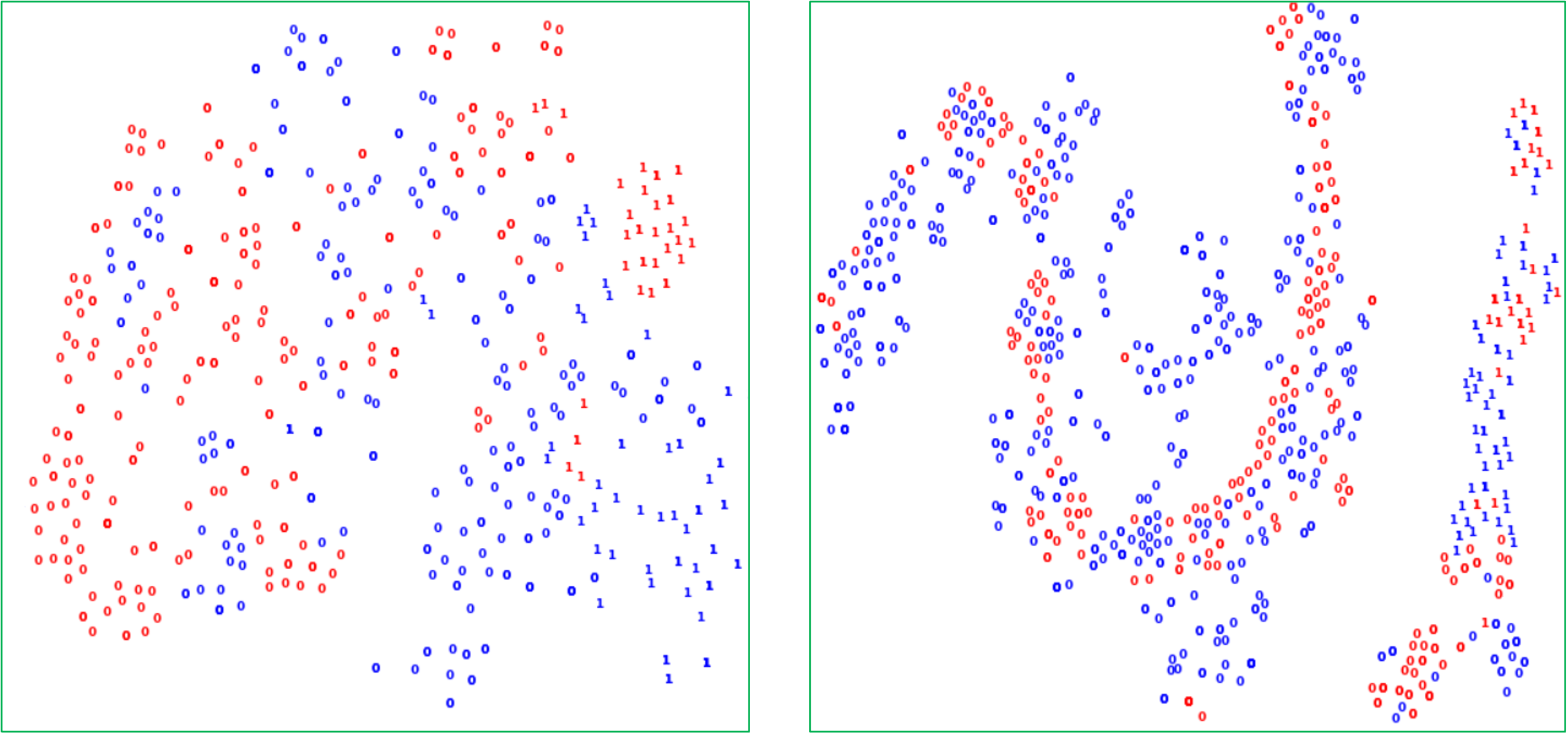
We further demonstrate the efficiency of our proposed method in closing the gap between the source and target domains. We visualize the feature distributions of the source and target domains in the joint space using a 2D t-SNE (Laurens and Geoffrey 2008) projection with perplexity equal to $30$. In particular, we project the source domain and target domain data in the joint space (i.e., $G\left(\boldsymbol{x}\right)$) into a 2D space without undertaking domain adaptation (using the VulDeePecker method) and with undertaking domain adaptation (using our proposed DAM2P method).

In Figure 3, we present the results when performing domain adaptation from a software project (FFmpeg) to another (LibPNG). For the purpose of visualization, we select a random subset of the source project against the entire target project. As shown in Figure 3, without undertaking domain adaptation (VulDeePecker) the blue points (the source domain data) and the red points (the target domain data) are almost separate while with undertaking domain adaptation the blue and red points intermingled as expected. Furthermore, we observe that the mixing-up level of source domain and target domain data using our DAM2P method is significantly higher than using VulDeePecker.

Figure 3: A 2D t-SNE projection for the case of the FFmpeg $\rightarrow$ LibPNG without undertaking domain adaptation (the left-hand figure, using VulDeePecker) and with undertaking domain adaptation (the right-hand figure, using our proposed DAM2P method). The blue and red points represent the source and target domains in the joint space respectively. Data points labeled 0 stand for non-vulnerable samples and data points labeled 1 stand for vulnerable samples. It is noted that our method can not only successfully bridge the gap between the source and target domains but also able to distinguish the non-vulnerable and vulnerable data effectively.

Ablation Study

In this section, we aim to further demonstrate the efficiency of our DAM2P method in transferring the learning of software vulnerabilities from imbalanced labeled source domains to other imbalanced unlabeled target domains as well as the superiority of our novel cross-domain kernel classifier in our DAM2P method for learning and separating vulnerable and non-vulnerable data.

Source $\rightarrow$ Target	Methods	FNR	FPR	Recall	Precision	F1
	VulDeePecker	43.75%	6.72%	56.25%	50%	52.94%
FFmpeg $\rightarrow$	DDAN	35.71%	6.98%	64.29%	60%	62.07%
LibTIFF	Kernel-S	30%	5.56%	70%	58.33%	63.63%
	Kernel-ST	25%	5.68%	75%	64.29%	69.23%
	DAM2P (ours)	14.29%	8.14%	85.71%	63.16%	72.73%
	VulDeePecker	25%	2.17%	75%	75%	75%
FFmpeg $\rightarrow$	DDAN	0%	3.26%	100%	72.73%	84.21%
LibPNG	Kernel-S	0%	4.39%	100%	69.23%	81.81%
	Kernel-ST	0%	3.26%	100%	72.72%	84.21%
	DAM2P (ours)	0%	1.07%	100%	87.50%	93.33%

Table 2: Performance results in terms of false negative rate (FNR), false positive rate (FPR), Recall, Precision and F1-measure (F1) of five cases including (i, VulDeePecker), (ii, DDAN), (iii, Kernel-Source denoted by Kernel-S), (iv, Kernel-Source-Target denoted by Kernel-ST), and (v, DAM2P) for predicting vulnerable and non-vulnerable code functions on the testing set of the target domain (Best performance in bold).

For this ablation study, we conduct experiments on two pairs FFmpeg $\rightarrow$ LibTIFF and FFmpeg $\rightarrow$ LibPNG. We want to demonstrate that bridging the discrepancy gap in the latent space and the max-margin cross-domain kernel classifier are complementary to boost the domain adaptation performance with imbalanced nature. We consider five cases in which we start from the blank case (i, VulDeePecker) without bridging the gap and cross-domain kernel classifier. We then only add the GAN term to bridge the discrepancy gap in the second case (ii, DDAN). In the third case (iii, Kernel-Source), we only apply the max-margin principle for the source domain, while applying the max-margin principle for the source and target domains in the fourth case (iv, Kernel-Source-Target). Finally, in the last case (v, DAM2P), we simultaneously apply the bridging term and the max-margin terms for the source and target domains. The results in Table 2 shows that the max-margin terms and bridging term help to boost the domain adaptation performance. Moreover, applying the max-margin term to both the source and target domains improves the performance comparing to applying to only source domain. Last but not least, bridging the discrepancy gap term in cooperation with the max-margin term significantly improves the domain adaptation performance.

Additional ablation study

Sampling and weighting, and Logit adjustment

Sampling and weighting are well-known as simple and heuristic methods to deal with imbalanced datasets. However, as mentioned by Lin et al. (2017); Cui et al. (2019), these methods may have some limitations, for example, i) Sampling may either introduce large amounts of duplicated samples, which slows down the training and makes the model susceptible to overfitting when oversampling, or discard valuable examples that are important for feature learning when undersampling, and ii) To the highly imbalanced datasets, directly training the model or weighting (e.g., inverse class frequency or the inverse square root of class frequency) cannot yield satisfactory performance.

Menon et al. (2021) recently proposed a novel statistical framework for solving the imbalanced (long-tailed) label distribution problem. Specifically, the framework, revisiting the idea of logit adjustment based on the label frequencies, encourages a large relative margin between logits of the rare positive labels versus the dominant negative labels.

To experience and investigate the efficiency of these methods (i.e., sampling and weighting, and logit adjustment) when applying to the baselines in the context of imbalanced domain adaptation, we conduct an experiment on two pairs of the source and target domains (i.e., FFmpeg $\rightarrow$ LibTIFF and FFmpeg $\rightarrow$ LibPNG) for four main baselines including DDAN, SCDAN, Dual-GD-DDAN, and Dual-GD-SDDAN using (i) the oversampling technique based on SMOTE (Chawla et al. 2002) (i.e., used to create balanced datasets), and (ii) logit adjustment (LA) used in Menon et al. (2021).

The results in Table 3 show that using the oversampling technique cannot help to improve these baseline models’ performance. In particular, the performance of these baselines without using oversampling is always higher than using oversampling on the used datasets in F1-measure (F1), the most important measure used in SVD. This experiment supports our conjecture that in the context of imbalanced domain adaptation when moving target representations to source representations in the latent space to bridge the gap, oversampling the minority class (i.e., vulnerable class) might increase the chance to wrongly mix up vulnerable representations of the target domain and non-vulnerable representations of the source domain, hence leading to a reduction in performance. In our approach, with the support of the max-margin principle, we keep the vulnerable and non-vulnerable representations distant as much as possible when bridging the gap between them in the latent space.

S $\rightarrow$ T	Methods	FNR	FPR	Recall	Precision	F1
	DDAN w/ OS	21%	12.79%	78.57%	50%	61.11%
	DDAN w/ LA	14.29%	15.11%	85.71%	48%	61.53%
	DDAN w/o (OS or LA)	35.71%	6.98%	64.29%	60%	62.07%
	SCDAN w/ OS	25%	5.43%	75%	54.55%	63.16%
	SCDAN w/ LA	11.11%	8.8%	88.89%	50%	64%
FFmpeg $\rightarrow$	SCDAN w/o (OS or LA)	14.29%	5.38%	85.71%	57.14%	68.57%
LibTIFF	Dual-DDAN w/ OS	25%	6.72%	75%	57.14%	64.87%
	Dual-DDAN w/ LA	35.29%	4.50%	64.71%	64.71%	64.71%
	Dual-DDAN w/o (OS or LA)	12.5%	8.2%	87.5%	56%	68.29%
	Dual-SDDAN w/ OS	16.67%	9.1%	83.33%	56%	67%
	Dual-SDDAN w/ LA	43.75%	1.70%	56.25%	90%	69%
	Dual-SDDAN w/o (OS or LA)	35.29%	3.01%	64.71%	73.33%	68.75%
	DDAN w/ OS	28.57%	0%	71.43%	100%	83.33%
	DDAN w/ LA	25%	0%	75%	100%	85.71%
	DDAN w/o (OS or LA)	0%	3.26%	100%	72.73%	84.21%
	SCDAN w/ OS	25%	0%	75%	100%	85.71%
	SCDAN w/ LA	0%	2.17%	100%	80%	88.89%
FFmpeg $\rightarrow$	SCDAN w/o (OS or LA)	12.5%	1.08%	87.5%	87.5%	87.5%
LibPNG	Dual-DDAN w/ OS	14.29%	1.08%	85.71%	85.71%	85.71%
	Dual-DDAN w/ LA	0%	2.15%	100%	77.78%	87.5%
	Dual-DDAN w/o (OS or LA)	0%	2.17%	100%	80%	88.89%
	Dual-SDDAN w/ OS	12.5%	2.17%	87.5%	77.78%	82.35%
	Dual-SDDAN w/ LA	11.11%	1.1%	88.89%	88.89%	88.89%
	Dual-SDDAN w/o (OS or LA)	17.5%	0%	82.5%	100%	90.41%

Table 3: Performance results in terms of false negative rate (FNR), false positive rate (FPR), Recall, Precision, and F1-measure (F1) of DDAN, SCDAN, Dual-GD-DDAN (Dual-DDAN), and Dual-GD-SDDAN (Dual-SDDAN) methods in three cases of with using oversampling (w/ OS), using LA (w/ LA) and without using (oversampling or LA) (w/o (OS or LA)) for predicting vulnerable and non-vulnerable code functions on the testing set of the target domain. We denote Source $\rightarrow$ Target by S $\rightarrow$ T.

Furthermore, the results in Table 3 indicate that using LA can help slightly improve the model’s performance on some cases of the baselines. In particular, LA increases the performance of Dual-SDDAN on FFmpeg $\rightarrow$ LibTIFF as well as DDAN and SCDAN on FFmpeg $\rightarrow$ LibPNG compared to these methods without using LA. However, to DDAN, SCDAN and Dual-DDAN on FFmpeg $\rightarrow$ LibTIFF as well as Dual-DDAN and Dual-SDDAN on FFmpeg $\rightarrow$ LibPNG, LA cannot help improve these models’ performance. In conclusion, using LA can help increase the baseline’s performance in some cases of the used datasets in F1-measure compared to these cases without using LA or using the oversampling technique. However, similar to the oversampling technique, in most cases mentioned in Table 3, LA cannot help improve the baselines’ performance. Furthermore, in the cases where LA helps increase the baseline models’ performance, our proposed method’s performance (mentioned in Table 1) is still significantly higher.

Conclusion

In this paper, in addition to exploiting deep domain adaptation with automatic representation learning for SVD, we have successfully proposed a novel cross-domain kernel classifier leveraging the max-margin principle to significantly improve the capability of the transfer learning of software vulnerabilities from labeled projects into unlabeled ones in order to deal with two crucial issues in SVD including i) learning automatic representations to improve the predictive performance of SVD, and ii) coping with the scarcity of labeled vulnerabilities in projects that require the laborious labeling of code by experts. Our proposed cross-domain kernel classifier can not only effectively deal with the imbalanced datasets but also leverage the information of the unlabeled projects to further improve the classifier’s performance. The experimental results show the superiority of our proposed method compared with other state-of-the-art baselines in terms of the representation learning and transfer learning processes.

Appendix A Appendix

Data Processing and Embedding

We preprocess the source code datasets before inputting them into the deep neural networks (i.e., baselines and our proposed method). Inspired from the baselines, we first standardize the source code by removing comments, blank lines and non-ASCII characters. Secondly, we map user-defined variables to symbolic variable names (e.g., “var1”, “var2”) and user-defined functions to symbolic function names (e.g., “func1”, “func2”). We also replace integer, real and hexadecimal numbers with a generic <number> token and strings with a generic <str> token. We then embed the source code statements into numeric vectors. For example, to the following code statement “if(func2(func3(number,number),&var2) !=var10)”, we tokenize it to a sequence of code tokens (e.g., if,(,func2,(,func3,(,number,number,),&,var2,),!=,var10,)), construct the frequency vector of the statement information, and multiply this frequency vector by a learnable embedding matrix $W^{si}$.

Figure 4: An example of the overall procedure for data processing and embedding. We use a source code function in the C language programming from the FFmpeg project. After the data preprocessing step, we obtain a preprocessed function, and then using the embedding process to obtain the embedded vectors for the code statements of the function.

Figure 4 shows an example of the overall procedure for a source code function processing and embedding. The sequence of $L$ embedding vectors (e.g., $\boldsymbol{x}_{i}=\left[\boldsymbol{x}_{i1},\dots,\boldsymbol{x}_{iL}\right]$), obtained from the data processing and embedding step, of each function (e.g., $\boldsymbol{x}_{i}$ can be from the source domain or the target domain) is then used as the input to deep learning models (e.g., the baselines and our proposed method).

Note that as the baselines, to our proposed method, for handling the sequential properties of the data and to learn the automatic features of the source code functions, we also use a bidirectional recurrent neural network (bidirectional RNN) for both the source and target domains.

Model configuration

For the baselines including VulDeePecker (Li et al. 2018b), and DDAN (Ganin and Lempitsky 2015), MMD (Long et al. 2015), D2GAN (Nguyen et al. 2017), DIRT-T (Shu et al. 2018), HoMM (Chen et al. 2020), LAMDA (Le et al. 2021), SCDAN (Nguyen et al. 2019) using the architecture CDAN proposed in (Nguyen et al. 2019), and Dual-GD-DDAN and Dual-GD-SDDAN (Nguyen et al. 2020), and our proposed DAM2P method, we use one bidirectional recurrent neural network with LSTM (Hochreiter and Schmidhuber 1997) cells where the size of hidden states is in $\{128,256\}$ for the generator $G$ while to the source classifier $C$ used in the baselines and the domain discriminator $D$, we use deep feed-forward neural networks consisting of two hidden layers where the size of each hidden layer is equal to $300$. We embed the statement information in the $150$ dimensional embedding space.

To our proposed method, the trade-off hyper-parameters $\lambda$ and $\alpha$ are in $\{10^{-3},10^{-2},10^{-1}\}$ and $\{10^{-2},10^{-1},10^{0}\}$, respectively, while the hidden size $h$ is in $\{128,256\}$. The dimension of random feature space $2K$ is set equal to $1024$. The length $L$ of each function is padded or cut to 100 or less than 100 code statements (i.e., We base on the quantile values of the functions’ length of each dataset to decide the length of each function). We observe that almost all important information relevant to the vulnerability lies in the 100 first code statements or even lies in some very first code statements.

We employed the Adam optimizer (Kingma and Ba 2014) with an initial learning rate of $10^{-3}$ while the mini-batch size is set to $100$ to our proposed method and baselines. We split the data of the source domain into two random partitions containing 80% for training and 20% for validation. We also split the data of the target domain into two random partitions. The first partition contains 80% for training the models of MMD, D2GAN, DIRT-T, HoMM, LAMDA, DDAN, SCDAN, Dual-GD-DDAN, Dual-GD-SDDAN, and DAM2P without using any label information while the second partition contains 20% for testing the models. We additionally applied gradient clipping regularization to prevent the over-fitting problem in the training process of each model. For each method, we ran the corresponding model $5$ times and reported the averaged measures. We implemented all mentioned methods in Python using Tensorflow (Abadi et al. 2016), an open-source software library for Machine Intelligence developed by the Google Brain Team, on an Intel E5-2680, having 12 CPU Cores at 2.5 GHz with 128GB RAM, integrated NVIDIA Tesla K80.

Figure 5: The correlation between $h$ and F1-measure of our proposed DAM2P method.

Additional experiments

Hyper-parameter Sensitivity

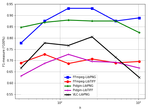
In this section, we investigate the correlation between important hyper-parameters (including the $\lambda$, $\alpha$, and $h$ (the size of hidden states in the bidirectional neural network)) and the F1-measure of our proposed DAM2P method. As mentioned in the experiments section, the trade-off hyper-parameters $\lambda$ and $\alpha$ are in $\{10^{-3},10^{-2},10^{-1}\}$ and $\{10^{-2},10^{-1},10^{0}\}$, respectively, while the hidden size $h$ is in $\{128,256\}$. It is worth noting that we use the commonly used values for the trade-off hyper-parameters ($\lambda$ and $\alpha$) representing for the weights of different terms mentioned in Eq. (6) and the hidden size $h$. In order to study the impact of the hyper-parameters on the performance of the DAM2P method, we use a wider range of values for $\lambda$, $\alpha$, and $h$. In this ablation study, the trade-off parameters $\lambda$ and $\alpha$ are in $\{10^{-4},10^{-3},10^{-2},10^{-1},10^{0},10^{1}\}$ while the hidden size $h$ is in $\{32,64,128,256,512,1024\}$.

Figure 6: The correlation between $\lambda$ and F1-measure of our proposed DAM2P method.

Figure 7: The correlation between $\alpha$ and F1-measure of our proposed DAM2P method.

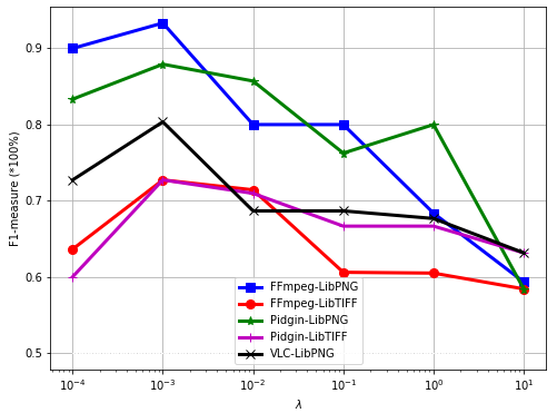
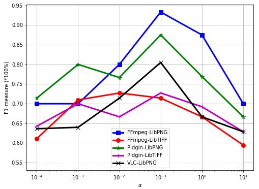
We investigate the impact of $\lambda,\alpha$, and $h$ hyper-parameters on the performance of the DAM2P method on five pairs of the source and target domains including FFmpeg to LibPNG, FFmpeg to LibTIFF, Pidgin to LibPNG, Pidgin to LibTIFF, and VLC to LibPNG. As shown in Figures (5, 6, and 7), we observe that the appropriate values to the hyper-parameters used in the DAM2P model in order to obtain the best model’s performance should be in from $10^{-4}$ to $10^{-2}$, from $10^{-3}$ to $10^{-1}$, and from $64$ to $256$ for $\lambda,\alpha$, and $h$ respectively. In particular, for the hidden size $h$, if we use too small values (e.g., $\leq 32$) or too high values (e.g., $\geq 1024$), the model might encounter the underfitting or overfitting problems respectively. The model’s performance on $\lambda$ (i.e., representing the weight of the information from the target domain contributing to the cross-domain kernel classifier during the training process) shows that we should not set the value of $\lambda$ equal or higher than $1.0$ (i.e., used for the weight of the information from the source domain), and the value of $\lambda$ should be higher than $10^{-4}$ to make sure that we use enough information of the target domain in the training process to improve the cross-domain kernel classifier.

References

- Abadi et al. (2016) Abadi, M.; Barham, P.; Chen, J.; Chen, Z.; Davis, A.; Dean, J.; Devin, M.; Ghemawat, S.; Irving, G.; Isard, M.; et al. 2016. Tensorflow: A system for large-scale machine learning. In 12th USENIX Symposium on Operating Systems Design and Implementation (OSDI 16), 265–283.
- Chawla et al. (2002) Chawla, N. V.; Bowyer, K. W.; Hall, L. O.; and Kegelmeyer, W. P. 2002. SMOTE: synthetic minority over-sampling technique. Journal of Artificial Intelligence Research, 16: 321–357.
- Chen et al. (2020) Chen, C.; Fu, Z.; Chen, Z.; Jin, S.; Cheng, Z.; Jin, X.; and Hua, X. 2020. HoMM: Higher-order Moment Matching for Unsupervised Domain Adaptation. Thirty-Fourth AAAI Conference on Artificial Intelligence.
- Cheng et al. (2019) Cheng, X.; Wang, H.; Hua, J.; Zhang, M.; Xu, G.; Yi, L.; and Sui, Y. 2019. Static Detection of Control-Flow-Related Vulnerabilities Using Graph Embedding. In 2019 24th International Conference on Engineering of Complex Computer Systems (ICECCS).
- Cui et al. (2019) Cui, Y.; Jia, M.; Lin, T.; Song, Y.; and Belongie, S. J. 2019. Class-Balanced Loss Based on Effective Number of Samples. CoRR, abs/1901.05555.
- Dam et al. (2018) Dam, H. K.; Tran, T.; Pham, T.; Wee, N. S.; Grundy, J.; and Ghose, A. 2018. Automatic feature learning for predicting vulnerable software components. IEEE Transactions on Software Engineering.
- Dowd, McDonald, and Schuh (2006) Dowd, M.; McDonald, J.; and Schuh, J. 2006. The Art of Software Security Assessment: Identifying and Preventing Software Vulnerabilities. Addison-Wesley Professional. ISBN 0321444426.
- Duan et al. (2019) Duan, X.; Wu, J.; Ji, S.; Rui, Z.; Luo, T.; Yang, M.; and Wu, Y. 2019. VulSniper: Focus Your Attention to Shoot Fine-Grained Vulnerabilities. In Proceedings of the Twenty-Eighth International Joint Conference on Artificial Intelligence, IJCAI-19.
- Ganin and Lempitsky (2015) Ganin, Y.; and Lempitsky, V. 2015. Unsupervised Domain Adaptation by Backpropagation. In Proceedings of the 32nd International Conference on International Conference on Machine Learning - Volume 37, ICML’15, 1180–1189.
- Goodfellow et al. (2014) Goodfellow, I.; Pouget-Abadie, J.; Mirza, M.; Xu, B.; Warde-Farley, D.; Ozair, S.; Courville, A.; and Bengio, Y. 2014. Generative adversarial nets. In Advances in neural information processing systems, 2672–2680.
- Grieco et al. (2016) Grieco, G.; Grinblat, G. L.; Uzal, L.; Rawat, S.; Feist, J.; and Mounier, L. 2016. Toward Large-Scale Vulnerability Discovery Using Machine Learning. In Proceedings of the Sixth ACM Conference on Data and Application Security and Privacy, CODASPY ’16, 85–96. ISBN 978-1-4503-3935-3.
- Hochreiter and Schmidhuber (1997) Hochreiter, S.; and Schmidhuber, J. 1997. Long Short-Term Memory. Neural Computation, 9(8): 1735–1780.
- Kim et al. (2017) Kim, S.; Woo, S.; Lee, H.; and Oh, H. 2017. VUDDY: A Scalable Approach for Vulnerable Code Clone Discovery. In IEEE Symposium on Security and Privacy, 595–614. IEEE Computer Society.
- Kingma and Ba (2014) Kingma, D. P.; and Ba, J. 2014. Adam: A Method for Stochastic Optimization. CoRR, abs/1412.6980.
- Kipf and Welling (2016) Kipf, T. N.; and Welling, M. 2016. Semi-Supervised Classification with Graph Convolutional Networks. CoRR, abs/1609.02907.
- Laurens and Geoffrey (2008) Laurens, V. M.; and Geoffrey, H. 2008. Visualizing Data using t-SNE. Journal of Machine Learning Research.
- Le et al. (2021) Le, T.; Nguyen, T.; Ho, N.; Bui, H.; and Phung, D. 2021. LAMDA: Label Matching Deep Domain Adaptation. In Proceedings of the 38th International Conference on Machine Learning, 6043–6054.
- Le et al. (2010) Le, T.; Tran, D.; Ma, W.; and Sharma, D. 2010. An optimal sphere and two large margins approach for novelty detection. In Neural Networks (IJCNN), The 2010 International Joint Conference on, 1–6.
- Li et al. (2016) Li, Z.; Zou, D.; Xu, S.; Jin, H.; Qi, H.; and Hu, J. 2016. VulPecker: An Automated Vulnerability Detection System Based on Code Similarity Analysis. In Proceedings of the 32Nd Annual Conference on Computer Security Applications, ACSAC ’16, 201–213. ISBN 978-1-4503-4771-6.
- Li et al. (2018a) Li, Z.; Zou, D.; Xu, S.; Jin, H.; Zhu, Y.; Chen, Z.; Wang, S.; and Wang, J. 2018a. SySeVR: A Framework for Using Deep Learning to Detect Software Vulnerabilities. CoRR, abs/1807.06756.
- Li et al. (2018b) Li, Z.; Zou, D.; Xu, S.; Ou, X.; Jin, H.; Wang, S.; Deng, Z.; and Zhong, Y. 2018b. VulDeePecker: A Deep Learning-Based System for Vulnerability Detection. CoRR, abs/1801.01681.
- Lin et al. (2018) Lin, G.; Zhang, J.; Luo, W.; Pan, L.; Xiang, Y.; Olivier, D. V.; and Paul, M. 2018. Cross-Project Transfer Representation Learning for Vulnerable Function Discovery. In IEEE Transactions on Industrial Informatics, volume 14.
- Lin et al. (2017) Lin, T.; Goyal, P.; Girshick, R. B.; He, K.; and Dollár, P. 2017. Focal Loss for Dense Object Detection. CoRR, abs/1708.02002.
- Liu et al. (2020) Liu, S.; Lin, G.; Qu, L.; Zhang, J.; De Vel, O.; Montague, P.; and Xiang, Y. 2020. CD-VulD: Cross-Domain Vulnerability Discovery based on Deep Domain Adaptation. IEEE Transactions on Dependable and Secure Computing.
- Long et al. (2015) Long, M.; Cao, Y.; Wang, J.; and Jordan, M. 2015. Learning Transferable Features with Deep Adaptation Networks. In Proceedings of the 32nd International Conference on Machine Learning, 97–105.
- Menon et al. (2021) Menon, A. K.; Jayasumana, S.; Rawat, A. S.; Jain, H.; Veit, A.; and Kumar, S. 2021. Long-tail learning via logit adjustment. International Conference on Learning Representations.
- Neuhaus et al. (2007) Neuhaus, S.; Zimmermann, T.; Holler, C.; and Zeller, A. 2007. Predicting Vulnerable Software Components. In Proceedings of the 14th ACM Conference on Computer and Communications Security, CCS ’07, 529–540. ISBN 978-1-59593-703-2.
- Nguyen et al. (2017) Nguyen, T. D.; Le, T.; Vu, H.; and Phung, D. Q. 2017. Dual Discriminator Generative Adversarial Nets. CoRR, abs/1709.03831.
- Nguyen et al. (2020) Nguyen, V.; Le, T.; De Vel, O.; Montague, P.; Grundy, J.; and Phung, D. 2020. Dual-Component Deep Domain Adaptation: A New Approach for Cross Project Software Vulnerability Detection.
- Nguyen et al. (2019) Nguyen, V.; Le, T.; Le, T.; Nguyen, K.; DeVel, O.; Montague, P.; Qu, L.; and Phung, D. 2019. Deep Domain Adaptation for Vulnerable Code Function Identification. In The International Joint Conference on Neural Networks (IJCNN).
- Nguyen et al. (2014) Nguyen, V.; Le, T.; Pham, T.; Dinh, M.; and Le, T. H. 2014. Kernel-based semi-supervised learning for novelty detection. In 2014 International Joint Conference on Neural Networks (IJCNN), 4129–4136.
- Rahimi and Recht (2008) Rahimi, A.; and Recht, B. 2008. Random Features for Large-Scale Kernel Machines. In Advances in Neural Information Processing Systems.
- Russell et al. (2018) Russell, R. L.; Kim, L. Y.; Hamilton, L. H.; Lazovich, T.; Harer, J. A.; Ozdemir, O.; Ellingwood, P. M.; and McConley, M. W. 2018. Automated Vulnerability Detection in Source Code Using Deep Representation Learning. CoRR, abs/1807.04320.
- Schölkopf et al. (2001) Schölkopf, B.; Platt, J. C.; Shawe-Taylor, J. C.; Smola, A. J.; and Williamson, R. C. 2001. Estimating the Support of a High-Dimensional Distribution. Neural Comput., 13(7): 1443–1471.
- Shin et al. (2011) Shin, Y.; Meneely, A.; Williams, L.; and Osborne, J. A. 2011. Evaluating complexity, code churn, and developer activity metrics as indicators of software vulnerabilities. IEEE Transactions on Software Engineering, 37(6): 772–787.
- Shu et al. (2018) Shu, R.; Bui, H.; Narui, H.; and Ermon, S. 2018. A DIRT-T Approach to Unsupervised Domain Adaptation. In International Conference on Learning Representations.
- Tax and Duin (2004) Tax, D. M. J.; and Duin, R. P. W. 2004. Support Vector Data Description. Journal of Machine Learning Research, 54(1): 45–66.
- Tsang, Kocsor, and Kwok (2007) Tsang, I. W.; Kocsor, A.; and Kwok, J. T. 2007. Simpler Core Vector Machines with Enclosing Balls. In Proceedings of the 24th International Conference on Machine Learning, ICML ’07, 911–918.
- Tsang et al. (2005) Tsang, I. W.; Kwok, J. T.; Cheung, P.; and Cristianini, N. 2005. Core vector machines: Fast SVM training on very large data sets. Journal of Machine Learning Research, 6: 363–392.
- Yamaguchi, Lindner, and Rieck (2011) Yamaguchi, F.; Lindner, F.; and Rieck, K. 2011. Vulnerability extrapolation: assisted discovery of vulnerabilities using machine learning. In Proceedings of the 5th USENIX conference on Offensive technologies, 13–23.
- Zhuang et al. (2020) Zhuang, Y.; Liu, Z.; Qian, P.; Liu, Q.; Wang, X.; and He, Q. 2020. Smart Contract Vulnerability Detection using Graph Neural Network. In Proceedings of the Twenty-Ninth International Joint Conference on Artificial Intelligence, IJCAI-20.
- Zimmermann et al. (2009) Zimmermann, T.; Nagappan, N.; Gall, H.; Giger, E.; and Murphy, B. 2009. Cross-project Defect Prediction: A Large Scale Experiment on Data vs. Domain vs. Process. In Proceedings of the the 7th Joint Meeting of the European Software Engineering Conference and the ACM SIGSOFT Symposium on The Foundations of Software Engineering, ESEC/FSE ’09, 91–100. ISBN 978-1-60558-001-2.