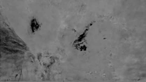
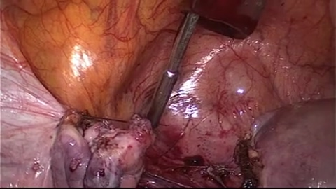
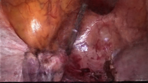
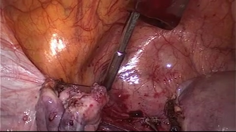
wildNeRF: Complete view synthesis of in-the-wild dynamic scenes captured using sparse monocular data

Abstract

We present a novel neural radiance model that is trainable in a self-supervised manner for novel-view synthesis of dynamic unstructured scenes. Our end-to-end trainable algorithm learns highly complex, real-world static scenes within seconds and dynamic scenes with both rigid and non-rigid motion within minutes. By differentiating between static and motion-centric pixels, we create high-quality representations from a sparse set of images. We perform extensive qualitative and quantitative evaluation on existing benchmarks and set the state-of-the-art on performance measures on the challenging NVIDIA Dynamic Scenes Dataset. Additionally, we evaluate our model performance on challenging real-world datasets such as Cholec80 and SurgicalActions160.

1 Introduction

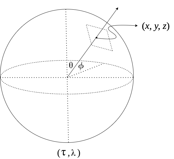
Visual scene understanding is a long-standing problem in computer vision. The ability of machine learning models to identify, cluster, classify, and track pixels within and across frames has seen tremendous growth over the last decade. Recently, novel-view synthesis and novel-time synthesis have gained significant traction because of neural radiance-based methods [31, 34, 29, 1, 35] that combine deep learning approaches and classical vision modelling. This allows for fine-grained reconstructions in 3D space. These models take a sparse set of input frames as input, from which camera pose information is extracted [41]. A complete scene is generated by modelling a 7D scene representation $f(x,y,z,\theta,\phi,\lambda,\tau)$ where $x,y,z$ are spatial locations and $\theta,\phi$ are camera pose parameters. This generalized representation is known as the Plenoptic function as it describes all image information visible from a particular viewing position [4], for different wavelengths $\lambda$ and time $\tau$. This function may be constrained to a 6D representation by assuming a constant wavelength, $\lambda$. This representation has various real-world applications, including depth estimation [7, 13], 3D tracking [59, 22], and video stabilization [26, 55]. We illustrate this generalized formulation in Figure 2.

Despite significant advances, existing model architectures are still limited. $1.$ They are extremely computationally intensive and can take days to create believable representations of very small scenes [29, 34, 35]. Various works [33, 38, 57, 10] leverage inefficiencies in neural-radiance architectures and incorporate massively parallel algorithms to speed-up reconstruction times. $2.$ The problem is extremely under constrained; e.g., learning a 6D representation from, in some cases, a set of 12 sparse inputs (NVIDIA dynamic scenes dataset [56]) leads to significant artifacts along the time axis. $3.$ Traditional NeRF-based [29] reconstructions use sparse inputs captured in a more holistic manner to allow for easier generalization.

Figure 2: A generalized representation of the Plenoptic function. We constrain the function by considering only pixel coordinates $(x,y,z)$, camera parameters $(\theta,\phi)$, and time $(\tau)$, and assuming a constant wavelength $(\lambda)$.

Our contributions are as follows: $1.$ We showcase the efficacy of our model using the publicly available NVIDIA dynamic scenes dataset and extend our model to real-world datasets such as the SurgicalActions160 [40] and Cholec80 [47] datasets. $2.$ To the best of our knowledge, this is the first paper to incorporate CUDA-accelerated training schemes for monocular dynamic scenes, thereby increasing the applicability of such models to applications. $3.$ We extend state-of-the-art techniques by Li et al [23] and Gao et al [11] to successfully model both rigid and non-rigid motion. $4.$ We apply this approach to extremely challenging surgical datasets for the purpose of 3D instrument-tracking and video stabilization, the successful implementation of which would open the door to exciting new advances in surgical skill evaluation [18, 19].

2 Related Work

To truly understand scenes, 2D representations are insufficient and thus significant strides have been made in recent years to create highly representative 3D representations. That work is mostly centered around static or rigid geometries such as point-clouds [15, 3, 51, 44], voxels [43, 60, 52, 20], octrees [50, 57], or various computed tomography algorithms [6]. However, these representations are computationally intensive and are seldom extendable to dynamic and non-rigid scenes. Recent advances in implicit functions for representing scenes have shown the ability to implicitly encode photometric attributes such as colour, surface illumination, opacity etc. using shallow neural nets [29, 1, 35, 30], an important characteristic of these approaches is that they are usually self-supervised. The models can be trained in an end-to-end manner by leveraging a pixel-wise photometric reconstruction loss, which is in strong contrast to existing approaches that require strong priors [9, 39, 17] or existing templates [34, 14, 54, 53, 49], each of which are challenging to acquire and significantly limit the generalizability of these approaches to ideal pre-designed scenes.

Some approaches within the implicit representation paradigm have shown the ability to generate incredibly detailed scenes from a limited set of images [35, 34, 23, 11]. These immaculate reconstructions illustrate an important proof-of-concept and the expressibility of well-crafted representations, but aren’t directly extendable to in-the-wild scenes. This is because the input images, although sparse, are well-posed, capture a $360\deg$ panoramic view of the scene, and must come with pre-computed pose information. In-the-wild scenes are generally captured from a monocular source and do not include pose information. This information is calculated using off-the-shelf models that use structure-from-motion for calculating camera pose and are non-deterministic, and thus prone to error [41].

Some approaches extend the implicit representation paradigm to include time $\tau$. These are highly relevant to this paper; specifically, in-the-wild approaches that are extremely under-constrained and require off-the-shelf models. Flow-based methods such as [23, 11] use off-the-shelf methods to constrain the scene by using additional inputs such as depth estimation [21], optical flow [2, 45], and semantic segmentation [12]. Additionally, some work has been done using deformation-based approaches [36, 46] to model dynamic scenes. Although that work is agnostic to input data, and depend on neither pre-trained models nor pre-designed priors, it doesn’t generalize well to in-the-wild scenes. Our approach combines existing flow-based approaches with deformation-based approaches to set the state-of-the-art on the NVIDIA dynamic scenes dataset.

We also leverage the work done in multi-resolution encoding, which have shown the ability to significantly improve reconstructions by encoding data as a multi-resolution subset of high-frequency embeddings, as measured by commonly-used reconstruction metrics, Learned Perceptual Image Patch Similarity (LPIPS) [58], Structural Similarity (SSIM) [5], and peak Signal-to-noise ratio (PSNR) [16].

Figure 3: Our proposed end-to-end trainable architecture. We use density and colour networks (top) to model a static representation of the scene, and density, colour, and deformation networks (bottom) to model the motion-centric pixels in the image. Each set of representations are trained separately and the final image consists of the fused output, as described in section 3.5.4.

3 Method

We introduce wildNeRF, a computationally-efficient neural renderer for novel view and time synthesis tasks. The proposed renderer reconstructs complex scenes from sparse inputs captured using a monocular camera source. We build on prior work on flow-based [23, 11] and deformation-based [36, 46] approaches to model dynamic scenes using computationally efficient grid embeddings [33]. These approaches extend traditional neural radiance representations by modelling the change in geometry of objects in the scene over time. This yields high-fidelity reconstructions of complex scenes with varying geometries and intricate dynamics. We illustrate that a combination of deformation and flow-based techniques is able to capture scenes in a holistic manner without loss of generality on novel-view and novel-time synthesis tasks. We leverage off-the-shelf pre-trained models for generating flow [45] and depth priors [21] to constrain the canonical reconstruction space, leading to high-quality reconstructions. We also leverage effective grid encodings [33] to produce results in a fraction of the time of existing models.

3.1 Datasets

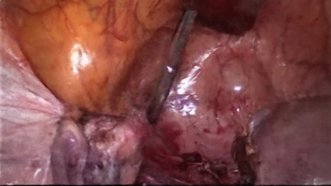
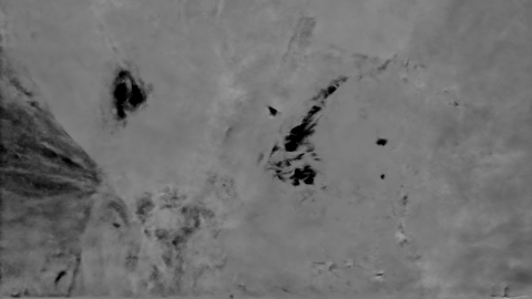
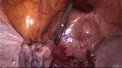
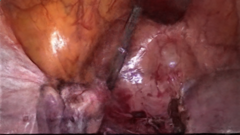
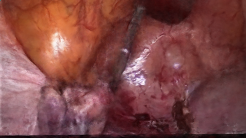
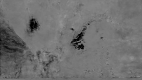
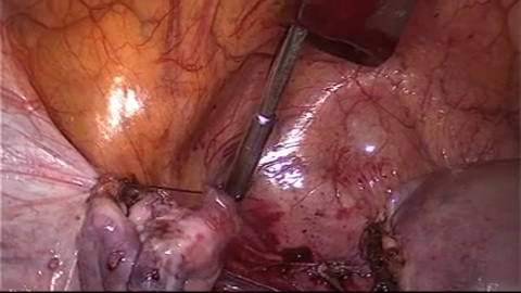
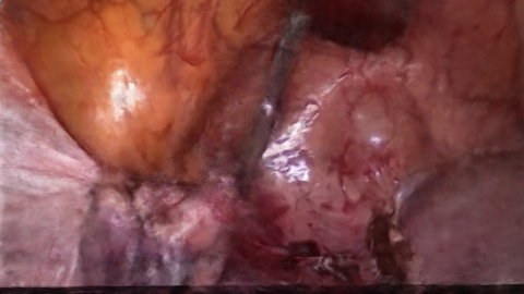
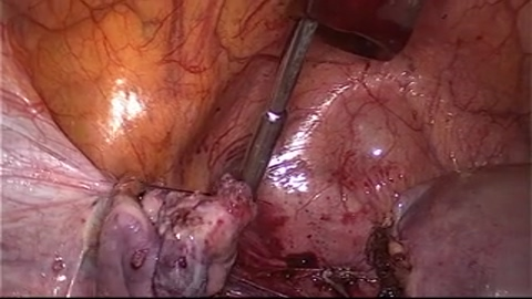
In this paper, we show quantitative and qualitative results on the NVIDIA Dynamic Scenes Dataset [56], and qualitative results (due to the lack of ground truth depth data) on complex surgical datasets, Cholec80 [47] and SugicalActions160 [40], which deal with significant unstructured motion between the camera and the objects in a scene.

NVIDIA Dynamic Scenes Dataset: This dataset consists of 8 scenes, each captured using 12 synchronized cameras to mimic motion. In each case, 24 frames from the dataset are held out and used for training and 12 are set aside for testing.

Cholec80: This dataset contains 80 full-length surgical videos capturing the cholecystectomy procedure. The scope of existing neural radiance field approaches are limited since they can only model very constrained scenes consisting of a small set of frames. We thus focus on short clips extracted from the longer videos to evaluate the efficacy of these approaches in extremely unconstrained environments.

SurgicalActions160: This dataset consists of a total of 160 short clips ($\sim$5 seconds) in which surgeons perform critical actions such as suturing, dissection, and knotting.

3.2 Scene registration

To completely learn a scene, we require relative camera pose information as input along with image coordinates. Extracting this information from a set of sparse images is called ‘scene registration’, where the structure of features within a scene are used to generate the relative pose characteristics of the constituent images, this is a well studied problem in computer vision and visual perception, called structure-from-motion. We use COLMAP [41], an open-source structure-from-motion library, for this purpose.

3.3 Volume rendering

We build on the original NeRF [31] formulation and describe the volume rendering equations used in our analysis. We parameterize a ray extending from its point of origin o, with direction d as follows: $y(\textit{b})=\textbf{o}+\textit{b}.\textbf{d}$. Where b refers to a uniformly sampled point along the ray that exists within the near and far bounds, $b_{n}$ and $b_{f}$ respectively. Using this formulation, we can define a generalized version of the the expected colour C of a pixel as follows:

$$C(\Theta)=\int_{b_{n}}^{b_{f}}{\color[rgb]{1,0,0}\underbrace{\tau(b,\Theta)}_{\textrm{Transmissivity}}}{\color[rgb]{0,0,1}\underbrace{\sigma(\textbf{p}(b,\Theta))}_{\textrm{Pixel density}}}{\color[rgb]{.75,.5,.25}\underbrace{c(\textbf{p}(b,\Theta),d)}_{\textrm{Pixel colour}}}db$$ (1)

The transmittance $\tau$ defined in eq.1 is the probability that a ray between points $b_{n}$ and $b$ is absorbed, scattered, or reflected by other objects in its path.

$${\color[rgb]{1,0,0}\tau(b,\Theta)}=e^{\int_{b_{n}}^{b}\sigma(p(b,\Theta))db}$$ (2)

$${\color[rgb]{0,0,1}\sigma(\textbf{p}(b,\Theta))}=f_{\phi}(\textbf{p}(b,\Theta))$$ (3)

$${\color[rgb]{.75,.5,.25}c(\textbf{p}(b,\Theta),\textbf{d})}=f_{\theta}(\textbf{p}(b,\Theta),\textbf{d})$$ (4)

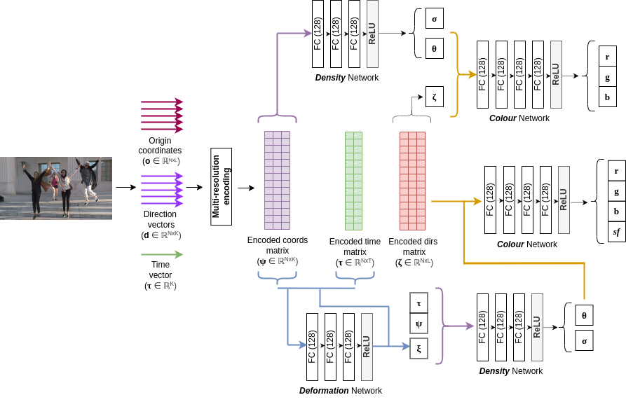
Equations 3 and 4 are outputs of fully-connected models, details of which are depicted in Figure 3. $\Theta$ is the set of variables that parameterize the model. When modelling rigid or non-rigid body motion, $\Theta=(x,d,t)$ where $x$, $d$ and $t$ refer to the input points, input directions, and input time, respectively. As in previous work [31], we use numerical quadrature [27] to approximate these integrals. We uniformly sample a set of evenly-spaced points between the near and far bounds, $b_{n}$ and $b_{f}$. The resulting equations are as follows:

$$C(\Theta)=\sum_{b=1}^{N}{\color[rgb]{1,0,0}\underbrace{\tau(b,\Theta)}_{\textrm{Transmissivity}}}{\color[rgb]{0,0,1}\underbrace{\alpha(\textbf{p}(b,\Theta,\delta))}_{\textrm{Pixel density}}}{\color[rgb]{.75,.5,.25}\underbrace{c(\textbf{p}(b,\Theta),d)}_{\textrm{Pixel colour}}}$$ (5)

$${\color[rgb]{1,0,0}\tau(b,\Theta)}=e^{-\sum_{b_{n}}^{b}\sigma(\textbf{p}(b,\Theta))\delta_{n}}$$ (6)

$${\color[rgb]{0,0,1}\alpha(b,\Theta,\delta)}=1-e^{-\sigma(\textbf{p}(b,\Theta))\delta_{n}},$$ (7)

where $\sigma$ and c are model outputs (Figure 3), and $\delta_{n}=b_{n+1}-b_{n}$ is the distance between two consecutive quadrature points.

3.4 Pixel pruning

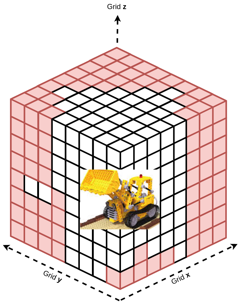
Traditional approaches [29, 31, 30] have used strategically designed coarse and fine sampling schedules of subtended rays for calculating colour pixel values, eq. 5. Our approach is inspired by recent advances in efficient training methods of voxel based models [42, 25, 28] in which we systematically turn-off points in space that don’t contribute to our scene for a fixed number of iterations. In doing so, we significantly reduce the number of matrix operations required in downstream calculations. After $N=5000$ iterations, we continue optimizing the most representative pixels in the image. We illustrate our approach in Figure 4

Figure 4: Illustration of the pixel pruning process. Over the first few iterations of the model, any pixel on our grid illustrated as red is excluded from the analysis.

Figure 5: Predicted flow across frames generated by the scene-flow model. These predictions, in conjunction with off-the-shelf estimations of rigid-body flow, help constrain our extremely under-constrained scene.

3.5 Model architecture

Our proposed renderer consists of 3 core lightweight fully-connected models, a flow model for predicting the scene-flow, a deformation model for modelling non rigid-body dynamics of the model from one frame, to the next, and a background model that is agnostic of any motion-centric pixels in the scene. We illustrate the two predictive outputs and how they are used for training the model in an end-to-end manner in Figure 3.

3.5.1 Background Network

We model the pixels associated with rigid bodies in a scene using a conventional radiance-based implicit representation model [31]. We mask the motion-centric pixels and use numeric quadrature approximations (Eq. 5) to map the canonical scene coordinates to the corresponding 2D pixels. For a fair comparison against results in literature, we use $N=256$ uniformly sampled points along each ray. The static paradigm can thus be represented as follows:

$$\sigma^{static}=f_{\theta}(r(p_{n}))$$ (8)

$$c^{static}=f_{\phi}(r(p_{n}),d),$$ (9)

where the functions $f_{\theta}$ and $f_{\phi}$ are represented using the static fully connected models illustrated in Figure 3.

$$C^{s}(x,d)=\sum_{b=1}^{N}\underbrace{\tau(b,x,d)}_{\textrm{Transmissivity}}\underbrace{\alpha(p(b,x,d,\delta))}_{\textrm{Pixel density}}\underbrace{c(p(b,x,d),d)}_{\textrm{Pixel colour}}$$ (10)

$${\color[rgb]{1,0,0}\mathcal{L}^{s}}=\sum_{n}||C^{s}-C^{gt}||_{2}^{2}$$ (11)

where $M$ is pre-calculated pixel mask that denotes the presence of motion-centric pixels in the training data.

3.5.2 Deformation network

We model non-rigid motion across frames by defining a transformation $\Delta x$, that is applied to points in canonical space across different instances in time. This deformation, $\phi$, jointly with flow-based rigid body motion modelling allows us to improve on existing state-of-the-art results on the NVIDIA dynamic scenes dataset. This transformation is learned by minimizing the mean squared error over the entire dataset.

$$\Delta x=f_{\psi}(x,d,t)$$ (12)

$$x^{*}=x+\Delta x,$$ (13)

where $x^{*}$ is our predicted non-rigid body deformation, which is included in our downstream analysis.

3.5.3 Scene-flow network

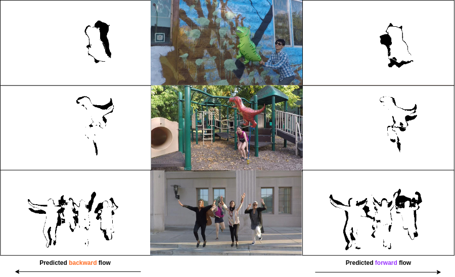
As is the case when attempting to model a large set, of variables using the plenoptic function, the scene becomes increasingly under-constrained. We address these anomalies by leveraging photometric constraints to model rigid-body motion of dynamic pixels in our scene. We model the flow field of the non-rigid motion across adjacent frames in both the forward ($t_{c}=t+1$) and backward ($t_{c}=t-1$) directions (Figure 5). The flow field is determined as follows:

$$(sf_{b},sf_{f},\sigma_{t}^{dynamic},c_{t}^{dynamic})=f_{\phi}(x^{*},d,t)$$ (14)

$$(sf_{t-1}^{b},sf_{t-1}^{f},\sigma_{t-1}^{dynamic},c_{t-1}^{dynamic})=f_{\phi}(x^{*},d,t-1)$$ (15)

$$(sf_{t+1}^{b},sf_{t+1}^{f},\sigma_{t+1}^{dynamic},c_{t+1}^{dynamic})=f_{\phi}(x^{*},d,t+1),$$ (16)

where $x^{*}$, $d$, and $t$ refer to the pixels in canonical space, their direction vectors, and instances in time.

We extend eq. 10 to the case of rigid-body motion as follows:

$$C^{d}(\Theta,t)=\sum_{b=1}^{N}\underbrace{\tau(b,\Theta,t)}_{\textrm{Transmissivity}}\underbrace{\alpha(p(b,\Theta,t,\delta))}_{\textrm{Pixel density}}\underbrace{c(p(b,\Theta,t),d)}_{\textrm{Pixel colour}}$$ (17)

$$where,\Theta=(x^{*},d)$$

The subsequent fields predicted by the model are compared against the corresponding ground truth images ($C^{gt}$). The overall scene-flow photometric loss is represented as:

$${\color[rgb]{0,0,1}\mathcal{L}^{sf+\psi}}=\sum_{n=1}^{N}(||C_{t}^{d}-C_{t}^{gt}||_{2}^{2}+||C_{t-1}^{d}-C_{t-1}^{gt}||_{2}^{2}+$$ (18)

$$||C_{t+1}^{d}-C_{t+1}^{gt}||_{2}^{2})$$

The scene flow loss is carefully designed to constrain rigid motion across frames eq. 19. We illustrate the predicted scene-flow in Figure 5.

Figure 6: Errors encountered during novel-view synthesis reconstruction.

(a) NeRF

(b) NeRF+time

(c) Yoon et al.

(d) Tretschk et al.

(e) Li et al.

(f) Gao et al.

(g) Ours

(h) Ground Truth

Figure 7: Qualitative results: We compare our qualitative results to existing approaches and notice that our results are competitive with existing state-of-the-art approaches such as NSFF and Dynamic NeRF despite only being trained for a fraction of the time. We compare and contrast the training speeds in Table 1

Method	Train Time (hours) $\downarrow$	Speedup $\uparrow$
NeRF [31] (naive)	48 (0.1)	x32
Tretschk et al. [46]	15 (0.1)	5x
Li et al. [23]	50 (0.3)	x35
Gao et al. [11]	48 (0.3)	x33
Ours (w/o pruning)	1.7 (0.1)	x1.1
Ours	1.6 (0.1)	-

Table 1: All experiments were done using an RTX3090 GPU. We present the processing times required to produce the reported PSNR values in Table 2. The speedup column indicates the speedup of the proposed method compared to our method, both with and without pixel pruning 3.4.

3.5.4 Blending approach

Our blending approach utilizes the readily available motion masks generated during the pre-processing step and assigns pixel-level values depending on the masks value. This blending approach is simple and doesn’t require additional networks [36] to model the background pixels. It also avoids a blending parameter that is computed in addition to other network outputs as in [23, 11], each of which require significantly higher computational times and trainable parameters. The final image is computed as follows:

$$C(p)=\begin{cases}C(p)^{dynamic},&\text{if }M\geq 0.5\\ C(p)^{static},&\text{otherwise}\end{cases}$$

3.6 Training Details

For training, we use the pixel-level motion masks to delineate between the static and motion-centric pixels (caused by both rigid and non-rigid motion) in the image. Each image was resized to $480\times 270$ to remain consistent with previous approaches. We sample a set of $N=4096$ rays subtending from these pixels and use them to train to separate models, a simple static or background model, inspired by the original NeRF [31] formulation, and a dynamic or motion-centric model, consisting of an in-built deformation network. This schema allowed us to run all our experiments on an RTX3090 GPU with 24Gb of VRAM. We use an ADAM optimized training scheme, with $l_{r}^{network}=1e-3$ and $l_{r}^{model}=1e-2$. We also use a learning rate scheduler and an exponential decay value of $5e-5$. Finally, our overall loss is calculated as follows:

$$\mathcal{L}^{total}={\color[rgb]{1,0,0}\mathcal{L}^{s}}+{\color[rgb]{0,0,1}\mathcal{L}^{sf+\psi}}$$ (19)

4 Results

4.1 Experimental setup

We evaluate our proposed algorithm on the Dynamic Scene Dataset [56]. The dataset consists of 9 video sequences each captured simultaneously using 12 fixed cameras at 12 time steps. The input for each model is a set of frames ${I_{ct}}$, where c refers to the camera pose and t refers to an instance in time. Figure 3 illustrates the problem setup as we take individual frames at different points in time and attempt to create a generalizable model for predicting novel-view and novel-time states, should one of the controllable parameters $(c,t)$ be fixed. We use COLMAP [41], a commonly used structure-to-motion model that leverages structural information captured from disjointed frames to create a relative mapping in an unsupervised manner, thus yielding pose information for our input frames. Our setup also uses motion-masking to differentiate between static and motion-centric pixels similar to Gao et al [11]. We discuss our quantitative and qualitative results in the sections below.

4.2 Quantitative

We present our quantitative results against state-of-the-art benchmarks in Table 2. We observe improvements of $~{}3\%$ and $~{}1\%$ in Peak signal-to-noise ratio (PSNR - $\uparrow$) and Structural Similarity (SSIM - $\uparrow$) respectively, despite only training for a fraction of the time as earlier works [23, 11, 31]. Additionally, we present a comparison of the training times required by existing approaches in Table 1 and show that pixel pruning (Section 3.4) and a grid generated using a combination of frequency encoding [31] and multi-resolution hash encoding [33] generates results in unparalleled times on complex dynamic scenes. We also observe that most scenes samples are competitive against existing approaches except the Truck scene. We believe that this is due to inconsistent camera pose parameters generated by COLMAP. Dissimilar to other scenes, both the Truck and DynamicFaces scenes required multiple runs of COLMAP as it would regularly fail, as has been documented in earlier works [23, 11]. This inconsistent behaviour is an unfortunate by-product of the structure-from-motion paradigm and is an active area of research [24, 29, 48].

4.3 Qualitative

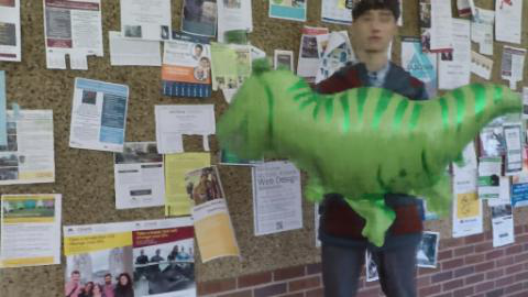
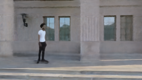
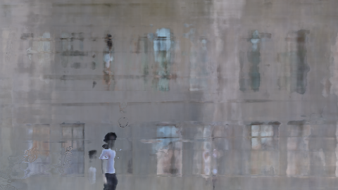
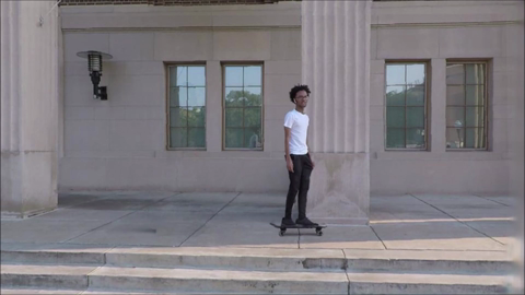
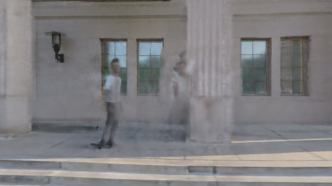
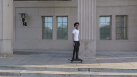
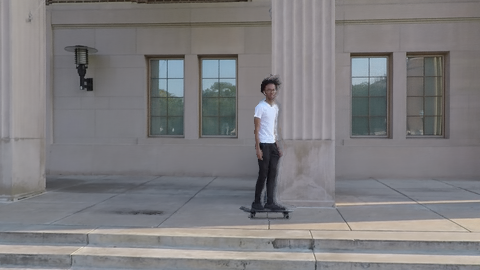
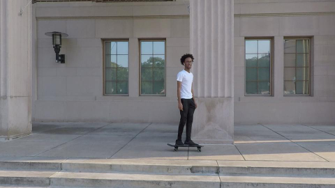
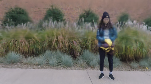
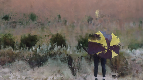
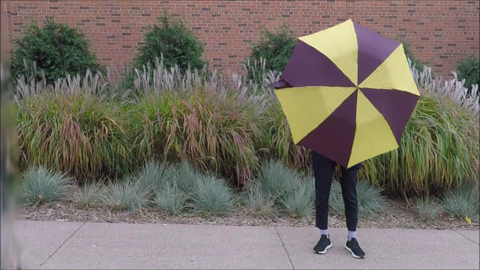
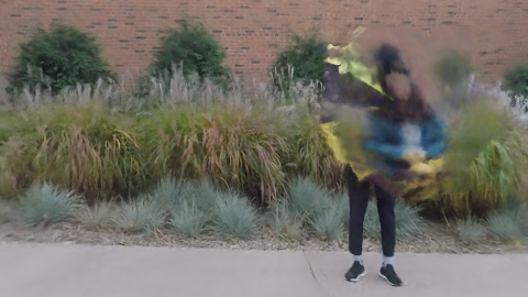
We present our qualitative results against state-of-the-art benchmarks in Figure 7. Our results are highly competitive against earlier approaches and avoid significant artifacts due to motion, such as the entire object disappearing, or even complete reconstruction failure. Gao et al. [11] have shown some of the most impressive results on this dataset, yet they note in the paper that their approach leads to artifacts when modelling non-rigid motion. This can be seen in (Figure 7 - column $(f)$). Our approach is not only able to model both rigid and non-rigid motion but is also able to capture light-based effects well (Figure 7 - column $(g)$).

	Jumping			Skating			Truck			Umbrella
	PSNR $(\uparrow)$	SSIM $(\uparrow)$	LPIPS $(\downarrow)$	PSNR $(\uparrow)$	SSIM $(\uparrow)$	LPIPS $(\downarrow)$	PSNR $(\uparrow)$	SSIM $(\uparrow)$	LPIPS $(\downarrow)$	PSNR $(\uparrow)$	SSIM $(\uparrow)$	LPIPS $(\downarrow)$
NeRF	20.57	0.681	0.305	23.04	0.777	0.317	20.35	0.673	0.203	21.08	0.543	0.442
NeRF + time	16.72	0.428	0.489	19.23	0.471	0.543	15.46	0.364	0.363	17.17	0.242	0.752
Yoon et al.	20.15	0.616	0.148	21.75	0.561	0.135	21.53	0.626	0.099	20.35	0.543	0.179
Tretschk et al.	19.37	0.617	0.295	23.28	0.722	0.235	17.11	0.406	0.408	19.26	0.360	0.428
NSFF (Li et al)	24.10	0.807	0.156	28.88	0.884	0.135	23.33	0.697	0.154	22.56	0.651	0.302
Dynamic NeRF	23.57	0.832	0.096	31.92	0.948	0.037	25.50	0.785	0.074	22.68	0.711	0.144
Ours	26.03	0.821	0.287	32.02	0.957	0.206	21.89	0.730	0.331	24.99	0.715	0.326
	Balloon1			Balloon2			Playground			Overall
	PSNR $(\uparrow)$	SSIM $(\uparrow)$	LPIPS $(\downarrow)$	PSNR $(\uparrow)$	SSIM $(\uparrow)$	LPIPS $(\downarrow)$	PSNR $(\uparrow)$	SSIM $(\uparrow)$	LPIPS $(\downarrow)$	PSNR $(\uparrow)$	SSIM $(\uparrow)$	LPIPS $(\downarrow)$
NeRF	19.06	0.686	0.215	24.06	0.812	0.098	20.84	0.764	0.166	21.28	0.705	0.249
NeRF + time	17.32	0.387	0.304	19.66	0.531	0.237	13.79	0.179	0.445	17.05	0.372	0.448
Yoon et al.	18.74	0.606	0.179	19.88	0.416	0.139	15.08	0.249	0.184	19.64	0.517	0.152
Tretschk et al.	16.97	0.338	0.353	22.21	0.706	0.213	14.23	0.185	0.338	18.92	0.476	0.324
NSFF (Li et al)	21.35	0.686	0.224	24.02	0.734	0.229	20.85	0.706	0.219	23.58	0.738	0.203
Dynamic NeRF	21.43	0.755	0.115	26.59	0.857	0.052	23.74	0.852	0.084	25.06	0.820	0.086
Ours	24.60	0.782	0.199	26.60	0.859	0.305	25.46	0.914	0.118	25.94	0.825	0.253

Table 2: Quantitative results: We perform extensive quantitative evaluation and show that our model achieves state-of-the-art PSNR $(\uparrow)$ and SSIM $(\uparrow)$ values compared to existing approaches. For each category, results are ranked and colour coded as follows: $1^{st}$, $2^{nd}$, $3^{rd}$.

Method	PSNR $\uparrow$	SSIM $\uparrow$	LPIPS $\downarrow$
w/o Background	11.741	0.186	0.889
w/o Flow	22.827	0.761	0.205
w/o Deformation	23.266	0.834	0.129
All	25.460	0.854	0.118

Table 3: Ablation study: We examine the effect of using our blended approach of modelling each of the background, rigid motion and non-rigid motion separately. These experiments are done on the Playground scene in the NVIDIA dynamic scenes dataset.

4.4 Ablation study

We perform an ablation study to examine the effect of each component of our proposed model. The results are presented in Table 3. The background, flow, and deformation models each play a critical role in modelling the overall motion in these dynamic frames, especially the deformation network.

4.5 Limitations

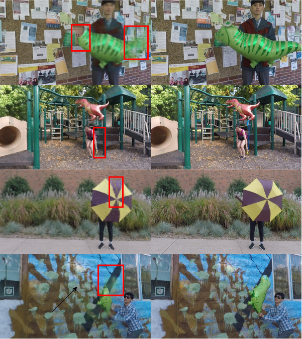
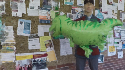
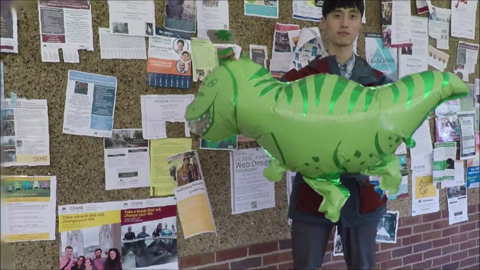
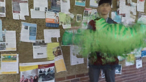
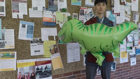
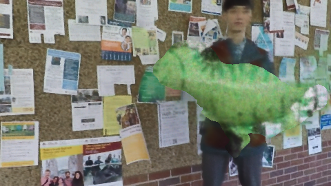
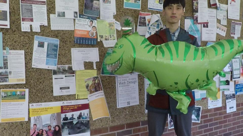
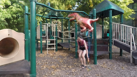
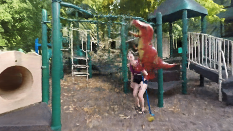
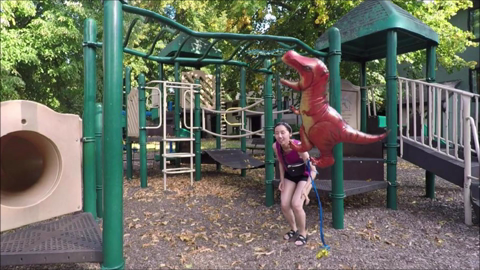
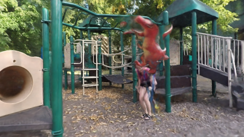
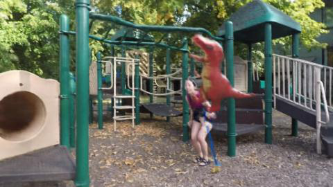
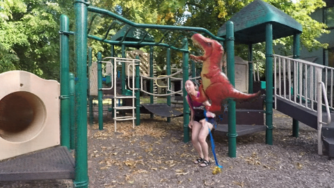
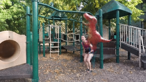
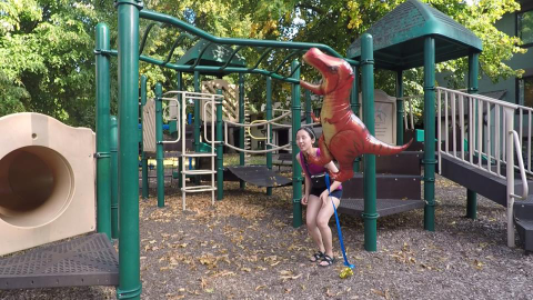
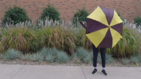
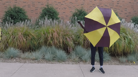
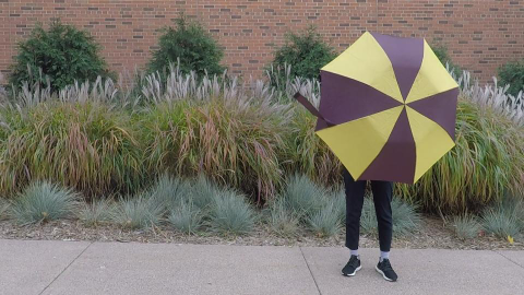
Although we are able to generate realistic outputs in both the novel-view synthesis and the novel-time paradigms, and provide state-of-the-art results, our proposed approach is prone to artifacts due to the extremely unconstrained nature of the tasks. We present some of the failure cases in Figure 6. We address each of the issues from top to bottom, with the ground truth images being displayed on the right-hand side. Balloon1: The artifact on the left is due to improper motion-mask generation, which results in a portion of the dinosaurs head to be cut-off. The artifacts on the right are due to grid errors, which is potentially a by-product of the pixel-pruning step described in section 3.4. Playground: The woman in the image is holding a ribbon extending from the balloon; this ribbon is only partially visible in our reconstruction, we believe that this is caused by the deformation network, which isn’t able to capture the fine detail. The reader may note that other fine objects in the background are represented quite clearly, which indicates that this is most likely caused by incorrect motion-centric modelling. Umbrella: The noticeable streak on the top of the umbrella is caused by pixel-level masking artifacts. Balloon2: The artifact is caused by improper modelling of rigid-body motion at the apex of the balloon’s motion. Most of the identified artifacts are caused by improper blending of motion-centric and background pixels which is an interesting avenue for future research. Although the models are competitive in PSNR values against state-of-the-art models, there remains room for further engineering optimizations to further improve reconstruction rates and overall quality in the future.

5 Conclusion

We present a novel neural radiance-based approach for synthesizing scenes from sparse inputs by modelling both rigid body and non rigid-body motion independently. This approach, coupled with a multi-resolution hash encoding grid, yield state-of-the-art results on the NVIDIA dynamic scenes dataset, while being much faster than existing methods. We also move away from idealized environments and datasets and show the efficacy of our approach on complex real-world scenes, such as the SurgicalActions160 and Cholec80 datasets. We hope that our work leads to widespread adoption of neural radiance-based techniques, and will make our source code publicly available.

6 Supplementary

6.1 Implementation

The code is built on existing repositories and we would like to acknowledge the wonderful contributions made by [37] and [8] for their clean implementation of a fast and modular version of the original NeRF repository [31]. We’d also like to acknowledge the contributions of Muller et al [32, 33] for creating fast CUDA powered kernels and renderers for obtaining excellent speeds during training and inference.

6.2 SurgicalActions160

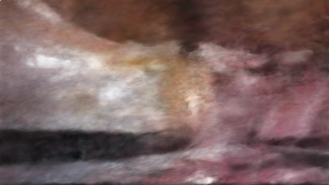
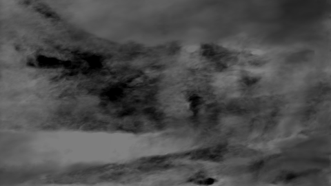
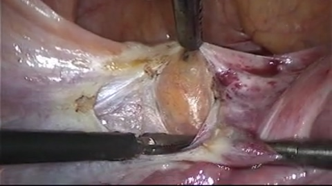
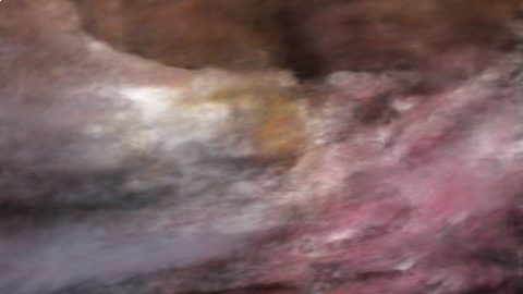
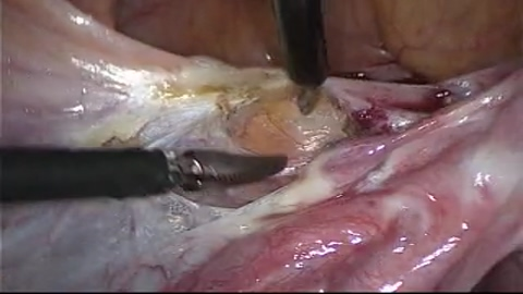
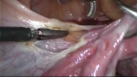
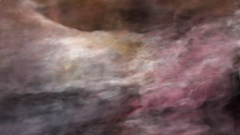
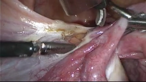
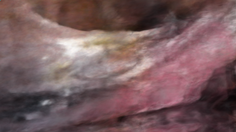
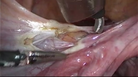
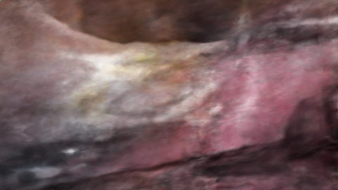
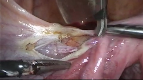
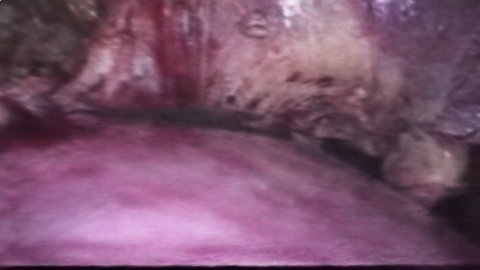
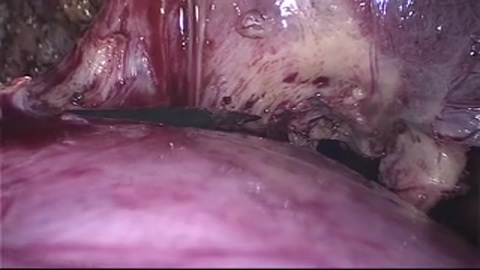
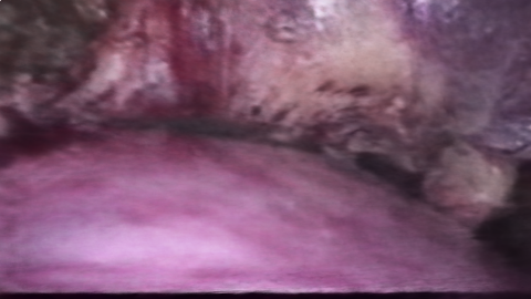
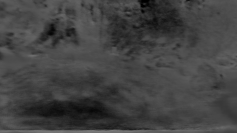
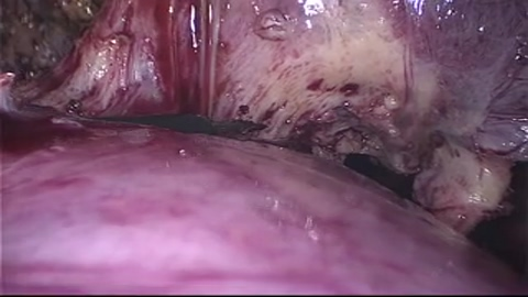
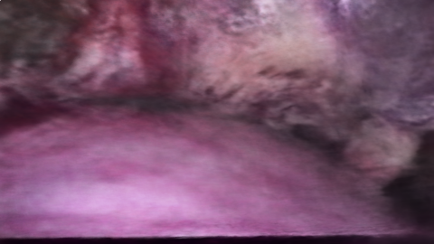
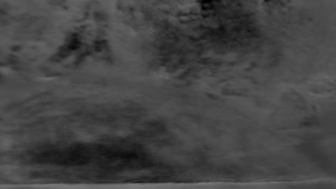
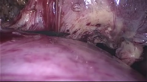
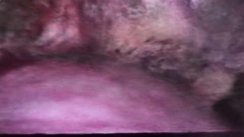
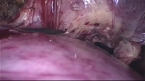
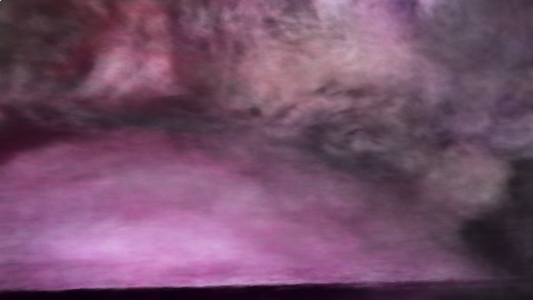
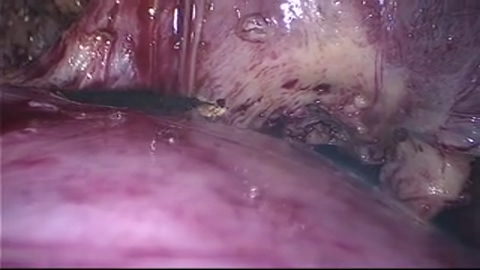
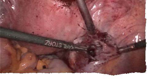
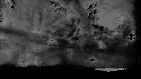
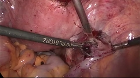
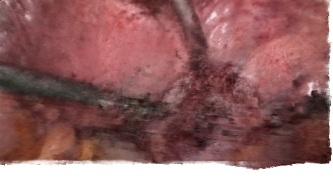
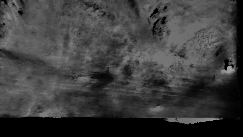
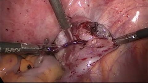
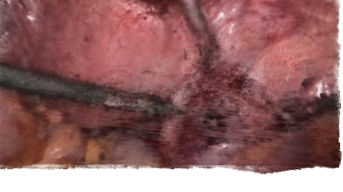
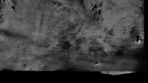
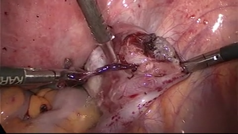
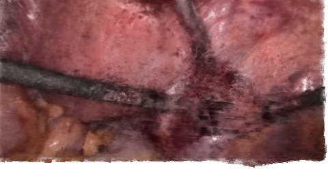
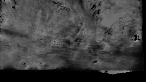
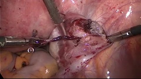
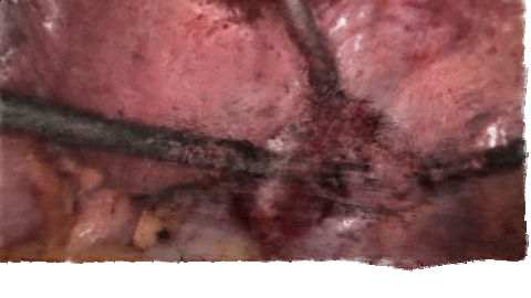
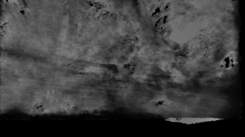
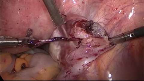
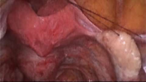
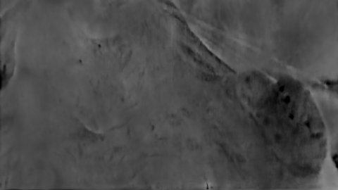
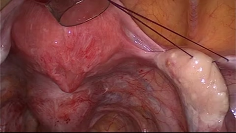
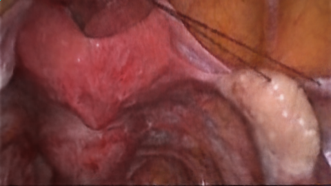
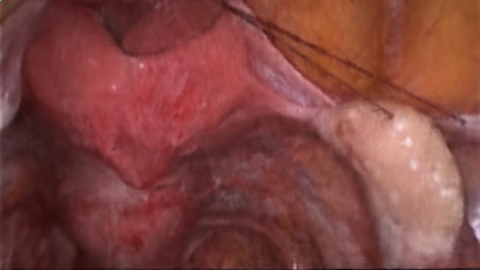
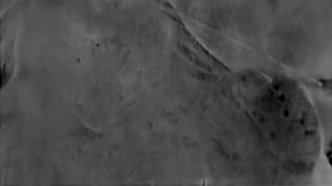
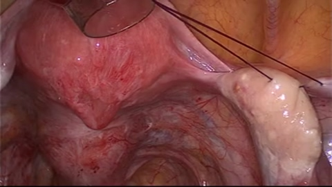
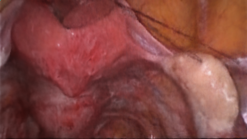
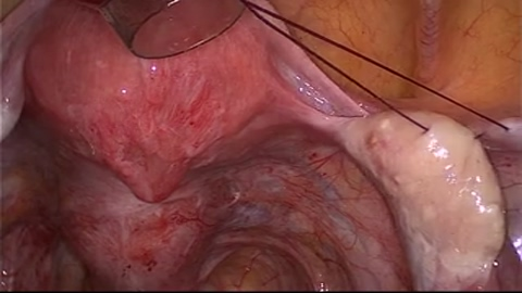
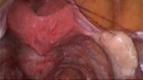
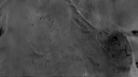
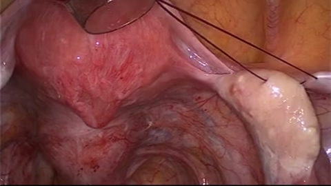
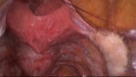
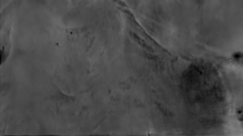
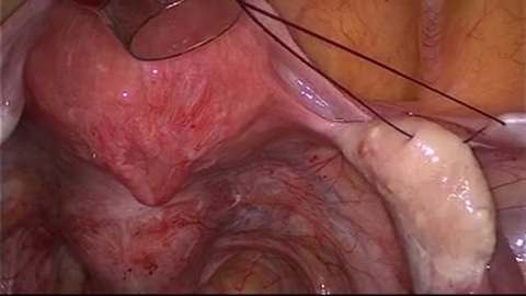
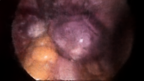
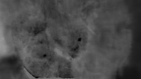
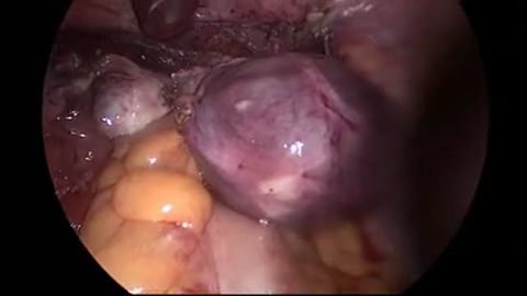
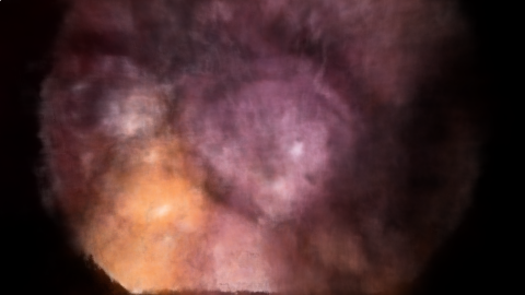
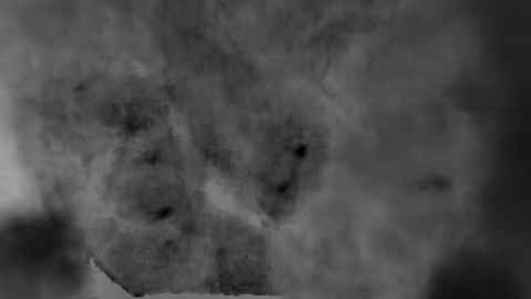
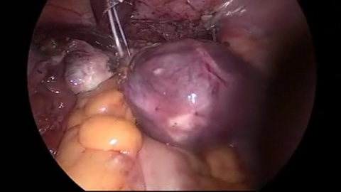
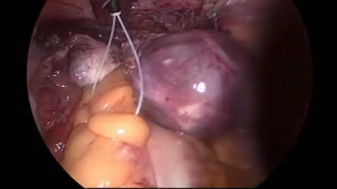
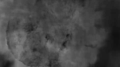
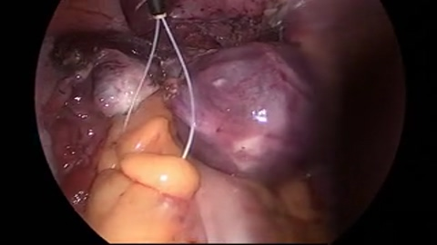
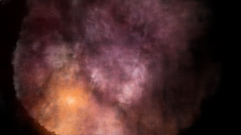
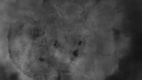
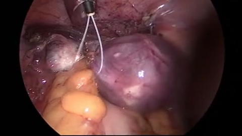
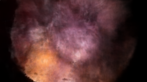
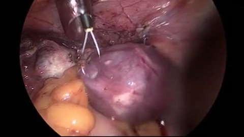
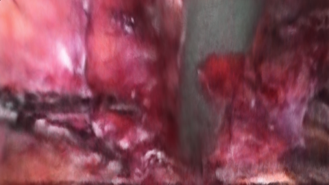
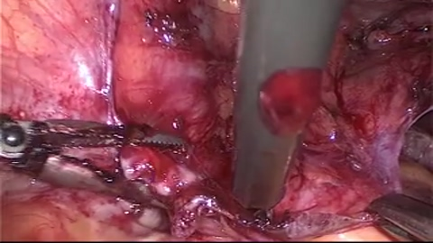
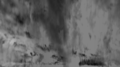
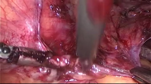
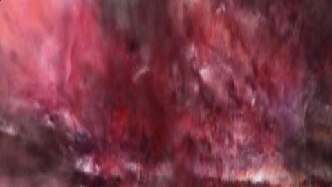
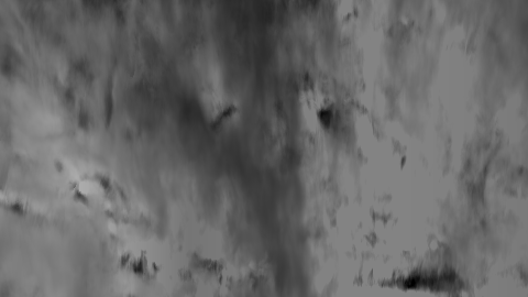
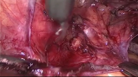
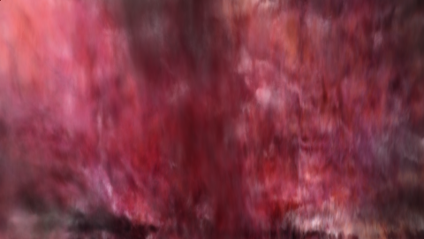
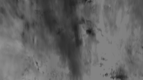
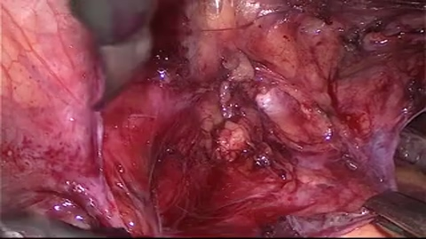
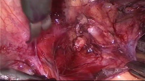
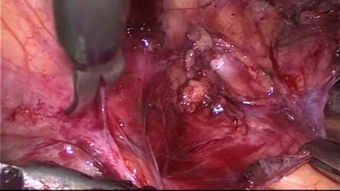
The Surgical Actions dataset consists of 16 different surgical actions and 10 short samples of each. We select the following: Cutting (Figure 13), Blunt dissection (Figure 8), Dissection thermal (Figure 9), Irrigation (Figure 10), Knot-pushing (Figure 11), and Sling-in (Figure 12).

Figure 8: Qualitative results: We present our qualitative results on the SurgicalActions160 dataset, specifically the blunt dissection action. Model reconstructions, Depth predictions, and Ground truth (left to right) - Time-steps (top to bottom)

Figure 9: Qualitative results: We present our qualitative results on the SurgicalActions160 dataset, specifically the dissection thermal action. Model reconstructions, Depth predictions, and Ground truth (left to right) - Time-steps (top to bottom)

Figure 10: Qualitative results: We present our qualitative results on the SurgicalActions160 dataset, specifically the Irrigation action. Model reconstructions, Depth predictions, and Ground truth (left to right) - Time-steps (top to bottom)

Figure 11: Qualitative results: We present our qualitative results on the SurgicalActions160 dataset, specifically the knot-pushing action. Model reconstructions, Depth predictions, and Ground truth (left to right) - Time-steps (top to bottom)

Figure 12: Qualitative results: We present our qualitative results on the SurgicalActions160 dataset, specifically the sling-in action. Model reconstructions, Depth predictions, and Ground truth (left to right) - Time-steps (top to bottom)

Figure 13: Qualitative results: We present our qualitative results on the SurgicalActions160 dataset, specifically the cutting action. Model reconstructions, Depth predictions, and Ground truth (left to right) - Time-steps (top to bottom)

6.3 Cholec80

The inclusion of the Cholec80 dataset is important as it provides an illustration of possible extensions of this method to the extremely challenging datatype - monocular surgical data. We choose only a very short clip extracted from the dataset and show the resulting outputs (Figure 14). For reference, we sub-sample the clips so as to not have to process and thus reconstruct every frame.

Figure 14: Qualitative results: We present our qualitative results on the SurgicalActions160 dataset. Model reconstructions, Depth predictions, and Ground truth (left to right) - Time-steps (top to bottom)

References

- [1] Benjamin Attal, Eliot Laidlaw, Aaron Gokaslan, Changil Kim, Christian Richardt, James Tompkin, and Matthew O’Toole. Törf: Time-of-flight radiance fields for dynamic scene view synthesis. Advances in neural information processing systems, 34:26289–26301, 2021.
- [2] Steven S. Beauchemin and John L. Barron. The computation of optical flow. ACM computing surveys (CSUR), 27(3):433–466, 1995.
- [3] Saifullahi Aminu Bello, Shangshu Yu, Cheng Wang, Jibril Muhmmad Adam, and Jonathan Li. Deep learning on 3d point clouds. Remote Sensing, 12(11):1729, 2020.
- [4] James R Bergen and Edward H Adelson. The plenoptic function and the elements of early vision. Computational models of visual processing, 1:8, 1991.
- [5] Dominique Brunet, Edward R Vrscay, and Zhou Wang. On the mathematical properties of the structural similarity index. IEEE Transactions on Image Processing, 21(4):1488–1499, 2011.
- [6] Thorsten M Buzug. Computed tomography. In Springer handbook of medical technology, pages 311–342. Springer, 2011.
- [7] Julie Chang and Gordon Wetzstein. Deep optics for monocular depth estimation and 3d object detection. In Proceedings of the IEEE/CVF International Conference on Computer Vision, pages 10193–10202, 2019.
- [8] Anpei Chen, Zexiang Xu, Andreas Geiger, Jingyi Yu, and Hao Su. Tensorf: Tensorial radiance fields. arXiv preprint arXiv:2203.09517, 2022.
- [9] Kangle Deng, Andrew Liu, Jun-Yan Zhu, and Deva Ramanan. Depth-supervised nerf: Fewer views and faster training for free. In Proceedings of the IEEE/CVF Conference on Computer Vision and Pattern Recognition, pages 12882–12891, 2022.
- [10] Sara Fridovich-Keil, Alex Yu, Matthew Tancik, Qinhong Chen, Benjamin Recht, and Angjoo Kanazawa. Plenoxels: Radiance fields without neural networks. In Proceedings of the IEEE/CVF Conference on Computer Vision and Pattern Recognition, pages 5501–5510, 2022.
- [11] Chen Gao, Ayush Saraf, Johannes Kopf, and Jia-Bin Huang. Dynamic view synthesis from dynamic monocular video. In Proceedings of the IEEE/CVF International Conference on Computer Vision, pages 5712–5721, 2021.
- [12] Ross Girshick, Ilija Radosavovic, Georgia Gkioxari, Piotr Dollár, and Kaiming He. Detectron, 2018.
- [13] Vitor Guizilini, Rares Ambrus, Sudeep Pillai, Allan Raventos, and Adrien Gaidon. 3d packing for self-supervised monocular depth estimation. In Proceedings of the IEEE/CVF Conference on Computer Vision and Pattern Recognition, pages 2485–2494, 2020.
- [14] Jianfei Guo, Zhiyuan Yang, Xi Lin, and Qingfu Zhang. Template nerf: Towards modeling dense shape correspondences from category-specific object images. arXiv preprint arXiv:2111.04237, 2021.
- [15] Yulan Guo, Hanyun Wang, Qingyong Hu, Hao Liu, Li Liu, and Mohammed Bennamoun. Deep learning for 3d point clouds: A survey. IEEE transactions on pattern analysis and machine intelligence, 43(12):4338–4364, 2020.
- [16] Quan Huynh-Thu and Mohammed Ghanbari. Scope of validity of psnr in image/video quality assessment. Electronics letters, 44(13):800–801, 2008.
- [17] Mohammad Mahdi Johari, Yann Lepoittevin, and François Fleuret. Geonerf: Generalizing nerf with geometry priors. In Proceedings of the IEEE/CVF Conference on Computer Vision and Pattern Recognition, pages 18365–18375, 2022.
- [18] Shuja Khalid, Mitchell Geoffrey Goldenberg, Teodor Pantchev Grantcharov, Babak Taati, and Frank Rudzicz. System and method for surgical performance tracking and measurement, Nov. 26 2020. US Patent App. 16/881,906.
- [19] Shuja Khalid, Vanessa Palter, Teodor Grantcharov, and Frank Rudzicz. Or vision: Objective, explainable assessment of surgical skill with deep learning. 2022.
- [20] Byung-soo Kim, Pushmeet Kohli, and Silvio Savarese. 3d scene understanding by voxel-crf. In Proceedings of the IEEE International Conference on Computer Vision, pages 1425–1432, 2013.
- [21] Katrin Lasinger, René Ranftl, Konrad Schindler, and Vladlen Koltun. Towards robust monocular depth estimation: Mixing datasets for zero-shot cross-dataset transfer. arXiv preprint arXiv:1907.01341, 2019.
- [22] Vincent Lepetit, Pascal Fua, et al. Monocular model-based 3d tracking of rigid objects: A survey. Foundations and Trends® in Computer Graphics and Vision, 1(1):1–89, 2005.
- [23] Zhengqi Li, Simon Niklaus, Noah Snavely, and Oliver Wang. Neural scene flow fields for space-time view synthesis of dynamic scenes. In Proceedings of the IEEE/CVF Conference on Computer Vision and Pattern Recognition, pages 6498–6508, 2021.
- [24] Chen-Hsuan Lin, Wei-Chiu Ma, Antonio Torralba, and Simon Lucey. Barf: Bundle-adjusting neural radiance fields. In Proceedings of the IEEE/CVF International Conference on Computer Vision, pages 5741–5751, 2021.
- [25] Lingjie Liu, Jiatao Gu, Kyaw Zaw Lin, Tat-Seng Chua, and Christian Theobalt. Neural sparse voxel fields. Advances in Neural Information Processing Systems, 33:15651–15663, 2020.
- [26] Shuaicheng Liu, Yinting Wang, Lu Yuan, Jiajun Bu, Ping Tan, and Jian Sun. Video stabilization with a depth camera. In 2012 IEEE Conference on Computer Vision and Pattern Recognition, pages 89–95. IEEE, 2012.
- [27] JN Lyness and BW Ninham. Numerical quadrature and asymptotic expansions. Mathematics of Computation, 21(98):162–178, 1967.
- [28] Julien NP Martel, David B Lindell, Connor Z Lin, Eric R Chan, Marco Monteiro, and Gordon Wetzstein. Acorn: Adaptive coordinate networks for neural scene representation. arXiv preprint arXiv:2105.02788, 2021.
- [29] Ricardo Martin-Brualla, Noha Radwan, Mehdi SM Sajjadi, Jonathan T Barron, Alexey Dosovitskiy, and Daniel Duckworth. Nerf in the wild: Neural radiance fields for unconstrained photo collections. In Proceedings of the IEEE/CVF Conference on Computer Vision and Pattern Recognition, pages 7210–7219, 2021.
- [30] Ben Mildenhall, Peter Hedman, Ricardo Martin-Brualla, Pratul P Srinivasan, and Jonathan T Barron. Nerf in the dark: High dynamic range view synthesis from noisy raw images. In Proceedings of the IEEE/CVF Conference on Computer Vision and Pattern Recognition, pages 16190–16199, 2022.
- [31] Ben Mildenhall, Pratul P Srinivasan, Matthew Tancik, Jonathan T Barron, Ravi Ramamoorthi, and Ren Ng. Nerf: Representing scenes as neural radiance fields for view synthesis. Communications of the ACM, 65(1):99–106, 2021.
- [32] Thomas Müller. Tiny CUDA neural network framework, 2021. https://github.com/nvlabs/tiny-cuda-nn.
- [33] Thomas Müller, Alex Evans, Christoph Schied, and Alexander Keller. Instant neural graphics primitives with a multiresolution hash encoding. arXiv preprint arXiv:2201.05989, 2022.
- [34] Keunhong Park, Utkarsh Sinha, Jonathan T Barron, Sofien Bouaziz, Dan B Goldman, Steven M Seitz, and Ricardo Martin-Brualla. Nerfies: Deformable neural radiance fields. In Proceedings of the IEEE/CVF International Conference on Computer Vision, pages 5865–5874, 2021.
- [35] Keunhong Park, Utkarsh Sinha, Peter Hedman, Jonathan T Barron, Sofien Bouaziz, Dan B Goldman, Ricardo Martin-Brualla, and Steven M Seitz. Hypernerf: A higher-dimensional representation for topologically varying neural radiance fields. arXiv preprint arXiv:2106.13228, 2021.
- [36] Albert Pumarola, Enric Corona, Gerard Pons-Moll, and Francesc Moreno-Noguer. D-nerf: Neural radiance fields for dynamic scenes. In Proceedings of the IEEE/CVF Conference on Computer Vision and Pattern Recognition, pages 10318–10327, 2021.
- [37] Chen Quei-An. Nerf-pl: a pytorch-lightning implementation of nerf, 2020.
- [38] Christian Reiser, Songyou Peng, Yiyi Liao, and Andreas Geiger. Kilonerf: Speeding up neural radiance fields with thousands of tiny mlps. In Proceedings of the IEEE/CVF International Conference on Computer Vision, pages 14335–14345, 2021.
- [39] Barbara Roessle, Jonathan T Barron, Ben Mildenhall, Pratul P Srinivasan, and Matthias Nießner. Dense depth priors for neural radiance fields from sparse input views. In Proceedings of the IEEE/CVF Conference on Computer Vision and Pattern Recognition, pages 12892–12901, 2022.
- [40] Klaus Schoeffmann, Heinrich Husslein, Sabrina Kletz, Stefan Petscharnig, Bernd Muenzer, and Christian Beecks. Video retrieval in laparoscopic video recordings with dynamic content descriptors. Multimedia Tools and Applications, 77(13):16813–16832, 2018.
- [41] Johannes L Schonberger and Jan-Michael Frahm. Structure-from-motion revisited. In Proceedings of the IEEE conference on computer vision and pattern recognition, pages 4104–4113, 2016.
- [42] Katja Schwarz, Axel Sauer, Michael Niemeyer, Yiyi Liao, and Andreas Geiger. Voxgraf: Fast 3d-aware image synthesis with sparse voxel grids. arXiv preprint arXiv:2206.07695, 2022.
- [43] Daeyun Shin, Charless C Fowlkes, and Derek Hoiem. Pixels, voxels, and views: A study of shape representations for single view 3d object shape prediction. In Proceedings of the IEEE conference on computer vision and pattern recognition, pages 3061–3069, 2018.
- [44] Lyne Tchapmi, Christopher Choy, Iro Armeni, JunYoung Gwak, and Silvio Savarese. Segcloud: Semantic segmentation of 3d point clouds. In 2017 international conference on 3D vision (3DV), pages 537–547. IEEE, 2017.
- [45] Zachary Teed and Jia Deng. Raft: Recurrent all-pairs field transforms for optical flow. In European conference on computer vision, pages 402–419. Springer, 2020.
- [46] Edgar Tretschk, Ayush Tewari, Vladislav Golyanik, Michael Zollhöfer, Christoph Lassner, and Christian Theobalt. Non-rigid neural radiance fields: Reconstruction and novel view synthesis of a dynamic scene from monocular video. In Proceedings of the IEEE/CVF International Conference on Computer Vision, pages 12959–12970, 2021.
- [47] Andru P Twinanda, Sherif Shehata, Didier Mutter, Jacques Marescaux, Michel De Mathelin, and Nicolas Padoy. Endonet: a deep architecture for recognition tasks on laparoscopic videos. IEEE transactions on medical imaging, 36(1):86–97, 2016.
- [48] Zirui Wang, Shangzhe Wu, Weidi Xie, Min Chen, and Victor Adrian Prisacariu. Nerf–: Neural radiance fields without known camera parameters. arXiv preprint arXiv:2102.07064, 2021.
- [49] Yi Wei, Shaohui Liu, Yongming Rao, Wang Zhao, Jiwen Lu, and Jie Zhou. Nerfingmvs: Guided optimization of neural radiance fields for indoor multi-view stereo. In Proceedings of the IEEE/CVF International Conference on Computer Vision, pages 5610–5619, 2021.
- [50] Jane Wilhelms and Allen Van Gelder. Octrees for faster isosurface generation. ACM Transactions on Graphics (TOG), 11(3):201–227, 1992.
- [51] Wenxuan Wu, Zhongang Qi, and Li Fuxin. Pointconv: Deep convolutional networks on 3d point clouds. In Proceedings of the IEEE/CVF Conference on Computer Vision and Pattern Recognition, pages 9621–9630, 2019.
- [52] Zhirong Wu, Shuran Song, Aditya Khosla, Fisher Yu, Linguang Zhang, Xiaoou Tang, and Jianxiong Xiao. 3d shapenets: A deep representation for volumetric shapes. In Proceedings of the IEEE conference on computer vision and pattern recognition, pages 1912–1920, 2015.
- [53] Christopher Xie, Keunhong Park, Ricardo Martin-Brualla, and Matthew Brown. Fig-nerf: Figure-ground neural radiance fields for 3d object category modelling. In 2021 International Conference on 3D Vision (3DV), pages 962–971. IEEE, 2021.
- [54] Zexiang Xu, Sai Bi, Kalyan Sunkavalli, Sunil Hadap, Hao Su, and Ravi Ramamoorthi. Deep view synthesis from sparse photometric images. ACM Transactions on Graphics (ToG), 38(4):1–13, 2019.
- [55] Junlan Yang, Dan Schonfeld, and Magdi Mohamed. Robust video stabilization based on particle filter tracking of projected camera motion. IEEE Transactions on Circuits and Systems for Video Technology, 19(7):945–954, 2009.
- [56] Jae Shin Yoon, Kihwan Kim, Orazio Gallo, Hyun Soo Park, and Jan Kautz. Novel view synthesis of dynamic scenes with globally coherent depths from a monocular camera. In Proceedings of the IEEE/CVF Conference on Computer Vision and Pattern Recognition, pages 5336–5345, 2020.
- [57] Alex Yu, Ruilong Li, Matthew Tancik, Hao Li, Ren Ng, and Angjoo Kanazawa. Plenoctrees for real-time rendering of neural radiance fields. In Proceedings of the IEEE/CVF International Conference on Computer Vision, pages 5752–5761, 2021.
- [58] Richard Zhang, Phillip Isola, Alexei A Efros, Eli Shechtman, and Oliver Wang. The unreasonable effectiveness of deep features as a perceptual metric. In Proceedings of the IEEE conference on computer vision and pattern recognition, pages 586–595, 2018.
- [59] Xingyi Zhou, Vladlen Koltun, and Philipp Krähenbühl. Tracking objects as points. In European Conference on Computer Vision, pages 474–490. Springer, 2020.
- [60] Yin Zhou and Oncel Tuzel. Voxelnet: End-to-end learning for point cloud based 3d object detection. In Proceedings of the IEEE conference on computer vision and pattern recognition, pages 4490–4499, 2018.