Momentum Adversarial Distillation: Handling Large Distribution Shifts in Data-Free Knowledge Distillation

Abstract

Data-free Knowledge Distillation (DFKD) has attracted attention recently thanks to its appealing capability of transferring knowledge from a teacher network to a student network without using training data. The main idea is to use a generator to synthesize data for training the student. As the generator gets updated, the distribution of synthetic data will change. Such distribution shift could be large if the generator and the student are trained adversarially, causing the student to forget the knowledge it acquired at previous steps. To alleviate this problem, we propose a simple yet effective method called Momentum Adversarial Distillation (MAD) which maintains an exponential moving average (EMA) copy of the generator and uses synthetic samples from both the generator and the EMA generator to train the student. Since the EMA generator can be considered as an ensemble of the generator’s old versions and often undergoes a smaller change in updates compared to the generator, training on its synthetic samples can help the student recall the past knowledge and prevent the student from adapting too quickly to new updates of the generator. Our experiments on six benchmark datasets including big datasets like ImageNet and Places365 demonstrate the superior performance of MAD over competing methods for handling the large distribution shift problem. Our method also compares favorably to existing DFKD methods and even achieves state-of-the-art results in some cases.

1 Introduction

With the development of deep learning, more pretrained deep neural networks have been released to the public [5, 10, 18, 38, 43]. However, their superior performances often come with big sizes, causing difficulties in deployment of these pretrained networks on resource-constrained devices. This leads to the demand for transferring knowledge from a cumbersome pretrained source network (called “teacher”) to a compact target network (called “student”) with a minimal loss of performance. This task is regarded as Knowledge Distillation (KD) [19].

The original idea of KD is to make use of class probabilities predicted by the teacher which encapsulate the hidden correlation among classes as training signals for the student. Note that such “dark” knowledge [19] is generally not available if the student is trained directly on raw data with one-hot labels. Later, various KD methods have been proposed to improve the quality of knowledge transfer. For example, AT [47] matches the spatial attention maps at intermediate layers of the student and the teacher. SPD [42] encourages the similarity between the student’s and teacher’s feature correlation matrices. PKT [36] transfers the conditional probability between two samples computed via kernel density estimation on the feature space. RKD [35] exploits relational knowledge for distillation. VID [1] maximizes a variational lower bound of the mutual information (MI) between the student’s and teacher’s representations. CRD [41] uses contrastive learning as a proxy for maximizing MI.

The common drawback of these methods is the reliance on samples from the teacher training set. However, in practice, accessing the original training data is usually infeasible due to many reasons such as data privacy (e.g., healthcare data containing personal information) or data regarded as intellectual property of the vendors. Addressing this critical issue, Data-Free Knowledge Distillation (DFKD) methods have been introduced [7, 13, 27, 29, 31, 34, 44, 45, 46]. A common DFKD approach is to use a generator network to synthesize training data and jointly train the generator and the student in an adversarial manner [13, 31, 46]. Under this adversarial learning scheme, the student attempts to make predictions as close as possible to the teacher’s on synthetic data generated by the generator, while the generator tries to create samples that maximize the mismatch between the student’s and the teacher’s predictions. This adversarial game enables a rapid exploration of synthetic distributions useful for knowledge transfer between the teacher and the student. At the same time, it could also lead to large shifts in the synthetic distributions, causing the student to forget useful knowledge acquired at the previous steps and suffer from performance drops [3].

In this paper, we propose a simple yet effective method called Momentum Adversarial Distillation (MAD) to mitigate the large distribution shift problem in adversarial DFKD. MAD maintains an exponential moving average (EMA) copy of the generator which is responsible for storing information about past updates of the generator. By using synthetic samples from the EMA generator as additional training data for the student besides those from the generator, MAD can ensure that the student can recall the old knowledge, hence, is less prone to forgetting. Moreover, to reduce the negative effect caused by spurious solutions of an unconditional generator when learning on large datasets such as ImageNet, we propose to use a class-conditional generator that takes the sum of a noise vector and a class embedding vector as input, and train this generator with a new objective that suppresses the presence of spurious solutions. This technique requires only a small change in the generator’s architecture but enables MAD (and possibly other adversarial DFKD methods) to learn surprisingly well on large datasets. Through extensive experiments on three small and three large image datasets, we demonstrate that our proposed method is far better than related baselines [3, 31] in dealing with the large distribution shift problem. In some cases, MAD even outperforms current state-of-the-art methods [8, 14].

2 Adversarial Data-Free Knowledge Distillation

Let $\mathtt{T}$ be a teacher network pretrained on some dataset $\mathcal{D}_{\text{train}}$ and $\mathtt{S}$ be a fresh student network. Let $\mathtt{T}(\cdot)$ and $\mathtt{S}(\cdot)$ denote outputs of the teacher and student networks before the softmax activation, respectively. In Data-Free Knowledge Distillation (DFKD), we want to transfer knowledge from $\mathtt{T}$ to $\mathtt{S}$ so that $\mathtt{S}$ performs as well as or even better than $\mathtt{T}$ on the original test set $\mathcal{D}_{\text{test}}$ but with a constraint that no training data for $\mathtt{S}$ is available. An intuitive way to deal with such constraint is learning an additional generator network $\mathtt{G}$ that can generate synthetic data for training $\mathtt{S}$ from a noise distribution $p(z)$ usually chosen to be the standard Gaussian distribution $\mathcal{N}(0,\mathrm{I})$. Adversarial Belief Matching (ABM) [31] proposed an adversarial learning framework between $\mathtt{S}$ and $\mathtt{G}$ via optimizing the following min-max objective:

$$\min_{\mathtt{S}}\max_{\mathtt{G}}\mathbb{E}_{z\sim p(z)}\left[\mathcal{L}_{\text{KD}}(\mathtt{G}(z))\right]$$ (1)

$$\Leftrightarrow \min_{\mathtt{S}}\max_{\mathtt{G}}\mathbb{E}_{z\sim p(z),x=\mathtt{G}(z)}\left[\mathcal{L}_{\text{KD}}(x)\right],$$ (2)

where $\mathcal{L}_{\text{KD}}(x)$ denotes the knowledge distillation (KD) loss, i.e., the discrepancy between $\mathtt{S}(x)$ and $\mathtt{T}(x)$. In ABM, $\mathcal{L}_{\text{KD}}(x)$ is the Kullback-Leibler (KL) divergence between class probabilities of $\mathtt{T}$ and $\mathtt{S}$ computed on $x$:

$$\mathcal{L}_{\text{KD}}(x) \triangleq D_{\text{KL}}\left(\mathtt{Tp}(x)\|\mathtt{Sp}(x)\right)=\sum_{c=1}^{C}\mathtt{Tp}(x)[c]\cdot\left(\log\mathtt{Tp}(x)[c]-\log\mathtt{Sp}(x)[c]\right),$$ (3)

where $\mathtt{Tp}(x)=\text{softmax}(\mathtt{T}(x))$ and $\mathtt{Sp}(x)=\text{softmax}(\mathtt{S}(x))$ denote the class probabilities of $\mathtt{T}$ and $\mathtt{S}$ computed on $x$, respectively; and $C$ is the total number of classes.

The core idea behind the optimization in Eq. 1 is to encourage $\mathtt{G}$ to generate samples on which the outputs of $\mathtt{S}$ are very different from those of $\mathtt{T}$ (or the KD loss is large). Typically, the generated samples have not been observed by $\mathtt{S}$ during training (otherwise, the KD loss will be small) and the learning task of $\mathtt{S}$ is to match $\mathtt{T}$ on these novel samples. It is expected that in the ideal case, via continuous adversarial exploration of $\mathtt{G}$, $\mathtt{S}$ can be exposed to a diverse enough set of synthetic samples which allows $\mathtt{S}$ to match $\mathtt{T}$ with an arbitrarily small prediction error on $\mathcal{D}_{\text{test}}$.

In practice, we usually implement Eq. 1 by alternately optimizing $\mathtt{S}$ and $\mathtt{G}$ in $n_{\mathtt{S}}$ and $n_{\mathtt{G}}$ steps, respectively. Thus, to avoid confusion later, we refer to a $n_{\mathtt{S}}$-step update of $\mathtt{S}$ as an update stage of $\mathtt{S}$ and similarly, a $n_{\mathtt{G}}$-step update of $\mathtt{G}$ as an update stage of $\mathtt{G}$.

3 Momentum Adversarial Distillation

Figure 1: An illustration of our proposed Momentum Adversarial Distillation (MAD) consisting of a teacher ($\mathtt{T}$), a student ($\mathtt{S}$), a class-conditional generator ($\mathtt{G}$), an EMA generator ($\tilde{\mathtt{G}}$), and class embeddings ($\mathtt{E}$). Networks with dashed borders ($\mathtt{T}$, $\tilde{\mathtt{G}}$) are not optimized during training. $z$ and $z^{\prime}$ are random noises sampled from $\mathcal{N}(0,\mathrm{I})$. $e_{y}$ and $e_{y^{\prime}}$ are gathered from $\mathtt{E}$ at index $y$ and $y^{\prime}$, respectively.

3.1 Handling large distribution shifts with an additional EMA generator

Although theoretically sound, the optimization in Eq. 1 has a practical problem: If the update of $\mathtt{G}$ varies too much, the distribution of synthetic samples generated by $\mathtt{G}$ will change significantly over two consecutive update steps of $\mathtt{S}$, which in turns causes $\mathtt{S}$ to catastrophically forget what it has learned at the previous stages [3] to adapt to the new update of $\mathtt{G}$. In order to address this problem, we propose to maintain an exponential moving average (EMA) of the generator $\mathtt{G}$, denoted by $\tilde{\mathtt{G}}$, during learning and use synthetic samples from both $\mathtt{G}$ and $\tilde{\mathtt{G}}$ to train $\mathtt{S}$ as follows:

$$\min_{\mathtt{S}}\mathcal{L}_{\mathtt{S}}\triangleq\lambda_{0}\mathbb{E}_{z\sim p(z)}\left[\mathcal{L}_{\text{KD}}(\mathtt{G}(z))\right]+\lambda_{1}\mathbb{E}_{z^{\prime}\sim p(z)}\left[\mathcal{L}_{\text{KD}}(\tilde{\mathtt{G}}(z^{\prime}))\right],$$ (4)

where $\lambda_{0},\lambda_{1}\geq 0$ are coefficients. The parameters $\theta_{\tilde{\mathtt{G}}}^{t}$ of the momentum generator $\tilde{\mathtt{G}}$ at the update stage $t$ of $\mathtt{S}$ (after $n_{\mathtt{G}}$ steps update of $\mathtt{G}$) are computed as:

$$\theta_{\tilde{\mathtt{G}}}^{t}=\alpha\cdot\theta_{\tilde{\mathtt{G}}}^{t-1}+(1-\alpha)\cdot\theta_{\mathtt{G}}^{t},$$ (5)

where $\alpha$ ($0<\alpha<1$) is the momentum. If $\alpha$ is close to 1, $\tilde{\mathtt{G}}$ will change very slightly compared to $\mathtt{G}$. Therefore, by using synthetic samples from $\tilde{\mathtt{G}}$ as additional training data for $\mathtt{S}$ besides those from $\mathtt{G}$, we can alleviate the large exploratory distribution shift caused by the large update of $\mathtt{G}$ and achieve a stable update of $\mathtt{S}$. We name our proposed method Momentum Adversarial Distillation (MAD). See Fig. 1 for an illustration.

3.2 Enabling MAD to learn well on large datasets

During our experiments, we observed that MAD, with the unconditional generator $\mathtt{G}$ described in Section 2, is not able to learn well on large datasets such as ImageNet. Our hypothesis is that in case of large datasets, the objective of $\mathtt{G}$ in Eq. 2 induces a very large number spurious solutions, which hampers the learning of $\mathtt{G}$. To see this, first let us recall the objective of $\mathtt{G}$ which is maximizing the KL divergence between $\mathtt{Sp}(x)$ and $\mathtt{Tp}(x)$ over some synthetic sample $x=\mathtt{G}(z)$. If we, for example, assume that there are 3 classes in total and $\mathtt{Tp}(x)$ is fixed at $[1,0,0]$, then we could train $\mathtt{G}$ to generate $x$ so that $\mathtt{Sp}(x)$ is either $[0,1,0]$ or $[0,0,1]$. In this toy example, we see 2 spurious solutions for 3 classes. If a dataset has 1000 classes like ImageNet, there will be at least 999 spurious solutions. Besides class numbers, larger input sizes also increase the space and the number of (spurious) solutions. Unfortunately, the more spurious solutions, the more likely $\mathtt{G}$ could jump from one spurious solution to another in successive update steps, causing instability in training $\mathtt{G}$.

To overcome this problem, we propose to condition $\mathtt{G}$ on a class label $y$ as $\mathtt{G}(z+e_{y})$ where $e_{y}$ is a trainable embedding of $y$. We found that using the sum of $z$ and $e_{y}$ as input to $\mathtt{G}$ instead of concatenation allows our method to learn much better, possibly because the noise in updating $e_{y}$ is absorbed into the stochasticity of $z$ via summation rather than concatenation. We illustrate this idea in Fig. 1, and provide an empirical justification in Appdx. B.3. Denoted by $\mathtt{E}$ the list of trainable embedding vectors for all classes ($\mathtt{E}=(e_{1},...,e_{C})$), we train both $\mathtt{G}$ and $\mathtt{E}$ together by minimizing the following loss:

$$\min_{\mathtt{G},\mathtt{E}}\mathcal{L}_{\mathtt{G},\mathtt{E}}\triangleq\mathbb{E}_{z\sim\mathcal{N}(0,\mathrm{I}),y\sim\text{Cat}(C),x=\mathtt{G}(z+e_{y})}\left[-\lambda_{2}\mathcal{L}_{\text{KD}}(x)+\lambda_{3}\mathcal{L}_{\text{NLL}}(x,y)+\lambda_{4}\mathcal{L}_{\text{NormReg}}(e_{y})\right],$$ (6)

where $\text{Cat}(C)$ is the uniform categorical distribution over $C$ classes; $\lambda_{2},\lambda_{3},\lambda_{4}\geq 0$ are hyperparameters; and $\mathcal{L}_{\text{NLL}}(x,y)$ and $\mathcal{L}_{\text{NormReg}}(e_{y})$ are the negative log-likelihood and the norm regularization losses respectively, defined as follows:

$$\mathcal{L}_{\text{NLL}}(x,y) \triangleq-\log\mathtt{Tp}(x)[y],$$ (7)

$$\mathcal{L}_{\text{NormReg}}(e_{y}) \triangleq\max\left({\left\|e_{y}\right\|}_{2}-\gamma\times\sqrt{d_{e}},0\right),$$ (8)

where $d_{e}$ denotes the dimensionality of $e_{y}$; and $\gamma\geq 1$ is a scaling hyperparameter. $\mathcal{L}_{\text{NormReg}}(e_{y})$ servers as a constraint that restricts the norm of $e_{y}$ to be smaller than $\gamma\times\sqrt{d_{e}}$. An explanation of the formula $\gamma\times\sqrt{d_{e}}$ is provided in Appdx. C. Intuitively, via minimizing $\mathcal{L}_{\text{NLL}}(x,y)$, $\mathtt{G}$ could maintain its focus on predicting $y$ throughout its entire update stage rather than jumping between different spurious solutions. Besides, since $y$ is sampled uniformly, the synthetic data will be evenly distributed among classes.

In case the teacher $\mathtt{T}$ has BatchNorm [20] layers, we can make use of the running mean $\bar{\mu}_{\ell}$ and running variance $\bar{\omega}_{\ell}$ of each BatchNorm layer $\ell$ of $\mathtt{T}$ to guide the data synthesis of $\mathtt{G}$ by adding the BatchNorm moment matching (BNmm) loss [45] below to $\mathcal{L}_{\mathtt{G},\mathtt{E}}$ (weighted by $\lambda_{5}\geq 0$):

$$\mathcal{L}_{\text{BNmm}}\triangleq\sum_{\ell}\left\|\mu_{\ell}-\bar{\mu}_{\ell}\right\|_{2}^{2}+\left\|\omega_{\ell}-\bar{\omega}_{\ell}\right\|_{2}^{2},$$ (9)

where $\mu_{\ell}$, $\omega_{\ell}$ are the empirical mean and variance of the features at the BatchNorm layer $\ell$ w.r.t. the batch of synthetic samples from $\mathtt{G}$. During our experiment, we observed that using $\mathcal{L}_{\text{BNmm}}$ improves knowledge distillation of the student $\mathtt{S}$.

4 Related Work

In Data-Free Knowledge Distillation (DFKD), it is critical to synthesize data that are useful for transferring knowledge from $\mathtt{T}$ to $\mathtt{S}$. Existing DFKD methods differ mainly in their objectives to guide the data synthesis. These methods generally fall into either the adversarial camp or the non-adversarial camp. Non-adversarial DFKD methods [7, 27, 29, 34, 44, 46] make use of certain heuristics to search for synthetic data that resembles the original training data $\mathcal{D}_{\mathtt{T},\text{train}}$. For example, ZSKD [34] and DAFL [7] consider prediction probabilities of $\mathtt{T}$ and the confidence of $\mathtt{T}$ as heuristics. In DAFL, synthetic data is generated via a generator $\mathtt{G}$ rather than being optimized directly like in ZSKD. KegNet [46] extends DAFL by making $\mathtt{G}$ conditioned on class labels. Adversarial DFKD methods [8, 14, 17, 37, 45, 50] leverage adversarial learning to explore the data space more efficiently. Most methods of this type are derived from the ABM [31] discussed in Section 2 with additional objectives to improve the quality and/or diversity of synthetic data. For example, RDSKD [17] uses a diversity-seeking loss [30]; CMI [14] uses an inverse contrastive loss to improve diversity; and DeepInversion [45] uses Batch Norm moment matching (BNmm) and DeepDream’s inception losses (total variation, L2) [32] to generate visually interpretable images.

DeepInversion [45] is one of a few DFKD methods [12, 29, 45] that have been shown to learn well on the full-size ImageNet dataset. Its success has inspired subsequent works on large-scale continual learning [39] and data-free object detection [6]. However, training DeepInversion on ImageNet is very time-consuming because this method optimizes synthetic images directly and each complete optimization requires a very large number of iterations (about 20,000). LS-GDFD [29] learns to generate synthetic data instead but requires one generator for each class (that is, 1,000 generators for 1,000 classes) to avoid the “mode collapse” problem and achieve good performance. FastDFKD [12] leverages meta-learning to speed up the training process significantly. On the contrary, by applying our proposed technique in Section 3.2, our MAD only needs 1 generator (compared to 1,000 of LS-GDFD) and 6,000 training iterations (compared to 20,000$\times$ of DeepInversion) to achieve reasonably good performance on ImageNet (Section 5.2.2). In addition, our technique is orthogonal to and can combine with the meta-learning idea in [12] for further improvement.

Besides the DFKD methods discussed above, there is a line of works that consider a less extreme scenario in which unlabeled transfer sets are given for training. These transfer sets can be very different from the original dataset in terms of distribution and semantics and can be freely collected from open resources. Nayak et al. [33] analyzed various kinds of transfer sets ranging from random noise images to natural images and found that the target-class balance property of the transfer set and the similarity between the transfer set and the original training set play important roles in improving knowledge distillation results. Fang et al. [11] argued that although the transfer images can be semantically different from the original traning images, they still share common local visual patterns. Therefore, the authors proposed an interesting method called MosaicKD which combines different local patches extracted from the transfer images to craft synthetic mosaic images that capture the semantics of the original data while enjoy realistic local structures.

Adversarial training methods like GANs has been shown to suffer from the catastrophic forgetting problem of the discriminator [26, 40]. These works consider GANs training as a continual learning problem and leverage existing methods to mitigate the issue. For example, Liang et al. [26] use either EWC [23] or SI [49] to enforce similarity between the discriminator’s weights at the current step and at the last checkpoint. Hoang et al. [40] suggest some other tricks such as using a momentum optimizer (e.g., Adam [21]) or applying gradient penalty [16] to the discriminator. In this paper, we consider the catastrophic forgetting problem of the student as a consequence of the large distribution shift problem caused by the generator. Therefore, we focus on regularizing the generator rather than the student. Besides, from this perspective, the catastrophic forgetting problem in GANs is indeed less severe than that in adversarial DFKD. It is because in GANs, the discriminator is trained on real data with a fixed distribution, which can somewhat reduce the effect of the distribution shift of fake (synthetic) data while in adversarial DFKD, real data is not available. Recent works that also address the student forgetting problem in DFKD like ours include DFKD-Mem [3] and PRE-DFKD [2]. DFKD-Mem [3] stores the past synthetic samples in a memory bank and uses these samples as additional training data for the student. Our method, on the other hand, uses an EMA generator to generate old synthetic samples on-the-fly, which is more memory efficient and adapts better to the student update. PRE-DFKD [2] models past synthetic data via a VAE [22] and treats the decoder of this VAE as a replay generator. However, training a VAE on a continuous stream of synthetic samples could be unstable and could lead to another catastrophic forgetting problem on its own. In addition, VAE is not effective for generating images with large size (e.g., ImageNet images) due to the “posterior collapse” problem [28].

5 Experiments

5.1 Experimental Setup

Datasets

We consider the image classification task and evaluate our proposed method on 3 small image datasets (CIFAR10 [24], CIFAR100 [24], TinyImageNet [25]), and 3 large image datasets (ImageNet [9], Places365 [51], Food101 [4]). Details are provided in Appdx. A.1.

Network architectures

For the small datasets, we follow [8, 14] and consider ResNet34/ResNet18 [18] and WRN40-2/WRN16-2 [48] for the teacher/student. We observed that knowledge distillation with the WRN architectures is more challenging than with the ResNet architectures, possibly because WRN40-2/WRN16-2 have much fewer parameters than ResNet34/ResNet18. For the large datasets, we use the AlexNet architecture for both the teacher and student for fast training. Since AlexNet does not have any BatchNorm layer, we exclude the BNmm loss (Eq. 9) from the total loss of the generator in our experiments on the large datasets. Architectures of the generator w.r.t. different datasets are given in Appdx. A.4.

Training settings of teacher

For ImageNet, we make use of pretrained networks provided by PyTorch. For other datasets, we train the teacher from scratch. Detailed training settings of the teacher are given in Appdx. A.2.

Training settings of MAD

If not otherwise specified, we set the momentum $\alpha$ in Eq. 5 to $0.95$ and the length of the noise vector to 256. We train the student $\mathtt{S}$ using SGD and Adam for the small and large datasets, respectively. We train the generator $\mathtt{G}$ using Adam for both the small and large datasets. To reduce the difficulty of training $\mathtt{G}$ for the large datasets, we pretrain $\mathtt{G}$ for some steps before the main KD training by setting the coefficient of $\mathcal{L}_{\text{KD}}$ to 0 and only optimizing the remaining losses in Eq. 6. The generator $\mathtt{G}$ is class-conditional (as described in Section 3.2) for the large datasets, and unconditional for the small datasets. We empirically found that this leads to better results. For further details about the training settings of MAD, please refer to Appdx. A.3.

5.2 Results

5.2.1 Comparison with existing DFKD methods

In Table 5.2.1, we compare MAD with existing DFKD methods [7, 8, 13, 14, 34, 45, 50] on the small datasets. The results of baselines are taken from [14, 50]. We checked the results of the teacher trained by us and found that they are quite similar to the results of the teacher reported in [14] and in Table 5.2.1 (details in Appdx. B.1). This means our results of MAD are comparable with those of the baselines. We see that MAD outperforms all the DFKD methods on CIFAR10 and CIFAR100 in case the teacher and student are ResNets [18] ($\heartsuit$). In case the teacher and student are WideResNets [48] ($\diamondsuit$), our method still achieves significantly better results than most of the baselines such as DAFL [7] and ZSKT [34] and only performs worse than CMI [14]. We hypothesize it is mainly because of the differences in model design and training settings of CMI and MAD. For example, CMI has an additional contrastive-loss-based objective that encourages the generator’s diversity while MAD does not. CMI also performs more updates of the student and generator per training step than our method.

However, our ultimate goal for this section is not to show that MAD can achieve state-of-the-art results in all cases (which often requires intensive hyper-parameter tuning) but to verify the soundness of our implementation of MAD. In order to see clearly the advantage of MAD, we need to compare MAD with its related baselines under the same settings. This will be presented in Section 5.2.2.

Dataset	Arch.	Tea.a	Stu.a	DAFLa	ZSKTa	ADIa	DFADb	DDADb	DFQa	CMIa	MAD
CIFAR10	$\heartsuit$	95.70	95.20	92.22	93.32	93.26	93.30	94.81	94.61	94.84	94.90
	$\diamondsuit$	94.87	93.95	81.55	89.66	89.72	-	-	92.01	92.52	92.64
CIFAR100	$\heartsuit$	78.05	77.10	74.47	67.74	61.32	69.43	75.04	77.01	77.04	77.31
	$\diamondsuit$	75.83	73.56	40.00	28.44	61.34	-	-	59.01	68.75	64.05
TinyIN	$\heartsuit$	66.44	64.87	-	-	-	-	-	63.73	64.01	62.32

Table 1: Classification accuracy (in %) of the student trained by different DFKD methods on 3 small image datasets. The teacher/student architecture settings are ResNet34/ResNet18 ($\heartsuit$) and WRN40-2/WRN16-2 ($\diamondsuit$). ^a and ^b denote results taken from [14] and [50], respectively. Tea. and Stu. denote the teacher and student trained from scratch on $\mathcal{D}_{\text{train}}$. The best and second best results are highlighted in bold and italic, respectively.

5.2.2 Comparison with related baselines

We consider two related baselines of MAD which are ABM [31] and DFKD-Mem [3]. ABM learns the student $\mathtt{S}$ with only synthetic samples from $\mathtt{G}$. DFKD-Mem, on the other hand, stores past synthetic samples in a memory bank, and uses samples from this memory bank (dubbed “memory samples”) as well as those generated by $\mathtt{G}$ as training data for $\mathtt{S}$. We trained ABM and DFKD-Mem using exactly the same settings for training MAD. For DFKD-Mem, we set the memory size to 8,192. For other memory sizes, the results remain relatively similar as shown in Appdx. B.2.

From Table 2 and Fig. 2, it is clear that MAD significantly outperforms both ABM and DFKD-Mem on all datasets. In addition, the performance gaps between our method and the two baselines tend to be larger for larger datasets. For example, MAD achieves about 1.5/2.8%, 2.5/3.6%, and 4.2/2.2% higher accuracy than ABM/DFKD-Mem on CIFAR100, TinyImageNet, and ImageNet, respectively. These empirical results suggest the importance of the EMA generator $\tilde{\mathtt{G}}$ in mitigating the large distribution shift caused by $\mathtt{G}$.

In this experiment, we found that DFKD-Mem often performs worse than ABM on CIFAR100 and TinyImageNet. We found the decay of the student learning rate is the main reason for this. As shown in Fig. 3a, the distillation loss on memory samples surges when the (student) learning rate is decayed and cannot recover if the new learning rate is too small ($lr_{\mathtt{S}}$ = 1e-4), which is in contrast to the distillation loss on synthetic samples from $\mathtt{G}$ or $\tilde{\mathtt{G}}$ (Figs. 3b,3c). This implies a potential issue of storing old samples in a memory bank instead of using the EMA generator as memory samples could be completely out-of-date if the student suddenly change its state (e.g., via learning rate decay). However, even when the learning rate does not change (e.g., from step 0 to step 100 on CIFAR100 or on ImageNet/Places365), DFKD-Mem still performs worse than our method.

Dataset	CIFAR10	CIFAR100	TinyIN	ImageNet	Places365	Food101
Arch.	$\diamondsuit$	$\diamondsuit$	$\heartsuit$	$\clubsuit$	$\clubsuit$	$\clubsuit$
Teacher	94.65	75.65	66.47	56.52	50.80	65.15
ABM	92.38	62.59	59.75	41.23	41.84	60.37
DFKD-Mem	92.09	61.25	58.66	43.30	42.38	61.25
MAD	92.64	64.05	62.32	45.48	43.67	61.74

Table 2: Classification accuracy (in %) of MAD and its related baselines on 3 small and 3 large image datasets. The teacher/student architecture settings are ResNet34/ResNet18 ($\heartsuit$), WRN40-2/WRN16-2 ($\diamondsuit$), and AlexNet/AlexNet ($\clubsuit$). The teacher’s results are from our own runs (Appdx. B.1). The best results are highlighted in bold.

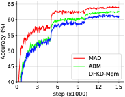
(a) CIFAR100

(b) TinyImageNet

(c) ImageNet

(d) Places365

Figure 2: Test accuracy curves of $\mathtt{S}$ trained via MAD, ABM, and DFKD-Mem on some datasets.

(a) $\mathcal{L}_{\text{KD}}$ on memory samples

(b) $\mathcal{L}_{\text{KD}}$ on samples from $\mathtt{G}$

(c) $\mathcal{L}_{\text{KD}}$ on samples from $\tilde{\mathtt{G}}$

Figure 3: Distillation loss curves on memory samples (a) and samples generated by $\mathtt{G}$ (b) and $\tilde{\mathtt{G}}$ (c). The numbers in the legends denote DFKD-Mem with the corresponding memory sizes. “no_ema” and “ema” denote ABM and MAD, respectively.

5.2.3 Comparing the changes in update of $\tilde{\mathtt{G}}$ and $\mathtt{G}$

In order to see whether $\tilde{\mathtt{G}}$ actually has smaller changes in update than $\mathtt{G}$ or not, we perform the following experiment: Let $\mathtt{G}_{t}$ and $\tilde{\mathtt{G}}_{t}$ be the versions of the generator and the EMA generator respectively at step $t$, and $\mathtt{S}_{t-\tau}$ be the version of the student at step $t-\tau$ ($0<\tau<t$). We then measure two different average Jensen-Shannon (JS) divergences between the prediction probabilities of $\mathtt{S}_{t-\tau}$ and $\mathtt{T}$ on two separate sets of synthetic samples from $\mathtt{G}_{t}$ and $\tilde{\mathtt{G}}_{t}$. We hypothesize that if $\mathtt{G}$ has a smaller change in the distribution of synthetic samples than $\mathtt{G}$, $\mathtt{S}$ will memorize the samples from $\tilde{\mathtt{G}}$ more and will match $\mathtt{T}$ better on those samples, which leads to a smaller average JS divergence. This hypothesis is clearly reflected on results in Fig. 4, which verifies the reasonability of using $\tilde{\mathtt{G}}$ in alleviating the large distribution shift problem caused by $\mathtt{G}$.

(a) CIFAR100

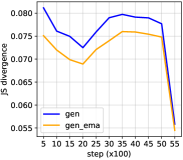
(b) TinyImageNet

(c) ImageNet

(d) Places365

Figure 4: Average Jensen-Shannon divergences between the prediction probabilities of $\mathtt{S}_{t-\tau}$ and $\mathtt{T}$ computed on synthetic samples from $\mathtt{G}_{t}$ (labeled as “gen”) and $\tilde{\mathtt{G}}_{t}$ (labeled as “gen_ema”) for different datasets. For CIFAR100 and TinyImageNet, we set $t\in[500,5500]$ with step size of 500 and $\tau=50$. For ImageNet and Places365, we set $t\in[100,1000]$ with step size of 100 and $\tau=10$. Note that the sudden drops at step 5000 in (a), (b) correspond to the decay of the learning rate by 0.1.

5.2.4 Visualization of synthetic samples

In Fig. 5, we visualize the synthetic data generated by $\mathtt{G}$ and $\tilde{\mathtt{G}}$. Although the generated images are not visually realistic, they are visually diverse, suggesting no mode collapse has occurred during training MAD. Besides, samples generated by $\tilde{\mathtt{G}}$ are different from those generated by $\mathtt{G}$ which indicates that the EMA generator could act as a complement for the generator in our model.

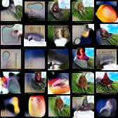
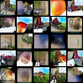
Generator	EMA Generator

(a) CIFAR100

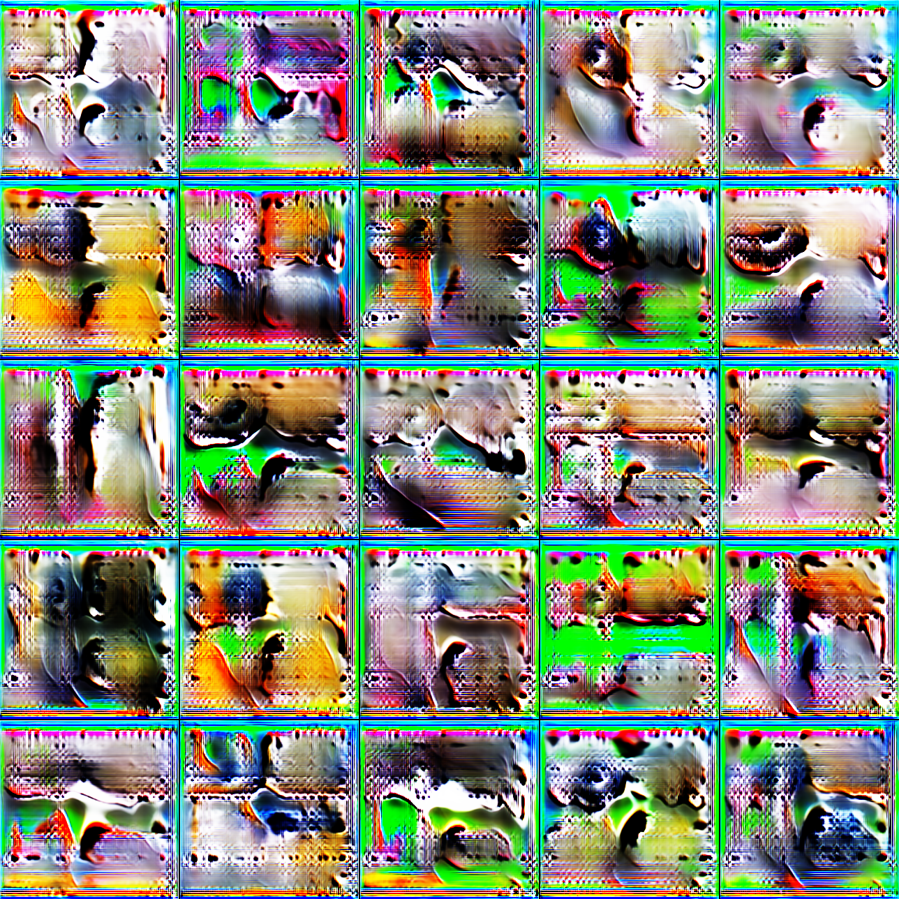
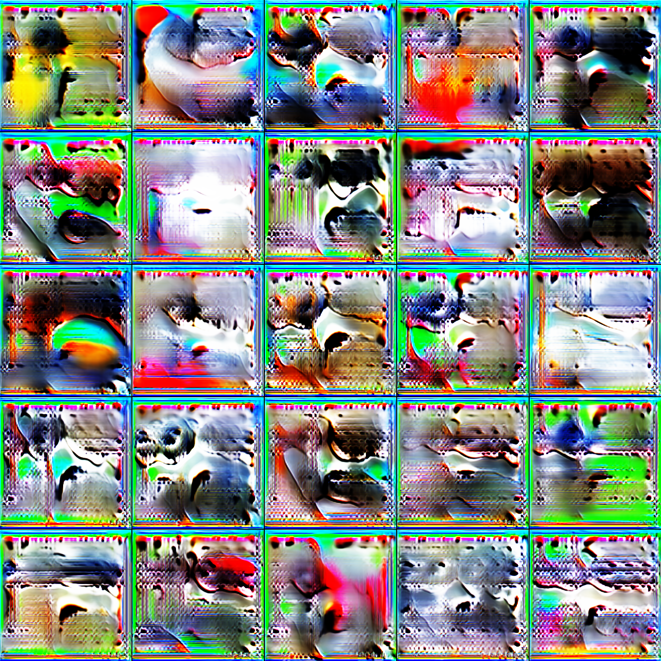
Generator	EMA Generator

(b) ImageNet

Figure 5: Synthetic data generated by $\mathtt{G}$ and $\tilde{\mathtt{G}}$ in case the original dataset is CIFAR100 (a) and ImageNet (b).

5.3 Sensitivity Analysis

Below we investigate some choices of hyperparameters that could affect the performance of MAD. Unless stated otherwise, the dataset we use is CIFAR100.

Different values of the coefficients in $\mathcal{L}_{\text{$\mathtt{S}$}}$

We can control the relative importance of samples from $\tilde{\mathtt{G}}$ over those from $\mathtt{G}$ by changing the values of the two coefficients $\lambda_{0}$ and $\lambda_{1}$ in $\mathcal{L}_{\mathtt{S}}$ (Eq. 4). As shown in Fig. 6 (right), the best result is obtained when $\lambda_{0}=\lambda_{1}=1$ which is our default setting for MAD. Decreasing either $\lambda_{0}$ or $\lambda_{1}$ will lead to worse performance. In the worst case when $\lambda_{0}=0$ and $\lambda_{1}=1$, the model learns for some epochs and then suddenly stops learning. The main reason is that $\tilde{\mathtt{G}}$ often updates much slower than $\mathtt{G}$ and $\mathtt{S}$ so we need adversarial samples from $\mathtt{G}$ to keep $\mathtt{S}$ learning. Otherwise, $\mathtt{S}$ will overfit the samples from $\tilde{\mathtt{G}}$ and learn nothing.

Different values of the momentum $\alpha$

In Fig. 6 (middle), we show the classification accuracy of the student of MAD with $\alpha$ in {0.2, 0.4, 0.6, 0.8, 0.95, 0.99, 0.999, 1.0}. We observe that the performance of our method increases when $\alpha$ becomes larger as $\tilde{\mathtt{G}}$ is more different from $\mathtt{G}$. However, if $\alpha$ is too large (e.g., 0.999), the performance drops since the update of $\mathtt{G}$ is very small, resulting in almost no change in the distribution of synthetic samples. In case $\alpha=1.0$, MAD only achieves about 50% prediction accuracy on test data.

		$\lambda_{0}$
		1.0	0.3	0.1	0.0
$\lambda_{1}$	1.0	64.05	63.26	62.43	1.08
	0.3	63.65	-	-	-
	0.1	62.80	-	-	-
	0.0	62.59	-	-	-

Figure 6: Test accuracy of our method w.r.t. different values of student update steps $n_{\mathtt{S}}$ (left), of the momentum $\alpha$ (middle), and of the coefficients ($\lambda_{0}$, $\lambda_{1}$) in Eq. 4 (right). The dataset is CIFAR100.

Different update steps of $\mathtt{S}$

From Fig. 6 (left), we see that increasing the number of update steps for $\mathtt{S}$ usually leads to better performances of MAD since $\mathtt{S}$ learns to match $\mathtt{T}$ better. In exchange, the training time will increase.

6 Conclusion

We have presented Momentum Adversarial Distillation (MAD), a simple yet effective method to deal with the large distribution shift problem in adversarial Data-Free Knowledge Distillation (DFKD). MAD maintains an exponential moving average (EMA) copy of the generator which, by design, encapsulates information about past updates of the generator and is updated at a slower pace than the generator. By training the student on samples from both the generator and the EMA generator, MAD can prevent the student from adapting too much to the generator at the current step and forgetting old knowledge learned from the generator at the previous steps. We have also described a new type of conditional generator along with a new loss for training it which enable our model to learn well on large datasets. Our experiments on various datasets demonstrated the superior performance of our method over competing baselines that either use only a generator or use a memory bank in place of an EMA generator.

We note that our idea of using an EMA generator to mitigate large distribution shifts is general and can be generalized to other machine learning problems besides DFKD. For example, the technique can be adapted for general continual learning (in which large distribution shifts can happen gradually or suddenly with no clear task boundaries), and source-data-free domain adaptation. Our method is also well suited for DFKD with other data types such as video, text, or graph.

Limitations

In our current implementation of MAD, we perform an additional forward pass through $\tilde{\mathtt{G}}$ for every training step of $\mathtt{S}$. This increases the total training time of by about 40% compared to ABM. However, this technical problem can be somewhat addressed by first storing synthetic samples from $\mathtt{G}$ and $\tilde{\mathtt{G}}$ in a buffer before each training stage of $\mathtt{S}$ and then training $\mathtt{S}$ with samples from the buffer only. This will be left for future work.

Negative Social Impacts

The DFKD problem may have negative social impacts related to data privacy as generated data could somehow reveal the original training data. However, as shown in Fig. 5, our proposed method does not attempt to improve the visual interpretability of synthetic data but addresses the large distribution shift problem. This target seems to be harmless to the society.

Acknowledgement

This research was partially funded by the Australian Government through the Australian Research Council (ARC). Prof. Venkatesh is the recipient of an ARC Australian Laureate Fellowship (FL170100006).

Appendix A Experimental Setup

A.1 Datasets

In Table 3, we provide information about the image size, the number of classes, and the number of training/test samples of the datasets used in our experiment.

Datatset	Image size	#classes	#train	#test
CIFAR10	$3\times 32\times 32$	10	50,000	10,000
CIFAR100		100	50,000	10,000
Tiny-ImageNet	$3\times 64\times 64$	200	100,000	10,000
ImageNet	$3\times 256\times 256$	1000	1,281,167	50,000
Places365		365	1,803,460	36,500
Food101		101	75,750	25,250

Table 3: Details of the datasets used in our experiment.

A.2 Training Settings of Teacher

We provide training settings of the teacher w.r.t. different datasets in Table 4.

Dataset	Training settings
	$opt$	$lr$	$wd$	$mo$	$bs$	$ls$	$ld$	$ldep$	$ep$	$wep$
CIFAR10/100	SGD	0.1	5e-4	0.9	128	No	0.1	80, 120	160	0
TinyImageNet					256	No
Food101		0.01	1e-4		512	Yes				5
Places365					1024	Yes		30, 60	90

Table 4: Training settings of teacher w.r.t. different datasets. Meanings of abbreviations: $opt$: optimizer, $lr$: learning rate, $wd$: weight decay, $mo$: momentum, $bs$: batch size, $ls$: scaling learning rate or not with the base batch size of 256 [15], $ld$: learning rate decay, $ldep$: epochs at which learning rate are decayed, $ep$: total number of epochs, $wep$: number of warm-up epochs.

A.3 Training Settings of MAD

In Tables A.3,A.3,7, we provide the training settings of MAD used in this paper. Despite multiple attempts, we could not find a global configuration that works well for all datasets and architectures.

In practice, we do not optimize the student and the generator via the plain losses in Eq. 4 and Eq. 6, respectively but with some additional regularizations on the output logits of $\mathtt{T}$, $\mathtt{S}$ and $\mathtt{G}$. This prevents our losses from being NaN when the logits grow too big. Specifically, we define $\mathcal{L}_{\mathtt{S}}$ as follows:

$$\mathcal{L}_{\mathtt{S}}\triangleq\ \lambda_{0}\mathbb{E}_{z\sim p(z),x=\mathtt{G}(z)}\left[\mathcal{L}_{\text{KD}}(x)+\zeta_{0}\max(\left|\mathtt{S}(x)\right|-\delta,0)\right]+$$

$$\lambda_{1}\mathbb{E}_{z^{\prime}\sim p(z),x^{\prime}=\tilde{\mathtt{G}}(z^{\prime})}\left[\mathcal{L}_{\text{KD}}(x^{\prime})+\zeta_{0}\max(\left|\mathtt{S}(x^{\prime})\right|-\delta,0)\right]$$ (10)

where $\max(\left|\mathtt{S}(\cdot)\right|-\delta,0)$ ensures that the output logit of $\mathtt{S}$ is between $[-\delta,\delta]$; $\zeta_{0}\geq 0$ is a coefficient.

And we define $\mathcal{L}_{\mathtt{G},\mathtt{E}}$ as follows:

$$\mathcal{L}_{\mathtt{G},\mathtt{E}}\triangleq\ \mathbb{E}_{z\sim\mathcal{N}(0,\mathrm{I}),y\sim\text{Cat}(C),u=\mathtt{G}_{\text{lg}}(z+y),x=\sigma(u)}\bigg{[}$$

$$\ \ \ \ \ \ \ \ \ \ \ \ \ \ \ \ \ \ \ -\lambda_{2}\mathcal{L}_{\text{KD}}(x)+\lambda_{3}\mathcal{L}_{\text{NLL}}(x,y)+\lambda_{4}\mathcal{L}_{\text{NormReg}}(e_{y})$$

$$\ \ \ \ \ \ \ \ \ \ \ \ \ \ \ \ \ \ \ +\zeta_{1}\max(|\mathtt{T}(x)|-\delta,0)+\zeta_{2}\max(|u|-\nu,0)\bigg{]}+\lambda_{5}\mathcal{L}_{\text{BNmm}}$$ (11)

where $\mathtt{G}_{\text{lg}}$ denotes the generator that produces logits instead of normalized images; $\sigma(\cdot)$ denotes the sigmoid function; $\max(|u|-\nu,0)$ ensures that the output logit $u$ of $\mathtt{G}_{\text{lg}}$ is between $[-\nu,\nu]$; $\max(|\mathtt{T}(x)|-\delta,0)$ ensures that the output logit of $\mathtt{T}$ w.r.t. the synthetic sample $x$ is between $[-\delta,\delta]$; $\zeta_{1},\zeta_{2}\geq 0$ are coefficients.

We train MAD on multiple NVIDIA A100-SXM2-32GB and A100-SXM4-40GB GPUs. Due to the use of different teacher/student architectures, the use of GPUs with different numbers and types, and the share of computational resources, it is hard to compute exactly the training time of our method but roughly it took about 1-2 days, 3-4 days, and 4-6 days to train MAD on CIFAR10/100, TinyImageNet, and ImageNet/Places365/Food101, respectively.

Dataset	Arch.	Student					Generator
		${opt}_{\mathtt{S}}$	${lr}_{\mathtt{S}}$	${wd}_{\mathtt{S}}$	${mo}_{\mathtt{S}}$	$n_{\mathtt{S}}$	${opt}_{\mathtt{G}}$	${lr}_{\mathtt{G}}$	${wd}_{\mathtt{G}}$	${mo}_{\mathtt{S}}$	$n_{\mathtt{G}}$
CIFAR10/100	$\heartsuit$	SGD	1e-2	5e-4	0.9	30	Adam	1e-3	5e-4	-	3
	$\diamondsuit$					60
TinyImageNet	$\heartsuit$					90
ImageNet	$\clubsuit$	Adam	1e-4	1e-4	-	150		1e-4			20
Places356											10
Food101											5

Table 5: Settings of optimizers for student and generator w.r.t. different datasets and architectures. The teacher/student architecture settings are ResNet34/ResNet18 ($\heartsuit$), WRN40-2/WRN16-2 ($\diamondsuit$), and AlexNet/AlexNet ($\clubsuit$). Meanings of abbreviations: $opt$: optimizer, $lr$: learning rate, $wd$: weight decay, $mo$: momentum, $n$: number of optimization steps.

Dataset	Training settings
	$bs$	$ld$	$ldep$	$ep$	$spe$	$d_{z}$	$\alpha$	$cg$	$\gamma$	$pg$	$pgs$	$\delta$	$\nu$
CIFAR10/100	256	0.1	100, 200	300	50	256	0.95	No	-	No	-	20	20
TinyImageNet									-
ImageNet	512	-	-	6000	1			Yes	1.1	Yes	200
Places365									1.1		50
Food101				4000					1.1

Table 6: Training settings of MAD w.r.t. different datasets. Meanings of abbreviations: $bs$: batch size, $ld$: learning rate decay, $ldep$: epochs at which learning rate are decayed, $ep$: total number of epochs, $spe$: steps per epoch, $d_{z}$: dimensionality of the noise $z$, $\alpha$: momentum for updating $\tilde{\mathtt{G}}$, $cg$: $\mathtt{G}$ is class-conditional or not, $\gamma$: the scaling hyperparameter in Eq. 8, $pg$: Pretraining $\mathtt{G}$ or not, $pgs$: Number of steps for pretraining $\mathtt{G}$, $\delta$: the bound in Eqs. 10,11, $\nu$: the bound in Eq. 11.

Dataset	Student			Generator
	$\lambda_{0}$	$\lambda_{1}$	$\zeta_{0}$	$\lambda_{2}$	$\lambda_{3}$	$\lambda_{4}$	$\lambda_{5}$	$\zeta_{1}$	$\zeta_{2}$
CIFAR10/100	1.0	1.0	0.01	1.0	0.0	0.0	1.0	0.1	0.1
TinyImageNet
ImageNet					0.1	0.1	0.0
Places365			0.1
Food101			0.1

Table 7: Coefficients of the loss terms in $\mathcal{L}_{\mathtt{S}}$ (Eq. 10) and $\mathcal{L}_{\mathtt{G}}$ (Eq. 11).

A.4 Generator Architectures

In Table 8, we show different architectures of the generator w.r.t. different image sizes.

Layer	Output size		Layer	Output size		Layer	Output size
Linear($d_{z}$, 4096)	4096		Linear($d_{z}$, 16384)	16384		Linear($d_{z}$, 8192)	8192
Reshape (16384, (256, 8, 8))	256$\times$4$\times$4		Reshape (16384, (256, 8, 8))	256$\times$8$\times$8		Reshape (8192, (512, 4, 4))	512$\times$4$\times$4
ReLU()	256$\times$4$\times$4		ReLU()	256$\times$8$\times$8		ResNetBlockY(512, 512)	512$\times$4$\times$4
BatchNorm2d(256, 0.1)	256$\times$4$\times$4		BatchNorm2d(256, 0.1)	256$\times$8$\times$8		UpsamplingBilinear2d(2)	512$\times$8$\times$8
UpsamplingBilinear2d(2)	256$\times$8$\times$8		UpsamplingBilinear2d(2)	256$\times$16$\times$16		ResNetBlockY(512, 256)	256$\times$8$\times$8
ConvBlockX(256, 128)	128$\times$8$\times$8		ConvBlockX(256, 128)	128$\times$16$\times$16		UpsamplingBilinear2d(2)	256$\times$16$\times$16
UpsamplingBilinear2d(2)	128$\times$16$\times$16		UpsamplingBilinear2d(2)	128$\times$32$\times$32		ResNetBlockY(256, 128)	128$\times$16$\times$16
ConvBlockX(128, 64)	64$\times$16$\times$16		ConvBlockX(128, 64)	64$\times$32$\times$32		UpsamplingBilinear2d(2)	128$\times$32$\times$32
UpsamplingBilinear2d(2)	64$\times$32$\times$32		UpsamplingBilinear2d(2)	64$\times$64$\times$64		ResNetBlockY(128, 64)	64$\times$32$\times$32
ConvBlockX(64, 32)	32$\times$32$\times$32		ConvBlockX(64, 32)	32$\times$64$\times$64		UpsamplingBilinear2d(2)	64$\times$64$\times$64
Conv2d(32, 3, 1, 0, 1)	3$\times$32$\times$32		Conv2d(32, 3, 1, 0, 1)	3$\times$64$\times$64		ResNetBlockY(64, 32)	32$\times$64$\times$64
						UpsamplingBilinear2d(2)	32$\times$128$\times$128
						ResNetBlockY(32, 16)	16$\times$128$\times$128
						UpsamplingBilinear2d(2)	16$\times$256$\times$256
						ResNetBlockY(16, 16)	16$\times$256$\times$256
						Conv2d(32, 3, 3, 1, 1)	3$\times$256$\times$256
(a) CIFAR10/CIFAR100			(b) TinyImageNet			(c) ImageNet/Places365/Food101

Table 8: Architectures of the generator w.r.t. different datasets. Details about ConvBlockX and ResNetBlockY are provided in Table 9.

ConvBlockX($c_{i}$, $c_{o}$)		ResNetBlockY($c_{i}$, $c_{o}$)
Conv2d($c_{i}$, $c_{o}$, 3, 1, 1)		Conv	Conv2d($c_{i}$, $c_{o}$, 3, 1, 1)
ReLU()			LeakyReLU(0.2)
BatchNorm2d($c_{o}$, 0.1)			BatchNorm2d($c_{i}$, 0.01)
Conv2d($c_{i}$, $c_{o}$, 3, 1, 1)			Conv2d($c_{o}$, $c_{o}$, 3, 1, 1)
ReLU()			LeakyReLU(0.2)
BatchNorm2d($c_{o}$, 0.1)			BatchNorm2d($c_{o}$, 0.01)
		Shortcut	$\begin{cases}\text{Conv2d($c_{i}$, $c_{o}$, 1, 0, 1)}&\text{if }c_{i}\neq c_{o}\\ \text{Identity()}&\text{otherwise}\end{cases}$
		Comp.	$y=\text{Conv}(x)+\text{Shortcut}(x)$
(a)		(b)

Table 9: Architectures of ConvBlockX (a) and ResNetBlockY (b).

Appendix B Additional Experimental Results

B.1 Results of Teacher

Table B.1 reports the results of our teacher on all the benchmark datasets. On the small datasets, our teacher achieves very similar performance compared to the one in [14].

	CIFAR10		CIFAR100		TinyIN	ImageNet	Places365	Food101
	ResNet34	WRN40-2	ResNet34	WRN40-2	ResNet34	AlexNet	AlexNet	AlexNet
Ours	95.46	94.65	78.55	75.65	66.47	56.52	50.80	65.15
In [14]	95.70	94.87	78.05	75.83	66.44	-	-	-

Table 10: Classification accuracies of our teacher and of the one in [14] on different datasets.

B.2 Results of DFKD-Mem with Different Memory Sizes

In Fig. 7, we show the classification results of DFKD-Mem with different memory sizes on CIFAR100 and ImageNet. On CIFAR100, DFKD-Mem achieves the best result at memory size = 2048 but still underperforms ABM and MAD. On ImageNet, the performance of DFKD-Mem is proportional to the memory size and is highest at memory size = 8192. This result, however, is still worse than that of MAD. Figs. 3a,3b display the average distillation loss (avg $\mathcal{L}_{\text{KD}}$) curves of DFKD-Mem w.r.t. different memory sizes. We see that increasing the memory size increases the avg $\mathcal{L}_{\text{KD}}$ on memory samples but does not affect the avg $\mathcal{L}_{\text{KD}}$ on samples from $\mathtt{G}$. It is because the avg $\mathcal{L}_{\text{KD}}$on memory samples is very small compared to the counterpart on samples from $\mathtt{G}$.

(a) CIFAR100

(b) ImageNet

Figure 7: Classification accuracies of DFKD-Mem with different memory sizes and of MAD, ABM on CIFAR100 and ImageNet.

(a) $\mathcal{L}_{\text{KD}}$ on memory samples

(b) $\mathcal{L}_{\text{KD}}$ on samples from $\mathtt{G}$

(c) $\mathcal{L}_{\text{KD}}$ on samples from $\tilde{\mathtt{G}}$

Figure 8: Distillation loss curves on memory samples (a) and samples generated by $\mathtt{G}$ (b) and $\tilde{\mathtt{G}}$ (c). The numbers in the legends denote DFKD-Mem with the corresponding memory sizes. “no_ema” and “ema” denote ABM and MAD, respectively. The dataset is ImageNet.

B.3 Empirical Analysis of Different Types of Generators

In Fig. B.3, we show the results of MAD on ImageNet with three different types of generators which are unconditional (“uncond”), conditional-via-concatenation (“cat”), conditional-via-summation (“sum”). MAD with the “uncond” generator eventually collapses during training but not with the “cat” or the “sum” generators (Fig. B.3a). This is because the “uncond” generator has learned to jump between different spurious solutions as visualized in Fig. B.3. Among all types of generators, the “sum” generator enables stable training of our model and gives the best accuracy and crossentropy on $\mathcal{D}_{\text{test}}$ (Figs. B.3a,b). The “cat” generator only yields good results at $\lambda_{3}=0.3$ ($\lambda_{3}$ is the coefficient of $\mathcal{L}_{\text{NLL}}$ in Eq. 6). The reason is that if $\lambda_{3}$ is too small (e.g., 0.1), $\mathcal{L}_{\text{NLL}}$ will be high (Fig. B.3g) and spurious solutions of $\mathtt{G}$ cannot be suppressed. $\mathtt{G}$ will jump between these solutions, leading to high variance when maximizing $\mathcal{L}_{\text{KD}}$ (Fig. B.3f). By contrast, if $\lambda_{3}$ is too big (e.g., 3.0, 10.0), $\mathtt{G}$ will be optimized towards predicting $y$ correctly (small $\mathcal{L}_{\text{NLL}}$ as shown in Fig. B.3g) rather than generating good adversarial samples for knowledge transfer from $\mathtt{T}$ to $\mathtt{S}$ (small $\mathcal{L}_{\text{KD}}$ as shown in Fig. B.3f). This causes $\mathtt{S}$ to achieve tiny $\mathcal{L}_{\text{KD}}$ (Fig. B.3e) and match $\mathtt{T}$ very well (Fig. B.3d) on samples from $\mathtt{G}$ but generalizes poorly to unseen sample from $\mathcal{D}_{\text{test}}$ (Fig. B.3a). However, for any value of $\lambda_{3}$, MAD with the “cat” generator performs worse than the counterpart with the “sum” generator, and even worse than the counterpart with the “uncond” generator during early epochs of training (Fig. B.3a). To explain this phenomenon, we first provide the formulas of the first layers of the three kinds of generators below as these generators are only different in the first layer:

uncond: $$h=Wz+b$$

cat: $$h=Wz+Ue_{y}+b$$

sum: $$h=Wz+We_{y}+b$$

where $W$, $U$, $b$ are trainable weights and bias. We hypothesize that due to the stochasticity of $z$ sampled from a fixed distribution, $W$ tends to be robust to changes. And since the “sum” generator uses $W$ to transform $e_{y}$, its output will not be affected much by the update of $e_{y}$. In other words, the noise in updating $e_{y}$ is absorbed into the stochasticity of $z$ via summation. The “cat” generator, on the other hand, uses a different weight matrix $U$ to transform $e_{y}$. Since the update of $U$ only depends on the current version of $e_{y}$ and vice versa, and $e_{y}$ can change arbitrarily, updating both $U$ and $e_{y}$ simultaneously in case of the “cat” generator can lead to unstable and nonoptimal training. The “uncond” generator does not encounter any problem with $e_{y}$ like the “cat” generator so it can enable MAD to learn faster than the “cat” generator.

(a) Test accuracy	(b) Test crossentropy	(c) Accuracy of $\mathtt{T}$	(d) $\mathtt{T}$-$\mathtt{S}$ match
(e) $\mathcal{L}_{\text{KD}}$ in training $\mathtt{S}$ (Eq. 4)	(f) $\mathcal{L}_{\text{KD}}$ in training $\mathtt{G}$ (Eq. 6)	(g) $\mathcal{L}_{\text{NLL}}$ in training $\mathtt{G}$ (Eq. 6)
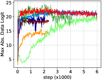
(h) $\max(|\mathtt{G}_{\text{lg}}|-20,0)$ (Eq. 11)	(i) Avg. of $\max|\mathtt{G}_{\text{lg}}|$ over pixels	(j) $\max(|\mathtt{T}(\mathtt{G})|-20,0)$ (Eq. 11)	(k) Avg. of $\max|\mathtt{T}(\mathtt{G})|$ over classes

Figure 9: Various learning curves of MAD with different types of generators: unconditional (“uncond”), conditional-via-summation (“sum”), and conditional-via-concatenation (“cat”). For the “uncond” generator, $e_{y}$ is set to non-trainable zero vector and $\lambda_{3}$, $\lambda_{4}$ in Eq. 6 are set to 0. For “cat” generators, the number behind “cat” in the legend indicates the coefficient of $\mathcal{L}_{\text{NLL}}$ ($\lambda_{3}$) in Eq. 6. We tried different coefficients and found that $\lambda_{3}=0.3$ works best for the “cat” generator. Except for Test accuracy and Test crossentropy which are computed on samples $\mathcal{D}_{\text{test}}$, all other quantities are computed on synthetic samples from $\mathtt{G}$.

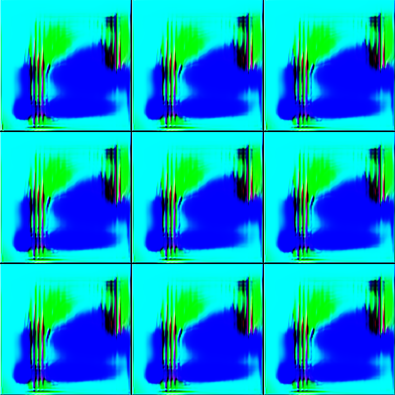
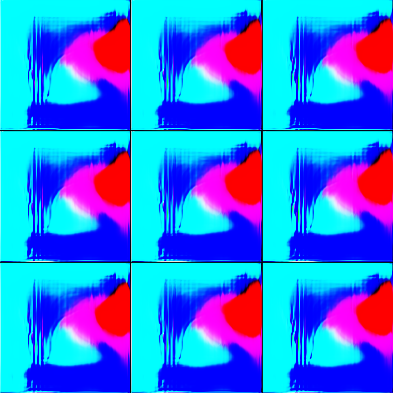
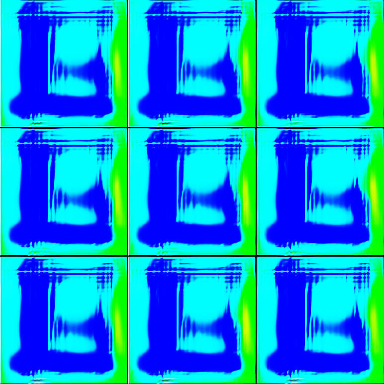
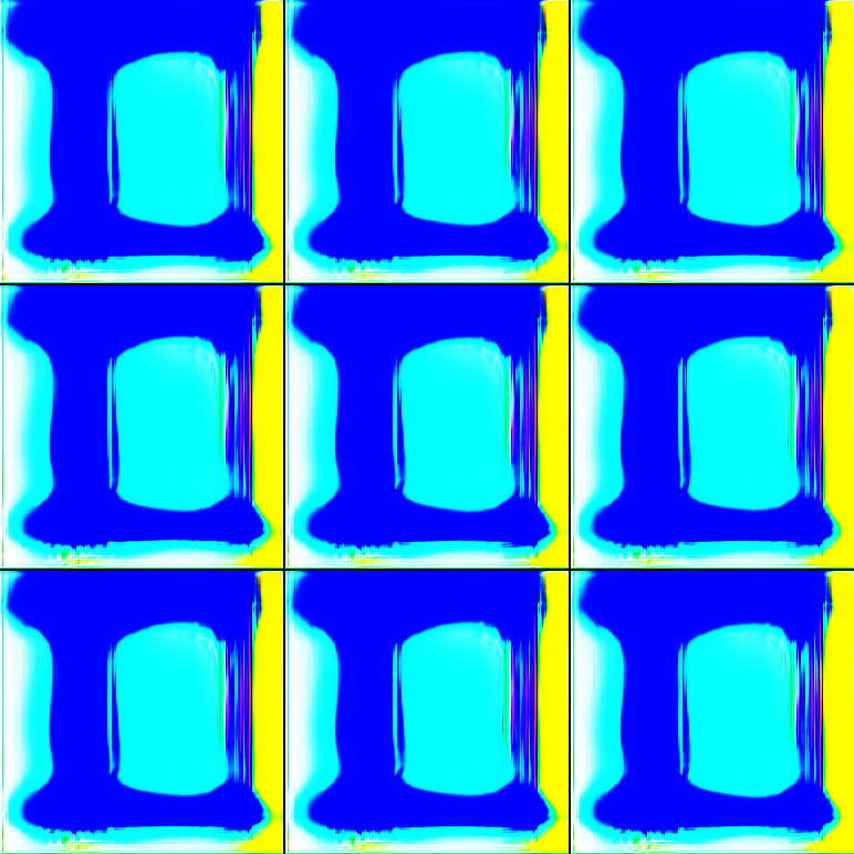
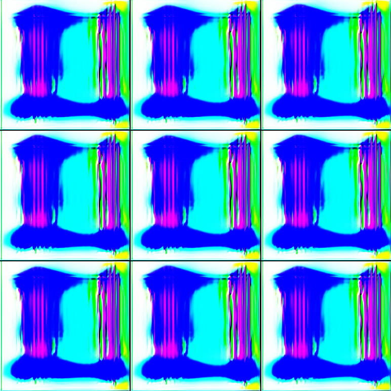
Train. Step	3900	3910	3920	3930	3940
Pred. Class	107	494	438	711	854
Confidence (%)	77.6	40.4	97.5	18.7	99.3

Figure 10: Visualization of generated samples from the unconditional generator whose has learning curves shown in Fig. B.3. It is obvious that this generator jumps between different spurious solutions during training, which results in the collapse of the student in Fig. B.3a.

Appendix C Derivation of $\mathcal{L}_{\text{NormReg}}$ in Section 3.2

Recall that in our design of the class-conditional generator, we use $K$ trainable class embedding vectors $e_{1},...,e_{K}$ to represent $K$ classes in the training data. These embedding vectors can be regarded as the centers of $K$ Gaussian distributions (or clusters) $\mathcal{N}(e_{k},\mathrm{I})$ ($k=1,...,K$) corresponding to $K$ classes and are optimized together with the generator $\mathtt{G}$ via Eq. 6. To prevent these embedding vectors from changing arbitrarily, we need to constraint their norms to be smaller than a threshold by minimizing the loss $\mathcal{L}_{\text{NormReg}}$ in Eq. 8. An important question is “What is a reasonable upper bound for the norm of each embedding vector $e_{k}$ ?”.

Let $\xi$ denote the upper bound for the norm of $e_{k}$. By constraining $\left\|e_{k}\right\|_{2}$ to be smaller than $\xi$, we ensure that $e_{k}$ is inside a hyperball of radius $\xi$. Intuitively, we should choose $\xi$ so that the $K$ Gaussian clusters won’t overlap each other. Note that in high dimensional space, we can generally treat each Gaussian cluster $\mathcal{N}(e_{k},\mathrm{I})$ as a hypersphere of radius $\sqrt{d_{e}}$ centered at $e_{k}$ ($d_{e}=\dim(e_{k})$). One simple way to allow these $K$ hyperspheres not to overlap each other when their centers are inside a hyperball of radius $\xi$ is to make sure that the total volume of $K$ hyperballs of radius $\sqrt{d_{e}}$ is smaller than the volume of the hyperball of radius $\xi$. Mathematically, it means:

$$K\times\mathcal{V}_{d_{e}}\left(\sqrt{d_{e}}\right)<\mathcal{V}_{d_{e}}\left(\xi\right)$$

$$\Leftrightarrow K\times\left(\sqrt{d_{e}}\right)^{d_{e}}\times\mathcal{V}_{d_{e}}\left(1\right)<\xi^{d_{e}}\times\mathcal{V}_{d_{e}}\left(1\right)$$

$$\Leftrightarrow K^{1/d_{e}}\sqrt{d_{e}}<\xi$$

where $\mathcal{V}_{d}(r)$ denotes the volume of a $d$-ball of radius $r$. When $d_{e}$ is large, $K^{1/d_{e}}\approx 1$ and can be ignored. Thus, we should choose $\xi$ to have the form $\gamma\times\sqrt{d_{e}}$ with $\gamma\geq 1$.

References

- [1] Sungsoo Ahn, Shell Xu Hu, Andreas Damianou, Neil D Lawrence, and Zhenwen Dai. Variational information distillation for knowledge transfer. In Proceedings of the IEEE/CVF Conference on Computer Vision and Pattern Recognition, pages 9163–9171, 2019.
- [2] Kuluhan Binici, Shivam Aggarwal, Nam Trung Pham, Karianto Leman, and Tulika Mitra. Robust and resource-efficient data-free knowledge distillation by generative pseudo replay. arXiv preprint arXiv:2201.03019, 2022.
- [3] Kuluhan Binici, Nam Trung Pham, Tulika Mitra, and Karianto Leman. Preventing catastrophic forgetting and distribution mismatch in knowledge distillation via synthetic data. In Proceedings of the IEEE/CVF Winter Conference on Applications of Computer Vision, pages 663–671, 2022.
- [4] Lukas Bossard, Matthieu Guillaumin, and Luc Van Gool. Food-101 - mining discriminative components with random forests. In European Conference on Computer Vision, 2014.
- [5] Nicolas Carion, Francisco Massa, Gabriel Synnaeve, Nicolas Usunier, Alexander Kirillov, and Sergey Zagoruyko. End-to-end object detection with transformers. In European conference on computer vision, pages 213–229. Springer, 2020.
- [6] Akshay Chawla, Hongxu Yin, Pavlo Molchanov, and Jose Alvarez. Data-free knowledge distillation for object detection. In Proceedings of the IEEE/CVF Winter Conference on Applications of Computer Vision, pages 3289–3298, 2021.
- [7] Hanting Chen, Yunhe Wang, Chang Xu, Zhaohui Yang, Chuanjian Liu, Boxin Shi, Chunjing Xu, Chao Xu, and Qi Tian. Data-free learning of student networks. In Proceedings of the IEEE/CVF International Conference on Computer Vision, pages 3514–3522, 2019.
- [8] Yoojin Choi, Jihwan Choi, Mostafa El-Khamy, and Jungwon Lee. Data-free network quantization with adversarial knowledge distillation. In Proceedings of the IEEE/CVF Conference on Computer Vision and Pattern Recognition Workshops, pages 710–711, 2020.
- [9] Jia Deng, Wei Dong, Richard Socher, Li-Jia Li, Kai Li, and Li Fei-Fei. Imagenet: A large-scale hierarchical image database. In 2009 IEEE Conference on Computer Vision and Pattern Recognition, pages 248–255. IEEE, 2009.
- [10] Jacob Devlin, Ming-Wei Chang, Kenton Lee, and Kristina Toutanova. Bert: Pre-training of deep bidirectional transformers for language understanding. arXiv preprint arXiv:1810.04805, 2018.
- [11] Gongfan Fang, Yifan Bao, Jie Song, Xinchao Wang, Donglin Xie, Chengchao Shen, and Mingli Song. Mosaicking to distill: Knowledge distillation from out-of-domain data. Advances in Neural Information Processing Systems, 34:11920–11932, 2021.
- [12] Gongfan Fang, Kanya Mo, Xinchao Wang, Jie Song, Shitao Bei, Haofei Zhang, and Mingli Song. Up to 100x faster data-free knowledge distillation. arXiv preprint arXiv:2112.06253, 2021.
- [13] Gongfan Fang, Jie Song, Chengchao Shen, Xinchao Wang, Da Chen, and Mingli Song. Data-free adversarial distillation. arXiv preprint arXiv:1912.11006, 2019.
- [14] Gongfan Fang, Jie Song, Xinchao Wang, Chengchao Shen, Xingen Wang, and Mingli Song. Contrastive model inversion for data-free knowledge distillation. arXiv preprint arXiv:2105.08584, 2021.
- [15] Priya Goyal, Piotr Dollár, Ross Girshick, Pieter Noordhuis, Lukasz Wesolowski, Aapo Kyrola, Andrew Tulloch, Yangqing Jia, and Kaiming He. Accurate, large minibatch sgd: Training imagenet in 1 hour. arXiv preprint arXiv:1706.02677, 2017.
- [16] Ishaan Gulrajani, Faruk Ahmed, Martin Arjovsky, Vincent Dumoulin, and Aaron C Courville. Improved training of wasserstein gans. Advances in neural information processing systems, 30, 2017.
- [17] Pengchao Han, Jihong Park, Shiqiang Wang, and Yejun Liu. Robustness and diversity seeking data-free knowledge distillation. In ICASSP 2021-2021 IEEE International Conference on Acoustics, Speech and Signal Processing (ICASSP), pages 2740–2744. IEEE, 2021.
- [18] Kaiming He, Xiangyu Zhang, Shaoqing Ren, and Jian Sun. Deep residual learning for image recognition. In Proceedings of the IEEE conference on computer vision and pattern recognition, pages 770–778, 2016.
- [19] Geoffrey Hinton, Oriol Vinyals, and Jeff Dean. Distilling the knowledge in a neural network. arXiv preprint arXiv:1503.02531, 2015.
- [20] Sergey Ioffe and Christian Szegedy. Batch normalization: Accelerating deep network training by reducing internal covariate shift. In International conference on machine learning, pages 448–456. PMLR, 2015.
- [21] Diederik P Kingma and Jimmy Ba. Adam: A Method for Stochastic Optimization. arXiv preprint arXiv:1412.6980, 2014.
- [22] Diederik P Kingma and Max Welling. Auto-encoding variational bayes. arXiv preprint arXiv:1312.6114, 2013.
- [23] James Kirkpatrick, Razvan Pascanu, Neil Rabinowitz, Joel Veness, Guillaume Desjardins, Andrei A Rusu, Kieran Milan, John Quan, Tiago Ramalho, Agnieszka Grabska-Barwinska, et al. Overcoming catastrophic forgetting in neural networks. Proceedings of the national academy of sciences, 114(13):3521–3526, 2017.
- [24] Alex Krizhevsky. Learning multiple layers of features from tiny images. Technical report, 2009.
- [25] Ya Le and Xuan Yang. Tiny imagenet visual recognition challenge. Technical report, 2015.
- [26] Kevin J Liang, Chunyuan Li, Guoyin Wang, and Lawrence Carin. Generative adversarial network training is a continual learning problem. arXiv preprint arXiv:1811.11083, 2018.
- [27] Raphael Gontijo Lopes, Stefano Fenu, and Thad Starner. Data-free knowledge distillation for deep neural networks. arXiv preprint arXiv:1710.07535, 2017.
- [28] James Lucas, George Tucker, Roger Grosse, and Mohammad Norouzi. Understanding posterior collapse in generative latent variable models. 2019.
- [29] Liangchen Luo, Mark Sandler, Zi Lin, Andrey Zhmoginov, and Andrew Howard. Large-scale generative data-free distillation. arXiv preprint arXiv:2012.05578, 2020.
- [30] Qi Mao, Hsin-Ying Lee, Hung-Yu Tseng, Siwei Ma, and Ming-Hsuan Yang. Mode seeking generative adversarial networks for diverse image synthesis. In Proceedings of the IEEE/CVF conference on computer vision and pattern recognition, pages 1429–1437, 2019.
- [31] Paul Micaelli and Amos J Storkey. Zero-shot knowledge transfer via adversarial belief matching. Advances in Neural Information Processing Systems, 32, 2019.
- [32] Alexander Mordvintsev, Christopher Olah, and Mike Tyka. Inceptionism: Going deeper into neural networks. 2015.
- [33] Gaurav Kumar Nayak, Konda Reddy Mopuri, and Anirban Chakraborty. Effectiveness of arbitrary transfer sets for data-free knowledge distillation. In Proceedings of the IEEE/CVF Winter Conference on Applications of Computer Vision, pages 1430–1438, 2021.
- [34] Gaurav Kumar Nayak, Konda Reddy Mopuri, Vaisakh Shaj, Venkatesh Babu Radhakrishnan, and Anirban Chakraborty. Zero-shot knowledge distillation in deep networks. In International Conference on Machine Learning, pages 4743–4751. PMLR, 2019.
- [35] Wonpyo Park, Dongju Kim, Yan Lu, and Minsu Cho. Relational knowledge distillation. In Proceedings of the IEEE/CVF Conference on Computer Vision and Pattern Recognition, pages 3967–3976, 2019.
- [36] Nikolaos Passalis and Anastasios Tefas. Learning deep representations with probabilistic knowledge transfer. In Proceedings of the European Conference on Computer Vision (ECCV), pages 268–284, 2018.
- [37] Xiaoyang Qu, Jianzong Wang, and Jing Xiao. Enhancing data-free adversarial distillation with activation regularization and virtual interpolation. In ICASSP 2021-2021 IEEE International Conference on Acoustics, Speech and Signal Processing (ICASSP), pages 3340–3344. IEEE, 2021.
- [38] Alec Radford, Jong Wook Kim, Chris Hallacy, Aditya Ramesh, Gabriel Goh, Sandhini Agarwal, Girish Sastry, Amanda Askell, Pamela Mishkin, Jack Clark, et al. Learning transferable visual models from natural language supervision. In International Conference on Machine Learning, pages 8748–8763. PMLR, 2021.
- [39] James Smith, Yen-Chang Hsu, Jonathan Balloch, Yilin Shen, Hongxia Jin, and Zsolt Kira. Always be dreaming: A new approach for data-free class-incremental learning. In Proceedings of the IEEE/CVF International Conference on Computer Vision, pages 9374–9384, 2021.
- [40] Hoang Thanh-Tung and Truyen Tran. Catastrophic forgetting and mode collapse in gans. In 2020 International Joint Conference on Neural Networks (IJCNN), pages 1–10. IEEE, 2020.
- [41] Yonglong Tian, Dilip Krishnan, and Phillip Isola. Contrastive representation distillation. In International Conference on Learning Representations, 2019.
- [42] Frederick Tung and Greg Mori. Similarity-preserving knowledge distillation. In Proceedings of the IEEE/CVF International Conference on Computer Vision, pages 1365–1374, 2019.
- [43] Ashish Vaswani, Noam Shazeer, Niki Parmar, Jakob Uszkoreit, Llion Jones, Aidan N Gomez, Łukasz Kaiser, and Illia Polosukhin. Attention is all you need. Advances in neural information processing systems, 30, 2017.
- [44] Zi Wang. Data-free knowledge distillation with soft targeted transfer set synthesis. In Proceedings of the AAAI Conference on Artificial Intelligence, volume 35, pages 10245–10253, 2021.
- [45] Hongxu Yin, Pavlo Molchanov, Jose M Alvarez, Zhizhong Li, Arun Mallya, Derek Hoiem, Niraj K Jha, and Jan Kautz. Dreaming to distill: Data-free knowledge transfer via deepinversion. In Proceedings of the IEEE/CVF Conference on Computer Vision and Pattern Recognition, pages 8715–8724, 2020.
- [46] Jaemin Yoo, Minyong Cho, Taebum Kim, and U Kang. Knowledge extraction with no observable data. Advances in Neural Information Processing Systems, 32, 2019.
- [47] Sergey Zagoruyko and Nikos Komodakis. Paying more attention to attention: Improving the performance of convolutional neural networks via attention transfer. arXiv preprint arXiv:1612.03928, 2016.
- [48] Sergey Zagoruyko and Nikos Komodakis. Wide residual networks. In British Machine Vision Conference 2016. British Machine Vision Association, 2016.
- [49] Friedemann Zenke, Ben Poole, and Surya Ganguli. Continual learning through synaptic intelligence. In International Conference on Machine Learning, pages 3987–3995. PMLR, 2017.
- [50] Haoran Zhao, Xin Sun, Junyu Dong, Milos Manic, Huiyu Zhou, and Hui Yu. Dual discriminator adversarial distillation for data-free model compression. International Journal of Machine Learning and Cybernetics, pages 1–18, 2021.
- [51] Bolei Zhou, Agata Lapedriza, Aditya Khosla, Aude Oliva, and Antonio Torralba. Places: A 10 million image database for scene recognition. IEEE Transactions on Pattern Analysis and Machine Intelligence, 2017.