Schema-Based Automata Determinization

Abstract

We propose an algorithm for schema-based determinization of finite automata on words and of stepwise hedge automata on nested words. The idea is to integrate schema-based cleaning directly into automata determinization. We prove the correctness of our new algorithm and show that it is always more efficient than standard determinization followed by schema-based cleaning. Our implementation permits to obtain a small deterministic automaton for an example of an XPath query, where standard determinization yields a huge stepwise hedge automaton for which schema-based cleaning runs out of memory.

1 Introduction

Nested words are words enhanced with well-nested parenthesis. They generalize over trees, unranked trees, and sequences of thereof that are also called hedges or forests. Nested words provide a formal way to represent semi-structured textual documents of XML and JSON format.

Regular queries for nested words can be defined by finite state automata. We will use stepwise hedge automata (Shas) for this purpose [Sakho], which combine finite state automata for words and trees in a natural manner. Shas refine previous notions of hedge automata from the sixties [Thatcher67b, TATA07] in order to obtain a decent notion of left-to-right and bottom-up determinism. They extend on stepwise tree automata [CarmeNiehrenTommasi04], so that they can not only be applied to unranked trees but also to hedges. Any Sha defines a forest algebra [DBLP:conf/birthday/BojanczykW08] based on its transition relation. Furthermore, Shas can always be determinized and have the same expressiveness as (deterministic) nested word automaton (Nwa) [DBLP:conf/icalp/Mehlhorn80, BRAUNMUHL19851, Alur07, DBLP:journals/sigact/OkhotinS14]. Note, however, that Shas do not provide any form of top-down determinism in contrast to $\textsc{Nwa}s$.

Efficient compilers from regular XPath queries to Shas exist [Sakho], possibly using $\textsc{Nwa}s$ as intermediates [AlurMadhusudan09, MozafariZengZaniolo12, debarbieux15]. Our main motivation is to determinize the Shas of regular XPath queries since deterministic automata are crucial for various algorithmic querying tasks. In particular, determinism reduce the complexity of universality or inclusion checking from EXP-completeness to P-time, both for the classes of deterministic Shas or $\textsc{Nwa}s$. In turn, universality checking is relevant for the earliest query answering of XPath queries on XML streams [GauwinNiehrenTison09b]. Furthermore, determinism is needed for efficient in-memory answer enumeration of regular queries [schmid_et_al:LIPIcs.ICDT.2021.4].

Automata determinization may take exponential time in the worst case, so it may not always be feasible in practice. For Shas compiled from the XPath queries of the XPathMark benchmark [FranceschetXPathPT], however, it was shown to be unproblematic. This changes for the XPath benchmark collected by Lick and Schmitz [lickbench]: for 37% of its regular XPath queries, Sha determinization does require more than 100 seconds, in which case it produces huge deterministic automata [alserhalibench]. An example is:

      (QN7)     /a/b//(* | @* | comment() | text())

This XPath query selects all nodes of an XML document that are descendants of a $b$-element below an $a$-element at the root. The nodes may have any XML type: element, attribute, comment, or text. The nondeterministic Sha for QN7 has $145$ states and an overall size of $348$. Its determinization however leads to an automaton with $10.005$ states and an overall size of $1.634.122$.

A kick-off question is how to reduce the size of deterministic automata. One approach beside of minimization is to apply schema-based cleaning [Sakho], where the schema of a query defines to which nested words the query can be applied. Schemas are always given by deterministic automata while the automata for queries may be nondeterministic. The idea of schema-based automaton cleaning is to keep only those states and transition rules of the automaton, that are needed to recognize some nested word satisfying the schema. The needed states and rules can be found by building the product of automata for the query and the schema. For XPath queries selecting nodes, we have the schema ${{one^{x}}}$ that states that a single node is selected for a fixed variable $x$ by any answer of the query. The second schema expresses which nested words satisfy the XML data model. With the intersection of these two schemas, the schema-based cleaning of the deterministic Sha for QN7 indeed has only $74$ states and $203$ rules. When applying Sha minimization afterwards, the size of the automaton goes down to $27$ states and $71$ transition rules. However, our implementation of schema-based cleaning, runs out of memory for larger automata with say more than $1000$ states. Therefore, we cannot compute the schema-based cleaning from the deterministic Sha obtained from QN7. Neither can we minimize it with our implementation of deterministic Sha minimization. The question of how to produce small deterministic automaton for queries as simple as QN7 thus needs a different answer.

Given the relevance of schemas, one naive approach could be to determinize the product of the automata for the query and schema. This may look questionable at first sight, given that the schema-product may be bigger than the original automaton, so why could it make determinization more efficient? But in the case of QN7, the determinization of the schema-product yields a deterministic automata with only $92$ states and $325$ transition rules, and can be computed efficiently. This observation is very promising, motivating three general questions:

1. Why are schemas so important for automata determinization?

2. Can this be established by some complexity result?

3. Is there a way to compute the schema-based cleaning of the determinization of an Sha more efficiently than be schema-based cleaning followed by determinization?

Our main result is a novel algorithm for schema-based determinization of Nfas and Shas, that integrates schema-based cleaning directly into the usual determinization algorithm. This algorithm answers question 3 positively. Its idea is to keep only those subsets of states of the automaton during the determinization, that can be aligned to some state of the schema. In our Theorem 23, we prove that schema-based determinization always produces the same deterministic automaton than schema-free determinization followed by schema-based cleaning. By schema-based determinization we could compute the schema-based cleaning of the determinization of QN7 in less than three seconds. In contrast, the schema-based cleaning of the determinization does not terminate after a few hours. In the general case, the worst case complexity of schema-based determinization is lower than schema-less determinization followed by schema-based cleaning.

We also provide a more precise complexity upper bound in Proposition 7. Given an nondeterministic Sha $A$ let $det(A)$ be its determinization, and given a deterministic Sha $S$ for the schema, let $A\times S$ the accessible part of the schema-product, and $\mathit{scl}_{S}(A)$ the schema-based cleaning of $S$ with respect to schema $S$. We show that the upper bound for the maximal computation time of $\mathit{scl}_{S}(det(A))$ depends quadratically on the number of states of $S\times det(A)$, which is often way smaller than for $det(A)$ since $S$ is deterministic. This complexity result shows why the schema is so relevant for determinization (questions 1 and 2), and why computing the schema-based determinization is often more efficient than determinization followed by schema-based cleaning (question 3).

To see that $S\times det(A)$ is often way smaller than $det(A)$ for deterministic $S$ we first note that $det(A\times S)=det(A)\times S$ since $S$ is deterministic. So for the many states $Q=\{q_{1}\ldots q_{n}\}$ of $det(A)$ there may not exist any state $s$ of $S$ such that $(Q,s)\in det(A)\times S$, because this requires all states $q_{i}$ can be aligned to $s$, i.e. that $(q_{i},s)$ in $A\times S$ for all $1\leq i\leq n$. Furthermore, $\det(A)\times S$ is equal to $\mathit{det}_{S}(A)\times S$, so that $det(A\times S)=\mathit{det}_{S}(A)\times S$. Hence any size bound for the schema-based determinization $\mathit{det}_{S}(A)$ implies a size bound for the determinization of the schema-product. Also, in our experiments $\mathit{det}_{S}(A)\times S$ is almost by a factor of $2$ bigger than $\mathit{det}_{S}(A)$. So the size of the determinization of the schema-product is closely tied to the size of the schema-based determinization.

We also present a experimental evaluation of our implementation of schema-based determinization of Shas. We consider a scalable family of Shas obtained from a scalable family of XPath queries. Our experiments confirm the very large improvement implied by the usage of schemas for determinization. For this, we implemented the algorithm for schema-based Sha determinization in Scala. Furthermore, we applied the XSLT compiler from regular forward XPath queries to Shas from [Sakho], as well as the datalog implementations of Sha minimization and schema-based cleaning from there.

A large scale experiment on practical XPath queries was provided in follow-up work [alserhalibench] where schema-based algorithms were applied to the regular XPath queries collected by Lick and Schmitz [lickbench] from real word XQuery and XSLT programs. Small deterministic Shas could be obtained by schema-based determinization for all regular XPath queries in this corpus. In contrast, standard determinization in 37% of the cases fails with a timeout of 100 seconds. Without this timeout, determinization either runs out of memory or produces very large automata.

Outline

We start with related work on automata for nested words, determinization for XPath queries (Section 2). In Section 3, we recall the definition Nfas and discuss how to use them as schemas and queries on words. In Section 4, we recall schema-based cleaning for Nfas. In Section 5, we contribute our schema-based determinization algorithm in the case of Nfas and show its correctness. In Section 6, we recall the notion of Shas for defining languages of nested words. In Section 7, we lift schema-based determinization to Shas. Full proofs can be found in the Appendix of the long version [niehrenschemadet].

2 Related Work

We focus on automata for nested words, even though our results are new for Nfas too.

Nested word automata

As recalled in the survey of Okhotin and Salomaa [DBLP:journals/sigact/OkhotinS14], Alur’s et al. [Alur07] $\textsc{Nwa}s$ were first introduced in the eighties under the name of input driven automata by Mehlhorn [DBLP:conf/icalp/Mehlhorn80], and then reinvented several times under different names. In particular, they were called visibly pushdown automata [AlurMadhusudan04], pushdown forest automata [NeumannSeidl98], and streaming tree automata [GauwinNiehrenRoos08]. The determinization algorithm for $\textsc{Nwa}s$ was first invented in the eighties by von Braunmühl and Verbeek in the journal version of [BRAUNMUHL19851] and then rediscovered various times later on too.

Determinization algorithms

The usual determinization algorithms for Nfas relies on the well-known subset construction. The determinization algorithms of bottom-up tree automata and Shas are straightforward extensions thereof. The determinization algorithm for $\textsc{Nwa}s$, in contrast, is more complicated, since having to deal with pushdowns. Subsets of pairs of states are to be considered there and not only subsets of states as with the usual automata determinization algorithm. We also notice that general pushdown automata with nonvisible stacks can even not always be determinized.

Application to XPath

Debarbieux et al. [debarbieux15] noticed that the determinization algorithm for $\textsc{Nwa}s$ often behaves badly when applied to $\textsc{Nwa}s$ obtained from XPath queries as simple as $//a/b$. Niehren and Sakho [Sakho] observed more recently that the situation is different for the determinization of Shas: It works out nicely for the Sha of $//a/b$ and also for all other Shas obtained by compilation from forward navigational XPath queries in the XPathMark benchmark [FranceschetXPathPT]. Even more surprisingly, the same good behavior could be observed for the determinization algorithm of Nwa when restricted to $\textsc{Nwa}s$ with the weak-single entry property.

Weak single-entry $\textsc{Nwa}s$ versus Shas

The weak-single entry property implies that an Nfa cannot memoize anything in its state when moving top-down. So it can only pass information left-to-right and and bottom-up, similarly to an Sha. This property failed for the $\textsc{Nwa}s$ considered by Debarbieux et al. and the determinization of their $\textsc{Nwa}s$ thus required top-down determinization. This quickly led to the size explosion described above. One the other hand side, the weak single-entry property can always be established in quadratic time by compiling $\textsc{Nwa}s$ to Shas forth and back. Or else, one can avoid top-down determinization all over by directly working with Shas as we do here.

3 Finite Automata on Words, Schemas, and Queries

In this section, we discuss hwo to use Nfas for defining schemas and queries on words.

Let $\mathbb{N}$ be the set of natural numbers including $0$. The set of words over a finite alphabet $\Sigma$ is $\Sigma^{*}=\bigcup\limits_{n\in\mathbb{N}}^{\infty}\Sigma^{n}$. A word $(a_{1},\ldots,a_{n})\in\Sigma^{n}$ is written as $a_{1}\ldots a_{n}$. We denote by $\varepsilon$ the empty word, i.e., the unique element of $\Sigma^{0}$ and by $w_{1}\cdot w_{2}\in\Sigma^{*}$ the concatenation of two words $w_{1},w_{2}\in\Sigma^{*}$. For example, if $\Sigma=\{a,b\}$ then $aa\cdot bb=aabb=a\cdot a\cdot b\cdot b$.

Definition 3.1.

A Nfa is a tuple $A=(\Sigma,\mathcal{Q},\Delta,I,F)$ such that $\mathcal{Q}$ is a finite set of states, the alphabet $\Sigma$ is a finite set, $I,F\subseteq\mathcal{Q}$ are subsets of initial and final states, and $\Delta\subseteq\mathcal{Q}\times\Sigma\times\mathcal{Q}$ is the set of transition rules.

The size of a Nfa is $|A|=|\mathcal{Q}|+|\Delta|$. A transition rule $(q,a,q^{\prime})\in\Delta$ is denoted by $q\xrightarrow{a}q^{\prime}\in\Delta$. We define transitions $q\xrightarrow{w}q^{\prime}\text{ wrt }\Delta$ for arbitrary words $w\in\Sigma^{*}$ by the following inference rules:

$$q\xrightarrow{\varepsilon}q\text{ wrt }\Delta q\in\mathcal{Q}\qquad q\xrightarrow{a}q^{\prime}\text{ wrt }\Delta q\xrightarrow{a}q^{\prime}\in\Delta\qquad q_{0}\xrightarrow{w_{1}\cdot w_{2}}q_{2}\text{ wrt }\Delta q_{0}\xrightarrow{w_{1}}q_{1}\text{ wrt }\Delta\qquad q_{1}\xrightarrow{w_{2}}q_{2}\text{ wrt }\Delta$$

The language of words recognized by a Nfa then is $\mathcal{L}(A)=\{w\in\Sigma^{*}\mid q\xrightarrow{w}q^{\prime}\text{ wrt }\Delta,\ q\in I,\ q^{\prime}\in F\}$.

$$I^{A}\in I^{det(A)}\qquad I^{A}\in\mathcal{Q}^{\det(A)}I^{A}\not=\emptyset\qquad Q\in\mathit{F}^{\det(A)}Q\in\mathcal{Q}^{\det(A)}\quad Q\cap\mathit{F}^{A}\not=\emptyset$$

$$Q\xrightarrow{a}Q^{\prime}\in\Delta^{det(A)}\qquad Q^{\prime}\in\mathcal{Q}^{\det(A)}\begin{array}[]{c}Q\in\mathcal{Q}^{\det(A)}\qquad Q^{\prime}=\{q^{\prime}\in\mathcal{Q}^{A}\mid q\xrightarrow{a}q^{\prime}\in\Delta^{A},\ q\in Q\}\not=\emptyset\end{array}$$

$$\det(A)=(\Sigma,\mathcal{Q}^{\det(A)},\Delta^{\det(A)},I^{\det(A)},F^{\det(A)})$$

Figure 1: The accessible determinization $\det(A)$ of Nfa $A$.

⬇

1fun det($A$) =

2 let $Store=hashset.new(\emptyset)$ and $Agenda=list.new()$ and $Rules=hashset.new(\emptyset)$

3 if $\mathit{init}^{A}\not=\emptyset$ then $Agenda.add(\mathit{init}^{A})$

4 while $Agenda.notEmpty()$ do

5 let $Q=Agenda.pop()$

6 let $h$ be an empty hash table with keys from $\Sigma$.

7 // the values will be nonempty hash subsets of $\mathcal{Q}^{A}$

8 for $q\xrightarrow{a}q^{\prime}\in\Delta^{A}$ such that $q\in Q$ do

9 if $h.get(a)=undef$ then $h.add(a,hashset.new(\emptyset))$

10 $(h.get(a)).add(q^{\prime})$

11 for $(a,Q^{\prime})$ in $h.tolist()$ do $Rules.add(Q\xrightarrow{a}Q^{\prime})$

12 if not $Store.member(Q^{\prime})$ then $Store.add(Q^{\prime})$ $Agenda.push(Q^{\prime})$

13 let $\mathit{init}^{det(A)}=\{Q\mid Q\in Store,Q\cap\mathit{init}^{A}\not=\emptyset\}$ and $F^{det(A)}=\{Q\mid Q\in Store,Q\cap F^{A}\not=\emptyset\}$

14 return $(\Sigma,Store.toSet(),Rules.toSet(),\mathit{init}^{det(A)},F^{det(A)})$

Figure 2: A program computing the accessible determinization of an Nfa $A$ from Figure 1.

A Nfa $A$ is called deterministic or equivalently a Dfa, if it has at most one initial state, and for every pair $(q,a)\in\mathcal{Q}\times\Sigma$ there is at most one state $q^{\prime}\in\mathcal{Q}^{A}$ such that $q\xrightarrow{a}q^{\prime}\in\Delta^{A}$. Any Nfa $A$ can be converted into a Dfa that recognizes the same language by the usual subset construction. The accessible determinization $\det(A)$ of $A=(\Sigma,\mathcal{Q}^{A},\Delta^{A},I^{A},F^{A})$ is defined by the inference rules in Figure 1. It works like the usual subset construction, except that only accessible subsets are created. It is well known that $\mathcal{L}(A)=\mathcal{L}(\det(A))$. Since only accessible subsets of states are added, we have $\mathcal{Q}^{\det(A)}\subseteq 2^{\mathcal{Q}^{A}}$. Therefore, the accessible determinization may even reduce the size of the automaton and often avoid the exponential worst case where $\mathcal{Q}^{\det(A)}=2^{\mathcal{Q}^{A}}$.

Proposition 3.2 (Folklore).

The accessible determinization $\det(A)$ of a Nfa $A$ can be computed in expected amortized time $O(|\mathcal{Q}^{\det(A)}|\ |\Delta^{A}|+|A|).$

The algorithm for accessible determinization with this complexity is somehow folklore. We sketch it nevertheless, since we need to refined it for schema-based determinization later on. A set of inference rules for accessible determinization is given in Figure 1, and an algorithm computing the fixed point of these inference rules is presented in Figure 2. It uses dynamic perfect hashing [DBLP:journals/siamcomp/DietzfelbingerKMHRT94] for implementing hash sets, so that set inserting and membership can be done in randomized amortized time $O(1)$. The algorithm has a hash set $Store$ to save all discovered states $\mathcal{Q}^{det(A)}$ and a hash set $Rules$ to collect all transition rules. Furthermore, it has a stack $Agenda$ to process all new states $Q\in\mathcal{Q}^{det(A)}$.

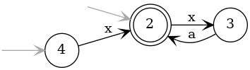
Figure 3: The Nfa $A_{0}$ for the regular expression $(x+\varepsilon).(x.a)^{*}$

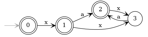
Figure 4: The accessible determinization $\det(A_{0})$ up to the renaming of states $[\{2,4\}/0,$$\{2,3\}/1,$$\{2\}/2,\{3\}/3]$.

As a running example, we consider the Nfa $A_{0}$ for the regular expression $(x+\varepsilon).(x.a)^{*}$ that is drawn as a labeled digraph in Figure 4: the nodes of the graph are the states and the labeled edges represent the transitions rules. The initial states are indicated by an ingoing arrow and the final state are doubly circled. The graph of the Dfa $\det(A_{0})$ obtained by accessible determinization is shown in Figure 4. It is given up to a renaming of the states that is given in the caption. Note that only $4$ out of the $2^{3}=8$ subsets are accessible, so the size increases only by a single state and two transitions rules in this example.

A regular schema over $\Sigma$ is a Dfa with the alphabet $\Sigma$. We next show how to use automata to define
regular queries on words. For this, any word is seen as a labeled digraph. The labeled digraph of the word $aab$, for instance, is drawn to the right. The set of nodes of the graph is the set of positions of the word $\mathit{pos}(w)=\{0,\ldots,n\}$ where $n$ is the length of $w$. Position $0$ is labeled by $start$, while all other positions are labeled by a single letter in $\Sigma$. A monadic query function on words with alphabet $\Sigma$ is a total function Q that maps some words $w\in\Sigma^{*}$ to a subset of position $\textbf{Q}(w)\subseteq\mathit{pos}(w)$. We say that a position $\pi\in\mathit{pos}(w)$ is selected by Q if $w\in\textit{dom}(\textbf{Q})$ and $\pi\in\textbf{Q}(w)$.

Let us fix a single variable $x$. Given a position $\pi$ of a word $w\in\Sigma^{*}$ let $w*[\pi/x]$ be the word obtained from $w$ by inserting $x$ after position $\pi$. We note that all words of the form $w*[\pi/x]$ contain a single occurrence of $x$. Such words are also called $V$-structures where $V=\{x\}$ (see e.g [straubing1994finite]).

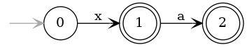
Figure 5: The schema-based cleaning of $\det(A_{0})$ with schema ${{words\textrm{-}one^{x}_{\Sigma}}}$.

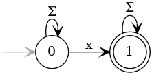
Figure 6: Schema ${{words\textrm{-}one^{x}_{\Sigma}}}$ with alphabet $\Sigma\uplus\{x\}$.

The set of all $V$-structures can be defined by the schema ${{words\textrm{-}one^{x}_{\Sigma}}}$ over $\Sigma\uplus\{x\}$ in Figure 6. It is natural to identify any total monadic query function Q with the language of $V$-structures $L_{\textbf{Q}}=\{w*[\pi/x]\mid w\in\Sigma^{*},\pi\in\textbf{Q}(w)\}$. This view permits us to define a subclass of total monadic query functions by automata. A (monadic) query automaton over $\Sigma$ is a Nfa $A$ with alphabet $\Sigma\uplus\{x\}$. It defines the unique total monadic query function Q such that $L_{\textbf{Q}}=\mathcal{L}(A)\cap\mathcal{L}({{words\textrm{-}one^{x}_{\Sigma}}})$. A position $\pi$ of a word $w\in\Sigma^{*}$ is thus selected by the query Q on $w$ if and only if the $V$-structure $w*[\pi/x]$ is recognized by $A$, i.e.:

$$\pi\in\textbf{Q}(w)\Leftrightarrow w*[\pi/x]\in\mathcal{L}(A)$$

A query function is called regular if it can be defined by some Nfa. It is well-known from the work of Büchi in the sixties [Buchi60] that the same class of regular query functions can be defined equivalently by monadic second-order logic.

We note that only the words satisfying the schema ${{words\textrm{-}one^{x}_{\Sigma}}}$ (the $V$-structures) are relevant for the query function Q of a query automaton $A$. The query automaton $A_{0}$ in Figure 4 for instance, defines the query function that selects the start position of the words $\varepsilon$ and $a$ and no other positions elsewhere. This is since the subset of $V$-structures recognized by $A_{0}$ is $x+x.a$. Note that the words $\varepsilon$ and $xxa$ do also belong to $\mathcal{L}(A_{0})$, but are not $V$-structures, and thus are irrelevant for the query function Q.

4 Schema-Based Cleaning

Schema-based cleaning was introduced only recently [Sakho] in order to reduce the size of automata on nested words. The idea is to remove all rules and states from an automaton that are not used to recognize any word satisfying the schema. Schema-based cleaning can be based on the accessible states of the product of the automaton with the schema. While this product may be larger than the automaton, the schema-based cleaning will always be smaller.

For illustration, the schema-based cleaning of Nfa $\det(A_{0})$ in Figure 4 with respect to schema ${{words\textrm{-}one^{x}_{\Sigma}}}$ is given in Figure 6. The only words recognized by both $\det(A_{0})$ and ${{words\textrm{-}one^{x}_{\Sigma}}}$ are $x$ and $xa$. For recognizing these two words, the automaton $\det(A_{0})$ does not need states $2$ and $3$, so they can be removed with all their transitions rules. Thereby, the word $xxa$ violating the schema is no more recognized after schema-based cleaning, while it was recognized by $\det(A_{0})$. Furthermore, note that the state $0$ needs no more to be final after schema-based cleaning. Therefore the word $\varepsilon$, which is recognized by the automaton but not by the schema, is no more recognized after schema-based cleaning. So schema-based cleaning may change the language of the automaton but only outside of the schema.

Interestingly, the Nfa $A_{0}$ in Figure 4 is schema-clean for schema ${{words\textrm{-}one^{x}_{\Sigma}}}$ too, even though it is not perfect, in that it recognizes the words $\varepsilon$ and $xxa$ which are rejected by the schema. The reason is that for recognizing the words $x$ and $xa$, which both satisfy the schema, all 3 states and all 4 transition rules of $A_{0}$ are needed. In contrast, we already noticed that the accessible determinization $\det(A_{0})$ in Figure 4 is not schema-clean for schema ${{words\textrm{-}one^{x}_{\Sigma}}}$. This illustrates that accessible determinization does not always preserve schema-cleanliness. In other words, schema-based cleaning may have a stronger cleaning effect after determinization than before.

$$\begin{array}[]{c}(q,s)\in I^{A\times S}\qquad(q,s)\in\mathcal{Q}^{A\times S}\lx@proof@logical@and q\in I^{A}s\in I^{S}\qquad(q,s)\in F^{A\times S}\lx@proof@logical@and q\in F^{A}s\in F^{S}(q,s)\in\mathcal{Q}^{A\times S}\\ \\ (q_{1},s_{1})\xrightarrow{a}(q_{2},s_{2})\in\Delta^{A\times S}\quad(q_{2},s_{2})\in\mathcal{Q}^{A\times S}\lx@proof@logical@and q_{1}\xrightarrow{a}q_{2}\in\Delta^{A}s_{1}\xrightarrow{a}s_{2}\in\Delta^{S}\quad(q_{1},s_{1})\in\mathcal{Q}^{A\times S}\par\end{array}$$

Figure 7: Accessible product $A\times S=(\Sigma,\mathcal{Q}^{A\times S},I^{A\times S},F^{A\times S},\Delta^{A\times S})$.

The schema-based cleaning of an automaton can be defined based on the accessible product of the automaton with the schema. The accessible product $A\times S$ of two Nfas $A$ and $S$ with alphabet $\Sigma$ is defined in Figure 7. This is the usual product, except that only accessible states are admitted. Clearly, $\mathcal{L}(A\times S)=\mathcal{L}(A)\cap\mathcal{L}(S)$. Let $\Pi_{A}(A\times S)$ be obtained from the accessible product by projecting away the second component. The schema-based cleaning of $A$ with respect to schema $S$ is this projection.

Definition 4.1.

$\mathit{scl}_{S}(A)=\Pi_{A}(A\times S)$.

$$\begin{array}[]{c}q\in I^{\Pi_{A}(A\times S)}(q,s)\in I^{A\times S}\qquad q\in\mathcal{Q}^{\Pi_{A}(A\times S)}(q,s)\in\mathcal{Q}^{A\times S}\qquad q\in F^{\Pi_{A}(A\times S)}(q,s)\in F^{A\times S}\qquad q_{1}\xrightarrow{a}q_{2}\in\Delta^{\Pi_{A}(A\times S)}(q_{1},s_{1})\xrightarrow{a}(q_{2},s_{2})\in\Delta^{A\times S}\end{array}$$

Figure 8: Projection $\Pi_{A}(A\times S)=(\Sigma,\mathcal{Q}^{\Pi_{A}(A\times S)},\Delta^{\Pi_{A}(A\times S)},I^{\Pi_{A}(A\times S)},F^{\Pi_{A}(A\times S)})$.

The fact that $A\times S$ is restricted to accessible states matches our intuition that all states of $\mathit{scl}_{S}(A)$ can be used to read some word in $\mathcal{L}(A)$ that satisfies schema $S$. This can be proven formally under the condition that all states of $A\times S$ are also co-accessible. Clearly, $\mathit{scl}_{S}(A)$ is obtained from $A$ by removing states, initial states, final states, and transitions rules. So it is smaller or equal in size $|\mathit{scl}_{S}(A)|\leq|A|$ and language $\mathcal{L}(\mathit{scl}_{S}(A))\subseteq\mathcal{L}(A)$. Still, schema-based cleaning preserves the language within the schema.

Proposition 4.2 ([Sakho]).

$\mathcal{L}(A)\cap\mathcal{L}(S)=\mathcal{L}(\mathit{scl}_{S}(A))\cap\mathcal{L}(S)$.

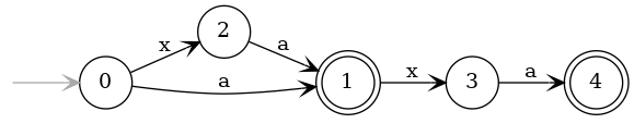
Figure 9: A Dfa that is schema-clean but not perfect for ${{words\textrm{-}one^{x}_{\Sigma}}}$.

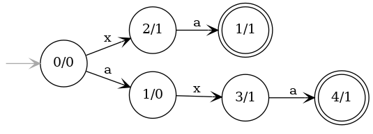
Figure 10: The accessible product with ${{words\textrm{-}one^{x}_{\Sigma}}}$ is schema-clean and perfect for ${{words\textrm{-}one^{x}_{\Sigma}}}$.

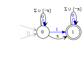
Figure 11: The dSha ${{one^{x}_{\Sigma}}}$ with alphabet $\Sigma\uplus\{x,\neg x\}$.

Schema-clean deterministic automata may still not be perfect, in that they may recognize some words outside the schema. This happens for Dfas if some state of is reached, both, by a word satisfying the schema and another word that does not satisfy the schema. An example for a Dfa that is schema-clean but not perfect for ${{words\textrm{-}one^{x}_{\Sigma}}}$ is given in Figure 11. It is not perfect since it accepts the non $V$-structure $xaxa$. The problem is that state $1$ can be reached by the words $a$ and $xa$, so one cannot infer from being in state $1$ whether some $x$ was read or not. If one wants to avoid this, one can use the accessible product of the Dfa with the schema instead. In the example, this yields the Dfa in Figure 11 that is schema-clean and perfect for ${{words\textrm{-}one^{x}_{\Sigma}}}$.

Proposition 4.3 (Folklore).

For any two Dfas $A$ and $S$ with alphabet $\Sigma$ the accessible product $A\times S$ can be computed in expected amortized time $O(|\mathcal{Q}^{A\times S}||\Sigma|+|A|+|S|)$.

Proof 4.4.

An algorithm to compute the fixed points of the inference rules for the accessible product $A\times S$ in Figure 7 can be organized such that only accessible states are considered (similarly to semi-naive datalog evaluation). This algorithm is presented in Figure 12. It dynamically generates the set of rules $Rules$ by using perfect dynamic hashing [DBLP:journals/siamcomp/DietzfelbingerKMHRT94]. Testing set membership is in time $O(1)$ and the addition of elements to the set is in expected amortized time $O(1)$. The algorithm uses a stack, $Agenda$, to memoize all new pairs $(q_{1},s_{1})\in\mathcal{Q}^{A\times S}$ that need to be processed, and a hash set $Store$ that saves all processed states $\mathcal{Q}^{A\times S}$. We aim not to push the same pair more than once in the $Agenda$. For this, membership to the $Store$ is checked before an element is pushed to the $Agenda$. For each pair popped from the stack $Agenda$, the algorithm does the following: for each letter $a\in\Sigma$ it computes the sets $Q=\{q_{2}\mid q_{1}\xrightarrow{a}q_{2}\in\Delta^{A}\}$ and $R=\{s_{2}\mid s_{1}\xrightarrow{a}s_{2}\in\Delta^{S}\}$ and then adds the subset of states of $Q\times R$ that were not stored in the hash set $Store$ to the agenda. Since $A$ and $S$ are deterministic, there is at most one such pair, so the time for treating one pair on the agenda is in expected amortized time $O(|\Sigma|)$. The overall number of elements in the agenda will be $|\mathcal{Q}^{A\times S}|$. Note that $Q$ and $R$ can be computed in $O(1)$ after preprocessing $A$ and $S$ in time $O(|A|+|S|)$. Therefore, we will have a total time of the algorithm in $O(|\mathcal{Q}^{A\times S}||\Sigma|+|A|+|S|)$.

Corollary 4.5.

For any two Dfas $A$ and $S$ with alphabet $\Sigma$ schema-based cleaning $\mathit{scl}_{S}(A)$ can be computed in expected amortized time $O(|\mathcal{Q}^{A\times S}||\Sigma|+|A|+|S|)$.

Proof 4.6.

By Definition 4.1 it is sufficient to compute the projection of the accessible product $A\times S$. By Proposition 4.3 the product can be computed in time $O(|\mathcal{Q}^{A\times S}||\Sigma|+|A|+|S|)$. Its size cannot be larger than its computation time. The projection can be computed in linear time in the size of $A\times S$, so the overall time is in $O(|\mathcal{Q}^{A\times S}||\Sigma|+|A|+|S|)$ too.

⬇

1fun $A\times S$ =

2 let $Store=hashset.new(\emptyset)$ and $Agenda=list.new()$ and $Rules=hashset.new(\emptyset)$

3 if $\mathit{init}^{A}=\{q_{0}\}$ and $\mathit{init}^{S}=\{s_{0}\}$ then $Agenda.add((q_{0},s_{0}))$

4 while $Agenda.notEmpty()$ do

5 let $(q_{1},s_{1})=Agenda.pop()$

6 for $a\in\Sigma$ do

7 let $Q=\{q_{2}\mid q_{1}\xrightarrow{a}q_{2}\in\Delta^{A}\}$ $R=\{s_{2}\mid s_{1}\xrightarrow{a}s_{2}\in\Delta^{S}\}$

8 for $q_{2}\in Q$ and $s_{2}\in R$ do

9 $Rules.add((q_{1},s_{1})\xrightarrow{a}(q_{2},s_{2}))$

10 if not $Store.member((q_{2},s_{2}))$

11 then $Store.add((q_{2},s_{2}))$ $Agenda.push((q_{2},s_{2}))$

12 let $\mathit{init}^{A\times S}=\{(q_{0},s_{0})\mid(q_{0},s_{0})\in Store\}$ and $F^{A\times S}=\{(q,s)\mid(q,s)\in Store,q\in F^{A},s\in F^{S}\}$

13 return $(\Sigma,Store.toSet(),Rules.toSet(),\mathit{init}^{A\times S},F^{A\times S})$

Figure 12: An algorithm computing the accessible product of Dfas $A$ and $S$.

5 Schema-Based Determinization

Schema-based cleaning after determinization becomes impossible in practice if the automaton obtained by determinization is too big. We therefore show next how to integrate schema-based cleaning into automata determinization directly.

The schema-based determinization of $A$ with respect to schema $S$ extends on accessible determinization $\det(A)$. The idea is to run the schema $S$ in parallel with $\det(A)$, in order to keep only those state $Q\in\mathcal{Q}^{\det(A)}$ that can be aligned to some state $s\in\mathcal{Q}^{S}$. In this case we write $Q\sim s$.

$$Q\in I^{\mathit{det}_{S}(A)}\quad Q\sim s\lx@proof@logical@and Q\in I^{det(A)}I^{S}=\{s\}\qquad Q\in\mathcal{Q}^{\mathit{det}_{S}(A)}Q\sim s\qquad Q\in\mathit{F}^{\mathit{det}_{S}(A)}Q\in\mathit{F}^{\det(A)}\qquad s\in\mathit{F}^{S}\qquad Q\sim s$$

$$Q\xrightarrow{a}Q^{\prime}\in\Delta^{\mathit{det}_{S}(A)}\qquad Q^{\prime}\sim s^{\prime}\begin{array}[]{c}Q\xrightarrow{a}Q^{\prime}\in\Delta^{det(A)}\qquad Q\sim s\qquad s\xrightarrow{a}s^{\prime}\in\Delta^{S}\end{array}$$

Figure 13: Schema-based determ. $\mathit{det}_{S}(A)=(\Sigma,\mathcal{Q}^{\mathit{det}_{S}(A)},\Delta^{\mathit{det}_{S}(A)},I^{\mathit{det}_{S}(A)},F^{\mathit{det}_{S}(A)})$.

The schema-determinization $\mathit{det}_{S}(A)$ is defined in Figure 13. The automaton $\mathit{det}_{S}(A)$ permits to go from any subset $Q\in\mathcal{Q}^{\det(A)}$ and letter $a\in\Sigma$ to the set of states $Q^{\prime}=a^{\Delta^{\det(A)}}(Q)$, under the condition that there exists schema states $s,s^{\prime}\in\mathcal{Q}^{S}$ such that $Q\sim s$ and $s\xrightarrow{a}s^{\prime}$. In this case $Q^{\prime}\sim s^{\prime}$ is inferred.

keytheoremproof[theoremproof]Claim

theoTheorem

[Correctness] $\mathit{det}_{S}(A)=\mathit{scl}_{S}(\det(A))$ for any Nfa $A$ and Dfa $S$ with the same alphabet.

The theorem states that schema-based determinization yields the same result as accessible determinization followed by schema-based cleaning.

For the correctness proof we collapse the two systems of inference rules for accessible products and projection into a single rule system. This yields the rule systems for schema-based cleaning in Figure 14.

$$\begin{array}[]{c}q\in I^{\widehat{\mathit{scl}}_{S}(A)}\quad(q,s)\in\mathcal{Q}^{A\widehat{\times}S}q\in I^{A}\quad s\in I^{S}\qquad q\in F^{\widehat{\mathit{scl}}_{S}(A)}\lx@proof@logical@and q\in F^{A}s\in F^{S}(q,s)\in\mathcal{Q}^{A\widehat{\times}S}\\[1.99997pt] q\in\mathcal{Q}^{\widehat{\mathit{scl}}_{S}(A)}(q,s)\in\mathcal{Q}^{A\widehat{\times}S}\qquad q_{1}\xrightarrow{a}q_{2}\in\Delta^{\widehat{\mathit{scl}}_{S}(A)}\quad(q_{2},s_{2})\in\mathcal{Q}^{A\widehat{\times}S}q_{1}\xrightarrow{a}q_{2}\in\Delta^{A}\quad s_{1}\xrightarrow{a}s_{2}\in\Delta^{S}\quad(q_{1},s_{1})\in\mathcal{Q}^{A\widehat{\times}S}\end{array}$$

$$\widehat{\mathit{scl}}_{S}(A)=(\Sigma,\mathcal{Q}^{\widehat{\mathit{scl}}_{S}(A)},\Delta^{\widehat{\mathit{scl}}_{S}(A)},I^{\widehat{\mathit{scl}}_{S}(A)},F^{\widehat{\mathit{scl}}_{S}(A)})$$

Figure 14: A collapsed rule systems for schema-based cleaning $\widehat{\mathit{scl}}_{S}(A)$.

⬇

1fun detS($A$,$S$) =

2 let $Store=hashset.new(\emptyset)$ and $Agenda=list.new()$ and $Rules=hashset.new(\emptyset)$

3 if $\mathit{init}^{A}\not=\emptyset$ and $\mathit{init}^{S}=\{s_{0}\}$ then $Agenda.add(\mathit{init}^{A}\sim s_{0})$

4 while $Agenda.notEmpty()$ do

5 let $(Q_{1}\sim s_{1})=Agenda.pop()$

6 for $a\in\Sigma$ do

7 let $P=\{Q_{2}\mid Q_{1}\xrightarrow{a}Q_{2}\in\Delta^{\det(A)}\}$ and $R=\{s_{2}\mid s_{1}\xrightarrow{a}s_{2}\in\Delta^{S}\}$

8 for $Q_{2}\in P$ and $s_{2}\in R$ do $Rules.add(Q_{1}\xrightarrow{a}Q_{2})$

9 if not $Store.member(Q_{2}\sim s_{2})$

10 then $Store.add(Q_{2}\sim s_{2})$ $Agenda.push(Q_{2}\sim s_{2})$

11 let $\mathit{init}^{\mathit{det}_{S}(A)}=\{Q\mid Q\sim s\in Store,Q\cap\mathit{init}^{A}\not=\emptyset\}$ and $F^{\mathit{det}_{S}(A)}=\{Q\mid Q\sim s\in Store,Q\cap F^{A}\not=\emptyset\}$

12 return $(\Sigma,Store.toSet(),Rules.toSet(),\mathit{init}^{\mathit{det}_{S}(A)},F^{\mathit{det}_{S}(A)})$

Figure 15: An algorithm for schema-based determinization $\mathit{det}_{S}(A)$ of an Nfa $A$ and a Dfa schema $S$.

The rules there define the automaton $\widehat{\mathit{scl}}_{S}(A)$, that we annotate with a hat, in order to distinguish it from the previous automaton $\mathit{scl}_{S}(A)$. The rules also infer judgements $(q,s)\in\mathcal{Q}^{A\widehat{\times}S}$ that we distinguish by a hat from the previous judgments $(q,s)\in\mathcal{Q}^{A\times S}$ of the accessible product. The next proposition shows that the system of collapsed inference rules indeed redefines the schema-based cleaning.

For any two Nfas $A$ and $S$ with the same alphabet:

$$\mathit{scl}_{S}(A)=\widehat{\mathit{scl}}_{S}(A)\quad\text{\ and\ }\quad\mathcal{Q}^{A\times S}=\mathcal{Q}^{A\widehat{\times}S}$$

Proof 5.1.

The two equations are shown by the following four lemmas. The judgements with a hat there are to be inferred by the collapsed system of inference rules in Figure 14, while the other judgments are to be inferred with the rule system for accessible products in Figure 7.

$q\in I^{\widehat{\mathit{scl}}_{S}(A)}$ iff $q\in I^{\mathit{scl}_{S}(A)}$.

Proof 5.2.

The rule systems of accessible product, projection, and the collapsed system can be used as following :

$$q\in I^{\widehat{\mathit{scl}}_{S}(A)}q\in I^{A}\quad s\in I^{S}\quad q\in I^{\mathit{scl}_{S}(A)}(q,s)\in I^{A\times S}\lx@proof@logical@and q\in I^{A}s\in I^{S}$$

$(q,s)\in\mathcal{Q}^{A\widehat{\times}S}$ iff $(q,s)\in\mathcal{Q}^{A\times S}$.

Proof 5.3.

We proof for all $n\geq 0$ that if $(q,s)\in\mathcal{Q}^{A\widehat{\times}S}$ has a proof tree of size $n$ then there exists a proof tree for $(q,s)\in\mathcal{Q}^{A\times S}$. The proof is by induction on $n$.

In the case of the rules of the initial states, $(q,s)\in\mathcal{Q}^{A\widehat{\times}S}$ is inferred directly whenever $(q,s)\in\mathcal{Q}^{A\times S}$ and vice versa, using the following:

$$(q,s)\in I^{A\times S}\qquad(q,s)\in\mathcal{Q}^{A\times S}\lx@proof@logical@and q\in I^{A}s\in I^{S}\qquad q\in I^{\widehat{\mathit{scl}}_{S}(A)}\quad(q,s)\in\mathcal{Q}^{A\widehat{\times}S}q\in I^{A}\quad s\in I^{S}$$

If $(q,s)\in\mathcal{Q}^{A\widehat{\times}S}$ is inferred by the internal rule of the collapsed rule system in Figure 14. Then the proof tree has the following form for some proof tree $T_{1}$:

$$(q_{2},s_{2})\in\mathcal{Q}^{A\widehat{\times}S}q_{1}\xrightarrow{a}q_{2}\in\Delta^{A}\quad s_{1}\xrightarrow{a}s_{2}\in\Delta^{S}\quad(q_{1},s_{1})\in\mathcal{Q}^{A\widehat{\times}S}T_{1}$$

This shows that there is a smaller proof tree $T_{1}$ for inferring $(q_{1},s_{1})\in\mathcal{Q}^{A\widehat{\times}S}$. So by induction hypothesis applied to $T_{1}$, there exists a proof tree $T^{\prime}_{1}$ for inferring $(q_{1},s_{1})\in\mathcal{Q}^{A\times S}$ with the proof system of accessible products in Figure 7:

$$(q_{1},s_{1})\in\mathcal{Q}^{A\times S}T^{\prime}_{1}$$

Therefore, we also have the following proof tree for $(q_{2},s_{2})\in\mathcal{Q}^{A\times S}$ with the internal rule for the accessible product:

$$(q_{2},s_{2})\in\mathcal{Q}^{A\times S}q_{1}\xrightarrow{a}q_{2}\in\Delta^{A}\quad s_{1}\xrightarrow{a}s_{2}\in\Delta^{S}\quad(q_{1},s_{1})\in\mathcal{Q}^{A\times S}T^{\prime}_{1}$$

For the inverse direction, if $(q,s)\in\mathcal{Q}^{A\times S}$ is inferred by the internal rule of the accessible product rule system in Figure 7. Then the proof tree has the following form for some proof tree $T_{1}$:

$$(q_{2},s_{2})\in\mathcal{Q}^{A\times S}q_{1}\xrightarrow{a}q_{2}\in\Delta^{A}\quad s_{1}\xrightarrow{a}s_{2}\in\Delta^{S}\quad(q_{1},s_{1})\in\mathcal{Q}^{A\times S}T_{1}$$

This means that there is a smaller proof tree $T_{1}$ for inferring $(q_{1},s_{1})\in\mathcal{Q}^{A\times S}$. By induction hypothesis applied to $T_{1}$, there exists a proof tree $T^{\prime}_{1}$ for inferring $(q_{1},s_{1})\in\mathcal{Q}^{A\widehat{\times}S}$ with the collapsed system in Figure 14:

$$(q_{1},s_{1})\in\mathcal{Q}^{A\widehat{\times}S}T^{\prime}_{1}$$

which leads to the following proof tree for $(q_{2},s_{2})\in\mathcal{Q}^{A\times S}$ with the internal rule for the collapsed system:

$$(q_{2},s_{2})\in\mathcal{Q}^{A\widehat{\times}S}q_{1}\xrightarrow{a}q_{2}\in\Delta^{A}\quad s_{1}\xrightarrow{a}s_{2}\in\Delta^{S}\quad(q_{1},s_{1})\in\mathcal{Q}^{A\widehat{\times}S}T^{\prime}_{1}$$

$q_{1}\xrightarrow{a}q_{2}\in\Delta^{\widehat{\mathit{scl}}_{S}(A)}$ iff $q_{1}\xrightarrow{a}q_{2}\in\Delta^{\mathit{scl}_{S}(A)}$.

Proof 5.4.

We prove for all $n\geq 0$ that, if $q_{1}\xrightarrow{a}q_{2}\in\Delta^{\widehat{\mathit{scl}}_{S}(A)}$ has a proof tree of size $n$, then there exists a proof tree for $q_{1}\xrightarrow{a}q_{2}\in\Delta^{\mathit{scl}_{S}{A}}$ and vice versa. The proof is by induction on $n$.

If $q_{1}\xrightarrow{a}q_{2}\in\Delta^{\widehat{\mathit{scl}}_{S}(A)}$ is inferred by the internal rule of the collapsed system, the proof tree will have the following for some tree $T_{1}$:

$$q_{1}\xrightarrow{a}q_{2}\in\Delta^{\widehat{\mathit{scl}}_{S}(A)}q_{1}\xrightarrow{a}q_{2}\in\Delta^{A}\quad s_{1}\xrightarrow{a}s_{2}\in\Delta^{S}\quad(q_{1},s_{1})\in\mathcal{Q}^{A\widehat{\times}S}T_{1}$$

By Lemma 5 and the rule of internal rules of the accessible product rule system:

$$(q_{1},s_{1})\xrightarrow{a}(q_{2},s_{2})\in\Delta^{A\times S}q_{1}\xrightarrow{a}q_{2}\in\Delta^{A}\quad s_{1}\xrightarrow{a}s_{2}\in\Delta^{S}\quad(q_{1},s_{1})\in\mathcal{Q}^{A\times S}T^{\prime}_{1}$$

For the inverse direction, if $q_{1}\xrightarrow{a}q_{2}\in\Delta^{\mathit{scl}_{S}(A)}$ is inferred by the internal rule of the accessible product, the proof tree will have the following for some tree $T_{1}$:

$$q_{1}\xrightarrow{a}q_{2}\in\Delta^{\mathit{scl}_{S}(A)}(q_{1},s_{1})\xrightarrow{a}(q_{2},s_{2})\in\Delta^{A\times S}q_{1}\xrightarrow{a}q_{2}\in\Delta^{A}\quad s_{1}\xrightarrow{a}s_{2}\in\Delta^{S}\quad(q_{1},s_{1})\in\mathcal{Q}^{A\times S}T_{1}$$

By lemma 5 and the rule of internal rules of the collapsed system:

$$q_{1}\xrightarrow{a}q_{2}\in\Delta^{\widehat{\mathit{scl}}_{S}(A)}q_{1}\xrightarrow{a}q_{2}\in\Delta^{A}\quad s_{1}\xrightarrow{a}s_{2}\in\Delta^{S}\quad(q_{1},s_{1})\in\mathcal{Q}^{A\times S}T^{\prime}_{1}$$

$q\in\mathcal{Q}^{\widehat{\mathit{scl}}_{S}(A)}$ iff $q\in\mathcal{Q}^{\mathit{scl}_{S}(A)}$ and $q\in F^{\widehat{\mathit{scl}}_{S}(A)}$ iff $q\in F^{\mathit{scl}_{S}(A)}$.

Proof 5.5.

We start proving $q\in\mathcal{Q}^{\widehat{\mathit{scl}}_{S}(A)}$ iff $q\in\mathcal{Q}^{\mathit{scl}_{S}(A)}$. By Lemma 5, and rules of construction of the accessible product, projection, and collapsed systems, this lemma holds for some proof trees $T$ and $T^{\prime}$ as follows:

$$q\in\mathcal{Q}^{\mathit{scl}_{S}(A)}(q,s)\in\mathcal{Q}^{A\times S}T\quad q\in\mathcal{Q}^{\widehat{\mathit{scl}}_{S}(A)}T^{\prime}$$

Finally, we show $q\in F^{\widehat{\mathit{scl}}_{S}(A)}$ iff $q\in F^{\mathit{scl}_{S}(A)}$. Using Lemma 5, there exists some proof trees $T$ and $T^{\prime}$ that infers $(q,s)\in\mathcal{Q}^{A\times S}$ and $(q,s)\in\mathcal{Q}^{A\widehat{\times}S}$ in both ways and therefore having the following form of rules:

$$q\in F^{\widehat{\mathit{scl}}_{S}(A)}\lx@proof@logical@and q\in F^{A}s\in F^{S}(q,s)\in\mathcal{Q}^{A\widehat{\times}S}T\quad q\in F^{\mathit{scl}_{S}(A)}(q,s)\in F^{A\times S}\lx@proof@logical@and q\in F^{A}s\in F^{S}(q,s)\in\mathcal{Q}^{A\times S}T^{\prime}$$

Proof of Correctness Theorem 13. Instantiating the system of collapsed rules for schema-based cleaning from Figure 14 with $\det(A)$ for $A$ yields the rule system in Figure 16.

$$\begin{array}[]{c}Q\in I^{\widehat{\mathit{scl}}_{S}(det(A))}\quad(Q,s)\in\mathcal{Q}^{det(A)\widehat{\times}S}Q\in I^{det(A)}\quad s\in I^{S}\quad Q\in F^{\widehat{\mathit{scl}}_{S}(det(A))}\lx@proof@logical@and Q\in F^{det(A)}s\in F^{S}(Q,s)\in\mathcal{Q}^{det(A)\times S}\\[1.99997pt] Q\in\mathcal{Q}^{\widehat{\mathit{scl}}_{S}(det(A))}(Q,s)\in\mathcal{Q}^{det(A)\widehat{\times}S}\quad Q_{1}\xrightarrow{a}Q_{2}\in\Delta^{\widehat{\mathit{scl}}_{S}(det(A))}\quad(Q_{2},s_{2})\in\mathcal{Q}^{det(A)\widehat{\times}S}Q_{1}\xrightarrow{a}Q_{2}\in\Delta^{det(A)}\quad s_{1}\xrightarrow{a}s_{2}\in\Delta^{S}\quad(Q_{1},s_{1})\in\mathcal{Q}^{det(A)\times S}\end{array}$$

$$\widehat{\mathit{scl}}_{S}(det(A))=(\Sigma,\mathcal{Q}^{\widehat{\mathit{scl}}_{S}(det(A))},\Delta^{\widehat{\mathit{scl}}_{S}(det(A))},I^{\widehat{\mathit{scl}}_{S}(det(A))},F^{\widehat{\mathit{scl}}_{S}(det(A))})$$

Figure 16: Instantiation of the collapsed rules for schema-based cleaning from Figure 14 with $\det(A)$.

We can identify the instantiated collapsed system for $\widehat{\mathit{scl}}_{S}(det(A))$ with that for $\mathit{det}_{S}(A)$ in Figure 13, by identifying the judgements $(Q,s)\in\mathcal{Q}^{det(A)\widehat{\times}S}$ with judgments $Q\sim s$. After renaming the predicates, the inference rules for the corresponding judgments are the same. Hence $\widehat{\mathit{scl}}_{S}(det(A))=\mathit{det}_{S}(A)$, so that Proposition 5 implies $\mathit{scl}_{S}(det(A))=\mathit{det}_{S}(A)$. ∎

Proposition 5.6.

The schema-based determinization $\mathit{det}_{S}(A)$ for a Nfa $A$ and a Dfa $S$ over $\Sigma$ can be computed in expected amortized time $O(|\mathcal{Q}^{\det(A)\times S}||\Sigma|+|\mathcal{Q}^{\mathit{det}_{S}(A)}||\Delta^{A}|+|A|+|S|)$.

Proof 5.7.

An algorithm computing the fixed points of the inference rules of schema-based determinization from Figure 13 is given in Figure 15. It refines the algorithm computing the accessible product with on-the-fly determinization and projection.

On the stack $Agenda$, the algorithm stores alignments $Q\sim s$ such that $(Q,s)\in\mathcal{Q}^{\det(A)\times S}$ that were not considered before. Transition rules of $\mathit{det}_{S}(A)$ are collected in hash set $\mathit{Rules}$, using the dynamic perfect hashing aforementioned. The alignments $Q_{1}\sim s_{1}$ popped from the agenda are processed as follows: For any letter $a\in\Sigma$, the sets $R=\{Q_{2}\mid Q_{1}\xrightarrow{a}Q_{2}\in\Delta^{\det(A)}\}$ and $P=\{s_{2}\mid s_{1}\xrightarrow{a}s_{2}\in\Delta^{S}\}$ are computed. One then pushes all new pairs $Q_{2}\sim s_{2}$ with $Q_{2}\in P$ and $s_{2}\in R$ into the agenda, and adds $Q_{1}\xrightarrow{a}Q_{2}$ to the set $\mathit{Rules}$. Since $S$ and $\det(A)$ are deterministic there is at most one pair $(Q,s)\in P\times R$ for $Q_{1}$ and $s_{1}$. So the time for treating one pair on the agenda is in $O(|\Sigma|)$ plus the time for building the needed transition rules of $\det(A)$ from $\Delta^{A}$ on the fly. The time for the on the fly computation of transition rules of $\det(A)$ is in time $O(|\mathcal{Q}^{\mathit{det}_{S}(A)}||\Delta^{A}|)$. The overall number of pairs on the agenda is at most $|\mathcal{Q}^{\det(A)\times S}|$ so the main while loop of the algorithm requires time in $O(|\mathcal{Q}^{\det(A)\times S}||\Sigma|)$ apart from on the fly determinization.

By Proposition 3.2, computing $\det(A)$ requires time $O(|\mathcal{Q}^{det(A)}|\ |\Delta^{A}|+|A|)$. Therefore, with Proposition 4.3, the accessible product $\det(A)\times S$ can be computed from $A$ and $S$ in time $O(|\mathcal{Q}^{\det(A)\times S}||\Sigma|+|\mathcal{Q}^{det(A)}|\ |\Delta^{A}|+|A|+|S|)$. Since $\mathcal{Q}^{\mathit{det}_{S}(A)}\subseteq\mathcal{Q}^{\det(A)}$ the proposition shows that schema-based determinization is at most as efficient in the worst case as accessible determinization followed by schema-based cleaning. If $|\mathcal{Q}^{\det(A)\times S}||\Sigma|<|\mathcal{Q}^{\det(A)}||\Delta^{A}|$ then it is more efficient, since schema-based determinization avoids the computation of $\det(A)$ all over. Instead, it only computes the accessible product $\det(A)\times S$, which may be way smaller, since exponentially many states of $\det(A)$ may not be aligned to any state of $S$. Sometimes, however, the accessible product may be bigger. In this case, schema-based determinization may be more costly than pure accessible determinization, not followed by schema-based cleaning.

6 Stepwise Hedge Automata for Nested Words

We next recall Shas [Sakho] for defining languages of nested words, regular schemas and queries. Nested words generalize on words by adding parenthesis that must be well-nested. While containing words natively, they also generalize on unranked trees, and hedges. We restrict ourselves to nested words with a single pair of opening and closing parenthesis $\boldsymbol{\langle}$ and $\boldsymbol{\rangle}$. Nested words over a finite alphabet $\Sigma$ of internal letters have the following abstract syntax.

$$\begin{array}[]{rcl}w,w^{\prime}\in\mathcal{N}_{\Sigma}&::=&\varepsilon\mid a\mid\boldsymbol{\langle}w\boldsymbol{\rangle}\mid w\cdot w^{\prime}\qquad\text{ where }a\in\Sigma\end{array}$$

We assume that concatenation $\cdot$ is associative and that the empty word $\varepsilon$ is a neutral element, that is $w\cdot(w^{\prime}\cdot w^{\prime\prime})=(w\cdot w^{\prime})\cdot w^{\prime\prime}$ and $\varepsilon\cdot w=w=w\cdot\varepsilon$. Nested words can be identified with hedges, i.e., words of unranked trees and letters from $\Sigma$. Seen as a graph, the inner nodes are labeled by the tree constructor $\boldsymbol{\langle}\boldsymbol{\rangle}$ and the leafs by symbols in $\Sigma$ or the tree constructor. For instance $\boldsymbol{\langle}a\cdot\boldsymbol{\langle}b\boldsymbol{\rangle}\cdot\varepsilon\boldsymbol{\rangle}\cdot c\cdot\boldsymbol{\langle}d\cdot\boldsymbol{\langle}\varepsilon\boldsymbol{\rangle}\boldsymbol{\rangle}$ corresponds to the hed-

for tree=s sep=(3-level)*0.6mm [$\boldsymbol{\langle}\boldsymbol{\rangle}$ [a] [$\boldsymbol{\langle}\boldsymbol{\rangle}$ [b]]] [c] [$\boldsymbol{\langle}\boldsymbol{\rangle}$ [d] [$\boldsymbol{\langle}\boldsymbol{\rangle}$]]

ge on the right. A nested word of type tree has the form $\boldsymbol{\langle}h\boldsymbol{\rangle}$. Note that dangling parentheses are ruled out and that labeled parentheses can be simulated by using internal letters. xmldocuments are labeled unranked trees, for instance: $\boldsymbol{\langle}a\ name=``uff"\boldsymbol{\rangle}\boldsymbol{\langle}b\boldsymbol{\rangle}isgaga\boldsymbol{\langle}d/\boldsymbol{\rangle}\boldsymbol{\langle}/b\boldsymbol{\rangle}\boldsymbol{\langle}c/\boldsymbol{\rangle}\boldsymbol{\langle}/a\boldsymbol{\rangle}$. Labeled unranked trees satisfying the xmldata model can be represented as nested words over an alphabet that contains the xmlnode-types $(elem,attr,text,$ $\ldots)$, the xmlnames of the document $(a,\ldots,d,name)$, and the characters of the data values, say UTF8. For the above example, we get the nested word $\boldsymbol{\langle}elem\cdot a\cdot\boldsymbol{\langle}attr\cdot name\cdot u\cdot f\cdot f\boldsymbol{\rangle}\boldsymbol{\langle}elem\cdot b\cdot\boldsymbol{\langle}text\cdot i\cdot s\cdot g\cdot a\cdot g\cdot a\boldsymbol{\rangle}\boldsymbol{\langle}elem\cdot d\boldsymbol{\rangle}\boldsymbol{\rangle}\boldsymbol{\langle}elem\cdot c\boldsymbol{\rangle}\boldsymbol{\rangle}$

Definition 6.1.

A Sha is a tuple $A=(\Sigma,\mathcal{Q},\Delta,I,F)$ where $\Delta=(\Delta^{\prime},@^{\Delta},\boldsymbol{\langle}\boldsymbol{\rangle}^{\Delta})$ such that $(\Sigma,\mathcal{Q},\Delta^{\prime},I,F)$ is a Nfa, $\boldsymbol{\langle}\boldsymbol{\rangle}^{\Delta}\subseteq\mathcal{Q}$ is a set of tree initial states and $@^{\Delta}\subseteq\mathcal{Q}^{3}$ a set of apply rules.

Shas can be drawn as graphs while extending on the graphs of Nfas. A tree initial state $q\in\boldsymbol{\langle}\boldsymbol{\rangle}^{\Delta}$ is drawn as a node $\xrightarrow{\langle\rangle}\leavevmode\hbox to16.48pt{\vbox to16.48pt{\text{[drawing]}}}$ with an incoming tree arrow. An applyrule $(q_{1},q,q_{2})\in@^{\Delta}$ is drawn as a blue edge $\leavevmode\hbox to10.26pt{\vbox to10.26pt{\text{[drawing]}}}{\color[rgb]{0,0,1}\xrightarrow{q}}\leavevmode\hbox to10.26pt{\vbox to10.26pt{\text{[drawing]}}}$ that is labeled by a state $q\in\mathcal{Q}$ rather than a letter $a\in\Sigma$. It states that a nested word in state $q_{1}$ can be extended by a tree in state $q$ and become a nested word in state $q_{2}$.

For instance, the Sha ${{one^{x}_{\Sigma}}}$ is drawn graphically in Figure 11. It accepts all nested words over $\Sigma\uplus\{x,\neg x\}$ that contain exactly one occurrence of letter $x$. Compared to the Nfa ${{words\textrm{-}one^{x}_{\Sigma\uplus\{\neg x\}}}}$ from Figure 6, the Sha ${{one^{x}_{\Sigma}}}$ contains three additional apply rules $(0,0,0)$, $(0,1,1)$, $(1,0,1)\in@^{\Delta^{{one^{x}_{\Sigma}}}}$ for reading the states assigned to subtrees. The state $0$ is chosen as the single tree initial state.

Transitions for Nfas on words can be lifted to transitions for Shas of the form $q\xrightarrow{w}q^{\prime}\text{ wrt }\Delta$ where $w\in\mathcal{N}_{\Sigma}$ and $q,q^{\prime}\in\mathcal{Q}$. For this, we add the following inference rule to the previous rules for Nfas:

$$q_{1}\xrightarrow{\langle w\rangle}q_{2}\text{ wrt }\Delta q^{\prime}\in\boldsymbol{\langle}\boldsymbol{\rangle}^{\Delta}\qquad q^{\prime}\xrightarrow{w}q\text{ wrt }\Delta\qquad(q_{1},q,q_{2})\in@^{\Delta}$$

The rule says that a tree $\langle w\rangle$ can transit from a state $q_{1}$ to a state $q_{2}$ if there is an apply rule $(q_{1},q,q_{2})\in@^{\Delta}$ so that $w$ can transit from some tree initial state $q^{\prime}\in\boldsymbol{\langle}\boldsymbol{\rangle}^{\Delta}$ to $q$. Otherwise, the language $\mathcal{L}(A)$ of nested words accepted by a Sha $A$ is defined as in the case of Nfas.

Definition 6.2.

A Sha $(\Sigma,\mathcal{Q},\Delta,I,F)$ is deterministic or equivalently a dSha if it satisfies:

• $I$ and $\boldsymbol{\langle}\boldsymbol{\rangle}^{\Delta}$ both contain at most one element,

• $a^{\Delta}$ is a partial function from $\mathcal{Q}$ to $\mathcal{Q}$ for all $a\in\Sigma$, and

• $@^{\Delta}$ is a partial function from $\mathcal{Q}\times\mathcal{Q}$ to $\mathcal{Q}$.

Note that if $A$ is a dSha and $\Delta=(\Delta^{\prime},@^{\Delta},\boldsymbol{\langle}\boldsymbol{\rangle}^{\Delta})$ then $A^{\prime}=(\Sigma,\mathcal{Q},\Delta^{\prime},I,F)$ is a Dfa. Conversely any Dfa $A^{\prime}$ defines a dSha with $@^{\Delta}=\emptyset$ and $I=\emptyset$. For instance, the Sha ${{one^{x}_{\Sigma}}}$ in Figure 11 contains the Dfa ${{words\textrm{-}one^{x}_{\Sigma\uplus\{\neg x\}}}}$ from Figure 6 with $\Sigma$ instantiated by $\Sigma\uplus\{x\}$.

A schema for nested words over $\Sigma$ is a dSha over $\Sigma$. Note that schemas for nested words generalize over schemas of words, since dShas generalize on Dfas.

$$\boldsymbol{\langle}\boldsymbol{\rangle}^{\Delta^{A}}\in\mathcal{Q}^{\det(A)}\boldsymbol{\langle}\boldsymbol{\rangle}^{\Delta^{A}}\not=\emptyset\qquad Q_{1}@Q_{2}\to Q^{\prime}\in\Delta^{det(A)}\qquad Q^{\prime}\in\mathcal{Q}^{\det(A)}\begin{array}[]{c}Q_{1}\in\mathcal{Q}^{\det(A)}\qquad Q_{2}\in\mathcal{Q}^{\det(A)}\\ Q^{\prime}=\{q^{\prime}\in\mathcal{Q}^{A}\mid q_{1}@q_{2}\to q^{\prime}\in\Delta^{A},\ q_{1}\in Q_{1},q_{2}\in Q_{2}\}\not=\emptyset\end{array}$$

Figure 17: Accessible determinization $\det(A)$ lifted from Nfas to Shas.

⬇

1fun detSHA(A) =

2 let $Store=hashset.new(\emptyset)$

3 let $Agenda=list.new()$ and $Rules=hashset.new(\emptyset)$

4 if $\mathit{init}^{A}\not=\emptyset$ then $Agenda.add(\mathit{init}^{A})$

5 while $Agenda.notEmpty()$ do

6 let $(Q)=Agenda.pop()$

7 let $h$ be an empty hash table with keys from $\Sigma$.

8 // the values will be nonempty hash subsets of $\mathcal{Q}^{A}$

9 for $q\xrightarrow{a}q^{\prime}\in\Delta^{A}$ such that $q\in Q$ do

10 if $h.get(a)=undef$ then $h.add(a,hashset.new(\emptyset))$

11 $(h.get(a)).add(q^{\prime})$

12 for $(a,Q^{\prime})$ in $h.tolist()$ do $Rules.add(Q\xrightarrow{a}Q^{\prime})$

13 if not $Store.member(Q^{\prime})$ then $Store.add(Q^{\prime})$ $Agenda.push(Q^{\prime})$

14 for $Q_{1}\in Store$ do

15 let $Q^{\prime}=\{q^{\prime}\mid q@q_{1}\to q^{\prime},q_{1}\in Q_{1},q\in Q\}$

16 if $Q^{\prime}\not=\emptyset$ then $Rules.add(Q@Q_{1}\to Q^{\prime})$

17 if not $Store.member(Q^{\prime})$ then $Store.add(Q^{\prime})$ $Agenda.push(Q^{\prime})$

18 let $Q^{\prime\prime}=\{q^{\prime\prime}\mid q_{1}@q\to q^{\prime\prime},q_{1}\in Q_{1},q\in Q\}$

19 if $Q^{\prime\prime}\not=\emptyset$ then $Rules.add(Q_{1}@Q\to Q^{\prime\prime})$

20 let $\mathit{init}^{det(A)}=\{Q\mid Q\in Store,Q\cap\mathit{init}^{A}\not=\emptyset\}$ and $F^{det(A)}=\{Q\mid Q\in Store,Q\cap F^{A}\not=\emptyset\}$

21 return $(\Sigma,Store.toSet(),Rules.toSet(),\mathit{init}^{det(A)},F^{det(A)})$

Figure 18: An algorithm for accessible determinization of Shas.

The rules for the accessible determinization $\det(A)$ of a Sha $A$ in Figure 17 extend on those for Nfas in Figure 1. As for words, $\det(A)$ is always determinstic, recognizes the same language as $A$, and contains only accessible states. The complexity of accessible determinization in case of Sha go similarly to Dfa, however, the apply rules will introduce quadratic factor in the number of states.

The accessible determinization of a Sha can be computed in expected amortized time $O(|\mathcal{Q}^{\det(A)}|^{2}\ |\Delta^{A}|+|A|)$.

An algorithm for computing the fixed points of the inference rules of accessible determinization of a Sha is presented in Figure 18. It extends on the case of Nfas with the same data structures. It uses dynamic perfect hashing for the hash sets. The additional treatment of apply rules, that dominates the complexity of the algorithm, works as follows: for each $Q\in\mathcal{Q}^{det(A)}$ in the $Agenda$ and each state $Q1\in\mathcal{Q}^{det(A)}$ in the $Store$, it computes the sets $Q^{\prime}=\{q^{\prime}\mid q@q_{1}\to q^{\prime},q_{1}\in Q_{1},q\in Q\}$ and $Q^{\prime\prime}=\{q^{\prime\prime}\mid q_{1}@q\to q^{\prime\prime},q_{1}\in Q_{1},q\in Q\}$ and puts all new non-empty sets in both the $Agenda$ and the $Store$, while adding dynamically the generated apply rules in the hash set $Rules$. Again, the overall number of elements in the agenda will be $|\mathcal{Q}^{det(A)}|$, requiring time in $O(|\mathcal{Q}^{det(A)}|^{2}\ |\Delta^{A}|)$. With a precomputation time of $A$ in $O(|A|)$, the total computation will be in $O(|\mathcal{Q}^{\det(A)}|^{2}\ |\Delta^{A}|+|A|)$.

The notions of monadic query functions Q can be lifted from words to nested words, so that it selects nodes of the graph of a nested word. For this, we have to fix one of manner possible manners to define identifiers for these nodes. The set of nodes of a nested word $w$ is denoted by $\mathit{nod}(w)\subseteq\mathbb{N}$.

Figure 19: A ${{one^{x}_{\Sigma}}}$-cleaned minimal dSha for the XPath query QN7.

For indicating the selection of node $\pi\in\mathit{nod}(w)$, we insert the variable $x$ into the sequence of letters following the opening parenthesis of $\pi$. If we don’t want to select $\pi$, we insert the letter $\neg x$ instead. For any nested word $w$ with alphabet $\Sigma$, the nested word $w[\pi/x]$ obtained by insertion of $x$ or $\neg x$ at a node $\pi\in\mathit{nod}(w)$ has alphabet $\Sigma\uplus\{x,\neg x\}$. As before, we define $L_{\textbf{Q}}=\{w*[\pi/x]\mid w\in\mathcal{N}_{\Sigma},\pi\in\textbf{Q}(w)\}$.

The notion of a query automata can now be lifted from words to nested words straightforwardly: a query automaton for nested words over $\Sigma$ is a Sha $A$ with alphabet $\Sigma\cup\{x,\neg x\}$. It defines the unique total query Q such that $L_{\textbf{Q}}=\mathcal{L}(A)\cap\mathcal{L}({{one^{x}_{\Sigma}}})$.

7 Schema-Based Determinization for SHAs

We can lift all previous algorithms from Nfas to Shas while extending the system of inference rules. The additional rules concern tree initial states, that work in analogy to initial states, and also apply rules that works similarly as internal rules. The new inference rules for accessible products $A\times S$ are given in Figure 20 . As before we define $\mathit{scl}_{S}(A)=\Pi_{A}(A\times S)$. The rules for schema-based determinization $\mathit{det}_{S}(A)$ are extended in Figure 22. The complexity upper bound, however, now becomes quadratic even with fixed alphabet:

$$(q,s)\in\boldsymbol{\langle}\boldsymbol{\rangle}^{\Delta^{A\times S}}\quad(q,s)\in\mathcal{Q}^{A\times S}\lx@proof@logical@and q\in\boldsymbol{\langle}\boldsymbol{\rangle}^{\Delta^{A}}s\in\boldsymbol{\langle}\boldsymbol{\rangle}^{\Delta^{S}}\quad(q_{1},s_{1})@(q,s)\to(q_{2},s_{2})\in\Delta^{A\times S}\quad(q_{2},s_{2})\in\mathcal{Q}^{A\times S}\begin{array}[]{c}(q_{1},s_{1})\in\mathcal{Q}^{A\times S}\\ (q,s)\in\mathcal{Q}^{A\times S}\end{array}\qquad\begin{array}[]{c}q_{1}@q\to q_{2}\in\Delta^{A}\\ s_{1}@s\to s_{2}\in\Delta^{S}\end{array}$$

Figure 20: Lifting accessible products to Shas.

$$\begin{array}[]{c@{\qquad}c}q\in\boldsymbol{\langle}\boldsymbol{\rangle}^{\Delta^{\Pi_{A}(A\times S)}}\end{array}(q,s)\in\boldsymbol{\langle}\boldsymbol{\rangle}^{\Delta^{A\times S}}\quad q_{1}@q\to q_{2}\in\Delta^{\Pi_{A}(A\times S)}(q_{1},s_{1})@(q,s)\to(q_{2},s_{2})\in\Delta^{A\times S}$$

Figure 21: Lifting projections $\Pi_{A}(A\times S)$ to Shas.

$$\boldsymbol{\langle}\boldsymbol{\rangle}^{\Delta^{A}}\in\boldsymbol{\langle}\boldsymbol{\rangle}^{\Delta^{\mathit{det}_{S}(A)}}\quad\boldsymbol{\langle}\boldsymbol{\rangle}^{\Delta^{A}}\sim s\boldsymbol{\langle}\boldsymbol{\rangle}^{\Delta^{S}}=\{s\}\qquad Q_{1}@Q_{2}\to Q^{\prime}\in\Delta^{\mathit{det}_{S}(A)}\qquad Q^{\prime}\sim s^{\prime}\begin{array}[]{c}s_{1}@s_{2}\to s^{\prime}\in\Delta^{S}\qquad Q_{1}\sim s_{1}\qquad Q_{2}\sim s_{2}\\ Q_{1}@Q_{2}\to Q^{\prime}\in\Delta^{det(A)}\end{array}$$

Figure 22: Extension of schema-based determinization to Shas.

If $A$ and $S$ are $d\textsc{Sha}{s}$ then the accessible product $A\times S$ and the schema-based cleaning $\mathit{scl}_{S}(A)$ can be computed in expected amortized time $O(|\mathcal{Q}^{A\times S}|^{2}+|\mathcal{Q}^{A\times S}||\Sigma|+|A|+|S|)$.

The algorithm in Figure 23 is obtained by lifting the algorithm for Dfas in Figure 12 to Shas. For the case of apply rules, we have to combine each pair $(q_{1},s_{1})\in\mathcal{Q}^{A\times S}$ in the stack $\mathit{Agenda}$ with all $(q,s)\in\mathcal{Q}^{A\times S}$ in the hash set $\mathit{Store}$, in both directions. The time to treat these pairs is $O(|\mathcal{Q}^{A\times S}|^{2})$, so quadratic in the worst case. As before, no state $(q_{1},s_{1})$ will be processed twice, due to the set membership test before pushing a pair into the agenda.

⬇

1fun $A\times S$ =

2 let $Store=hashset.new(\emptyset)$ and $Agenda=list.new()$ and $Rules=hashset.new(\emptyset)$

3 if $\mathit{init}^{A}=\{q_{0}\}$ and $\mathit{init}^{S}=\{s_{0}\}$ then $Agenda.add((q_{0},s_{0}))$

4 while $Agenda.notEmpty()$ do

5 let $(q_{1},s_{1})=Agenda.pop()$

6 for $a\in\Sigma$ do

7 let $Q=\{q_{2}\mid q_{1}\xrightarrow{a}q_{2}\in\Delta^{A}\}$ and $R=\{s_{2}\mid s_{1}\xrightarrow{a}s_{2}\in\Delta^{S}\}$

8 for $q_{2}\in Q$ and $s_{2}\in R$ do $Rules.add((q_{1},s_{1})\xrightarrow{a}(q_{2},s_{2}))$

9 if not $Store.member((q_{2},s_{2}))$

10 then $Store.add((q_{2},s_{2}))$ $Agenda.push((q_{2},s_{2}))$

11 for $(q,s)\in Store$ do

12 let $Q^{\prime}=\{q_{2}\mid q_{1}@q\to q_{2}\in\Delta^{A}\}$ and $R^{\prime}=\{s_{2}\mid s_{1}@s\to s_{2}\in\Delta^{S}\}$

13 for $q_{2}\in Q^{\prime}$ and $s_{2}\in R^{\prime}$ do $Rules.add((q_{1},s_{1})\xrightarrow{(q,s)}(q_{2},s_{2}))$

14 if not $Store.member((q_{2},s_{2}))$

15 then $Store.add((q_{2},s_{2}))$ $Agenda.push((q_{2},s_{2}))$

16 let $Q^{\prime\prime}=\{q_{2}\mid q@q_{1}\to q_{2}\in\Delta^{A}\}$ and $R^{\prime\prime}=\{s_{2}\mid s@s_{1}\to s_{2}\in\Delta^{S}\}$

17 for $q_{2}\in Q^{\prime\prime}$ and $s_{2}\in R^{\prime\prime}$ do $Rules.add((q,s)\xrightarrow{(q_{1},s_{1})}(q_{2},s_{2}))$

18 if not $Store.member((q_{2},s_{2}))$

19 then $Store.add((q_{2},s_{2}))$ $Agenda.push((q_{2},s_{2}))$

20 let $\mathit{init}^{A\times S}=\{(q_{0},s_{0})\mid(q_{0},s_{0})\in Store\}$ and $F^{A\times S}=\{(q,s)\mid(q,s)\in Store,q\in F^{A},s\in F^{S}\}$

21 return $(\Sigma,Store.toSet(),Rules.toSet(),\mathit{init}^{A\times S},F^{A\times S})$

Figure 23: An algorithm computing the accessible product of dShas $A$ and $S$.

[Correctness] $\mathit{det}_{S}(A)=\mathit{scl}_{S}(\det(A))$ for any Sha $A$ and dSHA $S$ with the same alphabet.

The schema-based determinization $\mathit{det}_{S}(A)$ of a Sha $A$ with respect to a dSha $S$ can be computed in expected amortized time $O(|\mathcal{Q}^{\det(A)\times S}|^{2}+|\mathcal{Q}^{\det(A)\times S}|\ |\Sigma|+|\mathcal{Q}^{\mathit{det}_{S}(A)}|^{2}\ |\Delta^{A}|+|A|+|S|)$.

The proof of Theorem 23 extends on that for Nfas (Theorem 13) in a direct manner. Proposition 7 follows the result in Proposition 5.6 with an additional quadratic factor in the size of states of the product $det(A)\times S$ and the states of the schema-based determinized automaton. This is always due to the apply rules of type $\mathcal{Q}^{3}$. Analogously to the case of Nfas on words. The algorithm in Figure 24 computes the fixed point of the inference rules of schema-based determinization of Shas. As for Nfas, it stores untreated alignments on a stack $Agenda$ and processed alignments in a hash set $Store$. It also collects transition rules in a hash set $Rules$. New alignments can now be produced by the the inference rule for apply transitions: for each alignment $Q_{1}\sim s_{1}$ on the $Agenda$ and $Q_{2}\sim s_{2}$ in the $Store$, the algorithm computes the sets $\{s\mid s_{1}@s_{2}\to s\in\Delta^{S}\}$ and $\{Q\mid Q_{1}@Q_{2}\to Q\in\Delta^{det(A)}\}$ and pushes all pairs $Q\sim s$ outside the $Store$ to the $Agenda$. There may be at most one such pair since $S$ and $det(A)$ are deterministic. We also have to consider the symmetric case where $Q_{1}\sim s_{1}$ on the store and $Q_{2}\sim s_{2}$ on the $Agenda$. Thus, it is in time $O(|\mathcal{Q}^{\det(A)\times S}|^{2})$ which is quadratic in the worst case. Added to the latter, the cost of computing the transition of $det(A)$ on the fly which is in worst case $O(|\mathcal{Q}^{\mathit{det}_{S}(A)}|^{2}\ |\Delta^{A}|+|A|)$. Therefore, having the whole algorithm running, including the time for computing the internal rules, in $O(|\mathcal{Q}^{\det(A)\times S}|^{2}+|\mathcal{Q}^{\det(A)\times S}|\ |\Sigma|+|\mathcal{Q}^{\mathit{det}_{S}(A)}|^{2}\ |\Delta^{A}|+|A|+|S|)$ . By Propositions 6 and 7, computing $\mathit{scl}_{S}(det(A))$ by schema-based cleaning after accessible determinization needs time in $O(|\mathcal{Q}^{\det(A)\times S}|^{2}+|\mathcal{Q}^{\det(A)\times S}|\ |\Sigma|+|\mathcal{Q}^{\det(A)}|^{2}\ |\Delta^{A}|+|A|+|S|)$. This complexity bound is similar to that of schema-based determinization from Proposition 7. Since $\mathcal{Q}^{\mathit{det}_{S}(A)}\subseteq\mathcal{Q}^{\det(A)}$, Proposition 7 shows that the worst case time complexity of schema-based determinization is never worse than for schema-based cleaning after determinization.

⬇

1fun detS($A$,$S$) =

2 let $Store=hashset.new(\emptyset)$

3 let $Agenda=list.new()$ and $Rules=hashset.new(\emptyset)$

4 if $\mathit{init}^{A}\not=\emptyset$ and $\mathit{init}^{S}=\{s_{0}\}$ then $Agenda.add(\mathit{init}^{A}\sim s_{0})$

5 while $Agenda.notEmpty()$ do

6 let $(Q_{1}\sim s_{1})=Agenda.pop()$

7 for $a\in\Sigma$ do

8 let $P=\{Q_{2}\mid Q_{1}\xrightarrow{a}Q_{2}\in\Delta^{det(A)}\}$ and $R=\{s_{2}\mid s_{1}\xrightarrow{a}s_{2}\in\Delta^{S}\}$

9 for $Q_{2}\in P$ and $s_{2}\in R$ do $Rules.add(Q_{1}\xrightarrow{a}Q_{2})$

10 if not $Store.member(Q_{2}\sim s_{2})$

11 then $Store.add(Q_{2}\sim s_{2})$ $Agenda.push(Q_{2}\sim s_{2})$

12 for $(Q\sim s)\in Store$ do

13 let $P^{\prime}=\{Q_{2}\mid Q_{1}@Q\to Q_{2}\in\Delta^{det(A)}\}$ and $R^{\prime}=\{s_{2}\mid s_{1}@s\to s_{2}\in\Delta^{S}\}$

14 for $Q_{2}\in P^{\prime}$ and $s_{2}\in R^{\prime}$ do $Rules.add(Q_{1}@Q\to Q_{2})$

15 if not $Store.member(Q_{2}\sim s_{2})$

16 then $Store.add(Q_{2}\sim s_{2})$ $Agenda.push(Q_{2}\sim s_{2})$

17 let $P^{\prime\prime}=\{Q_{2}\mid Q@Q_{1}\to Q_{2}\in\Delta^{det(A)}\}$ and $R^{\prime\prime}=\{s_{2}\mid s@s_{1}\to s_{2}\in\Delta^{S}\}$

18 for $Q_{2}\in P^{\prime\prime}$ and $s_{2}\in R^{\prime\prime}$ do $Rules.add(Q@Q_{1}\to Q_{2})$

19 if not $Store.member(Q_{2}\sim s_{2})$

20 then $Store.add(Q_{2}\sim s_{2})$ $Agenda.push(Q_{2}\sim s_{2})$

21 let $\mathit{init}^{\mathit{det}_{S}(A)}=\{Q\mid Q\sim s\in Store,Q\cap\mathit{init}^{A}\not=\emptyset\}$ and $F^{\mathit{det}_{S}(A)}=\{Q\mid Q\sim s\in Store,Q\cap F^{A}\not=\emptyset\}$

22 return $(\Sigma,Store.toSet(),Rules.toSet(),\mathit{init}^{\mathit{det}_{S}(A)},F^{\mathit{det}_{S}(A)})$

Figure 24: An algorithm for schema-based determinization of an Sha $A$ and a $d$Sha schema $S$

8 Experiments

In this section, we present an experimental evaluation of the sizes of the automata produced by the different determinization methods. For this, we consider a scalable family of Shas that is compiled from the following scalable family of XPath queries where $n$ and $m$ are natural numbers.

       (Qn.m)    //*[self::a0 or ... or self::an]
                 [descendant::*[self::b0 or ... or self::bm]]

Query Qn.m selects all elements of an xmldocument, that are named by either of a0, $\ldots$, an and have some descendant element named by either of b1, $\ldots$, bm. We compile those XPath queries to Shas based on the compiler from [Sakho]. As schema $S$, we chose the product of the dSha ${{one^{x}}}$ with a dSha for the XML data model given in Figure 25. Beside the concepts presented above, this Sha also has typed else rules. Actually, we use a richer class of SHAs in the experiments, which is converted back into the class of the paper when showing the results (except for else rules and typed else rules).

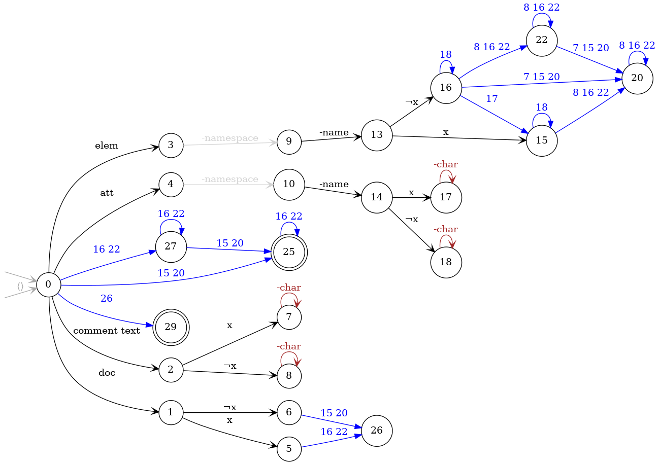
Figure 25: A schema for the intersection of xmldata model with ${{one^{x}}}$.

The results of our experiments are summarized in Table 26. For each automaton we present two numbers, size(#states), its size and the number of its states. Unless specified otherwise, we use a timeout of 1000 seconds whenever calling some determinization algorithm. Fields of the table are left blank if an exception was raised. This happens when the determinization algorithm reached the timeout, the memory was filled, or the stack overflowed. We conducted all the experiments on a Dell laptop with the following specs: Intel® Core™ i7-10875H CPU @ 2.30 GHz,16 cores, and 32 GB of RAM.

The first column $A$ of Table 26 reports on the Shas obtained from the queries Qn.m, by the compiler from [Sakho] that is written in XSLT. The second column $det(A)$ is obtained from Sha $A$ by accessible determinization. The blank cell in column $det(A)$ for query Q4.4 was raised by a timeout of the determinization algorithm. As one can see, this happens for all larger pairs ($n,m$). Furthermore, it appears that the sizes of the automata $det(A)$ grow exponentially with $n+m$.

In the third column $det(A\times S)$, the determinization of the product is presented. It yields much smaller automata than with $det(A)$. For Q4.3 for instance, $det(A)$ has size 53550 (2161) while $det(A\times S)$ has size 5412 (438). The computation continues successfully until Q6.4. For the larger queries Q6.5 and Q6.6, our determinizer runs out of memory. The fourth column $\mathit{det}_{S}(A)$ reports on schema-based determinization. For Q4.3 for instance we obtain 3534 (329). Here and in all given examples, both measures are always smaller for $\mathit{det}_{S}(A)$ than for $det(A\times S)$. While this may not always be the case, but both approaches yield decent results generally. The numbers for the $\mathit{det}_{S}(A)$ for Q6.6 are marked in gray, since its computation took around one hour, so we obtain it only when ignoring the timeout. In contrast to $det(A\times S)$, however, the computation of $\mathit{det}_{S}(A)$ did not run out of memory though. The fifth column $\mathit{scl}_{S}(\det(A))$ contains the schema-based cleaning of $\det(A)$. This automaton is equal to $\mathit{det}_{S}(A)$ by Correctness Theorem 23. Nevertheless, this cell is left blank in all but the smallest case $Q2.1$, since our datalog implementation of schema-based cleaning quickly runs out of memory for automata with many states. The time in seconds that for determinization in $det(A\times S)$ and $\mathit{det}_{S}(A)$ grows in dependence of the size of the output from 0.9 seconds until passing over the timeout.

In the last two columns for $mini(det(A\times S))$ and $mini(detS(A))$ we report the sizes of the minimization of $det(A\times S))$ and $\mathit{det}_{S}(A)$. It turns out that $mini(\mathit{det}_{S}(A))$ is always smaller than $mini(det(A\times S))$, if both can be computed successfully. An example of $mini(\mathit{det}_{S}(Q3.4))$ is shown in Figure 28.

	$A$	$det(A)$	$det(A\times S)$	$\mathit{det}_{S}(A)$	$\mathit{scl}_{S}($	$mini(det$	$mini($
					$det(A))$	$(A\times S))$	$\mathit{det}_{S}(A))$
Q2.1	166 (67)	1380 (101)	540 (92)	284 (53)	284 (53)	160 (43)	73 (20)
Q2.2	199 (79)	3635 (214)	1488 (167)	830 (106)		162 (43)	75 (20)
Q2.3	232 (91)	9574 (471)	4174 (334)	2424 (227)		164 (43)	77 (20)
Q2.4	265 (103)	24813 (1052)	11502 (713)	6826 (504)		166 (43)	79 (20)
Q4.1	240 (95)	8020 (435)	710 (116)	418 (75)		164 (43)	77 (20)
Q4.2	287 (111)	20945 (968)	1944 (215)	1220 (152)		166 (43)	79 (20)
Q4.3	334 (127)	53550 (2161)	5412 (438)	3534 (329)		168 (43)	81 (20)
Q4.4	381 (143)		14794 (945)	9856 (734)		170 (43)	83 (20)
Q6.1	314 (123)	48212 (2113)	880 (140)	552 (97)		168 (43)	81 (20)
Q6.2	375 (143)		2400 (263)	1610 (198)		170 (43)	83 (20)
Q6.3	436 (163)		6650 (542)	4644 (431)		172 (43)	85 (20)
Q6.4	497 (183)		18086 (1177)	12886 (964)			87 (20)
Q6.5	558 (203)			34376 (2169)
Q6.6	619 (223)			88666 (4862)

Figure 26: Statistics of automata for XPath queries: size(#states)

	$det(A\times S)$	$time(det(A\times S))$	$\mathit{det}_{S}(A)$	$time(\mathit{det}_{S}(A))$
Q2.1	540 (92)	1.4	284 (53)	0.9
Q2.2	1488 (167)	3.1	830 (106)	1.5
Q2.3	4174 (334)	11.1	2424 (227)	3.9
Q2.4	11502 (713)	54.5	6826 (504)	16.9
Q3.1	625 (104)	1.6	351 (64)	1.1
Q3.2	1716 (191)	4.1	1025 (129)	1.9
Q3.3	4793 (386)	16.9	2979 (278)	6.2
Q3.4	13148 (829)	84.9	8341 (619)	30.6
Q4.1	710 (116)	1.9	418 (75)	1.3
Q4.2	1944 (215)	5.5	1220 (152)	2.7
Q4.3	5412 (438)	22.9	3534 (329)	9.3
Q4.4	14794 (945)	120	9856 (734)	46.5
Q5.1	795 (128)	2.2	485 (86)	1.5
Q5.2	2172 (239)	7.1	1415 (175)	3.3
Q5.3	6031 (490)	32.2	4089 (380)	13
Q5.4	16440 (1061)	174.6	11371 (849)	71.7
Q6.1	880 (140)	2.8	552 (97)	1.6
Q6.2	2400 (263)	9.2	1610 (198)	4.6
Q6.3	6650 (542)	44.33	4644 (431)	19
Q6.4	18086 (1177)	231.8	12886 (964)	101.4
Q6.5			34376 (2169)	569.7
Q6.6			88666 (4862)	3284.5

Figure 27: Timings in seconds for the determinization of the schema product and for schema-based determinization.

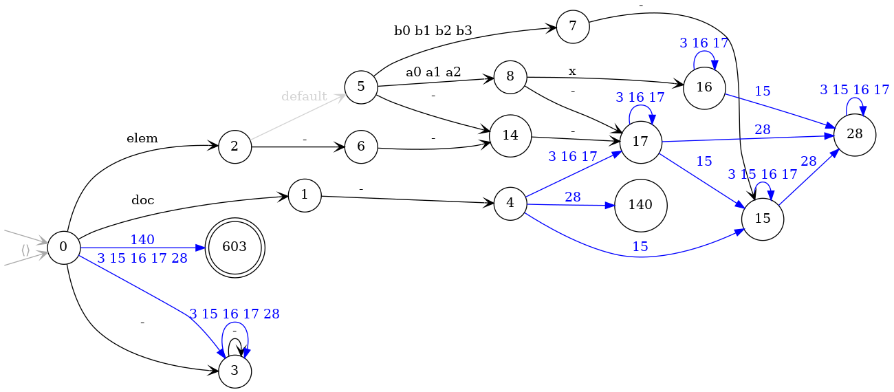
Figure 28: The automaton $mini(\mathit{det}_{S}(A))$ of the query Q3.4.

Figure 29: The automaton $mini(det(A\times S))$ of the query Q3.4.

Conclusion and Future Work

We presented an algorithm for schema-based determinization for Shas and proved that it always produces the same results as determinization followed by schema-based cleaning. We argued why schema-based determinization is often way more efficient than standard determinization, and why it is close in efficiency to the determinization of the schema-product. The statements are supported by upper complexity bounds and experimental evidence. The experimental results of the present paper are enhanced by follow up work [alserhalibench]. They show that one can indeed obtain small deterministic automata based on schema-based determinization of stepwise hedge automata for all regular XPath queries in practice. We hope that these automata are useful in the future for experiments with query answering.

References

[1]
[2]
Antonio Al Serhali &
Joachim Niehren
(2022): A Benchmark Collection of
Deterministic Automata for XPath Queries.
In: XML Prague 2022,
Prague, Czech Republic.
Available at https://hal.inria.fr/hal-03527888.
[3]
Rajeev Alur (2007):
Marrying Words and Trees.
In: 26th ACM SIGMOD-SIGACT-SIGART
Symposium on Principles of Database Systems,
ACM-Press, pp. 233–242.
Available at http://dx.doi.org/10.1145/1265530.1265564.
[4]
Rajeev Alur &
P. Madhusudan
(2004): Visibly pushdown languages.
In László Babai, editor: Proceedings of the
36th Annual ACM Symposium on Theory of Computing, Chicago, IL, USA, June
13-16, 2004, ACM, pp. 202–211,
10.1145/1007352.1007390.
[6]
Mikolaj Bojanczyk &
Igor Walukiewicz
(2008): Forest algebras.
In Jörg Flum,
Erich Grädel &
Thomas Wilke, editors: Logic and Automata: History and Perspectives [in Honor of
Wolfgang Thomas], Texts in Logic and
Games 2, Amsterdam University Press,
pp. 107–132.
[7]
Burchard von Braunm\IeCühl &
Rutger Verbeek
(1985): Input Driven Languages are
Recognized in log n Space.
In Marek Karplnski &
Jan van Leeuwen, editors:
Topics in the Theory of Computation,
North-Holland Mathematics Studies
102, North-Holland, pp.
1 – 19, 10.1016/S0304-0208(08)73072-X.
[9]
Julien Carme,
Joachim Niehren &
Marc Tommasi
(2004): Querying Unranked Trees with
Stepwise Tree Automata.
In Vincent van Oostrom,
editor: Rewriting Techniques and Applications,
15th International Conference, RTA 2004, Aachen, Germany, June 3-5, 2004,
Proceedings, Lecture Notes in Computer Science
3091, Springer, pp.
105–118, 10.1007/978-3-540-25979-4_8.
[10]
Hubert Comon, Max
Dauchet, Rémi Gilleron, Christof Löding, Florent Jacquemard, Denis Lugiez, Sophie Tison
& Marc Tommasi
(2007): Tree Automata Techniques and
Applications.
Available online since 1997:
http://tata.gforge.inria.fr.
[11]
Denis Debarbieux,
Olivier Gauwin,
Joachim Niehren,
Tom Sebastian &
Mohamed Zergaoui
(2015): Early nested word automata for
XPath query answering on XML streams.
Theor. Comput. Sci.
578, pp. 100–125,
10.1016/j.tcs.2015.01.017.
[12]
Martin Dietzfelbinger,
Anna R. Karlin,
Kurt Mehlhorn,
Friedhelm Meyer auf der Heide,
Hans Rohnert &
Robert Endre Tarjan
(1994): Dynamic Perfect Hashing: Upper
and Lower Bounds.
SIAM J. Comput.
23(4), pp. 738–761,
10.1137/S0097539791194094.
[14]
Olivier Gauwin,
Joachim Niehren &
Yves Roos (2008):
Streaming Tree Automata.
Information Processing Letters
109(1), pp. 13–17,
10.1016/j.ipl.2008.08.002.
[15]
Olivier Gauwin,
Joachim Niehren &
Sophie Tison
(2009): Earliest Query Answering for
Deterministic Nested Word Automata.
In: 17th International Symposium on
Fundamentals of Computer Theory, Lecture Notes
in Computer Science 5699, Springer
Verlag, pp. 121–132, 10.1007/978-3-642-03409-1_12.
[17]
Kurt Mehlhorn
(1980): Pebbling Moutain Ranges and its
Application of DCFL-Recognition.
In J. W. de Bakker &
Jan van Leeuwen, editors:
Automata, Languages and Programming, 7th
Colloquium, Noordweijkerhout, The Netherlands, July 14-18, 1980,
Proceedings, Lecture Notes in Computer
Science 85, Springer, pp.
422–435, 10.1007/3-540-10003-2_89.
[18]
Barzan Mozafari,
Kai Zeng & Carlo
Zaniolo (2012):
High-performance complex event processing over XML
streams.
In K. Selçuk Candan,
Yi Chen,
Richard T. Snodgrass,
Luis Gravano,
Ariel Fuxman,
K. Selçuk Candan,
Yi Chen,
Richard T. Snodgrass,
Luis Gravano &
Ariel Fuxman, editors: SIGMOD Conference, ACM, pp.
253–264, 10.1145/2213836.2213866.
[19]
Andreas Neumann &
Helmut Seidl
(1998): Locating Matches of Tree
Patterns in Forests.
In: Foundations of Software Technology
and Theoretical Computer Science, Lecture Notes
in Computer Science 1530, Springer
Verlag, pp. 134–145, 10.1007/978-3-642-03409-1_12.
[20]
Joachim Niehren &
Momar Sakho
(2021): Determinization and
Minimization of Automata for Nested Words Revisited.
Algorithms
14(3), p. 68,
10.3390/a14030068.
[21]
Joachim Niehren,
Momar Sakho &
Antonio Al Serhali
(2022): Schema-Based Automata