Tailoring microcombs with inverse-designed, meta-dispersion microresonators

Nonlinear-wave mixing in optical microresonators offers new perspectives to generate compact optical-frequency microcombs, which enable an ever-growing number of applications. Microcombs exhibit a spectral profile that is primarily determined by their microresonator’s dispersion; an example is the $\operatorname{sech}^{2}$ spectrum of dissipative Kerr solitons under anomalous group-velocity dispersion. Here, we introduce an inverse-design approach to spectrally shape microcombs, by optimizing an arbitrary meta-dispersion in a resonator. By incorporating the system’s governing equation into a genetic algorithm, we are able to efficiently identify a dispersion profile that produces a microcomb closely matching a user-defined target spectrum, such as spectrally-flat combs or near-Gaussian pulses. We show a concrete implementation of these intricate optimized dispersion profiles, using selective bidirectional-mode hybridization in photonic-crystal resonators. Moreover, we fabricate and explore several microcomb generators with such flexible ‘meta’ dispersion control. Their dispersion is not only controlled by the waveguide composing the resonator, but also by a corrugation inside the resonator, which geometrically controls the spectral distribution of the bidirectional coupling in the resonator. This approach provides programmable mode-by-mode frequency splitting and thus greatly increases the design space for controlling the nonlinear dynamics of optical states such as Kerr solitons.

Figure 1: Concept of microcomb inverse-design via meta-dispersion engineering

Microcombs — optical-frequency combs generated in driven Kerr resonators ¹ — are versatile light sources that offer unique properties for applications and integration of frequency-comb systems on a chip. Through experimentation and advances in the fabrication of integrated resonators, microcombs have progressed from a theoretical framework for Kerr-nonlinear optics ^{2, 3} to the generation of octave spanning combs for accurate and precise optical metrology ⁴. The large mode spacing and spectral width of microcombs have already found applications in parallel coherent communication ⁵ distance measurement ^{6, 7, 8}, and phase stabilization ⁹ for photonic-integrated frequency synthesis ⁴.

Microcomb generation often involves the formation of dissipative Kerr solitons (DKS) ^{10, 11}, which exist by balancing losses through nonlinear gain, anomalous group velocity dispersion (GVD), and pump laser detuning, through nonlinear phase shifts. Dominated by second-order dispersion, the resulting DKS pulses feature a squared secant hyperbolic profile in time and frequency domain; see fig. 1. Owing to this equilibrium with the Kerr-nonlinearity, the dispersion of the resonator – or more generally mode-by-mode frequency mismatch from the resonator’s free-spectral range (FSR) – primarily determines the pulse shape and spectrum of nonlinear states it supports.

Tailoring the comb spectral profile is desired in applications like telecommunications where high power per mode and spectral flatness improve the performance and efficiency of data links. However, there is currently no direct relationship connecting the desired microcomb spectrum with the required dispersion, material properties, or physical geometry of the resonator. Additionally, achieving precise dispersion control in resonators has historically been a significant challenge, lacking a demonstrated technique for imparting arbitrary dispersion properties. Nevertheless, recent advancements in numerical computation and machine learning have introduced new capabilities and tools for system design and optimization ^{12, 13, 14, 15}. Integrated photonics, on the other hand, not only offers potential for miniaturization of large-scale systems but also enables greater control over guided modes of light, particularly in photonic crystals ¹⁶, or topology-optimized elements ^{17, 18} which paved the way for highly customizable inverse-designed microresonators ¹⁹

Here, we propose and implement an inverse-design process to shape the spectral envelope of microcombs. Our approach numerically optimizes an arbitrary dispersion profile to tailor the associated nonlinear state of the resonator toward a target pulse shape and spectrum. The resulting complex dispersion relation is then implemented indirectly by means of Photonic Crystal Resonators (PhCRs), where the resonance frequencies can be controlled via multiple selective mode splitting ^{20, 21, 5} to create a meta-dispersion (fig. 1). We demonstrate a full iteration of the design process and first experimental evidence of microcomb shaping. The design steps followed in our work are summarised in fig. 1. First, we numerically solve the governing equation of the resonator, and use a genetic algorithm (GA) to iteratively optimize the dispersion and pumping parameters to create a desired microcomb shape. While a similar GA-based method was concurrently developed ²³, our approach notably introduces an analytical model based on the target comb’s Kerr shift to efficiently generate an initial dispersion. Second, we determine the PhCR topology needed to achieve the optimized dispersion. Finally, we demonstrate realizations of meta-dispersion in PhCR microresonators and initial observations of comb generation in these devices.

Results

Inverse-design dispersion optimization

We first describe our precise formalism and notation. The Lugiato–Lefever equation ² (LLE) accurately models the driven nonlinear resonator and can be written as a set of coupled mode equations in the spectral domain:

$$\frac{\partial\tilde{A}_{\mu}}{\partial t} =-\left[\dfrac{\kappa}{2}+i\,\left(\delta\omega-D_{\rm int}(\mu)\right)\right]\tilde{A}_{\mu}$$ (1)

$$+i\,g_{0}\,\mathcal{F}\left[\left|A\right|^{2}A\right]_{\mu}+\sqrt{\kappa_{\rm ex}\,\dfrac{P_{\rm in}}{\hbar\omega_{0}}}\,\delta_{\mu=0}$$

where $\mu$ is the azimuthal mode number relative to the pumped mode, $\left|\tilde{A}_{\mu}(t)\right|^{2}$ is the number of photons in mode $\mu$ as a function of the ‘slow’ time $t$, $P_{\rm in}$ and $\delta\omega=\omega_{0}-\omega_{\rm pump}$ are respectively the pump power and detuning terms ¹¹ (the detuning is positive if the laser frequency is lower than the resonance frequency), $\kappa$ is the resonator FWHM linewidth, and $\kappa_{\rm ex}$ is the coupling rate. $\mathcal{F}\left[\cdot\right]_{\mu}$ represents the Fourier series operator and $g_{0}$ the per photon Kerr shift of the resonator modes. $P_{\rm th}=\hbar\omega_{0}\kappa^{3}/8g_{0}\kappa_{\rm ex}$ is the threshold pump power for initial four-wave mixing in resonators and is useful to rescale the power quantities. The operator $D_{\rm int}(\mu)=(\omega_{\mu}-\omega_{0})-D_{1}\,\mu$ represents the resonator dispersion ²⁴ and measures the deviation of the resonance frequencies from an equidistant FSR $D_{1}$.

Optimization problem

The dispersion plays a key role in determining the temporal and spectral shape of localized structures emerging from nonlinear effects in a resonator. One problem of interest is to find the dispersion $D_{\rm int}$ of the resonator that yields a comb with desired properties, and is a steady-state solution of the LLE; see fig. 1.

To simplify the problem, we describe the dispersion using a set of polynomial coefficients $D_{k}$ such that $D_{\rm int}(\mu)=\sum_{k=2}^{8}\frac{D_{k}}{k!}\mu^{k}+\frac{\gamma_{0}}{2}\,\delta_{\mu=0}\;.$ The extra degree of freedom $\gamma_{0}$ corresponds to a discrete shift in the frequency of the pump mode, which is known to favour the formation of pulses, notably in the normal dispersion regime ^{25, 20, 26}. An additional constraint limits the pump power within a specified budget of $P_{\rm max}$. Our objective is to determine the values of $D_{k}$, $\gamma_{0}$, $\delta\omega$, and $P_{\rm in}$ that result in a stationary comb profile that best satisfies our objective, as quantified by the error function $\mathcal{E}(\tilde{A}\mu)$ (see the Methods section for details). To solve this optimization problem, we use a genetic evolutionary algorithm ^{27, 28, 23}.

Initialization

It is useful to leverage prior knowledge to initialize the problem as close as possible to a potential solution. An initial dispersion profile is first derived based on a simple heuristic, inspired by the essential principle of the soliton balance of dispersion by the Kerr shift. Thus, in the frequency domain, the dispersion $D_{\rm int}^{\rm initial}(\mu)$ is initialized as the opposite of the Kerr spectral shift $\delta^{\rm Kerr}_{\mu}$ of the target comb state $\tilde{A}^{\rm target}_{\mu}$, according to ²⁰

$$D_{\rm int}^{\rm init}(\mu)=-\delta^{\rm Kerr}_{\mu}=-\Re\left(\dfrac{\mathcal{F}\left[\left|A^{\rm target}\right|^{2}\,A^{\rm target}\right]_{\mu}}{\tilde{A}^{\rm target}_{\mu}}\right)$$ (2)

Hence this relation is fitted with a polynomial to obtain the initial dispersion coefficients. The pump laser parameters ($P_{\rm in}$, $\delta\omega$) are also initialized, below $P_{\rm max}$ for the former, and based on the maximum single-mode Kerr-shift for the latter ²⁹. A population of dispersion candidates, with a typical size of $N_{\rm pop}=208$, is then generated from random variations around these initial parameters.

Figure 2: Dispersion optimization for comb shaping 2 Flowchart of the evolutionary algorithm used to optimize the dispersion and driving parameters to match a given comb spectral profile.

Figure 3: Meta-dispersion in PhCR

Figure 4: Examples of meta-dispersion in PhCR

Figure 5: Comb generation in meta-dispersion PhCR

Evolution step

The GA loop for finding the optimal parameters consists of two steps, presented in fig. 2. First, the steady-state intra-resonator field is computed for each member of the population by integrating the LLE equation via split-step Fourier transform. Next, the steady-state comb solutions are ranked based on an error function $\mathcal{E}(\tilde{A}_{\mu})$ that measures their fitness for the optimization goal. This metric can be the mean square error to a target comb shape or a binary criterion that checks whether a given power target is reached for certain lines. To ensure stable and low noise combs, highly fluctuating states are penalized. If a solution meets a fitness threshold or a maximum generation number is reached, the algorithm stops. Otherwise, a new population is created by combining two parents’ dispersion coefficients (crossover) and adding a random variation (mutation) to generate each new candidate, before the loop continues. The GA is further detailed in the Methods section.

Optimization results

First, we show how the dispersion can be optimized to obtain a comb with nearly Gaussian spectral profile in the resonator. Figure 2 shows the target comb, the initial comb and the result after optimization. The initial dispersion profile, shown in fig. 2, is calculated from the target comb Kerr shift using eq. 6. The optimized dispersion appears almost identical to this initial profile. The GA mainly modified the pumping conditions to fit the spectral width to the target.

For applications, such as telecommunications, a flat microcomb with high conversion efficiency and maximum power per line is typically required. Using a rectangular comb target is problematic as the function is discontinuous. A raised-cosine shape makes a more realistic target for optimization as it has a smoother decay outside the bandwidth of interest, as shown in fig. 2. Moreover, the regularity of the function makes it possible to compute the Kerr shift, which again provides an excellent starting point (see fig. 2). The GA mainly modifies the pump mode shift $\gamma_{0}$ and the driving parameters. These examples demonstrate that our method can perform a ‘fitting’ of a specific comb target by changing the parameters of the LLE. Our initialization technique also proves to be very effective in coarsely matching a desired comb shape, which can speed up the convergence of the GA, especially if it preferentially adjusts the pumping parameters. An exhaustive search could even be conducted.

An alternative approach to obtain efficient flat comb generation, is to modify the fitness metric to enforce a comb line power of at least $P_{\rm min}$ over a given bandwidth (see methods). We initialize the dispersion from the Kerr shift of a flat-top comb model (see the method section), which does not satisfy the power criterion, although we sought to obtain the highest possible power. After the optimization, the power criterion is met by the resulting comb, as shown in fig. 2. Interestingly, the associated dispersion profile, shown in fig. 2, is dominantly normal for higher relative mode number, and turns locally anomalous near the pump mode. The general comb shape resembles the typical ‘platicon’ spectrum obtained in normal dispersion ^{32, 25, 26}, i.e. a strong central lobe surrounded by two pronounced wings, which is known to have high conversion efficiency ³³. However, the center lobe here has a flattened $\operatorname{sech}$-like profile ¹¹. In this optimization problem, where the target comb is not provided, the GA plays a prominent role since it extensively explores the parameter space and converge to a radically different solution from the initialization. Overall, the heuristic approach and the GA are complementary tools in the inverse-design process. The former can be used to quickly obtain a rough estimate of the optimal parameters in specific problems, while the latter can refine the parameters and explore a broader range of solutions. Finally, it should be noted that the algorithm does not guarantee to find a global optimum to the problem. However, we tested the convergence robustness by repeating this optimization problem three times, and obtained similar dispersion profiles for all iterations.

An additional scenario, targeting enhanced dispersive-wave emission is discussed in the supplementary information (SI). Before finalizing the meta-dispersion design, bidirectional LLE simulations ³⁴ are performed, with sweeps of $\delta\omega$, $P_{\rm in}$ and $\gamma_{0}$ to ensure that the desired nonlinear state can be achieved in the resonator, under realistic driving conditions (see the SI for details).

Meta-dispersion

The complex dispersion obtained with the GA is realized by means of engineered mode splittings in a PhCR (see fig. 1). A distributed corrugated grating is fabricated on the inner wall of a ring resonator, introducing a clockwise – counterclockwise coupling and hence a mode hybridization. The corrugation’s period and amplitude respectively control the impacted longitudinal mode and the splitting amplitude. By appropriately superposing multiple corrugations, we generalize this concept to simultaneously control multiple dozens of modes, while faithfully retaining a designed spectral distribution of mode splitting $\gamma_{\mu}$. The combined ring waveguide dispersion and mode splitting distribution define an effective synthetic dispersion, or meta-dispersion, on the blue and red shifted branches corresponding to the up- and down-frequency-shifted split modes.

PhCR design

Figure 3 shows the implementation of the optimization result using meta-dispersion. The dispersion is decomposed into two components. First, the ring’s dispersion is chosen to match the general sign of the optimized dispersion at high mode numbers, which allows us to set the waveguide’s cross-section. The mode splitting spectral distribution $\gamma_{\mu}$ near the central modes is then taken as twice the difference between the target dispersion and that of the waveguide, so that one of the shifted branches coincides with the target dispersion. Finally, the corrugation’s azimuthal profile $\rho(\phi)$ is calculated by use of Fourier synthesis of this distribution:

$$\rho(\phi)=\sum_{\mu\in\mathbb{Z}}\frac{\tilde{\rho}_{\mu}}{2}\,\cos\left(2(m_{0}+\mu)\,\phi+\xi\mu^{2}\right),$$ (3)

where the modulation amplitude $\tilde{\rho}_{\mu}$ is determined based on an experimental calibration of the frequency splitting vs PhC amplitude relation $\gamma(\rho)$ (see methods). $m_{0}$ is the ‘carrier’ modulation which sets the azimuthal mode index of the central mode $\mu=0$.

Importantly, the various frequency components of the grating are superposed with a phase offset (chirp $\xi$) to distribute the corrugation’s amplitude evenly across the ring perimeter. This minimizes the corrugation peak amplitude and preserves the shape of the desired splitting distribution. Indeed, since we use the fundamental transverse electric mode of the waveguide, which has the highest Q factor, the relationship $\gamma(\rho)$ is non-monotonic. A similar dispersion control approach was developed concurrently in ref. ⁵, using the transverse magnetic mode, for which $\gamma(\rho)$ is monotonic.

Characterization

We fabricate the designed devices in a 570 nm-thick Ta2O5 (tantala) layer on thermal silicon oxide, without top-cladding (see ³⁵ for fabrication details). The ring resonator baseline dispersion is controlled by changing the width of the waveguide (rw). The resonator FSR are selected as 200 or 400 GHz. Figure 3 shows a scanning electron microscope (SEM) image of a completed PhCR, revealing the corrugation pattern.

The dispersion and quality factors are characterized by use of a scanning laser spectroscopy method ³⁶, and the resonances frequencies are detected and the integrated dispersion $D_{\rm int}$ is retrieved. We first perform a meta-dispersion demonstration with a Gaussian splitting profile in a normal dispersion ring, shown in fig. 3. The integrated dispersion $D_{\rm int}$ illustrates the deviation of each frequency splitting branch from the continuous resonator dispersion. The resonance pair for each longitudinal split mode is fit with a model to recover the characteristics of the resonances. Thus, we found that adding the corrugation does not degrade the quality factor for modulation depths under $10\text{\,}\mathrm{\char 37\relax}$ of the ring width. The splitting spectral profile $\gamma_{\mu}$ is also retrieved and shows a Gaussian shape in excellent agreement with the design.

This characterization is repeated for several resonators, in which only the zeroth mode splitting is changed. Their respective splitting distribution is reported in fig. 3, which shows first the excellent reproduction of the global Gaussian profile across the devices. Second, we observe that single mode splitting control is accurately retained, in spite of splitting multiple tens of adjacent modes.

Figure 4 shows further examples of meta-dispersion demonstrations, with various configurations of base ring dispersion (normal and anomalous) and to tailor the dispersion of the red- or blue-shifted branch. The principle works remarkably well in all cases, such as flattening the blue-shifted branch or carve a localized stronger dispersion. Deviations from the measured profiles are nevertheless observed, which are caused by avoided mode crossing. These are due to the presence of higher order modes in the resonator and can be problematic for the formation of DKS ³⁷.

Comb generation

We conducted comb generation experiments in PhCR structures with meta-dispersion profiles for two configurations of target comb spectra. To initiate comb generation, the laser power is increased, and its frequency is swept through the red-shifted resonance of the split mode $\mu=0$, starting from the center of the split and increasing the laser wavelength.

The first configuration, targets a comb with a minimum comb line power. The measured dispersion, shown in fig. 5, corresponds to that of a normal-dispersion ring resonator ($\text{rw}=$2.3\text{\,}\mathrm{\SIUnitSymbolMicro m}$$, radius $109\text{\,}\mathrm{\SIUnitSymbolMicro m}$) with a slight anomalous meta-dispersion near the pump, to reproduce the optimized design shown in fig. 2. The device was pumped with $55\text{\,}\mathrm{mW}$ on-chip. The detuning was first increased to trigger the formation of an initial comb state and then reduced (backward tuning), to induce switching into the state shown in fig. 5. The spectrum is analogous to a platicon comb ²⁵, but with a flattened center lobe, compared to a single PhC device (shown in red in fig. 5), and a wider bandwidth for the same pump power and base ring dispersion. The number of consecutive teeth within the 5-dB bandwidth is increased from $\sim 20$ to $\sim 50$. Notably, the power per line in the central lobe is lower than in the wings, as featured in the predicted inverse-design comb in fig. 2. We confirmed that this comb is a low-noise state, by recording its intensity noise, which coincides with the instrument’s noise floor (fig. 5). Several comb state transitions and breathing stages were observed by changing the power and detuning (see SI), revealing complex dynamics.

The second configuration aims at generating Gaussian-shaped combs. The ring features anomalous base dispersion ($\text{rw}=$1.55\text{\,}\mathrm{\SIUnitSymbolMicro m}$$, radius $53\text{\,}\mathrm{\SIUnitSymbolMicro m}$), and the meta-dispersion is chosen to replicate the computed optimized dispersion in fig. 2 over a limited range of the red-shifted branch, as shown in fig. 5. This meta-dispersion PhCR device is compared to a regular ring resonator with the same geometry to provide a baseline for comparison. Figure 5 shows the combs produced in each resonator in the unstable modulation instability (MI) regime, when pumping with $\sim 90\text{\,}\mathrm{mW}$ on-chip. We also ensured that the comb states have comparable intensity noise properties and are in the same stage of MI (subcomb merging ³⁸). The regular ring produces a typical MI comb, with powerful comb lines surrounding the pump (corresponding to primary lines) and a dip in comb line power near the pump. The meta-dispersion resonator exhibits a markedly different comb envelope, with a smoother decrease in power from pump to wings. The MI comb bandwidth is also largely reduced, highlighting the impact of the PhCR in shaping the microcomb. Unfortunately, stable mode-locked soliton sates ³⁸ could not be obtained in this meta-dispersion device, nor in the regular ring, likely due to the photothermal effect in the cavity ^{39, 40}, which is particularly strong in Ta2O5. The presence of an avoided mode crossing near the pumped mode can also hinder soliton formation ³⁷. Therefore, the PhCR comb envelope does not match the expected Gaussian shape, which is obtained in the soliton state, as shown below. Nevertheless, we believe that these limitations are not fundamental, but of technical nature, and that the desired states can be achieved on a more mature technology platform.

Comb simulation

We have compared these experimental observations with bidirectional LLE simulations ³⁴, detailed in the SI.

First, we set out to reproduce the comb states in noisy MI, in order to validate our model. The parameters used are taken from the experimental measurements of the resonators shown in fig. 5. The detuning is the only adjusted parameter, to recover the unstable modulation instability regime in each resonator. The averaged spectra shown in fig. 6 are in good agreement with our experimental observations.

Figure 6: Numerical simulation of comb states

Second, since numerical simulations are not subject to thermal effects, they allow us to extrapolate the shape of the stationary ‘mode locked’ pulsed states in each resonator, which are reached at higher detuning (see SI). The corresponding comb spectra are overlaid in fig. 6. The PhCR comb clearly deviates from the usual DKS $\operatorname{sech}^{2}$ profile formed in the standard resonator, and follows a Gaussian shape within the meta-dispersion bandwidth. These projections further show that the nonlinear cavity field state is governed by the meta-dispersion.

The results presented here show only the combs co-propagating with the pump. Since the combs are supported by hybrid modes, whose splitting amplitude is significantly larger than the Kerr shift ^{20, 26}, they are typically generated with near equal power in the clockwise and counterclockwise direction. However, transitions to a dominant direction have been observed, especially when the dispersion is predominantly normal.

Discussion

In summary, we have demonstrated the spectral shaping of microcombs by inverse design, using an optimization layer on the LLE, and we have demonstrated the scalable use of PhCRs for effective meta-dispersion engineering. This flexible approach enables mode-by-mode selectivity and control of nonlinear frequency shifts that are critical in Kerr microcombs. We also showed that meta-dispersion can be used in the nonlinear regime to perform spectral shaping of microcombs.

Further fundamental studies are still needed to fully understand the nonlinear dynamics in hybrid modes, to help control comb formation in these new devices, and to refine our inverse design approach. Moreover, we are considering several ways to enhance our method. The optimization algorithm could occur directly on the meta-dispersion parameters, using the bidirectional LLE within the evolution loop. This requires nonetheless a robust method of seeding the cavity field in both directions. In this respect, machine learning could contribute to speed up the computation, and robustly find the soliton or related nonlinear eigenstates. Other implementations of the optimised dispersion can be conceived, based on coupled resonator chains ^{41, 33}, through engineered avoided mode crossing with higher-order modes ⁴², or by using discrete inverse-designed reflectors ¹⁹.

We believe that our comb customization procedure is promising to fully unlock the application potential of microcombs. First, in optical telecommunications, where it can maximize the conversion efficiency and the power per line in the bandwidth of interest. In spectroscopy, our concept can help open access to new wavelength ranges, or shape combs that target specific chemical species. Additionally, one could try to optimize the control of the comb parameters (repetition frequency, offset), to improve its intrinsic stability. Finally, the presented method offers new avenues for nonlinear physics, making previously unrealistic dispersion profiles accessible, while contra-propagative coupling promises to produce a myriad of complex dynamics that remain to be explored.

Authors contributions

E.L. implemented the optimization algorithm, performed the experiments and analysed the data. E.L and S.-P.Y. contributed to the numerical simulations and resonators design. T.C.B. and D.R.C fabricated the microresonators. E.L. wrote the manuscript, with input from all authors. S.P. supervised the project.

Competing Interests

David R. Carlson is a cofounder of Octave Photonics. The remaining authors do not currently have a financial interest in Ta2O5-integrated photonics.

Methods

Genetic algorithm

Our goal is to find the parameters $D_{k},\gamma_{0},\delta\omega,P_{\rm in}$ that yield a stationary comb profile (for the LLE) $\tilde{A}_{\mu}$ that minimizes an error function $\mathcal{E}(\tilde{A}_{\mu})$, which quantifies our objective. The optimization problem can be formalized as follows:

$$\left[\begin{aligned} &\underset{D_{k},\gamma_{0},\delta\omega,P_{\rm in}}{\operatorname{minimize}}\;\mathcal{E}(\tilde{A}_{\mu})\\ &\text{subject to}\;\left\{\begin{aligned} &\text{\lx@cref{creftype~refnum}{eq:LLEeq}}=0\\ &P_{\rm in}\leq P_{\rm max}\end{aligned}\right.\end{aligned}\right.$$ (4)

The latter term contrains the pump power within a limited power budget. Based on the available power and our resonator’s properties, we set $P_{\max}=13\,P_{\rm th}$.

The LLE steady state field for each member of the population, is estimated using split step Fourier transform integration ² of eq. 1. An initial pulse consisting in an approximate soliton profile ³, is seeded in the simulation and its evolution through the LLE is computed for 100 photon lifetimes; the pump power and detuning are kept constant. Though the stationary state of the LLE can be found using a Newton–Raphson method ³, we found that its convergence was slower and less systematic than the split step approach, especially in complex dispersion profiles.

The steady-state solution of each member of the population is then ranked according to a metric $\mathcal{E}(\tilde{A},D_{k})$, which measures each comb’s ‘fitness’ with respect to the optimization goal. The smaller the error, the more fit the candidate. This metric can be the squared Euclidean distance to a target comb shape $\tilde{A}_{\mu}^{\rm target}$:

$$\mathcal{E}(\tilde{A})=\sum_{\mu\neq 0}\Bigl{(}|\tilde{A}_{\mu}|-|\tilde{A}_{\mu}^{\rm target}|\Bigr{)}^{2}$$ (5)

This metric can be complemented to favour stable low-noise states, by adding the standard deviation of the mean comb power, estimated during the second half of the split-step evolution.

The raised cosine comb spectrum shape is defined with the following expression:

$$\tilde{A}_{\mu}^{\rm target}=\begin{cases}1,&\frac{|\mu|}{\Delta}\leq(1-\beta)\\ \cos^{2}\left[{\frac{\pi}{4\beta}\left(\frac{|\mu|}{\Delta}-{(1-\beta)}\right)}\right],&\left|\frac{|\mu|}{\Delta}-1\right|\leq\beta\\ 0,&{\text{otherwise}}\end{cases}$$ (6)

where $\Delta$ is the comb’s 3-dB bandwidth and $\beta$ is the roll-off factor, which controls the slope of the power decay in the outer lines of the comb.

Another metric can be used to ensure a minimum comb line power $P_{\rm min}$ over a given bandwidth $\Delta$:

$$\mathcal{E}(\tilde{A})=\sum_{\mu\in\Delta}\max\left(0,\,P_{\rm min}-\dfrac{\hbar\omega_{\mu}\,D_{1}}{2\pi}\,|\tilde{A}_{\mu}|^{2}\right)$$ (7)

This way, comb lines exceeding the criterion are not penalized. A soft threshold function can also be used to force the power to be within a given range. The flat-top comb initial model follows the equation $A_{\mu}=A_{0}/(1+\mu/B)^{8}$, where $B$ sets the bandwidth and $A_{0}$ the comb line magnitude. $A_{0}$ was set to the maximum value authorizing convergence to a stable comb state.

In general, engineering the error function is a key aspect of inverse design problems, and it requires careful consideration of the optimization goals, constraints, and trade-offs. The two functions in eqs. 5 and 7 are two extreme cases when is come to evaluating the combs shape over a bandwidth of interest, as the former gives equal weights to all comb lines, while the latter only accounts for the lines within a spectral region and disregards the lines outside. A more general approach is to introduce weight factors that reflect the importance of certain comb lines or regions of the spectrum. Alternatively, one could also use a weighting function that assigns higher importance to certain dynamics of the comb, to identify phenomena such as breathing.

Note that if the targeted problem is frequency-symmetric with respect to the pump, all odd dispersion coefficients can be set to zero and the optimization can be performed only on the even terms, reducing the number of variables while ensuring the symmetry of the solution.

At each iteration of the GA loop, a new population is created. First the two best individuals from the last generation are carried over unchanged (elitism), which guarantees that the current optimum is preserved. Then, each new offspring is generated by selecting two (or more) parents at random, with a probability inversely proportional to their residual error, so that the fittest to the problem are selected more frequently (roulette wheel selection). The dispersion coefficients (genes) of the offspring are randomly selected from its parents (uniform crossover). The better the fitness of a parent, the more likely its genes will be selected. Finally, the offspring’s genes are mutated by adding a random value drawn using a normal distribution with standard deviation $\sigma$. As the number of generation increases, $\sigma$ is gradually decreased to favour the convergence of the algorithm.

Our genetic evolutionary algorithm was developed in MATLAB, without the use of existing optimization libraries. To speed up the steady-state intra-resonator field calculation, we implemented parallelization of the split-step Fourier transform computations. This allowed us to significantly reduce the computation time, making the optimization process feasible within a few hours.

Mode splitting calibration

The relation between PhC amplitude and mode splitting was calibrated experimentally on a series of single period PhCR with identical base geometry (ring radius $109.5\text{\,}\mathrm{\SIUnitSymbolMicro m}$, width $2\text{\,}\mathrm{\SIUnitSymbolMicro m}$, height $570\text{\,}\mathrm{nm}$), while the PhC amplitude $\rho_{\rm PhC}$ is swept. The results are shown in fig. S1. Note that the reported amplitude corresponds to the design value and not the measured geometry.

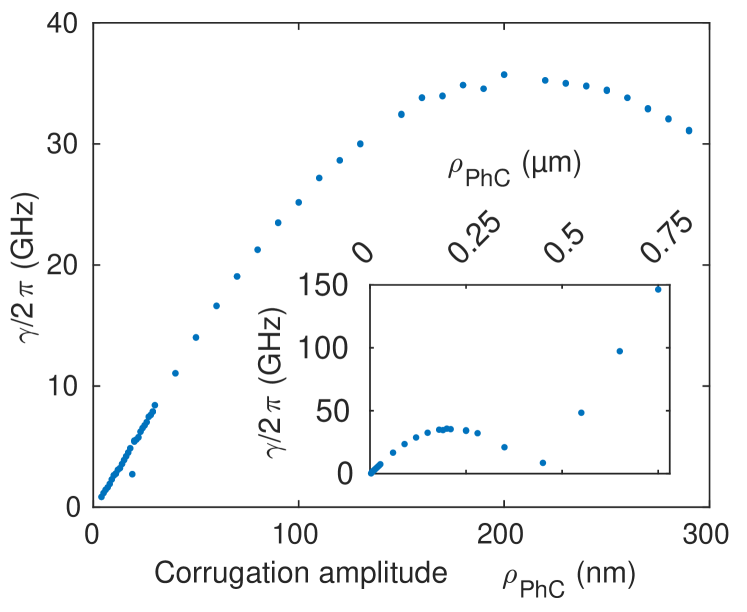
Extended Data Figure S1: PhC and mode splitting calibration. Measured mode splitting of the target mode as a function of corrugation amplitude $\rho_{\rm PhC}$ (single frequency PhC), measured across 114 resonators. The inset shown an extended range of $\rho_{\rm PhC}$.

While the relation is linear at small corrugation amplitudes, it reaches a maximum around $\rho_{\rm PhC}\sim$200\text{\,}\mathrm{nm}$$ for $\gamma/2\pi\sim$35\text{\,}\mathrm{GHz}$$ and the tuning direction reverses. We found that a near null splitting can be obtained for $\rho_{\rm PhC}\sim$420\text{\,}\mathrm{nm}$$, before $\gamma$ increases again for larger amplitude values (see inset of fig. S1). This counter-intuitive bandgap closing was observed and explained by Gnan et al. in photonic wire Bragg gratings and is related to Brewster angle incidence ⁴ and is also studied in ref. ⁵.

We did not observe any significant deviation from this calibration, upon splitting multiple modes. Chirping the frequency components of the corrugation, in order to reduce amplitude variations, allows us to stay within the linear segment of this relationship and ensures a good replication of the splitting profile, as shown in fig. S2. Limiting the amplitude variations in the corrugation also avoids the need for high aspect ratio etching, which thus simplifies the nanofabrication of the PhCR.

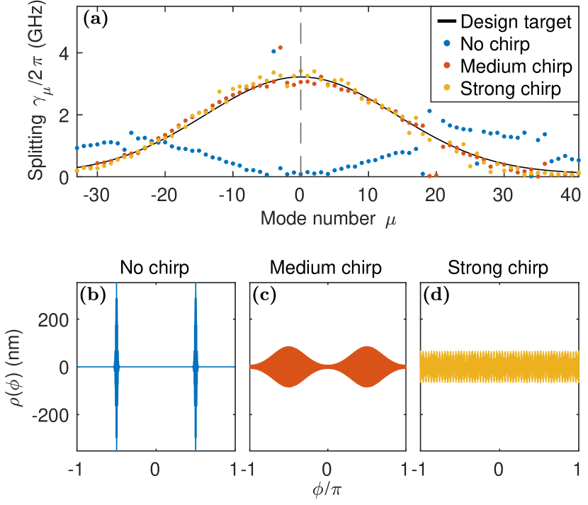
Extended Data Figure S2: Effect of distributing the PhC pattern along the ring perimeter. (a) Measured mode splitting distribution with various amount of chirping applied to the corrugation pattern. The design target is the Gaussian distribution shown in black. (b-c) Spatial profiles of the designed corrugations. (a) Without chirp, the splitting distribution is distorted and even inverted. The effect is avoided by chirping the pattern.

Data availability statement

The data and code used to produce the figures of this manuscript are available on Zenodo: https://doi.org/10.5281/zenodo.7998103.

Code availability statement

The code for the genetic algorithm implementation used to perform the dispersion optimization is available at: https://github.com/ErwanLucas/inverseLLE.

See pages - of SI.pdf

References

- 1 Kippenberg, T. J., Gaeta, A. L., Lipson, M. & Gorodetsky, M. L. Dissipative Kerr Solitons in Optical Microresonators. Science 361, eaan8083 (2018).
- 2 Lugiato, L. A. & Lefever, R. Spatial Dissipative Structures in Passive Optical Systems. Physical Review Letters 58, 2209–2211 (1987).
- 3 Coen, S., Randle, H. G., Sylvestre, T. & Erkintalo, M. Modeling of Octave-Spanning Kerr Frequency Combs Using a Generalized Mean-Field Lugiato-Lefever Model. Optics letters 38, 37–9 (2013).
- 4 Spencer, D. T. et al. An Optical-Frequency Synthesizer Using Integrated Photonics. Nature 557, 81–85 (2018).
- 5 Marin-Palomo, P. et al. Microresonator-Based Solitons for Massively Parallel Coherent Optical Communications. Nature 546, 274–279 (2017).
- 6 Trocha, P. et al. Ultrafast Optical Ranging Using Microresonator Soliton Frequency Combs. Science 359, 887–891. PMID: 29472477 (2018).
- 7 Suh, M.-G. & Vahala, K. J. Soliton Microcomb Range Measurement. Science 359, 884–887 (2018).
- 8 Riemensberger, J. et al. Massively Parallel Coherent Laser Ranging Using a Soliton Microcomb. Nature 581, 164–170 (2020).
- 9 Drake, T. E. et al. Terahertz-Rate Kerr-Microresonator Optical Clockwork. Physical Review X 9, 031023 (2019).
- 10 Leo, F. et al. Temporal Cavity Solitons in One-Dimensional Kerr Media as Bits in an All-Optical Buffer. Nature Photonics 4, 471–476 (2010).
- 11 Herr, T. et al. Temporal Solitons in Optical Microresonators. Nature Photonics 8, 145–152 (2013).
- 12 Lorenc, D., Velic, D., Markevitch, A. & Levis, R. Adaptive Femtosecond Pulse Shaping to Control Supercontinuum Generation in a Microstructure Fiber. Optics Communications 276, 288–292 (2007).
- 13 Sigmund, O. On the Usefulness of Non-Gradient Approaches in Topology Optimization. Structural and Multidisciplinary Optimization 43, 589–596 (2011).
- 14 Jensen, J. & Sigmund, O. Topology Optimization for Nano-Photonics. Laser & Photonics Reviews 5, 308–321 (2011).
- 15 Genty, G. et al. Machine Learning and Applications in Ultrafast Photonics. Nature Photonics 15, 91–101 (2021-02-30).
- 16 Joannopoulos, J. D., Villeneuve, P. R. & Fan, S. Photonic Crystals: Putting a New Twist on Light. Nature 386, 143–149 (1997).
- 17 Molesky, S. et al. Inverse Design in Nanophotonics. Nature Photonics 12, 659–670 (2018).
- 18 Yu, Z., Cui, H. & Sun, X. Genetically Optimized On-Chip Wideband Ultracompact Reflectors and Fabry–Perot Cavities. Photonics Research 5, B15 (2017).
- 19 Ahn, G. H. et al. Photonic Inverse Design of On-Chip Microresonators. ACS Photonics 9, 1875–1881 (2022).
- 20 Yu, S.-P. et al. Spontaneous Pulse Formation in Edgeless Photonic Crystal Resonators. Nature Photonics 15, 461–467 (2021).
- 21 Lu, X., Rao, A., Moille, G., Westly, D. A. & Srinivasan, K. Universal Frequency Engineering Tool for Microcavity Nonlinear Optics: Multiple Selective Mode Splitting of Whispering-Gallery Resonances. Photonics Research 8, 1676 (2020).
- 22 Moille, G., Lu, X., Stone, J., Westly, D. & Srinivasan, K. Fourier Synthesis Dispersion Engineering of Photonic Crystal Microrings for Broadband Frequency Combs. Communications Physics 6, 1–11 (2023).
- 23 Zhang, C., Kang, G., Wang, J., Pan, Y. & Qu, J. Inverse Design of Soliton Microcomb Based on Genetic Algorithm and Deep Learning. Optics Express 30, 44395–44407 (2022).
- 24 Brasch, V. et al. Photonic Chip–Based Optical Frequency Comb Using Soliton Cherenkov Radiation. Science 351, 357–360 (2016).
- 25 Lobanov, V. E., Lihachev, G., Kippenberg, T. J. & Gorodetsky, M. Frequency Combs and Platicons in Optical Microresonators with Normal GVD. Optics Express 23, 7713 (2015).
- 26 Yu, S.-P., Lucas, E., Zang, J. & Papp, S. B. A Continuum of Bright and Dark-Pulse States in a Photonic-Crystal Resonator. Nature Communications 13, 3134 (2022).
- 27 Holland, J. H. Adaptation in Natural and Artificial Systems: An Introductory Analysis with Applications to Biology, Control, and Artificial Intelligence (1992).
- 28 Kumar, M., Husain, M., Upreti, N. & Gupta, D. Genetic Algorithm: Review and Application. SSRN Electronic Journal (2010).
- 29 Coen, S. & Erkintalo, M. Universal Scaling Laws of Kerr Frequency Combs. Optics letters 38, 1790–2 (2013).
- 30 Fan, S. Sharp Asymmetric Line Shapes in Side-Coupled Waveguide-Cavity Systems. Applied Physics Letters 80, 908–910 (2002).
- 31 Gorodetsky, M. L., Pryamikov, A. D. & Ilchenko, V. S. Rayleigh Scattering in High-Q Microspheres. Journal of the Optical Society of America B 17, 1051 (2000).
- 32 Godey, C., Balakireva, I. V., Coillet, A. & Chembo, Y. K. Stability Analysis of the Spatiotemporal Lugiato-Lefever Model for Kerr Optical Frequency Combs in the Anomalous and Normal Dispersion Regimes. Physical Review A 89, 063814 (2014).
- 33 Helgason, Ó. B. et al. Dissipative Solitons in Photonic Molecules. Nature Photonics 15, 305–310 (2021).
- 34 Skryabin, D. V. Hierarchy of Coupled Mode and Envelope Models for Bi-Directional Microresonators with Kerr Nonlinearity. OSA Continuum 3, 1364 (2020).
- 35 Jung, H. et al. Tantala Kerr Nonlinear Integrated Photonics. Optica 8, 811 (2021).
- 36 Li, J., Lee, H., Yang, K. Y. & Vahala, K. J. Sideband Spectroscopy and Dispersion Measurement in Microcavities. Optics Express 20, 26337 (2012).
- 37 Herr, T. et al. Mode Spectrum and Temporal Soliton Formation in Optical Microresonators. Physical Review Letters 113, 123901 (2014).
- 38 Herr, T. et al. Universal Formation Dynamics and Noise of Kerr-frequency Combs in Microresonators. Nature Photonics 6, 480–487 (2012).
- 39 Li, Q. et al. Stably Accessing Octave-Spanning Microresonator Frequency Combs in the Soliton Regime. Optica 4, 193–203 (2017).
- 40 Gao, M. et al. Probing Material Absorption and Optical Nonlinearity of Integrated Photonic Materials. Nature Communications 13, 3323 (2022).
- 41 Ji, Q.-X. et al. Engineered Zero-Dispersion Microcombs Using CMOS-ready Photonics. Optica 10, 279–285 (2023).
- 42 Wang, H. et al. Dirac Solitons in Optical Microresonators. Light: Science & Applications 9, 205 (2020).

References

- 1
- 2 Hansson, T., Modotto, D. & Wabnitz, S. On the Numerical Simulation of Kerr Frequency Combs Using Coupled Mode Equations. Optics Communications 312, 134–136 (2014).
- 3 Coen, S., Randle, H. G., Sylvestre, T. & Erkintalo, M. Modeling of Octave-Spanning Kerr Frequency Combs Using a Generalized Mean-Field Lugiato-Lefever Model. Optics letters 38, 37–9 (2013).
- 4 Gnan, M. et al. Closure of the Stop-Band in Photonic Wire Bragg Gratings. Optics Express 17, 8830 (2009).
- 5 Moille, G., Lu, X., Stone, J., Westly, D. & Srinivasan, K. Fourier Synthesis Dispersion Engineering of Photonic Crystal Microrings for Broadband Frequency Combs. Communications Physics 6, 1–11 (2023).