X-ray spectral and timing analysis of the Compton Thick Seyfert 2 galaxy NGC 1068

Abstract

We present the timing and spectral analysis of the Compton Thick Seyfert 2 active galactic nuclei NGC 1068 observed using NuSTAR and XMM-Newton. In this work for the first time we calculated the coronal temperature ($\rm{kT_{e}}$) of the source and checked for its variation between the epochs if any. The data analysed in this work comprised of (a) eight epochs of observations with NuSTAR carried out during the period December 2012 to November 2017, and, (b) six epochs of observations with XMM-Newton carried out during July 2000 to February 2015. From timing analysis of the NuSTAR observations, we found the source not to show any variations in the soft band. However, on examination of the flux at energies beyond 20 keV, during August 2014 and August 2017 the source was brighter by about 20% and 30% respectively compared to the mean flux of the three 2012 NuSTAR observations as in agreement with earlier results in literature. From an analysis of XMM-Newton data we found no variation in the hard band (2 $-$ 4 keV) between epochs as well as within epochs. In the soft band (0.2 $-$ 2 keV), while the source was found to be not variable within epochs, it was found to be brighter in epoch B relative to epoch A. By fitting physical models we determined $\rm{kT_{e}}$ to range between 8.46${}^{+0.39}_{-0.66}$ keV and 9.13${}^{+0.63}_{-0.98}$ keV. From our analysis, we conclude that we found no variation of $\rm{kT_{e}}$ in the source.

1 Introduction

The standard orientation based unification model of active galactic nuclei (AGN; Antonucci 1993; Urry & Padovani 1995) classifies the Seyfert category of AGN into two types, namely Seyfert 1 and Seyfert 2 galaxies, based on the orientation of the viewing angle. According to this model, the observational difference between Seyfert 1 and Seyfert 2 galaxies is explained due to the inclination of the line of sight with respect to the dusty torus in them. Seyfert 1 galaxies are those that are viewed at lower inclination angles and Seyfert 2 galaxies are viewed at higher inclination, with the central region in them completely blocked by the dusty molecular torus that surrounds the broad line region (BLR). The detection of hidden BLR was first reported in NGC 1068, which forms the discovery of the first Type 2 AGN. This was based on spectro-polarimetric observations, that revealed the presence of broad emission lines in polarized light (Antonucci & Miller, 1985). X-ray observations too provide evidence on the presence of the obscuring torus in AGN (Awaki et al., 1991) with large X-ray column densities seen in Seyfert 2 galaxies.

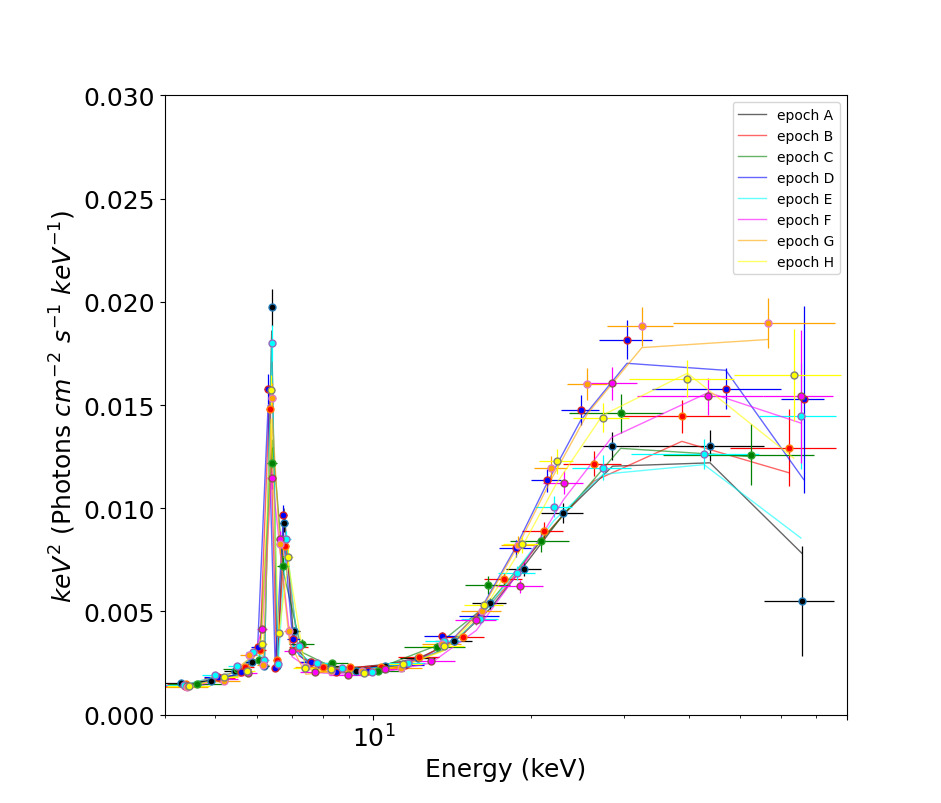
Figure 1: The eight epochs of NuSTAR FPMA spectra plotted together

AGN emit across wavelengths, and X-ray emission has been observed from all categories of AGN (Mushotzky et al., 1993). However, a large fraction of AGN are obscured in X-rays (Bianchi et al., 2012; Ramos Almeida & Ricci, 2017). The obscured AGN are further classified as Compton Thin and Compton Thick based on the density of the equivalent hydrogen column density ($\rm{N_{H}}$) along the line of sight. In a Compton Thick AGN, the central engine is surrounded by the heavily obscuring dust and gas with $\rm{N_{H}}$ $\geq$ $10^{24}$ $cm^{-2}$ embedded in a dusty torus that is located at few parsec ($\sim$ 0.1 $-$ 10 pc) from the central source (Netzer, 2015). In a Compton Thick Seyfert 2 galaxy, reflection from the torus produces a reflection hump at around 15$-$30 keV and reveals the presence of neutral Fe K$\alpha$ emission line at 6.4 keV with an equivalent width of $\sim$1 keV (Ghisellini et al. 1994; Marinucci et al. 2016). However, the nature of this obscuring material is not static. In many AGN the observed X-ray variability is likely caused due to the variation in the circumnuclear material (Risaliti et al., 2002; Yang et al., 2016).

X-ray emission from AGN is believed to originate from regions close to the central super massive black hole. Models of the X-ray emitting region include the hot corona situated close to the vicinity of the accretion disk (Haardt & Maraschi 1991, 1993) as well as the AGN relativistic jet that emanates along the black hole rotation axis (Harris & Krawczynski, 2006; Blandford et al., 2019). It is likely that the contribution of each of these physical processes to the observed X-ray emission may differ among AGN. The observed X-ray spectrum from AGN consists of many components such as (i) a power law component believed to be due to the inverse Compton scattering of the optical, ultra-violet accretion disk photons by the hot electrons in the corona (Haardt & Maraschi 1991, 1993), (ii) soft excess at energies lesser than 1 keV, which could be due to a warm ($kT_{e}$ = 1 keV) and optically thick ($\tau$ = 10 - 20) corona (Gierliński & Done, 2004; Petrucci et al., 2018) or due to relativistically blurred reflection (García et al., 2019), (iii) reflection bump beyond few keV due to scattering of X-rays by the accretion disk or distant material (Ghisellini et al., 1994) and (iv) the fluorescent Fe K$\alpha$ line with equivalent width of $\sim$1 keV(Ghisellini et al., 1994; Marinucci et al., 2016). In spite of the numerous X-ray studies on AGN, the exact causes for the origin of X-ray emission in them is still not understood. This also includes the size, shape and location of the X-ray corona in AGN. Parameters that can put constraints on the nature of the X-ray corona in AGN are the power law index ($\Gamma$) and the high energy cut-off ($E_{cut}$) in the X-ray continuum. This $E_{cut}$ in the X-ray continuum is related to the temperature of the Comptonizing electrons ($kT_{e}$) in the hot corona via E_cut = 2$-$3 $kT_{e}$ (Petrucci et al., 2001), however, there are reports for this relation to show deviation among AGN (Liu et al., 2014; Middei et al., 2019; Pal et al., 2022).

One of the constraints to get good estimate of E_cut on a large sample of AGN is the lack of high signal to noise ratio data at energies beyond 50 keV, where the cut-off in the spectrum is defined. Though more measurements are now available from instruments such as NuSTAR (Fabian et al., 2015; Buisson et al., 2018; Kamraj et al., 2018; Tortosa et al., 2018; Ricci et al., 2018; Rani & Stalin, 2018; Rani et al., 2019; Kang et al., 2020; Baloković et al., 2020; Akylas & Georgantopoulos, 2021; Hinkle & Mushotzky, 2021; Kamraj et al., 2022), it is important to increase such measurements on a larger number of sources, firstly to find good estimates of E_cut and secondly to find better constraints on the correlation of E_cut with other physical properties of the sources. Also, variation in the temperature of the corona is now known in few radio-quiet category of AGN (Zhang et al., 2018; Barua et al., 2020, 2021a; Kang et al., 2021; Wilkins et al., 2022; Pal et al., 2022), however, it is not clear if it is shown by all AGN. This is due to the lack of such studies on many AGN, mostly attributed to the paucity of homogeneous multi-epoch data on a large number of sources. Therfore it is of great importance to find more sources that are known to show variations in $kT_{e}$.

Table 1: Log of NuSTAR observations.

OBSID	Epoch	Date	Exposure Time
			(secs)
60002030002	A	2012-12-18	57850
60002030004	B	2012-12-20	48556
60002030006	C	2012-12-21	19461
60002033002	D	2014-08-18	52055
60002033004	E	2015-02-05	53685
60302003002	F	2017-07-31	49979
60302003004	G	2017-08-27	52549
60302003006	H	2017-11-06	49691

Table 2: Log of XMM-Newton observations.

OBSID	Epoch	Date	Exposure Time
			(secs)
0111200101	A	2000-07-29	42258
0111200102	B	2000-07-30	46429
0740060201	C	2014-07-10	63997
0740060301	D	2014-07-18	57600
0740060401	E	2014-08-19	54000
0740060501	F	2015-02-03	54600

NGC 1068 is one of the most studied Seyfert 2 galaxies. Situated at a redshift of $z$ = 0.0038 (Huchra et al., 1999), it is powered by a black hole of mass $M_{BH}=1.6\times 10^{7}M_{\odot}$ (Panessa et al., 2006). In X-rays the source is studied in the past (Matt et al., 2004; Bauer et al., 2015; Marinucci et al., 2016; Zaino et al., 2020). This source was first observed by Ginga in the X-ray band and the observation revealed the presence of a broad neutral Fe K$\alpha$ line (Koyama et al., 1989) with an equivalent width of $\sim$ 1.3 keV. Later on, the ASCA observations resolved the Fe lines into neutral and ionized components (Ueno et al., 1994; Iwasawa et al., 1997). It is known as an emitter of high energy $\gamma$-ray radiation in the MeV$-$GeV range (Abdollahi et al., 2020) and also has been reported as a neutrino source (Aartsen et al., 2020). In the past, the hard X-ray source spectrum was fitted with a two reflector model (Matt et al., 1997; Guainazzi et al., 1999; Bauer et al., 2015). The central engine of the source is found to be completely obscured by the dusty torus with a column density of $\rm{N_{H}}$ $\geq$ $10^{25}$ $cm^{-2}$ (Matt et al., 2000), therefore, the observer can only see the scattered emission along the line of sight. This scattered emission is commonly thought to originate from two types of reflectors, the cold reflector component that arises from Compton scattering off the primary X-ray emission from the neutral circumnuclear material, while the second warm ionized reflector component that arises due to Compton scattering off the heavily ionized material that acts as the mirror of the primary emission (Matt et al., 2004).

Using the multi epoch X-ray observations Bauer et al. (2015) fitted the spectra of NGC 1068 using the two reflector model along with different line emission, radiative recombination continuum and the off nuclear point source emission. Using XMM-Newton and NuSTAR joint fit of the NGC 1068 high energy ($>$ 4 keV) spectra Marinucci et al. (2016) detected excess flux in August 2014 observation above 20 keV by 32$\pm$6 % with respect to the previous 2012 December observation and later February 2015 observation. This transient excess above 20 keV in NGC 1068 spectra was ascribed to a drop in the absorbing column density from $\rm{N_{H}}$ $>$ 8.5 $\times$ $10^{24}$ $cm^{-2}$ to (5.9$\pm$0.4) $\times$ $10^{24}$ $cm^{-2}$ in 2012 spectra. The authors first caught the source during this unrevealing period in which the obscured material moved temporarily from the line of sight and the source was found to be its highest flux state. Recently, Zaino et al. (2020) presented the spectral analysis of the NuSTAR data taken between July 2017 and Feb 2018 to check for spectral variability. From the varying column density found in the timescale of 1 to 6 months, the authors inferred the presence of the clumpy torus structure surrounding the source. Using $\it Swift-XRT$ data the authors also detected an ultra-luminous X-ray source at a distance of $\sim$2 kpc from the nuclear region of NGC 1068.

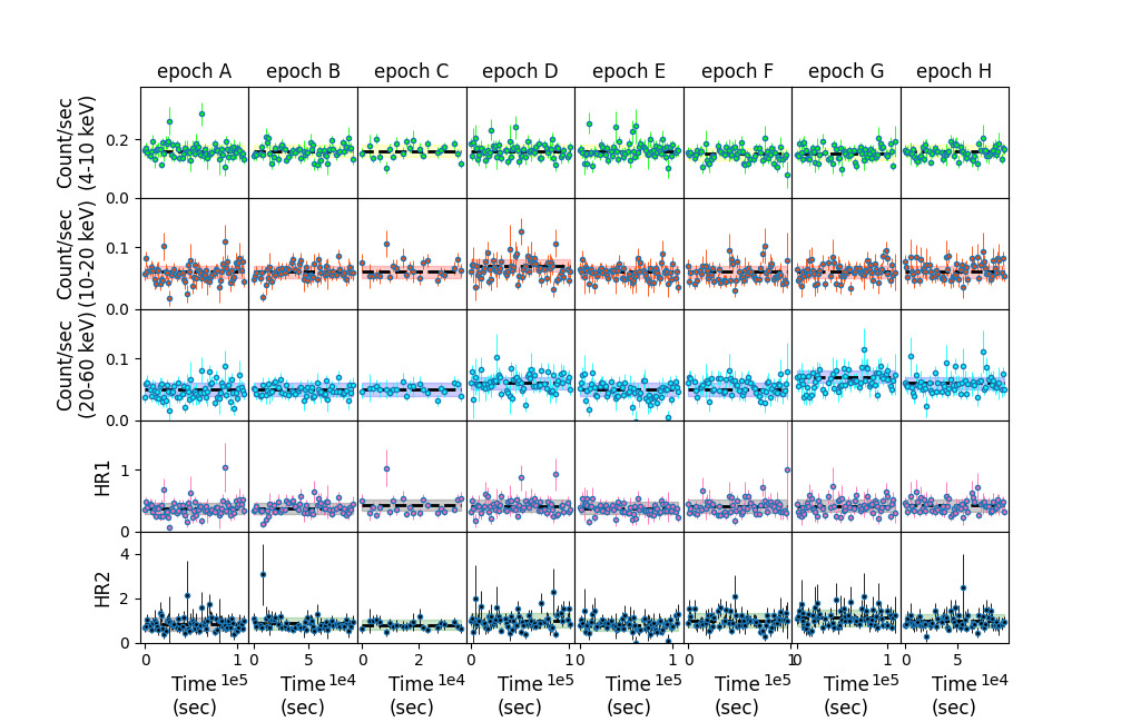
Figure 2: The NuSTAR light curves of NGC 1068 in three energy bands, 4$-$10 keV (first panel), 10$-$20 keV (second panel) and 20$-$60 keV (third panel). The HR1 and HR2 vs time are plotted in the last two panels. The black dashed lines are the mean of the count rate and HR. The shaded region in each panel is the mean errors in the count rate and HR.

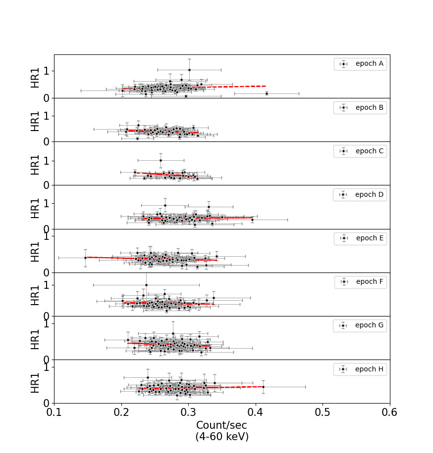
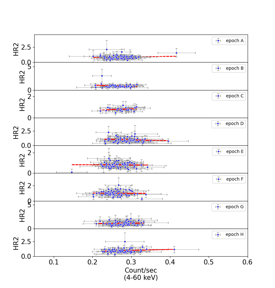
Figure 3: Left panel: The relation between HR1 and count rate in the 4$-$60 keV band. Right panel: The relation between HR2 and count rate in the 4$-$60 keV band. The red dashed lines in both panels are the linear least squares fit to the data.

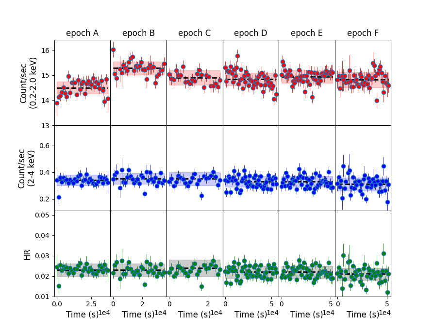
Figure 4: XMM-Newton EPIC PN light curves of NGC 1068 in two energy bands, 0.2$-$2 keV (top) and 2$-$4 keV (middle). The HR vs time is plotted in the bottom panel. The black dashed line and the shaded region in each panel is the mean value of counts/sec or HR and the corresponding errors respectively.

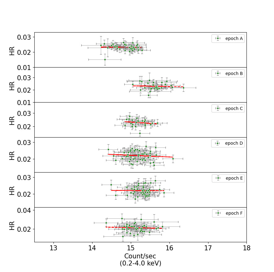
Figure 5: The relation between HR and count rate in the 0.2$-$4 keV band. The red dashed lines in both panels are the linear least square fit to the data.

Though the X-ray emission from NGC 1068 has been analysed in the past (Bauer et al. 2015, Marinucci et al. 2016, Zaino et al. 2020), the source has not been studied for variation in the temperature of the corona. Bauer et al. (2015) from a joint fit of 2$-$195 keV data from different instruments reported a $\rm{E_{cut}}$ of 128${}^{+115}_{-44}$ keV. Recently Hinkle & Mushotzky (2021) jointly fit the XMM-Newton (OBSID-0740060401) and NuSTAR (OBSID-60002033002) data and reported a $\rm{E_{cut}}$ of 28.4${}^{+7.7}_{-4.0}$ keV. In this work, taking advantage of the multiple epochs of data available from NuSTAR (along with near simultaneous XMM-Newton data at certain epochs of NuSTAR observations), we carried out for the first time an investigation of the variation in the temperature of the corona if any. In this paper, we present results of our variability analysis of NGC 1068, from observations carried out by NuSTAR between 2012 and 2017. Also, we present our results on spectral analysis of the same NuSTAR data set in conjunction with observations from XMM-Netwon. The aim was to find the temperature of the corona in this source and its variation if any. The paper is organized as follows. In Section 2, we discuss the X-ray observations with NuSTAR and XMM-Netwon and the reduction of the data, the analysis is presented in Section 3, followed by the summary of the results in the final section.

2 Observations and Data Reduction

2.1 NuSTAR

Till now, NGC 1068 was observed by NuSTAR (Harrison et al., 2013) nine times with its two co-aligned telescopes with the focal plane modules A (FPMA) and B (FPMB) respectively. In one of the epochs in the year 2018, an off-nuclear Ultra-Luminous X-ray source was detected (Zaino et al., 2020) at a distance of about $30^{\prime\prime}$ from the nuclear region of NGC 1068. Barring this epoch, we considered eight epochs of data for this work. The details of these eight epochs of observations are given in Table 1. To visualize the spectral features of these observations the best fitted model-2 FPMA spectra (see section 4) are plotted together in Fig. 1.

We reduced the NuSTAR data in the 3$-$79 keV band using the standard NuSTAR data reduction software NuSTARDAS v1.9.7 distributed by HEASARC within HEASoft v6.29. Considering the passage of the satellite through the South Atlantic Anomaly we selected SAACALC = 2, SAAMODE optimized and also excluded the tentacle region. The calibrated, cleaned, and screened event files were generated by running nupipeline task using the CALDB release 20210701. To extract the source counts we chose a circular region of radius $50^{\prime\prime}$ centered on the source. Similarly, to extract the background counts, we selected a circular region of the same radius away from the source on the same chip to avoid contamination from source photons. We then used the nuproducts task to generate energy spectra, response matrix files (RMFs) and auxiliary response files (ARFs), for both the hard X-ray detectors housed inside the corresponding focal plane modules FPMA and FPMB.

2.2 XMM-Newton

NGC 1068 was observed by XMM-Newton for eight epochs during the year 2000 to 2015. Within these we used six data sets taken between 2000 to 2015 for the timing analysis. For spectral analysis we used only three sets of data in 2014 due to their simultaneity with at least one epoch of NuSTAR observations.

We chose to use only the EPIC-PN data for the extraction of source and background spectra. The log of the OBSIDs used in this work is given in Table 2. We used SAS v1.3 for the data reduction. Only single events (PATTERN==0) with quality flag=0 were selected. The event files were filtered to exclude background flares selected from time ranges where the 10–15 keV count rates in the PN camera exceeded 0.3 c/s. Source spectra were extracted from an annular region between the inner and outer radius of $15^{\prime\prime}$ and $30^{\prime\prime}$ centered on the nucleus. Background photons were selected from a source-free region of equal area on the same chip as the source. Here we note that for the source extraction, choosing a circular region of radius $30^{\prime\prime}$ produced pile up in the first two OBSIDs. However, pile up was not noticed in the other 4 epochs. To avoid pile up and to maintain uniformity in data reduction we chose to extract the source and background from an annular region for all the six epochs. We constructed RMFs and ARFs using the tasks RMFGEN and ARFGEN for each observation.

Table 3: Mean count-rate and the mean HR in different energy bands of NGC 1068 obtained from the light curves (see Fig. 2) and the results of the correlation between HR and the total count rate (see Fig. 3).

OBSID	Epoch	Mean count rate			Mean HR		HR1		HR2
		4$-$ 10 keV	10$-$20 keV	20$-$60 keV	HR1	HR2	r	p	r	p
60002030002	A	0.16 $\pm$ 0.02	0.06 $\pm$ 0.01	0.05 $\pm$ 0.01	0.37 $\pm$ 0.09	0.85 $\pm$ 0.30	0.10	0.43	0.10	0.40
60002030004	B	0.16 $\pm$ 0.02	0.06 $\pm$ 0.01	0.05 $\pm$ 0.01	0.38 $\pm$ 0.09	0.86 $\pm$ 0.27	-0.18	0.20	-0.18	0.19
60002030006	C	0.16 $\pm$ 0.02	0.06 $\pm$ 0.01	0.05 $\pm$ 0.01	0.42 $\pm$ 0.09	0.80 $\pm$ 0.24	-0.25	0.26	0.19	0.38
60002033002	D	0.16 $\pm$ 0.02	0.07 $\pm$ 0.01	0.06 $\pm$ 0.01	0.41 $\pm$ 0.10	0.99 $\pm$ 0.32	0.04	0.78	-0.12	0.34
60002033004	E	0.16 $\pm$ 0.02	0.06 $\pm$ 0.01	0.05 $\pm$ 0.01	0.38 $\pm$ 0.10	0.80 $\pm$ 0.27	-0.16	0.21	-0.01	0.92
60302003002	F	0.15 $\pm$ 0.02	0.06 $\pm$ 0.01	0.05 $\pm$ 0.01	0.41 $\pm$ 0.11	1.00 $\pm$ 0.32	-0.07	0.58	-0.02	0.90
60302003004	G	0.15 $\pm$ 0.02	0.06 $\pm$ 0.01	0.07 $\pm$ 0.01	0.41 $\pm$ 0.10	1.12 $\pm$ 0.37	-0.16	0.22	0.07	0.57
60302003006	H	0.16 $\pm$ 0.02	0.06 $\pm$ 0.01	0.06 $\pm$ 0.01	0.42 $\pm$ 0.10	0.96 $\pm$ 0.30	0.09	0.52	0.16	0.22

3 Timing Analysis

3.1 NuSTAR

For timing analysis of the source, we utilized the data from NuSTAR and generated the background subtracted light curves with multiple corrections (e.g. bad pixel, livetime etc.) applied on the count rate in three energy bands, namely, 4$-$10 keV, 10$-$20 keV and 20$-$60 keV respectively with a bin size of 1.2 ksec. The light curves in different energy bands, along with variations in hardness ratios (HRs) are given in Fig. 2. To check for variability in the generated light curves we calculated the fractional root mean square variability amplitude ($F_{var}$;Edelson et al. 2002; Vaughan et al. 2003) for each epoch. $F_{var}$ is defined as $F_{var}=\sqrt{\frac{V^{2}-\overline{\sigma^{2}}}{\overline{x}^{2}}}$, where, $V^{2}=\frac{1}{N-1}(x_{i}-\overline{x})^{2}$ is the sample variance and $\overline{\sigma^{2}}=\frac{1}{N}\sum\sigma_{i}^{2}$ is the mean square error in the flux measurements. Here, $x_{i}$ is the observed value in counts per second, $\overline{x}$ is the arithmetic mean of the $x_{i}$ measurements, and $\sigma_{i}$ is the error in each individual measurement. The error in $F_{var}$ was estimated following Vaughan et al. (2003). For a binning choice of 1.2 ksec the calculated $F_{var}$ values indicate that the source is found not to show any significant variations within epochs. This is also evident in Fig. 2. Shown by black dashed lines in Fig. 2 is the mean brightness of the source at each epoch determined from the light curves. These mean values are given in Table 3. From light curve analysis it is evident that the source has not shown variation in the soft band (4$-$10 keV and 10$-$20 keV) during the five years of data analysed in this work. However, variation is detected in the hard band (20$-$60 keV) (Fig. 2). This is also very clear in Fig. 1.

Table 4: Results of the variability analysis in two energy bands of XMM-Newton

OBSID	Epoch	Mean count rate		Mean HR	r	p
		0.2$-$2 keV	2$-$4 keV
0111200101	A	14.50$\pm$0.24	0.34$\pm$0.04	0.023$\pm$0.003	-0.03	0.88
0111200201	B	15.28$\pm$0.26	0.35$\pm$0.04	0.023$\pm$0.003	-0.06	0.76
0740060201	C	14.86$\pm$0.25	0.34$\pm$0.04	0.023$\pm$0.003	-0.16	0.45
0740060301	D	14.85$\pm$0.25	0.33$\pm$0.04	0.022$\pm$0.003	-0.11	0.45
0740060401	E	14.94$\pm$0.25	0.33$\pm$0.04	0.022$\pm$0.003	-0.01	0.96
0740060501	F	14.82$\pm$0.30	0.31$\pm$0.05	0.021$\pm$0.003	-0.06	0.71

In the two bottom panels of Figure 2, we show the evolution of two hardness ratios, namely HR1 and HR2 during the duration of the observations analysed in this work. HR1 and HR2 are defined as: HR1 = C(10$-$20)/C(4$-$10) and HR2 = C(20$-$60)/C(10$-$20), where C(4$-$10), C(10$-$20) and C(20$-$60) are the count rates in 4$-$10 keV, 10$-$20 keV, and 20$-$60 keV respectively. For each epoch, the mean hardness ratio is shown as a black dashed line in Figure 2 and the mean values are given in Table 3. As the errors are large, no variation in the hardness ratio of the source could be ascertained between epochs. We also looked for correlation if any between the hardness ratios, HR1 and HR2 against the broad band count rate in the 4$-$60 keV band with a time binning of 1.2 ksec. This is shown in Fig. 3. Also, shown in the same figure are the linear least squares fit to the data. Calculated values of the Pearson’s rank coefficient (r) and probability for no correlation (p) from the linear least square fit are given in Table 3. Analysing those values we found no variation of hardness ratios with the brightness of the source.

3.2 XMM-Newton

Using the six epochs of XMM-Newton EPIC PN data from Table 2 we generated the light curves in two energy bands, 0.2$-$2.0 keV and 2.0$-$4.0 keV using a binning size of 1.2 ksec. The light curves along with the variation of HR are shown in Fig. 4. Here, HR is defined as the ratio of C(2.0$-$4.0) to C(0.2$-$2.0), where C(2.0$-$4.0) and C(0.2$-$2.0) are the count rates in 2.0$-$4.0 keV and 0.2$-$2.0 keV energy bands respectively. From $F_{var}$ analysis we found no significant variation within the epochs of observation. The black dashed lines in the first two panels of Fig. 4 are the mean values of the count rate in different energy bands. The mean values of the count rate (see Table 4) indicate that in the soft band (0.2$-$2 keV) the source was in its brightest state in epoch B. There is thus variation in the soft band with the source being brighter in epoch B relative to epoch A. However, in the hard band we did not find any significant change in the source brightness between epochs. In the same Table 4, the constant values of mean HR between epochs also argues for no variation in brightness state of the source. In Fig. 5 HR is plotted against the total count rate in 0.2$-$4.0 keV band. The results of the linear least squares fit are given in Table 4. From the p values we conclude that no significant correlation between HR and the total count rate is found in NGC 1068.

4 Spectral analysis

In addition to characterizing the flux variability of NGC 1068, we also aimed in this work to investigate the variation in the temperature of the corona of the source.

4.1 NuSTAR only spectral fit

To check for variation in the temperature of the corona in NGC 1068, we first concentrated on the NuSTAR data alone. For that we fitted simultaneous FPMA/FPMB data for the eight epochs of observations available in the NuSTAR archive. To avoid the host galaxy contamination we used the NuSTAR data in the 4$-$79 keV energy band (Marinucci et al., 2016). For the spectral analysis, using XSPEC version 12.12.0 (Arnaud, 1996), we fitted the background subtracted spectra from FPMA and FPMB simultaneously (without combining them) allowing the cross normalization factor to vary freely during spectral fits. The spectra were binned to have minimum 25 counts/energy bin using the task grppha. To get an estimate of the model parameters that best describe the observed data, we used the chi-square ($\chi^{2}$) statistics and for calculating the errors in the model parameters we used the $\chi^{2}$ = 2.71 criterion i.e. 90 % confidence range in XSPEC.

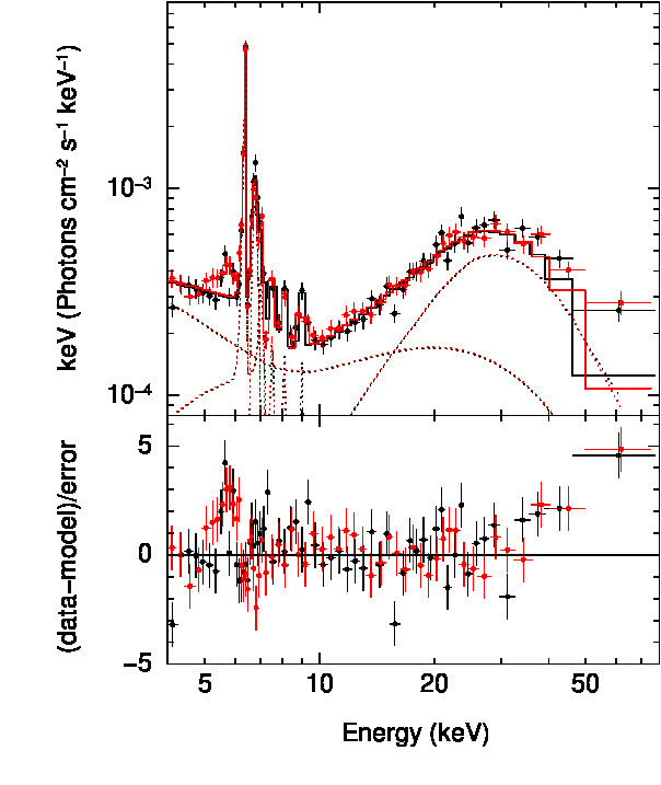
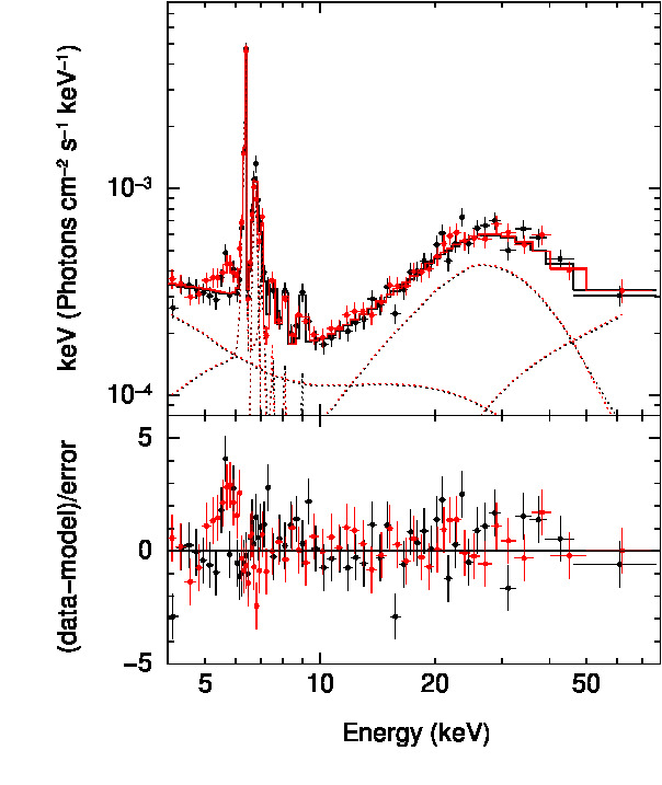
Figure 6: The best fit epoch G (with highest flux) unfolded spectra along with the data to model ratio using Model 1b (left panel) and Model 2b (right panel)

.

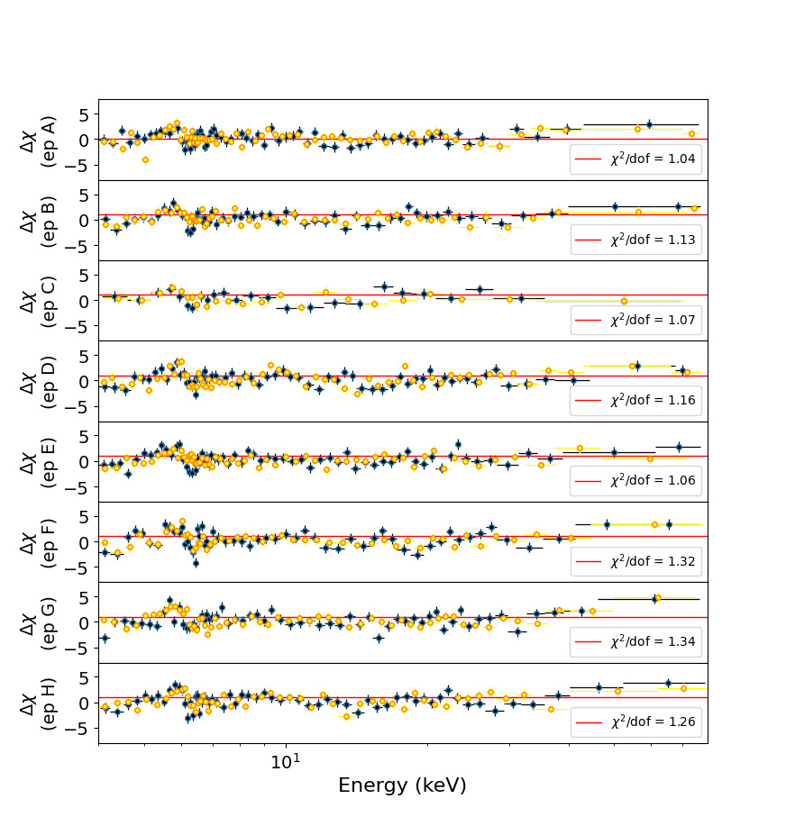
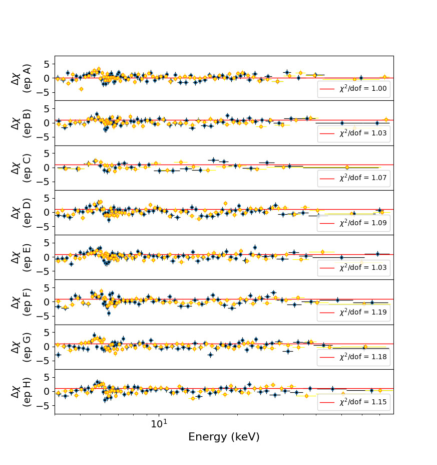
Figure 7: The data to model ratio of all eight epochs of NuSTAR observations using Model 1b (left panel) and Model 2b (right panel).

In all our model fits to the observed spectra, the const represents the cross calibration constant between the two focal plane modules FPMA and FPMB. To model the line of sight galactic absorption the phabs component was used and for this the neutral hydrogen column density ($\rm{N_{H}}$) was frozen to 3.32$\times$ $10^{20}$ atoms $cm^{-2}$ as obtained from Willingale et al. (2013). To take into account the strong emission lines seen in the observed NuSTAR spectra, we used four zgauss components in XSPEC. In all the zgauss models considered to fit the emission lines, the line energies and the normalization were kept free during the fitting while $\sigma$ was kept frozen to 0.1 keV. The redshift (z) for all the model components was kept fixed to 0.0038 (Véron-Cetty & Véron, 2010). The inclination angle which is the angle the line of sight of the observer makes with the axis of the AGN ($i$) was fixed at 63^∘ (Matt et al., 2004) in all the models.

4.1.1 Model 1

NGC 1068 has been extensively studied in the hard X-ray ($>$3 keV) band earlier (Matt et al., 1997; Matt et al., 2004; Bauer et al., 2015; Marinucci et al., 2016; Zaino et al., 2020) mostly using the two component reflector model. The main essence of this model is to fit (a) the cold and distant reflector using pexrav/pexmon/(MYTS+MYTL), and (b) the warm, ionized Compton-scattered component using power-law/cutoff power-law with Compton down scattering under the assumption that the electron temperature is much smaller than the photon energy ($m_{e}c^{2}$). Few Gaussian components were also used to model various neutral and ionized emission lines present in the source spectra. In this work too, to find the coronal temperature of the source, we modeled the source spectra using two different reflector components.

1. The self consistent Comptonization model xillverCP (García et al., 2014) that takes into account the cold and distant reflector, the neutral Fe k$\alpha$ ($\sim$ 6.4 keV) and Fe k$\beta$ ($\sim$ 7.06 keV) lines.

2. The warm ionized Compton scattered reflection using two models separately. At first, following Poutanen et al. (1996), a Compton scattered component ($f_{scat}$) for an arbitrary intrinsic continuum ($f_{intr}$). As an intrinsic continuum, we used a power-law, that was modified for Compton down scattering using equation (1) given in Poutanen et al. (1996). Secondly, the self consistent xillverCP model with a high ionization parameter ($log\xi$ = 4.7) to model the warm, ionized reflector. Here we note that fixing the ionization parameter to some other values ($log\xi$ = 3.0, 3.5 and 4.0) did not produce any significant change in the derived best fit values. It only self-consistently added few ionization lines in the model, but, the spectral shape remained unchanged. Using the Compton scattered component in place of a warm mirror may affect the spectra by adding curvature below 2 keV (Bauer et al., 2015), but the spectral modeling of the NuSTAR data above 4 keV with or without inclusion of the Compton down scattering in the warm reflector did not produce any significant effect on the derived best fit values. We also arrived at the similar conclusion from using the XMM-Newton and NuSTAR data jointly below 4 keV. This is discussed in detail in Section 4.2.

3. Gaussian components to take care of the Fe ionized ($\sim$ 6.57, 6.7 and 6.96 keV), Ni k$\alpha$ ($\sim$ 7.47 keV), Ni k$\beta$ ($\sim$ 8.23 keV) and Ni ionized ($\sim$ 7.83 keV) emission lines.

In XSPEC, the two models used in the fitting of the spectra have the following form,

$$Model1a=const*phabs*(f1*zpo+xillverCP+zgauss+zgauss+zgauss+zgauss)$$ (1)

and

$$Model1b=const*phabs*(xillverCP_{warm}+xillverCP_{cold}+zgauss+zgauss+zgauss+zgauss)$$ (2)

Here, we note that, From the data to ratio plot we did not find any prominent residuals near the line emission regions, but, in all epochs we noticed residues at around 6.0 keV (see Fig. 6 and Fig. 7). This feature at 6.0 keV has no physical origin but might appear in the NuSTAR data due to calibration issues (Zaino et al., 2020).

Model 1a: For the spectral fit with this model, we used the formula (f1) obtained from Poutanen et al. (1996) to consider the Compton down scattering of the intrinsic continuum (zpo). Following Poutanen et al. (1996),

$$f1\propto\tau_{sc}[1+\mu^{2}+xx_{1}(1-\mu)^{2}]$$ (3)

In Equation 3, $x=h\nu/m_{e}c^{2}$ is the dimensionless photon energy $\mu$ = cos i, x1 = x/[1- x(1-$\mu$)] and $\tau_{sc}$ is the Thompson optical depth of the scattering material. We considered the constant of proportionality $\times$ $\tau_{sc}$ as an another constant (p1) and kept it as a free parameter in the spectral analysis. During spectral fits the photon index ($\Gamma$) and the normalization for the two reflectors were tied together. For the cold reflector we modeled only the reflection component by fixing the reflection fraction ($R$) to $-$1 throughout. The parameters that were kept free are the relative iron abundance ($AF_{e}$), $\rm{kT_{e}}$ and p1. The constant, p1 was allowed to vary between 0.0 and 10.0 during the fit. To model the cold and neutral reflector the ionization parameter ($\xi$) was frozen to 1.0 (i.e log$\xi$ = 0). The best fit values obtained using Model 1a are given in Table 6.

Model 1b: Here, we used xillverCP twice to model the warm and cold reflection respectively. For the warm and ionized reflector we used ${\it xillverCP_{warm}}$ by fixing the ionization parameter to its highest value ($log\xi=4.7$) and for the cold and distant reflection (${\it xillverCP_{cold}}$) the reflector was considered as a neutral one with a fixed $log\xi$ of 0.0. In the modelling of the source spectra using Model 1b we tied $\Gamma$ and $\rm{kT_{e}}$ of the two reflectors together. At first, the normalization for the two reflectors were tied together and the best fit produced a $\chi^{2}$ of 637 for 484 degrees of freedom for epoch A. We then modelled the epoch A spectrum by varying the two normalization independently and got an improved $\chi^{2}$ of 504 for 483 degrees of freedom. For the other epochs we therefore carried out the model fit by leaving the two normalization untied. For both the reflectors we fixed $R$ to $-$1 to consider the reflection components only. During the fitting $AF_{e}$ between the two reflectors were tied together. The best fit unfolded spectra along with the residues of the data to Model 1b fit to the epoch G spectra are given in the left panel of Fig. 6. The best fit results of Model 1b are given in Table 6. For all the epochs the residuals of the fit are given in left panel of Fig. 7.

4.1.2 Model 2

Following Bauer et al. (2015) we then used the leaky torus model in which it is assumed that there is a finite probability for the primary emission to escape the medium without scattering or getting absorbed and partially punching through above 20 $-$ 30 keV. In a Compton-Thick AGN, the direct transmitted continuum if at all present, is not observable below $\sim$ 10 keV. In Model 2, with the two reflectors, this transmitted or the direct component was taken care of. We assumed that a direct transmitted intrinsic continuum (zpo) was attenuated by the line of sight Compton thick absorber with a column density of $\rm{N_{H}}$ = $10^{25}$ atoms $cm^{-2}$ and an inclination angle ($\theta_{incl}$) of $90^{\circ}$ (for an edge on torus). Here also, we used xillverCP with $log\xi$ = 0.0 to model the cold reflection, and, either f1*zpo (Poutanen et al., 1996) (Model 2a), or xillverCP with $log\xi$ = 4.7 (Model 2b) to take care of the warm and ionized reflection. In XSPEC the models take the following forms,

$$Model2a=const*phabs*(zpo*MYTZ+f1*zpo+xillverCP++zgauss+zgauss+zgauss+zgauss)$$ (4)

and,

$$Model2b=const*phabs*(zpo*MYTZ+xillverCP_{warm}+xillverCP_{cold}++zgauss+zgauss+zgauss+zgauss)$$ (5)

In both the models, we used the MYTZ component from the MYtorus set of models (Murphy & Yaqoob, 2009; Yaqoob, 2012) to fit the zeroth-order continuum. This is often called the direct or transmitted continuum which is simply a fraction of the intrinsic continuum that leaves the medium without being absorbed or scattered. This energy dependent zeroth-order component (MYTZ) is used as a multiplicative factor applied to the intrinsic continuum. MYTZ is purely a line-of-sight quantity and does not depend on the geometry and covering fraction of the out-of-sight material. It includes the equivalent column density ($\rm{N_{H}}$), inclination of the obscuring torus along the line of sight ($\theta_{incl}$) and the redshift of the source. During the spectral fits $\rm{N_{H}}$ and $\theta_{incl}$ were frozen to $10^{25}$ $cm^{-2}$ and $90^{\circ}$ respectively.

Model 2a: During the spectral fitting with this model $\Gamma$ and the normalization for all the transmitted and reflected components were tied together. To model the warm and cold reflectors we used f1*zpo and xillverCP respectively. The parameters for these two models were treated in a similar fashion as described in Model 1a. The best fit values obtained from Model 2a are given in Table- 6.

Model 2b: Here, $\Gamma$ of the transmitted and scattered components were tied together, but the normalization were varied independently to achieve acceptable fit statistics. For the warm and cold reflectors the model parameters were treated in a similar way as described in Model 1b. Using this model we obtained a better fit statistics than Model 1b with no prominent residues present in the hard energy part (see the right panel of Fig. 6). The best fit values are given in Table 6. For Model 2b we calculated the flux in three energy bands, i.e, 4$-$10 keV, 10$-$20 keV and 20$-$79 keV. The fluxes obtained for FPMA module ($F^{FPMA}$) are given in Table 6. In the 20 $-$ 79 keV band on epoch D (August, 2014) the source was brighter by about 22% and 28% respectively compared to the mean brightness in December 2012 (epoch A, B and C) and February 2015 (epoch E) FPMA spectra. The source brightness again increased in the 20 $-$ 79 keV band on epoch G (August 2017) and it was found to be brighter by about 32% and 36% relative to the December 2012 and February 2015 spectra respectively. For all the epochs, the best fit data to model residues are plotted in the right panel of Fig. 7.

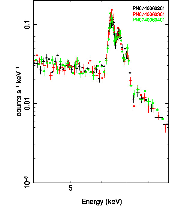
Figure 8: Three 2014 EPIC-PN spectra plotted together in the 4$-$9 keV band.

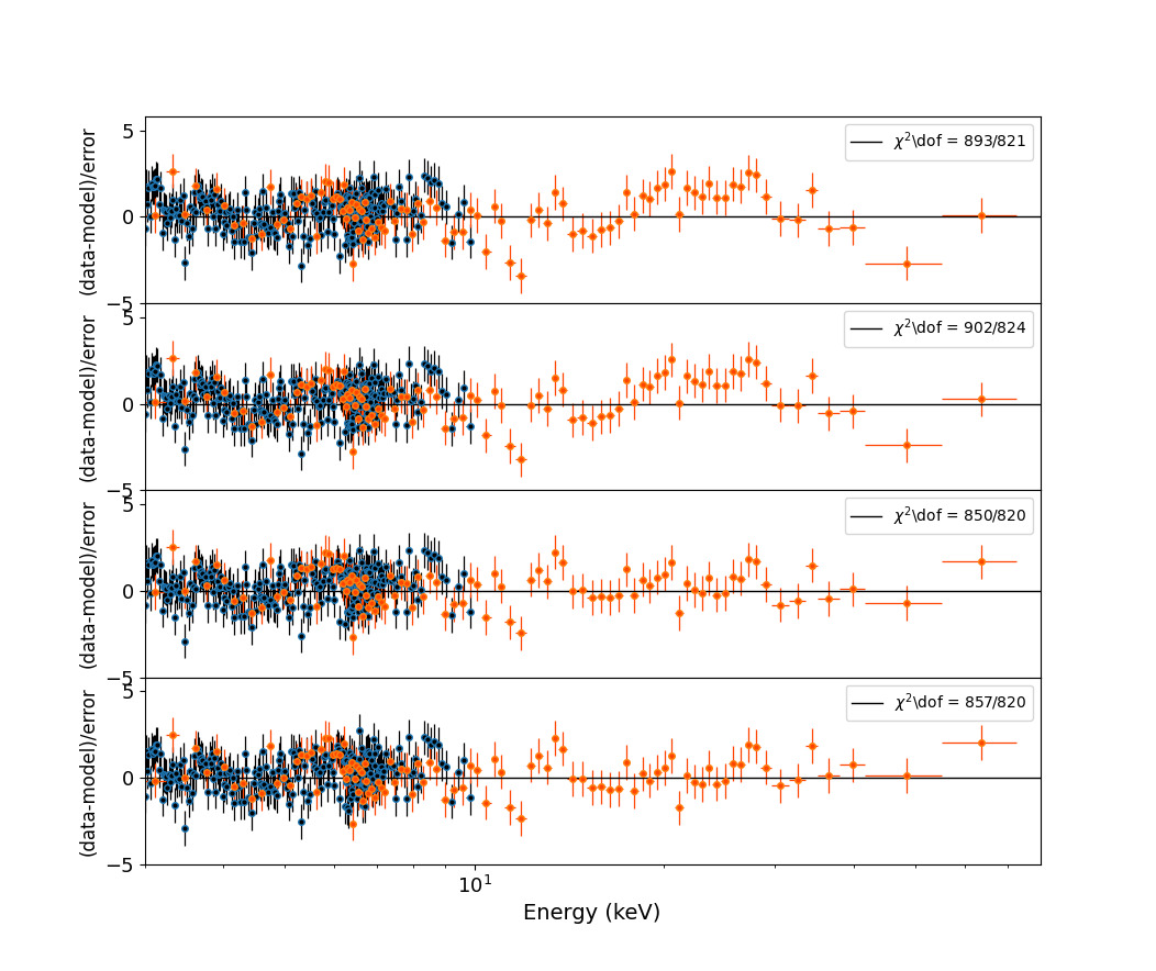
Figure 9: Best fit data to the model ratio for constant*phabs*zphabs*(cutoffpl+pexrav+zgauss(8)) (top panel) ; constant*phabs*zphabs*(f1*cutoffpl+pexrav+zgauss(8)) (2nd panel from the top) ; constant*phabs*zphabs*(MYTZ*cutoffpl+f1*cutoffpl+pexrav+zgauss(8)) (3rd panel from the top) and constant*phabs*zphabs*(zpo*MYTZ+f1*zpo+xillverCP+zgauss(6)) (bottom panel) to the XMM-Newton and NuSTAR (epoch D FPMA) spectra in the 3$-$79 keV band.

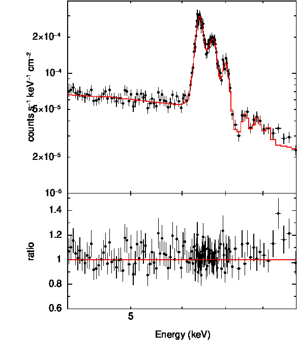
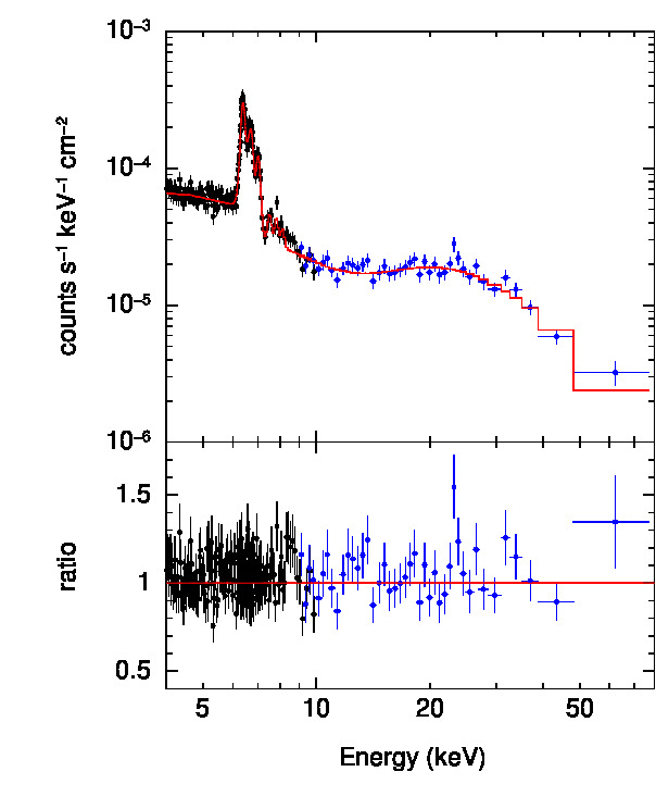
Figure 10: Left panel: Best fit EPIC-PN combined spectra in the 4$-$9 keV band. Right panel: XMM-Newton and NuSTAR (epoch D FPMA) joint best fit spectra in the 4$-$79 keV band.

Table 5: Best fit line energies along with normalization. Here, the line energy (E) is in keV and the normalization ($N_{E}$) is in units of $10^{-5}$ photons keV^-1 cm^-2 s^-1

Parameter		line		Value
E1		Fe Be-like K$\alpha$		6.60${}^{+0.03}_{-0.03}$
$N_{E1}$				1.85${}^{+0.47}_{-0.44}$
E2		Fe He-like K$\alpha$		6.75${}^{+0.02}_{-0.02}$
$N_{E2}$				2.86${}^{+0.46}_{-0.50}$
E3		Fe H–like K$\alpha$		7.02${}^{+0.01}_{-0.02}$
$N_{E3}$				1.35${}^{+0.19}_{-0.18}$
E4		Ni K$\alpha$		7.53${}^{+0.03}_{-0.03}$
$N_{E4}$				0.51${}^{+0.15}_{-0.15}$
E5		Ni ionized He-like K$\alpha$		7.86${}^{+0.04}_{-0.04}$
$N_{E5}$				0.46${}^{+0.15}_{-0.15}$
E6		Ni K$\beta$		8.15${}^{+0.08}_{-0.08}$
$N_{E6}$				0.28${}^{+0.14}_{-0.14}$

Table 6: Results of Model 1a, Model 1b, Model 2a and Model 2b fits to the simultaneous NuSTAR FPMA $-$ FPMB spectra. The $\rm{kT_{e}}$ and the line energies (E1, E2, E3 and E4) are in units of keV. Column densities ($N_{H}$) are in unit of $cm^{-2}$. Flux (F) is expressed in unit of $10^{-11}$ erg $cm^{-2}$ $s^{-1}$. Normalization of components (N) in different models at 1 keV are in units of photons $keV^{-1}$ $cm^{-2}$ $s^{-1}$. Parameters with the star (*) mark represent the frozen values.

Model	Parameter	epoch A	epoch B	epoch C	epoch D	epoch E	epoch F	epoch G	epoch H
1a	$\Gamma$	1.33${}^{+0.03}_{-0.03}$	1.30${}^{+0.03}_{-0.03}$	1.32${}^{+0.05}_{-0.06}$	$<$1.21	1.32${}^{+0.03}_{-0.03}$	$<$1.22	$<$1.21	$<$1.22
	$\rm{A_{Fe}}$	4.79${}^{+0.71}_{-0.37}$	5.00*	4.87${}^{+1.50}_{-0.57}$	4.38${}^{+0.30}_{-0.32}$	4.34${}^{+0.36}_{-0.36}$	4.93${}^{+0.47}_{-0.35}$	4.46${}^{+0.30}_{-0.30}$	4.40${}^{+0.30}_{-0.30}$
	$\rm{kT_{e}}$	7.60${}^{+0.47}_{-0.41}$	7.48${}^{+0.35}_{-0.32}$	8.04${}^{+0.78}_{-0.69}$	7.44${}^{+0.28}_{-0.27}$	6.82${}^{+0.36}_{-0.32}$	7.26${}^{+0.25}_{-0.29}$	7.60${}^{+0.29}_{-0.28}$	7.29${}^{+0.29}_{-0.28}$
	N $\times(10^{-4})$	1.31${}^{+0.10}_{-0.10}$	1.35${}^{+0.07}_{-0.08}$	1.33${}^{+0.17}_{-0.15}$	1.60${}^{+0.08}_{-0.08}$	1.50${}^{+0.11}_{-0.10}$	1.43${}^{+0.08}_{-0.08}$	1.61${}^{+0.09}_{-0.09}$	1.53${}^{+0.09}_{-0.09}$
	p1	1.28${}^{+0.24}_{-0.20}$	1.23${}^{+0.16}_{-0.14}$	1.31${}^{+0.35}_{-0.31}$	0.70${}^{+0.11}_{-0.10}$	0.93${}^{+0.18}_{-0.16}$	0.76${}^{+0.10}_{-0.11}$	0.66${}^{+0.11}_{-0.10}$	0.69${}^{+0.11}_{-0.10}$
	$\chi^{2}/dof$	468/482	437/421	210/199	483/468	436/452	473/414	528/449	479/429
	E1	6.75${}^{+0.03}_{-0.03}$	6.79${}^{+0.03}_{-0.03}$	6.79${}^{+0.05}_{-0.05}$	6.77${}^{+0.03}_{-0.03}$	6.78${}^{+0.03}_{-0.03}$	6.77${}^{+0.03}_{-0.03}$	6.80${}^{+0.03}_{-0.03}$	6.79${}^{+0.03}_{-0.03}$
	$N_{E1}$ $\times(10^{-5})$	3.82${}^{+0.42}_{-0.47}$	3.50${}^{+0.45}_{-0.42}$	3.61${}^{+0.37}_{-0.69}$	3.39${}^{+0.46}_{-0.43}$	3.40${}^{+0.45}_{-0.42}$	2.64${}^{+0.44}_{-0.41}$	2.88${}^{+0.42}_{-0.40}$	3.39${}^{+0.44}_{-0.43}$
	E2	7.59${}^{+0.09}_{-0.09}$	7.58${}^{+0.16}_{-0.13}$	7.62${}^{+0.16}_{-0.15}$	7.45${}^{+0.18}_{-0.16}$	7.51${}^{+0.14}_{-0.18}$	7.61${}^{+0.10}_{-0.09}$	7.66${}^{+0.15}_{-0.13}$	7.55${}^{+0.09}_{-0.10}$
	$N_{E2}$ $\times(10^{-5})$	0.81${}^{+0.21}_{-0.22}$	0.55${}^{+0.21}_{-0.21}$	0.80${}^{+0.41}_{-0.44}$	0.46${}^{+0.23}_{-0.24}$	0.55${}^{+0.25}_{-0.28}$	0.62${}^{+0.21}_{-0.21}$	0.56${}^{+0.21}_{-0.20}$	0.62${}^{+0.23}_{-0.23}$
	E3	8.19${}^{+0.12}_{-0.16}$	8.46${}^{+0.17}_{-0.17}$	8.07${}^{+0.16}_{-0.15}$	7.96${}^{+0.11}_{-0.11}$	7.95${}^{+0.20}_{-0.17}$	8.33${}^{+0.13}_{-0.14}$	8.03${}^{+0.23}_{-0.21}$	8.08${}^{+0.08}_{-0.09}$
	$N_{E3}$ $\times(10^{-5})$	0.45${}^{+0.19}_{-0.19}$	0.48${}^{+0.19}_{-0.19}$	0.74${}^{+0.41}_{-0.41}$	0.65${}^{+0.22}_{-0.23}$	0.43${}^{+0.26}_{-0.25}$	0.38${}^{+0.19}_{-0.18}$	0.55${}^{+0.23}_{-0.27}$	0.56${}^{+0.21}_{-0.21}$
	E4	8.77${}^{+0.11}_{-0.12}$	8.75${}^{+0.10}_{-0.11}$	-	8.63${}^{+0.18}_{-0.23}$	8.87${}^{+0.17}_{-0.36}$	9.12${}^{+0.19}_{-0.18}$	9.00${}^{+0.14}_{-0.14}$	9.00${}^{+0.26}_{-0.29}$
	$N_{E4}$ $\times(10^{-6})$	3.69${}^{+1.74}_{-1.79}$	3.28${}^{+1.20}_{-1.25}$	-	2.79${}^{+1.79}_{-1.79}$	3.84${}^{+1.72}_{-1.72}$	2.15${}^{+1.69}_{-1.63}$	4.19${}^{+1.80}_{-1.79}$	2.75${}^{+1.76}_{-1.76}$
	$\rm{C_{FPMA/FPMB}}$	1.04${}^{+0.03}_{-0.03}$	1.03${}^{+0.03}_{-0.03}$	1.01${}^{+0.05}_{-0.04}$	1.01${}^{+0.03}_{-0.03}$	1.02${}^{+0.03}_{-0.03}$	1.00${}^{+0.03}_{-0.03}$	1.01${}^{+0.03}_{-0.03}$	0.98${}^{+0.03}_{-0.03}$
1b	$\Gamma$	1.34${}^{+0.05}_{-0.03}$	1.26${}^{+0.08}_{-0.06}$	$<$1.27	$<$1.24	1.31${}^{+0.04}_{-0.05}$	$<$1.26	$<$1.22	$<$1.26
	$\rm{A_{Fe}}$	$<$7.05	$<$6.31	$>$7.29	5.08${}^{+1.31}_{-0.23}$	5.83${}^{+1.86}_{-1.00}$	6.82${}^{+0.95}_{-1.78}$	5.50${}^{+0.69}_{-0.59}$	5.53${}^{+1.52}_{-0.68}$
	$\rm{kT_{e}}$	9.10${}^{+0.13}_{-0.16}$	8.95${}^{+0.16}_{-0.20}$	9.38${}^{+0.18}_{-0.18}$	8.75${}^{+0.16}_{-0.12}$	8.69${}^{+0.22}_{-0.25}$	8.68${}^{+0.17}_{-0.23}$	8.77${}^{+0.13}_{-0.14}$	8.78${}^{+0.16}_{-0.16}$
	$N_{\it xillverCP_{warm}}$ $\times(10^{-5})$	2.43${}^{+0.24}_{-0.34}$	2.29${}^{+0.36}_{-0.36}$	2.68${}^{+0.15}_{-0.49}$	2.03${}^{+0.30}_{-0.16}$	1.90${}^{+0.35}_{-0.26}$	1.95${}^{+0.18}_{-0.35}$	1.99${}^{+0.15}_{-0.19}$	2.02${}^{+0.31}_{-0.23}$
	$N_{\it xillverCP_{cold}}$ $\times(10^{-4})$	1.03${}^{+0.08}_{-0.06}$	1.12${}^{+0.09}_{-0.10}$	1.00${}^{+0.11}_{-0.08}$	1.38${}^{+0.07}_{-0.09}$	1.18${}^{+0.10}_{-0.10}$	1.22${}^{+0.10}_{-0.08}$	1.39${}^{+0.07}_{-0.07}$	1.27${}^{+0.10}_{-0.09}$
	$\chi^{2}/dof$	504/483	474/420	213/199	545/468	480/452	545/414	600/449	545/431
2a	$\Gamma$	1.32${}^{+0.03}_{-0.03}$	1.30${}^{+0.04}_{-0.04}$	1.32${}^{+0.05}_{-0.05}$	$<$1.22	1.32${}^{+0.03}_{-0.03}$	$<$1.22	$<$1.21	$<$1.22
	$\rm{A_{Fe}}$	4.78${}^{+0.70}_{-0.37}$	5.50${}^{+1.14}_{-0.77}$	4.77${}^{+1.47}_{-0.60}$	4.43${}^{+0.31}_{-0.32}$	4.32${}^{+0.38}_{-0.37}$	5.00${}^{+0.63}_{-0.37}$	4.56${}^{+0.31}_{-0.32}$	4.33${}^{+0.37}_{-0.34}$
	$\rm{kT_{e}}$	7.39${}^{+0.41}_{-0.69}$	7.80${}^{+0.49}_{-0.58}$	7.28${}^{+0.86}_{-0.62}$	7.45${}^{+0.30}_{-0.29}$	6.35${}^{+0.46}_{-0.34}$	7.51${}^{+0.33}_{-0.37}$	7.43${}^{+0.35}_{-0.55}$	6.80${}^{+0.51}_{-0.35}$
	p1	0.79${}^{+0.69}_{-0.21}$	1.34${}^{+0.20}_{-0.18}$	0.83${}^{+0.53}_{-0.35}$	0.74${}^{+0.11}_{-0.10}$	0.53${}^{+0.25}_{-0.19}$	0.88${}^{+0.11}_{-0.11}$	0.64${}^{+0.12}_{-0.31}$	0.72${}^{+0.10}_{-0.11}$
	$\chi^{2}/dof$	467/482	421/420	205/199	480/468	431/452	449/414	521/449	476/431
2b	$\Gamma$	1.35${}^{+0.09}_{-0.07}$	1.50${}^{+0.08}_{-0.08}$	1.49${}^{+0.13}_{-0.13}$	1.31${}^{+0.06}_{-0.04}$	1.37${}^{+0.03}_{-0.03}$	1.35${}^{+0.04}_{-0.03}$	1.32${}^{+0.06}_{-0.05}$	1.34${}^{+0.05}_{-0.05}$
	$\rm{A_{Fe}}$	6.09${}^{+2.43}_{-1.44}$	4.39${}^{+0.76}_{-0.70}$	4.48${}^{+1.63}_{-0.95}$	4.98${}^{+0.56}_{-0.63}$	5.00*	5.00${}^{+0.71}_{-0.41}$	4.43${}^{+0.72}_{-0.68}$	4.31${}^{+0.67}_{-0.66}$
	$\rm{kT_{e}}$	8.97${}^{+0.22}_{-0.30}$	8.51${}^{+0.49}_{-0.82}$	9.13${}^{+0.63}_{-0.98}$	8.76${}^{+0.15}_{-0.39}$	8.55${}^{+0.17}_{-0.16}$	8.57${}^{+0.17}_{-0.32}$	8.46${}^{+0.39}_{-0.66}$	8.30${}^{+0.45}_{-0.72}$
	$\chi^{2}/dof$	481/481	433/419	211/198	507/467	464/452	495/415	529/448	496/430
	$F_{4-10}^{FPMA}$	0.42	0.42	0.43	0.41	0.42	0.38	0.39	0.40
	$F_{10-20}^{FPMA}$	0.45	0.45	0.48	0.49	0.45	0.42	0.48	0.47
	$F_{20-79}^{FPMA}$	2.23	2.50	2.55	3.09	2.24	2.92	3.54	2.97

4.2 XMM-Newton & NuSTAR Joint fit

Fitting the NuSTAR spectra alone could not handle the line emission profiles present in the source spectrum properly. To model the lines we used three XMM-Newton EPIC PN spectra taken in 2014 along with the NuSTAR FPMA data. Use of XMM-Newton data jointly with NuSTAR, the observations of which are not simultaneous requires the source to be non-variable. We show in Fig. 8 all three XMM-Newton PN spectra taken in 2014. This figure indicates that the source has not shown any noticeable variation in line and continuum flux. Also, in all the eight epochs of NuSTAR data accumulated over a period of 5 years, no variation in the soft band (4$-$10 keV) is observed (see Table 3 and Fig. 2). Therefore, it is not inappropriate to jointly model the NuSTAR and XMM-Newton observations. We combined the three XMM-Newton EPIC PN spectra together using the task epicspeccombine and then binned the spectra with 25 counts/bin using the task specgroup.

We carried out joint model fits to the 3-10 keV XMM-Newton 2014 combined spectra with the 3-79 keV epoch D NuSTAR spectrum. To account for both warm and cold reflection, several models were tried. Firstly, we used a cutoffpl to model the warm reflector that did not take into account Compton down scattering. For modelling the cold reflector we used pexrav (Magdziarz & Zdziarski, 1995) with R=-1. We obtained the best fit values of 1.59${}^{+0.09}_{-0.09}$, 95${}^{+100}_{-47}$ and 11.22${}^{+3.51}_{-2.70}$ for $\Gamma$, $\rm{E_{cut}}$ and $\rm{A_{Fe}}$ respectively with a $\chi^{2}$ of 893 for 821 degrees of freedom. Using this model we got an acceptable fit statistics with a mild hump between 20 $-$ 30 keV energy range (see top panel of Fig. 9). We replaced the cutoffpl with xillver with a fixed $\log\xi$ = 4.7 to account for the Compton down scattering. We obtained $\Gamma$ = 1.54${}^{+0.04}_{-0.04}$, $\rm{E_{cut}}$ = 94${}^{+26}_{-19}$ and $\rm{A_{Fe}}$ $>$ 9.15. This fit produced a $\chi^{2}$ of 884 for 821 degrees of freedom. We then replaced xillver with f1*cutoffpl (for f1, see Equation 3) to model the warm reflector and obtained $\Gamma$ = 1.62${}^{+0.11}_{-0.11}$, $\rm{E_{cut}}$ = 97${}^{+149}_{-39}$ and $\rm{A_{Fe}}$ = 11.50${}^{+4.54}_{-3.11}$ with a $\chi^{2}$ of 902 for 824 degrees of freedom. With or without the inclusion of Compton down scattering in the warm reflector we obtained similar set of best fit values and a hump in the data to model residue plot near 25 keV (see first two panels of Fig. 9). We thus conclude that inclusion of Compton down scattering in the warm reflection has insignificant effect on the derived parameters.

The spectrum of the Compton-Thick AGN is refection dominated, however, there is a finite probability for the primary emission to be transmitted (above $>$10 keV) through the Compton thick absorber. Thus, we modified our model to take into account the transmitted primary emission by including the (MYTZ*cutoffpl) component into the previously described two reflector models in which the cold reflection was modelled using pexrav with R=-1. For the warm reflector we first used xillver with R=-1 and $log\xi$ = 3.1. For the Compton absorber along the line of sight we assumed a column density of $10^{25}$ $cm^{-2}$ with an inclination of $90^{\circ}$ (Bauer et al., 2015). We obtained $\Gamma$ $<$1.28, $\rm{E_{cut}}$ = 16${}^{+2}_{-1}$ and $\rm{A_{Fe}}$ = $>$7.41 with a $\chi^{2}$ of 847 for 820 degrees of freedom. The fit statistics now improved by $\Delta\chi^{2}$ = 37 over the reduction of 1 degree of freedom and the hump around 20 $-$ 30 keV band was also taken care of. We obtained a similar fit with $\Gamma$ = 1.37${}^{+0.18}_{-0.16}$, $\rm{E_{cut}}$ = 18${}^{+4}_{-3}$ and $\rm{A_{Fe}}$ = 5.68${}^{+4.20}_{-2.41}$ with a $\chi^{2}$ of 850 for 820 degrees of freedom from using f1*cutoffpl (see Equation 3) as a warm reflector. Inclusion of the transmitted primary emission with the two reflector model described the source spectra well with a harder photon index and lower $\rm{E_{cut}}$ with no prominent features present in the data to model ratio plot at high energies (see 3rd panel of Fig. 9). Previously also, NGC 1068 X-ray spectrum was modelled with a flatter photon index. From a joint analysis of XMM-Newton epoch E spectrum with the epoch D NuSTAR spectrum Hinkle & Mushotzky (2021) reported $\Gamma$ = 1.21${}^{+0.13}_{-0.07}$. From modelling the 0.5$-$10 keV ASCA observation Ueno et al. (1994) found a best fit $\Gamma$ of 1.28$\pm$0.14. Replacing pexrav with xillverCP to model the cold reflector with R=-1 and $log\xi$ = 0.0 we obtained $\Gamma$ = 1.26${}^{+0.03}_{-0.03}$, $\rm{kT_{e}}$ = 8.59${}^{+0.40}_{-0.37}$ and $\rm{A_{Fe}}$ = 4.02${}^{+0.36}_{-0.33}$ with a $\chi^{2}$ = 857 for 820 degrees of freedom. The data to the best fit model residues are given in Fig. 9.

To estimate $\rm{kT_{e}}$ we used Model 2b, as described earlier for the NuSTAR spectral fit alone. Here the NuSTAR FPMA spectra for all the epochs in the 9 $-$ 79 keV along with the combined 2014 XMM-Newton data in the 4 $-$ 10 keV band were used to take care of the line emission region carefully. We used six Gaussian components to model all the ionized and neutral lines present in the spectra. The line energies and the normalization were kept free during the fitting while the line widths were frozen to 0.01 keV. The self-consistent $xillverCP_{cold}$ model took care of the neutral Fe k$\alpha$ ($\sim$ 6.4 keV) and k$\beta$ ($\sim$ 7.08 keV) lines, wherein the first three Gaussian components were used to model the ionized Fe lines at energies $\sim$ 6.57 keV (Fe Be-like K$\alpha$), 6.67 keV (Fe He-like K$\alpha$) and 6.96 keV (Fe H–like K$\alpha$). The neutral Ni k$\alpha$ ($\sim$ 7.47 keV), Ni k$\beta$ ($\sim$ 8.23 keV) and Ni ionized He-like K$\alpha$ ($\sim$ 7.83 keV) were taken care by the other three Gaussian components. As seen from the left panel of Fig. 10 we did not find any prominent residue in the 4$-$9 keV band. All the best fitted line energies and the normalization are given in Table 5. The best fit model parameters along with their corresponding errors are given in Table 7. We found that this joint fit produced similar best fit values as obtained from NuSTAR fit alone. The best fit model to the data (the combined EPIC PN data and NuSTAR FPMA epoch D spectra) along with the residue is shown in the right panel of Fig 10.

Table 7: Results of the analysis of the Model 2b fit to the XMM-Newton and NuSTAR FPMA spectra in the 4 $-$ 79 keV energy band. $\rm{kT_{e}}$ is in unit of keV and column densities ($N_{H}$) are in units of $cm^{-2}$. Normalization of components (N) at 1 keV is in unit of photons $keV^{-1}cm^{-2}s^{-1}$.

Parameter	epoch A	epoch B	epoch C	epoch D	epoch E	epoch F	epoch G	epoch H
$N_{H}^{ztbabs}$	9.78${}^{+2.92}_{-2.96}$	9.19${}^{+2.73}_{-2.75}$	7.09${}^{+5.04}_{-4.19}$	9.57${}^{+2.39}_{-2.60}$	9.16${}^{+2.58}_{-2.72}$	9.72${}^{+2.37}_{-2.55}$	9.51${}^{+2.75}_{-3.15}$	8.90${}^{+2.64}_{-2.88}$
$\Gamma$	1.29${}^{+0.07}_{-0.08}$	1.33${}^{+0.15}_{-0.07}$	1.48${}^{+0.11}_{-0.25}$	$<$1.32	1.33${}^{+0.10}_{-0.06}$	1.28${}^{+0.07}_{-0.05}$	1.26${}^{+0.07}_{-0.10}$	1.30${}^{+0.07}_{-0.07}$
$\rm{A_{Fe}}$	6.08${}^{+3.87}_{-1.59}$	4.89${}^{+2.89}_{-1.51}$	3.09${}^{+4.96}_{-1.08}$	4.19${}^{+1.44}_{-0.93}$	4.75${}^{+2.19}_{-0.63}$	4.99${}^{+1.70}_{-1.10}$	3.90${}^{+1.33}_{-1.10}$	3.81${}^{+1.27}_{-1.01}$
$\rm{kT_{e}}$	8.69${}^{+0.28}_{-0.33}$	8.62${}^{+0.33}_{-0.49}$	8.07${}^{+0.59}_{-0.75}$	8.59${}^{+0.30}_{-0.36}$	8.60${}^{+0.34}_{-0.58}$	8.68${}^{+0.26}_{-0.38}$	8.55${}^{+0.25}_{-0.41}$	8.48${}^{+0.35}_{-0.51}$
$\chi^{2}/dof$	592/584	576/565	516/492	620/586	590/574	613/569	630/584	585/578
$\rm{C_{XMM/NuSTAR}}$	0.96${}^{+0.08}_{-0.08}$	0.95${}^{+0.08}_{-0.07}$	0.94${}^{+0.11}_{-0.11}$	0.94${}^{+0.08}_{-0.08}$	0.93${}^{+0.08}_{-0.08}$	0.98${}^{+0.08}_{-0.08}$	0.93${}^{+0.08}_{-0.08}$	0.97${}^{+0.08}_{-0.09}$

5 Summary

In this work, we carried out spectral and timing analysis of eight epochs of NuSTAR observations performed between December 2012 and November 2017 probing time scales within epochs and between epochs that spans about 5 years. The timing analysis of the six XMM-Newton observations between July 2000 and February 2015 was also performed. We also carried out the spectral analysis of the 2014 combined XMM-Newton EPIC PN and NuSTAR FPMA data jointly. The results of this work are summarized below

1. We found the source not to show flux variation within each of the eight epochs of NuSTAR observation.

2. Between epochs, that span the time-scales from 2012 to 2017, we found variation in the source. Here too, the source did not show variation in the soft energy range. As in agreement with the earlier results by Marinucci et al. (2016) and Zaino et al. (2020), we also found that the observed variations is only due to variation in the energy range beyond 20 keV. This too was noticed in Epoch D (August 2014) and Epoch G (August 2017), when the brightness of the source beyond 20 keV was higher by about 20% and 30% respectively relative to the three NuSTAR observations in the year 2012.

3. From timing analysis, we observed no correlation of spectral variation (hardness ratio) with brightness.

4. Fitting physical models to the observed data we could determine the temperature of the corona in NGC 1068 with values ranging from 8.46${}^{+0.39}_{-0.66}$ keV and 9.13${}^{+0.63}_{-0.98}$ keV. However, we found no variation in the temperature of the corona during the 8 epochs of observations that span a duration of about 5 years.

5. From the timing analysis of six XMM-Newton EPIC PN data we found no significant flux variation both in between and within epochs of observation in the hard band. In the soft band too we found the source did not show any significant flux variation within epochs but it was brighter in epoch B compared to epoch A.

6. The combined spectral fit of XMM-Newton and NuSTAR data provided results that are in agreement with those obtained by model fits to the NuSTAR data alone.

In NGC 1068, we did not find evidence for variation in the temperature of the corona from analysis of data that span more than five years. This is evident from the best fit values of $\rm{kT_{e}}$ from Table 6. Also, the results from various models are found to be similar. The values of $\rm{kT_{e}}$ found for NGC 1068 also lie in the range of $\rm{kT_{e}}$ found in other AGN. Measurements of $\rm{E_{cut}}$ are available for a large number of AGN that includes both Seyfert 1 and Seyfert 2 type. However, studies on the variation of $\rm{E_{cut}}$ or $\rm{kT_{e}}$ are limited to less than a dozen AGN (Ballantyne et al., 2014; Ursini et al., 2015, 2016; Keek & Ballantyne, 2016; Zoghbi et al., 2017; Zhang et al., 2018; Barua et al., 2020; Kang et al., 2021; Barua et al., 2021b; Pal et al., 2022). Even in sources where $\rm{E_{cut}}$/$\rm{kT_{e}}$ variations are known, the correlation of the variation of $\rm{kT_{e}}$ with various physical properties of the sources are found to be varied among sources (Barua et al., 2020, 2021b; Kang et al., 2021; Pal et al., 2022). These limited observations do indicate that we do not yet understand the complex corona of AGN including its geometry and composition. Investigation of this kind needs to be extended for many AGN to better constrain the nature of corona.

Data Availability

All data used in this work are publicly available in the NuSTAR (https://heasarc.gsfc.nasa.gov/docs/nustar/nustar_archive.html) and XMM-Newton (http://nxsa.esac.esa.int) science archive.

References

- Aartsen et al. (2020) Aartsen M. G., et al., 2020, Phys. Rev. Lett., 124, 051103
- Abdollahi et al. (2020) Abdollahi S., et al., 2020, ApJS, 247, 33
- Akylas & Georgantopoulos (2021) Akylas A., Georgantopoulos I., 2021, A&A, 655, A60
- Antonucci (1993) Antonucci R., 1993, ARA&A, 31, 473
- Antonucci & Miller (1985) Antonucci R. R. J., Miller J. S., 1985, ApJ, 297, 621
- Arnaud (1996) Arnaud K. A., 1996, XSPEC: The First Ten Years. p. 17
- Awaki et al. (1991) Awaki H., Koyama K., Inoue H., Halpern J. P., 1991, PASJ, 43, 195
- Ballantyne et al. (2014) Ballantyne D. R., et al., 2014, ApJ, 794, 62
- Baloković et al. (2020) Baloković M., et al., 2020, ApJ, 905, 41
- Barua et al. (2020) Barua S., Jithesh V., Misra R., Dewangan G. C., Sarma R., Pathak A., 2020, MNRAS, 492, 3041
- Barua et al. (2021a) Barua S., Jithesh V., Misra R., Dewangan G. C., Sarma R., Pathak A., Medhi B. J., 2021a, ApJ, 921, 46
- Barua et al. (2021b) Barua S., Jithesh V., Misra R., Dewangan G. C., Sarma R., Pathak A., Medhi B. J., 2021b, The Astrophysical Journal, 921, 46
- Bauer et al. (2015) Bauer F. E., et al., 2015, The Astrophysical Journal, 812, 116
- Bianchi et al. (2012) Bianchi S., Maiolino R., Risaliti G., 2012, Advances in Astronomy, 2012, 782030
- Blandford et al. (2019) Blandford R., Meier D., Readhead A., 2019, ARA&A, 57, 467
- Buisson et al. (2018) Buisson D. J. K., Fabian A. C., Lohfink A. M., 2018, MNRAS, 481, 4419
- Edelson et al. (2002) Edelson R., Turner T. J., Pounds K., Vaughan S., Markowitz A., Marshall H., Dobbie P., Warwick R., 2002, ApJ, 568, 610
- Fabian et al. (2015) Fabian A. C., Lohfink A., Kara E., Parker M. L., Vasudevan R., Reynolds C. S., 2015, MNRAS, 451, 4375
- García et al. (2014) García J., et al., 2014, ApJ, 782, 76
- García et al. (2019) García J. A., et al., 2019, ApJ, 871, 88
- Ghisellini et al. (1994) Ghisellini G., Haardt F., Matt G., 1994, MNRAS, 267, 743
- Gierliński & Done (2004) Gierliński M., Done C., 2004, MNRAS, 349, L7
- Guainazzi et al. (1999) Guainazzi M., et al., 1999, MNRAS, 310, 10
- Haardt & Maraschi (1991) Haardt F., Maraschi L., 1991, ApJ, 380, L51
- Haardt & Maraschi (1993) Haardt F., Maraschi L., 1993, ApJ, 413, 507
- Harris & Krawczynski (2006) Harris D. E., Krawczynski H., 2006, ARA&A, 44, 463
- Harrison et al. (2013) Harrison F. A., et al., 2013, ApJ, 770, 103
- Hinkle & Mushotzky (2021) Hinkle J. T., Mushotzky R., 2021, MNRAS, 506, 4960
- Huchra et al. (1999) Huchra J. P., Vogeley M. S., Geller M. J., 1999, ApJS, 121, 287
- Iwasawa et al. (1997) Iwasawa K., Fabian A. C., Matt G., 1997, MNRAS, 289, 443
- Kamraj et al. (2018) Kamraj N., Harrison F. A., Baloković M., Lohfink A., Brightman M., 2018, ApJ, 866, 124
- Kamraj et al. (2022) Kamraj N., et al., 2022, arXiv e-prints, p. arXiv:2202.00895
- Kang et al. (2020) Kang J., Wang J., Kang W., 2020, ApJ, 901, 111
- Kang et al. (2021) Kang J.-L., Wang J.-X., Kang W.-Y., 2021, MNRAS, 502, 80
- Keek & Ballantyne (2016) Keek L., Ballantyne D. R., 2016, MNRAS, 456, 2722
- Koyama et al. (1989) Koyama K., Inoue H., Tanaka Y., Awaki H., Takano S., Ohashi T., Matsuoka M., 1989, PASJ, 41, 731
- Liu et al. (2014) Liu T., Wang J.-X., Yang H., Zhu F.-F., Zhou Y.-Y., 2014, ApJ, 783, 106
- Magdziarz & Zdziarski (1995) Magdziarz P., Zdziarski A. A., 1995, Monthly Notices of the Royal Astronomical Society, 273, 837
- Marinucci et al. (2016) Marinucci A., et al., 2016, MNRAS, 456, L94
- Matt et al. (1997) Matt G., et al., 1997, A&A, 325, L13
- Matt et al. (2000) Matt G., Fabian A. C., Guainazzi M., Iwasawa K., Bassani L., Malaguti G., 2000, MNRAS, 318, 173
- Matt et al. (2004) Matt G., Bianchi S., Guainazzi M., Molendi S., 2004, A&A, 414, 155
- Middei et al. (2019) Middei R., Bianchi S., Marinucci A., Matt G., Petrucci P. O., Tamborra F., Tortosa A., 2019, A&A, 630, A131
- Murphy & Yaqoob (2009) Murphy K. D., Yaqoob T., 2009, MNRAS, 397, 1549
- Mushotzky et al. (1993) Mushotzky R. F., Done C., Pounds K. A., 1993, ARA&A, 31, 717
- Netzer (2015) Netzer H., 2015, ARA&A, 53, 365
- Pal et al. (2022) Pal I., Stalin C. S., Mallick L., Rani P., 2022, A&A, 662, A78
- Panessa et al. (2006) Panessa F., Bassani L., Cappi M., Dadina M., Barcons X., Carrera F. J., Ho L. C., Iwasawa K., 2006, A&A, 455, 173
- Petrucci et al. (2001) Petrucci P. O., et al., 2001, ApJ, 556, 716
- Petrucci et al. (2018) Petrucci P. O., Ursini F., De Rosa A., Bianchi S., Cappi M., Matt G., Dadina M., Malzac J., 2018, A&A, 611, A59
- Poutanen et al. (1996) Poutanen J., Sikora M., Begelman M. C., Magdziarz P., 1996, The Astrophysical Journal, 465, L107
- Ramos Almeida & Ricci (2017) Ramos Almeida C., Ricci C., 2017, Nature Astronomy, 1, 679
- Rani & Stalin (2018) Rani P., Stalin C. S., 2018, ApJ, 856, 120
- Rani et al. (2019) Rani P., Stalin C. S., Goswami K. D., 2019, MNRAS, 484, 5113
- Ricci et al. (2018) Ricci C., et al., 2018, MNRAS, 480, 1819
- Risaliti et al. (2002) Risaliti G., Elvis M., Nicastro F., 2002, ApJ, 571, 234
- Tortosa et al. (2018) Tortosa A., Bianchi S., Marinucci A., Matt G., Petrucci P. O., 2018, A&A, 614, A37
- Ueno et al. (1994) Ueno S., Mushotzky R. F., Koyama K., Iwasawa K., Awaki H., Hayashi I., 1994, PASJ, 46, L71
- Urry & Padovani (1995) Urry C. M., Padovani P., 1995, PASP, 107, 803
- Ursini et al. (2015) Ursini F., et al., 2015, A&A, 577, A38
- Ursini et al. (2016) Ursini F., et al., 2016, MNRAS, 463, 382
- Vaughan et al. (2003) Vaughan S., Edelson R., Warwick R. S., Uttley P., 2003, MNRAS, 345, 1271
- Véron-Cetty & Véron (2010) Véron-Cetty M. P., Véron P., 2010, A&A, 518, A10
- Wilkins et al. (2022) Wilkins D. R., Gallo L. C., Costantini E., Brandt W. N., Blandford R. D., 2022, MNRAS,
- Willingale et al. (2013) Willingale R., Starling R. L. C., Beardmore A. P., Tanvir N. R., O’Brien P. T., 2013, MNRAS, 431, 394
- Yang et al. (2016) Yang G., et al., 2016, ApJ, 831, 145
- Yaqoob (2012) Yaqoob T., 2012, MNRAS, 423, 3360
- Zaino et al. (2020) Zaino A., et al., 2020, MNRAS, 492, 3872
- Zhang et al. (2018) Zhang J.-X., Wang J.-X., Zhu F.-F., 2018, ApJ, 863, 71
- Zoghbi et al. (2017) Zoghbi A., et al., 2017, ApJ, 836, 2