Pion-mediated Cooper pairing of neutrons: beyond the bare vertex approximation

Abstract

In some quantum many particle systems, the fermions could form Cooper pairs by exchanging intermediate bosons. This then drives a superconducting phase transition or a superfluid transition. Such transitions should be theoretically investigated by using proper non-perturbative methods. Here we take the neutron superfluid transition as an example and study the Cooper pairing of neutrons mediated by neutral $\pi$-mesons in the low density region of a neutron matter. We perform a non-perturbative analysis of the neutron-meson coupling and compute the pairing gap $\Delta$, the critical density $\rho_{c}$, and the critical temperature $T_{c}$ by solving the Dyson-Schwinger equation of the neutron propagator. We first carry out calculations under the widely used bare vertex approximation and then incorporate the contribution of the lowest-order vertex correction. This vertex correction is not negligible even at low densities and its importance is further enhanced as the density increases. The transition critical line on density-temperature plane obtained under the bare vertex approximation is substantially changed after including the vertex correction. These results indicate that the vertex corrections play a significant role and need to be seriously taken into account.

I Introduction

A large part of physical laws, ranging from the fundamental forces between elementary particles to the emergent phenomena in quantum many-body systems, can be described by certain types of fermion-boson interactions Itzykson . In the standard model, quarks and leptons are coupled to a number of intermediate gauge bosons. In nuclear matter, protons and neutrons interact with each other by exchanging mesons Walecka . In metals, the mutual influence between itinerant electrons and lattice vibrations is well captured by an effective electron-phonon coupling AGD . If a fermion-boson coupling is sufficiently weak, one can employ the perturbation expansion method to compute various physical quantities Itzykson ; AGD . However, the perturbation theory becomes invalid or at least very inaccurate in fermion-boson interacting models that do not contain any small parameter. It is also inapplicable when a system undergoes a phase transition. For instance, in some interacting fermionic systems the fermion-boson coupling leads to Cooper pairing of fermions, which then drives a phase transition towards a superconducting phase BCS or a superfluid phase Migdal60 , depending on whether fermions carry charges or not. A physically analogous phase transition occurs in QCD: the strong quark-gluon interaction generates large dynamical masses for the originally light quarks via the formation of quark-antiquark pairs Roberts00 . These phase transitions are essentially non-perturbative and cannot be investigated by means of the perturbation expansion method. It is of paramount importance to develop suitable non-perturbative methods to deal with interacting fermion-boson systems in which the perturbation theory breaks down.

For fermion-boson systems, the interaction-induced effects on the single particle properties are embodied in the fully renormalized fermion and boson propagators, which are classified as two-point correlation functions in quantum field theory Itzykson . The fermion and boson propagators satisfy two self-consistently coupled Dyson-Schwinger (DS) integral equations Itzykson ; Roberts00 . While these two DS equations are exact and absolutely non-perturbative, they are not self-closed and thus extremely hard to solve. In these two equations there is an unknown fermion-boson vertex function. This vertex function is defined in terms of a three-point correlation function and also satisfies its own DS equation, which is related to more complicated correlation functions. In fact, there exist an infinite hierarchy of DS equations that connect all the $n$-point correlation functions Itzykson ; Roberts00 . It is certainly not possible to solve the complete set of DS equations.

The DS equations could be made self-closed if some truncation schemes are introduced by hands. A widely used truncation is to simply ignore all the vertex corrections, which amounts to replacing the full vertex function with the bare vertex. Under such an approximation, the DS equations of fermion and boson propagators become self-closed and can be solved to investigate the interaction effects. The bare vertex approximation has been extensively applied to study dynamical fermion (e.g., quark) mass generation in gauge field theories Roberts00 and to investigate phonon-mediated superconductivity in various condensed matter systems Migdal ; Eliashberg ; Scalapino . For the theorists working on relativistic QED and QCD, the bare vertex approximation is known as the rainbow approximation Roberts00 . In condensed-matter community, the self-closed DS equation of the fermion propagator obtained under the bare vertex approximation is called Migdal-Eliashberg (ME) equation Migdal ; Eliashberg ; Scalapino . An obvious fact is that this truncation scheme is justified only when the vertex corrections are sufficiently small. In 1958, Migdal Migdal made a careful analysis of the lowest order (one-loop level) vertex correction to the electron-phonon coupling and argued that its magnitude is proportional to the factor $\lambda\omega_{D}/E_{F}$, where $\lambda$ is a dimensional coupling constant, $\omega_{D}$ is phonons’ Debye frequency, and $E_{F}$ is Fermi energy. This factor is at the order of $0.01\sim 0.1$ in ordinary metals, thus it is safe to ignore vertex corrections to the electron-phonon coupling. Over the last sixty years, the ME equations have been playing a major role in the theoretical studies of phonon-mediated superconductivity. It is interesting to notice that the ME-level DS equations have also been applied to investigate the properties of phonon-induced nucleon superfluid pairing in finite nuclei Terasaki02 and to treat the neutron pairing due to the coupling of the neutrons to the collective excitations of crustal lattice based on a Coulomb lattice model of neutron star crusts Sedrakian98 . Nevertheless, there exist a larger number of fermion-boson interacting systems in which the vertex corrections are not small Fernandes ; Liu21 . To describe these systems, it is necessary to go beyond the bare vertex approximation and incorporate vertex corrections into the DS equations properly.

In this paper, we take the neutron superfluid transition as an example and study whether the ME equations provide a reliable description of this transition. The concept of neutron-pairing induced superfluid was first conceived by Migdal Migdal60 in 1960, motivated by the microscopic theory of superconductivity developed by Bardeen, Cooper, and Schrieffer (BCS) in 1957 BCS . In nuclear physics it is well established Walecka that nucleons (protons and neutrons) experience an attractive force at large distances and a repulsive force at small distances. For a many particle system composed of neutrons, the long-range attraction binds two neutrons together to form a Cooper pair, similar to the Cooper pairing of two electrons caused by the phonon-mediated attraction in superconductors BCS . At low temperatures, the neutron matter enters into a superfluid phase once long-range phase coherence develops among the Cooper pairs of neutrons. Interestingly, it has been suggested Margueron ; Mao ; Sun10 ; Sun ; Stein that superfluid phase would undergo a crossover between Bose-Einstein condensate (BEC) state and BCS state as the density becomes sufficiently low. We will not discuss such a crossover in this paper and focus on the pure superfluid phase. Currently, a widely accepted notion Glendenningbook ; Shapiro ; Pagereview is that neutron superfluid exists in the crust and out-core regions of neutron stars and has an important influence on both the dynamic and thermal evolutions of neutron stars. Therefore, neutron superfluid transition deserves a serious theoretical investigation.

Previous theoretical studies on neutron superfluid transition are dominantly based on the BCS mean-field theory (see review papers Lombardoreview ; Sedrakian19 ; Baldo10 and references therein), using an effective neutron-neutron pairing interaction as the starting point. Such a pairing interaction is characterized by a phenomenological potential $V(r)$, which is regarded realistic if it fits the experimental data of scattering phase-shift with a high precision. A generic agreement Lombardoreview ; Sedrakian19 is that neutrons undergo a ${}^{1}S_{0}$-wave pairing at low densities $\rho$ and a ${}^{3}PF_{2}$-wave pairing at higher densities. Although previous BCS-level studies have made considerable progress, this method has its own limitations. First, the mean-field treatment neglects many potentially important effects, such as the retardation of neutron-neutron interaction and the frequency dependence of various quantities, and is valid only when the coherence length is large enough, which is not the case for neutron systems. As pointed out in Ref. Lombardoreview , BCS mean-field results appear to be unreliable even in the ultra-low density limit. Second, the BCS pairing model contains a set of unknown free parameters, which cannot be fixed when high-precision experimental data are not available. Indeed, the realistic potential used in BCS-level calculations could be determined by phase shifts only below the energy scale of roughly $350$MeV Lombardoreview ; Baldo98 ; Elgaroy98 . Thus BCS mean-field theory is out of control in neutron matters (such as neutron star) in which the scattering energies are too high to be explored by laboratory experiments.

Here we would take a different route to study neutron superfluid transition. We prefer not to deal with a phenomenological neutron-neutron potential. Alternatively, we assume that the Cooper pairing of neutrons results from the Yukawa-type neutron-meson interactions. In neutron matters there might exist several sorts of mesons. In order to generate both the long-range attraction and short-range repulsion, one normally needs to couple neutrons to four kinds of mesons Walecka ; Glendenningbook ; Walecka74 ; Hirose07 ; Kucharek91 including pseudoscalar $\pi$-meson, scalar $\sigma$-meson, pseudovector $\rho$-meson, and vector $\omega$-meson. The roles played by these mesons rely on the values of neutron density, and these mesons cooperate to yield a realistic neutron-neutron potential. The total Lagrangian would contain four different neutron-meson interactions, possibly with additional self-interactions of mesons Boguta77 and inter-meson interactions Muller96 . Although such a model is extremely complicated and nearly intractable, we believe it important to investigate this model seriously. On the one hand, the effects ignored by BCS mean-field theory can be naturally taken into account within this model. On the other hand, this model provides a framework to study the superfluid transition and the equation of states of neutron stars in a unified manner, while BCS mean-field theory is applicable solely to superfluid transition.

Given that the complicated neutron-meson interacting model is difficult to handle, we have to break down the daunting task into a series of simpler steps. We would first find a proper method to treat a simplified model that contains only one single neutron-meson interaction and then include other kinds of mesons one by one. In this paper, we take the first step and consider only one type of meson. We suppose the neutron density $\rho$ is smaller than $0.1\rho_{0}$, where the saturation density is $\rho_{0}\simeq 0.17\mathrm{fm}^{-3}$, corresponding to relatively large mean neutron distance $r$. In this region, $\pi$-mesons (i.e., pions) play a dominant role. Since neutrons do not carry electric charge, they are only coupled to neutral pion, denoted by $\pi^{0}$. Other mesons, such as $\sigma$ and $\omega$, must be included at higher densities ($\rho>0.1\rho_{0}$) to generate the short-range repulsion, but are relatively unimportant in the low-density region. We should further assume that $\rho$ is not too small in order to avoid the possible BCS-BEC crossover. Although the model describing the Yukawa-type interaction between neutrons and $\pi^{0}$, hereafter dubbed $\pi N$ interaction, seems to have a simple form, it is a strongly interacting model because its effective coupling constant $f_{\pi}$ is at the order of unity. Therefore, the perturbative expansion method is invalid. We will employ the non-perturbative DS equation approach to investigate the superfluid transition driven by the $\pi N$ interaction. Different from mean-field calculations, the retardation effects of $\pi N$ interaction are naturally included in the DS equations at the outset. Moreover, since the meson propagator is dynamical, the frequency-momentum dependence of various quantities can be directly obtained from the DS equation results.

We will first perform a DS equation study of the $\pi N$ model based on the widely used ME (i.e., bare vertex) approximation. We derive and solve the self-consistent integral equations of the pairing function $\Delta_{s}(p)$ and the renormalization function of neutron energy $A_{0}(p)$ at a series of values of temperature and neutron density. After solving the coupled equations of $\Delta_{s}(p)$ and $A_{0}(p)$ numerically, we obtain the energy-momentum dependence of the ${}^{1}S_{0}$-wave pairing gap $\Delta(p)=\Delta_{s}(p)/A_{0}(p)$, extract the critical temperature $T_{c}$ and the critical density $\rho_{c}$ of the superfluid transition, and plot a global phase diagram on the $T$-$\rho$ plane.

Then we examine the impact of vertex corrections on the results calculated under the bare vertex approximation. At present, it is hard to compute all the vertex corrections. As the first step, we consider the one-loop vertex correction and compute its value in the zero-energy and zero-momentum limits. Our finding is that the one-loop vertex correction is not negligible even at very low neutron densities and that its importance is further enhanced as the density increases. Once the contribution of one-loop vertex correction is incorporated, the ME results of $\rho_{c}$ and $T_{c}$ are substantially changed. It appears that the ME theory breaks down and ignoring vertex corrections leads to unreliable results about the superfluid transition.

The rest of the paper is organized as follows. We define the effective model of the $\pi N$ interaction in Sec. II and derive the DS integral equations satisfied by the neutron propagator, the pion propagator, and the $\pi N$ interaction vertex function in Sec. III. In Sec. IV, we introduce the bare vertex approximation and decompose the DS equation of neutron propagator into two self-consistent integral equations of the neutron pairing function and the renormalization function of the neutron energy. We then solve the integral equations to obtain the energy-momentum dependence of these two functions. Based on the numerical results, we obtain the transition critical line and show the phase diagram. Next, in Sec. V we analyze the relative importance of the one-loop vertex correction and make a comparison between the critical lines determined with and without vertex corrections. We summarize the main results and discuss how to improve the theoretical analysis of this work in Sec. VI. We provide some calculational details in Appendix A.

II Model

Although neutron stars were predicted to exist in the universe by Landau Shapiro and independently by Zwicky and Baade Baade34 early in 1930s, they had been clearly identified Gold68 only three decades later after the group led by Hewish Hewish68 observed pulsars. Neutron stars provide a unique platform to study a variety of intriguing phenomena that are traditionally investigated separately in astrophysics, particle physics, nuclear physics, and condensed matter physics. In particular, it is interesting to explore the neutron superfluid phase Migdal60 by analyzing the observational data of neutron stars. Neutron superfluid is believed to have a significant impact on both the dynamic and thermal evolutions of neutron stars (for a recent extensive review, see Ref. Pagereview ). The pulsar glitches, which refers to the abrupt change of spin period, are very likely due to the relative motion of neutron superfluid to normal fluid Baym69 . In addition, some neutron stars, such as Cassiopeia A Ho09 , are found to cool down at a unusually high speed. The underlying mechanism of fast cooling remains unclear, although a long list of scenarios have been proposed Pagereview . Most of these scenarios rely on the existence of neutron superfluid Pagereview .

To understand the dynamic and thermal evolutions of neutron stars, it is necessary to determine the conditions for neutron superfluid to occur and compute some important quantities with high precision, such as the pairing gap $\Delta(\varepsilon,\mathbf{p})$ at neutron energies $\varepsilon$ and neutron momenta $\mathbf{p}$, the critical temperature $T_{c}$, and the critical neutron density $\rho_{c}$. Motivated by this ultimate goal, but apparently without the ambition of solving the problem immediately, here we study the pion-mediated Cooper pairing of neutron by using the DS equation approach. As explained in Sec. I, in this paper we focus on the low neutron density region and consider only neutral $\pi^{0}$-mesons. The impact of other mesons will be taken into account in the future.

The Lagrangian density describing the $\pi N$ interaction is of the form

$$\mathcal{L} = \mathcal{L}_{n}+\mathcal{L}_{\pi^{0}}+\mathcal{L}_{{\pi^{0}}nn}$$ (1)

$$= \overline{\Psi}_{n}(x)\left(i\gamma^{\mu}\partial_{\mu}-M_{N}\right)\Psi_{n}(x)+\frac{1}{2}\left(\partial_{\mu}\phi_{0}\partial^{\mu}\phi_{0}-m_{\pi}\phi_{0}^{2}\right)-ig_{\pi NN}\overline{\Psi}_{n}(x)\gamma^{5}\Psi_{n}(x)\phi_{0}(x).$$

Here, $x=(t,\mathbf{x})$ denotes the $(1+3)$-dimensional coordinate vector in real space. $M_{N}$ is the neutron mass, $m_{\pi}$ is the $\pi^{0}$ mass, and $g_{\pi NN}$ is the coupling constant of relativistic $\pi N$ Lagrangian density. $\phi_{0}$ is a one-component real scalar field, representing the $\pi^{0}$-meson. The spinor field $\Psi_{n}$, whose conjugate is $\overline{\Psi}_{n}=\Psi_{n}^{{\dagger}}\gamma^{0}$, has four components. There are five $4\times 4$ Dirac matrices, defined as follows

$$\gamma^{0}=\begin{bmatrix}\sigma_{0}&0\\ 0&-\sigma_{0}\end{bmatrix},\gamma^{1}=\begin{bmatrix}0&\sigma_{1}\\ -\sigma_{1}&0\end{bmatrix},\gamma^{2}=\begin{bmatrix}0&\sigma_{2}\\ -\sigma_{2}&0\end{bmatrix},\gamma^{3}=\begin{bmatrix}0&\sigma_{3}\\ -\sigma_{3}&0\end{bmatrix},$$

$$\gamma^{5}=i\gamma^{0}\gamma^{1}\gamma^{2}\gamma^{3}=\begin{bmatrix}0&\sigma_{0}\\ \sigma_{0}&0\end{bmatrix},$$ (2)

where $\sigma_{1}$, $\sigma_{2}$, and $\sigma_{3}$ are standard Pauli matrices of spin space and $\sigma_{0}$ is the unit $2\times 2$ matrix. The spinor field $\Psi_{n}$ satisfies the Dirac equation and can be expanded as

$$\Psi_{n}(x)=\sum_{s=\uparrow,\downarrow}\int\frac{d^{3}\mathbf{p}}{(2\pi)^{3}}\left[\alpha_{s}(\mathbf{p},t)\mu_{s}(\mathbf{p})e^{i\mathbf{p}\cdot\mathbf{x}}+\beta^{\ast}_{s}(\mathbf{p},t)\nu_{s}(\mathbf{p})e^{-i\mathbf{p}\cdot\mathbf{x}}\right].$$ (3)

Here, $\alpha_{s}(\mathbf{p},t)=\alpha_{s}(\mathbf{p})e^{-i\varepsilon t}$, $\beta_{s}(\mathbf{p},t)=\beta_{s}(\mathbf{p})e^{-i\varepsilon t}$, $\mu_{s}(\mathbf{p})=N\left[\varphi_{s},\frac{(\bm{\sigma}\cdot\mathbf{p})}{\varepsilon+M_{N}}\varphi_{s}\right]^{T}$ and $\nu_{s}(\mathbf{p})=N\left[\frac{(\bm{\sigma}\cdot\mathbf{p})}{\varepsilon+M_{N}}\varphi_{-s},\varphi_{-s}\right]^{T}$, where $\varepsilon=+\sqrt{\mathbf{p}^{2}+M_{N}^{2}}$ and $N=\sqrt{\frac{\varepsilon+M_{N}}{2M_{N}}}$, represent the positive and negative frequency solutions of $\Psi_{n}$, respectively. $\varphi_{s}$ is the basis of two-component spin space with subscripts $s=\uparrow,\downarrow$ standing for two spin directions. Defining $\alpha_{s}(\mathbf{p},t)=\sqrt{\frac{M_{N}}{\varepsilon}}a_{s}(\mathbf{p})e^{-i\varepsilon t}$ and $\beta_{s}(\mathbf{p},t)=\sqrt{\frac{M_{N}}{\varepsilon}}b_{s}(\mathbf{p})e^{-i\varepsilon t}$ for the requirement of second quantization, we re-write $\Psi_{n}(x)$ as

$$\Psi_{n}(x)=\sum_{s=\uparrow,\downarrow}\int\frac{d^{3}\mathbf{p}}{(2\pi)^{3}}\sqrt{\frac{M_{N}}{\varepsilon}}\left[a_{s}(\mathbf{p})\mu_{s}(\mathbf{p})e^{-ipx}+b^{\ast}_{s}(\mathbf{p})\nu_{s}(\mathbf{p})e^{ipx}\right],$$ (4)

where $p=(\varepsilon,\mathbf{p})$ denotes the $(1+3)$-dimensional momentum vector.

To study the Cooper pairing of neutrons, it is convenient to define a Nambu spinor Nambu60 in terms of the neutron field $\Psi_{n}(x)$. Such a Nambu spinor would have eight components since $\Psi_{n}$ already has four components. This formal complexity can be reduced if we consider the non-relativistic limit of the model. Since the neutron density is supposed to be sufficiently low, the Fermi momentum is quite small, which allows us to take the non-relativistic limit. A detailed discussion of the non-relativistic limit of the originally relativistic $\pi N$ model is presented in Ref. Weise . In this limit, the anti-neutron contributions can be omitted and the neutron momentum becomes relatively unimportant compared to its static mass $(\varepsilon\approx M_{N})$. The field $\Psi_{n}$ and its conjugate are defined as

$$\Psi_{n}(x) = \sum_{s=\uparrow,\downarrow}\int\frac{d^{3}\mathbf{p}}{(2\pi)^{3}}a_{s}(\mathbf{p})\mu_{s}(\mathbf{p})e^{-ipx},$$ (5)

$$\overline{\Psi}_{n}(x) = \sum_{s^{\prime}=\uparrow,\downarrow}\int\frac{d^{3}\mathbf{p^{\prime}}}{(2\pi)^{3}}a^{\ast}_{s^{\prime}}(\mathbf{p^{\prime}})\overline{\mu}_{s^{\prime}}(\mathbf{p^{\prime}})e^{ip^{\prime}x},$$ (6)

where $\mu_{s}(\mathbf{p})=\left[\varphi_{s},\frac{(\bm{\sigma}\cdot\mathbf{p})}{2M_{N}}\varphi_{s}\right]^{T}$ and $\overline{u}_{s^{\prime}}(\mathbf{p})=\left[\varphi^{\dagger}_{s^{\prime}},-\frac{(\bm{\sigma}\cdot\mathbf{p^{\prime}})}{2M_{N}}\varphi^{{\dagger}}_{s^{\prime}}\right]$. Substituting Eq. (5) and Eq. (6) back to the $\mathcal{L}_{\pi^{0}nn}$ term of Lagrangian density (1), we obtain

$$\mathcal{L}_{\pi^{0}nn} = -ig_{\pi NN}\sum_{s^{\prime},s=\uparrow,\downarrow}\int\frac{d^{3}\mathbf{p^{\prime}}d^{3}\mathbf{p}}{(2\pi)^{6}}\left[a^{\ast}_{s^{\prime}}(\mathbf{p^{\prime}})\overline{\mu}_{s^{\prime}}(\mathbf{p^{\prime}})e^{ip^{\prime}x}\right]\gamma^{5}\left[a_{s}(\mathbf{p})\mu_{s}(\mathbf{p})e^{-ipx}\right]\phi_{0}(q)$$ (7)

$$= -ig_{\pi NN}\sum_{s^{\prime},s=\uparrow,\downarrow}\int\frac{d^{3}\mathbf{p^{\prime}}d^{3}\mathbf{p}}{(2\pi)^{6}}a^{\ast}_{s^{\prime}}(\mathbf{p^{\prime}})a_{s}(\mathbf{p})\begin{bmatrix}\varphi^{\dagger}_{s^{\prime}}&-\frac{(\bm{\sigma}\cdot\mathbf{p^{\prime}})}{2M_{N}}\varphi^{\dagger}_{s^{\prime}}\end{bmatrix}\begin{bmatrix}0&\sigma_{0}\\ \sigma_{0}&0\end{bmatrix}\begin{bmatrix}\varphi_{s}\\ \frac{(\bm{\sigma}\cdot\mathbf{p})}{2M_{N}}\varphi_{s}\end{bmatrix}e^{i(p^{\prime}-p)x}\phi_{0}(q)$$

$$= ig_{\pi NN}\sum_{s^{\prime},s=\uparrow,\downarrow}\int\frac{d^{3}\mathbf{p^{\prime}}d^{3}\mathbf{p}}{(2\pi)^{6}}a^{\ast}_{s^{\prime}}(\mathbf{p^{\prime}})a_{s}(\mathbf{p})\left[\frac{1}{2M_{N}}\varphi^{{\dagger}}_{s^{\prime}}\bm{\sigma}\cdot(\mathbf{p^{\prime}}-\mathbf{p})\varphi_{s}\right]e^{i(p^{\prime}-p)x}\phi_{0}(q).$$

Then we re-define the neutron field operator in the non-relativistic limit as

$$\psi_{n}(x) = \sum_{s=\uparrow,\downarrow}\int\frac{d^{3}\mathbf{p}}{(2\pi)^{3}}a_{s}(\mathbf{p})\varphi_{s}e^{-ipx},$$ (8)

$$\psi^{{\dagger}}_{n}(x) = \sum_{s^{\prime}=\uparrow,\downarrow}\int\frac{d^{3}\mathbf{p^{\prime}}}{(2\pi)^{3}}a^{\ast}_{s^{\prime}}(\mathbf{p^{\prime}})\varphi^{{\dagger}}_{s^{\prime}}e^{ip^{\prime}x}.$$ (9)

Using Eq. (8) and Eq. (9), the Yukawa-coupling term is converted into

$$\mathcal{L}_{\pi^{0}nn}=-\frac{g_{\pi NN}}{2M_{N}}\bm{\nabla}\cdot\left[\psi_{n}^{{\dagger}}(x)\bm{\sigma}\psi_{n}(x)\right]\phi_{0}(x),$$ (10)

which is equivalent to

$$\mathcal{L}_{\pi^{0}nn}=\frac{f_{\pi}}{m_{\pi}}\left[\psi_{n}^{{\dagger}}(x)\bm{\sigma}\psi_{n}(x)\right]\cdot\bm{\nabla}\phi_{0}(x).$$ (11)

Here, the coupling constants appearing in Eq. (10) and Eq. (11) are related to each other by the relation $\frac{f_{\pi}}{m_{\pi}}=\frac{g_{\pi NN}}{2M_{N}}$ in non-relativistic limit Weise . The value of the coupling constant $f_{\pi}$ has already been fixed by experiments Weise : $\frac{f^{2}_{\pi}}{4\pi}\approx 0.08$, or equivalently $f_{\pi}\approx 1.0$. The neutron mass is $M_{N}\approx 940\mathrm{MeV}$ and the pion mass is $m_{\pi}\approx 135\mathrm{MeV}$. After performing Fourier transformations, we now obtain the total Lagrangian density in the following non-relativistic form

$$\mathcal{L} = \mathcal{L}_{n}+\mathcal{L}_{\pi^{0}}+\mathcal{L}_{{\pi^{0}}nn}$$ (12)

$$= \psi_{n}^{{\dagger}}(p)\left(\varepsilon-\xi_{\mathbf{p}}\right)\psi_{n}(p)+\frac{1}{2}\phi_{0}^{{\dagger}}(q)\left(\omega^{2}-\mathbf{q}^{2}-m^{2}_{\pi}\right)\phi_{0}(q)+i\frac{f_{\pi}}{m_{\pi}}\psi_{n}^{{\dagger}}(p+q)\left(\bm{\sigma}\cdot\mathbf{q}\right)\psi_{n}(p)\phi_{0}(q).$$

In the momentum space, the two-component spinor field $\psi_{n}(p)$ is written as $\psi_{n}(p)=\sum_{s=\uparrow,\downarrow}n_{ps}\varphi_{s}=[n_{p\uparrow},n_{p\downarrow}]^{T}$, where $\varphi_{\uparrow}=[1,0]^{T}$, $\varphi_{\downarrow}=[0,1]^{T}$, and $n_{ps}$ is inversely Fourier transformed from the real-space field $n_{s}(x)=\int\frac{d^{3}\mathbf{p}}{(2\pi)^{3}}a_{s}(\mathbf{p})e^{-ipx}$. The neutron dispersion now has the form $\xi_{\mathbf{p}}=\frac{\mathbf{p}^{2}}{2M_{N}}-\mu_{n}$, where $\mu_{n}$ is the chemical potential. The coupling term can be expanded as follows

$$i\frac{f_{\pi}}{m_{\pi}}\psi_{n}^{{\dagger}}(p+q)\left(\bm{\sigma}\cdot\mathbf{q}\right)\psi_{n}(p)\phi_{0}(q) = i\frac{f_{\pi}}{m_{\pi}}\Big{[}q_{x}\left(n_{p+q\uparrow}^{{\dagger}}n_{p\downarrow}+n_{p+q\downarrow}^{{\dagger}}n_{p\uparrow}\right)+iq_{y}\left(-n_{p+q\uparrow}^{{\dagger}}n_{p\downarrow}+n_{p+q\downarrow}^{{\dagger}}n_{p\uparrow}\right)$$ (13)

$$+q_{z}\left(n_{p+q\uparrow}^{{\dagger}}n_{p\uparrow}-n_{p+q\downarrow}^{{\dagger}}n_{p\downarrow}\right)\Big{]}\phi_{0}(q).$$

For computational simplicity, we neglect the self-interaction of meson fields. We notice that a similar model (with an additional repulsive NN potential) has been studied in Ref. Sedrakian03 .

We now define a Nambu spinor Nambu60 as follows

$$\widetilde{\psi}_{n}(p)=\left[n_{p\uparrow},n_{p\downarrow},n^{{\dagger}}_{-p\uparrow},n^{{\dagger}}_{-p\downarrow}\right]^{T}.$$ (14)

Using this spinor, the total Lagrangian density is re-written as

$$\mathcal{L} = \frac{1}{2}\widetilde{\psi}_{n}^{{\dagger}}(p)\left[\varepsilon\lambda_{0}\otimes\sigma_{0}-\xi_{\mathbf{p}}\lambda_{3}\otimes\sigma_{0}\right]\widetilde{\psi}_{n}(p)+\frac{1}{2}\phi_{0}^{{\dagger}}(q)(\omega^{2}-\mathbf{q}^{2}-m^{2}_{\pi})\phi_{0}(q)$$ (15)

$$+i\frac{1}{2}\frac{f_{\pi}}{m_{\pi}}\widetilde{\psi}_{n}^{{\dagger}}(p+q)\left[q_{x}\lambda_{0}\otimes\sigma_{1}+q_{y}\lambda_{3}\otimes\sigma_{2}+q_{z}\lambda_{0}\otimes\sigma_{3}\right]\widetilde{\psi}_{n}(p)\phi_{0}(q).$$

Here, $\lambda_{0,1,2,3}$ are $2\times 2$ matrices. The free fermion (i.e., neutron in Nambu representation) propagator is

$$G_{0}(p)=\frac{2}{\varepsilon-\xi_{\mathbf{p}}\lambda_{3}\otimes\sigma_{0}}$$ (16)

and the free boson ($\pi^{0}$) propagator is

$$F_{0}(q)=\frac{1}{\omega^{2}-\mathbf{q}^{2}-m^{2}_{\pi}}.$$ (17)

The free propagators $G_{0}(p)$ and $F_{0}(q)$ are changed by the $\pi N$ interaction to become renormalized propagators $G(p)$ and $F(q)$, respectively. The free and renormalized propagators are related to each other via a set of DS integral equations, which will be discussed in the next section.

III Dyson-Schwinger equations

In quantum field theory, many important physical quantities are expressed in terms of various $n$-point correlation functions Itzykson ; Walecka ; AGD , which are defined as the expectation of the product of $n$ Heisenberg operators $\mathcal{O}_{n}$, namely

$$\langle\mathcal{O}_{1}\mathcal{O}_{2}...\mathcal{O}_{n}\rangle.$$ (18)

All these correlation functions are connected by a hierarchy of self-consistent DS equations Itzykson . Both the neutron propagator $G(p)=-i\langle\widetilde{\psi}_{n}\widetilde{\psi}_{n}^{{\dagger}}\rangle$ and the pion propagator $F(q)=-i\langle\phi_{0}\phi_{0}^{{\dagger}}\rangle$ are two-point correlation functions. The vertex corrections to $\pi$N coupling are included in the irreducible vertex function $\Gamma_{\mathrm{v}}(q,p)$, which is defined via a three-point correlation function $\langle\phi_{0}\widetilde{\psi}_{n}\widetilde{\psi}_{n}^{{\dagger}}\rangle$ as follows

$$F(q)G(p+q)\Gamma_{\mathrm{v}}(q,p)G(p)=\langle\phi_{0}\widetilde{\psi}_{n}\widetilde{\psi}_{n}^{{\dagger}}\rangle.$$ (19)

As shown in Appendix A, the two propagators satisfy the following coupled DS equations

$$G^{-1}(p) = G_{0}^{-1}(p)-\frac{1}{2}\frac{f_{\pi}}{m_{\pi}}\int\frac{d^{4}q}{(2\pi)^{4}}\widehat{C}_{1}G(p+q)F(q)\Gamma_{\mathrm{v}}(q,p),$$ (20)

$$F^{-1}(q) = F_{0}^{-1}(q)+\frac{1}{2}\frac{f_{\pi}}{m_{\pi}}\int\frac{d^{4}p}{(2\pi)^{4}}\mathrm{Tr}[\widehat{C}_{1}G(p+q)\Gamma_{\mathrm{v}}(q,p)G(q)],$$ (21)

where

$$\widehat{C}_{1}=q_{x}\lambda_{0}\otimes\sigma_{1}+q_{y}\lambda_{3}\otimes\sigma_{2}+q_{z}\lambda_{0}\otimes\sigma_{3}.$$ (22)

The fermion-boson interaction vertex function $\Gamma_{\mathrm{v}}(q,p)$ also satisfies its own DS integral equation that contains a four-point correlation function. Indeed, every $n$-point correlation function is related to a $n+1$-point correlation function via a peculiar DS equation. Apparently, there exist an infinite number of coupled DS equations since $n$ takes all the possible positive integers. These DS equations are exact and contain all the quantum many-body effects produced by the fermion-boson coupling. In principle, the pairing gap, the $T_{c}$, the $\rho_{c}$ as well as other important quantities could be simultaneously extracted from the solutions of these DS equations. Unfortunately, the complete set of DS equations are not closed and cannot be solved in their original forms.

One route to make the DS equations self-closed is to introduce a hard truncation. Replacing the full vertex function with the bare vertex is the simplest and most frequently used truncation scheme Roberts00 ; Eliashberg ; Migdal ; Scalapino . Under such an approximation, the fermion and boson propagators $G(p)$ and $F(q)$ satisfy two self-closed integral equations. Although these two equations are already greatly simplified, they are still formally complicated and hard to solve. We notice that there is an uncertainty about the expression of boson propagator in previous ME-level studies on superconductivity Scalapino : some theorists simply use the free boson propagator $F_{0}(q)$ to simplify calculations, while others emphasize the importance of the boson self-energy and thus prefer to solve the coupled equations of $F(q)$ and $G(p)$ self-consistently. Below we illustrate that this uncertainty can be eliminated with the help of an exact relation.

Now let us first define three composite operators

$$j_{\widehat{C}_{i}}(x)=\widetilde{\psi}_{n}^{{\dagger}}(x)\widehat{C}_{i}\widetilde{\psi}_{n}(x),$$ (23)

where the subscript $i=x,y,z$. Such operators are called current operators since they have similar forms as various (vector or scalar) currents. We then use these current operators to define three current vertex functions $\Gamma_{\widehat{C}_{x,y,z}}$ as follows

$$\langle j_{\widehat{C}_{i}}(x)\widetilde{\psi}_{n}(x_{1})\widetilde{\psi}_{n}^{{\dagger}}(x_{2})\rangle=-\int dx_{3}dx_{4}G(x_{1}-x_{3})\Gamma_{\widehat{C}_{i}}(x,x_{3},x_{4})G(x_{4}-x_{2}),$$ (24)

In Appendix A, we show that the interaction vertex function $\Gamma_{\mathrm{v}}(q,p)$, the current vertex functions $\Gamma_{\widehat{C}_{x,y,z}}(q,p)$, the full boson propagator $F(q)$, and the free boson propagator $F_{0}(q)$ are related to each other via the following exact relation

$$F(q)\Gamma_{\mathrm{v}}(q,p)=-i\frac{1}{2}\frac{f_{\pi}}{m_{\pi}}F_{0}(q)\left[q_{x}\Gamma_{\widehat{C}_{x}}(q,p)+q_{y}\Gamma_{\widehat{C}_{y}}(q,p)+q_{z}\Gamma_{\widehat{C}_{z}}(q,p)\right].$$ (25)

Inserting this identity into the DS equation of $G(p)$ leads to

$$G^{-1}(p)=G_{0}^{-1}(p)+i\frac{1}{4}\left(\frac{f_{\pi}}{m_{\pi}}\right)^{2}\int\frac{d^{4}q}{(2\pi)^{4}}\widehat{C_{1}}G(p+q)F_{0}(q)\left[q_{x}\Gamma_{\widehat{C}_{x}}(q,p)+q_{y}\Gamma_{\widehat{C}_{y}}(q,p)+q_{z}\Gamma_{\widehat{C}_{z}}(q,p)\right].$$ (26)

Notice that it is $F_{0}(q)$, rather than $F(q)$, that enters into this equation. If the composite operators defined by Eq. (23) are symmetry-induced conserved currents, the corresponding current vertex functions $\Gamma_{\widehat{C}_{x,y,z}}(q,p)$ would be connected to the full fermion propagator $G(p)$ via a number of Ward-Takahashi identities (WTIs). Every symmetry of the system leads to one specific WTI. As demonstrated in Refs. Liu21 ; Pan21 , one could prove that the current vertex functions $\Gamma_{\widehat{C}_{x,y,z}}(q,p)$ depends only on fermion propagator $G(p)$ if a system contains a sufficient number of coupled WTIs. For such a system, the DS equation of $G(p)$ would be entirely self-closed and can be solved without introducing any approximation. In Refs. Liu21 ; Pan21 , it was found that the electron-phonon interaction and the Coulomb interaction in some condensed matter systems (metals and semimetals) can be treated in this non-perturbative manner. Unfortunately, the $\pi N$ interaction considered in this work is formally much more complicated than electron-phonon and Coulomb interactions. It is difficult to prove that $\Gamma_{\widehat{C}_{x,y,z}}(q,p)$ depends solely on the neutron propagator $G(p)$. At present, we are forced to truncate the DS equations by hands. In the next two sections, we will first replace the current vertex functions $\Gamma_{\widehat{C}_{x,y,z}}(q,p)$ with their bare values, which is equivalent to the traditional ME approximation, and then examine the influence of the lowest-order vertex correction to $\pi N$ interaction.

IV Dyson-Schwinger equation of neutron propagator under bare vertex approximation

We first ignore all the quantum (loop-level) corrections to the current vertex functions $\Gamma_{\widehat{C}_{x,y,z}}(q,p)$ and make the following replacement

$$q_{x}\Gamma_{\widehat{C}_{x}}(q,p)+q_{y}\Gamma_{\widehat{C}_{y}}(q,p)+q_{z}\Gamma_{\widehat{C}_{z}}(q,p)\rightarrow-\widehat{C}_{1}=-q_{x}\lambda_{0}\otimes\sigma_{1}-q_{y}\lambda_{3}\otimes\sigma_{2}-q_{z}\lambda_{0}\otimes\sigma_{3}.$$ (27)

On the other hand, the bare interaction vertex function $\Gamma_{\mathrm{v}}^{\mathrm{bare}}$ takes the form

$$\Gamma_{\mathrm{v}}^{\mathrm{bare}}=i\frac{1}{2}\frac{f_{\pi}}{m_{\pi}}\widehat{C}_{1}.$$ (28)

Then the exact relation Eq. (25) requires that $F(q)\rightarrow F_{0}(q)$. Therefore, we should insert the free boson propagator $F_{0}(q)$ into the DS equation of $G(p)$ if the bare vertex approximation is assumed. Some contributions would be double-counted if the renormalized boson propagator $F(q)$ and the bare vertex are used simultaneously.

Under the above bare vertex approximation, the DS equation of $G(p)$ becomes

$$G^{-1}(p)=G_{0}^{-1}(p)-i\frac{1}{4}\left(\frac{f_{\pi}}{m_{\pi}}\right)^{2}\int\frac{d^{4}q}{(2\pi)^{4}}\widehat{C}_{1}G(p+q)F_{0}(q)\widehat{C}_{1}.$$ (29)

In the region of low neutron density, only ${}^{1}S_{0}$-wave pairing is realized Lombardoreview . We expand the renormalized fermion propagator $G(p)$ in the following generic form

$$G(p)=\frac{2}{A_{0}(p)\varepsilon\lambda_{0}\otimes\sigma_{0}-A_{1}(p)\xi_{\mathbf{p}}\lambda_{3}\otimes\sigma_{0}+\Delta_{s}(p)\lambda_{1}\otimes\sigma_{1}},$$ (30)

where $A_{0}(p)\equiv A_{0}(\varepsilon,\mathbf{p})$ is the mass renormalization function, $A_{1}(p)\equiv A_{1}(\varepsilon,\mathbf{p})$ is the chemical potential renormalization, and $\Delta_{s}(p)\equiv\Delta_{s}(\varepsilon,\mathbf{p})$ is the spin-singlet ${}^{1}S_{0}$-wave pairing function. The true superfluid pairing gap is determined by the ratio $\Delta(p)=\Delta_{s}(p)/A_{0}(p)$. As illustrated by Nambu Nambu60 , it suffices to suppose a real pairing function $\Delta_{s}(p)$ since the imaginary part of a complex gap can be easily obtained from the real part by performing a simple transformation.

After substituting the generic propagator Eq. (30) into the DS equation (29), we obtain

$$A_{0}(p)\varepsilon\lambda_{0}\otimes\sigma_{0}-A_{1}(p)\xi_{\bm{p}}\lambda_{3}\otimes\sigma_{0}+\Delta_{s}(p)\lambda_{1}\otimes\sigma_{1}-\varepsilon\lambda_{0}\otimes\sigma_{0}+\xi_{\bm{p}}\lambda_{3}\otimes\sigma_{0}$$

$$= -i\left(\frac{f_{\pi}}{m_{\pi}}\right)^{2}\int\frac{d^{4}q}{(2\pi)^{4}}\widehat{C}_{1}\frac{1}{A_{0}(p+q)(\varepsilon+\omega)\lambda_{0}\otimes\sigma_{0}-A_{1}(p+q)\xi_{\mathbf{p+q}}\lambda_{3}\otimes\sigma_{0}+\Delta_{s}(p+q)\lambda_{1}\otimes\sigma_{1}}\widehat{C}_{1}F_{0}(q).$$

This equation can be readily decomposed into three coupled integral equations of $A_{0}(p)$, $A_{1}(p)$, and $\Delta_{s}(p)$. Normally, $A_{1}(p)$ merely leads to a trivial shift in the chemical potential. As a good approximation, it is safe to set $A_{1}(p)=1$. The rest two renormalization functions $A_{0}(p)$ and $\Delta_{s}(p)$ satisfy two coupled integral equations:

$$A_{0}(\varepsilon_{n},\mathbf{p}) = 1+\frac{T}{\varepsilon_{n}}\left(\frac{f_{\pi}}{m_{\pi}}\right)^{2}\sum_{n^{\prime}}\int\frac{d^{3}\mathbf{q}}{(2\pi)^{3}}\frac{1}{\omega_{n^{\prime}}^{2}+\mathbf{q}^{2}+m^{2}_{\pi}}$$ (32)

$$\times\frac{\mathbf{q}^{2}A_{0}(\omega_{n^{\prime}}+\varepsilon_{n},\mathbf{p+q})(\omega_{n^{\prime}}+\varepsilon_{n})}{A_{0}^{2}(\omega_{n^{\prime}}+\varepsilon_{n},\mathbf{p+q})(\omega_{n^{\prime}}+\varepsilon_{n})^{2}+\xi^{2}_{\mathbf{p+q}}+\Delta^{2}_{s}(\omega_{n^{\prime}}+\varepsilon_{n},\mathbf{p+q})},$$

$$\Delta_{s}(\varepsilon_{n},\mathbf{p}) = T\left(\frac{f_{\pi}}{m_{\pi}}\right)^{2}\sum_{n^{\prime}}\int\frac{d^{3}\mathbf{q}}{(2\pi)^{3}}\frac{1}{\omega_{n^{\prime}}^{2}+\mathbf{q}^{2}+m^{2}_{\pi}}$$ (33)

$$\times\frac{\mathbf{q}^{2}\Delta_{s}(\omega_{n^{\prime}}+\varepsilon_{n},\mathbf{p+q})}{A_{0}^{2}(\omega_{n^{\prime}}+\varepsilon_{n},\mathbf{p+q})(\omega_{n^{\prime}}+\varepsilon_{n})^{2}+\xi^{2}_{\mathbf{p+q}}+\Delta^{2}_{s}(\omega_{n^{\prime}}+\varepsilon_{n},\mathbf{p+q})}.$$

These two equations are self-consistently coupled, manifesting the mutual influence of Landau damping and Cooper pairing on each other. By numerically solving them at a series of different values of $T$ and $\rho$, we will be able to obtain the critical temperature $T_{c}$ and the critical density $\rho_{c}$ at which the superfluid transition takes place. The energy-momentum dependence of $A_{0}(p)$ and $\Delta_{s}(p)$ can also be simultaneously extracted from the solutions. The above equations are expressed in the Matsubara formalism. The fermion frequency is $\varepsilon_{n}=(2n+1)\pi T$ and the boson frequency is $\omega_{n^{\prime}}=2n^{\prime}\pi T$, where $n$ and $n^{\prime}$ are integers. If we define $\varepsilon_{n^{\prime}}=\omega_{n^{\prime}}+\varepsilon_{n}$, we find that $\varepsilon_{n^{\prime}}$ is restricted to the same region as $\varepsilon_{n^{\prime}}=(2{n^{\prime}}+1)\pi T$. Near the Fermi surface, $A_{0}(p)$ and $\Delta_{s}(p)$ are nearly direction independent, which allows us to suppose that $A_{0}(\varepsilon_{n},\mathbf{p})=A_{0}(\varepsilon_{n},|\mathbf{p}|)$ and $\Delta_{s}(\varepsilon_{n},\mathbf{p})=\Delta_{s}(\varepsilon_{n},|\mathbf{p}|)$. When the axis of the spherical system is directed along the vector $\mathbf{p}$, the integration measure becomes $d^{3}\mathbf{q}=|\mathbf{q}|^{2}d|\mathbf{q}|dzd\phi$, where $z=\cos\theta$ and $\theta$ is the angle between $\mathbf{p}$ and $\mathbf{q}$. Then the above two equations can be re-written as follows

$$A_{0}(\varepsilon_{n},|\mathbf{p}|) = 1+\frac{T}{\varepsilon_{n}}\left(\frac{f_{\pi}}{m_{\pi}}\right)^{2}\sum_{n^{\prime}}\int\frac{|\mathbf{q}|^{2}d|\mathbf{q}|dz}{(2\pi)^{2}}\frac{|\mathbf{p}|^{2}-2|\mathbf{p}||\mathbf{q}|z+|\mathbf{q}|^{2}}{(\varepsilon_{n^{\prime}}-\varepsilon_{n})^{2}+|\mathbf{p}|^{2}-2|\mathbf{p}||\mathbf{q}|z+|\mathbf{q}|^{2}+m^{2}_{\pi}}$$ (34)

$$\times\frac{A_{0}(\varepsilon_{n^{\prime}},|\mathbf{q}|)\varepsilon_{n^{\prime}}}{A_{0}^{2}(\varepsilon_{n^{\prime}},|\mathbf{q}|)\varepsilon_{n^{\prime}}^{2}+\xi^{2}_{\bm{q}}+\Delta^{2}_{s}(\varepsilon_{n^{\prime}},|\mathbf{q}|)},$$

$$\Delta_{s}(\varepsilon_{n},|\mathbf{p}|) = T\left(\frac{f_{\pi}}{m_{\pi}}\right)^{2}\sum_{n^{\prime}}\int\frac{|\mathbf{q}|^{2}d|\mathbf{q}|dz}{(2\pi)^{2}}\frac{|\mathbf{p}|^{2}-2|\mathbf{p}||\mathbf{q}|z+|\mathbf{q}|^{2}}{(\varepsilon_{n^{\prime}}-\varepsilon_{n})^{2}+|\mathbf{p}|^{2}-2|\mathbf{p}||\mathbf{q}|z+|\mathbf{p}|^{2}+m^{2}_{\pi}}$$ (35)

$$\times\frac{\Delta_{s}(\varepsilon_{n^{\prime}},|\mathbf{q}|)}{A_{0}^{2}(\varepsilon_{n^{\prime}},|\mathbf{q}|)\varepsilon_{n^{\prime}}^{2}+\xi^{2}_{\bm{q}}+\Delta^{2}_{s}(\varepsilon_{n^{\prime}},|\mathbf{q}|)}.$$

These equations are also applicable in the limit of zero temperature, which is achieved by making the replacement $T\sum_{n^{\prime}}\rightarrow\int\frac{d\varepsilon^{\prime}}{2\pi}$. The integration range for variable $|\mathbf{q}|$ is set to be $|\mathbf{q}|\in[0,\Lambda]$, where $\Lambda$ is an ultraviolet cutoff. The magnitude of $\Lambda$ sets the highest energy-momentum scale below which the effective $\pi N$ model is valid. Here, we regard $\Lambda$ as a tuning parameter and choose a suitable $\Lambda$ so as to obtain physically reasonable results Kucharek91 ; Serra01 ; Hirose07 ; Sun10 within the density range (i.e., $\rho\leq 0.1\rho_{0}$) under consideration. For neutrons staying on the Fermi surface, the maximal value of transferred momentum is $|\mathbf{q}|=2p_{F}$, where $p_{F}$ is the Fermi momentum. Thus, we take $\Lambda=2p_{F}$. Such a choice of $\Lambda$ was adopted in a previous investigation of $\pi N$ model Sedrakian03 . The density $\rho$ is related to $p_{F}$ via the relation $\rho=\frac{p_{F}^{3}}{3\pi^{2}}$, so the cutoff $\Lambda=2p_{F}$ is density-dependent. Later we will study the influence of the variation of $\Lambda$. In principle, the energy $\varepsilon^{\prime}$ could take all the possible values, namely $\varepsilon^{\prime}\in(-\infty,\infty)$. However, we have to introduce a upper bound of $\varepsilon^{\prime}$ since we consider only the region of low density. In practical numerical computations, $\varepsilon^{\prime}$ is supposed to be in the range of $(-\Omega,\Omega)$, where the cutoff $\Omega$ should be sufficiently large. For calculational convenience, we re-scale all the momenta Liu21 . For instance, $|\mathbf{q}|$ becomes a dimensionless variable after it is divided by the cutoff $\Lambda$. Then the new variable $|\mathbf{q}|$ is defined in the range of $\in(0,1)$. Moreover, the re-scale energy now becomes $\varepsilon^{\prime}\in(-\frac{\Omega}{\Lambda},\frac{\Omega}{\Lambda})$. In our calculations, we choose $\Omega=200$MeV. The model contains only two turning parameters: the neutron density $\rho$ and the temperature $T$. The procedure of numerically solving the self-consistent equations given by Eqs. (34-35) can be found in Ref. Liu21 .

In Fig. 1, we present the energy-momentum dependence of the pairing gap $\Delta(\varepsilon,|\mathbf{p}|)$ at two representative densities, including $\rho=0.08\rho_{0}$ and $\rho=0.1\rho_{0}$, and at three different temperatures, including $T=0$, $T=0.2\mathrm{MeV}$, and $T=0.5\mathrm{MeV}$. At any given frequency (energy), $\Delta(|\mathbf{p}|)$ is an increasing function of $|\mathbf{p}|$. Such a behavior is presumably due to the fact that the Yukawa coupling is proportional to the transferred momenta $\mathbf{q}$. At any given $|\mathbf{p}|$, $\Delta(\varepsilon)$ takes its maximal values at zero frequency and decreases as the absolute value of frequency grows. At a give $T$, the magnitude of $\Delta$ increases significantly as the density $\rho$ grows. The maximal value of $\Delta$ is not sensitive on the variation of $T$ at density $\rho=0.1\rho_{0}$, but exhibits a much stronger $T$-dependence at density $\rho=0.08\rho_{0}$.

In Fig. 2, we show the energy-momentum dependence of the renormalization function $A_{0}(\varepsilon,|\mathbf{p}|)$ at two densities $\rho=0.08\rho_{0}$ and $\rho=0.1\rho_{0}$. The temperature is fixed at $T=0$. Different from $\Delta(\varepsilon,|\mathbf{p}|)$, $A_{0}(\varepsilon,|\mathbf{p}|)$ is a decreasing function of $|\mathbf{p}|$ at any given frequency (energy). At any given $|\mathbf{p}|$, $A_{0}(\varepsilon,|\mathbf{p}|)$ is largest at zero frequency, similar to $\Delta(\varepsilon,|\mathbf{p}|)$. The magnitudes of $A_{0}$ increases slightly as the density $\rho$ becomes higher.

The above results were obtained by setting $\Lambda=2p_{F}$. Such a cutoff appears to be appropriate since it leads to physically reasonable values of the pairing gap $\Delta$. We have also computed the pairing gap by adopting other cutoffs and shown the results in Fig. 3. When $\Lambda$ falls within the range $[3p_{F},5p_{F}]$, the gap size would be unreasonably large at higher density $(\rho>0.1\rho_{0})$. For instance, as shown in Fig. 3, the gap is as large as $\sim 5\mathrm{MeV}$ at $\rho=0.1\rho_{0}$ if $\Lambda=3p_{F}$. Larger $\Lambda$ leads to significant enhancement of the pairing gap. From these results, we infer that $\Lambda=2p_{F}$ is more suitable than other cutoffs. The strong cutoff dependence of the gap size should be attributed to the linear-in-$|\mathbf{q}|$ dependence of the Yukawa coupling between neutrons and pions. If we consider the coupling of neutrons to other more massive mesons (such as $\sigma$, $\omega$, and $\rho$) in the high density region, the pairing gap might exhibit a much weaker dependence on the values of $\Lambda$. This issue will be addressed in the future.

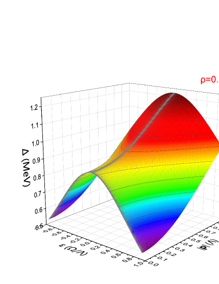
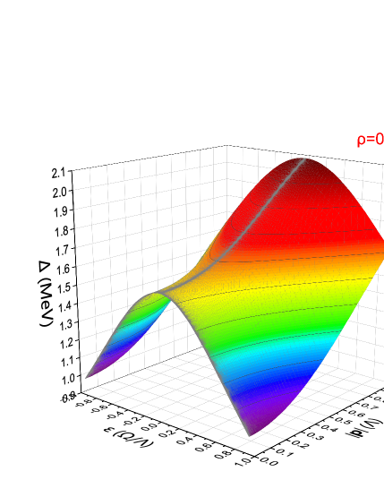
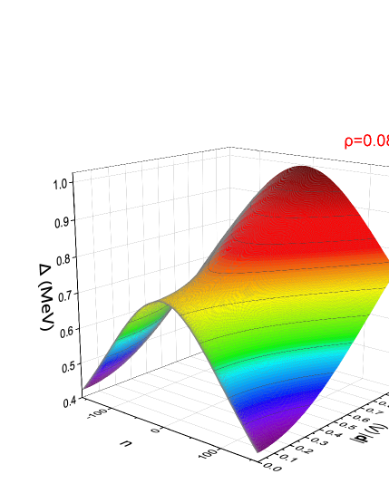
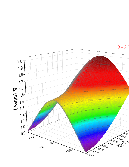
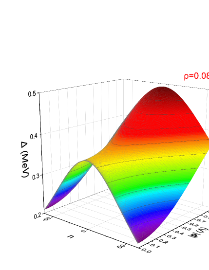
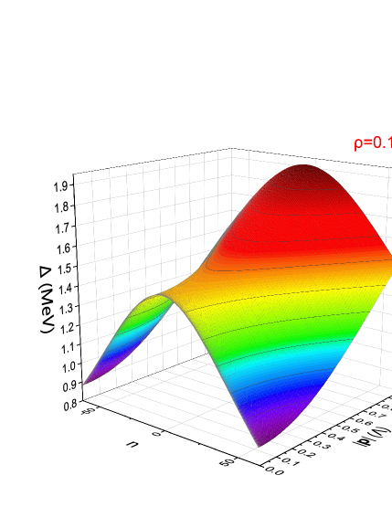
Figure 1: The energy-momentum dependence of the pairing gap $\Delta(\varepsilon,|\mathbf{p}|)$ obtained by solving the self-consistent integral equations of $\Delta_{s}(\varepsilon,|\mathbf{p}|)$ and $A_{0}(\varepsilon,|\mathbf{p}|)$. We choose six different set of tuning parameters $(\rho,T)$. Here and also in Fig. 2, we consider two representative densities: $\rho=0.08\rho_{0}$ and $\rho=0.1\rho_{0}$. The label $n$ denotes the neutron frequency $\varepsilon_{n}=(2n+1)\pi T$ in the case of finite $T$.

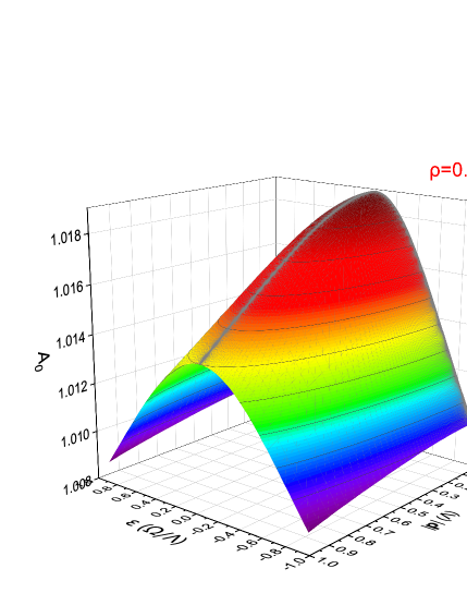
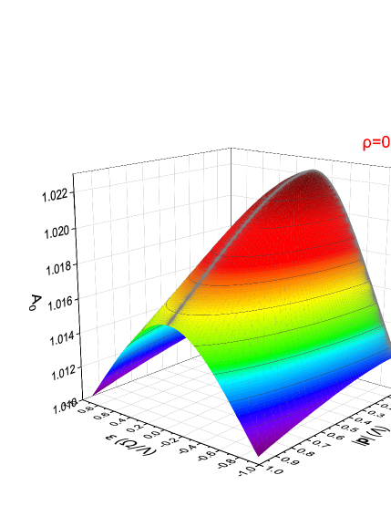
Figure 2: The energy-momentum dependence of the renormalization function $A_{0}(\varepsilon,|\mathbf{p}|)$ at zero temperature.

Next we move to calculate the critical values of $\rho_{c}$ and $T_{c}$. Such calculations are technically difficult because the iteration time needed to solve the coupled integral equations increases dramatically as the critical point is approached. In order to make numerics simpler, we now set $A_{0}(\varepsilon,|\mathbf{p}|)=1$ and solve solely the equation of $\Delta_{s}(\varepsilon,|\mathbf{p}|)$. According to our numerical results, it is more favorable to realize the neutron superfluid at higher densities and lower temperatures. In Fig. 4, a global phase diagram is plotted in the plane spanned by the normalized density $\rho/\rho_{0}$ and the temperature $T$. There is a critical line between the superfluid phase and the normal, Fermi liquid phase.

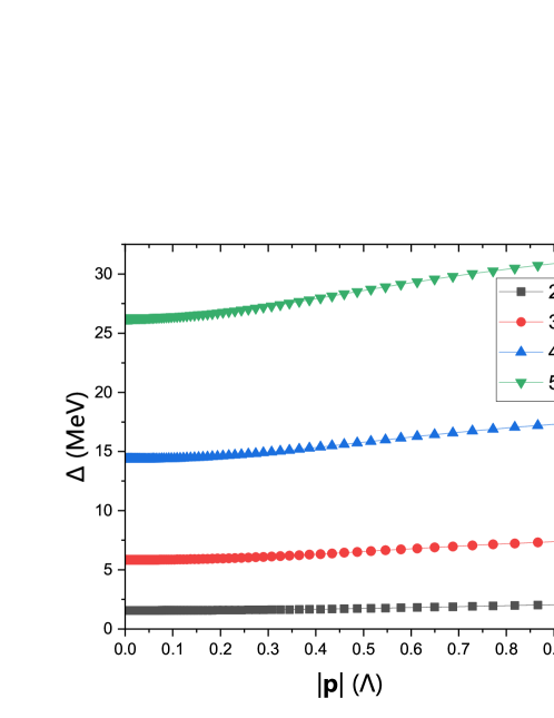
Figure 3: The momentum dependence of the pairing gap $\Delta$ at zero frequency for different values of ultraviolet cutoff $\Lambda$. The neutron density is $\rho=0.1\rho_{0}$.

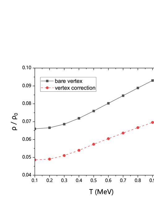
Figure 4: Global phase diagram of the low-density region of neutron matter on the temperature-density ($T$-$\rho$) plane obtained with (dashed line) and without (solid line) the contribution of one-loop vertex correction. Here, the density is normalized by saturation density $\rho_{0}$. The superfluid phase (upper left corner) and the normal phase (lower right corner) are separated by a critical line. It is clear that the inclusion of one-loop vertex correction can substantially alter the critical line, to be discussed in Sec. V.

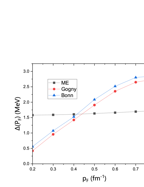
Figure 5: The ${}^{1}S_{0}$-wave neutron pairing gap $\Delta$ as a function of Fermi momentum $p_{F}$ obtained under three different approximations: ME-level, BCS-level based on Gogny force (data are taken from Refs. Kucharek89 ; Kucharek91 ; Furtado22 in the case of $D1$), and BCS-level based on relativistic Bonn potential (data are taken from Ref. Serra01 in the case of version B).

It is now useful to make a comparison between our results and some previous results on the pairing gap. The ${}^{1}S_{0}$-wave superfluid pairing gap $\Delta$ has been previously calculated at the BCS mean-field level based on a non-relativistic Gogny force $D1$ Kucharek89 ; Kucharek91 ; Furtado22 and also on a relativistic Bonn potential (so-called version B) Serra01 . Since both the long-range attraction and short-range repulsion are incorporated in the phenomenological Gogny force and Bonn potential, the gap obtained in these calculations exhibits a non-monotonic $p_{F}$ dependence. It was found Kucharek89 ; Kucharek91 ; Furtado22 ; Serra01 that $\Delta(p_{F})$ first increases with growing $p_{F}$ and then decreases with growing $p_{F}$ once $p_{F}$ exceeds roughly $0.8\mathrm{fm}^{-1}$, which corresponds to $\rho\approx 0.1\rho_{0}$. In Fig. 5, we compare the $p_{F}$-dependence of $\Delta$ obtained by solving the ME equations (34) and (35) with the BCS-level results obtained based on the Gogny force Kucharek89 ; Kucharek91 ; Furtado22 and the Bonn potential Serra01 within the range of $0.2\mathrm{fm}^{-1}\leq p_{F}\leq 0.8\mathrm{fm}^{-1}$. The Gogny result and Bonn result are quite similar to each other, but these two results are substantially different from our ME-level result. The Gogny force and the Bonn potential are determined by fitting with experimental data of scattering phase shifts and thus are more realistic than our $\pi N$ model. However, the BCS mean-field treatment has a serious limitation: it is carried out by using instantaneous nucleon-nucleon potentials and entirely ignores the time-dependence of nucleon-nucleon interaction and the Landau damping effects of neutrons. From the extensive theoretical studies on phonon-mediated superconductors Scalapino , we already know that the isotopic effect (the relation between superconducting $T_{c}$ and isotopic mass) of many metal and alloy superconductors could be well understood only after the retardation of electron-phonon interaction and the electron damping are properly considered. In the case of neutron superfluid, we believe that the retardation of neutron-meson interaction and the neutron damping are also important and should not be neglected. Unfortunately, it is difficult to handle these two effects properly within the framework of BCS mean-field theory. In comparison, our ME-level calculations take these two effects into account in a self-consistent manner. The limitation of our present work is that our results become invalid once $p_{F}$ is larger than $0.8\mathrm{fm}^{-1}$ (equivalent to $\rho>0.1\rho_{0}$) due to the presence of only one type of meson. In order to investigate the superfluid transition at higher densities, we will include other types of mesons, including $\sigma$, $\omega$, and $\rho$, in a forthcoming ME-level study.

The one-boson-exchange potential is widely used to study two-nucleon system, nuclear matter, and finite nuclei Erkelenz69 ; Erkelenz74 ; Holinde87 . The retardation effect could be partly considered by adding an energy term to the meson propagator by hands. In principle, one could use such a potential Erkelenz71 ; Holinde72 to derive a BCS-level gap equation to study superfluid transition. The main merit of this approach that it contains the contributions from several sorts of mesons, such as $\pi$, $\rho$, $\delta$, and $\omega$. However, in this approach only the on-shell processes are included, since the meson energy is defined by the difference $\omega=E_{\mathbf{p}^{\prime}}-E_{\mathbf{p}}$, where $E_{\mathbf{p}}=\sqrt{\mathbf{p}^{2}+M_{N}^{2}}$ is the neutron energy. Moreover, as demonstrated in Ref. Holinde87 , it appears that ignoring the energy term in the meson propagator is more suitable than keeping it. Actually, the nucleon-nucleon potential $V(\mathbf{p},\mathbf{p}^{\prime})$ and the $R$-matrix $R(\mathbf{p},\mathbf{p}^{\prime})$ used to calculate various quantities Erkelenz69 ; Erkelenz74 ; Holinde87 ; Erkelenz71 ; Holinde72 depend solely on momenta. As a result, the BCS gap equation derived from such potentials is energy independent, indicating that the retardation effect is not well treated. Furthermore, the neutron damping is still not incorporated in such an equation.

V Impact of lowest order vertex correction

The calculations of Sec. IV are based on the approximation of neglecting all the vertex corrections. Such an approximation, usually phrased as Migdal theorem Migdal ; Scalapino ; Fernandes in the condensed-matter community, has been broadly adopted in previous ME studies. The Migdal theorem is believed to be well justified in the case of weak electron-phonon interactions in ordinary metals with a large Fermi surface Migdal ; Scalapino ; Fernandes . In this section, we examine whether such a theorem is applicable in the $\pi N$ model.

To determine the importance of the electron-phonon vertex corrections, Migdal Migdal calculated the lowest order vertex correction, which is represented by the one-loop diagram shown in Fig. 6. For ordinary acoustic phonons, there is a characteristic Debye frequency $\omega_{D}$ that serves as an upper cutoff of phonon frequencies. This allows one to retain solely the contributions from the fixed frequency $\omega_{D}$. Making use of such an approximation, Migdal Migdal found that the one-loop vertex correction is proportional to $\sim\lambda\omega_{D}/E_{F}$. For ordinary metals, $\lambda\ll 1$ and $E_{F}\gg\omega_{D}$. In some element metals Fernandes , including Hg, Pb, and Al, the ratio $\omega_{D}/E_{F}$ is as small as $\sim 10^{-2}$. It is absolutely safe to omit all the electron-phonon vertex corrections for these systems. However, the $\pi N$ model is very different from electron-phonon systems. First, as aforementioned the coupling constant $f_{\pi}\approx 1.0$. Apparently, the $\pi N$ interaction is much stronger than electron-phonon interactions. Second, the $\pi N$ interacting system does not have such a characteristic energy scale as Debye frequency. It appears that the $\pi N$ vertex corrections cannot be suppressed by any small parameter.

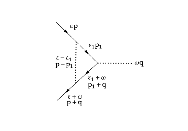
Figure 6: The Feynman diagram of one-loop vertex correction. The solid line represents the free fermion (electron or neutron) propagator and the dotted line represents the free boson (phonon or $\pi^{0}$) propagator.

Now we make a more quantitative analysis of the one-loop vertex correction to $\pi N$ interaction, following the strategy of Migdal Migdal . To avoid unnecessary formal complications, we do not utilize the Nambu spinor but turn to consider the Lagrangian density given by Eq. (12). The one-loop $\pi N$ vertex correction can be expressed as

$$\Gamma_{1} \propto \left(\frac{f_{\pi}}{m_{\pi}}\right)\left(\bm{\sigma}\cdot\mathbf{q}\right)\left(\frac{f_{\pi}}{m_{\pi}}\right)^{2}\int\frac{d\varepsilon_{1}d^{3}\mathbf{p_{1}}}{(2\pi)^{4}}\left[\bm{\sigma}\cdot\left(\mathbf{p-p_{1}}\right)\right]\left[\bm{\sigma}\cdot\left(\mathbf{p-p_{1}}\right)\right]$$ (36)

$$\times D_{0}(\varepsilon-\varepsilon_{1},\mathbf{p-p_{1}})G_{0}(\varepsilon_{1},\mathbf{p_{1}})G_{0}(\varepsilon_{1}+\omega,\mathbf{p_{1}+q})$$

$$= -\left(\frac{f_{\pi}}{m_{\pi}}\right)\left(\bm{\sigma}\cdot\mathbf{q}\right)\left(\frac{f_{\pi}}{m_{\pi}}\right)^{2}\int\frac{d\varepsilon_{1}d^{3}\mathbf{p_{1}}}{(2\pi)^{4}}$$

$$\times\frac{\left(\mathbf{p-p_{1}}\right)^{2}}{\left((\varepsilon-\varepsilon_{1})^{2}+(\mathbf{p-p_{1}})^{2}+m^{2}_{\pi}\right)\left(i\varepsilon_{1}-\xi_{\mathbf{p_{1}}}\right)\left(i(\varepsilon_{1}+\omega)-\xi_{\mathbf{p_{1}+q}}\right)}.$$

Here, the free fermion and boson propagators are given by $G_{0}(\varepsilon,\mathbf{p})=\frac{1}{i\varepsilon-\xi_{\mathbf{p}}}$ and $D_{0}(\omega,\mathbf{q})=-\frac{1}{\omega^{2}+\mathbf{q}^{2}+m^{2}_{\pi}}$, respectively.

The importance of one-loop vertex correction can be characterized by the ratio $\Gamma_{1}/\Gamma_{0}$, where

$$\Gamma_{0}\sim\left(\frac{f_{\pi}}{m_{\pi}}\right)\left(\bm{\sigma}\cdot\mathbf{q}\right)$$ (37)

is the bare vertex. This ratio has the following expression

$$\frac{\Gamma_{1}}{\Gamma_{0}}\propto-\left(\frac{f_{\pi}}{m_{\pi}}\right)^{2}\int\frac{d\varepsilon_{1}d^{3}\mathbf{p_{1}}}{(2\pi)^{4}}\frac{\left(\mathbf{p-p_{1}}\right)^{2}}{\left((\varepsilon-\varepsilon_{1})^{2}+(\mathbf{p-p_{1}})^{2}+m^{2}_{\pi}\right)\left(i\varepsilon_{1}-\xi_{\mathbf{p_{1}}}\right)\left(i\left(\varepsilon_{1}+\omega\right)-\xi_{\mathbf{p_{1}+q}}\right)},$$ (38)

which can be further written as

$$\frac{\Gamma_{1}}{\Gamma_{0}}\propto\left(\frac{f_{\pi}}{m_{\pi}}\right)^{2}\int\frac{d\varepsilon_{1}|\mathbf{p_{1}}|^{2}d|\mathbf{p_{1}}|dz}{(2\pi)^{3}}\frac{\left(|\mathbf{p}|^{2}-2|\mathbf{p}||\mathbf{p_{1}}|z+|\mathbf{p_{1}}|^{2}\right)\left(\varepsilon_{1}\left(\varepsilon_{1}+\omega\right)-i\varepsilon_{1}\xi_{\mathbf{p_{1}}}-i\left(\varepsilon_{1}+\omega\right)\xi_{\mathbf{p_{1}+q}}-\xi_{\mathbf{p_{1}}}\xi_{\mathbf{p_{1}+q}}\right)}{\left((\varepsilon-\varepsilon_{1})^{2}+(|\mathbf{p}|^{2}-2|\mathbf{p}||\mathbf{p_{1}}|z+|\mathbf{p_{1}}|^{2})+m^{2}_{\pi}\right)\left(\varepsilon^{2}_{1}+\xi^{2}_{\mathbf{p_{1}}}\right)\left(\left(\varepsilon_{1}+\omega\right)^{2}+\xi^{2}_{\mathbf{p_{1}+q}}\right)}.$$

Different from electron-phonon interacting systems, there is not any peculiar energy scale that could be adopted to carry out approximate analytical computations Migdal . Thus the method used by Migdal Migdal cannot be applied to compute the above integral. Below we calculate this integral as follows. An important property of neutron matter is that only the neutrons excited around the Fermi surface contribute to various physical quantities. Based on this property, we assume that the two external neutron momenta of the triangle diagram shown in Fig. 6 are both located at the Fermi surface, i.e., $|\mathbf{p}|=|\mathbf{p+q}|=p_{F}$. The two external frequencies are taken as $\varepsilon=\varepsilon+\omega=0$. Under such approximations, we set $\varepsilon=\omega=0$ and $|\mathbf{q}|\in[0,2p_{F}]$. For simplicity, we suppose that $|\mathbf{q}|=p_{F}$. We have verified that the results are not visibly changed if $|\mathbf{q}|$ takes other values around $p_{F}$. Now the ratio $\Gamma_{1}/\Gamma_{0}$ is simplified to

$$\frac{\Gamma_{1}}{\Gamma_{0}} \approx \left(\frac{f_{\pi}}{m_{\pi}}\right)^{2}\int\frac{d\varepsilon_{1}|\mathbf{p_{1}}|^{2}d|\mathbf{p_{1}}|dz}{(2\pi)^{3}}\frac{\left(p^{2}_{F}-2p_{F}|\mathbf{p_{1}}|z+|\mathbf{p_{1}}|^{2}\right)\left(\varepsilon^{2}_{1}-i\varepsilon_{1}\left(\xi_{\mathbf{p_{1}}}+\xi_{\mathbf{p_{1}}+p_{F}}\right)-\xi_{\mathbf{p_{1}}}\xi_{\mathbf{p_{1}}+p_{F}}\right)}{\left(\varepsilon_{1}^{2}+(p^{2}_{F}-2p_{F}|\mathbf{p_{1}}|z+|\mathbf{p_{1}}|^{2})+m^{2}_{\pi}\right)\left(\varepsilon^{2}_{1}+\xi^{2}_{\mathbf{p_{1}}}\right)\left(\varepsilon^{2}_{1}+\xi^{2}_{\mathbf{p_{1}}+p_{F}}\right)},$$

$$= \left(\frac{f_{\pi}}{m_{\pi}}\right)^{2}\int^{\Omega}_{-\Omega}\frac{d\varepsilon_{1}}{2\pi}\int^{\Lambda}_{0}\frac{|\mathbf{p_{1}}|^{2}d|\mathbf{p_{1}}|}{2\pi}\int^{1}_{-1}\frac{dz}{2\pi}\frac{\left(p^{2}_{F}-2p_{F}|\mathbf{p_{1}}|z+|\mathbf{p_{1}}|^{2}\right)\left(\varepsilon^{2}_{1}-\xi_{\mathbf{p_{1}}}\xi_{\mathbf{p_{1}}+p_{F}}\right)}{\left(\varepsilon_{1}^{2}+(p^{2}_{F}-2p_{F}|\mathbf{p_{1}}|z+|\mathbf{p_{1}}|^{2})+m^{2}_{\pi}\right)\left(\varepsilon^{2}_{1}+\xi^{2}_{\mathbf{p_{1}}}\right)\left(\varepsilon^{2}_{1}+\xi^{2}_{\mathbf{p_{1}}+p_{F}}\right)}.$$

This integral can be numerically computed. The numerical results are presented in Fig. 7. Apparently, the magnitude of the ratio $\Gamma_{1}/\Gamma_{0}$ depends strongly on the neutron density $\rho$. It is remarkable that the vertex correction is not negligible even at very low densities. For instance, we find that $\Gamma_{1}/\Gamma_{0}\approx 0.179$ at $\rho=0.05\rho_{0}$ and $\Gamma_{1}/\Gamma_{0}\approx 0.240$ at $\rho=0.1\rho_{0}$. A clear indication is that the contributions from vertex corrections cannot be simply neglected.

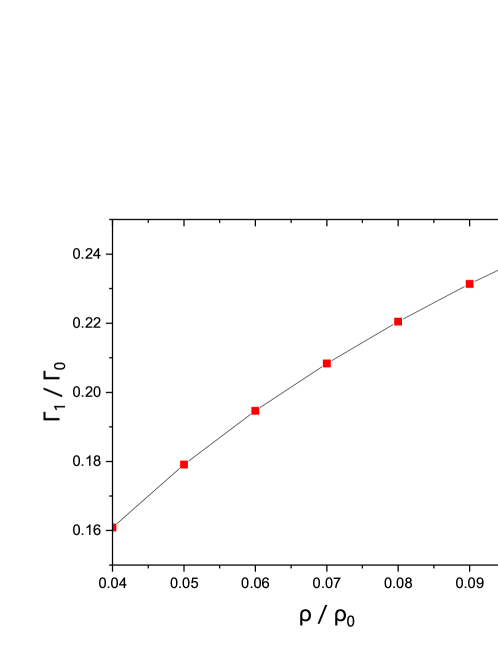
Figure 7: The ratio between one-loop vertex correction and bare vertex as a function of the relative neutron density $\rho/\rho_{0}$. The one-loop vertex correction becomes more important as the neutron density increases.

It is necessary to estimate to what extend the values of $T_{c}$ and $\rho_{c}$ are modified by the one-loop vertex correction. For simplicity, we suppose that the contribution of one-loop vertex correction can be effectively taken into account by replacing the bare parameter $\Gamma_{0}$ with $\Gamma_{0}+\Gamma_{1}$. Then we numerically solve the coupled equations of $A_{0}(\varepsilon_{n},|\mathbf{p}|)$ and $\Delta_{s}(\varepsilon_{n},|\mathbf{p}|)$ given by Eqs.(34-35) by making use of the new parameter $\Gamma_{0}+\Gamma_{1}$. In Fig. 4, we compare the critical line obtained under ME (bare vertex) approximation to that obtained by including the one-loop vertex correction. Obviously, the one-loop vertex correction makes significant contributions to both $\rho_{c}$ and $T_{c}$. We thus conclude that the ME theorem is invalid in the present model and the widely used ME theory is not a quantitatively reliable framework for the theoretical description of the pion-mediated superfluid transition.

VI Summary and Discussion

In summary, we apply the non-perturbative DS equation approach to study the superfluid transition driven by the pion-mediated Cooper pairing of neutrons. Based on a non-relativistic model of the interaction between neutrons and $\pi^{0}$-mesons, we derive the self-consistent integral equations of the renormalization function $A_{0}(p)$ and the pairing function $\Delta_{s}(p)$. After solving these two equations under the bare vertex approximation, we obtained the energy-momentum dependence of these two functions, extracted the critical temperature $T_{c}$ and the critical density $\rho_{c}$, and also plotted a global phased diagram on $T$-$\rho$ plane. Then we went beyond bare vertex approximation and incorporated the contributions of one-loop vertex correction into the equations of $A_{0}(p)$ and $\Delta_{s}(p)$. We re-solved these new equations and show that both $\rho_{c}$ and $T_{c}$ are significantly altered by the vertex correction, implying the invalidity of bare vertex approximation.

Our theoretical analysis need to be improved in three aspects. First of all, it is certainly not sufficient to consider only the one-loop vertex correction. Higher order vertex corrections should be taken into account. As discussed in the last paragraph of Sec. III, the approach developed in Refs. Liu21 ; Pan21 cannot be directly applied to precisely determine the full vertex function for the $\pi N$ model. Nevertheless, we find it still possible to properly generalize this approach to incorporate the contributions of higher order vertex corrections. This work is in progress and will be presented elsewhere Pan22 . Furthermore, our model does not have any self-interaction term of $\phi_{0}$ field. It would be interesting to examine the influence of such an term as $\phi_{0}^{4}$ on the superfluid transition. Another problem of our present work is that the $\pi N$ model describes only the low density region with $\rho/\rho_{0}\leq 0.1$ and does not provide an adequate description of realistic neutron stars. This is because exchanging pions only produces a long-range attraction needed to form Cooper pairs but is not capable of generating a short-range repulsion. For this reason, the pairing gap shown in Fig. 5 increases monotonously with growing density $\rho$ within the range $\rho/\rho_{0}\leq 0.1$. In the high density region (with $\rho/\rho_{0}>0.1$) where both long-range attraction and short-range repulsion are important, the gap should reach a maximum with growing $\rho$ and then tend to decrease as $\rho$ further grows. Although BCS treatment neglects some important effects, the phenomenological potential $V(r)$ used in BCS calculations does include both the attraction and repulsion. Thus, the pairing gap obtained by BCS calculations exhibits a maximum at certain neutron density Lombardoreview ; Sedrakian19 . To study the neutron superfluid in the high density region with $\rho>0.1\rho_{0}$, we should couple neutrons to other mesons, such as $\sigma$-meson, $\omega$-meson, and $\rho$-meson. Such an extended model would be more realistic, but formally much more complicated Walecka ; Glendenningbook . In a future project, we will generalize the DS equation analysis to treat the multiple neutron-meson couplings and to study both the ${}^{1}S_{0}$-wave and ${}^{3}PF_{2}$-wave Cooper pairing instabilities within a broader range of neutron density $\rho$.

Appendix A Dyson-Schwinger equation of neutron propagator

One can derive rigorously the complete set of DS integral equations of all the $n$-point correlation functions on the basis of the Lagrangian of $\pi N$ interaction. Here we only provide the derivational details that lead to the DS equation of neutron propagator $G(p)$. Other DS equations can be derived in a similar way Itzykson ; Liu21 ; Pan21 .

Let us start from the following total Lagrangian density

$$\mathcal{L}_{T} = \frac{1}{2}\widetilde{\psi}_{n}^{{\dagger}}(x)\left[i\partial_{t}-\xi_{\partial_{\mathbf{x}}}\widehat{A}~{}\right]\widetilde{\psi}_{n}(x)+\frac{1}{2}\phi_{0}^{{\dagger}}(x)\mathbb{D}_{\phi_{0}}\phi_{0}(x)$$ (41)

$$-\frac{i}{2}\frac{f_{\pi}}{m_{\pi}}\widetilde{\psi}_{n}^{{\dagger}}(x)\left[\widehat{C}\phi_{0}(x)\right]\widetilde{\psi}_{n}(x)$$

$$+J_{\phi_{0}}(x)\phi_{0}(x)+\eta^{{\dagger}}(x)\widetilde{\psi}_{n}(x)+\widetilde{\psi}_{n}^{{\dagger}}(x)\eta(x),$$

where $\mathbb{D}_{\phi_{0}}=-(\partial^{2}+m^{2}_{\pi})$, $J_{\phi_{0}}$, $\eta^{{{\dagger}}}$, and $\eta$ are external sources associated with $\phi_{0}$, $\widetilde{\psi}_{n}$, and $\widetilde{\psi}_{n}^{{{\dagger}}}$, respectively. For simplicity, we define the following notations

$$\widehat{A}=\lambda_{3}\otimes\sigma_{0},$$ (42)

$$\widehat{C}=i\partial_{i}\widehat{C}_{i}=i\partial_{x}\widehat{C}_{x}+i\partial_{y}\widehat{C}_{y}+i\partial_{z}\widehat{C}_{z}=i\partial_{x}\lambda_{0}\otimes\sigma_{1}+i\partial_{y}\lambda_{3}\otimes\sigma_{2}+i\partial_{z}\lambda_{0}\otimes\sigma_{3}.$$ (43)

To help the readers understand the calculational details, we first list some basic rules of functional integration to be used later. All the correlation functions are generated from three important quantities: the partition function $Z[J_{\phi_{0}},\eta^{{{\dagger}}},\eta]$, the generating functional $W[J_{\phi_{0}},\eta^{{{\dagger}}},\eta]$ and the generating functional $\Xi[\phi_{0},\widetilde{\psi}_{n},\widetilde{\psi}_{n}^{{\dagger}}]$. They are defined as follows:

$$Z\left[J_{\phi_{0}},\eta^{{{\dagger}}},\eta\right]=\int\mathcal{D}\phi_{0}\mathcal{D}\widetilde{\psi}_{n}^{{\dagger}}\mathcal{D}\widetilde{\psi}_{n}\exp{(i\int dtd^{3}\mathbf{x}\mathcal{L}_{T})},$$ (44)

$$W\left[J_{\phi_{0}},\eta^{{{\dagger}}},\eta\right]=-i\ln Z\left[J_{\phi_{0}},\eta^{{{\dagger}}},\eta\right],$$ (45)

$$\Xi\left[\phi_{0},\widetilde{\psi}_{n},\widetilde{\psi}_{n}^{{\dagger}}\right]=W\left[J_{\phi_{0}},\eta^{{{\dagger}}},\eta\right]-\int\left(J_{\phi_{0}}\phi_{0}+\eta^{{\dagger}}\widetilde{\psi}_{n}+\widetilde{\psi}_{n}^{{\dagger}}\eta\right).$$ (46)

The following identities will be frequently used:

$$\frac{\delta W}{\delta J_{\phi_{0}}}=\langle\phi_{0}\rangle,\qquad\frac{\delta W}{\delta\eta}=-\langle\widetilde{\psi}_{n}^{{\dagger}}\rangle,\qquad\frac{\delta W}{\delta\eta^{{\dagger}}}=\langle\widetilde{\psi}_{n}\rangle,$$ (47)

$$\frac{\delta\Xi}{\delta\phi_{0}}=-J_{\phi_{0}},\qquad\frac{\delta\Xi}{\delta\widetilde{\psi}_{n}}=\eta^{{\dagger}},\qquad\frac{\delta\Xi}{\delta\widetilde{\psi}_{n}^{{\dagger}}}=-\eta.$$ (48)

$W[J_{\phi_{0}},\eta^{{{\dagger}}},\eta]$ generates all the connected Green’s functions and $\Xi[\phi_{0},\widetilde{\psi}_{n},\widetilde{\psi}_{n}^{{\dagger}}]$ generates all the irreducible proper vertices of $\pi N$ coupling. For instance, the full neutron propagator $G(x-x^{\prime})$ and full pion propagator $F(x-x^{\prime})$ are given by

$$G(x-x^{\prime})\equiv-i\langle\widetilde{\psi}_{n}(x)\widetilde{\psi}^{\dagger}_{n}(x^{\prime})\rangle=\frac{\delta^{2}W}{\delta\eta^{\dagger}(x)\delta\eta(x^{\prime})},$$ (49)

$$F(x-x^{\prime})\equiv-i\langle\phi_{0}(x)\phi^{\dagger}_{0}(x^{\prime})\rangle=-\frac{\delta^{2}W}{\delta J_{\phi_{0}}(x)\delta J_{\phi_{0}}(x^{\prime})},$$ (50)

and the $three$-point correlation function $\langle\phi_{0}\widetilde{\psi}_{n}\widetilde{\psi}^{\dagger}_{n}\rangle$ is defined as follows:

$$\langle\phi_{0}\widetilde{\psi}_{n}\widetilde{\psi}^{\dagger}_{n}\rangle\equiv\frac{\delta^{3}W}{\delta J_{\phi_{0}}\delta\eta^{\dagger}\delta\eta}.$$ (51)

The following identity will also be frequently used:

$$\frac{\delta^{3}W}{\delta J_{\phi_{0}}\delta\eta^{\dagger}\delta\eta}=-FG\frac{\delta^{3}\Xi}{\delta\phi_{0}\delta\widetilde{\psi}_{n}^{{\dagger}}\delta\widetilde{\psi}_{n}}G.$$ (52)

Now we derive the DS equation of the full neutron propagator. The partition function $Z$ is invariant under an arbitrary infinitesimal variation of spinor field $\widetilde{\psi}_{n}^{{\dagger}}$, i.e.,

$$\int\mathcal{D}\phi_{0}\mathcal{D}\widetilde{\psi}_{n}^{{\dagger}}\mathcal{D}\widetilde{\psi}_{n}\frac{\delta}{i\delta\widetilde{\psi}_{n}^{{\dagger}}}\exp{(i\int dtd^{3}\mathbf{x}\mathcal{L}_{T})}=0.$$ (53)

It is easy to obtain

$$\langle\left(i\partial_{t}-\xi_{\partial_{\mathbf{x}}}\widehat{A}~{}\right)\widetilde{\psi}_{n}(x)-i\frac{f_{\pi}}{m_{\pi}}\left[\widehat{C}\phi_{0}(x)\right]\widetilde{\psi}_{n}(x)+2\eta(x)\rangle=0.$$ (54)

Using the relations given by Eq. (47), we re-write the above expression as

$$-2\eta(x) = \left(i\partial_{t}-\xi_{\partial_{\mathbf{x}}}\widehat{A}~{}\right)\frac{\delta W}{\delta\eta^{{\dagger}}(x)}-\frac{f_{\pi}}{m_{\pi}}\widehat{C}\frac{\delta^{2}W}{\delta J_{\phi_{0}}(x)\delta\eta^{{\dagger}}(x)}-i\frac{f_{\pi}}{m_{\pi}}\left(i\partial_{i}\frac{\delta W}{\delta J_{\phi_{0}}(x)}\right)\widehat{C}_{i}\frac{\delta W}{\delta\eta^{{\dagger}}(x)}.$$ (55)

The last term of the right-hand side (r.h.s.) vanishes upon removing sources and can be directly omitted. Performing functional derivative of both sides with respect to $\eta(x_{2})$ and using the identity (52) leads to

$$2\delta(x-x_{2}) = \left(i\partial_{t}-\xi_{\partial_{\mathbf{x}}}\widehat{A}~{}\right)\frac{\delta^{2}W}{\delta\eta^{{\dagger}}(x)\delta\eta(x_{2})}-\frac{f_{\pi}}{m_{\pi}}\widehat{C}\frac{\delta^{3}W}{\delta J_{\phi_{0}}(z)\delta\eta^{{\dagger}}(x)\delta\eta(x_{2})}$$ (56)

$$= \left(i\partial_{t}-\xi_{\partial_{\mathbf{x}}}\widehat{A}~{}\right)G(x-x_{2})$$

$$+\frac{f_{\pi}}{m_{\pi}}\int dx_{1}dx_{3}dx_{4}\widehat{C}F(x-x_{3})G(x-x_{1})\frac{\delta^{3}\Xi}{\delta\phi_{0}(x_{3})\delta\widetilde{\psi}_{n}^{{\dagger}}(x_{1})\delta\widetilde{\psi}_{n}(x_{4})}G(x_{4}-x_{2}).$$

This expression can be re-cast into

$$2G^{-1}(x-x_{2})=\left(i\partial_{t}-\xi_{\partial_{\mathbf{x}}}\widehat{A}~{}\right)\delta(x-x_{2})+\frac{f_{\pi}}{m_{\pi}}\int dx_{1}dx_{3}\widehat{C}F(x-x_{3})G(x-x_{1})\Gamma_{\mathrm{v}}(x_{3},x_{1},x_{2}),$$ (57)

where we have defined a truncated (without external legs) $\pi N$ interaction vertex function

$$\Gamma_{\mathrm{v}}(x_{3},x_{1},x_{2})=\frac{\delta^{3}\Xi}{\delta\phi_{0}(x_{3})\delta\widetilde{\psi}_{n}^{{\dagger}}(x_{1})\delta\widetilde{\psi}_{n}(x_{2})}.$$ (58)

The full neutron propagator, the full pion propagator and interaction vertex functions are Fourier transformed as

$$G(x-\xi_{1}) = \int\frac{d^{4}p}{(2\pi)^{4}}e^{-ip(x-\xi_{1})}G(p),$$ (59)

$$F(x-\xi_{2}) = \int\frac{d^{4}q}{(2\pi)^{4}}e^{-iq(x-\xi_{2})}F(q),$$ (60)

$$\Gamma_{\mathrm{v}}(\xi_{1}-x,x-\xi_{2}) = \int\frac{d^{4}qd^{4}p}{(2\pi)^{8}}e^{-i(p+q)(\xi_{1}-x)-ip(x-\xi_{2})}\Gamma_{\mathrm{v}}(q,p).$$ (61)

After making Fourier transformation Eqs. (59-61) to Eq. (57), we eventually obtain the following DS equation for the full neutron propagator:

$$G^{-1}(p)=G_{0}^{-1}(p)-\frac{1}{2}\frac{f_{\pi}}{m_{\pi}}\int\frac{d^{4}q}{(2\pi)^{4}}\widehat{C}_{1}G(p+q)F(q)\Gamma_{\mathrm{v}}(q,p),$$ (62)

where

$$\widehat{C}_{1} = q_{x}\lambda_{0}\otimes\sigma_{1}+q_{y}\lambda_{3}\otimes\sigma_{2}+q_{z}\lambda_{0}\otimes\sigma_{3}.$$ (63)

The DS equation of the full pion propagator can be derived in an analogous way. We will not give the derivational details and only present their final expression

$$F^{-1}(q)=F_{0}^{-1}(q)+\frac{1}{2}\frac{f_{\pi}}{m_{\pi}}\int\frac{d^{4}p}{(2\pi)^{4}}\mathrm{Tr}\left[\widehat{C}_{1}G(p+q)\Gamma_{\mathrm{v}}(q,p)G(q)\right].$$ (64)

We next derive an exact relation that connects $F(q)$ and $F_{0}(q)$ with $\Gamma_{\mathrm{v}}(q,p)$. It is clearly true that $Z$ is not changed by infinitesimal variations of pion field $\phi_{0}(x)$, which indicates that

$$\langle\mathbb{D}_{\phi_{0}}\phi_{0}(x)+i\frac{1}{2}\frac{f_{\pi}}{m_{\pi}}\left[i\partial_{i}\widetilde{\psi}_{n}^{{\dagger}}(x)\widehat{C}_{i}\widetilde{\psi}_{n}(x)\right]+J_{\phi_{0}}(x)\rangle=0.$$ (65)

This equation can be converted to

$$-i\frac{1}{2}\frac{f_{\pi}}{m_{\pi}}\langle\left[i\partial_{i}\widetilde{\psi}_{n}^{{\dagger}}(x)\widehat{C}_{i}\widetilde{\psi}_{n}(x)\right]\rangle=\mathbb{D}_{\phi_{0}}\frac{\delta W}{\delta J_{\phi_{0}}(x)}+J(x),$$ (66)

which, after taking the functional derivative with respect to $\eta^{{\dagger}}$ and $\eta$ in order, leads to

$$\frac{\delta^{2}}{\delta\eta^{{\dagger}}(x_{1})\delta\eta(x_{2})}\langle\left[i\partial_{i}\widetilde{\psi}_{n}^{{\dagger}}(x)\widehat{C}_{i}\widetilde{\psi}_{n}(x)\right]\rangle$$ (67)

$$= \langle\left[i\partial_{i}\widetilde{\psi}_{n}^{{\dagger}}(x)\widehat{C}_{i}\widetilde{\psi}_{n}(x)\right]\widetilde{\psi}_{n}(x_{1})\widetilde{\psi}_{n}^{{\dagger}}(x_{2})\rangle$$

$$= \langle\left[i\partial_{x}\widetilde{\psi}_{n}^{{\dagger}}(x)\widehat{C}_{x}\widetilde{\psi}_{n}(x)+i\partial_{y}\widetilde{\psi}_{n}^{{\dagger}}(x)\widehat{C}_{y}\widetilde{\psi}_{n}(x)+i\partial_{z}\widetilde{\psi}_{n}^{{\dagger}}(x)\widehat{C}_{z}\widetilde{\psi}_{n}(x)\right]\widetilde{\psi_{n}}(x_{1})\widetilde{\psi}_{n}^{{\dagger}}(x_{2})\rangle$$

$$= i2\left(\frac{f_{\pi}}{m_{\pi}}\right)^{-1}\mathbb{D}_{\phi_{0}}\frac{\delta^{3}W}{\delta J_{\phi_{0}}(x)\delta\eta^{{\dagger}}(x_{1})\delta\eta(x_{2})}.$$

Making use of the three current vertex functions defined by Eq. (24) and the identity (52), we obtain the following exact relation

$$\int dx_{3}dx_{4}G(x_{1}-x_{3})\left[i\partial_{x}\Gamma_{\widehat{C}_{x}}(x,x_{3},x_{4})+i\partial_{y}\Gamma_{\widehat{C}_{y}}(x,x_{3},x_{4})+i\partial_{z}\Gamma_{\widehat{C}_{z}}(x,x_{3},x_{4})\right]G(x_{4}-x_{2})$$ (68)

$$= \int dx_{3}dx_{4}dx_{5}i2\left(\frac{f_{\pi}}{m_{\pi}}\right)^{-1}\mathbb{D}_{\phi_{0}}F(x-x_{5})G(x_{1}-x_{3})\Gamma_{\mathrm{v}}(x_{5},x_{3},x_{4})G(x_{4}-x_{2}).$$

The current vertex functions are Fourier transformed as

$$\Gamma_{\widehat{C}_{x,y,z}}(\xi_{1}-x,x-\xi_{2}) = \int\frac{d^{4}qd^{4}p}{(2\pi)^{8}}e^{-i(p+q)(\xi_{1}-x)-ip(x-\xi_{2})}\Gamma_{\widehat{C}_{x,y,z}}(q,p).$$ (69)

Making Fourier transformation to Eq. (68) gives rise to

$$i2\left(\frac{f_{\pi}}{m_{\pi}}\right)^{-1}F_{0}^{-1}(q)F(q)\Gamma_{\mathrm{v}}(q,p)=q_{x}\Gamma_{\widehat{C}_{x}}(q,p)+q_{y}\Gamma_{\widehat{C}_{y}}(q,p)+q_{z}\Gamma_{\widehat{C}_{z}}(q,p).$$ (70)

It is more convenient to re-write this relation as

$$F(q)\Gamma_{\mathrm{v}}(q,p)=-i\frac{1}{2}\frac{f_{\pi}}{m_{\pi}}F_{0}(q)\left[q_{x}\Gamma_{\widehat{C}_{x}}(q,p)+q_{y}\Gamma_{\widehat{C}_{y}}(q,p)+q_{z}\Gamma_{\widehat{C}_{z}}(q,p)\right].$$ (71)

This relation is used in Sec. III.