Chaotic Hedging with Iterated Integrals and Neural Networks

Abstract.

In this paper, we extend the Wiener-Ito chaos decomposition to the class of diffusion processes, whose drift and diffusion coefficient are of linear growth. By omitting the orthogonality in the chaos expansion, we are able to show that every $p$-integrable functional, for $p\in[1,\infty)$, can be represented as sum of iterated integrals of the underlying process. Using a truncated sum of this expansion and (possibly random) neural networks for the integrands, whose parameters are learned in a machine learning setting, we show that every financial derivative can be approximated arbitrarily well in the $L^{p}$-sense. Since the hedging strategy of the approximating option can be computed in closed form, we obtain an efficient algorithm that can replicate any integrable financial derivative with short runtime.

1. Introduction

We address the problem of pricing and hedging a financial derivative within a financial market consisting of $d\in\mathbb{N}$ risky assets, whose prices are modelled by a diffusion process with drift and diffusion coefficient of linear growth. This includes in particular affine and some polynomial diffusion processes (see [Duffie et al., 2000], [Cuchiero, 2011], and [Filipović and Larsson, 2016]). While in complete markets, every financial derivative can be perfectly replicated using one pricing measure, the hedging problem in incomplete markets needs to be addressed with an additional criteria, for example, “mean-variance hedging” (see e.g. [Duffie and Richardson, 1991], [Schweizer, 1992], and [Pham et al., 1998]), “super-replication” (see e.g. [El Karoui and Quenez, 1995], [Cvitanić et al., 1999], [Cheridito et al., 2005], and [Acciaio et al., 2016]), “quadratic hedging” (see e.g. [Schweizer, 1999] and [Pham, 2000]), or “utility indifference pricing and hedging” (see e.g. [Musiela and Zariphopoulou, 2004] and [Carmona, 2009]).

Our “chaotic hedging” approach solves the hedging problem by minimizing a given loss function and is therefore similar to the idea of “quadratic hedging”. The numerical algorithm relies on the so-called chaos expansion of a financial derivative, which can be seen as Taylor formula for random variables, and has been applied for option pricing (see [Lacoste, 1996] and [Lelong, 2018]) and for solving stochastic differential equations (SDEs) (see [Xiu and Karniadakis, 2002]). Moreover, by proving a universal approximation result for random neural networks, we are able to efficiently learn the financial payoff. We refer to other successful neural networks applications in finance (see e.g. [Han et al., 2018], [Bühler et al., 2019], [Sirignano and Cont, 2019], [Cuchiero et al., 2020], [Eckstein et al., 2020], [Eckstein et al., 2021], [Neufeld and Sester, 2022], [Neufeld et al., 2022], and [Schmocker, 2022]). Altogether, this paper introduces a fast two-step approximation of any sufficiently integrable financial derivative, by first using a truncation of its chaos expansion, and then learning (random) neural networks for each order of the expansion. The algorithm can be also applied to high-dimensional options and returns the hedging strategy of the approximation in closed form.

The main idea of this paper relies on the chaos expansion of a financial derivative. In the Brownian motion case, the so-called Wiener-Ito chaos decomposition (see [Ito, 1951, Theorem 4.2]) yields an expression for every square-integrable functional of the Brownian path as infinite sum of iterated integrals of the given Brownian motion. This was later extended to the compensated Poisson process (see [Ito, 1956, Theorem 2]) and Azéma martingales (see [Émery, 1989, Proposition 6]). Moreover, [Løkka, 2004], [Jamshidian, 2005], [Di Nunno et al., 2008], and [Di Tella and Engelbert, 2016a] proved the chaos expansion for particular martingales with independent increments. However, to the best of our knowledge, a chaos expansion with respect to a diffusion process with stochastic covariation and non-independent increments has not yet been established in the literature. Opposed to the classical Wiener-Ito chaos decomposition, we omit the orthogonality in the chaos expansion and use the direct sum (instead of the orthogonal sum) together with the so-called “time-space harmonic Hermite polynomials” in order to span the chaotic subspaces. Moreover, by extending the Kailath-Segall formula in [Segall and Kailath, 1976], we are able to express every $p$-integrable functionals, $p\in[1,\infty)$, as iterated integrals of the underlying diffusion process, which yields an analogue of the classical Wiener-Ito chaos decomposition in this more general setting with possible drift process.

It is well-known that whenever the underlying stochastic process is a Brownian motion, the chaos expansion can be used to obtain a martingale representation result, which ensures the existence of a hedging strategy for each square-integrable functional of the Brownian path, see e.g. [Karatzas and Shreve, 1998, Section 3.4]. This has been extended to the compensated Poisson process (see e.g. [Ikeda and Watanabe, 1989, Theorem II.6.7]), Azéma martingales (see [Émery, 1989]), and other martingales with independent increments (see [Nualart and Schoutens, 2000], [Løkka, 2004], [Davis, 2005], [Jamshidian, 2005], and [Di Tella and Engelbert, 2016b]). In our setting, we are able to retrieve a similar representation, but with respect to the diffusion process, which relies on the $L^{p}$-closedness of stochastic integrals (see [Grandits and Krawczyk, 1998] and [Delbaen et al., 1997]). This leads us in the martingale case (i.e. without drift) to a martingale representation result similar to [Soner et al., 2011, Theorem 6.5].

The machine learning application of this paper consists of learning the integrands of the iterated integrals in the chaos expansion. More precisely, we first approximate a financial derivative by truncating the infinite sum of iterated integrals from its chaos expansion, and then replace the deterministic integrands by neural networks. This provides us with a parametric family of financial derivatives, whose optimal coefficients can be learned by minimizing a loss function in the sense of “quadratic hedging”.

In addition, we extend our universal approximation result for financial derivatives to random neural networks with randomly initialized weights and biases, which is inspired by the works on extreme learning machines and random features (see e.g. [Huang et al., 2006], [Rahimi and Recht, 2007], [Grigoryeva and Ortega, 2018], [Gonon et al., 2022], and [Gonon, 2022]). In this case, the optimization procedure reduces to the training of the linear readout, which can be performed, e.g., by a simple linear regression. This can be solved within few minutes, also for high-dimensional financial derivatives.

Altogether, our “chaotic hedging” approach provides a “global” universal approximation result for financial derivatives by using the $\|\cdot\|_{L^{p}(\mathbb{P})}$-norm. This is more general than other universal approximation results for financial applications (see e.g. [Lyons et al., 2019], [Benth et al., 2022], [Lyons et al., 2020], [Acciaio et al., 2022], and [Cuchiero et al., 2022b]), where the approximation holds true on a compact subset of the sample path space. Other “global” universal approximation results have been found in [Király and Oberhauser, 2019], [Schmocker, 2022], and [Cuchiero et al., 2023]. However, in this paper, we exploit the chaos expansion of a given financial derivative to learn its hedging strategy.

1.1. Outline

In Section 2, we introduce the setting of this paper and provide the main theoretical results, including the chaos expansion, the corresponding (semi-) martingale representation result, and the theoretical approximation results for financial derivatives. Subsequently, we illustrate in Section 3 how these theoretical results can be applied to learn the hedging strategy of various options in different markets. Finally, all proofs of the theoretical results are given in Section 4.

1.2. Notation

As usual, $\mathbb{N}=\{1,2,...\}$ and $\mathbb{N}_{0}=\mathbb{N}\cup\{0\}$ denote the sets of natural numbers, whereas $\mathbb{R}$ and $\mathbb{C}$ represent the real and complex numbers (with complex unit $i:=\sqrt{-1}$), respectively, where $s\wedge t:=\min(s,t)$, for $s,t\in\mathbb{R}$. Moreover, $\mathbb{R}^{d}$ denotes the Euclidean space equipped with the norm $\|x\|=\sqrt{x_{1}^{2}+...+x_{d}^{2}}$, whereas $\mathbb{R}^{d\times l}$ represents the vector space of matrices $A=(a_{ij})_{i=1,...,d;\,j=1,...,l}$ equipped with the Frobenius norm $\|A\|_{F}=\left(\sum_{i=1}^{d}\sum_{j=1}^{l}|a_{ij}|^{2}\right)^{1/2}$. Hereby, $\mathbb{S}^{d}_{+}\subset\mathbb{R}^{d\times d}$ denotes the cone of symmetric non-negative definite matrices and $I_{d}\in\mathbb{S}^{d}_{+}$ represents the identity matrix.

In addition, for $S\subseteq\mathbb{R}^{k}$, with $k\in\mathbb{N}$, $\mathcal{B}(S)$ represents the Borel $\sigma$-algebra of $S$, whereas $C(S)$ denotes the space of continuous functions $f:S\rightarrow\mathbb{R}$. Furthermore, for $p\in[1,\infty)$ and $T>0$, we denote by $L^{p}([0,T],\mathcal{B}([0,T]),dt;\mathbb{R}^{d})$ the Banach space of $\mathcal{B}([0,T])/\mathcal{B}(\mathbb{R}^{d})$-measurable functions $f:[0,T]\rightarrow\mathbb{R}^{d}$ with finite norm $\|f\|_{L^{p}([0,T],\mathcal{B}([0,T]),dt;\mathbb{R}^{d})}:=\left(\int_{0}^{T}\|f(t)\|^{p}dt\right)^{1/p}$, whereas for $p=2$, the inner product $\langle f,g\rangle_{L^{2}([0,T],\mathcal{B}([0,T]),dt;\mathbb{R}^{d})}=\int_{0}^{T}f(t)^{\top}g(t)dt$ turns $L^{2}([0,T],\mathcal{B}([0,T]),dt;\mathbb{R}^{d})$ into a Hilbert space. Moreover, we abbreviate $L^{p}([0,T],\mathcal{B}([0,T]),dt):=L^{p}([0,T],\mathcal{B}([0,T]),dt;\mathbb{R})$.

2. Setting and Main Results

Throughout this paper, we consider a financial market with finite time horizon $T>0$ consisting of $d\in\mathbb{N}$ risky assets, whose vector of price processes follows a stochastic process $X=\left(X^{1}_{t},...,X^{d}_{t}\right)_{t\in[0,T]}^{\top}$ with continuous sample paths and values in a subset $E\subseteq\mathbb{R}^{d}$.

2.1. Setting

On a given probability space $(\Omega,\mathcal{A},\mathbb{P})$, we fix an $l$-dimensional Brownian motion $B=(B^{1}_{t},...,B^{l}_{t})^{\top}_{t\in[0,T]}$ endowed with the natural $\mathbb{P}$-augmented filtration $\mathbb{F}=(\mathcal{F}_{t})_{t\in[0,T]}$ generated by $B$ such that $\mathcal{F}_{T}=\mathcal{A}$, and let $b=(b_{1},...,b_{d})^{\top}:[0,T]\times E\rightarrow\mathbb{R}^{d}$ and $\sigma=(\sigma_{ij})_{i=1,...,d;\,j=1,...,l}:[0,T]\times E\rightarrow\mathbb{R}^{d\times l}$ be continuous. We assume that $X$ is an $E$-valued strong solution (see [Karatzas and Shreve, 1998, Definition 5.2.1]) of the stochastic differential equation (SDE) $dX_{t}=b(t,X_{t})dt+\sigma(t,X_{t})dB_{t}$, with $E\subseteq\mathbb{R}^{d}$, i.e. $X$ is $\mathbb{F}$-adapted, and for every $i=1,...,d$ and $t\in[0,T]$, it holds $\mathbb{P}$-a.s. that

$$X^{i}_{t}=X^{i}_{0}+\int_{0}^{t}b_{i}(s,X_{s})ds+\sum_{j=1}^{l}\int_{0}^{t}\sigma_{ij}(s,X_{s})dB^{j}_{s},\quad\quad X_{0}\in E,$$ (1)

where $\int_{0}^{T}\left(\|b(s,X_{s})\|+\|\sigma(s,X_{s})\|_{F}^{2}\right)ds<\infty$, $\mathbb{P}$-a.s.

Definition 2.1.

An $E$-valued strong solution of (1) is called a (time-inhomogeneous) diffusion process $X$ on $E$ with drift coefficient $b:[0,T]\times E\rightarrow\mathbb{R}^{d}$ and diffusion coefficient $a:[0,T]\times E\rightarrow\mathbb{S}^{d}_{+}$ defined by

$$a(t,x)=\sigma(t,x)\sigma(t,x)^{\top},$$

for $(t,x)\in[0,T]\times E$. Moreover, we say that the drift $b:[0,T]\times E\rightarrow\mathbb{R}^{d}$ and diffusion coefficient $a:[0,T]\times E\rightarrow\mathbb{S}^{d}_{+}$ (shortly “coefficients”) are of linear growth if there exists some $C_{L}>0$ such that

$$\|b(t,x)\|+\|a(t,x)\|_{F}\leq C_{L}\left(1+\|x\|\right),$$

for all $(t,x)\in[0,T]\times E$.

Remark 2.2.

By [Karatzas and Shreve, 1998, Thereom 5.2.9], (1) admits a strong solution if, e.g., $b:[0,T]\times E\rightarrow\mathbb{R}^{d}$ and $\sigma:[0,T]\times E\rightarrow\mathbb{R}^{d\times l}$ satisfy a Lipschitz and linear growth condition, i.e. there exists a constant $C_{1}>0$ such that for every $x,y\in E$ and $t\in[0,T]$, it holds that

$$\|b(t,x)-b(t,y)\|+\|\sigma(t,x)-\sigma(t,y)\|_{F} \leq C_{1}\|x-y\|,$$

$$\|b(t,x)\|+\|\sigma(t,x)\|_{F} \leq C_{1}(1+\|x\|).$$

Moreover, (1) admits by the Yamada conditions in [Yamada and Watanabe, 1971] a strong solution (see also [Ikeda and Watanabe, 1989, Theorem IV.3.2] and [Altay and Schmock, 2016, Theorem 2.1 & Remark 2.7] for $d,m\geq 2$) if there exists $\gamma>0$ and $G,\kappa,\eta:[0,\gamma]\rightarrow[0,\infty)$ with $G(0)=\kappa(0)=0$, $G:[0,\gamma]\rightarrow[0,\infty)$ non-decreasing, concave, and continuous, $\eta:[0,\gamma]\rightarrow[0,\infty)$ non-decreasing, $\eta(u)>0$ for all $u\in(0,\gamma]$, $\int_{0}^{\gamma}\frac{1}{G(u)}du=\int_{0}^{\gamma}\frac{1}{\eta(u)^{2}}du=\infty$, and $G(u)\geq\kappa(u)+\frac{d-1}{2u}\eta(u)^{2}$ for all $u\in(0,\gamma]$, such that for every $x,y\in E$ with $\|x-y\|\leq\gamma$ and $t\in[0,T]$, it holds that

$$\|b(t,x)-b(t,y)\|\leq\kappa\left(\|x-y\|\right)\quad\text{and}\quad\|\sigma(t,x)-\sigma(t,y)\|_{F}\leq\eta\left(\|x-y\|\right).$$

Example 2.3 (Polynomial Diffusions).

For $d=m=1$, let $B=(B_{t})_{t\in[0,T]}$ be a one-dimensional Brownian motion and let $X$ be an $E$-valued solution of (1) with time-homogeneous drift $b(x)=\beta_{0}+\beta_{1}x$ and diffusion coefficient $a(x)=\alpha_{0}+\alpha_{1}x+\alpha_{2}x^{2}$, i.e.

$$dX_{t}=(\beta_{0}+\beta_{1}X_{t})dt+\sqrt{\alpha_{0}+\alpha_{1}X_{t}+\alpha_{2}X_{t}^{2}}dB_{t},$$ (2)

for $t\in[0,T]$. Hereby, the state space $E\subseteq\mathbb{R}$ depends on $\beta_{0},\beta_{1},\alpha_{0},\alpha_{1},\alpha_{2}\in\mathbb{R}$, which we require to satisfy $\alpha_{0}+\alpha_{1}x+\alpha_{2}x^{2}\geq 0$, for all $x\in E$. For $\kappa(u)=|\beta_{1}|u$ and $\eta(u)=\sqrt{\left(|\alpha_{1}|+2\gamma|\alpha_{2}|\right)u}$, with $\gamma>0$, it follows by choosing $G(u):=\kappa(u)$ (see [Altay and Schmock, 2016, Remark 2.7]) and inserting the inequality $|\sqrt{x}-\sqrt{y}|\leq\sqrt{|x-y|}$ for any $x,y\geq 0$, that

$$|b(x)-b(y)| =|(\beta_{0}+\beta_{1}x)-(\beta_{0}+\beta_{1}y)|\leq|\beta_{1}||x-y|=\kappa(|x-y|),$$

$$\left|\sqrt{a(x)}-\sqrt{a(y)}\right| =\left|\sqrt{\alpha_{0}+\alpha_{1}x+\alpha_{2}x^{2}}-\sqrt{\alpha_{0}+\alpha_{1}y+\alpha_{2}y^{2}}\right|$$

$$\leq\sqrt{\left|\alpha_{1}(x-y)+\alpha_{2}\left(x^{2}-y^{2}\right)\right|}$$

$$\leq\sqrt{|\alpha_{1}||x-y|+2\gamma|\alpha_{2}||x-y|}=\eta(|x-y|).$$

Hence, (2) admits by Remark 2.2 a strong solution, which shows that $X$ is a diffusion process, called a polynomial diffusion in the sense of [Filipović and Larsson, 2016, Definition 2.1]. Moreover, in the case of vanishing drift (i.e. $\beta_{0}=\beta_{1}=0$), there are in particular three relevant cases:

$$E=\mathbb{R} \text{with }\alpha_{0}>0\text{, }\alpha_{1}=0\text{ and }\alpha_{2}\geq 0,$$ e.g. Brownian motion (BM), (3a)

$$E=[0,\infty) \text{with }\alpha_{0}=0\text{ and }\alpha_{1},\alpha_{2}\geq 0, \text{e.g. geometric BM (GBM)},$$ (3b)

$$E=[0,1] \text{with }\alpha_{0}=0\text{ and }\alpha_{1}=-\alpha_{2},$$ e.g. Jacobi process. (3c)

If $\alpha_{2}=0$ or $E$ is compact (e.g. (3c)), the diffusion coefficient $a$ is of linear growth. Moreover, conditional moments $\mathbb{E}\left[X_{t}^{k}\big{|}\mathcal{F}_{s}\right]$ and higher order correlators $\mathbb{E}\left[X_{t_{1}}^{k_{1}}\cdots X_{t_{n}}^{k_{n}}\big{|}\mathcal{F}_{s}\right]$ can be computed with [Filipović and Larsson, 2016, Theorem 3.1] and [Benth and Lavagnini, 2021, Theorem 4.5], respectively.

In the remaining part of this section, we prove that an $E$-valued time-inhomogeneous diffusion process with drift $b:[0,T]\times E\rightarrow\mathbb{R}^{d}$ and diffusion coefficient $a:[0,T]\times E\rightarrow\mathbb{S}^{d}_{+}$ of linear growth admits moments of all orders and is exponentially integrable. The proofs are all contained in Section 4.

Lemma 2.4.

Let $X$ be a time-inhomogeneous diffusion process with coefficients of linear growth with constant $C_{L}>0$. Then, for every $n\in\mathbb{N}\cap[2,\infty)$, it holds that

$$\sup_{t\in[0,T]}\mathbb{E}\left[\|X_{t}\|^{2n}\right]\leq\max\left(\|X_{0}\|,2n\right)^{2n}e^{8nC_{L}\sqrt{d}T}.$$ (4)

Moreover, for every $0\leq\varepsilon<\exp\left(-4C_{L}\sqrt{d}T-1\right)$ and $t\in[0,T]$, we have that

$$\mathbb{E}\left[e^{\varepsilon\|X_{t}\|}\right]<\infty.$$ (5)

Next, we denote by $D_{l}([0,T];\mathbb{R}^{d})$ the vector space of left-continuous functions $g:[0,T]\rightarrow\mathbb{R}^{d}$ with right limits (LCRL). Moreover, for a given $E$-valued diffusion process with $E\subseteq\mathbb{R}^{d}$ as well as every $p\in[1,\infty)$ and $\mathcal{B}([0,T])/\mathcal{B}(\mathbb{R}^{d})$-measurable function $g:[0,T]\rightarrow\mathbb{R}^{d}$, we define

$$\|g\|_{L^{p}(X)}:=\mathbb{E}\left[\left(\int_{0}^{T}\left|g(t)^{\top}b(t,X_{t})\right|dt\right)^{p}\right]^{\frac{1}{p}}+\mathbb{E}\left[\left|\int_{0}^{T}g(t)^{\top}a(t,X_{t})g(t)dt\right|^{\frac{p}{2}}\right]^{\frac{1}{p}},$$ (6)

Hence, by using [Fraňková, 1991, Lemma 1.5+1.7], i.e. that every LCRL function in $D_{l}([0,T];\mathbb{R}^{d})$ is $\mathcal{B}([0,T])/\mathcal{B}(\mathbb{R}^{d})$-measurable and bounded, we can estimate the $\|\cdot\|_{L^{p}(X)}$-norm.

Lemma 2.5.

Let $X$ be a diffusion process with coefficients of linear growth, and let $p\in[1,\infty)$. Then, every $g\in D_{l}([0,T];\mathbb{R}^{d})$ is $\mathcal{B}([0,T])/\mathcal{B}(\mathbb{R}^{d})$-measurable and bounded. Moreover, there exists a constant $C_{p,T,X}>0$ such that for every $g\in D_{l}([0,T];\mathbb{R}^{d})$ it follows that

$$\|g\|_{L^{p}(X)}\leq C_{p,T,X}\|g\|_{L^{\max(2,p)}([0,T],\mathcal{B}([0,T]),dt;\mathbb{R}^{d})}\leq C_{p,T,X}T^{\frac{1}{\max(2,p)}}\|g\|_{\infty}<\infty,$$

where $\|g\|_{\infty}:=\sup_{t\in[0,T]}\|g(t)\|<\infty$.

On $D_{l}([0,T];\mathbb{R}^{d})$, we define the equivalence relation “$\sim$” by $f\sim g$ if and only if $\|f-g\|_{L^{p}(X)}=0$, for any $f,g\in D_{l}([0,T];\mathbb{R}^{d})$. Moreover, by a slight abuse of notation, we sometimes write $g\in L^{p}(X)$ as function, which in fact refers to the equivalence class $[g]_{\sim}:=\left\{f\in D_{l}([0,T];\mathbb{R}^{d}):f\sim g\right\}$. Then, we introduce the following quotient space of deterministic LCRL integrands.

Definition 2.6.

For a diffusion process $X$, whose coefficients are of linear growth, and $p\in[1,\infty)$, we define $L^{p}(X)$ as the quotient space $L^{p}(X):=D_{l}([0,T];\mathbb{R}^{d})/\sim$ equipped with $\|\cdot\|_{L^{p}(X)}$ defined in (6).

Remark 2.7.

The space $L^{p}(X)$ has also been introduced in [Föllmer and Schweizer, 1991, Equation 2.8], [Delbaen et al., 1997, Definition 2.3], [Grandits and Krawczyk, 1998, Definition 2.4+2.5], and [Protter, 2005, p. 165] for (stochastic) $\mathbb{F}$-predictable integrands instead of deterministic integrands.

Next, we show that $(L^{p}(X),\|\cdot\|_{L^{p}(X)})$ is in fact an (incomplete) normed vector space, on which we define the following operators returning the stochastic integral and its quadratic variation.

Lemma 2.8.

Let $X$ be a diffusion process with coefficients of linear growth, and let $p\in[1,\infty)$. Then, $(L^{p}(X),\|\cdot\|_{L^{p}(X)})$ is a normed vector space.

Definition 2.9.

For $p\in[1,\infty)$, we introduce the operators $W:L^{p}(X)\rightarrow L^{p}(\mathbb{P})$ and $Q:L^{p}(X)\rightarrow L^{\frac{p}{2}}(\mathbb{P})$ defined by

$$L^{p}(X)\ni g\quad\mapsto W(g):=\sum_{i=1}^{d}\int_{0}^{T}g_{i}(t)dX^{i}_{t}\in L^{p}(\mathbb{P}),$$

$$L^{p}(X)\ni g\quad\mapsto Q(g):=\int_{0}^{T}g(t)^{\top}a(t,X_{t})g(t)dt\in L^{\frac{p}{2}}(\mathbb{P}),$$

which return the stochastic integral and its quadratic variation of a function $g\in L^{p}(X)$.

Remark 2.10.

While we show in Lemma 2.11 that the operators $W:L^{p}(X)\rightarrow L^{p}(\mathbb{P})$ and $Q:L^{p}(X)\rightarrow L^{\frac{p}{2}}(\mathbb{P})$ are well-defined and bounded, we first observe that $t\mapsto W(g)_{t}:=\sum_{i=1}^{d}\int_{0}^{t}g_{i}(s)dX^{i}_{s}$ is well-defined as stochastic integral. Indeed, the drift part $t\mapsto\int_{0}^{t}g(s)^{\top}b(s,X_{s})ds$ is well-defined as Lebesgue integral. On the other hand, since every $g\in L^{p}(X)$ is by definition left-continuous, and $t\mapsto\sigma(t,X_{t})$ is itself continuous, the integrand $t\mapsto g(t)^{\top}\sigma(t,X_{t})$ is left-continuous and $\mathbb{F}$-adapted, thus $\mathbb{F}$-predictable and locally bounded. Hence, $t\mapsto\int_{0}^{t}g(s)^{\top}\sigma(s,X_{s})dB_{s}$ is well-defined as stochastic integral, which shows that the process $t\mapsto W(g)_{t}$ is also well-defined.

Moreover, for every $p\in[1,\infty)$ and $g\in L^{p}(X)$, we introduce the processes $t\mapsto W(g)_{t}:=\sum_{i=1}^{d}\int_{0}^{t}g_{i}(s)dX^{i}_{s}$ and $t\mapsto Q(g)_{t}:=\int_{0}^{t}g(s)^{\top}a(s,X_{s})g(s)ds$, which represent the stochastic integral and its quadratic variation at each time $t\in[0,T]$.

Lemma 2.11.

Let $X$ be a diffusion process and let $p\in[1,\infty)$. Then, there exists a constant $C_{1,p}>0$ such that for every $g\in L^{p}(X)$, it holds that

$$\mathbb{E}\left[\sup_{t\in[0,T]}\left|W(g)_{t}\right|^{p}\right]^{\frac{1}{p}} \leq C_{1,p}\|g\|_{L^{p}(X)},$$ (7a)

$$\mathbb{E}\left[\sup_{t\in[0,T]}Q(g)_{t}^{\frac{p}{2}}\right]^{\frac{1}{p}} \leq\|g\|_{L^{p}(X)},$$ (7b)

with $C_{1,p}:=\max\left(1,C_{p}\right)>0$, where $C_{p}>0$ denotes the constant of the classical upper Burkholder-Davis-Gundy inequality with exponent $p\in[1,\infty)$.

In the following, we now use the operators $W:L^{p}(X)\rightarrow L^{p}(\mathbb{P})$ and $Q:L^{p}(X)\rightarrow L^{\frac{p}{2}}(\mathbb{P})$ returning the stochastic integral and its quadratic variation to obtain the chaos expansion.

2.2. Abstract Chaos Expansion

In this section, we introduce the time-space harmonic Hermite polynomials, which are obtained from the classical (probabilist’s) Hermite polynomials $(h_{n})_{n\in\mathbb{N}_{0}}$ defined by

$$h_{n}(x)=(-1)^{n}e^{\frac{1}{2}x^{2}}\frac{d^{n}}{dx^{n}}\left(e^{-\frac{1}{2}x^{2}}\right),$$ (8)

for $n\in\mathbb{N}_{0}$ and $x\in\mathbb{R}$ (see [Abramowitz and Stegun, 1970, Section 22] for more details).

Definition 2.12.

The time-space harmonic Hermite polynomials $(H_{n})_{n\in\mathbb{N}_{0}}$ are defined by

$$H_{n}(x,t)=t^{\frac{n}{2}}h_{n}\left(\frac{x}{\sqrt{t}}\right),$$

for $n\in\mathbb{N}_{0}$ and $(x,t)\in\mathbb{R}\times[0,\infty)$.

Example 2.13.

The first Hermite polynomials and time-space harmonic Hermite polynomials up to order four are given by $h_{0}(x)=H_{0}(x,t)=1$ and

$$h_{1}(x) =x, h_{2}(x) =x^{2}-1, h_{3}(x) =x^{3}-3x, h_{4}(x) =x^{4}-6x^{2}+3,$$

$$H_{1}(x,t) =x, H_{2}(x,t) =x^{2}-t, H_{3}(x,t) =x^{3}-3xt, H_{4}(x,t) =x^{4}-6x^{2}t+3t^{2},$$

for $(x,t)\in\mathbb{R}\times[0,\infty)$.

Remark 2.14.

In the usual setting of Malliavin calculus introduced in [Malliavin, 1978] with $X$ being a one-dimensional Brownian motion, the linear operator $W:L^{2}(X)\rightarrow L^{2}(\mathbb{P})$ is defined as isonormal process such that $W(g)$ is a Gaussian random variable, for all $g\in L^{2}(X)$ (see [Nualart, 2006, Definition 1.1.1]). Then, [Nualart, 2006, Lemma 1.1.1] shows the orthogonality relation

$$\mathbb{E}\left[H_{n}(W(f),Q(f))H_{m}(W(g),Q(g))\right]=\begin{cases}\frac{1}{n!}\langle f,g\rangle_{L^{2}(X)}^{n}&n=m\\ 0&n\neq m\end{cases}.$$

This relation still holds true for martingales with deterministic quadratic variation, which are by [Dambis, 1965] and [Dubins and Schwarz, 1965] deterministic time changes of Brownian motion. However, as soon as the quadratic variation of $X$ is stochastic or any additional drift is added, the random variables $(H_{n}(W(g),Q(g)))_{n\in\mathbb{N}_{0}}$ might no longer be orthogonal in $L^{2}(\mathbb{P})$.

Now, we define the chaotic subspaces $\mathcal{H}_{n}$ of $L^{p}(\mathbb{P})$, which are the generalization of the orthogonal chaotic subspaces in classical Malliavin calculus used in [Nualart, 2006, Theorem 1.1.1].

Definition 2.15.

For every $n\in\mathbb{N}_{0}$, the $n$-th chaotic subspace $\mathcal{H}_{n}\subseteq L^{p}(\mathbb{P})$ is defined as

$$\mathcal{H}_{0}=\mathbb{R},\quad\text{and}\quad\mathcal{H}_{n}=\operatorname*{span}\left\{H_{n}(W(g),Q(g)):g\in L^{np}(X)\right\},\quad\text{for }n\geq 1,$$ (9)

where $(H_{n})_{n\in\mathbb{N}_{0}}$ are the time-space harmonic Hermite polynomials from Definition 2.12.

Next, we show that every chaotic subspace $\mathcal{H}_{n}$, $n\in\mathbb{N}_{0}$, is well-defined as vector subspace of $L^{p}(\mathbb{P})$.

Lemma 2.16.

For every $p\in[1,\infty)$ and $n\in\mathbb{N}_{0}$, it holds that $\mathcal{H}_{n}\subseteq L^{p}(\mathbb{P})$.

Moreover, we denote by “$\oplus$” the direct sum, which is the sum over finite tuples defined by

$$\bigoplus_{n\in\mathbb{N}_{0}}\mathcal{H}_{n}:=\left\{\sum_{n\in N}H_{n}:H_{n}\in\mathcal{H}_{n},\,N\subset\mathbb{N}\text{ finite}\right\}.$$

In the classical Wiener-Ito chaos decomposition with $p=2$, the orthogonal sum is used instead of the direct sum because the random variables $H_{n}(W(g),Q(g))$ are orthogonal in $L^{2}(\mathbb{P})$, see also Remark 2.14. However, as soon as $\langle X\rangle$ becomes stochastic or any drift is added, the chaotic subspaces will no longer be orthogonal to each other in $L^{2}(\mathbb{P})$.

Theorem 2.17 (Chaos Expansion).

Let $X$ be a time-inhomogeneous diffusion process with coefficients of linear growth, and let $p\in[1,\infty)$. Then, $\bigoplus_{n\in\mathbb{N}_{0}}\mathcal{H}_{n}$ is dense in $L^{p}(\mathbb{P})$.

The chaos expansion in Theorem 2.17 provides the theoretical foundation for the following machine learning application, where we learn a financial derivative $G\in L^{p}(\mathbb{P})$ and its hedging strategy.

2.3. Chaos Expansion with Iterated Integrals

In this section, we introduce iterated integrals of a diffusion process $X$, whose drift and diffusion coefficient is of linear growth. By using the time-space harmonic Hermite polynomials, we obtain the chaos expansion with respect to iterated integrals.

For every $n\in\mathbb{N}$, we define $(\mathbb{R}^{d})^{\otimes n}:=\mathbb{R}^{d}\otimes\cdots\otimes\mathbb{R}^{d}$, with $(\mathbb{R}^{d})^{\otimes 0}:=\mathbb{R}$. Moreover, for every $p\in[1,\infty)$, let $L^{np}(X)^{\otimes n}:=L^{np}(X)\otimes\cdots\otimes L^{np}(X)$ be the vector space of linear functionals acting on multilinear forms $L^{np}(X)\times\cdots\times L^{np}(X)\rightarrow\mathbb{R}$, i.e. we define the linear functional $g_{1}\otimes\cdots\otimes g_{n}\in L^{np}(X)^{\otimes n}$ by

$$(g_{1}\otimes\cdots\otimes g_{n})(A):=A(g_{1},...,g_{n}),$$

for each multilinear form $A:L^{np}(X)\times\cdots\times L^{np}(X)\rightarrow\mathbb{R}$. Hence, we can express every tensor $g\in L^{np}(X)^{\otimes n}$ as $g=\sum_{j=1}^{m}\lambda_{j}g_{j,1}\otimes\cdots\otimes g_{j,n}$, for some $m\in\mathbb{N}$, $\lambda_{j}\in\mathbb{R}$, $g_{j,1},...,g_{j,n}\in L^{np}(X)$, $j=1,...,m$, where the representation might not be unique. From this, we define the linear functional $g=\sum_{j=1}^{m}\lambda_{j}g_{j,1}\otimes\cdots\otimes g_{j,n}\in L^{np}(X)^{\otimes n}$ by

$$g(A)=\sum_{j=1}^{m}\lambda_{j}A(g_{j,1},...,g_{j,n}),$$ (10)

for each multilinear form $A:L^{np}(X)\times\cdots\times L^{np}(X)\rightarrow\mathbb{R}$, where the value of the sum in (10) is independent of the representation of $g\in L^{np}(X)^{\otimes n}$, see also [Ryan, 2002, Chapter 1]. On the vector space $L^{np}(X)^{\otimes n}$, we define the so-called projective tensor norm

$$\|g\|_{L^{np}(X)^{\otimes n}}=\inf\left\{\sum_{j=1}^{m}|\lambda_{j}|\prod_{k=1}^{n}\|g_{j,k}\|_{L^{np}(X)}:\,\,\begin{matrix}g=\sum_{j=1}^{m}\lambda_{j}g_{j,1}\otimes\cdots\otimes g_{j,n}\\ m\in\mathbb{N},\,\lambda_{j}\in\mathbb{R},\,g_{j,k}\in L^{np}(X)\end{matrix}\right\}.$$

In the next lemma, we show that $\|\cdot\|_{L^{np}(X)^{\otimes n}}$ is a norm.

Lemma 2.18.

For every $p\in[1,\infty)$ and $n\in\mathbb{N}$, $(L^{np}(X)^{\otimes n},\|\cdot\|_{L^{np}(X)^{\otimes n}})$ is a normed vector space. Moreover, it holds for every $g_{1},...,g_{n}\in L^{np}(X)$ that $\left\|g_{1}\otimes\cdots\otimes g_{n}\right\|_{L^{np}(X)^{\otimes n}}=\prod_{j=1}^{n}\|g_{j}\|_{L^{np}(X)}$.

Remark 2.19.

For $n=1$, we recover $L^{p}(X)$ from Lemma 2.8, i.e. $L^{p}(X)^{\otimes 1}\cong L^{p}(X)$.

In the following, $L^{0}(\mathbb{P})$ denotes the vector space of $\mathcal{A}$-measurable random variables.

Definition 2.20.

For $n\in\mathbb{N}_{0}$, the $n$-fold iterated integral is the operator $J_{n}:L^{np}(X)^{\otimes n}\rightarrow L^{0}(\mathbb{P})$ defined by $J_{0}(c)=c$, for $c\in\mathbb{R}$, and for $n\geq 1$ and $g_{j,1},...,g_{j,n}\in L^{np}(X)$ of the form $[0,T]\ni t\mapsto g_{j,k}(t)=(g_{j,k,1}(t),...,g_{j,k,d}(t))^{\top}\in\mathbb{R}^{d}$, $k=1,...,n$, by

$$J_{n}(g_{j,1}\otimes\cdots\otimes g_{j,n}):=\sum_{i_{n}=1}^{d}\int_{0}^{T}\cdots\left(\sum_{i_{1}=1}^{d}\int_{0}^{t_{2}}g_{j,1,i_{1}}(t_{1})dX^{i_{1}}_{t_{1}}\right)\cdots g_{j,n,i_{n}}(t_{n})dX^{i_{n}}_{t_{n}},$$

as well as $J_{n}(g):=\sum_{j=1}^{m}\lambda_{j}J_{n}(g_{j,1}\otimes\cdots\otimes g_{j,n})$, for $g=\sum_{j=1}^{m}\lambda_{j}g_{j,1}\otimes\cdots\otimes g_{j,n}\in L^{np}(X)^{\otimes n}$.

While we prove in Lemma 2.22 and Lemma 2.23 that $J_{n}:L^{np}(X)^{\otimes n}\rightarrow L^{p}(\mathbb{P})$ is a linear, bounded, and continuous operator, and that $J_{n}(g)$ does not depend on the representation of $g\in L^{np}(X)^{\otimes n}$, we first show that $J_{n}(g)$ is well-defined as iterated stochastic integrals.

Remark 2.21.

For $g_{j,1}=(g_{j,1,1},...,g_{j,1,d})^{\top}\in L^{np}(X)$, we introduce the stochastic process $t_{2}\mapsto J_{1}(g_{j,1})_{t_{2}}$ defined by

$$[0,T]\ni t_{2}\mapsto J_{1}(g_{j,1})_{t_{2}}:=W(g_{j,1})_{t_{2}}=\sum_{i_{1}=1}^{d}\int_{0}^{t_{2}}g_{j,1,i_{1}}(t_{1})dX^{i_{1}}_{t_{1}}\in L^{0}(\mathbb{P}),$$

such that $J_{1}(g_{j,1})_{T}=J_{1}(g_{j,1})=W(g_{j,1})$, where $t_{2}\mapsto J_{1}(g_{j,1})_{t_{2}}$ is by Remark 2.10 well-defined as stochastic integral. By abbreviating $g_{j,1:k}:=g_{j,1}\otimes\cdots\otimes g_{j,k}\in L^{np}(X)^{\otimes k}$, we iteratively define for every $k=2,...,n-1$ the process $t_{k+1}\mapsto J_{k}(g_{j,1:k})_{t_{k+1}}$ by

$$[0,T]\ni t_{k+1}\mapsto J_{k}(g_{j,1:k})_{t_{k+1}}:=\sum_{i_{k}=1}^{d}\int_{0}^{t_{k+1}}J_{k-1}(g_{j,1:(k-1)})_{t_{k}}g_{j,k,i_{k}}(t_{k})dX^{i_{k}}_{t_{k}}\in L^{0}(\mathbb{P}),$$

such that $J_{k}(g_{j,1:k})_{T}=J_{k}(g_{j,1:k})$. Hereby, $t_{k+1}\mapsto J_{k}(g_{j,1:k})_{t_{k+1}}$ is well-defined as stochastic integrals of $t_{k}\mapsto\theta^{i_{k}}_{t_{k}}:=J_{k-1}(g_{j,1:(k-1)})_{t_{k}}g_{j,k,i_{k}}(t_{k})$ with respect to $dX^{i_{k}}_{t_{k}}$, for $i_{k}=1,...,d$, because every integrand $t_{k}\mapsto\theta^{i_{k}}_{t_{k}}$ is left-continuous and $\mathbb{F}$-adapted, thus $\mathbb{F}$-predictable and locally bounded.

Lemma 2.22.

The operator $J_{n}:L^{np}(X)^{\otimes n}\rightarrow L^{0}(\mathbb{P})$ is linear. Moreover, for every $g\in L^{np}(X)^{\otimes n}$ with representations $g^{(1)}=\sum_{j=1}^{m_{1}}\lambda^{(1)}_{j}g^{(1)}_{j,1}\otimes\cdots\otimes g^{(1)}_{j,n}\in L^{np}(X)^{\otimes n}$ and $g^{(2)}=\sum_{j=1}^{m_{2}}\lambda^{(2)}_{j}g^{(2)}_{j,1}\otimes\cdots\otimes g^{(2)}_{j,n}\in L^{np}(X)^{\otimes n}$, it holds that $J_{n}\left(g^{(1)}\right)=J_{n}\left(g^{(2)}\right)$, $\mathbb{P}$-a.s.

Next, we show that the linear operator $J_{n}:L^{np}(X)^{\otimes n}\rightarrow L^{p}(\mathbb{P})$ is well-defined and bounded, thus continuous. For this purpose, we derive an upper Burkholder-Davis-Gundy type of inequality for iterated integrals of a semimartingale, which is similar to [Carlen and Kree, 1991, Theorem 1].

Lemma 2.23.

Let $X$ be a diffusion process with coefficients of linear growth, let $p\in[1,\infty)$ and $n\in\mathbb{N}$. Then, there exists a constant $C_{n,p}>0$ such that for every $g\in L^{np}(X)^{\otimes n}$, it holds that

$$\mathbb{E}\left[\sup_{t\in[0,T]}\left|J_{n}(g)_{t}\right|^{p}\right]^{\frac{1}{p}}\leq C_{n,p}\|g\|_{L^{np}(X)^{\otimes n}},$$ (11)

with $C_{n,p}:=\prod_{k=1}^{n}\max\left(1,C_{\frac{np}{k}}\right)>0$, where $C_{r}>0$, $r\in[1,\infty)$, denotes the constant of the classical upper Burkholder-Davis-Gundy inequality with exponent $r\in[1,\infty)$.

Next, we consider for every $p\in[1,\infty)$ and $n\in\mathbb{N}$ the vector subspace of diagonal tensors in $L^{np}(X)^{\otimes n}$. For this purpose, we define the vector subspace

$$L^{np}_{\text{diag}}(X)^{\otimes n}:=\operatorname*{span}\left\{g_{0}^{\otimes n}:=g_{0}\otimes\cdots\otimes g_{0}:g_{0}\in L^{np}(X)\right\}\subseteq L^{np}(X)^{\otimes n},$$

and show that the iterated integral of such a diagonal tensor can be expressed with the time-space harmonic Hermite polynomials in Definition 2.12. This relies on the Kailath-Segall formula, which was shown for $L^{2}(\mathbb{P})$-integrable martingales in [Segall and Kailath, 1976], but still holds true for semimartingales.

Lemma 2.24 (Kailath-Segall).

Let $X$ be a diffusion process with coefficients of linear growth, let $p\in[1,\infty)$ and $n\in\mathbb{N}$. Then, it follows for every $g_{0}\in L^{np}(X)$ and $t\in[0,T]$ that

$$J_{n}\left(g_{0}^{\otimes n}\right)_{t}=\frac{1}{n!}H_{n}(W(g_{0})_{t},Q(g_{0})_{t}),\quad\mathbb{P}\text{-a.s.},$$

where $(H_{n})_{n\in\mathbb{N}_{0}}$ denote the time-space harmonic Hermite polynomials.

Remark 2.25.

If $p=2$ and $X$ is a martingale with deterministic $\langle X\rangle$, Lemma 2.24 can be generalized to non-diagonal tensors $g:=g_{1}^{\otimes\alpha_{1}}\otimes\cdots\otimes g_{m}^{\otimes\alpha_{m}}:[0,T]^{n}\rightarrow(\mathbb{R}^{d})^{\otimes n}$, where $\alpha_{1}+...+\alpha_{m}=n$ and $g_{1},...,g_{m}\in L^{2}(X)$, with $\langle g_{k},g_{l}\rangle_{L^{2}(X)}=1$ if $k=l$, and $\langle g_{k},g_{l}\rangle_{L^{2}(X)}=0$ if $k\neq l$. In this case, it follows from [Ito, 1951, Theorem 3.1] that $J_{n}(g)=\frac{1}{n!}\prod_{k=1}^{m}H_{\alpha_{k}}(W(g_{k}),Q(g_{k}))$.

Finally, we prove the following chaos expansion for financial derivatives, which is obtained from the abstract chaos expansion in Theorem 2.17 together with the Kailath-Segall formula in Lemma 2.24.

Theorem 2.26 (Chaos Expansion).

Let $X$ be a diffusion process with coefficients of linear growth, and let $G\in L^{p}(\mathbb{P})$ for some $p\in[1,\infty)$. Then, for every $\varepsilon>0$ there exists some $N\in\mathbb{N}$ and a sequence of functions $(g_{n})_{n=0,...,N}$, with $g_{n}\in L^{np}_{\text{diag}}(X)^{\otimes n}$ for all $n=0,...,N$, such that

$$\left\|G-\sum_{n=0}^{N}J_{n}(g_{n})\right\|_{L^{p}(\mathbb{P})}<\varepsilon.$$ (12)

2.4. (Semi-) Martingale Representation

By using the chaos expansion in Theorem 2.26, we derive the following (semi-) martingale representation theorem. For every $p\in[1,\infty)$, we introduce the space $\Theta_{p}$ consisting of $d$-dimensional $\mathbb{F}$-predictable stochastic processes $\theta=\left(\theta^{1}_{t},...,\theta^{d}_{t}\right)^{\top}_{t\in[0,T]}$ which satisfy

$$\|\theta\|_{\Theta_{p}}:=\mathbb{E}\left[\left(\int_{0}^{T}\left|\theta_{t}^{\top}b(t,X_{t})\right|dt\right)^{p}\right]^{\frac{1}{p}}+\mathbb{E}\left[\left|\int_{0}^{T}\theta_{t}^{\top}a(t,X_{t})\theta_{t}dt\right|^{\frac{p}{2}}\right]^{\frac{1}{p}}<\infty.$$

Then, we observe that $\int_{0}^{T}\theta_{t}^{\top}a(t,X_{t})\theta_{t}dt<\infty$ holds $\mathbb{P}$-a.s. true, which implies that $\int_{0}^{T}\theta_{t}^{\top}dX_{t}$ is well-defined, for all $\theta\in\Theta_{p}$. Moreover, we define the vector subspace

$$\mathcal{G}_{p}:=\left\{\int_{0}^{T}\theta_{t}^{\top}dX_{t}:\theta\in\Theta_{p}\right\}\subseteq L^{0}(\mathbb{P}).$$

Moreover, we call an equivalent probability measure $\mathbb{Q}\sim\mathbb{P}$ an equivalent local martingale measure (ELMM) for $X$ if $X$ is a local martingale under $\mathbb{Q}$. Then, by assuming the existence of such an ELMM $\mathbb{Q}\sim\mathbb{P}$, we first prove a representation with respect to the semimartingale $X$ under $\mathbb{P}$.

Lemma 2.27 ([Grandits and Krawczyk, 1998, Lemma 4.5]).

Let $X$ be a diffusion process, let $p,q\in(1,\infty)$ with $\frac{1}{p}+\frac{1}{q}=1$, and assume that there exists an ELMM $\mathbb{Q}\sim\mathbb{P}$ for $X$ with density $\frac{d\mathbb{Q}}{d\mathbb{P}}\in L^{q}(\mathbb{P})$. Then, $\mathcal{G}_{p}$ is closed in $L^{p}(\mathbb{P})$ if and only if there exists some $C>0$ such that for every $\theta\in\Theta_{p}$, it holds that

$$\|\theta\|_{\Theta_{p}}\leq C\left\|\int_{0}^{T}\theta_{t}^{\top}dX_{t}\right\|_{L^{p}(\mathbb{P})}.$$ (13)

Theorem 2.28 (Semimartingale Representation).

Let $X$ be a diffusion process with coefficients of linear growth, and let $p,q\in(1,\infty)$ with $\frac{1}{p}+\frac{1}{q}=1$. Moreover, assume that there exists an ELMM $\mathbb{Q}\sim\mathbb{P}$ for $X$ with density $\frac{d\mathbb{Q}}{d\mathbb{P}}\in L^{q}(\mathbb{P})$, and suppose that (13) holds true. Then, for every $G\in L^{p}(\mathbb{P})$ there exists a $d$-dimensional and $\mathbb{F}$-predictable process $\theta\in\Theta_{p}$ such that

$$G=\mathbb{E}^{\mathbb{Q}}[G]+\int_{0}^{T}\theta_{t}^{\top}dX_{t},\quad\mathbb{P}\text{-a.s.}$$

Theorem 2.28 yields sufficient conditions for the representation of a random variable $G\in L^{p}(\mathbb{P})$, for $p\in(1,\infty)$, with respect to the semimartingale diffusion process, which relies on the $L^{p}$-closedness of $\mathcal{G}_{p}$, see [Grandits and Krawczyk, 1998] and [Delbaen et al., 1997] for more details.

Moreover, if $X$ is a local martingale diffusion, i.e. a diffusion process with $b(t,x)=0$, for all $(t,x)\in[0,T]\times E$, we obtain the following martingale representation result.

Corollary 2.29 (Martingale Representation).

Let $X$ be a local martingale diffusion, whose diffusion coefficient $a:[0,T]\times E\rightarrow\mathbb{S}^{d}$ is of linear growth, and let $p\in(1,\infty)$. Then, for every $G\in L^{p}(\mathbb{P})$ there exists a $d$-dimensional and $\mathbb{F}$-predictable process $\theta\in\Theta_{p}$ such that

$$G=\mathbb{E}[G]+\int_{0}^{T}\theta_{t}^{\top}dX_{t},\quad\mathbb{P}\text{-a.s.}$$ (14)

Remark 2.30.

The classical martingale representation expresses an $L^{2}(\mathbb{P})$-integrable random variable in terms of a stochastic integral with respect to Brownian motion, where the integrand $\theta=\left(\theta^{1}_{t},...,\theta^{d}_{t}\right)_{t\in[0,T]}^{\top}$ is unique (see [Karatzas and Shreve, 1998, Problem 3.4.17]). This result was extended in [Dudley, 1977, Abstract] to any $\mathcal{F}_{T}$-measurable random variable without integrability condition, where, however, $\theta$ is not unique anymore. Hence, Corollary 2.29 can be seen as generalization of [Dudley, 1977, Abstract] to diffusion processes with coefficients of linear growth. Moreover, [Soner et al., 2011, Theorem 6.5] derived a similar result when $a(t,X_{t})$ is $\mathbb{P}$-a.s. invertible, for all $t\in[0,T]$.

2.5. Approximation of Financial Derivatives by Neural Networks

In this section, we approximate a financial derivative $G\in L^{p}(\mathbb{P})$ with the help of the chaos expansion in Theorem 2.26. More precisely, we first approximate $G\in L^{p}(\mathbb{P})$ by a truncated sum of iterated integrals, and then replace the integrands of the iterated integrals by tensor-valued neural networks, to obtain a parametric family of random variables. The numerical method returns the hedging strategy of the learned option in closed form.

For a general introduction to neural networks defined on Euclidean spaces and their universal approximation property, we refer to [Cybenko, 1989], [Hornik, 1991], and [Pinkus, 1999]. Moreover, results about approximation rates of neural networks can be found in [Bölcskei et al., 2019].

Definition 2.31.

For $n\in\mathbb{N}$ and $p\in[1,\infty)$, a diagonal tensor $\varphi=\sum_{j=1}^{m}w_{j}\varphi_{j}^{\otimes n}\in L^{np}_{\text{diag}}(X)^{\otimes n}$ is called an $(\mathbb{R}^{d})^{\otimes n}$-valued (resp. tensor-valued) neural network if for every $j=1,...,m$ it holds that

$$[0,T]\ni t\mapsto\varphi_{j}(t)=(\varphi_{j,1}(t),...,\varphi_{j,d}(t))^{\top}:=\left(\rho\left(a_{j,1}t+b_{j,1}\right),...,\rho\left(a_{j,d}t+b_{j,d}\right)\right)^{\top}\in\mathbb{R}^{d},$$ (15)

for some $a_{j}=(a_{j,1},...,a_{j,d})^{\top}\in\mathbb{R}^{d}$, $b_{j}=(b_{j,1},...,b_{j,d})^{\top}\in\mathbb{R}^{d}$, and $w_{j}\in\mathbb{R}$. In this case, the vectors $a_{1},...,a_{m}\in\mathbb{R}^{d}$ and $b_{1},...,b_{m}\in\mathbb{R}^{d}$ are called the weights and biases, respectively, whereas the numbers $w_{1},...,w_{m}\in\mathbb{R}$ are called the linear readouts. Moreover, $\rho:\mathbb{R}\rightarrow\mathbb{R}$ is called an activation function.

Definition 2.32.

For $n\in\mathbb{N}$ and $\rho\in C(\mathbb{R})$, we define $\mathcal{NN}^{\rho}_{n,d}$ as the set of all $(\mathbb{R}^{d})^{\otimes n}$-valued neural networks, whereas for $n=0$, we set $\mathcal{NN}^{\rho}_{0,d}:=\mathbb{R}$.

Remark 2.33.

If the activation function $\rho:\mathbb{R}\rightarrow\mathbb{R}$ is continuous, then every $(\mathbb{R}^{d})^{\otimes n}$-valued neural network $\varphi\in\mathcal{NN}^{\rho}_{n,d}$ is an element in $L^{np}_{\text{diag}}(X)^{\otimes n}$. Indeed, if $\rho\in C(\mathbb{R})$, then every function $\varphi_{j}:[0,T]\rightarrow\mathbb{R}^{d}$ in (15) is continuous, thus in $D_{l}([0,T];\mathbb{R}^{d})$, and in $L^{p}(X)$ by Lemma 2.5. Hence, we have $\varphi=\sum_{j=1}^{m}\varphi_{j}^{\otimes n}\in L^{np}_{\text{diag}}(X)^{\otimes n}$, which shows that $\mathcal{NN}^{\rho}_{n,d}\subset L^{np}_{\text{diag}}(X)^{\otimes n}$ for all $p\in[1,\infty)$.

For the approximation of a financial derivative $G\in L^{p}(\mathbb{P})$, we use finitely many iterated integrals and replace the integrands by tensor-valued neural networks.

Definition 2.34.

Let $\varphi_{0:N}:=(\varphi_{0},...,\varphi_{N})\in\bigtimes_{n=0}^{N}\mathcal{NN}^{\rho}_{n,d}$ be a tuple of tensor-valued neural networks $\varphi_{n}\in\mathcal{NN}^{\rho}_{n,d}$, for all $n=0,...,N$. Then, we define the financial derivative generated by $\varphi_{0:N}$ as

$$G^{\varphi_{0:N}}:=\sum_{n=0}^{N}J_{n}(\varphi_{n})\in L^{p}(\mathbb{P}).$$

Remark 2.35.

Since every $\varphi_{n}\in\mathcal{NN}^{\rho}_{n,d}$, $n=1,...,N$, is by Remark 2.33 contained in $L^{np}_{\text{diag}}(X)^{\otimes n}$, Lemma 2.23 implies that $J_{n}(\varphi_{n})\in L^{p}(\mathbb{P})$. Hence, by Minkowski’s inequality, we have $G^{\varphi_{0:N}}\in L^{p}(\mathbb{P})$.

Now, we use the properties of neural networks to approximate any tensor in $L^{np}(X)^{\otimes n}$, for $p\in[1,\infty)$ and $n\in\mathbb{N}$. For this purpose, we first introduce a property related to the activation function.

Definition 2.36.

A function $\rho\in C(\mathbb{R})$ is called activating if $\mathcal{NN}^{\rho}_{1,1}$ is dense in $C([0,T])$ with respect to the uniform topology.

Remark 2.37.

A function $\rho\in C(\mathbb{R})$ is activating if it satisfies one of the following sufficient conditions:

• bounded and sigmoidal (see [Cybenko, 1989, Theorem 1 & Lemma 1]),

• discriminatory, i.e. if for every finite signed Radon measure $\mu:\mathcal{B}([0,T])\rightarrow\mathbb{R}$ satisfying $\int_{0}^{T}\rho(at+b)\mu(dt)=0$ for all $a,b\in\mathbb{R}$, it follows that $\mu=0$ (see [Cybenko, 1989, Theorem 1]),

• bounded and non-constant (see [Hornik, 1991, Theorem 2]),

• non-polynomial (see [Pinkus, 1999, Theorem 3.1]).

Now, we use this property of the activation function to lift the universal approximation property of deterministic neural networks to the normed vector space $(L^{np}(X)^{\otimes n},\|\cdot\|_{L^{np}(X)^{\otimes n}})$.

Proposition 2.38.

Let $X$ be a diffusion process with coefficients of linear growth, let $\rho\in C(\mathbb{R})$ be activating, let $p\in[1,\infty)$ and $n\in\mathbb{N}$. Then, $\mathcal{NN}^{\rho}_{n,d}$ is dense in $L^{np}_{\text{diag}}(X)^{\otimes n}$, i.e. for every $g\in L^{np}_{\text{diag}}(X)^{\otimes n}$ and $\varepsilon>0$ there exists some $\varphi\in\mathcal{NN}^{\rho}_{n,d}$ such that $\|g-\varphi\|_{L^{np}(X)^{\otimes n}}<\varepsilon$.

This version of the universal approximation property of neural networks presented in Proposition 2.38 allows us to get an approximation result for financial derivatives $G\in L^{p}(\mathbb{P})$, where $p\in[1,\infty)$.

Theorem 2.39 (Universal Approximation).

Let $X$ be a diffusion process with coefficients of linear growth, let $\rho\in C(\mathbb{R})$ be activating, and let $G\in L^{p}(\mathbb{P})$ for some $p\in[1,\infty)$. Then, for every $\varepsilon>0$ there exists some $N\in\mathbb{N}$ and $\varphi_{0:N}=(\varphi_{0},...,\varphi_{N})\in\bigtimes_{n=0}^{N}\mathcal{NN}^{\rho}_{n,d}$ such that $G^{\varphi_{0:N}}:=\sum_{n=0}^{N}J_{n}(\varphi_{n})\in L^{p}(\mathbb{P})$ satisfies $\left\|G-G^{\varphi_{0:N}}\right\|_{L^{p}(\mathbb{P})}<\varepsilon$.

Next, we show that the weights and biases of the tensor-valued neural networks in the approximating financial derivative can be initialized randomly and only the linear readouts need to be trained to obtain a similar approximation result as in Theorem 2.39. This generalizes the works on extreme machine learning and random features (see e.g. [Huang et al., 2006], [Rahimi and Recht, 2007], and [Gonon et al., 2022]).

For this purpose, we fix an activation function $\rho\in C(\mathbb{R})$ and two real-valued random variables $Y,Z:\Omega^{\prime}\rightarrow\mathbb{R}$ defined on another probability space $(\Omega^{\prime},\mathcal{A}^{\prime},\mathbb{P}^{\prime})$. Moreover, for the next results, we impose the following condition on the distribution of $(Y,Z)$.

Assumption 2.40.

The random variables $Y,Z:\Omega^{\prime}\rightarrow\mathbb{R}$ admit a joint density function $f_{Y,Z}:\mathbb{R}^{2}\rightarrow(0,\infty)$ which is strictly positive and satisfies for every $p,r\in[1,\infty)$ that

$$\mathbb{E}^{\prime}\left[\|\rho(Y\cdot+Z)\|_{L^{p}([0,T],\mathcal{B}([0,T]),dt)}^{r}\right]:=\int_{\mathbb{R}^{2}}\left(\int_{0}^{T}|\rho(yt+z)|^{p}dt\right)^{\frac{r}{p}}f_{Y,Z}(y,z)dydz<\infty.$$

Example 2.41.

Assumption 2.40 is satisfied for example if $\rho\in C(\mathbb{R})$ is bounded (e.g. sigmoid function $\rho(x)=\frac{1}{1+\exp(-x)}$) or if there exist some $C,c>0$ such that $|\rho(x)|\leq C\left(1+|x|^{c}\right)$, for all $x\in\mathbb{R}$, and $Y$ and $Z$ have moments of all orders (e.g. ReLU function $\rho(x)=\max(x,0)$ and $Y,Z\sim\mathcal{N}(0,1)$).

Now, for every $n\in\mathbb{N}$, the map $\Omega^{\prime}\ni\omega^{\prime}\mapsto\varphi(\omega^{\prime}):=\sum_{j=1}^{m}w_{j}(\omega^{\prime})\varphi_{j}(\omega^{\prime})^{\otimes n}\in L^{np}_{\text{diag}}(X)^{\otimes n}$ is called a random tensor-valued neural network if for every $\omega^{\prime}\in\Omega^{\prime}$ and $j=1,...,m$, it holds that

$$[0,T]\ni t\mapsto\varphi_{j}(\omega^{\prime})(t)=\left(\rho\left(a_{j,1}(\omega^{\prime})t+b_{j,1}(\omega^{\prime})\right),...,\rho\left(a_{j,d}(\omega^{\prime})t+b_{j,d}(\omega^{\prime})\right)\right)^{\top}\in\mathbb{R}^{d},$$

where $(a_{j,i})_{j\in\mathbb{N};\,i=1,...,d}\sim Y$ and $(b_{j,i})_{j\in\mathbb{N};\,i=1,...,d}\sim Z$ are independent and identically distributed (i.i.d.) random variables, and where the map $\Omega^{\prime}\ni\omega^{\prime}\mapsto w_{j}(\omega^{\prime}):=\widetilde{w}_{j}\mathds{1}_{A_{j}^{\prime}}(\omega^{\prime})\in\mathbb{R}$ consists of some $\widetilde{w}_{j}\in\mathbb{R}$ and an event $A_{j}^{\prime}\in\sigma\left(\left\{a_{j_{0},i},b_{j_{0},i}:j_{0}\in\mathbb{N},\,i=1,...,d\right\}\right)$, for all $j=1,...,m$.

We denote by $\mathcal{RN}^{\rho}_{n,d}$ the set of random $(\mathbb{R}^{d})^{\otimes n}$-valued neural networks, with $\mathcal{RN}^{\rho}_{0,d}:=\mathbb{R}$, and show that $\mathcal{RN}^{\rho}_{n,d}$ is contained in every Bochner space $L^{r}(\Omega^{\prime};\overline{L^{np}(X)^{\otimes n}})$ (see [Hytönen et al., 2016, Definition 1.2.15]), for all $r\in[1,\infty)$, where $\overline{L^{np}(X)^{\otimes n}}$ is the $\|\cdot\|_{L^{np}(X)^{\otimes n}}$-completion of $L^{np}(X)^{\otimes n}$.

Proposition 2.42.

Let Assumption 2.40 hold true, let $p\in[1,\infty)$, and let $n\in\mathbb{N}$. Then, for every $r\in[1,\infty)$, we have $\mathcal{RN}^{\rho}_{n,d}\subseteq L^{r}(\Omega^{\prime};\overline{L^{np}(X)^{\otimes n}})$.

By the strong law of large numbers for Banach space-valued random variables in [Hytönen et al., 2016, Theorem 3.3.10], we obtain the following universal approximation result for random neural networks.

Proposition 2.43.

Let $X$ be a diffusion process with coefficients of linear growth, let $\rho\in C(\mathbb{R})$ be activating, let Assumption 2.40 hold true, and let $g\in L^{np}(X)^{\otimes n}$ for some $p\in[1,\infty)$ and $n\in\mathbb{N}$. Then, for every $r\in[1,\infty)$ and $\varepsilon>0$ there exists some $\varphi\in\mathcal{RN}^{\rho}_{n,d}$ such that $\mathbb{E}^{\prime}\left[\left\|g-\varphi\right\|_{L^{np}(X)^{\otimes n}}^{r}\right]^{\frac{1}{r}}<\varepsilon$.

As a consequence of Proposition 2.43, we obtain the following approximation result for financial derivatives $G\in L^{p}(\mathbb{P})$, with $p\in[1,\infty)$, which is similar to Theorem 2.39 but now with random neural networks instead of deterministic neural networks.

Corollary 2.44 (Random Universal Approximation).

Let $X$ be a diffusion process with coefficients of linear growth, let $\rho\in C(\mathbb{R})$ be activating, let Assumption 2.40 hold true, and let $G\in L^{p}(\mathbb{P})$ for some $p\in[1,\infty)$. Then, for every $r\in[1,\infty)$ and $\varepsilon>0$ there exists some $N\in\mathbb{N}$ and $\varphi_{0:N}:=(\varphi_{0},...,\varphi_{N})\in\bigtimes_{n=0}^{N}\mathcal{RN}^{\rho}_{n,d}$ such that $\left(\omega^{\prime}\mapsto G^{\varphi_{0:N}}(\omega^{\prime}):=\sum_{n=0}^{N}J_{n}\left(\varphi_{n}(\omega^{\prime})\right)\right)\in L^{r}(\Omega^{\prime};L^{p}(\mathbb{P}))$ satisfies $\mathbb{E}^{\prime}\left[\left\|G-G^{\varphi_{0:N}}\right\|_{L^{p}(\mathbb{P})}^{r}\right]^{\frac{1}{r}}<\varepsilon$.

Next, we show that the hedging strategy of a financial derivative $G^{\varphi_{0:N}}\in L^{p}(\mathbb{P})$ generated by tensor-valued neural networks $\varphi_{0:N}\in\bigtimes_{n=0}^{N}\mathcal{NN}^{\rho}_{n,d}$ can be computed in closed form. In case of random neural networks, the result can still be applied because $\varphi(\omega^{\prime})\in\mathcal{NN}^{\rho}_{n,d}$ for $\varphi\in\mathcal{RN}^{\rho}_{n,d}$ and $\omega^{\prime}\in\Omega^{\prime}$.

Theorem 2.45 (Hedging Strategy).

Let $X$ be a diffusion process with coefficients of linear growth, and let $\rho\in C(\mathbb{R})$, let $p\in[1,\infty)$, and $N\in\mathbb{N}$. Moreover, let $\varphi_{0:N}=(\varphi_{0},...,\varphi_{N})\in\bigtimes_{n=0}^{N}L^{np}(X)^{\otimes n}$, with $\varphi_{0}\in\mathbb{R}$ and $\varphi_{n}:=\sum_{j=1}^{m_{n}}w_{n,j}\varphi_{n,j}^{\otimes n}\in L^{np}(X)^{\otimes n}$ for all $n=1,...,N$, and define $G^{\varphi_{0:N}}:=\sum_{n=0}^{N}J_{n}(\varphi_{n})$. Then, it holds that

$$G^{\varphi_{0:N}}=\varphi_{0}+\sum_{i=1}^{d}\int_{0}^{T}\theta^{(N),i}_{t}dX^{i}_{t},\quad\mathbb{P}\text{-a.s.,}$$ (16)

where

$$\theta^{(N),i}_{t}=\sum_{n=1}^{N}\frac{1}{(n-1)!}\sum_{j=1}^{m_{n}}w_{n,j}H_{n-1}\left(W(\varphi_{n,j})_{t},Q(\varphi_{n,j})_{t}\right)\varphi_{n,j,i}(t),$$ (17)

for $i=1,...,d$ and $t\in[0,T]$. In particular, (16) and (17) hold true for $G^{\varphi_{0:N}}:=\sum_{n=0}^{N}J_{n}(\varphi_{n})$ with $\varphi_{0:N}=(\varphi_{0},...,\varphi_{N})\in\bigtimes_{n=0}^{N}\mathcal{NN}^{\rho}_{n,d}$, where $\varphi_{0}\in\mathbb{R}$ and $\varphi_{n}:=\sum_{j=1}^{m_{n}}w_{n,j}\varphi_{n,j}^{\otimes n}\in\mathcal{NN}^{\rho}_{n,d}$ for all $n=1,...,N$.

Theorem 2.45 provides us with an explicit formula in (17) for the hedging strategy of a financial derivative of the form $G^{\varphi_{0:N}}:=\sum_{n=0}^{N}J_{n}(\varphi_{n})\in L^{p}(\mathbb{P})$, where $\varphi_{0:N}=(\varphi_{0},...,\varphi_{N})\in\bigtimes_{n=0}^{N}L^{np}(X)^{\otimes n}$.

Remark 2.46.

The universal approximation results in Theorem 2.39 (for deterministic neural networks) and in Corollary 2.44 (for random neural networks) extend the following results in the literature:

• To learn a financial derivative, the so-called “signature” has been applied in [Lyons et al., 2019], [Kalsi et al., 2020], [Lyons et al., 2020], [Perez Arribas et al., 2020], [Cuchiero et al., 2022a],[Cartea et al., 2022], [Cuchiero et al., 2022b], [Cuchiero et al., 2023], and the references therein. The signature appears in the theory of rough paths (see [Lyons et al., 1998]) and satisfies a similar universality as neural networks but for path space functionals. Moreover, since the signature of a diffusion process is given as the iterated integrals with constant integrand equal to one, Theorem 2.39 can be related to the results cited above. However, in our “chaotic hedging” approach, the iterated integrals can be computed directly with the time-space harmonic Hermite polynomials (see Lemma 2.24). In addition, by using the $\|\cdot\|_{L^{p}(\mathbb{P})}$-norm, the universal approximation result in Theorem 2.39 holds globally true and not only on a compact subset of the space of sample paths from the diffusion process.

• The random universal approximation result in Corollary 2.44 is similar to [Gonon, 2022, Corollary 5.4], where random neural networks with the ReLU activation function have been used to learn European option prices in the Black-Scholes model.

3. Numerical Examples

In the following, we show how the theoretical results of this paper can be applied to solve the hedging problem. For a time-inhomogeneous diffusion process $X$ with coefficients of linear growth, the universal approximation result with random neural networks in Corollary 2.44 holds true. Hence, we apply the following steps to approximate the hedging strategy of a financial derivative $G\in L^{p}(\mathbb{P})$, $p\in[1,\infty)$:

• For $K,M\in\mathbb{N}$, generate $M$ discretized sample paths $(X_{t_{k}}(\omega_{m}))_{k=0,...,K}$ of $X$, $m=1,...,M$, where $0=t_{0}<...<t_{K}=T$ is a discretization of $[0,T]$, and compute for every $m=1,...,M$ the corresponding option payoff $G(\omega_{m})$.

• Choose some $N\in\mathbb{N}$ (the order of the chaos expansion), some $(m_{n})_{n=1,...,N}\subseteq\mathbb{N}$ (the sizes of the networks in each order), and a function $\rho\in C(\mathbb{R})$ which is activating (see Definition 2.32).

• For every $n=1,...,N$, $j=1,...,m_{n}$, and $i=1,...,d$ randomly initialize $a_{n,j,i}\overset{\text{i.i.d.}}{\sim}Y$ and $b_{n,j,i}\overset{\text{i.i.d.}}{\sim}Z$ on the probability space $(\Omega^{\prime},\mathcal{A}^{\prime},\mathbb{P}^{\prime})$, which means that we fix some $\omega^{\prime}\in\Omega^{\prime}$. Hereby, the distribution of $Y,Z:\Omega^{\prime}\rightarrow\mathbb{R}$ should satisfy Assumption 2.40.

• Let $\varphi_{0}\in\mathbb{R}$ and define for every $n=1,...,N$ and $j=1,...,m_{n}$ the random neurons $\left(t\mapsto\varphi_{n,j}(\omega^{\prime})(t):=\rho(a_{n,j,i}(\omega^{\prime})t+b_{n,j,i}(\omega^{\prime}))_{i=1,...,d}\right)\in L^{np}(X)$.

• Compute for every $n=1,...,N$, $j=1,...,m_{n}$, and $k=0,...,K$ the stochastic integral $W(\varphi_{n,j}(\omega^{\prime}))_{t_{k}}$ and its quadratic variation $Q(\varphi_{n,j}(\omega^{\prime}))_{t_{k}}$ at time $t_{k}\in[0,T]$, e.g. with the Euler-Maruyama scheme for $W(\varphi_{n,j}(\omega^{\prime}))_{t_{k}}$ and the Euler scheme for $Q(\varphi_{n,j}(\omega^{\prime}))_{t_{k}}$.

• Compute for every $m=1,...,M$, $n=1,...,N$, and $k=0,...,K$ the $n$-fold iterated integral of $\varphi_{n}(\omega^{\prime}):=\sum_{j=1}^{m_{n}}w_{n,j}\varphi_{n,j}(\omega^{\prime})^{\otimes n}\in L^{np}_{\text{diag}}(X)^{\otimes n}$ at time $t_{k}\in[0,T]$, which by Lemma 2.24 is equal to

  $$J_{n}(\varphi_{n}(\omega^{\prime}))_{t_{k}}(\omega_{m})=\frac{1}{n!}\sum_{j=1}^{m_{n}}w_{n,j}H_{n}(W(\varphi_{n,j}(\omega^{\prime}))_{t_{k}}(\omega_{m}),Q(\varphi_{n,j}(\omega^{\prime}))_{t_{k}}(\omega_{m})),$$

  where $(H_{n})_{n\in\mathbb{N}}$ are the time-space harmonic Hermite polynomials (see Definition 2.12).

• Define for every $m=1,...,M$ the financial derivative $G^{\varphi_{0:N}}(\omega^{\prime})(\omega_{m}):=\sum_{n=0}^{N}J_{n}(\varphi_{n}(\omega^{\prime}))(\omega_{m})$ generated by $\varphi_{0:N}:=(\varphi_{0},...,\varphi_{N})\in\bigtimes_{n=0}^{N}\mathcal{RN}^{\rho}_{n,d}$, where $J_{0}(\varphi_{0}):=\varphi_{0}$.

• Minimize the empirical $L^{p}$-norm $\left(\sum_{m=1}^{M}\left|G(\omega_{m})-G^{\varphi_{0:N}}(\omega^{\prime})(\omega_{m})\right|^{p}\right)^{1/p}$ by optimizing over $\varphi_{0}\in\mathbb{R}$ and $w_{n,j}\in\mathbb{R}$, for $j=1,...,m_{n}$ and $n=1,...,N$. This can be obtained by a linear regression.

• Finally, the hedging strategy $\theta^{(N)}=\left(\theta^{(N),1}_{t},...,\theta^{(N),d}_{t}\right)_{t\in[0,T]}^{\top}$ of $G^{\varphi_{0:N}}(\omega^{\prime})\in L^{p}(\mathbb{P})$ can be computed with (17) in Theorem 2.45, i.e. for every $i=1,...,d$ and $t\in[0,T]$

  $$\theta^{(N),i}_{t}=\sum_{n=1}^{N}\frac{1}{(n-1)!}\sum_{j=1}^{m_{n}}w_{n,j}H_{n-1}\left(W(\varphi_{n,j}(\omega^{\prime}))_{t},Q(\varphi_{n,j}(\omega^{\prime}))_{t}\right)\varphi_{n,j,i}(t).$$

Remark 3.1.

If deterministic neural networks instead of random neural networks are applied, we use Theorem 2.39, omit the $\omega^{\prime}$-dependence in (1)-(9), and replace (3)+(4) and (8) above by the following:

• Let $\varphi_{0}\in\mathbb{R}$ and initialize for every $n=1,...,N$ and $j=1,...,m_{n}$ deterministic neural neurons of the form $\left(t\mapsto\varphi_{n,j}(t):=\rho(a_{n,j,i}t+b_{n,j,i})_{i=1,...,d}\right)\in L^{np}(X)$ for some $a_{n,j,i},b_{n,j,i}\in\mathbb{R}$.

• Minimize the empirical $L^{p}$-norm $\left(\sum_{m=1}^{M}\left|G(\omega_{m})-G^{\varphi_{0:N}}(\omega_{m})\right|^{p}\right)^{1/p}$ by optimizing over $\varphi_{0}\in\mathbb{R}$ and the network parameters $w_{n,j},a_{n,j,i},b_{n,j,i}\in\mathbb{R}$, for $j=1,...,m_{n}$, $n=1,...,N$, and $i=1,...,d$.

However, the training of deterministic neural networks is a non-convex optimization problem with an iterative algorithm (e.g. (stochastic) gradient descent or the Adam algorithm, see [Goodfellow et al., 2016]), which might lead to a long or unstable training performance.

In the following numerical experiments, we use random neural networks to reduce the training time, which allows us to learn the hedging strategy of a financial derivative within few minutes (see Figure 1(c), Figure 2(c), and Figure 3(c)). Unless otherwise specified, we generate $M=10^{5}$ sample paths of $X$ discretized over an equidistant time grid $(t_{k})_{k=0,...,K}$, with $K=500$, which are split up into $80\%$/$20\%$ for training and testing. In addition, we choose $p=2$ and $N=0,...,6$ as different orders, where the random neural networks are of size $m_{n}=50$ with the sigmoid activation function $\rho(x)=\frac{1}{1+\exp(-x)}$.

Moreover, by using Malliavin calculus (see [Nualart, 2006]) or the affine structure with Fourier techniques (see [Duffie et al., 2000] and [Carr and Madan, 1999]), we compute the true hedging strategy $\theta$ of the financial derivative $G\in L^{p}(\mathbb{P})$. This allows us to compare the hedging strategy $\theta^{(N)}$ of the approximation $G^{\varphi_{0:N}}\in L^{p}(\mathbb{P})$ with the true hedging strategy $\theta$ of $G\in L^{p}(\mathbb{P})$.

3.1. European Option with Brownian Motion

In the first example (see Figure 1), we consider a one-dimensional Brownian motion $X=(X_{t})_{t\in[0,T]}$ and learn for $T=1$ the European call option

$$G=\max(X_{T}-K,0),$$ (18)

with strike price $K=-0.5$. By the Clark-Ocone formula in [Clark, 1970] and [Ocone, 1984] (see also [Di Nunno et al., 2008, Theorem 4.1]), the true hedging strategy $\theta$ of $G$ is given by $\theta_{t}=\mathbb{E}\left[D_{t}G|\mathcal{F}_{t}\right]$, for all $t\in[0,T]$, where $D_{t}G$ denotes the Malliavian derivative of $G$ (see [Di Nunno et al., 2008, Definition 3.1] and [Nualart, 2006, Definition 1.2.1]). Using the chain rule of the Malliavin derivative in [Nualart, 2006, Proposition 1.2.4], it follows for every $t\in[0,T)$ that $D_{t}G=\mathds{1}_{[K,\infty)}(X_{T})$ and thus

$$\theta_{t}=\mathbb{E}\left[\mathds{1}_{[K,\infty)}(X_{T})\big{|}\mathcal{F}_{t}\right]=\int_{K}^{\infty}\frac{1}{\sqrt{2\pi(T-t)}}e^{-\frac{(x-X_{t})^{2}}{2(T-t)}}dx=\Phi\left(\frac{X_{t}-K}{\sqrt{T-t}}\right),$$ (19)

where $\Phi:\mathbb{R}\rightarrow[0,1]$ denotes the cumulative distribution function of the standard normal distribution.

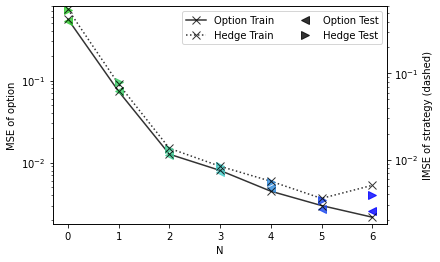
(a) Learning performance

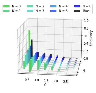
(b) Payoff distribution on test set

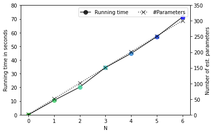
(c) Running time and number of parameters

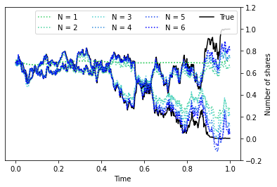
(d) $\theta$ and $\theta^{(N)}$ for two samples of test set

Figure 1. Learning the European call option $G$ in (18) by $G^{\varphi_{0:N}}$, $N=0,...,6$. The learning performance is displayed in (a) in terms of the mean squared error (MSE) $\sum_{m=1}^{M}\left|G(\omega_{m})-G^{\varphi_{0:N}}(\omega_{m})\right|^{2}$ and the integrated mean squared error (IMSE) $\sum_{m=1}^{M}\sum_{k=0}^{K}\left|\theta_{t_{k}}(\omega_{m})-\theta^{(N)}_{t_{k}}(\omega_{m})\right|^{2}$, where the hedging strategy $\theta$ of $G$ is defined in (19) and the approximating hedging strategies $\theta^{(N)}$ of $G^{\varphi_{0:N}}$ are computed with (17). In (c), the running time^3.2 on an average laptop¹ and the number of parameters in the linear regression are depicted. The distributions of $G$ and $G^{\varphi_{0:N}}$ are compared in (b) on the test set, whereas $\theta$ and $\theta^{(N)}$ of two samples in the test set are shown in (d).

3.2. Asian Option in Local Volatility Model

In the second example (see Figure 2), we consider an Asian option in the CEV model (see [Cox, 1975]), where the price process $X=(X_{t})_{t\in[0,T]}$ with $T=1$ follows

$$dX_{t}=\alpha X_{t}dt+\sigma_{0}\sqrt{X_{t}}dB_{t},$$

for $t\in[0,T]$, with $X_{0}=100$, $\alpha=-0.02$, and $\sigma_{0}=0.4$. Hereby, $X$ is a diffusion process with drift $b(t,x)=\alpha x$ and diffusion coefficient $a(t,x)=\sigma_{0}^{2}x$ of linear growth. Then, we learn the Asian option

$$G=\max\left(K-\frac{1}{T}\int_{0}^{T}X_{t}dt,0\right),$$ (20)

with strike price $K=102$. By using similar Fourier arguments as in [Carr and Madan, 1999], we have

$$\mathbb{E}^{\mathbb{Q}}[G|\mathcal{F}_{t}]=\left(K-I_{0,t}\right)\underbrace{\mathbb{E}^{\mathbb{Q}}\left[\mathds{1}_{\left\{I_{t,T}\leq K\right\}}\Big{|}\mathcal{F}_{t}\right]}_{=\frac{1}{2}+\frac{1}{\pi}\int_{0}^{\infty}\operatorname{Re}\left(\frac{e^{-iKu}\varphi_{t}(0,u)}{iu}\right)du}-\underbrace{\mathbb{E}^{\mathbb{Q}}\left[I_{t,T}\mathds{1}_{\left\{I_{t,T}\leq K\right\}}\Big{|}\mathcal{F}_{t}\right]}_{=\frac{T-t}{2T}X_{t}+\frac{1}{\pi}\int_{0}^{\infty}\operatorname{Re}\left(\frac{e^{-iKu}\frac{\partial\varphi_{t}}{\partial z_{2}}(0,u)}{iu}\right)du},$$ (21)

where $I_{r,s}:=\frac{1}{T}\int_{r}^{s}X_{t}dt$ and $\varphi_{t}:\mathbb{C}\times\mathbb{C}\rightarrow\mathbb{C}$ denotes the characteristic function of $\left(X_{T},I_{t,T}\right)|X_{t}$ under the unique ELMM $\mathbb{Q}\sim\mathbb{P}$. Hence, the true hedging strategy $\theta$ is obtained by taking the derivative in (21) with respect to $X_{t}$ and applying the fractional fast Fourier transform (FFT) in [Chourdakis, 2005] to compute the integrals. Hereby, the characteristic function is calculated with the affine transform formula in [Duffie et al., 2000, Section 2.2] and the time-integral extension in [Keller-Ressel, 2009, Section 4.3].

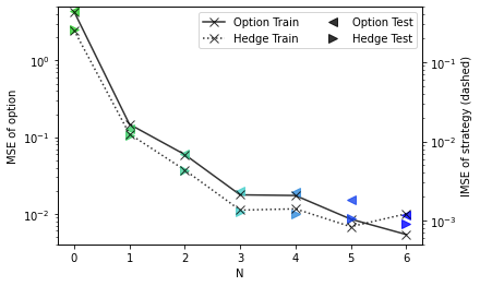
(a) Learning performance

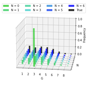
(b) Payoff distribution on test set

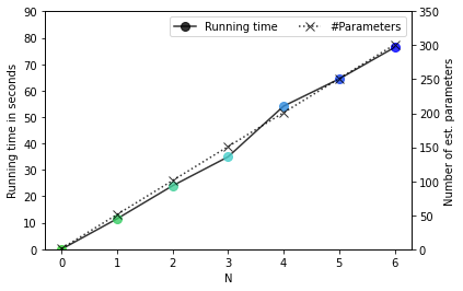
(c) Running time and number of parameters

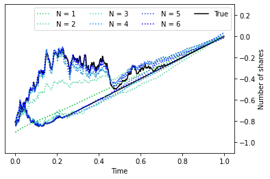
(d) $\theta$ and $\theta^{(N)}$ for two samples of test set

Figure 2. Learning the Asian put option $G$ in (20) by $G^{\varphi_{0:N}}$, $N=0,...,6$. The learning performance is displayed in (a) in terms of the mean squared error (MSE) $\sum_{m=1}^{M}\left|G(\omega_{m})-G^{\varphi_{0:N}}(\omega_{m})\right|^{2}$ and the integrated mean squared error (IMSE) $\sum_{m=1}^{M}\sum_{k=0}^{K}\left|\theta_{t_{k}}(\omega_{m})-\theta^{(N)}_{t_{k}}(\omega_{m})\right|^{2}$, where the hedging strategy $\theta$ of $G$ is computed with the help of (21) and the approximating hedging strategies $\theta^{(N)}$ of $G^{\varphi_{0:N}}$ are calculated with (17). In (c), the running time^3.2 on an average laptop¹ and the number of parameters in the linear regression are depicted. The distributions of $G$ and $G^{\varphi_{0:N}}$ are compared in (b) on the test set, whereas $\theta$ and $\theta^{(N)}$ of two samples in the test set are shown in (d).

3.3. Basket Option in Affine Model

In the third example (see Figure 3), we learn a Basket option written on $d=10$ stocks with $l=10$ Brownian motions. More precisely, we consider for $T=1$ the affine SDE

$$dX_{t}=b(X_{t})dt+\sqrt{a(X_{t})}dB_{t},\quad t\in[0,T],\quad b(x)=\beta_{0}+\sum_{k=1}^{d}\beta_{k}x_{k},\quad a(x)=\alpha_{0}+\sum_{k=1}^{d}\alpha_{k}x_{k}$$

for $X_{0}=(10,...,10)^{\top}$, where $\beta_{k}=(\beta_{k,1},...,\beta_{k,d})^{\top}\in\mathbb{R}^{d}$ and $\alpha_{k}=r_{k}r_{k}^{\top}\in\mathbb{S}^{d}_{+}$, $k=0,...,d$, for some $r_{k}=(r_{k,1},...,r_{k,d})^{\top}\in\mathbb{R}^{d}$, $k=1,...,d$. The parameters are sampled according to $\beta_{0,i}\sim\mathcal{N}(0,3\cdot 10^{-3})$, $\beta_{k,i}\sim\mathcal{N}(0,3\cdot 10^{-4})$, $r_{0,i}\sim\mathcal{N}(0,3\cdot 10^{-2})$, and $r_{k,i}\sim\mathcal{N}(0,3\cdot 10^{-3})$, for all $k,i=1,...,d$. In this case, $X$ is a diffusion process with drift and diffusion coefficient of linear growth. Then, we learn the Basket option

$$G=\max\left(K-w^{\top}X_{T},0\right),$$ (22)

with strike price $K=4$ and $w=(1,-0.95,0.9,-0.85,...,0.6,-0.55)^{\top}\in\mathbb{R}^{d}$. By using similar Fourier arguments as in [Carr and Madan, 1999], we conclude that

$$\mathbb{E}^{\mathbb{Q}}[G|\mathcal{F}_{t}]=K\underbrace{\mathbb{E}^{\mathbb{Q}}\left[\mathds{1}_{\left\{w^{\top}X_{T}\leq K\right\}}\Big{|}\mathcal{F}_{t}\right]}_{=\frac{1}{2}+\frac{1}{\pi}\int_{0}^{\infty}\operatorname{Re}\left(\frac{\exp\left(-iKu\right)\varphi_{t}(uw)}{iu}\right)du}-\underbrace{\mathbb{E}^{\mathbb{Q}}\left[w^{\top}X_{T}\mathds{1}_{\left\{w^{\top}X_{T}\leq K\right\}}\Big{|}\mathcal{F}_{t}\right]}_{=\frac{1}{2}w^{\top}X_{t}+\frac{1}{\pi}\int_{0}^{\infty}\operatorname{Re}\left(\frac{\exp\left(-iKu\right)\psi_{t}(uw)}{iu}\right)du},$$ (23)

where $\varphi_{t}(u)=\mathbb{E}^{\mathbb{Q}}\left[\exp\left(iv^{\top}X_{T}\right)\big{|}\mathcal{F}_{t}\right]$ and $\psi_{t}(v)=\mathbb{E}^{\mathbb{Q}}\left[w^{\top}X_{T}\exp\left(iv^{\top}X_{T}\right)\big{|}\mathcal{F}_{t}\right]$, for $v\in\mathbb{R}^{d}$ and $\mathbb{Q}$ an ELMM. Hence, the true hedging strategy $\theta=\left(\theta^{1}_{t},...,\theta^{10}_{t}\right)_{t\in[0,T]}^{\top}$ is given as the gradient of (23) with respect to $X_{t}$, where the integrals are computed as in Section 3.2. Now, the sample size and the size of the random neural networks are increased to $M=5\cdot 10^{5}$ and $m_{n}=250$, respectively.

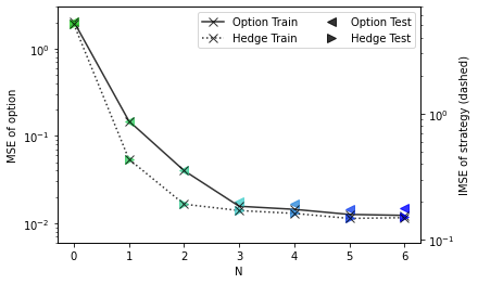
(a) Learning performance

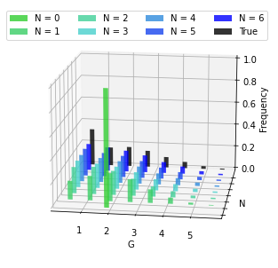
(b) Payoff distribution on test set

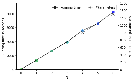
(c) Running time and number of parameters

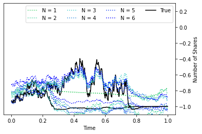
(d1) $\theta^{1}$ and $\theta^{(N),1}$ for two samples of test set

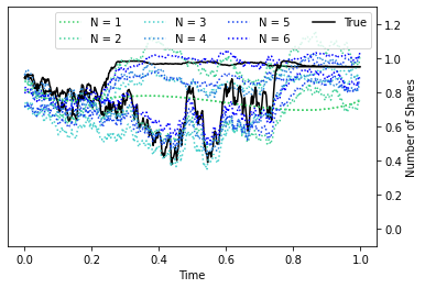
(d2) $\theta^{2}$ and $\theta^{(N),2}$ for two samples of test set

Figure 3. Learning the Basket option $G$ in (22) by $G^{\varphi_{0:N}}$, $N=0,...,6$. The learning performance is displayed in (a) in terms of the mean squared error (MSE) $\sum_{m=1}^{M}\left|G(\omega_{m})-G^{\varphi_{0:N}}(\omega_{m})\right|^{2}$ and the integrated mean squared error (IMSE) $\sum_{m=1}^{M}\sum_{k=0}^{K}\left\|\theta_{t_{k}}(\omega_{m})-\theta^{(N)}_{t_{k}}(\omega_{m})\right\|^{2}$, where the hedging strategy $\theta=\left(\theta^{1}_{t},...,\theta^{10}_{t}\right)_{t\in[0,T]}^{\top}$ of $G$ is computed with the help of (23) and the approximating hedging strategies $\theta^{(N)}=\left(\theta^{(N),1}_{t},...,\theta^{(N),10}_{t}\right)_{t\in[0,T]}^{\top}$ of $G^{\varphi_{0:N}}$ are calculated with (17). In (c), the running time^3.2 on an average laptop¹ and the number of parameters in the linear regression are depicted. The distributions of $G$ and $G^{\varphi_{0:N}}$ are compared in (b) on the test set, whereas $\theta$ and $\theta^{(N)}$ of two samples in the test set are shown in (d1)-(d10).

(d3) $\theta^{3}$ and $\theta^{(N),3}$ for two samples of test set

(d4) $\theta^{4}$ and $\theta^{(N),4}$ for two samples of test set

(d5) $\theta^{5}$ and $\theta^{(N),5}$ for two samples of test set

(d6) $\theta^{6}$ and $\theta^{(N),6}$ for two samples of test set

(d7) $\theta^{7}$ and $\theta^{(N),7}$ for two samples of test set

(d8) $\theta^{8}$ and $\theta^{(N),8}$ for two samples of test set

(d9) $\theta^{9}$ and $\theta^{(N),9}$ for two samples of test set

(d10) $\theta^{10}$ and $\theta^{(N),10}$ for two samples of test set

4. Proofs

In this chapter, we provide all the proofs of the previous results in chronological order.

4.1. Proof of Results in Section 2.1: Stochastic Integral and Quadratic Variation

Proof of Lemma 2.4.

For every $k\in\mathbb{N}$, we define the stopping time $\tau_{k}:=\inf\left\{t\geq 0:\|X_{t}\|\geq k\right\}\wedge T$. Moreover, we fix some $k\in\mathbb{N}$ and $n\in\mathbb{N}\cap[2,\infty)$ in the following. By applying Ito’s formula with respect to the smooth function $\mathbb{R}^{d}\ni x\mapsto f(x):=\|x\|^{2n}\in\mathbb{R}$, it follows for every $t\in[0,T]$, $\mathbb{P}$-a.s., that

$$\|X_{t\wedge\tau_{k}}\|^{2n} =\|X_{0}\|^{2n}+2n\int_{0}^{t}\mathds{1}_{\{s\leq\tau_{k}\}}\|X_{s}\|^{2n-2}X_{s}^{\top}b(s,X_{s})ds$$ (24)

$$\quad\quad...+2n\underbrace{\int_{0}^{t}\mathds{1}_{\{s\leq\tau_{k}\}}\|X_{s}\|^{2n-2}X_{s}^{\top}\sigma(s,X_{s})dB_{s}}_{=:M^{(k)}_{t}}$$

$$\quad\quad...+n\int_{0}^{t}\mathds{1}_{\{s\leq\tau_{k}\}}\|X_{s}\|^{2n-4}\operatorname*{tr}\left(\left((2n-2)X_{s}X_{s}^{\top}-\|X_{s}\|^{2}I_{d}\right)a(s,X_{s})\right)ds.$$

Hereby, we observe by applying the Burkholder-Davis-Gundy inequality (with constant $C_{2}>0$) and using the linear growth condition of $a$ that

$$\mathbb{E}\left[\sup_{t\in[0,T]}\left|M^{(k)}_{t}\right|^{2}\right] \leq C_{2}\mathbb{E}\left[\int_{0}^{T}\mathds{1}_{\{s\leq\tau_{k}\}}\|X_{s}\|^{4n-4}X_{s}^{\top}a(s,X_{s})X_{s}ds\right]$$

$$\leq C_{2}\int_{0}^{T}\mathbb{E}\left[\mathds{1}_{\{s\leq\tau_{k}\}}\|X_{s}\|^{4n-2}\|a(s,X_{s})\|_{F}\right]ds$$

$$\leq C_{2}C_{L}\int_{0}^{T}\mathbb{E}\left[\|X_{s\wedge\tau_{k}}\|^{4n-2}\left(1+\|X_{s\wedge\tau_{k}}\|\right)\right]ds$$

$$\leq C_{2}C_{L}Tk^{4n-2}(1+k)<\infty,$$

which shows that $M^{(k)}$ is a martingale with $\mathbb{E}\left[M^{(k)}_{t}\right]=0$, for all $t\in[0,T]$. Hence, by taking the expectation in (24), and using the Cauchy-Schwarz inequality, Fubini’s theorem, the linear growth condition of $a$ and $b$, the inequalities $\operatorname*{tr}\left(A^{\top}B\right)\leq\|A\|_{F}\|B\|_{F}$, $\|A+B\|_{F}\leq\|A\|_{F}+\|B\|_{F}$ for any $A,B\in\mathbb{R}^{d\times d}$, $\left\|xx^{\top}\right\|_{F}=\sqrt{\operatorname*{tr}\left(xx^{\top}xx^{\top}\right)}=\|x\|^{2}$ for any $x\in\mathbb{R}^{d}$, $\|I_{d}\|_{F}=\sqrt{d}$, and Jensen’s inequality, it follows for every $t\in[0,T]$ that

$$\mathbb{E}\left[\left\|X_{t\wedge\tau_{k}}\right\|^{2n}\right]=\|X_{0}\|^{2n}+{2n}\mathbb{E}\left[\int_{0}^{t}\mathds{1}_{\{s\leq\tau_{k}\}}\|X_{s}\|^{2n-2}X_{s}^{\top}b(s,X_{s})ds\right]$$ (25)

$$\quad\quad\quad\quad...+n\int_{0}^{t}\mathbb{E}\left[\mathds{1}_{\{s\leq\tau_{k}\}}\|X_{s}\|^{2n-4}\operatorname*{tr}\left(\left((2n-2)X_{s}X_{s}^{\top}-\|X_{s}\|^{2}I_{d}\right)a(s,X_{s})\right)\right]ds$$

$$\quad\quad\leq\|X_{0}\|^{2n}+2n\int_{0}^{t}\mathbb{E}\left[\mathds{1}_{\{s\leq\tau_{k}\}}\|X_{s}\|^{2n-1}\|b(s,X_{s})\|\right]ds$$

$$\quad\quad\quad\quad...+n\int_{0}^{t}\mathbb{E}\left[\mathds{1}_{\{s\leq\tau_{k}\}}\left\|X_{s}\right\|^{2n-4}\left\|(2n-2)X_{s}X_{s}^{\top}-\|X_{s}\|^{2}I_{d}\right\|_{F}\|a(s,X_{s})\|_{F}\right]ds$$

$$\quad\quad\leq\|X_{0}\|^{2n}+2nC_{L}\sqrt{d}\int_{0}^{t}\mathbb{E}\left[\|X_{s\wedge\tau_{k}}\|^{2n-1}\left(1+\|X_{s\wedge\tau_{k}}\|\right)\right]ds$$

$$\quad\quad\quad\quad...+nC_{L}\underbrace{\left(2n-2+\sqrt{d}\right)}_{\leq 4n\sqrt{d}}\int_{0}^{t}\mathbb{E}\left[\left\|X_{s\wedge\tau_{k}}\right\|^{2n-2}\left(1+\|X_{s\wedge\tau_{k}}\|\right)\right]ds$$

$$\quad\quad\leq\underbrace{\max\left(\|X_{0}\|,2n\right)^{2n}}_{=:u_{0}}+\int_{0}^{t}\xi_{X}\left(\mathbb{E}\left[\left\|X_{s\wedge\tau_{k}}\right\|^{2n}\right]\right)ds,$$

where $[0,\infty)\ni y\mapsto\xi_{X}(y):=2nC_{L}\sqrt{d}\left(y+y^{\frac{2n-1}{2n}}\right)+4n^{2}C_{L}\sqrt{d}\left(y^{\frac{2n-1}{2n}}+y^{\frac{2n-2}{2n}}\right)\in[0,\infty)$ is continuous with $\xi_{X}(y)>0$, for all $y\in(0,\infty)$. From this, we define $[u_{0},\infty)\ni u\mapsto\Xi_{X}(u):=\int_{u_{0}}^{u}\frac{1}{\xi_{X}(y)}dy\in[0,\infty)$ with $\Xi_{X}^{\prime}(u)=\frac{1}{\xi_{X}(u)}>0$, for all $u\in(u_{0},\infty)$. By the inverse function theorem, there exists a continuously differentiable inverse $\Xi_{X}^{-1}:(0,\infty)\rightarrow(u_{0},\infty)$, with $\left(\Xi_{X}^{-1}\right)^{\prime}(v)=\frac{1}{\xi_{X}\left(\Xi_{X}^{-1}(v)\right)}>0$, for all $v\in(0,\infty)$, implying that $\Xi_{X}^{-1}:(0,\infty)\rightarrow(u_{0},\infty)$ is strictly increasing. Moreover, since $y\geq y^{\frac{2n-1}{2n}}\geq y^{\frac{2n-2}{2n}}$ for all $y\geq u_{0}$, as $u_{0}\geq 1$, and $y\geq 2ny^{\frac{2n-1}{2n}}$ for all $y\geq u_{0}$, as $u_{0}\geq 4n^{2}$, we observe for every $u\in(u_{0},\infty)$ that

$$\Xi_{X}(u) =\int_{u_{0}}^{u}\frac{1}{2nC_{L}\sqrt{d}\left(y+y^{\frac{2n-1}{2n}}\right)+4n^{2}C_{L}\sqrt{d}\left(y^{\frac{2n-1}{2n}}+y^{\frac{2n-2}{2n}}\right)}dy$$

$$\geq\int_{u_{0}}^{u}\frac{1}{4nC_{L}\sqrt{d}\left(y+2ny^{\frac{2n-1}{2n}}\right)}dy\geq\int_{u_{0}}^{u}\frac{1}{8nC_{L}\sqrt{d}y}dy$$

$$=\frac{1}{8nC_{L}\sqrt{d}}\log\left(\frac{u}{u_{0}}\right)=\frac{\log(u)}{8nC_{L}\sqrt{d}}-\frac{\log\left(\max\left(\|X_{0}\|,2n\right)\right)}{4C_{L}\sqrt{d}}>0,$$

which shows that $\Xi_{X}^{-1}(v)\leq\max\left(\|X_{0}\|,2n\right)^{2n}\exp\left(8nC_{L}\sqrt{d}v\right)$, for all $v\in(0,\infty)$. Then, by using (25) together with the non-linear Gronwall inequality in [Bihari, 1956, Equation 6-8] and that $\Xi_{X}(u_{0})=0$, it follows for every $t\in[0,T]$, $k\in\mathbb{N}$, and $n\in\mathbb{N}\cap[2,\infty)$ that

$$\mathbb{E}\left[\left\|X_{t\wedge\tau_{k}}\right\|^{2n}\right]\leq\Xi_{X}^{-1}\left(\Xi_{X}(u_{0})+t\right)\leq\Xi_{X}^{-1}(T)\leq\max\left(\|X_{0}\|,2n\right)^{2n}e^{8nC_{L}\sqrt{d}T},$$

where the right hand-side does not depend on $k\in\mathbb{N}$. Since $\left\|X_{t\wedge\tau_{k}}\right\|^{2n}$ converges $\mathbb{P}$-a.s. to $\|X_{t}\|^{2n}$, as $k\rightarrow\infty$, Fatou’s lemma implies for every $t\in[0,T]$ and $n\in\mathbb{N}\cap[2,\infty)$ that

$$\mathbb{E}\left[\|X_{t}\|^{2n}\right]\leq\liminf_{k\rightarrow\infty}\mathbb{E}\left[\left\|X_{t\wedge\tau_{k}}\right\|^{2n}\right]\leq\max\left(\|X_{0}\|,2n\right)^{2n}e^{8nC_{L}\sqrt{d}T}<\infty,$$

which shows the inequality in (4).

In order to show (5), fix some $0\leq\varepsilon<\exp\left(-4C_{L}\sqrt{d}T-1\right)$. Then, by using (4), Stirling’s inequality, i.e. $r!\geq\sqrt{2\pi r}e^{-r}r^{r}$ for any $r\in\mathbb{N}$, and that $\lim_{n\rightarrow\infty}(4\pi n)^{1/n}=1$, it follows that

$$\limsup_{n\rightarrow\infty}\sqrt[n]{\frac{\varepsilon^{2n}\mathbb{E}\left[\|X_{t}\|^{2n}\right]}{(2n)!}}\leq\limsup_{n\rightarrow\infty}\frac{\varepsilon^{2}\max\left(\|X_{0}\|,2n\right)^{2}e^{8C_{L}\sqrt{d}T}}{(4\pi n)^{\frac{1}{n}}e^{-2}(2n)^{2}}=\left(\varepsilon e^{4C_{L}\sqrt{d}T+1}\right)^{2}<1.$$

Hence, by the root test, $\sum_{n=2}^{\infty}\frac{\varepsilon^{2n}\mathbb{E}\left[\|X_{t}\|^{2n}\right]}{(2n)!}$ converges absolutely. Similarly, by using (4), Stirling’s inequality, i.e. $r!\geq\sqrt{2\pi r}e^{-r}r^{r}$ for any $r\in\mathbb{N}$, and that $\lim_{n\rightarrow\infty}(2\pi(2n-1))^{1/n}=1$, it follows that

$$\limsup_{n\rightarrow\infty}\sqrt[n]{\frac{\varepsilon^{2n-1}\mathbb{E}\left[\|X_{t}\|^{2n}\right]^{\frac{2n-1}{2n}}}{(2n-1)!}} \leq\limsup_{n\rightarrow\infty}\frac{\varepsilon^{\frac{2n-1}{n}}\max\left(\|X_{0}\|,2n\right)^{\frac{2n-1}{n}}e^{4\frac{2n-1}{n}C_{L}\sqrt{d}T}}{(2\pi(2n-1))^{\frac{1}{n}}e^{-\frac{2n-1}{n}}(2n-1)^{\frac{2n-1}{n}}}$$

$$=\limsup_{n\rightarrow\infty}\left(\varepsilon e^{4C_{L}\sqrt{d}T+1}\right)^{\frac{2n-1}{n}}=\left(\varepsilon e^{4C_{L}\sqrt{d}T+1}\right)^{2}<1.$$

Hence, by the root test, $\sum_{n=3}^{\infty}\frac{\varepsilon^{2n-1}\mathbb{E}\left[\|X_{t}\|^{2n}\right]^{(2n-1)/(2n)}}{(2n-1)!}$ converges absolutely. Finally, by using the monotone convergence theorem, Jensen’s inequality, and (4) with $n=2$ implying that $\sum_{n=1}^{3}\frac{\varepsilon^{n}\mathbb{E}\left[\|X_{t}\|^{4}\right]^{\frac{n}{4}}}{n!}<\infty$, it follows for every $t\in[0,T]$ that

$$\mathbb{E}\left[e^{\varepsilon\|X_{t}\|}\right] =\sum_{n=0}^{\infty}\frac{\varepsilon^{n}\mathbb{E}\left[\|X_{t}\|^{n}\right]}{n!}$$

$$=1+\sum_{n=1}^{3}\frac{\varepsilon^{n}\mathbb{E}\left[\|X_{t}\|^{n}\right]}{n!}+\sum_{n=2}^{\infty}\frac{\varepsilon^{2n}\mathbb{E}\left[\|X_{t}\|^{2n}\right]}{(2n)!}+\sum_{n=3}^{\infty}\frac{\varepsilon^{2n-1}\mathbb{E}\left[\|X_{t}\|^{2n-1}\right]}{(2n-1)!}$$

$$\leq 1+\sum_{n=1}^{3}\frac{\varepsilon^{n}\mathbb{E}\left[\|X_{t}\|^{4}\right]^{\frac{n}{4}}}{n!}+\sum_{n=2}^{\infty}\frac{\varepsilon^{2n}\mathbb{E}\left[\|X_{t}\|^{2n}\right]}{(2n)!}+\sum_{n=3}^{\infty}\frac{\varepsilon^{2n-1}\mathbb{E}\left[\|X_{t}\|^{2n}\right]^{\frac{2n-1}{2n}}}{(2n-1)!}<\infty,$$

which completes the proof. ∎

Proof of Lemma 2.5.

First, we use the linear growth of $a$ and $b$, the inequalities $(x+y)^{r}\leq 2^{r-1}\left(x^{r}+y^{r}\right)$ and $(x+y)^{1/r}\leq x^{1/r}+y^{1/r}$ for any $x,y\geq 0$ and $r\in[1,\infty)$, and Lemma 2.4 to conclude that

$$C_{p,T,X} :=T^{\max\left(\frac{1}{2},\frac{p-1}{p}\right)}\sup_{t\in[0,T]}\mathbb{E}\left[\|b(t,X_{t})\|^{\max(2,p)}\right]^{\frac{1}{\max(2,p)}}$$ (26)

$$\quad\quad...+T^{\max\left(0,\frac{p-2}{2p}\right)}\sup_{t\in[0,T]}\mathbb{E}\left[\|a(t,X_{t})\|_{F}^{\max\left(1,\frac{p}{2}\right)}\right]^{\frac{1}{\max(2,p)}}$$

$$\leq C_{L}T^{\max\left(\frac{1}{2},\frac{p-1}{p}\right)}\sup_{t\in[0,T]}\mathbb{E}\left[\left(1+\|X_{t}\|\right)^{\max(2,p)}\right]^{\frac{1}{\max(2,p)}}$$

$$\quad\quad...+\sqrt{C_{L}}T^{\max\left(0,\frac{p-2}{2p}\right)}\sup_{t\in[0,T]}\mathbb{E}\left[\left(1+\|X_{t}\|\right)^{\max\left(1,\frac{p}{2}\right)}\right]^{\frac{1}{\max(2,p)}}$$

$$\leq\left(2^{\max(2,p)-1}\right)^{\frac{1}{\max(2,p)}}C_{L}T^{\max\left(\frac{1}{2},\frac{p-1}{p}\right)}\left(1+\sup_{t\in[0,T]}\mathbb{E}\left[\|X_{t}\|^{\max(2,p)}\right]^{\frac{1}{\max(2,p)}}\right)$$

$$\quad\quad...+\left(2^{\max(1,p/2)-1}\right)^{\frac{1}{\max(2,p)}}\sqrt{C_{L}}T^{\max\left(0,\frac{p-2}{2p}\right)}\left(1+\sup_{t\in[0,T]}\mathbb{E}\left[\|X_{t}\|^{\max\left(1,\frac{p}{2}\right)}\right]^{\frac{1}{\max(2,p)}}\right)$$

$$\leq 2C_{L}T^{\max\left(\frac{1}{2},\frac{p-1}{p}\right)}\left(1+\sup_{t\in[0,T]}\mathbb{E}\left[\|X_{t}\|^{\max(2,p)}\right]^{\frac{1}{\max(2,p)}}\right)$$

$$\quad\quad...+\sqrt{2C_{L}}T^{\max\left(0,\frac{p-2}{2p}\right)}\left(1+\sup_{t\in[0,T]}\mathbb{E}\left[\|X_{t}\|^{\max\left(1,\frac{p}{2}\right)}\right]^{\frac{1}{\max(2,p)}}\right)<\infty.$$

Now, we fix some $g\in D_{l}([0,T];\mathbb{R}^{d})$. By [Fraňková, 1991, Lemma 1.5], $g:[0,T]\rightarrow\mathbb{R}^{d}$ is a uniform limit of $\mathbb{R}^{d}$-valued piecewise constant functions. Since the latter are $\mathcal{B}([0,T])/\mathcal{B}(\mathbb{R}^{d})$-measurable, we conclude that $g:[0,T]\rightarrow\mathbb{R}^{d}$ is also $\mathcal{B}([0,T])/\mathcal{B}(\mathbb{R}^{d})$-measurable. Moreover, by using [Fraňková, 1991, Lemma 1.7], it follows that $g:[0,T]\rightarrow\mathbb{R}^{d}$ is bounded, which implies that $\|g\|_{\infty}:=\sup_{t\in[0,T]}\|g(t)\|<\infty$. Hence, by using Jensen’s inequality for the time integral of a convex function, Jensen’s inequality for the expectation of a concave function (if $p/2\in[1/2,1]$) or Jensen’s inequality for the time integral of a convex function (if $p/2\in(1,\infty)$), Fubini’s theorem, and (26), we conclude that

$$\|g\|_{L^{p}(X)} =\mathbb{E}\left[\left(\int_{0}^{T}\left|g(t)^{\top}b(t,X_{t})\right|dt\right)^{p}\right]^{\frac{1}{p}}+\mathbb{E}\left[\left(\int_{0}^{T}g(t)^{\top}a(t,X_{t})g(t)dt\right)^{\frac{p}{2}}\right]^{\frac{1}{p}}$$

$$\leq\sqrt{T}\mathbb{E}\left[\left(\int_{0}^{T}\|g(t)\|^{2}\|b(t,X_{t})\|^{2}dt\right)^{\frac{p}{2}}\right]^{\frac{1}{p}}+\mathbb{E}\left[\left(\int_{0}^{T}\|g(t)\|^{2}\|a(t,X_{t})\|_{F}dt\right)^{\frac{p}{2}}\right]^{\frac{1}{p}}$$

$$\leq\sqrt{T}T^{\max\left(0,\frac{1}{2}-\frac{1}{p}\right)}\left(\int_{0}^{T}\mathbb{E}\left[\|g(t)\|^{\max(2,p)}\|b(t,X_{t})\|^{\max(2,p)}\right]dt\right)^{\frac{1}{\max(2,p)}}$$

$$\quad\quad...+T^{\max\left(0,\frac{1}{2}-\frac{1}{p}\right)}\left(\int_{0}^{T}\mathbb{E}\left[\|g(t)\|^{\max(2,p)}\|a(t,X_{t})\|_{F}^{\max\left(1,\frac{p}{2}\right)}\right]dt\right)^{\frac{1}{{\max(2,p)}}}$$

$$\leq T^{\max\left(\frac{1}{2},\frac{p-1}{p}\right)}\sup_{t\in[0,T]}\mathbb{E}\left[\|b(t,X_{t})\|^{\max(2,p)}\right]^{\frac{1}{\max(2,p)}}\left(\int_{0}^{T}\|g(t)\|^{\max(2,p)}dt\right)^{\frac{1}{\max(2,p)}}$$

$$\quad\quad...+T^{\max\left(0,\frac{p-2}{2p}\right)}\sup_{t\in[0,T]}\mathbb{E}\left[\|a(t,X_{t})\|_{F}^{\max\left(1,\frac{p}{2}\right)}\right]^{\frac{1}{\max(2,p)}}\left(\int_{0}^{T}\|g(t)\|^{\max(2,p)}dt\right)^{\frac{1}{\max(2,p)}}$$

$$\leq C_{p,T,X}\|g\|_{L^{\max(2,p)}([0,T],\mathcal{B}([0,T]),dt;\mathbb{R}^{d})}\leq C_{p,T,X}T^{\frac{1}{\max(2,p)}}\|g\|_{\infty}<\infty,$$

which completes the proof. ∎

Proof of Lemma 2.8.

For two functions $f,g\in D_{l}([0,T];\mathbb{R}^{d})$ and some $\lambda\in\mathbb{R}$, it follows that $f+g\in D_{l}([0,T];\mathbb{R}^{d})$ and $\lambda\cdot f\in D_{l}([0,T];\mathbb{R}^{d})$. Hence, we only need to show that $\|\cdot\|_{L^{p}(X)}$ is a norm. By definition, $\|\cdot\|_{L^{p}(X)}$ is absolutely homogeneous, and since we consider $L^{p}(X)$ as quotient space with respect to the kernel of $\|\cdot\|_{L^{p}(X)}$, the norm $\|\cdot\|_{L^{p}(X)}$ is positive definite. In order to show the triangle inequality, let $f,g\in L^{p}(X)$. Then, by applying the Cauchy-Schwarz inequality twice, it holds $\mathbb{P}$-a.s. that

$$\int_{0}^{T}f(t)^{\top}a(t,X_{t})g(t)dt=\int_{0}^{T}f(t)^{\top}\sigma(t,X_{t})\sigma(t,X_{t})^{\top}g(t)dt$$

$$\quad\quad\leq\int_{0}^{T}\left(f(t)^{\top}\sigma(t,X_{t})\sigma(t,X_{t})^{\top}f(t)\right)^{\frac{1}{2}}\left(g(t)^{\top}\sigma(t,X_{t})\sigma(t,X_{t})^{\top}g(t)\right)^{\frac{1}{2}}dt$$

$$\quad\quad\leq\left(\int_{0}^{T}f(t)^{\top}a(t,X_{t})f(t)dt\right)^{\frac{1}{2}}\left(\int_{0}^{T}g(t)^{\top}a(t,X_{t})g(t)dt\right)^{\frac{1}{2}}=Q(f)^{\frac{1}{2}}Q(g)^{\frac{1}{2}},$$

Hence, by using $x+2\sqrt{xy}+y=(\sqrt{x}+\sqrt{y})^{2}$ for any $x,y\geq 0$, it follows that

$$Q(f+g) =Q(f)+2\int_{0}^{T}f(t)^{\top}a(t,X_{t})g(t)dt+Q(g)$$

$$\leq Q(f)+2Q(f)^{\frac{1}{2}}Q(g)^{\frac{1}{2}}+Q(g)$$

$$=\left(Q(f)^{\frac{1}{2}}+Q(g)^{\frac{1}{2}}\right)^{2}.$$

Finally, by applying Minkowski’s inequality, we conclude that

$$\|f+g\|_{L^{p}(X)}=\mathbb{E}\left[\left(\int_{0}^{T}\left|(f(t)+g(t))^{\top}b(t,X_{t})\right|dt\right)^{p}\right]^{\frac{1}{p}}+\mathbb{E}\left[Q(f+g)^{\frac{p}{2}}\right]^{\frac{1}{p}}$$

$$\quad\quad\leq\mathbb{E}\left[\left(\int_{0}^{T}\left|f(t)^{\top}b(t,X_{t})\right|dt\right)^{p}\right]^{\frac{1}{p}}+\mathbb{E}\left[\left(\int_{0}^{T}\left|g(t)^{\top}b(t,X_{t})\right|dt\right)^{p}\right]^{\frac{1}{p}}+\mathbb{E}\left[\left(Q(f)^{\frac{1}{2}}+Q(g)^{\frac{1}{2}}\right)^{2}\right]^{\frac{1}{p}}$$

$$\quad\quad\leq\mathbb{E}\left[\left(\int_{0}^{T}\left|f(t)^{\top}b(t,X_{t})\right|dt\right)^{p}\right]^{\frac{1}{p}}+\mathbb{E}\left[\left(\int_{0}^{T}\left|g(t)^{\top}b(t,X_{t})\right|dt\right)^{p}\right]^{\frac{1}{p}}+\mathbb{E}\left[Q(f)^{\frac{p}{2}}\right]^{\frac{1}{p}}+\mathbb{E}\left[Q(g)^{\frac{p}{2}}\right]^{\frac{1}{p}}$$

$$\quad\quad=\|f\|_{L^{p}(X)}+\|g\|_{L^{p}(X)},$$

which completes the proof. ∎

Proof of Lemma 2.11.

In order to prove (7b), let $g\in L^{p}(X)$. Since $t\mapsto Q(g)_{t}$ is non-decreasing and $Q(g)_{T}=Q(g)$ holds by definition of $Q:L^{p}(X)\rightarrow L^{p/2}(\mathbb{P})$, we observe that

$$\mathbb{E}\left[\sup_{t\in[0,T]}Q(g)_{t}^{\frac{p}{2}}\right]^{\frac{1}{p}}=\mathbb{E}\left[Q(g)^{\frac{p}{2}}\right]^{\frac{1}{p}}\leq\|g\|_{L^{p}(X)},$$

which shows (7b). Moreover, by using Minkowski’s inequality and the Burkholder-Davis-Gundy inequality (with constant $C_{p}>0$), it follows that

$$\mathbb{E}\left[\sup_{t\in[0,T]}\left|W(g)_{t}\right|^{p}\right]^{\frac{1}{p}} \leq\mathbb{E}\left[\sup_{t\in[0,T]}\left|\int_{0}^{t}g(s)^{\top}b(s,X_{s})ds\right|^{p}\right]^{\frac{1}{p}}+\mathbb{E}\left[\sup_{t\in[0,T]}\left|\int_{0}^{t}g(s)^{\top}\sigma(s,X_{s})dB_{s}\right|^{p}\right]^{\frac{1}{p}}$$

$$\leq\mathbb{E}\left[\left(\int_{0}^{T}\left|g(s)^{\top}b(s,X_{s})\right|ds\right)^{p}\right]^{\frac{1}{p}}+C_{p}\mathbb{E}\left[\left(\int_{0}^{T}g(s)^{\top}a(s,X_{s})g(s)ds\right)^{\frac{p}{2}}\right]^{\frac{1}{p}}$$

$$\leq\max\left(1,C_{p}\right)\|g\|_{L^{p}(X)},$$

which shows the other inequality in (7a). ∎

Lemma 4.1.

Let $X$ be a diffusion process with coefficients of linear growth with constant $C_{L}>0$, and let $g\in D_{l}([0,T];\mathbb{R}^{d})$. Then, it holds for every $n\in\mathbb{N}\cap[2,\infty)$ that

$$\sup_{t\in[0,T]}\mathbb{E}\left[W(g)_{t}^{2n}\right] \leq n^{2n}\|g\|_{\infty}^{2n}\left(1+16C_{d,L,T,\|X_{0}\|}T\right)^{2n},$$ (27a)

$$\sup_{t\in[0,T]}\mathbb{E}\left[Q(g)_{t}^{n}\right] \leq n^{n}\|g\|_{\infty}^{2n}\left(1+8C_{d,L,T,\|X_{0}\|}T\right)^{n},$$ (27b)

where $C_{d,L,T,\|X_{0}\|}:=C_{L}\max\left(1,\|X_{0}\|\exp\left(4C_{L}\sqrt{d}T\right)\right)>0$ does not depend on $n\in\mathbb{N}$. Moreover, for every $g\in D_{l}([0,T];\mathbb{R}^{d})$ with $\|g\|_{\infty}:=\sup_{t\in[0,T]}\|g(t)\|<2\left(\left(1+16C_{d,L,T,\|X_{0}\|}T\right)e\right)^{-1}$, we have for every $t\in[0,T]$ that

$$\mathbb{E}\left[e^{|W(g)_{t}|}\right]<\infty.$$ (28)

In addition, for every $g\in D_{l}([0,T];\mathbb{R}^{d})$ with $\|g\|_{\infty}^{2}<1/\left(\left(1+4C_{d,L,T,\|X_{0}\|}T\right)e\right)$, we have for every $t\in[0,T]$ that

$$\mathbb{E}\left[e^{Q(g)_{t}}\right]<\infty.$$ (29)

Proof.

In order to show (27a), we first define the sequence of stopping times $\left(\tau^{W}_{k}\right)_{k\in\mathbb{N}}$ by $\tau^{W}_{k}=\inf\left\{t\geq 0:\max\left(|W(g)_{t}|,\|X_{t}\|\right)\geq k\right\}\wedge T$, for $k\in\mathbb{N}$. Now, we fix some $k\in\mathbb{N}$ and $n\in\mathbb{N}\cap[2,\infty)$. Then, by applying Ito’s formula on the smooth function $f(x)=x^{2n}$, it follows for every $t\in[0,T]$, $\mathbb{P}$-a.s., that

$$W(g)_{t\wedge\tau_{k}^{W}}^{2n} =2n\int_{0}^{t}\mathds{1}_{\left\{s\leq\tau_{k}^{W}\right\}}W(g)_{s}^{2n-1}g(s)^{\top}b(s,X_{s})ds$$ (30)

$$\quad\quad...+2n\underbrace{\int_{0}^{t}\mathds{1}_{\left\{s\leq\tau_{k}^{W}\right\}}W(g)_{s}^{2n-1}g(s)^{\top}\sigma(s,X_{s})dB_{s}}_{=:M^{(k)}_{t}}$$

$$\quad\quad...+n(2n-1)\int_{0}^{t}\mathds{1}_{\left\{s\leq\tau_{k}^{W}\right\}}W(g)_{s}^{2n-2}g(s)^{\top}a(s,X_{s})g(s)ds.$$

Hereby, we observe by applying the Burkholder-Davis-Gundy inequality (with constant $C_{2}>0$) and using the linear growth condition of $a$ that

$$\mathbb{E}\left[\sup_{t\in[0,T]}\left|M^{(k)}_{t}\right|^{2}\right] \leq C_{2}\mathbb{E}\left[\int_{0}^{T}\mathds{1}_{\left\{s\leq\tau_{k}^{W}\right\}}W(g)_{s}^{4n-2}g(s)^{\top}a(s,X_{s})g(s)ds\right]$$

$$\leq C_{2}\int_{0}^{T}\mathbb{E}\left[\mathds{1}_{\left\{s\leq\tau_{k}^{W}\right\}}W(g)_{s}^{4n-2}\|g(s)\|^{2}\|a(s,X_{s})\|_{F}\right]ds$$

$$\leq C_{2}C_{L}\|g\|_{\infty}^{2}\int_{0}^{T}\mathbb{E}\left[\left|W(g)_{s\wedge\tau_{k}^{W}}\right|^{4n-2}\left(1+\left\|X_{s\wedge\tau_{k}^{W}}\right\|\right)\right]ds$$

$$\leq C_{2}C_{L}\|g\|_{\infty}^{2}Tk^{4n-2}(1+k)<\infty,$$

which shows that $M^{(k)}$ is a martingale with $\mathbb{E}\left[M^{(k)}_{t}\right]=0$, for all $t\in[0,T]$. Hence, by taking the expectation in (30), using the linear growth condition of $a$ and $b$, Hölder’s inequality (with exponents $\frac{2n-1}{2n}+\frac{1}{2n}=1$ and $\frac{2n-2}{2n}+\frac{2}{2n}=1$, respectively) together with Jensen’s inequality, the inequalities $(x+y)^{2n}\leq 2^{2n-1}\left(x^{2n}+y^{2n}\right)$ and $(x+y)^{n}\leq 2^{n-1}\left(x^{n}+y^{n}\right)$ for any $x,y\geq 0$, Lemma 2.4, the inequalities $(x+y)^{\frac{1}{2n}}\leq x^{\frac{1}{2n}}+y^{\frac{1}{2n}}$ and $(x+y)^{\frac{1}{n}}\leq x^{\frac{1}{n}}+y^{\frac{1}{n}}$ for any $x,y\geq 0$, and defining $C_{d,L,T,\|X_{0}\|}:=C_{L}\max\left(1,\|X_{0}\|\exp\left(4C_{L}\sqrt{d}T\right)\right)>0$, it follows for every $t\in[0,T]$ that

$$\mathbb{E}\left[W(g)_{t\wedge\tau^{W}_{k}}^{2n}\right]=2n\mathbb{E}\left[\int_{0}^{t}\mathds{1}_{\left\{s\leq\tau_{k}^{W}\right\}}W(g)_{s}^{2n-1}g(s)^{\top}b(s,X_{s})ds\right]$$ (31)

$$\quad\quad\quad\quad...+n(2n-1)\mathbb{E}\left[\int_{0}^{t}\mathds{1}_{\left\{s\leq\tau_{k}^{W}\right\}}W(g)_{s}^{2n-2}g(s)^{\top}a(s,X_{s})g(s)ds\right]$$

$$\quad\quad\leq 2n\int_{0}^{t}\mathbb{E}\left[\mathds{1}_{\left\{s\leq\tau_{k}^{W}\right\}}|W(g)_{s}|^{2n-1}\|b(s,X_{s})\|\right]\|g(s)\|ds$$

$$\quad\quad\quad\quad...+n(2n-1)\int_{0}^{t}\mathbb{E}\left[\mathds{1}_{\left\{s\leq\tau_{k}^{W}\right\}}W(g)_{s}^{2n-2}\|a(s,X_{s})\|_{F}\right]\|g(s)\|^{2}ds$$

$$\quad\quad\leq 2n\|g\|_{\infty}C_{L}\int_{0}^{t}\mathbb{E}\left[\mathds{1}_{\left\{s\leq\tau_{k}^{W}\right\}}|W(g)_{s}|^{2n-1}\left(1+\|X_{s}\|\right)\right]ds$$

$$\quad\quad\quad\quad...+n(2n-1)\|g\|_{\infty}^{2}C_{L}\int_{0}^{t}\mathbb{E}\left[\mathds{1}_{\left\{s\leq\tau_{k}^{W}\right\}}W(g)_{s}^{2n-2}\left(1+\|X_{s}\|\right)\right]ds$$

$$\quad\quad\leq\underbrace{\left(2^{2n-1}\right)^{\frac{1}{2n}}}_{\leq 2}2n\|g\|_{\infty}C_{L}\int_{0}^{t}\mathbb{E}\left[W(g)_{s\wedge\tau_{k}^{W}}^{2n}\right]^{\frac{2n-1}{2n}}\mathbb{E}\left[1+\|X_{s}\|^{2n}\right]^{\frac{1}{2n}}ds$$

$$\quad\quad\quad\quad...+\underbrace{\left(2^{2n-1}\right)^{\frac{1}{2n}}}_{\leq 2}n(2n-1)\|g\|_{\infty}^{2}C_{L}\int_{0}^{t}\mathbb{E}\left[W(g)_{s\wedge\tau_{k}^{W}}^{2n}\right]^{\frac{2n-2}{2n}}\mathbb{E}\left[1+\|X_{s}\|^{2n}\right]^{\frac{1}{2n}}ds$$

$$\quad\quad\leq 4n\|g\|_{\infty}C_{L}\left(1+\max\left(\|X_{0}\|,2n\right)^{2n}e^{8nC_{L}\sqrt{d}T}\right)^{\frac{1}{2n}}\int_{0}^{t}\mathbb{E}\left[W(g)_{s\wedge\tau_{k}^{W}}^{2n}\right]^{\frac{2n-1}{2n}}ds$$

$$\quad\quad\quad\quad...+4n^{2}\|g\|_{\infty}^{2}C_{L}\left(1+\max\left(\|X_{0}\|,2n\right)^{2n}e^{8nC_{L}\sqrt{d}T}\right)^{\frac{1}{2n}}\int_{0}^{t}\mathbb{E}\left[W(g)_{s\wedge\tau_{k}^{W}}^{2n}\right]^{\frac{2n-2}{2n}}ds$$

$$\quad\quad\leq 4n\|g\|_{\infty}\underbrace{C_{L}\left(1+\max\left(\|X_{0}\|,2n\right)e^{4C_{L}\sqrt{d}T}\right)}_{\leq 4nC_{d,L,T,\|X_{0}\|}}\int_{0}^{t}\mathbb{E}\left[W(g)_{s\wedge\tau_{k}^{W}}^{2n}\right]^{\frac{2n-1}{2n}}ds$$

$$\quad\quad\quad\quad...+4n^{2}\|g\|_{\infty}^{2}\underbrace{C_{L}\left(1+\max\left(\|X_{0}\|,2n\right)e^{4C_{L}\sqrt{d}T}\right)}_{\leq 4nC_{d,L,T,\|X_{0}\|}}\int_{0}^{t}\mathbb{E}\left[W(g)_{s\wedge\tau_{k}^{W}}^{2n}\right]^{\frac{2n-2}{2n}}ds$$

$$\quad\quad\leq\underbrace{n^{2n}\|g\|_{\infty}^{2n}}_{=:u_{0}}+\int_{0}^{t}\xi_{W}\left(\mathbb{E}\left[W(g)_{s\wedge\tau^{W}_{k}}^{2n}\right]\right)ds,$$

where $[0,\infty)\ni y\mapsto\xi_{W}(y):=16n^{2}C_{d,L,T,\|X_{0}\|}\left(\|g\|_{\infty}y^{\frac{2n-1}{2n}}+n\|g\|_{\infty}^{2}y^{\frac{2n-2}{2n}}\right)\in[0,\infty)$ is continuous with $\xi_{W}(y)>0$, for all $y\in(0,\infty)$. From this, we define $[u_{0},\infty)\ni u\mapsto\Xi_{W}(u):=\int_{u_{0}}^{u}\frac{1}{\xi_{W}(y)}dy\in[0,\infty)$ with $\Xi_{W}^{\prime}(u)=\frac{1}{\xi_{W}(u)}>0$, for all $u\in(u_{0},\infty)$. By the inverse function theorem, there exists a continuously differentiable inverse function $\Xi_{W}^{-1}:(0,\infty)\rightarrow(u_{0},\infty)$ with $\left(\Xi_{W}^{-1}\right)^{\prime}(v)=\frac{1}{\xi_{W}\left(\Xi_{W}^{-1}(v)\right)}>0$, for all $v\in(0,\infty)$, implying that $\Xi_{W}^{-1}:(0,\infty)\rightarrow(u_{0},\infty)$ is strictly increasing. Moreover, since $\|g\|_{\infty}y^{\frac{2n-1}{2n}}\geq n\|g\|_{\infty}^{2}y^{\frac{2n-2}{2n}}$, for all $y\geq u_{0}$, we observe for every $u\in(u_{0},\infty)$ that

$$\Xi_{W}(u) =\int_{u_{0}}^{u}\frac{1}{16n^{2}C_{d,L,T,\|X_{0}\|}\left(\|g\|_{\infty}y^{\frac{2n-1}{2n}}+n\|g\|_{\infty}^{2}y^{\frac{2n-2}{2n}}\right)}dy\geq\int_{u_{0}}^{u}\frac{y^{\frac{1}{2n}-1}}{32n^{2}\|g\|_{\infty}C_{d,L,T,\|X_{0}\|}}dy$$

$$=\frac{u^{\frac{1}{2n}}-u_{0}^{\frac{1}{2n}}}{16n\|g\|_{\infty}C_{d,L,T,\|X_{0}\|}}=\frac{u^{\frac{1}{2n}}}{16n\|g\|_{\infty}C_{d,L,T,\|X_{0}\|}}-\frac{1}{16C_{d,L,T,\|X_{0}\|}}>0,$$

which shows that $\Xi_{W}^{-1}(v)\leq n^{2n}\|g\|_{\infty}^{2n}\left(1+16C_{d,L,T,\|X_{0}\|}v\right)^{2n}$, for all $v\in(0,\infty)$. Then, by using (31) together with the non-linear Gronwall inequality in [Bihari, 1956, Equation 6-8] and that $\Xi_{W}(u_{0})=0$, it follows for every $t\in[0,T]$, $k\in\mathbb{N}$, and $n\in\mathbb{N}\cap[2,\infty)$ that

$$\mathbb{E}\left[W(g)_{t\wedge\tau^{W}_{k}}^{2n}\right]\leq\Xi_{W}^{-1}\left(\Xi_{W}(u_{0})+t\right)\leq\Xi_{W}^{-1}(T)\leq n^{2n}\|g\|_{\infty}^{2n}\left(1+16C_{d,L,T,\|X_{0}\|}T\right)^{2n},$$

where the right-hand side does not depend on $k\in\mathbb{N}$. As $W(g)_{t\wedge\tau^{W}_{k}}^{2n}$ converges $\mathbb{P}$-a.s. to $W(g)_{t}^{2n}$, as $k\rightarrow\infty$, Fatou’s lemma implies for every $t\in[0,T]$ and $n\in\mathbb{N}\cap[2,\infty)$ that

$$\mathbb{E}\left[W(g)_{t}^{2n}\right]\leq\liminf_{k\rightarrow\infty}\mathbb{E}\left[W(g)_{t\wedge\tau^{W}_{k}}^{2n}\right]\leq n^{2n}\|g\|_{\infty}^{2n}\left(1+16C_{d,L,T,\|X_{0}\|}T\right)^{2n},$$

which shows the inequality in (27a).

In order to show (27b), let $n\in\mathbb{N}\cap[2,\infty)$ and define for every $k\in\mathbb{N}$ the stopping time $\tau^{Q}_{k}=\inf\left\{t\geq 0:Q(g)_{t}\geq k\right\}\wedge T$. Then, by Ito’s formula, it follows for every $t\in[0,T]$, $\mathbb{P}$-a.s., that $dQ(g)_{t}^{n}=nQ(g)_{t}^{n-1}dQ(g)_{t}$. Moreover, by using the linear growth condition of $a$, Hölder’s inequality (with exponents $\frac{n-1}{n}+\frac{1}{n}=1$) together with Jensen’s inequality, that $(x+y)^{2n}\leq 2^{2n-1}\left(x^{2n}+y^{2n}\right)$ for any $x,y\geq 0$, Lemma 2.4, and $(x+y)^{\frac{1}{2n}}\leq x^{\frac{1}{2n}}+y^{\frac{1}{2n}}$ for any $x,y\geq 0$, it holds for every $t\in[0,T]$ that

$$\mathbb{E}\left[Q(g)_{t\wedge\tau^{Q}_{k}}^{n}\right] \leq\mathbb{E}\left[\int_{0}^{t}\mathds{1}_{\left\{s\leq\tau^{Q}_{k}\right\}}Q(g)_{s}^{n-1}\|a(s,X_{s})\|_{F}\|g(s)\|^{2}ds\right]$$ (32)

$$\leq nC_{L}\int_{0}^{t}\mathbb{E}\left[\mathds{1}_{\left\{s\leq\tau^{Q}_{k}\right\}}Q(g)_{s}^{n-1}\left(1+\|X_{s}\|\right)\right]\|g(s)\|^{2}ds$$

$$\leq\underbrace{\left(2^{2n-1}\right)^{\frac{1}{2n}}}_{\leq 2}n\|g\|_{\infty}^{2}C_{L}\int_{0}^{t}\mathbb{E}\left[Q(g)_{s\wedge\tau^{Q}_{k}}^{n}\right]^{\frac{n-1}{n}}\mathbb{E}\left[1+\|X_{s}\|^{2n}\right]^{\frac{1}{2n}}ds$$

$$\leq 2n\|g\|_{\infty}^{2}C_{L}\left(1+\max\left(\|X_{0}\|,2n\right)^{2n}e^{8nC_{L}\sqrt{d}T}\right)^{\frac{1}{2n}}\int_{0}^{t}\mathbb{E}\left[Q(g)_{s\wedge\tau^{Q}_{k}}^{n}\right]^{\frac{n-1}{n}}ds$$

$$\leq 2n\|g\|_{\infty}^{2}\underbrace{C_{L}\left(1+\max\left(\|X_{0}\|,2n\right)e^{4C_{L}\sqrt{d}T}\right)}_{\leq 4nC_{d,L,T,\|X_{0}\|}}\int_{0}^{t}\mathbb{E}\left[Q(g)_{s\wedge\tau^{Q}_{k}}^{n}\right]^{\frac{n-1}{n}}ds$$

$$\leq\underbrace{n^{n}\|g\|_{\infty}^{2n}}_{=:u_{0}}+\int_{0}^{t}\xi_{Q}\left(\mathbb{E}\left[Q(g)_{s\wedge\tau^{Q}_{k}}^{n}\right]\right)ds,$$

where $[0,\infty)\ni y\mapsto\xi_{Q}(y):=8n^{2}\|g\|_{\infty}^{2}C_{d,L,T,\|X_{0}\|}y^{\frac{n-1}{n}}\in[0,\infty)$ is continuous with $\xi_{Q}(y)>0$, for all $y\in(0,\infty)$. From this, we define $[u_{0},\infty)\ni u\mapsto\Xi_{Q}(u)=\int_{u_{0}}^{u}\frac{1}{\xi_{Q}(y)}dy\in[0,\infty)$ satisfying $\Xi_{Q}^{\prime}(u)=\frac{1}{\xi_{Q}(u)}>0$, for all $u\in(u_{0},\infty)$. By the inverse function theorem, there exists a continuously differentiable inverse $\Xi_{Q}^{-1}:(0,\infty)\rightarrow(u_{0},\infty)$ with $\left(\Xi_{Q}^{-1}\right)^{\prime}(v)=\frac{1}{\xi_{Q}\left(\Xi_{Q}^{-1}(v)\right)}>0$, for all $v\in(0,\infty)$, implying that $\Xi_{Q}^{-1}:(0,\infty)\rightarrow(u_{0},\infty)$ is strictly increasing. Moreover, for every $u\in(u_{0},\infty)$, we have

$$\Xi_{Q}(u)=\int_{u_{0}}^{u}\frac{y^{\frac{1}{n}-1}}{8n^{2}\|g\|_{\infty}^{2}C_{d,L,T,\|X_{0}\|}}dy=\frac{u^{\frac{1}{n}}}{8n\|g\|_{\infty}^{2}C_{d,L,T,\|X_{0}\|}}-\frac{1}{8C_{d,L,T,\|X_{0}\|}}>0,$$

which shows that $\Xi_{Q}^{-1}(v)\leq n^{n}\|g\|_{\infty}^{2n}\left(1+8C_{d,L,T,\|X_{0}\|}v\right)^{n}$, for all $v\in(0,\infty)$. Then, by using (32) together with the non-linear Gronwall inequality in [Bihari, 1956, Equation 6-8] and that $\Xi_{Q}(u_{0})=0$, it follows for every $t\in[0,T]$, $k\in\mathbb{N}$, and $n\in\mathbb{N}\cap[2,\infty)$ that

$$\mathbb{E}\left[Q(g)_{t\wedge\tau^{Q}_{k}}^{n}\right]\leq\Xi_{Q}^{-1}\left(\Xi_{Q}(u_{0})+t\right)\leq\Xi_{Q}^{-1}(T)\leq n^{n}\|g\|_{\infty}^{2n}\left(1+8C_{d,L,T,\|X_{0}\|}T\right)^{n},$$

where the right-hand side does not depend on $k\in\mathbb{N}$. Since $Q(g)_{t\wedge\tau^{Q}_{k}}^{n}$ converges $\mathbb{P}$-a.s. to $Q(g)_{t}^{n}$, as $k\rightarrow\infty$, Fatou’s lemma implies for every $t\in[0,T]$ and $n\in\mathbb{N}\cap[2,\infty)$ that

$$\mathbb{E}\left[Q(g)_{t}^{n}\right]\leq\liminf_{k\rightarrow\infty}\mathbb{E}\left[Q(g)_{t\wedge\tau^{Q}_{k}}^{n}\right]\leq n^{n}\|g\|_{\infty}^{2n}\left(1+8C_{d,L,T,\|X_{0}\|}T\right)^{n},$$

which proves the inequality in (27b).

In order to show (28), let $g\in D_{l}([0,T];\mathbb{R}^{d})$ with $\|g\|_{\infty}<2\left(\left(1+C_{d,L,T,\|X_{0}\|}T\right)e\right)^{-1}$. Then, by using (27a) and Stirling’s inequality, i.e. $r!\geq\sqrt{2\pi r}e^{-r}r^{r}$ for any $r\in\mathbb{N}$, it follows that

$$\limsup_{n\rightarrow\infty}\sqrt[n]{\frac{\mathbb{E}\left[W(g)_{t}^{2n}\right]}{(2n)!}} \leq\limsup_{n\rightarrow\infty}\frac{n^{2}\|g\|_{\infty}^{2}\left(1+16C_{d,L,T,\|X_{0}\|}T\right)^{2}}{\left(4\pi n\right)^{\frac{1}{2n}}e^{-2}(2n)^{2}}$$

$$\leq\left(\frac{1}{2}\|g\|_{\infty}\left(1+16C_{d,L,T,\|X_{0}\|}T\right)e\right)^{2}<1.$$

Hence, by the root test, $\sum_{n=2}^{\infty}\frac{\mathbb{E}\left[W(g)_{t}^{2n}\right]}{(2n)!}$ converges absolutely. Similarly, by using (27a), Stirling’s inequality, i.e. $r!\geq\sqrt{2\pi r}e^{-r}r^{r}$ for any $n\in\mathbb{N}$, and that $\lim_{n\rightarrow\infty}(2\pi(2n-1))^{1/2n}=1$, it follows that

$$\limsup_{n\rightarrow\infty}\sqrt[n]{\frac{\mathbb{E}\left[W(g)_{t}^{2n}\right]^{\frac{2n-1}{2n}}}{(2n-1)!}}\leq\limsup_{n\rightarrow\infty}\frac{n^{\frac{2n-1}{n}}\|g\|_{\infty}^{\frac{2n-1}{n}}\left(1+16C_{d,L,T,\|X_{0}\|}T\right)^{\frac{2n-1}{n}}}{\left(2\pi(2n-1)\right)^{\frac{1}{2n}}e^{-\frac{2n-1}{n}}(2n-1)^{\frac{2n-1}{n}}}$$

$$\quad\quad\leq\limsup_{n\rightarrow\infty}\left(\frac{2n}{2n-1}\right)^{\frac{2n-1}{n}}\limsup_{n\rightarrow\infty}\left(\frac{1}{2}\|g\|_{\infty}\left(1+16C_{d,L,T,\|X_{0}\|}T\right)e\right)^{\frac{2n-1}{n}}<1.$$

Hence, by the root test, $\sum_{n=3}^{\infty}\frac{\mathbb{E}\left[W(g)_{t}^{2n}\right]^{\frac{2n-1}{2n}}}{(2n-1)!}$ converges absolutely. Thus, by using the monotone convergence theorem, Jensen’s inequality, and (27a) with $n=2$ implying that $\sum_{n=1}^{3}\frac{\mathbb{E}\left[W(g)_{t}^{4}\right]^{\frac{n}{4}}}{n!}<\infty$, it follows for every $t\in[0,T]$ that

$$\mathbb{E}\left[e^{|W(g)_{t}|}\right] =\sum_{n=0}^{\infty}\frac{\mathbb{E}\left[|W(g)_{t}|^{n}\right]}{n!}$$

$$=1+\sum_{n=1}^{3}\frac{\mathbb{E}\left[|W(g)_{t}|^{n}\right]}{n!}+\sum_{n=2}^{\infty}\frac{\mathbb{E}\left[|W(g)_{t}|^{2n}\right]}{(2n)!}+\sum_{n=3}^{\infty}\frac{\mathbb{E}\left[|W(g)_{t}|^{2n-1}\right]}{(2n-1)!}$$

$$\leq 1+\sum_{n=1}^{3}\frac{\mathbb{E}\left[W(g)_{t}^{4}\right]^{\frac{n}{4}}}{n!}+\sum_{n=2}^{\infty}\frac{\mathbb{E}\left[W(g)_{t}^{2n}\right]}{(2n)!}+\sum_{n=3}^{\infty}\frac{\mathbb{E}\left[W(g)_{t}^{2n}\right]^{\frac{2n-1}{2n}}}{(2n-1)!}<\infty.$$

On the other hand, for (29), let $g\in D_{l}([0,T];\mathbb{R}^{d})$ with $\|g\|_{\infty}^{2}<\left(\left(1+8C_{d,L,T,\|X_{0}\|}T\right)e\right)^{-1}$. Then, by using (27b) and Stirling’s inequality, i.e. $n!\geq\sqrt{2\pi n}e^{-n}n^{n}$ for any $n\in\mathbb{N}$, it follows that

$$\limsup_{n\rightarrow\infty}\sqrt[n]{\frac{\mathbb{E}\left[Q(g)_{t}^{n}\right]}{n!}}\leq\limsup_{n\rightarrow\infty}\frac{n\|g\|_{\infty}^{2}\left(1+8C_{d,L,T,\|X_{0}\|}T\right)}{(2\pi n)^{\frac{1}{2n}}e^{-1}n}\leq\|g\|_{\infty}^{2}\left(1+8C_{d,L,T,\|X_{0}\|}T\right)e<1.$$

Hence, by the root test, $\sum_{n=2}^{\infty}\frac{\mathbb{E}\left[Q(g)^{n}\right]}{n!}$ converges absolutely. Thus, the monotone convergence theorem, Jensen’s inequality, and (27b) with $n=2$ implying that $\mathbb{E}\left[Q(g)_{t}^{2}\right]<\infty$, shows for every $t\in[0,T]$ that

$$\mathbb{E}\left[e^{Q(g)_{t}}\right]=\sum_{n=0}^{\infty}\frac{\mathbb{E}\left[Q(g)_{t}^{n}\right]}{n!}\leq 1+\mathbb{E}\left[Q(g)_{t}^{2}\right]^{\frac{1}{2}}+\sum_{n=2}^{\infty}\frac{\mathbb{E}\left[Q(g)_{t}^{n}\right]}{n!}<\infty,$$

which completes the proof. ∎

4.2. Proof of Results in Section 2.2

4.2.1. Auxiliary Results: Time-Space Harmonic Hermite Polynomials

In the following, we show some properties of the time-space harmonic Hermite polynomials introduced in Definition 2.12.

Lemma 4.2.

The time-space harmonic Hermite polynomials $(H_{n})_{n\in\mathbb{N}_{0}}$ satisfy for every $(x,t)\in\mathbb{R}\times[0,\infty)$ and $n\in\mathbb{N}$ that

$$\frac{\partial H_{n}}{\partial x}(x,t) =nH_{n-1}(x,t),$$ (33a)

$$\frac{\partial H_{n}}{\partial t}(x,t) =-\frac{n(n-1)}{2}H_{n-2}(x,t),$$ (33b)

$$H_{n}(x,t) =xH_{n-1}(x,t)-(n-1)tH_{n-2}(x,t)$$ (33c)

(resp. $n\in\mathbb{N}\cap[2,\infty)$). Moreover, it holds for every $(x,t)\in\mathbb{R}\times[0,\infty)$ that

$$\sum_{n=0}^{\infty}\frac{1}{n!}H_{n}(x,t) =e^{x-\frac{1}{2}t},$$ (34a)

$$\sum_{n=0}^{\infty}\frac{1}{n!}|H_{n}(x,t)| \leq e^{|x|+\frac{1}{2}t}.$$ (34b)

Remark 4.3.

From (33a) and (33b), we conclude that $\frac{1}{2}\frac{\partial^{2}H_{n}}{\partial x^{2}}(x,t)+\frac{\partial H_{n}}{\partial t}(x,t)=0$, which explains the term “time-space harmonic” of the polynomials $(H_{n})_{n\in\mathbb{N}_{0}}$.

Proof of Lemma 4.2.

In order to show (33a), we use the chain rule and [Abramowitz and Stegun, 1970, Equation 22.8.8], i.e. $h_{n}^{\prime}(x)=nh_{n-1}(x)$ for any $x\in\mathbb{R}$, to conclude for every $(x,t)\in\mathbb{R}\times[0,\infty)$ that

$$\frac{\partial H_{n}}{\partial x}(x,t)=\frac{\partial}{\partial x}\left(t^{\frac{n}{2}}h_{n}\left(\frac{x}{\sqrt{t}}\right)\right)=t^{\frac{n}{2}}h_{n}^{\prime}\left(\frac{x}{\sqrt{t}}\right)\frac{1}{\sqrt{t}}=t^{\frac{n-1}{2}}nh_{n-1}\left(\frac{x}{\sqrt{t}}\right)=nH_{n-1}(x,t).$$

For (33b), we apply the product rule, use again $h_{n}^{\prime}(x)=nh_{n-1}(x)$ for any $x\in\mathbb{R}$, and the recurrence relation in [Abramowitz and Stegun, 1970, Equation 22.7.14], i.e. $h_{n}(x)=xh_{n-1}(x)-(n-1)h_{n-2}(x)$ for any $x\in\mathbb{R}$, to conclude for every $(x,t)\in\mathbb{R}\times[0,\infty)$ that

$$\frac{\partial H_{n}}{\partial t}(x,t) =\frac{\partial}{\partial t}\left(t^{\frac{n}{2}}h_{n}\left(\frac{x}{\sqrt{t}}\right)\right)=\frac{n}{2}t^{\frac{n}{2}-1}h_{n}\left(\frac{x}{\sqrt{t}}\right)+t^{\frac{n}{2}}h_{n}^{\prime}\left(\frac{x}{\sqrt{t}}\right)\left(-\frac{x}{2t^{\frac{3}{2}}}\right)$$

$$=\frac{n}{2}t^{\frac{n-2}{2}}\left(h_{n}\left(\frac{x}{\sqrt{t}}\right)-\frac{x}{\sqrt{t}}h_{n-1}\left(\frac{x}{\sqrt{t}}\right)\right)=-\frac{n(n-1)}{2}t^{\frac{n-2}{2}}h_{n-2}\left(\frac{x}{\sqrt{t}}\right)$$

$$=-\frac{n(n-1)}{2}H_{n-2}(x,t).$$

Moreover, $h_{n}(x)=xh_{n-1}(x)-(n-1)h_{n-2}(x)$ implies for every $(x,t)\in\mathbb{R}\times[0,\infty)$ that

$$H_{n}(x,t) =t^{\frac{n}{2}}h_{n}\left(\frac{x}{\sqrt{t}}\right)=t^{\frac{n}{2}}\frac{x}{\sqrt{t}}h_{n-1}\left(\frac{x}{\sqrt{t}}\right)-(n-1)t^{\frac{n}{2}}h_{n-2}\left(\frac{x}{\sqrt{t}}\right)$$

$$=xH_{n-1}(x,t)-(n-1)tH_{n-2}(x,t),$$

which proves (33c). For (34a), we define the function $f(x):=e^{-\frac{1}{2}x^{2}}$, for which (8) implies $\frac{d^{n}f}{dx^{n}}(x)=(-1)^{n}e^{-\frac{1}{2}x^{2}}h_{n}(x)$. Then, Taylor’s theorem around $y_{0}:=x$ shows for every $(x,t)\in\mathbb{R}\times[0,\infty)$ that

$$f(x-t) =f(y)|_{y=x-t}=\sum_{n=0}^{\infty}\frac{1}{n!}\frac{d^{n}f}{dx^{n}}(y_{0})(y-y_{0})^{n}\big{|}_{y=x-t}=\sum_{n=0}^{\infty}\frac{(-t)^{n}}{n!}\frac{d^{n}f}{dx^{n}}(x)$$

$$=\sum_{n=0}^{\infty}\frac{(-t)^{n}}{n!}(-1)^{n}e^{-\frac{1}{2}x^{2}}h_{n}(x)=e^{-\frac{1}{2}x^{2}}\sum_{n=0}^{\infty}\frac{t^{n}}{n!}h_{n}(x),$$

which yields $\sum_{n=0}^{\infty}\frac{t^{n}}{n!}h_{n}(x)=f(x-t)e^{\frac{1}{2}x^{2}}=e^{xt-\frac{1}{2}t^{2}}$. Hence, for every $(x,t)\in\mathbb{R}\times[0,\infty)$, we have

$$\sum_{n=0}^{\infty}\frac{1}{n!}H_{n}(x,t)=\sum_{n=0}^{\infty}\frac{\left(\sqrt{t}\right)^{n}}{n!}h_{n}\left(\frac{x}{\sqrt{t}}\right)=e^{\frac{x}{\sqrt{t}}\sqrt{t}-\frac{1}{2}\left(\sqrt{t}\right)^{2}}=e^{x-\frac{1}{2}t}.$$

On the other hand, for (34b), we use the explicit expression of $(h_{n})_{n\in\mathbb{N}_{0}}$ in [Abramowitz and Stegun, 1970, Equation 22.3.11] given by $h_{n}(x)=\sum_{k=0}^{\lfloor n/2\rfloor}\frac{(-1)^{k}n!}{2^{k}k!(n-2k)!}x^{n-2k}$, for all $x\in\mathbb{R}$ and $n\in\mathbb{N}_{0}$, where $\lfloor z\rfloor:=\max\left\{n\in\mathbb{Z}:n\leq z\right\}$, for $z\in\mathbb{R}$. Then, by using the definition of the time-space harmonic Hermite polynomials in Definition 2.12, it follows for every $(x,t)\in\mathbb{R}\times[0,\infty)$ that

$$H_{n}(x,t)=t^{\frac{n}{2}}h_{n}\left(\frac{x}{\sqrt{t}}\right)=t^{\frac{n}{2}}\sum_{k=0}^{\lfloor\frac{n}{2}\rfloor}\frac{(-1)^{k}n!}{2^{k}k!(n-2k)!}\left(\frac{x}{\sqrt{t}}\right)^{n-2k}=\sum_{k=0}^{\lfloor\frac{n}{2}\rfloor}\frac{n!}{2^{k}k!(n-2k)!}x^{n-2k}(-t)^{k}.$$ (35)

Moreover, we observe that $k\leq\lfloor n/2\rfloor$ if and only if $2k\leq n$, for all $(n,k)\in\mathbb{N}_{0}^{2}$. Hence, by using (35) and reordering the sums, we conclude for every $N\in\mathbb{N}$ and $(x,t)\in\mathbb{R}\times[0,\infty)$ that

$$\sum_{n=0}^{N}\frac{1}{n!}|H_{n}(x,t)| \leq\sum_{n=0}^{N}\sum_{k=0}^{\lfloor\frac{n}{2}\rfloor}\frac{|x|^{n-2k}t^{k}}{2^{k}k!(n-2k)!}=\sum_{k=0}^{\lfloor\frac{N}{2}\rfloor}\frac{t^{k}}{2^{k}k!}\sum_{n=2k}^{N}\frac{|x|^{n-2k}}{(n-2k)!}$$

$$\leq\left(\sum_{k=0}^{\infty}\frac{(t/2)^{k}}{k!}\right)\left(\sum_{m=0}^{\infty}\frac{|x|^{m}}{m!}\right)=e^{\frac{1}{2}t}e^{|x|}=e^{|x|+\frac{1}{2}t}.$$

Finally, by taking the limit $N\rightarrow\infty$, it follows that

$$\sum_{n=0}^{\infty}\frac{1}{n!}|H_{n}(x,t)|=\lim_{N\rightarrow\infty}\sum_{n=0}^{N}\frac{1}{n!}|H_{n}(x,t)|\leq e^{|x|+\frac{1}{2}t},$$

which completes the proof. ∎

The following lemma is a modification of [Jamshidian, 2005, Proposition 5.1] to this setting of $L^{p}(\mathbb{P})$, with $1<p<\infty$, where we show that polynomial increments of $X$ are dense in $L^{p}(\mathbb{P})$, which was similarly applied in [Nualart and Schoutens, 2000, Proposition 2] for Lévy processes.

Lemma 4.4.

Let $X$ be a diffusion process with coefficients of linear growth, and let $p\in[1,\infty)$. Then,

$$\mathcal{P}:=\operatorname*{span}\left\{\left(\Delta X^{i_{1}}_{t_{1}}\right)^{k_{1}}\cdots\left(\Delta X^{i_{m}}_{t_{m}}\right)^{k_{m}}:\,\,\begin{matrix}m\in\mathbb{N}_{0},\,(i_{1},...,i_{m})\in\{1,...,d\}^{m}\\ (k_{1},...,k_{m})\in\mathbb{N}_{0}^{m},\,0\leq t_{0}\leq...\leq t_{m}\leq T\end{matrix}\right\}$$

is dense in $L^{p}(\mathbb{P}):=L^{p}(\Omega,\mathcal{A},\mathbb{P})$ with $\mathcal{A}=\mathcal{F}_{T}$, where $\Delta X^{i}_{t_{k}}:=X^{i}_{t_{k}}-X^{i}_{t_{k-1}}$.

Proof.

Let $q\in(1,\infty]$ such that $\frac{1}{p}+\frac{1}{q}=1$ with convention $\frac{1}{\infty}:=0$. Now, we assume by contradiction that $\mathcal{P}$ is not dense in $L^{p}(\mathbb{P})$. Then, there exists by Hahn-Banach a non-zero continuous linear functional $l\in L^{p}(\mathbb{P})^{*}$, which vanishes on $\mathcal{P}$. By Riesz representation, $l:L^{p}(\mathbb{P})\rightarrow\mathbb{R}$ can be represented with some $Z\in L^{q}(\mathbb{P})$ such that $l(Y)=\mathbb{E}[ZY]$, for all $Y\in L^{p}(\mathbb{P})$, which implies that $l(Y)=\mathbb{E}[ZY]=0$, for all $Y\in\mathcal{P}$. Thus, it suffices to show that $Z=0$, which contradicts that $l:L^{p}(\mathbb{P})\rightarrow\mathbb{R}$ is non-zero.

Since the $\mathbb{P}$-augmentation of $\sigma\left(\left\{X^{i}_{t}-X^{i}_{s}:i=1,...,d,\,0\leq s<t\leq T\right\}\right)$ is equal to $\mathcal{F}_{T}$, we have

$$L^{p}(\mathbb{P})=\left\{f(\xi):m\in\mathbb{N},\,f:\mathbb{R}^{m}\rightarrow\mathbb{R}\text{ Borel-measurable}\text{ and }\xi\in\Xi_{m}\text{ such that }\mathbb{E}\left[|f(\xi)|^{p}\right]<\infty\right\},$$

where $\Xi_{m}:=\big{\{}\xi=(\Delta X^{i_{1}}_{t_{1}},...,\Delta X^{i_{m}}_{t_{m}})^{\top}:(i_{1},...,i_{m})\in\{1,...,d\}^{m},\,0\leq t_{0}\leq...\leq t_{m}\leq T\big{\}}$. Then, it follows by [Brézis, 2011, Theorem 4.12] that $\left\{f(\xi):m\in\mathbb{N},\,\xi\in\Xi_{m},\,f\in C_{c}(\mathbb{R}^{m})\right\}$ is dense in $L^{p}(\mathbb{P})$, where $C_{c}(\mathbb{R}^{m})$ denotes the space of continuous functions with compact support. By mollification, every $f\in C_{c}(\mathbb{R}^{m})$ can be uniformly approximated by smooth functions, which implies that $\left\{f(\xi):m\in\mathbb{N},\,f\in C^{\infty}_{c}(\mathbb{R}^{m};\mathbb{C}),\,\xi\in\Xi_{m}\right\}$ is dense in $L^{p}(\mathbb{P})$ (see [Brézis, 2011, Corollary 4.23]), where $C^{\infty}_{c}(\mathbb{R}^{m};\mathbb{C})$ denotes the space of smooth functions with compact support (see [Rudin, 1991, Example I.1.46]). Thus, it suffices to show that $\mathbb{E}[Zf(\xi)]=0$ for all $m\in\mathbb{N}$, $\xi\in\Xi_{m}$, and $f\in C^{\infty}_{c}(\mathbb{R}^{m};\mathbb{C})$.

Now, for every fixed $m\in\mathbb{N}$ and $\xi\in\Xi_{m}$, we define the distribution $C^{\infty}_{c}(\mathbb{R}^{m};\mathbb{C})\ni f\mapsto U(f):=\mathbb{E}[Zf(\xi)]\in\mathbb{C}$ and let $C^{\infty}_{c}(\mathbb{R}^{m};\mathbb{C})\ni f\mapsto\widehat{U}(f):=U(\widehat{f})\in\mathbb{C}$ be its Fourier transform in the sense of distributions (see [Rudin, 1991, Definition 7.14]), where $\mathbb{R}^{m}\ni\lambda\mapsto\widehat{f}(\lambda):=\int_{\mathbb{R}^{m}}e^{-i\lambda^{\top}x}f(x)dx\in\mathbb{R}$ denotes the Fourier transform of $f$. Then, by Fubini’s theorem, it follows for every $f\in C^{\infty}_{c}(\mathbb{R}^{m};\mathbb{C})$ that

$$\widehat{U}(f)=U(\widehat{f})=\mathbb{E}\left[Z\widehat{f}(\xi)\right]=\mathbb{E}\left[Z\int_{\mathbb{R}^{m}}e^{-i\xi^{\top}x}f(x)dx\right]=\int_{\mathbb{R}^{m}}\widehat{u}(x)f(x)dx,$$ (36)

where we define the function $\mathbb{R}^{m}\ni x\mapsto\widehat{u}(x):=\mathbb{E}\left[Ze^{-ix^{\top}\xi}\right]\in\mathbb{C}$. Next, we show that $\widehat{u}:\mathbb{R}^{m}\rightarrow\mathbb{C}$ is constant. For this purpose, we apply Hölder’s inequality, the Cauchy-Schwarz inequality, and the generalized Hölder inequality (with exponents $\sum_{k=0}^{m}\frac{1}{m+1}=1$) to conclude for every $z\in\mathbb{C}^{m}$ that

$$\mathbb{E}\left[\left|Ze^{-iz^{\top}\xi}\right|\right]\leq\|Z\|_{L^{q}(\mathbb{P})}\mathbb{E}\left[\left|e^{-ipz^{\top}\xi}\right|\right]^{\frac{1}{p}}\leq\|Z\|_{L^{q}(\mathbb{P})}\mathbb{E}\left[e^{p\|\operatorname{Im}(z)\|\|\xi\|}\right]^{\frac{1}{p}}$$

$$\quad\quad\leq\|Z\|_{L^{q}(\mathbb{P})}\mathbb{E}\left[e^{2p\|\operatorname{Im}(z)\|\sum_{k=0}^{m}\|X_{t_{k}}\|}\right]^{\frac{1}{p}}\leq\|Z\|_{L^{q}(\mathbb{P})}\prod_{k=0}^{m}\mathbb{E}\left[e^{2(m+1)p\|\operatorname{Im}(z)\|\|X_{t_{k}}\|}\right]^{\frac{1}{(m+1)p}},$$

where $\operatorname{Im}(z):=(\operatorname{Im}(z_{1}),...,\operatorname{Im}(z_{m}))^{\top}$, for $z\in\mathbb{C}^{m}$. Then, by using Lemma 2.4, there exists some $\varepsilon>0$ such that $\max_{k=0,...,m}\mathbb{E}\left[e^{\varepsilon\|X_{t_{k}}\|}\right]<\infty$, which implies that $\mathbb{E}\left[\left|Ze^{-iz^{\top}\xi}\right|\right]<\infty$, for all $z\in V:=\left\{z\in\mathbb{C}^{m}:\|\operatorname{Im}(z)\|<\frac{\varepsilon}{2(m+1)p}\right\}$. From this, we see that the function $z\mapsto\widehat{v}(z):=\mathbb{E}\left[Ze^{-iz^{\top}\xi}\right]$ is holomorphic on $V$. Hence, the restriction $\widehat{v}|_{\mathbb{R}^{m}}=\widehat{u}:\mathbb{R}^{m}\rightarrow\mathbb{C}$ is real analytic and satisfies

$$\frac{\partial^{n}\widehat{u}}{\partial\lambda_{j_{1}}\cdots\partial\lambda_{j_{n}}}(0)=(-i)^{n}\mathbb{E}[Z\xi_{j_{1}}\cdots\xi_{j_{n}}]=0,$$

for all $n\in\mathbb{N}$ and $(j_{1},...,j_{n})\in\{1,...,d\}^{n}$. Since $\widehat{u}:\mathbb{R}^{m}\rightarrow\mathbb{C}$ is analytic, $\widehat{u}:\mathbb{R}^{m}\rightarrow\mathbb{C}$ is hence constant equal to $\widehat{u}(0)$, which implies together with (36) that $\widehat{U}(f)=\int_{\mathbb{R}^{m}}\widehat{u}(x)f(x)dx=\widehat{u}(0)\int_{\mathbb{R}^{m}}f(x)dx$, for all $f\in C^{\infty}_{c}(\mathbb{R}^{m};\mathbb{C})$. Then, $U:C^{\infty}_{c}(\mathbb{R}^{m};\mathbb{C})\rightarrow\mathbb{C}$ is by [Rudin, 1991, Example II.7.16] a scalar multiple of the Dirac delta, i.e. $U(f)=\widehat{u}(0)\mathbb{E}[Z]f(0)$, for all $f\in C^{\infty}_{c}(\mathbb{R}^{m};\mathbb{C})$. However, by choosing $Y=1\in\mathcal{P}$, we have $\mathbb{E}[Z]=\mathbb{E}[ZY]=l(Y)=0$, which implies $U(f)=\widehat{u}(0)\mathbb{E}[Z]f(0)=0$, for all $f\in C^{\infty}_{c}(\mathbb{R}^{m};\mathbb{C})$. Finally, since $m\in\mathbb{N}$ and $\xi\in\Xi_{m}$ were chosen arbitrarily, it follows that $\mathbb{E}[Zf(\xi)]=0$ for all $m\in\mathbb{N}$, $\xi\in\Xi_{m}$, and $f\in C^{\infty}_{c}(\mathbb{R}^{m};\mathbb{C})$, which implies that $Z=0$ and completes the proof. ∎

Proof of Lemma 2.16.

Let $p\in[1,\infty)$. For $n=0$, this follows immediately. For $n\in\mathbb{N}$, we use the explicit expression of the time-space harmonic Hermite polynomials $(H_{n})_{n\in\mathbb{N}_{0}}$ derived in (35) to conclude for every $(x,t)\in\mathbb{R}\times[0,\infty)$ that

$$|H_{n}(x,t)| \leq\sum_{k=0}^{\lfloor n/2\rfloor}\frac{n!|x|^{n-2k}t^{k}}{2^{k}k!(n-2k)!}\leq\left(\max_{k=0,...,\lfloor n/2\rfloor}\frac{(2k)!}{2^{k}k!}\right)\sum_{k=0}^{\lfloor n/2\rfloor}\frac{n!|x|^{n-2k}\left(\sqrt{t}\right)^{2k}}{(2k)!(n-2k)!}$$

$$\leq n!\sum_{m=0}^{n}\frac{n!|x|^{n-m}\left(\sqrt{t}\right)^{m}}{m!(n-m)!}=n!\left(|x|+\sqrt{t}\right)^{n},$$

where $\lfloor z\rfloor:=\max\left\{n\in\mathbb{Z}:n\leq z\right\}$, for $z\in\mathbb{R}$. By using this, Minkowski’s inequality, and Lemma 2.11, it follows for every $g\in L^{np}(X)$ that

$$\mathbb{E}\left[\left|H_{n}(W(g),Q(g))\right|^{p}\right]^{\frac{1}{np}} \leq n!\mathbb{E}\left[\left(|W(g)|+\sqrt{Q(g)}\right)^{np}\right]^{\frac{1}{np}}$$

$$\leq n!\left(\mathbb{E}\left[\sup_{t\in[0,T]}|W(g)_{t}|^{np}\right]^{\frac{1}{np}}+\mathbb{E}\left[\sup_{t\in[0,T]}Q(g)_{t}^{\frac{np}{2}}\right]^{\frac{1}{np}}\right)$$

$$\leq n!C_{1,np}\|g\|_{L^{np}(X)}+n!\|g\|_{L^{np}(X)}<\infty.$$

Hence, by definition of $\mathcal{H}_{n}$ in (9), we conclude that $\mathcal{H}_{n}\subset L^{p}(\mathbb{P})$. ∎

4.2.2. Proof of Theorem 2.17

Proof of Theorem 2.17.

Fix some $p\in[1,\infty)$ and let $q\in(1,\infty]$ such that $\frac{1}{p}+\frac{1}{q}=1$ with convention $\frac{1}{\infty}:=0$. Now, we assume by contradiction that $\bigoplus_{n\in\mathbb{N}_{0}}\mathcal{H}_{n}$ is not dense in $L^{p}(\mathbb{P})$. Then, there exists by Hahn-Banach a non-zero continuous linear functional $l\in L^{p}(\mathbb{P})^{*}$ vanishing on $\bigoplus_{n\in\mathbb{N}_{0}}\mathcal{H}_{n}$. By Riesz representation, $l:L^{p}(\mathbb{P})\rightarrow\mathbb{R}$ can be represented with some $Z\in L^{q}(\mathbb{P})$ such that $l(Y)=\mathbb{E}[ZY]$, for all $Y\in L^{p}(\mathbb{P})$, and thus $l(H)=\mathbb{E}[ZH]=0$, for all $H\in\bigoplus_{n\in\mathbb{N}_{0}}\mathcal{H}_{n}$. Therefore, it suffices to show that $Z=0$, which contradicts the assumption that $l:L^{p}(\mathbb{P})\rightarrow\mathbb{R}$ is non-zero.

Now, we fix some $m\in\mathbb{N}$, $i_{1},...,i_{m}\in\{1,...,d\}$, $(k_{1},...,k_{m})\in\mathbb{N}^{m}$, and $0\leq t_{0}\leq...\leq t_{m}\leq T$, and define the tuple

$$j=(j_{1},...,j_{|k|}):=(\underbrace{1,...,1}_{k_{1}\text{-times}},...,\underbrace{m,...,m}_{k_{m}\text{-times}}),$$

where $|k|:=k_{1}+...+k_{m}$. Moreover, we choose some $h>0$ with $h<\left(p\left(1+16C_{d,L,T,\|X_{0}\|}T\right)e\right)^{-1}$ and $h^{2}<\left(p\left(1+8C_{d,L,T,\|X_{0}\|}T\right)e\right)^{-1}$, where the constant $C_{d,L,T,\|X_{0}\|}>0$ was introduced in Lemma 4.1. In addition, we define the subsets $Q:=\bigtimes_{l=1}^{|k|}\left(-\frac{h}{k_{j_{l}}},\frac{h}{k_{j_{l}}}\right)$ and $\overline{Q}:=\bigtimes_{l=1}^{|k|}\left[-\frac{h}{k_{j_{l}}},\frac{h}{k_{j_{l}}}\right]$ be of $\mathbb{R}^{|k|}$. Then, we consider for every fixed $\lambda\in\overline{Q}$ the simple function $g_{\lambda}=(g_{\lambda,1},...,g_{\lambda,d})^{\top}:[0,T]\rightarrow\mathbb{R}^{d}$ defined by

$$g_{\lambda}(t)=\sum_{l=1}^{|k|}\lambda_{l}\mathds{1}_{(t_{j_{l}-1},t_{j_{l}}]}(t)e_{i_{j_{l}}},$$

for $t\in[0,T]$, where $e_{i}$ denotes the $i$-th unit vector of $\mathbb{R}^{d}$. Since $g_{\lambda}\in D_{l}([0,T];\mathbb{R}^{d})$, Lemma 2.5 implies that $g_{\lambda}\in L^{np}(X)$, for all $n\in\mathbb{N}$. Moreover, we have

$$W(g_{\lambda})=\sum_{l=1}^{|k|}\lambda_{l}\int_{t_{j_{l}-1}}^{t_{{j_{l}}}}dX^{i_{j_{l}}}_{t}=\sum_{l=1}^{|k|}\lambda_{l}\Delta X^{i_{j_{l}}}_{t_{j_{l}}},$$

where $\Delta X^{i_{j_{l}}}_{t_{j_{l}}}=X^{i_{j_{l}}}_{t_{j_{l}}}-X^{i_{j_{l}}}_{t_{j_{l}-1}}$. Similarly, for $a(t,x):=(a_{i,j}(t,x))_{i,j=1,...,d}\in\mathbb{S}^{d}_{+}$ with $(t,x)\in[0,T]\times E$, we observe that

$$Q(g_{\lambda}) =\int_{0}^{T}g(t)^{\top}a(t,X_{t})g(t)dt=\sum_{l_{1},l_{2}=1}^{|k|}\lambda_{l_{1}}\lambda_{l_{2}}\int_{0}^{T}\mathds{1}_{(t_{j_{l_{1}}-1},t_{j_{l_{1}}}]}(t)a_{i_{j_{l_{1}}},i_{j_{l_{2}}}}(t,X_{t})\mathds{1}_{(t_{j_{l_{2}}-1},t_{j_{l_{2}}}]}(t)dt$$

$$=\sum_{l=1}^{|k|}\lambda_{l}^{2}\int_{t_{j_{l}-1}}^{t_{j_{l}}}a_{i_{j_{l}},i_{j_{l}}}(t,X_{t})dt=\sum_{l=1}^{|k|}\lambda_{l}^{2}\Delta\langle X^{i_{j_{l}}}\rangle_{t_{j_{l}}},$$

where $\Delta\langle X^{i_{j_{l}}}\rangle_{t_{j_{l}}}=\langle X^{i_{j_{l}}}\rangle_{t_{j_{l}}}-\langle X^{i_{j_{l}}}\rangle_{t_{j_{l}-1}}$. In addition, by using the definition of $\mathcal{H}_{n}$ in (9), it follows that $H_{n}(W(g_{\lambda}),Q(g_{\lambda}))\in\mathcal{H}_{n}$, which implies that $\mathbb{E}\left[ZH_{n}(W(g_{\lambda}),Q(g_{\lambda}))\right]=0$, for all $n\in\mathbb{N}$. Hence, by defining $p_{N}(x,t):=\sum_{n=0}^{N}\frac{1}{n!}H_{n}(x,t)$, we conclude for every $N\in\mathbb{N}$ that

$$\mathbb{E}\left[Zp_{N}(W(g_{\lambda}),Q(g_{\lambda}))\right]=\sum_{n=0}^{N}\frac{1}{n!}\mathbb{E}\left[ZH_{n}(W(g_{\lambda}),Q(g_{\lambda}))\right]=0.$$ (37)

Hereby, the polynomial $(x,t)\mapsto p_{N}(x,t)$ converges by Lemma 4.2 pointwise to the function $(x,t)\mapsto\exp\left(x-\frac{1}{2}t\right)$, as $N\rightarrow\infty$, and for every $N\in\mathbb{N}_{0}$ and $(x,t)\in\mathbb{R}\times[0,\infty)$, it holds that

$$\left|p_{N}(x,t)\right|\leq\sum_{n=0}^{N}\frac{1}{n!}\left|H_{n}(x,t)\right|\leq\sum_{n=0}^{\infty}\frac{1}{n!}\left|H_{n}(x,t)\right|\leq e^{|x|+\frac{1}{2}t}.$$ (38)

Moreover, $\|g_{\lambda}\|_{\infty}\leq\max_{l=1,...,|k|}k_{j_{l}}|\lambda_{l}|\leq h$ implies $\|(2p)\cdot g_{\lambda}\|_{\infty}<2\left(\left(1+16C_{d,L,T,\|X_{0}\|}T\right)e\right)^{-1}$ and $\|\sqrt{p}\cdot g_{\lambda}\|_{\infty}^{2}<\left(\left(1+8C_{d,L,T,\|X_{0}\|}T\right)e\right)^{-1}$. Hence, we can apply Lemma 4.1 to conclude that

$$\mathbb{E}\left[e^{2p|W(g_{\lambda})|}\right]=\mathbb{E}\left[e^{|W((2p)\cdot g_{\lambda})_{T}|}\right]<\infty\quad\text{and}\quad\mathbb{E}\left[e^{pQ(g_{\lambda})}\right]=\mathbb{E}\left[e^{Q\left(\sqrt{p}\cdot g_{\lambda}\right)_{T}}\right]<\infty.$$ (39)

Then, by using the generalized Hölder inequality (with exponents $\frac{1}{q}+\frac{1}{2p}+\frac{1}{2p}=1$), it follows that

$$\mathbb{E}\left[|Z|e^{|W(g_{\lambda})|+\frac{1}{2}Q(g_{\lambda})}\right]\leq\left\|Z\right\|_{L^{q}(\mathbb{P})}\mathbb{E}\left[e^{2p|W(g_{\lambda})|}\right]^{\frac{1}{2p}}\mathbb{E}\left[e^{pQ(g_{\lambda})}\right]^{\frac{1}{2p}}<\infty.$$

Moreover, it holds by (38) that $\left|Zp_{N}(W(g_{\lambda}),Q(g_{\lambda}))\right|\leq|Z|e^{|W(g_{\lambda})|+\frac{1}{2}Q(g_{\lambda})}$, $\mathbb{P}$-a.s., for all $N\in\mathbb{N}_{0}$, where the latter is integrable. Thus, we can apply dominated convergence on (37) to conclude that

$$\mathbb{E}\left[Ze^{W(g_{\lambda})-\frac{1}{2}Q(g_{\lambda})}\right]=\lim_{N\rightarrow\infty}\mathbb{E}\left[Zp_{N}(W(g_{\lambda}),Q(g_{\lambda}))\right]=0.$$ (40)

From this, we define the function $\overline{Q}\ni\lambda\mapsto u(\lambda):=\mathbb{E}\left[Ze^{W(g_{\lambda})-\frac{1}{2}Q(g_{\lambda})}\right]=:\mathbb{E}\left[U(\lambda)\right]\in\mathbb{R}$, where $U(\lambda):=Ze^{W(g_{\lambda})-\frac{1}{2}Q(g_{\lambda})}=Z\prod_{l=1}^{|k|}\exp\left(\lambda_{l}\Delta X^{i_{j_{l}}}_{t_{j_{l}}}-\frac{1}{2}\lambda_{l}^{2}\Delta\langle X^{i_{j_{l}}}\rangle_{t_{j_{l}}}\right)$ is a random function. Then, it follows from (40) that $u(\lambda)=0$, for all $\lambda\in\overline{Q}$.

Now, we show by induction on $l=1,...,|k|$ that the $|k|$-th partial derivative of $u$ with respect to each but different direction $\lambda_{l}$, for $l=1,...,|k|$, evaluated at $\lambda=0\in\mathbb{R}^{|k|}$, is equal to the expected $|k|$-th partial derivative of $U$ with respect to each but different direction, evaluated at $\lambda=0\in\mathbb{R}^{|k|}$, which means that we can interchange expectation and partial derivatives such that

$$\frac{\partial^{|k|}u}{\partial\lambda_{1}\cdots\partial\lambda_{|k|}}(0) =\mathbb{E}\left[\frac{\partial^{|k|}U}{\partial\lambda_{1}\cdots\partial\lambda_{|k|}}(0)\right]=\mathbb{E}\left[Z\underbrace{\Delta X^{i_{1}}_{t_{1}}\cdots\Delta X^{i_{1}}_{t_{1}}}_{k_{1}\text{-times}}\cdots\underbrace{\Delta X^{i_{m}}_{t_{m}}\cdots\Delta X^{i_{m}}_{t_{m}}}_{k_{m}\text{-times}}\right]$$ (41)

$$=\mathbb{E}\left[Z\left(\Delta X^{i_{1}}_{t_{1}}\right)^{k_{1}}\cdots\left(\Delta X^{i_{m}}_{t_{m}}\right)^{k_{m}}\right].$$

In order to prove (41), we choose some $n\in\mathbb{N}$ with $n>2|k|p$, and define $r\in\mathbb{R}$ by $\frac{1}{r}:=\frac{1}{q}+\frac{1}{2p}+\frac{|k|}{n}$, which implies that $\frac{1}{r}<\frac{1}{q}+\frac{1}{p}=1$, and thus $r>1$. Then, we conclude by the generalized Hölder inequality (with exponents $\frac{r}{q}+\frac{r}{2p}+\sum_{k=1}^{|k|}\frac{r}{n}=1$), the inequalities $e^{x-t/2}\leq e^{|x|}$ and $|x-t|^{n}\leq 2^{n}\left(|x|^{n}+t^{n}\right)$ for any $(x,t)\in\mathbb{R}\times[0,\infty)$, that $\|g_{\lambda}\|_{\infty}\leq h$ together with (39), and Lemma 4.1 that

$$\sup_{\lambda\in\overline{Q}}\mathbb{E}\left[\left|\frac{\partial^{|k|}U}{\partial\lambda_{1}\cdots\partial\lambda_{|k|}}(\lambda)\right|^{r}\right]=\sup_{\lambda\in\overline{Q}}\mathbb{E}\left[|Z|^{r}e^{rW(g_{\lambda})-\frac{r}{2}Q(g_{\lambda})}\prod_{l=1}^{|k|}\left|\Delta X^{i_{j_{l}}}_{t_{j_{l}}}-\lambda_{l}\Delta\langle X^{i_{j_{l}}}\rangle_{t_{j_{l}}}\right|^{r}\right]$$

$$\quad\quad\leq\|Z\|_{L^{q}(\mathbb{P})}^{r}\sup_{\lambda\in\overline{Q}}\left(\mathbb{E}\left[e^{2pW(g_{\lambda})-pQ(g_{\lambda})}\right]^{\frac{r}{2p}}\prod_{l=1}^{|k|}\mathbb{E}\left[\left|\Delta X^{i_{j_{l}}}_{t_{j_{l}}}-\lambda_{l}\Delta\langle X^{i_{j_{l}}}\rangle_{t_{j_{l}}}\right|^{n}\right]^{\frac{r}{n}}\right)$$

$$\quad\quad\leq\|Z\|_{L^{q}(\mathbb{P})}^{r}\mathbb{E}\left[e^{|W((2p)\cdot g_{\lambda})|}\right]^{\frac{r}{2p}}2^{|k|r}\prod_{l=1}^{|k|}\left(\mathbb{E}\left[|W(g_{l})|^{n}\right]+\left(\frac{h}{k_{l}}\right)^{n}\mathbb{E}\left[Q(g_{l})^{n}\right]\right)^{\frac{r}{n}}<\infty,$$

where $g_{l}:=\mathds{1}_{(t_{j_{l}-1},t_{j_{l}}]}e_{i_{j_{l}}}\in D_{l}([0,T];\mathbb{R}^{d})$. Hence, the family of random variables

$$\left\{\frac{\partial^{|k|}U}{\partial\lambda_{1}\cdots\partial\lambda_{|k|}}(\lambda):\lambda\in\overline{Q}\right\}$$ (42)

is by de la Vallée-Poussin’s theorem in [Klenke, 2014, Theorem 6.19] uniformly integrable. Since $Q\ni\lambda\mapsto\frac{\partial^{|k|}}{\partial\lambda_{1}\cdots\partial\lambda_{|k|}}(\lambda)\in\mathbb{R}$ is continuous on $Q$, we can apply Vitali’s convergence to conclude for every $\lambda\in Q$ and every sequence $\left(\lambda^{(n)}\right)_{n\in\mathbb{N}}\subset\mathbb{R}^{|k|}$ with $\limsup_{n\rightarrow\infty}\|\lambda^{(n)}-\lambda\|=0$ that $\limsup_{n\rightarrow\infty}\mathbb{E}\left[\left|\frac{\partial^{|k|}}{\partial\lambda_{1}\cdots\partial\lambda_{|k|}}\left(\lambda^{(n)}\right)-\frac{\partial^{|k|}}{\partial\lambda_{1}\cdots\partial\lambda_{|k|}}(\lambda)\right|\right]=0$, i.e. for every $\lambda\in Q$ and $\varepsilon>0$ there exists $\delta>0$ with $\sup_{v\in[-\delta,\delta]^{|k|}}\mathbb{E}\left[\left|\frac{\partial^{|k|}}{\partial\lambda_{1}\cdots\partial\lambda_{|k|}}(\lambda+v)-\frac{\partial^{|k|}U}{\partial\lambda_{1}\cdots\partial\lambda_{|k|}}(\lambda)\right|\right]\leq\varepsilon$. This implies that

$$\limsup_{n\rightarrow\infty}\sup_{v\in[-|h_{n}|,|h_{n}|]^{|k|}}\mathbb{E}\left[\left|\frac{\partial^{|k|}U}{\partial\lambda_{1}\cdots\partial\lambda_{|k|}}(\lambda+v)-\frac{\partial^{|k|}U}{\partial\lambda_{1}\cdots\partial\lambda_{|k|}}(\lambda)\right|\right]=0,$$ (43)

for all $\lambda\in Q$ and sequences $(h_{n})_{n\in\mathbb{N}}\subset\mathbb{R}$ with $\limsup_{n\rightarrow\infty}|h_{n}|=0$.

Now, we prove the induction initialization that $Q\ni\lambda\mapsto\frac{\partial}{\partial\lambda_{1}}\mathbb{E}\left[\frac{\partial^{|k|-1}U}{\partial\lambda_{2}\cdots\partial\lambda_{|k|}}(v)\right]\Big{|}_{v=\lambda}\in\mathbb{R}$ is continuous on $Q$ and $\mathbb{E}\left[\frac{\partial^{|k|}U}{\partial\lambda_{1}\cdots\partial\lambda_{|k|}}(\lambda)\right]=\frac{\partial}{\partial\lambda_{1}}\mathbb{E}\left[\frac{\partial^{|k|-1}U}{\partial\lambda_{2}\cdots\partial\lambda_{|k|}}(v)\right]\Big{|}_{v=\lambda}$, for all $\lambda\in Q$. To this end, we apply the fundamental theorem of calculus and use Fubini’s theorem to conclude that

$$\mathbb{E}\left[\frac{\partial^{|k|-1}U}{\partial\lambda_{2}\cdots\partial\lambda_{|k|}}(\lambda+v)\Big{|}_{v=0}^{\widetilde{h}e_{1}}\right] =\mathbb{E}\left[\int_{0}^{\widetilde{h}}\frac{\partial^{|k|}U}{\partial\lambda_{1}\cdots\partial\lambda_{|k|}}(\lambda+se_{1})ds\right]$$

$$=\int_{0}^{\widetilde{h}}\mathbb{E}\left[\frac{\partial^{|k|}U}{\partial\lambda_{1}\cdots\partial\lambda_{|k|}}(\lambda+se_{1})\right]ds,$$

for all $\widetilde{h}\in\mathbb{R}$ and $\lambda\in Q$ such that $\lambda+\widetilde{h}e_{1}\in\overline{Q}$. This and (43) imply for every $\lambda\in Q$ and every sequence $(h_{n})_{n\in\mathbb{N}}\subset\mathbb{R}\setminus\{0\}$ with $\limsup_{n\rightarrow\infty}|h_{n}|=0$ that

$$\limsup_{n\rightarrow\infty}\left|\frac{1}{h_{n}}\mathbb{E}\left[\frac{\partial^{|k|-1}U}{\partial\lambda_{2}\cdots\partial\lambda_{|k|}}(\lambda+v)\right]\bigg{|}_{v=0}^{h_{n}e_{1}}-\mathbb{E}\left[\frac{\partial^{|k|}U}{\partial\lambda_{1}\cdots\partial\lambda_{|k|}}(\lambda)\right]\right|$$ (44)

$$\quad\quad=\limsup_{n\rightarrow\infty}\frac{1}{|h_{n}|}\left|\mathbb{E}\left[\frac{\partial^{|k|-1}U}{\partial\lambda_{2}\cdots\partial\lambda_{|k|}}(\lambda+v)\Big{|}_{v=0}^{h_{n}e_{1}}\right]-h_{n}\mathbb{E}\left[\frac{\partial^{|k|}U}{\partial\lambda_{1}\cdots\partial\lambda_{|k|}}(\lambda)\right]\right|$$

$$\quad\quad\leq\limsup_{n\rightarrow\infty}\frac{1}{|h_{n}|}\int_{\min(h_{n},0)}^{\max(h_{n},0)}\mathbb{E}\left[\left|\frac{\partial^{|k|}U}{\partial\lambda_{1}\cdots\partial\lambda_{|k|}}(\lambda+se_{1})-\frac{\partial^{|k|}U}{\partial\lambda_{1}\cdots\partial\lambda_{|k|}}(\lambda)\right|\right]ds$$

$$\quad\quad\leq\limsup_{n\rightarrow\infty}\sup_{v\in[-|h_{n}|,|h_{n}|]^{|k|}}\mathbb{E}\left[\left|\frac{\partial^{|k|}U}{\partial\lambda_{1}\cdots\partial\lambda_{|k|}}(\lambda+v)-\frac{\partial^{|k|}U}{\partial\lambda_{1}\cdots\partial\lambda_{|k|}}(\lambda)\right|\right]=0.$$

Since $\lambda\mapsto\frac{\partial^{|k|}U}{\partial\lambda_{1}\cdots\partial\lambda_{|k|}}(\lambda)$ is continuous on $Q$ and (42) is uniformy integrable, Vitali’s convergence theorem implies for every $\lambda\in Q$ and every sequence $(\lambda^{(n)})_{n\in\mathbb{N}}\subset\mathbb{R}^{|k|}$ with $\limsup_{n\rightarrow\infty}\left\|\lambda^{(n)}-\lambda\right\|=0$ that

$$\limsup_{n\rightarrow\infty}\left|\mathbb{E}\left[\frac{\partial^{|k|}U}{\partial\lambda_{1}\cdots\partial\lambda_{|k|}}\left(\lambda^{(n)}\right)\right]-\mathbb{E}\left[\frac{\partial^{|k|}U}{\partial\lambda_{1}\cdots\partial\lambda_{|k|}}(\lambda)\right]\right|$$ (45)

$$\quad\quad\leq\limsup_{n\rightarrow\infty}\mathbb{E}\left[\left|\frac{\partial^{|k|}U}{\partial\lambda_{1}\cdots\partial\lambda_{|k|}}\left(\lambda^{(n)}\right)-\frac{\partial^{|k|}U}{\partial\lambda_{1}\cdots\partial\lambda_{|k|}}(\lambda)\right|\right]=0.$$

This and (44) show the induction initialization that $\mathbb{E}\left[\frac{\partial^{|k|}U}{\partial\lambda_{1}\cdots\partial\lambda_{|k|}}(\lambda)\right]=\frac{\partial}{\partial\lambda_{1}}\mathbb{E}\left[\frac{\partial^{|k|-1}U}{\partial\lambda_{2}\cdots\partial\lambda_{|k|}}(v)\right]\Big{|}_{v=\lambda}$, for all $\lambda\in Q$, and $\lambda\mapsto\frac{\partial}{\partial\lambda_{1}}\mathbb{E}\left[\frac{\partial^{|k|-1}G}{\partial\lambda_{2}\cdots\partial\lambda_{|k|}}(v)\right]\Big{|}_{v=\lambda}$ is continuous on $Q$.

Next, we prove the induction step, i.e. if for some $l=1,...,|k|-1$, the function $Q\ni\lambda\mapsto\frac{\partial^{l}}{\partial\lambda_{1}\cdots\partial\lambda_{l}}\mathbb{E}\left[\frac{\partial^{|k|-l}U}{\partial\lambda_{m-l}\cdots\partial\lambda_{|k|}}(v)\right]\Big{|}_{v=\lambda}\in\mathbb{R}$ is continuous on $Q$ and for every $\lambda\in Q$, it holds that

$$\mathbb{E}\left[\frac{\partial^{|k|}U}{\partial\lambda_{1}\cdots\partial\lambda_{|k|}}(\lambda)\right]=\frac{\partial^{l}}{\partial\lambda_{1}\cdots\partial\lambda_{l}}\mathbb{E}\left[\frac{\partial^{|k|-l}U}{\partial\lambda_{l+1}\cdots\partial\lambda_{|k|}}(v)\right]\bigg{|}_{v=\lambda},$$ (46)

then $Q\ni\lambda\mapsto\frac{\partial^{l+1}}{\partial\lambda_{1}\cdots\partial\lambda_{l+1}}\mathbb{E}\left[\frac{\partial^{|k|-l-1}U}{\partial\lambda_{m-l-1}\cdots\partial\lambda_{|k|}}(v)\right]\Big{|}_{v=\lambda}\in\mathbb{R}$ is also continuous on $Q$ and (46) still holds true with $l+1$ replacing $l$. To see this, we use the induction hypothesis, apply the fundamental theorem of calculus, and Fubini’s theorem such that

$$\frac{\partial^{l}}{\partial\lambda_{1}\cdots\partial\lambda_{l}}\mathbb{E}\left[\frac{\partial^{|k|-l-1}U}{\partial\lambda_{l+2}\cdots\partial\lambda_{|k|}}(\lambda+v)\right]\bigg{|}_{v=0}^{\widetilde{h}e_{l+1}} =\mathbb{E}\left[\frac{\partial^{|k|-1}U}{\partial\lambda_{1}\cdots\partial\lambda_{l}\partial\lambda_{l+2}\cdots\partial\lambda_{|k|}}(\lambda+v)\Big{|}_{v=0}^{\widetilde{h}e_{l+1}}\right]$$

$$=\mathbb{E}\left[\int_{0}^{\widetilde{h}}\frac{\partial^{|k|}U}{\partial\lambda_{1}\cdots\partial\lambda_{|k|}}(\lambda+se_{l+1})ds\right]$$

$$=\int_{0}^{\widetilde{h}}\mathbb{E}\left[\frac{\partial^{|k|}U}{\partial\lambda_{1}\cdots\partial\lambda_{|k|}}(\lambda+se_{l+1})\right]ds,$$

for all $\widetilde{h}\in\mathbb{R}$ and $\lambda\in Q$ such that $\lambda+\widetilde{h}e_{l+1}\in\overline{Q}$. Using this and the same arguments as in (44) and (45), we conclude that

$$\limsup_{n\rightarrow\infty}\left|\frac{1}{h_{n}}\frac{\partial^{l}}{\partial\lambda_{1}\cdots\partial\lambda_{l}}\mathbb{E}\left[\frac{\partial^{|k|-l-1}U}{\partial\lambda_{l+2}\cdots\partial\lambda_{|k|}}(\lambda+v)\right]\bigg{|}_{v=0}^{h_{n}e_{l+1}}-\mathbb{E}\left[\frac{\partial^{|k|}U}{\partial\lambda_{1}\cdots\partial\lambda_{|k|}}(\lambda)\right]\right|$$

$$\quad\quad=\limsup_{n\rightarrow\infty}\frac{1}{|h_{n}|}\left|\mathbb{E}\left[\frac{\partial^{|k|-1}U}{\partial\lambda_{1}\cdots\partial\lambda_{l}\partial\lambda_{l+2}\cdots\partial\lambda_{|k|}}(\lambda+v)\Big{|}_{v=0}^{h_{n}e_{l+1}}\right]-h_{n}\mathbb{E}\left[\frac{\partial^{|k|}U}{\partial\lambda_{1}\cdots\partial\lambda_{|k|}}(\lambda)\right]\right|$$

$$\quad\quad\leq\limsup_{n\rightarrow\infty}\frac{1}{|h_{n}|}\left|\int_{\min(h_{n},0)}^{\max(h_{n},0)}\mathbb{E}\left[\frac{\partial^{|k|}U}{\partial\lambda_{1}\cdots\partial\lambda_{|k|}}(\lambda+se_{l+1})-\frac{\partial^{|k|}U}{\partial\lambda_{1}\cdots\partial\lambda_{|k|}}(\lambda)\right]ds\right|$$

$$\quad\quad\leq\limsup_{n\rightarrow\infty}\sup_{v\in[-|h_{n}|,|h_{n}|]^{|k|}}\mathbb{E}\left[\left|\frac{\partial^{|k|}U}{\partial\lambda_{1}\cdots\partial\lambda_{|k|}}(\lambda+v)-\frac{\partial^{|k|}U}{\partial\lambda_{1}\cdots\partial\lambda_{|k|}}(\lambda)\right|\right]=0,$$

for all $\lambda\in Q$ and sequences $(h_{n})_{n\in\mathbb{N}}\subset\mathbb{R}\setminus\{0\}$ with $\limsup_{n\rightarrow\infty}|h_{n}|=0$. This together with (45) establishes the induction step such that (46) is true with $l+1$ instead of $l$.

Finally, by taking $l=|k|$ in (46) and using that $u:\overline{Q}\rightarrow\mathbb{R}$ satisfies $u(\lambda)=0$, for all $\lambda\in\overline{Q}$, we have

$$0=\frac{\partial^{|k|}u}{\partial\lambda_{1}\cdots\partial\lambda_{|k|}}(0)=\mathbb{E}\left[\frac{\partial^{|k|}U}{\partial\lambda_{1}\cdots\partial\lambda_{|k|}}(0)\right]=\mathbb{E}\left[Z\left(\Delta X^{i_{1}}_{t_{1}}\right)^{k_{1}}\cdots\left(\Delta X^{i_{m}}_{t_{m}}\right)^{k_{m}}\right].$$

Moreover, it holds that $0=u(0)=\mathbb{E}[Z]$. Hence, by using that the linear span of polynomial increments of the form $\left(\Delta X^{i_{1}}_{t_{1}}\right)^{k_{1}}\cdots\left(\Delta X^{i_{m}}_{t_{m}}\right)^{k_{m}}$, for $m\in\mathbb{N}_{0}$, $i_{1},...,i_{m}\in\{1,...,d\}$, $(k_{1},...,k_{m})\in\mathbb{N}^{m}$, and $0\leq t_{0}\leq...\leq t_{m}\leq T$, is by Lemma 4.4 dense in $L^{p}(\mathbb{P})$, it follows that $Z=0$. This contradicts however the assumption that $l:L^{p}(\mathbb{P})\rightarrow\mathbb{R}$ is non-zero, which shows that $\bigoplus_{n\in\mathbb{N}_{0}}\mathcal{H}_{n}$ is dense in $L^{p}(\mathbb{P})$. ∎

4.3. Proof of Results in Section 2.3

4.3.1. Auxiliary Results: Iterated Integrals

Proof of Lemma 2.22.

In order to show that $J_{n}:L^{np}(X)^{\otimes n}\rightarrow L^{0}(\mathbb{P})$ is linear, we define the multilinear map $L^{np}(X)\times\cdots\times L^{np}(X)\ni(g_{1},...,g_{n})\mapsto A(g_{1},...,g_{n}):=J_{n}(g_{1}\otimes\cdots\otimes g_{n})\rightarrow L^{0}(\mathbb{P})$. Then, there exists by the universal property of the tensor product (see [Ryan, 2002, Proposition 1.4]) a linear map $\widetilde{A}:L^{np}(X)^{\otimes n}\rightarrow L^{0}(\mathbb{P})$ such that $\widetilde{A}(g_{1}\otimes\cdots\otimes g_{n})=A(g_{1},...,g_{n})$, for all $g_{1},...,g_{n}\in L^{np}(X)$. However, since $\widetilde{A}(g_{1}\otimes\cdots\otimes g_{n})=J_{n}(g_{1}\otimes\cdots\otimes g_{n})$, for all $g_{1},...,g_{n}\in L^{np}(X)$, we have $\widetilde{A}=J_{n}$ on $L^{np}(X)^{\otimes n}$, which shows that $J_{n}$ is also linear.

For the second part, by linearity of $J_{n}:L^{np}(X)^{\otimes n}\rightarrow L^{0}(\mathbb{P})$, it suffices to show that $J_{n}(g)=J_{n}(0)=0$, $\mathbb{P}$-a.s., for each representation $g=\sum_{k=1}^{m}\lambda_{j}g_{k1}\otimes\cdots\otimes g_{kn}$ of $0\in L^{np}(X)^{\otimes n}$. For some fixed $C\in\mathcal{A}$, we define the multilinear form $L^{np}(X)\times\cdots\times L^{np}(X)\ni(f_{1},...,f_{n})\mapsto A(f_{1},...,f_{n}):=\mathbb{E}\left[\mathds{1}_{C}J_{n}(f_{1}\otimes\cdots\otimes f_{n})\right]\in\mathbb{R}$. Then, it follows for every representation $g:=\sum_{j=1}^{m}\lambda_{j}g_{j,1}\otimes\cdots\otimes g_{j,n}\in L^{np}(X)^{\otimes n}$ of $0\in L^{np}(X)^{\otimes n}$ that

$$\mathbb{E}\left[\mathds{1}_{C}J_{n}(g)\right]=\sum_{j=1}^{m}\lambda_{j}\mathbb{E}\left[\mathds{1}_{C}J_{n}(g_{j,1}\otimes\cdots\otimes g_{j,n})\right]=\sum_{k=1}^{m}\lambda_{j}A(g_{j,1},...,g_{j,n})=g(A).$$

Since the value of $g(A)$ is independent of the representation of $0\in L^{np}(X)^{\otimes n}$, it follows by choosing $g=0\in L^{np}(X)^{\otimes n}$ that $\mathbb{E}\left[\mathds{1}_{C}J_{n}(g)\right]=g(A)=0$. However, because $C\in\mathcal{A}$ was chosen arbitrarily, we obtain $J_{n}(g)=0$, $\mathbb{P}$-a.s., which completes the proof. ∎

Proof of Lemma 2.23.

For $n=1$, (11) follows from Lemma 2.11 and since $J_{1}(g)_{t}=W(g)_{t}$, for all $t\in[0,T]$. For $n\in\mathbb{N}\cap[2,\infty)$, let $g_{1},...,g_{n}\in L^{np}(X)$ and define $g_{1:k}:=g_{1}\otimes\cdots\otimes g_{k}\in L^{np}(X)^{\otimes k}$. For fixed $k=2,...,n$, Hölder’s inequality (with exponents $\frac{k-1}{k}+\frac{1}{k}=1$) implies that

$$\mathbb{E}\left[\sup_{t\in[0,T]}\left|\int_{0}^{T}J_{k-1}(g_{1:(k-1)})_{t}g_{k}(t)^{\top}b(t,X_{t})dt\right|^{\frac{np}{k}}\right]^{\frac{k}{np}}$$ (47)

$$\quad\quad\leq\mathbb{E}\left[\sup_{t\in[0,T]}\left|J_{k-1}(g_{1:(k-1)})_{t}\right|^{\frac{np}{k}}\left|\int_{0}^{T}\left|g_{k}(t)^{\top}b(t,X_{t})\right|dt\right|^{\frac{np}{k}}\right]^{\frac{k}{np}}$$

$$\quad\quad\leq\mathbb{E}\left[\sup_{t\in[0,T]}\left|J_{k-1}(g_{1:(k-1)})_{t}\right|^{\frac{np}{k-1}}\right]^{\frac{k-1}{np}}\mathbb{E}\left[\left|\int_{0}^{T}\left|g_{k}(t)^{\top}b(t,X_{t})\right|dt\right|^{np}\right]^{\frac{1}{np}}.$$

Similarly, by the Burkholder-Davis-Gundy inequality (with exponent $\frac{np}{k}$ and constant $C_{\frac{np}{k}}>0$) and Hölder’s inequality (with exponents $\frac{k-1}{k}+\frac{1}{k}=1$), it follows that

$$\mathbb{E}\left[\sup_{t\in[0,T]}\left|\int_{0}^{T}J_{k-1}(g_{1:(k-1)})_{t}g_{k}(t)^{\top}\sigma(t,X_{t})dB_{t}\right|^{\frac{np}{k}}\right]^{\frac{k}{np}}$$ (48)

$$\quad\quad\leq C_{\frac{np}{k}}\mathbb{E}\left[\left|\int_{0}^{T}J_{k-1}(g_{1:(k-1)})_{t}^{2}g_{k}(t)^{\top}a(t,X_{t})g_{k}(t)dt\right|^{\frac{np}{2k}}\right]^{\frac{k}{np}}$$

$$\quad\quad\leq C_{\frac{np}{k}}\mathbb{E}\left[\sup_{t\in[0,T]}\left|J_{k-1}(g_{1:(k-1)})_{t}\right|^{\frac{np}{k}}\left|\int_{0}^{T}g_{k}(t)^{\top}a(t,X_{t})g_{k}(t)dt\right|^{\frac{np}{2k}}\right]^{\frac{k}{np}}$$

$$\quad\quad\leq C_{\frac{np}{k}}\mathbb{E}\left[\sup_{t\in[0,T]}\left|J_{k-1}(g_{1:(k-1)})_{t}\right|^{\frac{np}{k-1}}\right]^{\frac{k-1}{np}}\mathbb{E}\left[Q(g_{k})^{\frac{np}{2}}\right]^{\frac{1}{np}}.$$

Hence, by using Minkowski’s inequality as well as (47) and (48), it follows for every $k=2,...n$ that

$$\mathbb{E}\left[\sup_{t\in[0,T]}\left|J_{k}(g_{1:k})_{t}\right|^{\frac{np}{k}}\right]^{\frac{k}{np}}\leq\mathbb{E}\left[\sup_{t\in[0,T]}\left|\int_{0}^{T}J_{k-1}(g_{1:(k-1)})_{t}g_{k}(t)^{\top}b(t,X_{t})dt\right|^{\frac{np}{k}}\right]^{\frac{k}{np}}$$ (49)

$$\quad\quad\quad\quad...+\mathbb{E}\left[\sup_{t\in[0,T]}\left|\int_{0}^{T}J_{k-1}(g_{1:(k-1)})_{t}g_{k}(t)^{\top}\sigma(t,X_{t})dB_{t}\right|^{\frac{np}{k}}\right]^{\frac{k}{np}}$$

$$\quad\quad\leq\max\left(1,C_{\frac{np}{k}}\right)\mathbb{E}\left[\sup_{t\in[0,T]}\left|J_{k-1}(g_{1:(k-1)})_{t}\right|^{\frac{np}{k-1}}\right]^{\frac{k-1}{np}}\|g_{k}\|_{L^{np}(X)}.$$

By applying this argument iteratively backwards for $k=n,n-1,...,3,2$, and using that $J_{1}(g_{1})_{t}=W(g_{1})_{t}$, for all $t\in[0,T]$, it follows with the help of Lemma 2.11 that

$$\mathbb{E}\left[\sup_{t\in[0,T]}\left|J_{n}(g)_{t}\right|^{p}\right]^{\frac{1}{p}}\leq\max\left(1,C_{p}\right)\mathbb{E}\left[\sup_{t\in[0,T]}\left|J_{n-1}(g_{1:(n-1)})_{t}\right|^{\frac{np}{n-1}}\right]^{\frac{n-1}{np}}\|g_{n}\|_{L^{np}(X)}$$ (50)

$$\quad\quad\leq...\leq\left(\prod_{k=2}^{n}\max\left(1,C_{\frac{np}{k}}\right)\|g_{k}\|_{L^{np}(X)}\right)\mathbb{E}\left[\sup_{t\in[0,T]}\left|J_{1}(g_{1})_{t}\right|^{np}\right]^{\frac{1}{np}}$$

$$\quad\quad\leq\left(\prod_{k=2}^{n}\max\left(1,C_{\frac{np}{k}}\right)\|g_{k}\|_{L^{np}(X)}\right)C_{1,np}\|g_{1}\|_{L^{np}(X)}\leq C_{n,p}\prod_{k=1}^{n}\|g_{k}\|_{L^{np}(X)}.$$

For the general case of $g\in L^{np}(X)^{\otimes n}$, we fix $\varepsilon>0$ and assume that $\sum_{j=1}^{m}\lambda_{j}g_{j,1}\otimes\cdots\otimes g_{j,n}$ is a representation of $g\in L^{np}(X)^{\otimes n}$ such that $\sum_{j=1}^{m}|\lambda_{j}|\prod_{k=1}^{n}\|g_{j,k}\|_{L^{np}(X)}\leq\|g\|_{L^{np}(X)^{\otimes n}}+\varepsilon/C_{n,p}$. Then, it follows by using Minkowski’s inequality and (50) that

$$\mathbb{E}\left[\sup_{t\in[0,T]}\left|J_{n}(g)_{t}\right|^{p}\right]^{\frac{1}{p}} \leq\sum_{j=1}^{m}|\lambda_{j}|\mathbb{E}\left[\sup_{t\in[0,T]}\left|J_{n}(g_{j,1}\otimes\cdots\otimes g_{j,n})_{t}\right|^{p}\right]^{\frac{1}{p}}$$

$$\leq C_{n,p}\sum_{j=1}^{m}|\lambda_{j}|\prod_{k=1}^{n}\|g_{j,k}\|_{L^{np}(X)}\leq C_{n,p}\|g\|_{L^{np}(X)^{\otimes n}}+\varepsilon.$$

Since $\varepsilon>0$ was chosen arbitrarily, we obtain the conclusion in (11). ∎

Proof of Lemma 2.24.

We follow the proof of [Segall and Kailath, 1976, Theorem 1]. For $g_{0}\in L^{np}(X)$, we define for every $n\in\mathbb{N}$ the process $t\mapsto P^{(n)}_{t}:=J_{n}\left(g_{0}^{\otimes n}\right)_{t}$, with $P^{(0)}_{t}:=1$ and $P^{(-1)}_{t}:=0$. First, we show the Kailath-Segall identity, i.e. it holds for every $t\in[0,T]$ and $n\in\mathbb{N}$, $\mathbb{P}$-a.s., that

$$nP^{(n)}_{t}=W(g_{0})_{t}P^{(n-1)}_{t}-\underbrace{\langle W(g_{0})\rangle_{t}}_{=Q(g_{0})_{t}}P^{(n-2)}_{t},$$ (51)

which is by definition true for $n=1$. In order to show the induction step, we assume that (51) holds true for $n-1$ with $n\in\mathbb{N}\cap[2,\infty)$. Then, by applying Ito’s formula on the function $f(x,y)=xy$ twice, it follows for every $t\in[0,T]$, $\mathbb{P}$-a.s., that

$$P^{(n)}_{t} =\int_{0}^{t}P^{(n-1)}_{s}dW(g_{0})_{s}$$

$$=W(g_{0})_{t}P^{(n-1)}_{t}-\int_{0}^{t}W(g_{0})_{s}P^{(n-2)}_{s}dW(g_{0})_{s}-\int_{0}^{t}P^{(n-2)}_{s}dQ(g_{0})_{s}$$

$$=W(g_{0})_{t}P^{(n-1)}_{t}-\int_{0}^{t}W(g_{0})_{s}P^{(n-2)}_{s}dW(g_{0})_{s}-Q(g_{0})_{t}P^{(n-2)}_{t}$$

$$\quad\quad...+\int_{0}^{t}Q(g_{0})_{s}P^{(n-3)}_{s}dW(g_{0})_{s}.$$

Moreover, by using the induction hypothesis $W(g_{0})_{s}P^{(n-2)}_{s}-Q(g_{0})_{s}P^{(n-3)}_{s}=(n-1)P^{(n-1)}_{s}$, and the fact that $\int_{0}^{t}P^{(n-1)}_{s}dW(g_{0})_{t}=P^{(n)}_{t}$, we conclude for every $t\in[0,T]$, $\mathbb{P}$-a.s., that

$$P^{(n)}_{t} =W(g_{0})_{t}P^{(n-1)}_{t}-\int_{0}^{t}\left(W(g_{0})_{s}P^{(n-2)}_{s}-Q(g_{0})_{s}P^{(n-3)}_{s}\right)dW(g_{0})_{t}-Q(g_{0})_{t}P^{(n-2)}_{t}$$

$$=W(g_{0})_{t}P^{(n-1)}_{t}-(n-1)\int_{0}^{t}P^{(n-1)}_{s}dW(g_{0})_{t}-Q(g_{0})_{t}P^{(n-2)}_{t}$$

$$=W(g_{0})_{t}P^{(n-1)}_{t}-(n-1)P^{(n)}_{t}-Q(g_{0})_{t}P^{(n-2)}_{t}.$$

Hence, by adding $(n-1)P^{(n)}_{t}$ on both sides, the Kailath-Segall identity in (51) follows for each $n\in\mathbb{N}$. Moreover, we recall that the rescaled time-space harmonic Hermite polynomials $\left(\frac{1}{n!}H_{n}(x,t)\right)_{n\in\mathbb{N}}$ satisfy by Lemma 4.2 the recurrence relation

$$n\left(\frac{1}{n!}H_{n}(x,t)\right)=x\left(\frac{1}{(n-1)!}H_{n-1}(x,t)\right)-t\left(\frac{1}{(n-2)!}H_{n-2}(x,t)\right),$$

for all $(x,t)\in\mathbb{R}\times[0,\infty)$, with $H_{1}(x,t)=x$ and $H_{0}(x,t)=1$. Therefore, by choosing $x:=W(g_{0})_{t}$ and $t:=Q(g_{0})_{t}$, we see that $\left(\frac{1}{n!}H_{n}(W(g_{0})_{t},Q(g_{0})_{t})\right)_{n\in\mathbb{N}}$ satisfies the same recurrence as $\left(P_{t}^{(n)}\right)_{n\in\mathbb{N}}$ in (51), which implies the desired result. ∎

4.3.2. Proof of Theorem 2.26

Proof of Theorem 2.26.

As $\bigoplus_{n\in\mathbb{N}_{0}}\mathcal{H}_{n}$ is by Theorem 2.17 dense in $L^{p}(\mathbb{P})$, there exists some $S\in\bigoplus_{n\in\mathbb{N}_{0}}\mathcal{H}_{n}$ of the form $S=\sum_{n=0}^{N}H_{n}$, with $N\in\mathbb{N}$ and $H_{n}\in\mathcal{H}_{n}$, for all $n=0,...,N$, such that

$$\left\|G-S\right\|_{L^{p}(\mathbb{P})}=\left\|G-\sum_{n=0}^{N}H_{n}\right\|_{L^{p}(\mathbb{P})}<\varepsilon.$$ (52)

By Definition 2.15, every $H_{n}\in\mathcal{H}_{n}$ can be written as linear combination of random variables of the form $H_{n}(W(g),Q(g))$ with $g\in L^{np}(X)$, which implies that $H_{n}=\frac{1}{n!}\sum_{j=1}^{m_{n}}\lambda_{n,j}H_{n}(W(g_{n,j}),Q(g_{n,j}))$, for some $m_{n}\in\mathbb{N}_{0}$, $\lambda_{n,j}\in\mathbb{R}$ and $g_{n,j}\in L^{np}(X)$. From this, we define for every $n=0,...,N$ the function $g_{n}=\sum_{j=1}^{m_{n}}\lambda_{n,j}g_{n,j}^{\otimes n}\in L^{np}_{\text{diag}}(X)^{\otimes n}$. Then, Lemma 2.24 and linearity of $J_{n}$ show

$$H_{n}=\frac{1}{n!}\sum_{j=1}^{m_{n}}\lambda_{n,j}H_{n}(W(g_{n,j}),Q(g_{n,j}))=\sum_{j=1}^{m_{n}}\lambda_{n,j}J_{n}\left(g_{n,j}^{\otimes n}\right)=J_{n}(g_{n}),$$

$\mathbb{P}$-a.s., for all $n=0,...,N$. This proves together with (52) the conclusion in (12). ∎

4.4. Proof of Results in Section 2.4

4.4.1. Auxiliary Results: Iterated Integral is a martingale under ELMM

Lemma 4.5.

Let $X$ be a diffusion process, let $p,q\in(1,\infty)$ with $\frac{1}{p}+\frac{1}{q}=1$, and assume that there exists an ELMM $\mathbb{Q}\sim\mathbb{P}$ for $X$ with density $\frac{d\mathbb{Q}}{d\mathbb{P}}\in L^{q}(\mathbb{P})$. Then, for every $n\in\mathbb{N}$ and $g\in L^{np}(X)^{\otimes n}$, the process $t\mapsto J_{n}(g)_{t}$ is a martingale under $\mathbb{Q}$.

Proof.

First, we observe for some $g\in L^{np}(X)^{\otimes n}$ that $t\mapsto J_{n}(g)_{t}$ is a local martingale under $\mathbb{Q}$. Moreover, by applying Hölder’s inequality and Lemma 2.23, we conclude that

$$\mathbb{E}^{\mathbb{Q}}\left[\sup_{t\in[0,T]}\left|J_{n}(g)_{t}\right|\right] =\mathbb{E}\left[\frac{d\mathbb{Q}}{d\mathbb{P}}\sup_{t\in[0,T]}\left|J_{n}(g)_{t}\right|\right]\leq\left\|\frac{d\mathbb{Q}}{d\mathbb{P}}\right\|_{L^{q}(\mathbb{P})}\mathbb{E}\left[\sup_{t\in[0,T]}\left|J_{n}(g)_{t}\right|^{p}\right]^{\frac{1}{p}}$$

$$\leq C_{n,p}\left\|\frac{d\mathbb{Q}}{d\mathbb{P}}\right\|_{L^{q}(\mathbb{P})}\|g\|_{L^{np}(X)^{\otimes n}}<\infty,$$

which shows that $t\mapsto J_{n}(g)_{t}$ is a true martingale under $\mathbb{Q}$. ∎

4.4.2. Proof of Theorem 2.28 and Corollary 2.29

Proof of Theorem 2.28.

For every $M\in\mathbb{N}$, we apply Theorem 2.26 with $\varepsilon=1/M$ to obtain some $N^{(M)}\in\mathbb{N}$, $g^{(M)}_{0}\in\mathbb{R}$ and $g^{(M)}_{n}\in L^{np}_{\text{diag}}(X)^{\otimes n}$, for $n=1,...,N^{(M)}$, such that

$$\left\|G-\sum_{n=0}^{N^{(M)}}J_{n}\left(g^{(M)}_{n}\right)\right\|_{L^{p}(\mathbb{P})}<\frac{1}{M}.$$ (53)

Hereby, we can write $g^{(M)}_{n}=\sum_{j=1}^{m^{(M)}_{n}}\lambda^{(M)}_{n,j}\left(g^{(M)}_{n,j}\right)^{\otimes n}\in L^{np}_{\text{diag}}(X)^{\otimes n}$, for some $m^{(M)}_{n}\in\mathbb{N}$, $\lambda^{(M)}_{n,j}\in\mathbb{R}$, and $g^{(M)}_{n,j}=\left(g^{(M)}_{n,j,i}\right)_{i=1,...,d}^{\top}\in L^{np}(X)$. Now, for every $M\in\mathbb{N}$, $n=1,...,N^{(M)}$, and $j=1,...,m_{n}^{(M)}$, we define $\theta_{n,j}^{(M)}=\left(\theta_{n,j,t}^{(M),i}\right)_{i=1,...,d,\,t\in[0,T]}^{\top}$ by $\theta_{n,j,t}^{(M),i}:=\lambda^{(M)}_{n,j}J_{n-1}\left(\left(g^{(M)}_{n,j}\right)^{\otimes(n-1)}\right)_{t}g^{(M)}_{n,j,i}(t)$, for $i=1,...,d$ and $t\in[0,T]$, which is $\mathbb{F}$-adapted and left-continuous, thus $\mathbb{F}$-predictable and locally bounded. Then, by Minkowski’s inequality, Hölder’s inequality (with exponents $\frac{n-1}{n}+\frac{1}{n}=1$), iteratively applying (49) as in the proof of Lemma 2.23, and using Lemma 2.11, it follows that

$$\left\|\theta_{n,j}^{(M)}\right\|_{\Theta_{p}}=\mathbb{E}\left[\left|\int_{0}^{T}\left(\theta_{n,j,t}^{(M)}\right)^{\top}a(t,X_{t})\theta_{n,j,t}^{(M)}dt\right|^{\frac{p}{2}}\right]^{\frac{1}{p}}$$

$$\quad\quad\leq\left|\lambda^{(M)}_{n,j}\right|\mathbb{E}\left[\sup_{t\in[0,T]}\left|J_{n-1}\left(\left(g^{(M)}_{n,j}\right)^{\otimes(n-1)}\right)_{t}\right|^{p}\left|\int_{0}^{T}g^{(M)}_{n,j}(t)^{\top}a(t,X_{t})g^{(M)}_{n,j}(t)dt\right|^{\frac{p}{2}}\right]^{\frac{1}{p}}$$

$$\quad\quad\leq\left|\lambda^{(M)}_{n,j}\right|\mathbb{E}\left[\sup_{t\in[0,T]}\left|J_{n-1}\left(\left(g^{(M)}_{n,j}\right)^{\otimes(n-1)}\right)_{t}\right|^{\frac{np}{n-1}}\right]^{\frac{n-1}{np}}\mathbb{E}\left[\left|\int_{0}^{T}g^{(M)}_{n,j}(t)^{\top}a(t,X_{t})g^{(M)}_{n,j}(t)dt\right|^{\frac{np}{2}}\right]^{\frac{1}{np}}$$

$$\quad\quad\leq...\leq\left|\lambda^{(M)}_{n,j}\right|\left(\prod_{k=2}^{n-1}\max\left(1,C_{\frac{np}{k}}\right)\right)\left\|g^{(M)}_{n,j}\right\|_{L^{np}(X)}^{n-2}\mathbb{E}\left[\sup_{t\in[0,T]}\left|J_{1}\left(g^{(M)}_{n,j}\right)\right|^{np}\right]^{\frac{1}{np}}\left\|g^{(M)}_{n,j}\right\|_{L^{np}(X)}$$

$$\quad\quad\leq\left|\lambda^{(M)}_{n,j}\right|\left(\prod_{k=2}^{n-1}\max\left(1,C_{\frac{np}{k}}\right)\right)\left\|g^{(M)}_{n,j}\right\|_{L^{np}(X)}^{n-2}C_{1,np}\left\|g^{(M)}_{n,j}\right\|_{L^{np}(X)}^{2}$$

$$\quad\quad\leq C_{n,p}\left|\lambda^{(M)}_{n,j}\right|\left\|g^{(M)}_{n,j}\right\|_{L^{np}(X)}^{n}<\infty,$$

which shows that $\theta^{(M)}_{n,j}\in\Theta_{p}$, and thus $J_{n}\left(g^{(M)}_{n,j}\right)=\sum_{i=1}^{d}\int_{0}^{T}\theta^{(M),i}_{n,j,t}dX^{i}_{t}\in\mathcal{G}_{p}$, for all $M\in\mathbb{N}$, $n=1,...,N^{(M)}$, and $j=1,...,m_{n}^{(M)}$. Hence, by using that $\mathcal{G}_{p}$ is a vector space, we conclude that $\sum_{n=1}^{N^{(M)}}J_{n}\left(g^{(M)}_{n}\right)=\sum_{n=1}^{N^{(M)}}\sum_{j=1}^{m_{n}^{(M)}}\lambda_{n,j}^{(M)}J_{n}\left(g^{(M)}_{n,j}\right)\in\mathcal{G}_{p}$, for all $M\in\mathbb{N}$.

Now, let $\mathbb{Q}$ be the ELMM with $\frac{d\mathbb{Q}}{d\mathbb{P}}\in L^{q}(\mathbb{P})$. Then, every process $t\mapsto J_{n}\left(g^{(M)}_{n}\right)_{t}$ is by Lemma 4.5 a martingale under $\mathbb{Q}$, which implies that $\mathbb{E}^{\mathbb{Q}}\left[J_{n}\left(g^{(M)}_{n}\right)\right]=0$. Hence, by Minkowki’s inequality, Hölder’s inequality, and (53), it follows for every $M\in\mathbb{N}$ that

$$\left\|G-\mathbb{E}^{\mathbb{Q}}[G]-\sum_{n=1}^{N^{(M)}}J_{n}\left(g^{(M)}_{n}\right)\right\|_{L^{p}(\mathbb{P})}\leq\left\|G-\sum_{n=0}^{N^{(M)}}J_{n}\left(g^{(M)}_{n}\right)\right\|_{L^{p}(\mathbb{P})}+\left|\mathbb{E}^{\mathbb{Q}}[G]-g^{(M)}_{0}\right|$$

$$\quad\quad<\frac{1}{M}+\left|\mathbb{E}\left[\frac{d\mathbb{Q}}{d\mathbb{P}}\left(G-\sum_{n=0}^{N^{(M)}}J_{n}\left(g^{(M)}_{n}\right)\right)\right]+\sum_{n=1}^{N^{(M)}}\underbrace{\mathbb{E}^{\mathbb{Q}}\left[J_{n}\left(g^{(M)}_{n}\right)\right]}_{=0}\right|$$

$$\quad\quad\leq\frac{1}{M}+\left\|\frac{d\mathbb{Q}}{d\mathbb{P}}\right\|_{L^{q}(\mathbb{P})}\left\|G-\sum_{n=0}^{N^{(M)}}J_{n}\left(g^{(M)}_{n}\right)\right\|_{L^{p}(\mathbb{P})}<\left(1+\left\|\frac{d\mathbb{Q}}{d\mathbb{P}}\right\|_{L^{q}(\mathbb{P})}\right)\frac{1}{M}.$$

Hence, $\mathcal{G}_{p}\ni\sum_{n=1}^{N^{(M)}}J_{n}\left(g^{(M)}_{n}\right)$ converges to $G-\mathbb{E}^{\mathbb{Q}}[G]$ in $L^{p}(\mathbb{P})$, as $M\rightarrow\infty$. However, since $\mathcal{G}_{p}$ is by Lemma 2.27 closed in $L^{p}(\mathbb{P})$, there exists some $\theta\in\Theta_{p}$ satisfying (14). ∎

Proof of Corollary 2.29.

Since $X$ is a $\mathbb{P}$-local martingale, $\mathbb{Q}:=\mathbb{P}$ is an ELMM with trivial density $\frac{d\mathbb{Q}}{d\mathbb{P}}=1\in L^{q}(\mathbb{P})$ for $q\in(1,\infty)$ with $\frac{1}{p}+\frac{1}{q}=1$. Moreover, by the Burkholder-Davis-Gundy, $t\mapsto\int_{0}^{t}\theta_{s}^{\top}dX_{s}$ is for every $\theta\in\Theta_{p}$ a martingale. Then, by the lower Burkholder-Davis-Gundy inequality (with constant $c_{p}>0$) and Doob’s inequality (with constant $C_{D,p}>0$), it follows for every $\theta\in\Theta_{p}$ that

$$\|\theta\|_{\Theta_{p}}\leq\frac{1}{c_{p}}\mathbb{E}\left[\sup_{t\in[0,T]}\left|\int_{0}^{t}\theta_{s}^{\top}dX_{s}\right|^{p}\right]^{\frac{1}{p}}\leq\frac{C_{D,p}}{c_{p}}\mathbb{E}\left[\left|\int_{0}^{T}\theta_{t}^{\top}dX_{t}\right|^{p}\right]^{\frac{1}{p}},$$

which shows that the condition in (13) is satisfied. Hence, the assumptions of Theorem 2.28 are fulfilled, which immediately yields the representation in (14). ∎

4.5. Proof of Results in Section 2.5

4.5.1. Auxiliary Results: Universal Approximation

Lemma 4.6.

Let $q\in[1,\infty)$ and $g=(g_{1},...,g_{d})\in L^{q}([0,T],\mathcal{B}([0,T]),dt;\mathbb{R}^{d})$. Then, it follows for every $i=1,...,d$ that $g_{i}\in L^{q}([0,T],\mathcal{B}([0,T]),dt)$ and that

$$\|g_{i}\|_{L^{q}([0,T],\mathcal{B}([0,T]),dt)}\leq\|g\|_{L^{q}([0,T],\mathcal{B}([0,T]),dt;\mathbb{R}^{d})}\leq d^{\frac{1}{\min(2,q)}}\max_{i=1,...,d}\|g_{i}\|_{L^{q}([0,T],\mathcal{B}([0,T]),dt)}.$$

Proof.

Let $g=(g_{1},...,g_{d})\in L^{q}([0,T],\mathcal{B}([0,T]),dt;\mathbb{R}^{d})$ for some $q\in[1,\infty)$. Since $g:[0,T]\rightarrow\mathbb{R}^{d}$ is $\mathcal{B}([0,T])/\mathcal{B}(\mathbb{R}^{d})$-measurable, it follows for every $i=1,...,d$ that $g_{i}:[0,T]\rightarrow\mathbb{R}$ is $\mathcal{B}([0,T])/\mathcal{B}(\mathbb{R})$-measurable. Moreover, we observe that

$$\|g_{i}\|_{L^{q}([0,T],\mathcal{B}([0,T]),dt)} =\left(\int_{0}^{T}|g_{i}(t)|^{q}dt\right)^{\frac{1}{q}}\leq\left(\int_{0}^{T}\left(\sum_{j=1}^{d}|g_{j}(t)|^{2}\right)^{\frac{q}{2}}dt\right)^{\frac{1}{q}}$$

$$=\left(\int_{0}^{T}\|g(t)\|^{q}dt\right)^{\frac{1}{q}}=\|g\|_{L^{q}([0,T],\mathcal{B}([0,T]),dt;\mathbb{R}^{d})},$$

which shows that $g_{i}\in L^{q}([0,T],\mathcal{B}([0,T]),dt)$ for all $i=1,...,d$. In addition, by using the inequality $\left(\sum_{i=1}^{d}x_{i}\right)^{r}\leq d^{\max(0,r-1)}\sum_{i=1}^{d}x_{i}^{r}$ for any $x_{1},...,x_{d}\geq 0$ and $r\in[0,\infty)$, it follows that

$$\|g\|_{L^{q}([0,T],\mathcal{B}([0,T]),dt;\mathbb{R}^{d})} =\left(\int_{0}^{T}\left(\sum_{i=1}^{d}|g_{i}(t)|^{2}\right)^{\frac{q}{2}}dt\right)^{\frac{1}{q}}$$

$$\leq\left(d^{\max\left(0,\frac{q}{2}-1\right)}\right)^{\frac{1}{q}}\left(\sum_{i=1}^{d}\int_{0}^{T}|g_{i}(t)|^{q}dt\right)^{\frac{1}{q}}$$

$$\leq d^{\max\left(0,\frac{1}{2}-\frac{1}{q}\right)}d^{\frac{1}{q}}\max_{i=1,...,d}\left(\int_{0}^{T}|g_{i}(t)|^{q}dt\right)^{\frac{1}{q}}$$

$$=d^{\frac{1}{\min(2,q)}}\max_{i=1,...,d}\|g_{i}\|_{L^{q}([0,T],\mathcal{B}([0,T]),dt)},$$

which completes the proof. ∎

Proposition 4.7.

Let $X$ be a diffusion process with coefficients of linear growth, let $\rho\in C(\mathbb{R})$ be activating, and let $p\in[1,\infty)$. Then, $\mathcal{NN}^{\rho}_{1,d}$ is dense in $L^{p}(X)$, i.e. for every $g\in L^{p}(X)$ and $\varepsilon>0$ there exists some $\varphi\in\mathcal{NN}^{\rho}_{1,d}$ such that $\|g-\varphi\|_{L^{p}(X)}<\varepsilon$.

Proof.

Fix some $\varepsilon>0$ and let $g=(g_{1},...,g_{d})^{\top}\in L^{p}(X)$ for some $p\in[1,\infty)$. Then, by using that $L^{p}(X)$ is defined as (equivalence classes of) LCRL functions in $D_{l}([0,T];\mathbb{R}^{d})$, it follows from Lemma 2.5 that $\|g\|_{\infty}:=\sup_{t\in[0,T]}\|g(t)\|<\infty$ and that $g\in L^{\max(2,p)}([0,T],\mathcal{B}([0,T]),dt;\mathbb{R}^{d})$. Hence, by using Lemma 4.6, we conclude that $g_{i}\in L^{\max(2,p)}([0,T],\mathcal{B}([0,T]),dt)$ for all $i=1,...,d$. Moreover, by applying [Rudin, 1987, Theorem 3.14] to every $g_{i}\in L^{\max(2,p)}([0,T],\mathcal{B}([0,T]),dt)$, $i=1,...,d$, there exists some $f_{i}\in C([0,T])$ such that

$$\|g_{i}-f_{i}\|_{L^{\max(2,p)}([0,T],\mathcal{B}([0,T]),dt)}<\frac{\varepsilon}{2C_{p,T,X}\sqrt{d}},$$ (54)

where $C_{p,T,X}>0$ is the constant of Lemma 2.5. Now, for every $i=1,...,d$, we use that $\rho\in C(\mathbb{R})$ is activating, i.e. that $\mathcal{NN}^{\rho}_{1,1}$ is dense in $C([0,T])$ with respect to the uniform topology to conclude that there exists some $\varphi_{i}\in\mathcal{NN}^{\rho}_{1,1}$ such that

$$\sup_{t\in[0,T]}|f_{i}(t)-\varphi_{i}(t)|<\frac{\varepsilon}{2C_{p,T,X}\sqrt{d}T^{\frac{1}{\max(2,p)}}}.$$ (55)

From this, we define the $\mathbb{R}^{d}$-valued neural network $\varphi:=(\varphi_{1},...,\varphi_{d})^{\top}\in\mathcal{NN}^{\rho}_{1,d}$. Hence, by using Lemma 2.5 (with constant $C_{p,T,X}>0$), Lemma 4.6 (with $q:=\max(2,p)\geq 2$), Minkowski’s inequality, (54), and (55), it follows that

$$\|g-\varphi\|_{L^{p}(X)} \leq C_{p,T,X}\|g-\varphi\|_{L^{\max(2,p)}([0,T],\mathcal{B}([0,T]),dt;\mathbb{R}^{d})}$$

$$\leq C_{p,T,X}\sqrt{d}\max_{i=1,...,d}\|g_{i}-\varphi_{i}\|_{L^{\max(2,p)}([0,T],\mathcal{B}([0,T]),dt)}$$

$$\leq C_{p,T,X}\sqrt{d}\max_{i=1,...,d}\|g_{i}-f_{i}\|_{L^{\max(2,p)}([0,T],\mathcal{B}([0,T]),dt)}$$

$$\quad\quad...+C_{p,T,X}\sqrt{d}\max_{i=1,...,d}\|f_{i}-\varphi_{i}\|_{L^{\max(2,p)}([0,T],\mathcal{B}([0,T]),dt)}$$

$$<C_{p,T,X}\sqrt{d}\frac{\varepsilon}{2C_{p,T,X}\sqrt{d}}+C_{p,T,X}\sqrt{d}T^{\frac{1}{\max(2,p)}}\max_{i=1,...,d}\sup_{t\in[0,T]}|f_{i}(t)-g_{i}(t)|$$

$$<\frac{\varepsilon}{2}+C_{p,T,X}\sqrt{d}T^{\frac{1}{\max(2,p)}}\frac{\varepsilon}{2C_{p,T,X}\sqrt{d}T^{\frac{1}{\max(2,p)}}}=\varepsilon.$$

Since $g\in L^{p}(X)$ and $\varepsilon>0$ were chosen arbitrarily, it follows that $\mathcal{NN}^{\rho}_{1,d}$ is dense in $L^{p}(X)$. ∎

Proof of Proposition 2.38.

Fix some $\varepsilon>0$ and let $g\in L^{np}_{\text{diag}}(X)^{\otimes n}$ with representation $\sum_{j=1}^{m}\lambda_{j}g_{j}^{\otimes n}$, for $0\neq\lambda_{j}\in\mathbb{R}$ and $g_{j}\in L^{np}(X)$, such that

$$\left\|g-\sum_{j=1}^{m}\lambda_{j}g_{j}^{\otimes n}\right\|_{L^{np}(X)^{\otimes n}}<\frac{\varepsilon}{2},$$ (56)

which exists as $g-\sum_{j=1}^{m}\lambda_{j}g_{j}^{\otimes n}$ is a representation of $0\in L^{np}(X)^{\otimes n}$. Then, for every $j=1,...,m$, we apply Proposition 4.7 to obtain some $\varphi_{j}\in\mathcal{NN}^{\rho}_{1,d}$ such that

$$\|g_{j}-\varphi_{j}\|_{L^{np}(X)}<\min\left(1,\frac{\varepsilon}{2mn|\lambda_{j}|\left(1+\|g_{j}\|_{L^{np}(X)}\right)^{n-1}}\right),$$

which implies that $\|\varphi_{j}\|_{L^{np}(X)}\leq 1+\|g_{j}\|_{L^{np}(X)}$. Using this, the telescoping sum $g_{j}^{\otimes n}-\varphi_{j}^{\otimes n}=\sum_{l=1}^{n}g_{j}^{\otimes(n-l)}\otimes(g_{j}-\varphi_{j})\otimes\varphi_{j}^{\otimes(l-1)}$, the triangle inequality, and Lemma 2.18, it follows that

$$\left\|g_{j}^{\otimes n}-\varphi_{j}^{\otimes n}\right\|_{L^{np}(X)^{\otimes n}} \leq\sum_{l=1}^{n}\left\|g_{j}^{\otimes(n-l)}\otimes\left(g_{j}-\varphi_{j}\right)\otimes g_{j}^{\otimes(l-1)}\right\|_{L^{np}(X)^{\otimes n}}$$ (57)

$$\leq\sum_{l=1}^{n}\|g_{j}\|_{L^{np}(X)}^{n-l}\|g_{j}-\varphi_{j}\|_{L^{np}(X)}\|\varphi_{j}\|_{L^{np}(X)}^{l-1}$$

$$\leq n\left(1+\|g_{j}\|_{L^{np}(X)}\right)^{n-1}\|g_{j}-\varphi_{j}\|_{L^{np}(X)}<\frac{\varepsilon}{2m|\lambda_{j}|}.$$

Finally, by defining $\varphi:=\sum_{j=1}^{m}\lambda_{j}\varphi_{j}^{\otimes n}\in\mathcal{NN}^{\rho}_{n,d}$, it follows by combining (56) and (57) with the triangle inequality that

$$\|g-\varphi\|_{L^{np}(X)^{\otimes n}} \leq\left\|g-\sum_{j=1}^{m}\lambda_{j}g_{j}^{\otimes n}\right\|_{L^{np}(X)^{\otimes n}}+\sum_{j=1}^{m}|\lambda_{j}|\left\|g_{j}^{\otimes n}-\varphi_{j}^{\otimes n}\right\|_{L^{np}(X)^{\otimes n}}$$

$$<\frac{\varepsilon}{2}+\sum_{j=1}^{m}|\lambda_{j}|\frac{\varepsilon}{2m|\lambda_{j}|}=\varepsilon.$$

Since $\varepsilon>0$ and $g\in L^{np}_{\text{diag}}(X)^{\otimes n}$ were chosen arbitrarily, $\mathcal{NN}^{\rho}_{n,d}$ is dense in $L^{np}_{\text{diag}}(X)^{\otimes n}$. ∎

4.5.2. Proof of Theorem 2.39

Proof of Theorem 2.39.

Fix some $\varepsilon>0$ and let $G\in L^{p}(\mathbb{P})$ for some $p\in[1,\infty)$. By Theorem 2.26, there exists $N\in\mathbb{N}$ and a sequence $(g_{n})_{n=0,...,N}$, with $g_{n}\in L^{np}_{\text{diag}}(X)^{\otimes n}$ for all $n=0,...,N$, such that

$$\left\|G-\sum_{n=0}^{N}J_{n}(g_{n})\right\|_{L^{p}(\mathbb{P})}<\frac{\varepsilon}{2}.$$ (58)

Moreover, for every $n=1,...,N$, we obtain by applying Proposition 2.38 some $\varphi_{n}\in\mathcal{NN}^{\rho}_{n,d}$ such that $\left\|g_{n}-\varphi_{n}\right\|_{L^{np}(X)^{\otimes n}}<\frac{\varepsilon}{2C_{n,p}N}$, where $C_{n,p}>0$ was introduced in Lemma 2.23. From this, we define $G^{\varphi_{0:N}}:=\sum_{n=0}^{N}J_{n}(\varphi_{n})\in L^{p}(\mathbb{P})$ with $\varphi_{0}:=g_{0}\in\mathbb{R}$. Hence, by using (58), Minkowksi’s inequality, and the Burkholder-Davis-Gundy type of inequality in Lemma 2.23, it follows that

$$\left\|G-G^{\varphi_{0:N}}\right\|_{L^{p}(\mathbb{P})} \leq\left\|G-\sum_{n=0}^{N}J_{n}(g_{n})\right\|_{L^{p}(\mathbb{P})}+\left\|\sum_{n=0}^{N}J_{n}(g_{n}-\varphi_{n})\right\|_{L^{p}(\mathbb{P})}$$

$$<\frac{\varepsilon}{2}+\sum_{n=1}^{N}C_{n,p}\|g_{n}-\varphi_{n}\|_{L^{np}(X)^{\otimes n}}$$

$$<\frac{\varepsilon}{2}+\sum_{n=1}^{N}C_{n,p}\frac{\varepsilon}{2C_{n,p}N}=\varepsilon,$$

which completes the proof. ∎

4.5.3. Auxiliary Results: Random Universal Approximation

Proof of Proposition 2.42.

First, we observe that $(\overline{L^{np}(X)^{\otimes n}},\|\cdot\|_{L^{np}(X)^{\otimes n}})$ is as $\|\cdot\|_{L^{np}(X)^{\otimes n}}$-completion of $L^{np}(X)^{\otimes n}$ a Banach space, which we claim to be separable. Indeed, by the Stone-Weierstrass theorem, the countable set $\mathbb{Q}[t]:=\left\{[0,T]\ni t\mapsto\sum_{n=0}^{N}q_{n}t^{n}\in\mathbb{R}:N\in\mathbb{N}_{0},\,q_{n}\in\mathbb{Q}\right\}$ is dense in $C([0,T])$ with respect to the uniform topology. Hence, by following the arguments in the proof of Proposition 4.7, we can use $\mathbb{Q}[t]$ to approximate the components of any LCRL function in $L^{np}(X)$ with respect to $\|\cdot\|_{L^{np}(X)}$. Then, by similar arguments as in Proposition 2.38, we conclude that the countable set

$$\left\{p_{1}\otimes\cdots\otimes p_{n}\in L^{np}(X)^{\otimes n}:\,\,\begin{matrix}p_{k}=(p_{k,1},...,p_{k,d})^{\top}\in L^{np}(X),\,p_{k,i}\in\mathbb{Q}[t],\\ \text{for all }k=1,...,n\text{ and }i=1,...,d\end{matrix}\right\}$$

is dense in $\overline{L^{np}(X)^{\otimes n}}$.

Now, we observe that random tensor-valued neural networks are linear combinations of maps of the form $\Omega^{\prime}\ni\omega^{\prime}\mapsto\mathds{1}_{A^{\prime}}(\omega^{\prime})R(\omega^{\prime})^{\otimes n}\in L^{np}_{\text{diag}}(X)^{\otimes n}\subseteq\overline{L^{np}(X)^{\otimes n}}$, with some $A^{\prime}\in\mathcal{A}^{\prime}$ and

$$\Omega^{\prime}\ni\omega^{\prime}\mapsto R(\omega^{\prime}):=\left(R_{1}(\omega^{\prime}),...,R_{d}(\omega^{\prime})\right)^{\top}:=\left(\rho(a_{1,i}(\omega^{\prime})\cdot+b_{1,i}(\omega^{\prime}))\right)_{i=1,...,d}^{\top}\in\overline{L^{np}(X)},$$

where $\rho(a_{1,i}(\omega^{\prime})\cdot+b_{1,i}(\omega^{\prime}))$ denotes the function $[0,T]\ni t\mapsto\rho(a_{1,i}(\omega^{\prime})t+b_{1,i}(\omega^{\prime}))\in\mathbb{R}$. Hence, it suffices to show that $\left(\omega^{\prime}\mapsto\mathds{1}_{A^{\prime}}(\omega^{\prime})R(\omega^{\prime})^{\otimes n}\right)\in L^{r}(\Omega^{\prime};\overline{L^{np}(X)^{\otimes n}})$, for some fixed $A^{\prime}\in\mathcal{A}^{\prime}$ and for all $r\in[1,\infty)$, to obtain the conclusion. By the definition of the Bochner space $L^{r}(\Omega^{\prime};\overline{L^{np}(X)^{\otimes n}})$ in [Hytönen et al., 2016, Definition 1.2.15], this means that we need to prove that the map $\Omega^{\prime}\ni\omega^{\prime}\mapsto\mathds{1}_{A^{\prime}}(\omega^{\prime})R(\omega^{\prime})^{\otimes n}\in\overline{L^{np}(X)^{\otimes n}}$ is $\mathbb{P}^{\prime}$-strongly measurable (see [Hytönen et al., 2016, Definition 1.1.14]) and satisfies $\mathbb{E}^{\prime}\left[\left\|\mathds{1}_{A^{\prime}}R(\cdot)^{\otimes n}\right\|_{L^{np}(X)^{\otimes n}}^{r}\right]<\infty$, for all $r\in[1,\infty)$.

In order to prove that the map $\Omega^{\prime}\ni\omega^{\prime}\mapsto\mathds{1}_{A^{\prime}}(\omega^{\prime})R(\omega^{\prime})^{\otimes n}\in\overline{L^{np}(X)^{\otimes n}}$ is $\mathbb{P}^{\prime}$-strongly measurable, we define the sequence of $\overline{L^{np}(X)}$-valued random variables $\left(R^{(M)}\right)_{M\in\mathbb{N}}$ by

$$\Omega^{\prime}\ni\omega^{\prime}\mapsto R^{(M)}(\omega^{\prime}):=\left(R^{(M)}_{1}(\omega^{\prime}),...,R^{(M)}_{d}(\omega^{\prime})\right)^{\top}\in\overline{L^{np}(X)}$$

with

$$\Omega^{\prime}\ni\omega^{\prime}\mapsto R^{(M)}_{i}(\omega^{\prime}):=\sum_{k=-M^{2}}^{M^{2}}\sum_{l=-M^{2}}^{M^{2}}\mathds{1}_{\left\{\frac{k}{M}\leq a_{1,i}(\omega^{\prime})<\frac{k+1}{M}\right\}}\mathds{1}_{\left\{\frac{l}{M}\leq b_{1,i}(\omega^{\prime})<\frac{l+1}{M}\right\}}$$

$$\quad\quad\quad\quad\quad\quad\quad\quad\quad\quad\quad\quad\quad\quad\quad\quad\quad\quad...\,\rho\left(\frac{k}{M}\cdot+\frac{l}{M}\right)\in C([0,T]),$$

for $i=1,...,d$ and $M\in\mathbb{N}$. Hence, by multilinearity of the tensor product, the map $\Omega^{\prime}\ni\omega^{\prime}\mapsto\mathds{1}_{A^{\prime}}(\omega^{\prime})R^{(M)}(\omega^{\prime})^{\otimes n}\in\overline{L^{np}(X)^{\otimes n}}$ is a $\mathbb{P}^{\prime}$-simple function (see [Hytönen et al., 2016, Definition 1.1.13]), for all $M\in\mathbb{N}$. Now, we show that $\Omega^{\prime}\ni\omega^{\prime}\mapsto\mathds{1}_{A^{\prime}}(\omega^{\prime})R^{(M)}(\omega^{\prime})\in\overline{L^{np}(X)}$ converges pointwise to $\Omega^{\prime}\ni\omega^{\prime}\mapsto\mathds{1}_{A^{\prime}}(\omega^{\prime})R(\omega^{\prime})\in\overline{L^{np}(X)}$ with respect to $\|\cdot\|_{L^{np}(X)}$. For this purpose, we fix some $\omega^{\prime}\in\Omega^{\prime}$ and $\varepsilon>0$. Moreover, we introduce the notation $\lfloor z\rfloor:=\max\left\{k\in\mathbb{Z}:z\geq k\right\}$ and define the constant $C_{\omega^{\prime}}:=\max_{i=1,...,d}\max\left(|a_{1,i}(\omega^{\prime})|+1,|b_{1,i}(\omega^{\prime})|+1\right)$. Then, it follows for every $t\in[0,T]$, $i=1,...,d$ and $M\in\mathbb{N}\cap[C_{\omega^{\prime}},\infty)$ that

$$R^{(M)}_{i}(\omega^{\prime})(t)=\rho\left(\frac{\lfloor Ma_{1,i}(\omega^{\prime})\rfloor}{M}t+\frac{\lfloor Mb_{1,i}(\omega^{\prime})\rfloor}{M}\right).$$

In addition, we observe for every $i=1,...,d$ and $t\in[0,T]$ that

$$\left|a_{1,i}(\omega^{\prime})t+b_{1,i}(\omega^{\prime})\right|\leq\left(|a_{1,i}(\omega^{\prime})|+1\right)T+\left(|b_{1,i}(\omega^{\prime})|+1\right)\leq(T+1)C_{\omega^{\prime}},$$ (59)

which shows that $a_{1,i}(\omega^{\prime})t+b_{1,i}(\omega^{\prime})\in[-(T+1)C_{\omega^{\prime}},(T+1)C_{\omega^{\prime}}]$ for all $i=1,...,d$ and $t\in[0,T]$. Similarly, it follows for every $i=1,...,d$ and $t\in[0,T]$ that

$$\left|\frac{\lfloor Ma_{1,i}(\omega^{\prime})\rfloor}{M}t+\frac{\lfloor Mb_{1,i}(\omega^{\prime})\rfloor}{M}\right| \leq\underbrace{\left|\frac{\lfloor Ma_{1,i}(\omega^{\prime})\rfloor}{M}\right|}_{\leq|a_{1,i}(\omega^{\prime})|+1}T+\underbrace{\left|\frac{\lfloor Mb_{1,i}(\omega^{\prime})\rfloor}{M}\right|}_{\leq|b_{1,i}(\omega^{\prime})|+1}$$ (60)

$$\leq|\left(a_{1,i}(\omega^{\prime})|+1\right)T+\left(|b_{1,i}(\omega^{\prime})|+1\right)\leq(T+1)C_{\omega^{\prime}},$$

which shows that $\frac{\lfloor Ma_{1,i}(\omega^{\prime})\rfloor}{M}t+\frac{\lfloor Mb_{1,i}(\omega^{\prime})\rfloor}{M}\in[-(T+1)C_{\omega^{\prime}},(T+1)C_{\omega^{\prime}}]$ for all $i=1,...,d$ and $t\in[0,T]$. Moreover, since $\rho\in C(\mathbb{R})$ is continuous, thus uniformly continuous on $[-(T+1)C_{\omega^{\prime}},(T+1)C_{\omega^{\prime}}]$, there exists some $\delta_{\omega^{\prime}}:=\delta_{\omega^{\prime}}(\varepsilon)>0$ such that for every $u,v\in[-(T+1)C_{\omega^{\prime}},(T+1)C_{\omega^{\prime}}]$ with $|u-v|<\delta_{\omega^{\prime}}$, it holds that

$$|\rho(u)-\rho(v)|<\frac{\varepsilon}{C_{np,T,X}\sqrt{d}T^{\frac{1}{\max(2,np)}}},$$ (61)

where $C_{np,T,X}>0$ is the constant of Lemma 2.5. From this, we choose some $M_{0,\omega^{\prime}}\in\mathbb{N}$ with $M_{0,\omega^{\prime}}>\max\left(C_{\omega^{\prime}},(T+1)/\delta_{\omega^{\prime}}\right)$. Then, it follows for every $M\in\mathbb{N}\cap[M_{0,\omega^{\prime}},\infty)$ that

$$\max_{i=1,...,d}\sup_{t\in[0,T]}\left|\left(a_{1,i}(\omega^{\prime})t+b_{1,i}(\omega^{\prime})\right)-\left(\frac{\lfloor Ma_{1,i}(\omega^{\prime})\rfloor}{M}t+\frac{\lfloor Mb_{1,i}(\omega^{\prime})\rfloor}{M}\right)\right|$$

$$\quad\quad\leq\frac{1}{M}\max_{i=1,...,d}\Big{(}\underbrace{\left|Ma_{1,i}(\omega^{\prime})-\lfloor Ma_{1,i}(\omega^{\prime})\rfloor\right|}_{\leq 1}T+\underbrace{\left|Mb_{1,i}(\omega^{\prime})-\lfloor Mb_{1,i}(\omega^{\prime})\rfloor\right|}_{\leq 1}\Big{)}$$

$$\quad\quad\leq\frac{T+1}{M}\leq\frac{T+1}{M_{0,\omega^{\prime}}}<\delta_{\omega^{\prime}}.$$

Hence, by using (61) together with (59) and (60), it follows for every $M\in\mathbb{N}\cap[M_{0,\omega^{\prime}},\infty)$ that

$$\max_{i=1,...,d}\sup_{t\in[0,T]}\left|\rho\left(a_{1,i}(\omega^{\prime})t+b_{1,i}(\omega^{\prime})\right)-\rho\left(\frac{\lfloor Ma_{1,i}(\omega^{\prime})\rfloor}{M}t+\frac{\lfloor Mb_{1,i}(\omega^{\prime})\rfloor}{M}\right)\right|<\frac{\varepsilon}{C_{np,T,X}\sqrt{d}T^{\frac{1}{\max(2,np)}}}.$$

Thus, by using this, Lemma 2.5 (with constant $C_{p,T,X}>0$), and Lemma 4.6 (with $q:=\max(2,np)\geq 2$), we conclude for every $\omega^{\prime}\in\Omega^{\prime}$, $i=1,...,d$, and $M\in\mathbb{N}\cap[M_{0,\omega^{\prime}},\infty)$ that

$$\left\|\mathds{1}_{A^{\prime}}(\omega^{\prime})R(\omega^{\prime})-\mathds{1}_{A^{\prime}}(\omega^{\prime})R^{(M)}(\omega^{\prime})\right\|_{L^{np}(X)}$$

$$\quad\quad\leq C_{np,T,X}\mathds{1}_{A^{\prime}}(\omega^{\prime})\left\|R(\omega^{\prime})-R^{(M)}(\omega^{\prime})\right\|_{L^{\max(2,np)}([0,T],\mathcal{B}([0,T]),dt;\mathbb{R}^{d})}$$

$$\quad\quad\leq C_{np,T,X}\sqrt{d}\max_{i=1,...,d}\left\|R_{i}(\omega^{\prime})-R^{(M)}_{i}(\omega^{\prime})\right\|_{L^{\max(2,np)}([0,T],\mathcal{B}([0,T]),dt)}$$

$$\quad\quad\leq C_{np,T,X}\sqrt{d}T^{\frac{1}{\max(2,np)}}\max_{i=1,...,d}\sup_{t\in[0,T]}\left|\rho\left(a_{1,i}(\omega^{\prime})t+b_{1,i}(\omega^{\prime})\right)-\rho\left(\frac{\lfloor Ma_{1,i}(\omega^{\prime})\rfloor}{M}t+\frac{\lfloor Mb_{1,i}(\omega^{\prime})\rfloor}{M}\right)\right|$$

$$\quad\quad<C_{np,T,X}\sqrt{d}T^{\frac{1}{\max(2,np)}}\frac{\varepsilon}{C_{np,T,X}\sqrt{d}T^{\frac{1}{\max(2,np)}}}=\varepsilon.$$

Since $\varepsilon>0$ was chosen arbitrarily, it follows that $\Omega^{\prime}\ni\omega^{\prime}\mapsto\mathds{1}_{A^{\prime}}(\omega^{\prime})R^{(M)}(\omega^{\prime})\in\overline{L^{np}(X)}$ converges pointwise to $\Omega^{\prime}\ni\omega^{\prime}\mapsto\mathds{1}_{A^{\prime}}(\omega^{\prime})R(\omega^{\prime})\in\overline{L^{np}(X)}$ with respect to $\|\cdot\|_{L^{np}(X)}$, as $M\rightarrow\infty$. Hence, for every $\omega^{\prime}\in\Omega^{\prime}$ and every $\varepsilon>0$ there exists some $M_{1,\omega^{\prime}}:=M_{1,\omega^{\prime}}(\varepsilon)\in\mathbb{N}$ such that for every $M\geq M_{1,\omega^{\prime}}$, it holds that

$$\left\|\mathds{1}_{A^{\prime}}(\omega^{\prime})R^{(M)}(\omega^{\prime})-\mathds{1}_{A^{\prime}}(\omega^{\prime})R(\omega^{\prime})\right\|_{L^{np}(X)}<\min\left(1,\frac{\varepsilon}{n\left(1+\|R(\omega^{\prime})\|_{L^{np}(X)}\right)^{n-1}}\right),$$

which implies that $\left\|\mathds{1}_{A^{\prime}}(\omega^{\prime})R^{(M)}(\omega^{\prime})\right\|_{L^{np}(X)}\leq 1+\left\|\mathds{1}_{A^{\prime}}(\omega^{\prime})R(\omega^{\prime})\right\|_{L^{np}(X)}$, for all $M\geq M_{1,\omega^{\prime}}$. Then, by using the telescoping sum $R(\omega^{\prime})^{\otimes n}-R^{(M)}(\omega^{\prime})^{\otimes n}=\sum_{l=1}^{n}R(\omega^{\prime})^{\otimes(n-l)}\otimes\left(R(\omega^{\prime})-R^{(M)}(\omega^{\prime})\right)\otimes R^{(M)}(\omega^{\prime})^{\otimes(l-1)}$, the triangle inequality, and Lemma 2.18, it follows for every $M\geq M_{1,\omega^{\prime}}$ that

$$\left\|\mathds{1}_{A^{\prime}}(\omega^{\prime})R(\omega^{\prime})^{\otimes n}-\mathds{1}_{A^{\prime}}(\omega^{\prime})R^{(M)}(\omega^{\prime})^{\otimes n}\right\|_{L^{np}(X)^{\otimes n}}$$ (62)

$$\quad\quad\leq\sum_{l=1}^{n}\mathds{1}_{A^{\prime}}(\omega^{\prime})\left\|R(\omega^{\prime})^{\otimes(n-l)}\otimes\left(R(\omega^{\prime})-R^{(M)}(\omega^{\prime})\right)\otimes R^{(M)}(\omega^{\prime})^{\otimes(l-1)}\right\|_{L^{np}(X)^{\otimes n}}$$

$$\quad\quad\leq\sum_{l=1}^{n}\left\|\mathds{1}_{A^{\prime}}(\omega^{\prime})R(\omega^{\prime})\right\|_{L^{np}(X)}^{n-l}\left\|\mathds{1}_{A^{\prime}}(\omega^{\prime})R(\omega^{\prime})-\mathds{1}_{A^{\prime}}(\omega^{\prime})R^{(M)}(\omega^{\prime})\right\|_{L^{np}(X)}\left\|\mathds{1}_{A^{\prime}}(\omega^{\prime})R^{(M)}(\omega^{\prime})\right\|_{L^{np}(X)}^{l-1}$$

$$\quad\quad\leq n\left(1+\left\|\mathds{1}_{A^{\prime}}(\omega^{\prime})R(\omega^{\prime})\right\|_{L^{np}(X)}\right)^{n-1}\left\|\mathds{1}_{A^{\prime}}(\omega^{\prime})R(\omega^{\prime})-\mathds{1}_{A^{\prime}}(\omega^{\prime})R^{(M)}(\omega^{\prime})\right\|_{L^{np}(X)}<\varepsilon$$

$$\quad\quad<n\left(1+\left\|R(\omega^{\prime})\right\|_{L^{np}(X)}\right)^{n-1}\frac{\varepsilon}{n\left(1+\|R(\omega^{\prime})\|_{L^{np}(X)}\right)^{n-1}}=\varepsilon.$$

Since $\varepsilon>0$ was chosen arbitrarily, we conclude that $\Omega^{\prime}\ni\omega^{\prime}\mapsto\mathds{1}_{A^{\prime}}(\omega^{\prime})R^{(M)}(\omega^{\prime})^{\otimes n}\in\overline{L^{np}(X)^{\otimes n}}$ converges pointwise to $\Omega^{\prime}\ni\omega^{\prime}\mapsto\mathds{1}_{A^{\prime}}(\omega^{\prime})R(\omega^{\prime})^{\otimes n}\in\overline{L^{np}(X)^{\otimes n}}$, as $M\rightarrow\infty$, which shows that $\Omega^{\prime}\ni\omega^{\prime}\mapsto\mathds{1}_{A^{\prime}}(\omega^{\prime})R(\omega^{\prime})^{\otimes n}\in\overline{L^{np}(X)^{\otimes n}}$ is $\mathbb{P}^{\prime}$-strongly measurable.

Finally, by using Lemma 2.18, Lemma 2.5 (with constant $C_{np,T,X}>0$), the inequality $\left(\sum_{i=1}^{d}x_{i}\right)^{s}\leq d^{\max(0,s-1)}\sum_{i=1}^{d}x_{i}^{s}$ for any $x_{1},...,x_{n}\geq 0$ and $s\in[0,\infty)$, that $(a_{1,i})_{i=1,...,d}\sim Y$ and $(b_{1,i})_{i=1,...,d}\sim Z$ are identically distributed, and Assumption 2.40, it follows for every $r\in[1,\infty)$ that

$$\mathbb{E}^{\prime}\left[\left\|\mathds{1}_{A^{\prime}}R(\cdot)^{\otimes n}\right\|_{L^{np}(X)^{\otimes n}}^{r}\right]=\mathbb{E}^{\prime}\left[\mathds{1}_{A^{\prime}}\left\|R(\cdot)^{\otimes n}\right\|_{L^{np}(X)^{\otimes n}}^{r}\right]$$

$$\quad\quad\leq\mathbb{E}^{\prime}\left[\left\|\left(\rho(a_{1,i}\cdot+b_{1,i})\right)_{i=1,...,d}^{\top}\right\|_{L^{np}(X)}^{nr}\right]$$

$$\quad\quad\leq C_{np,X,T}^{nr}\mathbb{E}^{\prime}\left[\|\rho(a_{1,i}\cdot+b_{1,i})_{i=1,...,d}\|_{L^{\max(2,np)}([0,T],\mathcal{B}([0,T]),dt;\mathbb{R}^{d})}^{nr}\right]$$

$$\quad\quad=C_{np,X,T}^{nr}\mathbb{E}^{\prime}\left[\left(\int_{0}^{T}\left(\sum_{i=1}^{d}|\rho(a_{1,i}t+b_{1,i})|^{2}\right)^{\frac{\max(2,np)}{2}}dt\right)^{\frac{nr}{\max(2,np)}}\right]$$

$$\quad\quad\leq C_{np,X,T}^{nr}\left(d^{\max\left(0,\frac{\max(2,np)}{2}-1\right)}\right)^{\frac{nr}{\max(2,np)}}\mathbb{E}^{\prime}\left[\left(\sum_{i=1}^{d}\int_{0}^{T}|\rho(a_{1,i}t+b_{1,i})|^{\max(2,np)}dt\right)^{\frac{nr}{\max(2,np)}}\right]$$

$$\quad\quad\leq C_{np,X,T}^{nr}d^{\max\left(0,\frac{nr}{2}\right)}d^{\max\left(0,\frac{nr}{\max(2,np)}-1\right)}\sum_{i=1}^{d}\mathbb{E}^{\prime}\left[\left(\int_{0}^{T}|\rho(a_{1,i}t+b_{1,i})|^{\max(2,np)}dt\right)^{\frac{nr}{\max(2,np)}}\right]$$

$$\quad\quad\leq C_{np,X,T}^{nr}d^{\max\left(0,\frac{nr}{2}\right)+1}d^{\max\left(0,\frac{nr}{\max(2,np)}-1\right)}\mathbb{E}^{\prime}\left[\|\rho(Y\cdot+Z)\|_{L^{\max(2,np)}([0,T],\mathcal{B}([0,T]),dt)}^{nr}\right]<\infty.$$

This shows that $\left(\omega^{\prime}\mapsto\mathds{1}_{A^{\prime}}(\omega^{\prime})R(\omega^{\prime})^{\otimes n}\right)\in L^{r}(\Omega^{\prime};\overline{L^{np}(X)^{\otimes n}})$ for all $r\in[1,\infty)$. ∎

Proposition 4.8.

Let $X$ be a diffusion process with coefficients of linear growth, let $\rho\in C(\mathbb{R})$ be activating, and let $g\in L^{p}(X)$ for some $p\in[1,\infty)$. Then, for every $r\in[1,\infty)$ and $\varepsilon>0$ there exists some $\varphi\in\mathcal{RN}^{\rho}_{1,d}$ such that $\mathbb{E}^{\prime}\left[\left\|g-\varphi\right\|_{L^{p}(X)}^{r}\right]^{1/r}<\varepsilon$.

Proof.

Fix some $r\in[1,\infty)$ and $\varepsilon>0$, and let $g\in L^{p}(X)$ for some $p\in[1,\infty)$. Since $\rho\in C(\mathbb{R})$ is activating, there exists by Proposition 4.7 a deterministic neural network $\widetilde{\varphi}\in\mathcal{NN}^{\rho}_{1,d}$ of the form $[0,T]\ni t\mapsto\widetilde{\varphi}(t)=\sum_{n=1}^{N}\widetilde{w}_{n}\left(\rho\left(\widetilde{a}_{n,i}t+\widetilde{b}_{n,i}\right)\right)_{i=1,...,d}^{\top}\in\mathbb{R}^{d}$, with $N\in\mathbb{N}$, $\widetilde{a}_{n}=\left(\widetilde{a}_{n,i}\right)_{i=1,...,d}^{\top}\in\mathbb{R}^{d}$, $\widetilde{b}_{n}=\left(\widetilde{b}_{n,i}\right)_{i=1,...,d}^{\top}\in\mathbb{R}^{d}$, and $\widetilde{w}_{n}\in\mathbb{R}$ such that

$$\left\|g-\widetilde{\varphi}\right\|_{L^{p}(X)}<\frac{\varepsilon}{3}.$$ (63)

Hereby, we can assume without loss of generality that $\widetilde{w}_{n}\neq 0$ for all $n=1,...,N$. Now, we define for every $n=1,...,N$ and $m,j\in\mathbb{N}$ a random neural network $\varphi_{n,m,j}\in\mathcal{RN}^{\rho}_{1,d}$ by

$$\Omega^{\prime}\ni\omega^{\prime}\mapsto\varphi_{n,m,j}(\omega^{\prime}):=\frac{\widetilde{w}_{n}}{C_{m}}\mathds{1}_{A^{\prime}_{n,m,j}}(\omega^{\prime})\left(\varphi_{n,m,j,1}(\omega^{\prime}),...,\varphi_{n,m,j,d}(\omega^{\prime})\right)^{\top}\in\overline{L^{p}(X)},$$ (64)

with

$$\Omega^{\prime}\ni\omega^{\prime}\mapsto\varphi_{n,m,j,i}(\omega^{\prime}):=\rho\left(a_{n,j,i}(\omega^{\prime})\cdot+b_{n,j,i}(\omega^{\prime})\right)\in L^{p}([0,T],\mathcal{B}([0,T]),dt),\quad i=1,...,d,$$

where $a_{n,j,i}\overset{\text{i.i.d.}}{\sim}Y$ and $b_{n,j,i}\overset{\text{i.i.d.}}{\sim}Z$, where $A^{\prime}_{n,m,j}:=A^{\prime}_{n,m,j,1}\cap\cdots\cap A^{\prime}_{n,m,j,d}$ with

$$A^{\prime}_{n,m,j,i}:=\left\{\omega\in\Omega:\max\left(\left|\widetilde{a}_{n,i}-a_{n,j,i}(\omega^{\prime})\right|,\left|\widetilde{b}_{n,i}-b_{n,j,i}(\omega^{\prime})\right|\right)\leq\frac{1}{m}\right\},\quad i=1,...,d,$$

which implies $A^{\prime}_{n,m,j}\in\sigma\left(\left\{a_{n,j_{0},i},b_{n,j_{0},i}:j_{0}\in\mathbb{N},\,i=1,...,d\right\}\right)$ for any $n=1,...,N$, and where

$$C_{m}:=\left(\int_{\left\{(y,z)\in\mathbb{R}^{2}:\max\left(\left|\widetilde{a}_{n,i}-y\right|,\left|\widetilde{b}_{n,i}-z\right|\right)\leq 1/m\right\}}f_{Y,Z}(y,z)dydz\right)^{d}>0,$$

since $f_{Y,Z}(y,z)>0$ for any $(y,z)\in\mathbb{R}^{d}$ by Assumption 2.40. Note that $a_{n,j,i}\overset{\text{i.i.d.}}{\sim}Y$ and $b_{n,j,i}\overset{\text{i.i.d.}}{\sim}Z$ implies that $\mathbb{P}^{\prime}\left[A^{\prime}_{n,m,j}\right]=\prod_{i=1}^{d}\mathbb{P}^{\prime}\left[A^{\prime}_{n,m,j,i}\right]=C_{m}$ for any $n=1,...,N$ and $m,j\in\mathbb{N}$. Moreover, for every $n=1,...,N$ and $m\in\mathbb{N}$, the i.i.d. sequence of $\overline{L^{p}(X)}$-valued random variables $\left(\varphi_{n,m,j}\right)_{j\in\mathbb{N}}$ in (64) belongs by Proposition 2.42 to $L^{1}(\Omega^{\prime};\overline{L^{p}(X)})$, where $\overline{L^{p}(X)}\cong\overline{L^{p}(X)}^{\otimes 1}$ (see also Remark 2.19).

Now, we show that there exists some $m_{0}\in\mathbb{N}$ such that for every $n=1,...,N$ the expectation $\mathbb{E}^{\prime}[\varphi_{n,m_{0},1}]\in\overline{L^{p}(X)}$ of the random neural networks defined in (64) is $\frac{\varepsilon}{3}$-close to the function $\left(t\mapsto\widetilde{w}_{n}\rho\left(\widetilde{a}_{n,i}t+\widetilde{b}_{n,i}\right)_{i=1,...,d}^{\top}\right)\in L^{p}(X)$ with respect to the $\|\cdot\|_{L^{p}(X)}$-norm. For this purpose, we define for every $n=1,...,N$, $m\in\mathbb{N}$, and $i=1,...,d$ the closed subsets

$$E_{n,m,i}:=\left\{(y,z)\in\mathbb{R}^{2}:\max\left(\left|\widetilde{a}_{n,i}-y\right|,\left|\widetilde{b}_{n,i}-z\right|\right)\leq\frac{1}{m}\right\}\subseteq\mathbb{R}^{2},$$

satisfying $E_{n,m+1,i}\subset E_{n,m,i}$ for all $n=1,...,N$, $m\in\mathbb{N}$ and $i=1,...,d$. Since $\rho\in C(\mathbb{R})$ is continuous, thus uniformly continuous on the compact set $K:=\bigcup_{n=1}^{N}\bigcup_{i=1}^{d}\left\{yt+z:t\in[0,T],\,(y,z)\in E_{n,1,i}\right\}\subseteq\mathbb{R}$, there exists some $\delta:=\delta(\varepsilon)>0$ such that for every $u,v\in K$ with $|u-v|<\delta$, it holds that

$$|\rho(u)-\rho(v)|<\frac{\varepsilon}{3C_{p,T,X}\sqrt{d}T^{\frac{1}{\max(2,p)}}\left|\widetilde{w}_{n}\right|},$$ (65)

where $C_{p,T,X}>0$ is the constant of Lemma 2.5. Now, we choose some $m_{0}\in\mathbb{N}$ such that $m_{0}>(T+1)/\delta$. Then, it follows for every $n=1,...,N$, $i=1,...,d$, $t\in[0,T]$, and $(y,z)\in E_{n,m_{0},i}$ that

$$\left|\left(\widetilde{a}_{n,i}t+\widetilde{b}_{n,i}\right)-\left(yt+z\right)\right|\leq\underbrace{\left|\widetilde{a}_{n,i}-y\right|}_{\leq 1/m_{0}}T+\underbrace{\left|\widetilde{b}_{n,i}-z\right|}_{\leq 1/m_{0}}\leq\frac{T+1}{m_{0}}<\delta.$$

Hence, by combining this with (65), it follows for every $n=1,...,N$ and $i=1,...,d$ that

$$\sup_{(t,(y,z))\in[0,T]\times E_{n,m_{0},i}}\left|\rho\left(\widetilde{a}_{n,i}t+\widetilde{b}_{n,i}\right)-\rho\left(yt+z\right)\right|<\frac{\varepsilon}{3C_{p,T,X}\sqrt{d}T^{\frac{1}{\max(2,p)}}\left|\widetilde{w}_{n}\right|}.$$

Thus, by using [Hytönen et al., 2016, Proposition 1.2.2], Lemma 2.5 (with constant $C_{p,T,X}>0$) and Lemma 4.6 (with $q:=\max(2,p)\geq 2$), that $\mathbb{E}^{\prime}\left[\mathds{1}_{A^{\prime}_{n,m_{0},1}}\right]=\mathbb{P}^{\prime}\left[A^{\prime}_{n,m_{0},1}\right]=C_{m_{0}}>0$, that $A^{\prime}_{n,m_{0},1}\subseteq A^{\prime}_{n,m_{0},1,i}$ and that $\omega^{\prime}\in A^{\prime}_{n,m_{0},1,i}\Leftrightarrow(a_{n,1,i}(\omega^{\prime}),b_{n,1,i}(\omega^{\prime}))\in E_{n,m_{0},i}$ for any $n=1,...,N$ and $i=1,...,d$, it follows for every $n=1,...,N$ that

$$\left\|\widetilde{w}_{n}\left(\rho\left(\widetilde{a}_{n,i}\cdot+\widetilde{b}_{n,i}\right)\right)_{i=1,...,d}^{\top}-\mathbb{E}^{\prime}\left[\varphi_{n,m_{0},1}\right]\right\|_{L^{p}(X)}$$ (66)

$$\quad\quad\leq\left\|\widetilde{w}_{n}\left(\rho\left(\widetilde{a}_{n,i}\cdot+\widetilde{b}_{n,i}\right)\right)_{i=1,...,d}^{\top}-\mathbb{E}^{\prime}\left[\frac{\widetilde{w}_{n}}{C_{m_{0}}}\mathds{1}_{A^{\prime}_{n,m_{0},j}}\left(\varphi_{n,m_{0},1,i}\right)_{i=1,...,d}^{\top}\right]\right\|_{L^{p}(X)}$$

$$\quad\quad\leq\frac{\left|\widetilde{w}_{n}\right|}{C_{m_{0}}}\left\|\mathbb{E}^{\prime}\left[\mathds{1}_{A^{\prime}_{n,m_{0},1}}\left(\rho\left(\widetilde{a}_{n,i}\cdot+\widetilde{b}_{n,i}\right)_{i=1,...,d}^{\top}-\rho\left(a_{n,1,i}\cdot+b_{1,i}\right)_{i=1,...,d}^{\top}\right)\right]\right\|_{L^{p}(X)}$$

$$\quad\quad\leq\frac{\left|\widetilde{w}_{n}\right|}{C_{m_{0}}}\mathbb{E}^{\prime}\left[\mathds{1}_{A^{\prime}_{n,m_{0},1}}\left\|\left(\rho\left(\widetilde{a}_{n,i}\cdot+\widetilde{b}_{n,i}\right)-\rho\left(a_{n,1,i}\cdot+b_{1,i}\right)\right)_{i=1,...,d}^{\top}\right\|_{L^{p}(X)}\right]$$

$$\quad\quad\leq\frac{\left|\widetilde{w}_{n}\right|}{C_{m_{0}}}\mathbb{E}^{\prime}\left[\mathds{1}_{A^{\prime}_{n,m_{0},1}}\right]\sup_{\omega^{\prime}\in A^{\prime}_{n,m_{0},1}}\left\|\left(\rho\left(\widetilde{a}_{n,i}\cdot+\widetilde{b}_{n,i}\right)-\rho\left(a_{n,1,i}(\omega^{\prime})\cdot+b_{1,i}(\omega^{\prime})\right)\right)_{i=1,...,d}^{\top}\right\|_{L^{p}(X)}$$

$$\quad\quad\leq C_{p,T,X}\left|\widetilde{w}_{n}\right|\sup_{\omega^{\prime}\in A^{\prime}_{n,m_{0},1}}\left\|\left(\rho\left(\widetilde{a}_{n,i}\cdot+\widetilde{b}_{n,i}\right)-\rho\left(a_{n,1,i}(\omega^{\prime})\cdot+b_{1,i}(\omega^{\prime})\right)\right)_{i=1,...,d}^{\top}\right\|_{L^{\max(2,p)}([0,T],\mathcal{B}([0,T]),dt;\mathbb{R}^{d})}$$

$$\quad\quad\leq C_{p,T,X}\sqrt{d}\left|\widetilde{w}_{n}\right|\max_{i=1,...,d}\sup_{\omega^{\prime}\in A^{\prime}_{n,m_{0},1,i}}\left\|\rho\left(\widetilde{a}_{n,i}\cdot+\widetilde{b}_{n,i}\right)-\rho\left(a_{n,1,i}(\omega^{\prime})\cdot+b_{1,i}(\omega^{\prime})\right)\right\|_{L^{\max(2,p)}([0,T],\mathcal{B}([0,T]),dt)}$$

$$\quad\quad\leq C_{p,T,X}\sqrt{d}T^{\frac{1}{\max(2,p)}}\left|\widetilde{w}_{n}\right|\max_{i=1,...,d}\sup_{(t,(y,z))\in[0,T]\times E_{n,m_{0},i}}\left|\rho\left(\widetilde{a}_{n,i}t+\widetilde{b}_{n,i}\right)-\rho\left(yt+z\right)\right|$$

$$\quad\quad\leq C_{p,T,X}\sqrt{d}T^{\frac{1}{\max(2,p)}}\left|\widetilde{w}_{n}\right|\frac{\varepsilon}{3C_{p,T,X}\sqrt{d}T^{\frac{1}{\max(2,p)}}\left|\widetilde{w}_{n}\right|}=\frac{\varepsilon}{3}.$$

This shows that for every $n=1,...,N$ the expectation $\mathbb{E}^{\prime}[\varphi_{n,m_{0},1}]\in\overline{L^{p}(X)}$ is indeed $\frac{\varepsilon}{3}$-close to the function $\left(t\mapsto\widetilde{w}_{n}\rho\left(\widetilde{a}_{n,i}t+\widetilde{b}_{n,i}\right)_{i=1,...,d}^{\top}\right)\in L^{p}(X)$ in the $\|\cdot\|_{L^{p}(X)}$-norm.

Now, we approximate the constant random variable $\left(\omega^{\prime}\mapsto\mathbb{E}^{\prime}\left[\varphi_{n,m_{0},1}\right]\right)\in L^{1}(\Omega^{\prime};L^{p}(X))$ by the average of the i.i.d. sequence $\left(\omega^{\prime}\mapsto\varphi_{n,m_{0},j}(\omega^{\prime})\right)_{j\in\mathbb{N}}\subseteq L^{1}(\Omega^{\prime};\overline{L^{p}(X)})$ defined in (64). More precisely, for every $n=1,...,N$, we apply the strong law of large numbers for Banach space-valued random variables in [Hytönen et al., 2016, Theorem 3.3.10] to conclude for every $n=1,...,N$ that

$$\frac{1}{J}\sum_{j=1}^{J}\varphi_{n,m_{0},j}\quad\overset{J\rightarrow\infty}{\longrightarrow}\quad\mathbb{E}^{\prime}\left[\varphi_{n,m_{0},1}\right]\quad\quad\text{in }L^{1}(\Omega^{\prime};\overline{L^{p}(X)})\quad\text{and}\quad\mathbb{P}^{\prime}\text{-a.s.\leavevmode\nobreak\ with respect to }\|\cdot\|_{X}.$$ (67)

In order to generalize the convergence to $L^{r}(\Omega^{\prime};\overline{L^{p}(X)})$, we define for every $n=1,...,N$ the sequence of non-negative random variables $(Z_{n,J})_{J\in\mathbb{N}}$ by $Z_{n,J}:=\left\|\mathbb{E}^{\prime}\left[\varphi_{n,m_{0},1}\right]-\frac{1}{J}\sum_{j=1}^{J}\varphi_{n,m_{0},j}\right\|_{L^{p}(X)}^{r}$, $J\in\mathbb{N}$. Then, by using the triangle inequality of $\|\cdot\|_{L^{p}(X)}$, Minkowski’s inequality, [Hytönen et al., 2016, Proposition 1.2.2], that $\left(\varphi_{n,m_{0},j}\right)_{j\in\mathbb{N}}$ in (64) is identically distributed, that $\varphi_{n,m_{0},1}\in\mathcal{RN}^{\rho}_{1,d}\subseteq L^{q}(\Omega^{\prime};\overline{L^{p}(X)})$ for any $q\in[1,\infty)$ by Proposition 2.42, it follows for every $n=1,...N$ and $J\in\mathbb{N}$ that

$$\mathbb{E}^{\prime}\left[Z_{n,J}^{\frac{q}{r}}\right]^{\frac{1}{q}} =\mathbb{E}^{\prime}\left[\left\|\mathbb{E}^{\prime}\left[\varphi_{n,m_{0},1}\right]-\frac{1}{J}\sum_{j=1}^{J}\varphi_{n,m_{0},j}\right\|_{L^{p}(X)}^{q}\right]^{\frac{1}{q}}$$

$$\leq\left\|\mathbb{E}^{\prime}\left[\varphi_{n,m_{0},1}\right]\right\|_{L^{p}(X)}+\mathbb{E}^{\prime}\left[\left(\frac{1}{J}\sum_{j=1}^{J}\left\|\varphi_{n,m_{0},j}\right\|_{L^{p}(X)}\right)^{q}\right]^{\frac{1}{q}}$$

$$\leq\mathbb{E}^{\prime}\left[\left\|\varphi_{n,m_{0},1}\right\|_{L^{p}(X)}\right]+\frac{1}{J}\sum_{j=1}^{J}\mathbb{E}^{\prime}\left[\left\|\varphi_{n,m_{0},j}\right\|_{L^{p}(X)}^{q}\right]^{\frac{1}{q}}$$

$$\leq\mathbb{E}^{\prime}\left[\left\|\varphi_{n,m_{0},1}\right\|_{L^{p}(X)}\right]+\mathbb{E}^{\prime}\left[\left\|\varphi_{n,m_{0},1}\right\|_{L^{p}(X)}^{q}\right]^{\frac{1}{q}}<\infty.$$

Since the right-hand side is finite and does not depend on $J\in\mathbb{N}$, we conclude for every $n=1,...,N$ that $\sup_{J\in\mathbb{N}}\mathbb{E}^{\prime}\left[Z_{n,J}^{\frac{q}{r}}\right]<\infty$. Hence, for every $n=1,...,N$, the family of random variables $(Z_{n,J})_{J\in\mathbb{N}}$ is by de la Vallée-Poussin’s theorem in [Klenke, 2014, Theorem 6.19] uniformly integrable. Then, by using (67), i.e. that $Z_{n,J}\rightarrow 0$, $\mathbb{P}^{\prime}$-a.s., as $J\rightarrow\infty$, together with Vitali’s convergence theorem, it follows for every $n=1,...,N$ that indeed

$$\mathbb{E}\left[\left\|\mathbb{E}^{\prime}\left[\varphi_{n,m_{0},1}\right]-\frac{1}{J}\sum_{j=1}^{J}\varphi_{n,m_{0},j}\right\|_{L^{p}(X)}^{r}\right]=\lim_{J\rightarrow\infty}\mathbb{E}^{\prime}\left[Z_{n,J}\right]=0.$$

From this, we conclude that for every $n=1,...,N$ there exists some $J_{n}\in\mathbb{N}$ such that

$$\mathbb{E}^{\prime}\left[\left\|\mathbb{E}^{\prime}\left[\varphi_{n,m_{0},1}\right]-\frac{1}{J_{n}}\sum_{j=1}^{J_{n}}\varphi_{n,m_{0},j}\right\|_{L^{p}(X)}^{r}\right]^{\frac{1}{r}}<\frac{\varepsilon}{3N}.$$ (68)

Finally, by defining $\varphi:=\sum_{n=1}^{N}\frac{1}{J_{n}}\sum_{j=1}^{J_{n}}\varphi_{n,m_{0},j}\in\mathcal{RN}^{\rho}_{1,d}$, it follows by combining (63), (66), and (68) with the triangle inequality and Minkowski’s inequality that

$$\mathbb{E}^{\prime}\left[\left\|g-\varphi\right\|_{L^{p}(X)}^{r}\right]^{\frac{1}{r}} \leq\mathbb{E}^{\prime}\Bigg{[}\Bigg{(}\left\|g-\widetilde{\varphi}\right\|_{L^{p}(X)}+\sum_{n=1}^{N}\left\|\widetilde{w}_{n}\rho\left(\widetilde{a}_{n}\cdot+\widetilde{b}_{n}\right)-\mathbb{E}^{\prime}\left[\varphi_{n,m_{0},1}\right]\right\|_{L^{p}(X)}$$

$$\quad\quad\quad\quad\quad\quad\quad\quad\quad\quad...+\sum_{n=1}^{N}\left\|\mathbb{E}^{\prime}\left[\varphi_{n,m_{0},1}\right]-\frac{1}{J_{n}}\sum_{j=1}^{J_{n}}\varphi_{n,m_{0},j}\right\|_{L^{p}(X)}\Bigg{)}^{r}\Bigg{]}^{\frac{1}{r}}$$

$$\leq\left\|g-\widetilde{\varphi}\right\|_{L^{p}(X)}+\sum_{n=1}^{N}\left\|\widetilde{w}_{n}\rho\left(\widetilde{a}_{n}\cdot+\widetilde{b}_{n}\right)-\mathbb{E}^{\prime}\left[\varphi_{n,m_{0},1}\right]\right\|_{L^{p}(X)}$$

$$\quad\quad...+\sum_{n=1}^{N}\mathbb{E}^{\prime}\left[\left\|\mathbb{E}^{\prime}\left[\varphi_{n,m_{0},1}\right]-\frac{1}{J_{n}}\sum_{j=1}^{J_{n}}\varphi_{n,m_{0},j}\right\|_{L^{p}(X)}^{r}\right]^{\frac{1}{r}}$$

$$<\frac{\varepsilon}{3}+N\frac{\varepsilon}{3N}+N\frac{\varepsilon}{3N}=\varepsilon,$$

which completes the proof. ∎

Proof of Proposition 2.43.

Fix some $\varepsilon>0$ and let $g\in L^{np}_{\text{diag}}(X)^{\otimes n}$ with representation $\sum_{j=1}^{m}\lambda_{j}g_{j}^{\otimes n}$ for some $m\in\mathbb{N}$, $0\neq\lambda_{j}\in\mathbb{R}$, and $g_{j}\in L^{np}(X)$, such that

$$\left\|g-\sum_{j=1}^{m}\lambda_{j}g_{j}^{\otimes n}\right\|_{L^{np}(X)^{\otimes n}}<\frac{\varepsilon}{2},$$ (69)

which exists as $g-\sum_{j=1}^{m}\lambda_{j}g_{j}^{\otimes n}$ is a representation of $0\in L^{np}(X)^{\otimes n}$. Then, for every $j=1,...,m$, we apply Proposition 4.8 to obtain some $\varphi_{j}\in\mathcal{RN}^{\rho}_{1,d}$ such that

$$\mathbb{E}^{\prime}\left[\|g_{j}-\varphi_{j}\|_{L^{np}(X)}^{nr}\right]^{\frac{1}{nr}}<\min\left(1,\frac{\varepsilon}{2mn|\lambda_{j}|\left(\|g_{j}\|_{L^{np}(X)}+1\right)^{n-1}}\right).$$ (70)

Thus, by applying the triangle inequality and Minkwoski’s inequality, we conclude that

$$\mathbb{E}^{\prime}\left[\|\varphi_{j}\|_{L^{np}(X)}^{nr}\right]^{\frac{1}{nr}} \leq\mathbb{E}^{\prime}\left[\left(\|g_{j}\|_{L^{np}(X)}+\|g_{j}-\varphi_{j}\|_{L^{np}(X)}\right)^{nr}\right]^{\frac{1}{nr}}$$ (71)

$$\leq\|g_{j}\|_{L^{np}(X)}+\mathbb{E}^{\prime}\left[\|g_{j}-\varphi_{j}\|_{L^{np}(X)}^{nr}\right]^{\frac{1}{nr}}$$

$$<\|g_{j}\|_{L^{np}(X)}+1.$$

Hence, by using the telescoping sum $g_{j}^{\otimes n}-\varphi_{j}(\omega^{\prime})^{\otimes n}=\sum_{l=1}^{n}g_{j}^{\otimes(n-l)}\otimes(g_{j}-\varphi_{j}(\omega^{\prime}))\otimes\varphi_{j}(\omega^{\prime})^{\otimes(l-1)}$, Minkowski’s inequality, Lemma 2.18, Hölder’s inequality, Jensen’s inequality, (71), and (70), it follows for every $j=1,...,m$ that

$$\mathbb{E}^{\prime}\left[\left\|g_{j}^{\otimes n}-\varphi_{j}^{\otimes n}\right\|_{L^{np}(X)^{\otimes n}}^{r}\right]^{\frac{1}{r}} \leq\sum_{l=1}^{n}\mathbb{E}^{\prime}\left[\left\|g_{j}^{\otimes(n-l)}\otimes\left(g_{j}-\varphi_{j}(\omega^{\prime})\right)\otimes\varphi_{j}(\omega^{\prime})^{\otimes(l-1)}\right\|_{L^{np}(X)^{\otimes n}}^{r}\right]^{\frac{1}{r}}$$ (72)

$$\leq\sum_{l=1}^{n}\|g_{j}\|_{L^{np}(X)}^{n-l}\mathbb{E}^{\prime}\left[\|g_{j}-\varphi_{j}\|_{L^{np}(X)}^{r}\|\varphi_{j}\|_{L^{np}(X)}^{(l-1)r}\right]^{\frac{1}{r}}$$

$$\leq\sum_{l=1}^{n}\|g_{j}\|_{L^{np}(X)}^{n-l}\mathbb{E}^{\prime}\left[\|g_{j}-\varphi_{j}\|_{L^{np}(X)}^{lr}\right]^{\frac{1}{lr}}\mathbb{E}^{\prime}\left[\|\varphi_{j}\|_{L^{np}(X)}^{lr}\right]^{\frac{l-1}{lr}}$$

$$\leq\mathbb{E}^{\prime}\left[\|g_{j}-\varphi_{j}\|_{L^{np}(X)}^{nr}\right]^{\frac{1}{nr}}\sum_{l=1}^{n}\|g_{j}\|_{L^{np}(X)}^{n-l}\mathbb{E}^{\prime}\left[\|\varphi_{j}\|_{L^{np}(X)}^{nr}\right]^{\frac{l-1}{nr}}$$

$$\leq\mathbb{E}^{\prime}\left[\|g_{j}-\varphi_{j}\|_{L^{np}(X)}^{nr}\right]^{\frac{1}{nr}}\sum_{l=1}^{n}\|g_{j}\|_{L^{np}(X)}^{n-l}\left(1+\|g_{j}\|_{L^{np}(X)}\right)^{l-1}$$

$$<\frac{\varepsilon}{2mn|\lambda_{j}|\left(\|g_{j}\|_{L^{np}(X)}+1\right)^{n-1}}n\left(\|g_{j}\|_{L^{np}(X)}+1\right)^{n-1}$$

$$=\frac{\varepsilon}{2m|\lambda_{j}|}.$$

Finally, by defining $\varphi:=\sum_{j=1}^{m}\lambda_{j}\varphi_{j}^{\otimes n}\in\mathcal{RN}^{\rho}_{n,d}$, it follows by combining (69) and (72) with the triangle inequality and Minkowski’s inequality that

$$\mathbb{E}^{\prime}\left[\|g-\varphi\|_{L^{np}(X)^{\otimes n}}^{r}\right]^{\frac{1}{r}} \leq\mathbb{E}^{\prime}\left[\left(\left\|g-\sum_{j=1}^{m}\lambda_{j}g_{j}^{\otimes n}\right\|_{L^{np}(X)^{\otimes n}}+\sum_{j=1}^{m}|\lambda_{j}|\left\|g_{j}^{\otimes n}-\varphi_{j}(\omega^{\prime})^{\otimes n}\right\|_{L^{np}(X)^{\otimes n}}\right)^{r}\right]^{\frac{1}{r}}$$

$$\leq\left\|g-\sum_{j=1}^{m}\lambda_{j}g_{j}^{\otimes n}\right\|_{L^{np}(X)^{\otimes n}}+\sum_{j=1}^{m}|\lambda_{j}|\mathbb{E}^{\prime}\left[\left\|g_{j}^{\otimes n}-\varphi_{j}(\omega^{\prime})^{\otimes n}\right\|_{L^{np}(X)^{\otimes n}}^{r}\right]^{\frac{1}{r}}$$

$$<\frac{\varepsilon}{2}+\sum_{j=1}^{m}|\lambda_{j}|\frac{\varepsilon}{2m|\lambda_{j}|}=\varepsilon,$$

which completes the proof. ∎

4.5.4. Proof of Corollary 2.44 and Theorem 2.45

Proof of Corollary 2.44.

Fix some $\varepsilon>0$ and $r\in[1,\infty)$, and let $G\in L^{p}(\mathbb{P})$ for some $p\in[1,\infty)$. By Theorem 2.26, there exists $N\in\mathbb{N}$ and a sequence $(g_{n})_{n=0,...,N}$, with $g_{n}\in L^{np}_{\text{diag}}(X)^{\otimes n}$ for all $n=0,...,N$, such that

$$\left\|G-\sum_{n=0}^{N}J_{n}(g_{n})\right\|_{L^{p}(\mathbb{P})}<\frac{\varepsilon}{2}.$$ (73)

Then, for every $n=1,...,N$, we apply Proposition 2.43 to obtain some $\varphi_{n}\in\mathcal{RN}^{\rho}_{n,d}$ with

$$\mathbb{E}^{\prime}\left[\left\|g_{n}-\varphi_{n}\right\|_{L^{np}(X)^{\otimes n}}^{r}\right]^{\frac{1}{r}}<\frac{\varepsilon}{2C_{n,p}N},$$ (74)

where $C_{n,p}>0$ was introduced in Lemma 2.23. From this, we define the map $\Omega^{\prime}\ni\omega^{\prime}\mapsto G^{\varphi_{0:N}}(\omega^{\prime}):=\sum_{n=0}^{N}J_{n}(\varphi_{n}(\omega^{\prime}))\in L^{p}(\mathbb{P})$ with $\varphi_{0}:=g_{0}\in\mathbb{R}$ and show that $\left(\omega^{\prime}\mapsto G^{\varphi_{0:N}}(\omega^{\prime})\right)\in L^{r}(\Omega^{\prime};L^{p}(\mathbb{P}))$. Indeed, since $\Omega^{\prime}\ni\omega^{\prime}\mapsto\varphi_{n}(\omega^{\prime})\in L^{np}(X)^{\otimes n}$ is by Proposition 2.42 $\mathbb{P}^{\prime}$-strongly measurable and since $J_{n}:L^{np}(X)^{\otimes n}\rightarrow L^{p}(\mathbb{P})$ is by Lemma 2.22 and Lemma 2.23 linear and bounded, thus continuous and therefore measurable, it follows by [Hytönen et al., 2016, Corollary 1.1.11] that $\Omega^{\prime}\ni\omega^{\prime}\mapsto G^{\varphi_{0:N}}(\omega^{\prime}):=\sum_{n=0}^{N}J_{n}(\varphi_{n}(\omega^{\prime}))\in L^{p}(\mathbb{P})$ is also $\mathbb{P}^{\prime}$-strongly measurable. Moreover, by applying Minkowski’s inequality and using Lemma 2.23, we conclude that

$$\mathbb{E}^{\prime}\left[\left\|G^{\varphi_{0:N}}\right\|_{L^{p}(\mathbb{P})}^{r}\right]^{\frac{1}{r}}\leq\sum_{n=1}^{N}\mathbb{E}^{\prime}\left[\left\|J_{n}(\varphi_{n}(\cdot))\right\|_{L^{p}(\mathbb{P})}^{r}\right]^{\frac{1}{r}}\leq\sum_{n=1}^{N}C_{n,p}\mathbb{E}^{\prime}\left[\left\|\varphi_{n}\right\|_{L^{np}(X)^{\otimes n}}^{r}\right]^{\frac{1}{r}}<\infty,$$

which shows that indeed $\left(\omega^{\prime}\mapsto G^{\varphi_{0:N}}(\omega^{\prime})\right)\in L^{r}(\Omega^{\prime};L^{p}(\mathbb{P}))$. Finally, by combining (73) and (74) with Minkowksi’s inequality, and using Lemma 2.23, it follows that

$$\mathbb{E}^{\prime}\left[\left\|G-G^{\varphi_{0:N}}\right\|_{L^{p}(\mathbb{P})}^{r}\right]^{\frac{1}{r}} \leq\mathbb{E}^{\prime}\left[\left(\left\|G-\sum_{n=0}^{N}J_{n}(g_{n})\right\|_{L^{p}(\mathbb{P})}+\sum_{n=0}^{N}\left\|J_{n}(g_{n}-\varphi_{n})\right\|_{L^{p}(\mathbb{P})}\right)^{r}\right]^{\frac{1}{r}}$$

$$\leq\left\|G-\sum_{n=1}^{N}J_{n}(g_{n})\right\|_{L^{p}(\mathbb{P})}+\sum_{n=0}^{N}\mathbb{E}^{\prime}\left[\left\|J_{n}(g_{n}-\varphi_{n})\right\|_{L^{p}(\mathbb{P})}^{r}\right]^{\frac{1}{r}}$$

$$<\frac{\varepsilon}{2}+\sum_{n=1}^{N}C_{n,p}\mathbb{E}^{\prime}\left[\|g_{n}-\varphi_{n}\|_{L^{np}(X)^{\otimes n}}^{r}\right]^{\frac{1}{r}}$$

$$<\frac{\varepsilon}{2}+\sum_{n=1}^{N}C_{n,p}\frac{\varepsilon}{2C_{n,p}N}=\varepsilon,$$

which completes the proof. ∎

Proof of Theorem 2.45.

First, we derive for every $n=1,...,N$ and $g_{0}\in L^{np}(X)$ the hedging strategy of $J_{n}\left(g_{0}^{\otimes n}\right)$. For this purpose, we use Lemma 2.24, Ito’s formula applied on $(x,t)\mapsto\frac{1}{n!}H_{n}(x,t)$, Lemma 4.2 (i.e. the identities (33a), (33b), and (33c)), that $dW(g_{0})_{t}=g_{0}(t)^{\top}dX_{t}$ $\mathbb{P}$-a.s., and that $\langle W(g_{0})\rangle_{t}=Q(g_{0})_{t}$ $\mathbb{P}$-a.s., to conclude $\mathbb{P}$-a.s. that

$$J_{n}\left(g_{0}^{\otimes n}\right)_{T} =\frac{1}{n!}H_{n}(W(g_{0})_{T},Q(g_{0})_{T})$$ (75)

$$=\frac{1}{n!}\underbrace{H_{n}(W(g_{0})_{0},Q(g_{0})_{0})}_{=0}+n\int_{0}^{T}\frac{1}{n!}H_{n-1}(W(g_{0})_{t},Q(g_{0})_{t})dW(g_{0})_{t}$$

$$\quad\quad...-\frac{n(n-1)}{2}\int_{0}^{T}\frac{1}{n!}H_{n-2}(W(g_{0})_{t},Q(g_{0})_{t})dQ(g_{0})_{t}$$

$$\quad\quad...+\frac{n(n-1)}{2}\int_{0}^{T}\frac{1}{n!}H_{n-2}(W(g_{0})_{t},Q(g_{0})_{t})d\langle W(g_{0})\rangle_{t}$$

$$=\frac{1}{(n-1)!}\sum_{i=1}^{d}\int_{0}^{T}H_{n-1}(W(g_{0})_{t},Q(g_{0})_{t})g_{0,i}(t)dX^{i}_{t}.$$

Now, in order to show (16), we conclude by using $J_{0}(\varphi_{0})=\varphi_{0}$ and (75) that, $\mathbb{P}$-a.s.,

$$G^{\varphi_{0:N}} =J_{0}(\varphi_{0})+\sum_{n=1}^{N}J_{n}(\varphi_{n})=\varphi_{0}+\sum_{n=1}^{N}\sum_{j=1}^{m_{n}}w_{n,j}J_{n}\left(\varphi_{n,j}^{\otimes n}\right)_{T}$$

$$=\varphi_{0}+\sum_{n=1}^{N}\frac{1}{(n-1)!}\sum_{j=1}^{m_{n}}w_{n,j}\sum_{i=1}^{d}\int_{0}^{T}H_{n-1}(W(\varphi_{n,j})_{t},Q(\varphi_{n,j})_{t})\varphi_{n,j,i}(t)dX^{i}_{t},$$

which completes the proof. ∎

References

- [Abramowitz and Stegun, 1970] Abramowitz, M. and Stegun, I. A. (1970). Handbook of mathematical functions with formulas, graphs, and mathematical tables. Applied mathematics series / National Bureau of Standards 55, Print. 9. Dover, New York, 9th edition.
- [Acciaio et al., 2016] Acciaio, B., Beiglböck, M., Penkner, F., and Schachermayer, W. (2016). A model-free version of the fundamental theorem of asset pricing and the super-replication theorem. Mathematical Finance, 26(2):233–251.
- [Acciaio et al., 2022] Acciaio, B., Kratsios, A., and Pammer, G. (2022). Designing universal causal deep learning models: The geometric (hyper)transformer. Preprint arXiv:2201.13094.
- [Altay and Schmock, 2016] Altay, S. and Schmock, U. (2016). Lecture notes on the Yamada-Watanabe condition for the pathwise uniqueness of certain stochastic differential equations. Lecture Notes, TU Vienna.
- [Benth et al., 2022] Benth, F. E., Detering, N., and Galimberti, L. (2022). Neural networks in Fréchet spaces. Annals of Mathematics and Artificial Intelligence.
- [Benth and Lavagnini, 2021] Benth, F. E. and Lavagnini, S. (2021). Correlators of polynomial processes. SIAM Journal on Financial Mathematics, 12(4):1374–1415.
- [Bihari, 1956] Bihari, I. (1956). A generalization of a lemma of Bellman and its application to uniqueness problems of differential equations. Acta Mathematica Academiae Scientiarum Hungarica, 7:81–94.
- [Bölcskei et al., 2019] Bölcskei, H., Grohs, P., Kutyniok, G., and Petersen, P. (2019). Optimal approximation with sparsely connected deep neural networks. SIAM Journal on Mathematics of Data Science, 1:8–45.
- [Brézis, 2011] Brézis, H. (2011). Functional Analysis, Sobolev Spaces and Partial Differential Equations. Universitext. Springer, New York.
- [Bühler et al., 2019] Bühler, H., Gonon, L., Teichmann, J., and Wood, B. (2019). Deep hedging. Quantitative Finance, 19(8):1271–1291.
- [Carlen and Kree, 1991] Carlen, E. and Kree, P. (1991). -estimates on iterated stochastic integrals. The Annals of Probability, 19(1):354–368.
- [Carmona, 2009] Carmona, R. (2009). Indifference Pricing: Theory and Applications. Princeton University Press.
- [Carr and Madan, 1999] Carr, P. and Madan, D. B. (1999). Option valuation using the fast Fourier transform. Journal of Computational Finance, 2:61–73.
- [Cartea et al., 2022] Cartea, Á., Pérez Arribas, I., and Sánchez-Betancourt, L. (2022). Double-execution strategies using path signatures. SIAM Journal on Financial Mathematics, 13(4):1379–1417.
- [Cheridito et al., 2005] Cheridito, P., Soner, H. M., and Touzi, N. (2005). The multi-dimensional super-replication problem under gamma constraints. Annales de l’Institut Henri Poincaré C, Analyse non linéaire, 22(5):633–666.
- [Chourdakis, 2005] Chourdakis, K. (2005). Option pricing using the fractional FFT. Journal of Computational Finance, 8(2):1–18.
- [Clark, 1970] Clark, J. M. (1970). The representation of functionals of Brownian motion by stochastic integrals. The Annals of Mathematical Statistics, 41(4):1282–1295.
- [Cox, 1975] Cox, J. C. (1975). Notes on option pricing I: Constant elasticity of diffusions. Unpublished Draft, Stanford University.
- [Cuchiero, 2011] Cuchiero, C. (2011). Affine and polynomial processes. PhD thesis, ETH Zurich.
- [Cuchiero et al., 2022a] Cuchiero, C., Gazzani, G., and Svaluto-Ferro, S. (2022a). Signature-based models: theory and practice. Preprint arXiv:2207.13136.
- [Cuchiero et al., 2020] Cuchiero, C., Khosrawi, W., and Teichmann, J. (2020). A generative adversarial network approach to calibration of local stochastic volatility models. Risks, 8(4).
- [Cuchiero et al., 2022b] Cuchiero, C., Primavera, F., and Svaluto-Ferro, S. (2022b). Universal approximation theorems for continuous functions of càdlàg paths and Lévy-type signature models. Preprint arXiv:2208.02293.
- [Cuchiero et al., 2023] Cuchiero, C., Schmocker, P., and Teichmann, J. (2023). Global universal approximation of functional input maps on weighted spaces. Working Paper.
- [Cvitanić et al., 1999] Cvitanić, J., Pham, H., and Touzi, N. (1999). Super-replication in stochastic volatility models under portfolio constraints. Journal of Applied Probability, 36(2):523–545.
- [Cybenko, 1989] Cybenko, G. (1989). Approximation by superpositions of a sigmoidal function. Mathematics of Control, Signals and Systems, 2(4):303–314.
- [Dambis, 1965] Dambis, K. E. (1965). On the decomposition of continuous submartingales. Theory of Probability & Its Applications, 10(3):401–410.
- [Davis, 2005] Davis, M. H. (2005). Martingale representation and all that. In Abed, E., editor, Advances in Control, Communication Networks, and Transportation Systems: In Honor of Pravin Varaiya, pages 57–68. Birkhäuser, Boston, MA.
- [Delbaen et al., 1997] Delbaen, F., Monat, P., Schachermayer, W., Schweizer, M., and Stricker, C. (1997). Weighted norm inequalities and hedging in incomplete markets. Finance and Stochastics, 1:181–227.
- [Di Nunno et al., 2008] Di Nunno, G., Øksendal, B., and Proske, F. (2008). Malliavin Calculus for Lévy Processes with Applications to Finance. Springer Science + Business Media, Berlin Heidelberg.
- [Di Tella and Engelbert, 2016a] Di Tella, P. and Engelbert, H.-J. (2016a). The chaotic representation property of compensated-covariation stable families of martingales. Annals of Probability, 44(6):3965–4005.
- [Di Tella and Engelbert, 2016b] Di Tella, P. and Engelbert, H.-J. (2016b). The predictable representation property of compensated-covariation stable families of martingales. Theory of Probability & Its Applications, 60(1):19–44.
- [Dubins and Schwarz, 1965] Dubins, L. E. and Schwarz, G. (1965). On continuous martingales. Proceedings of the National Academy of Sciences of the United States of America, 53(5):913–916.
- [Dudley, 1977] Dudley, R. M. (1977). Wiener functionals as Ito integrals. The Annals of Probability, 5(1):140–141.
- [Duffie et al., 2000] Duffie, D., Pan, J., and Singleton, K. (2000). Transform analysis and asset pricing for affine jump-diffusions. Econometrica, 68(6):1343–1376.
- [Duffie and Richardson, 1991] Duffie, D. and Richardson, H. R. (1991). Mean-variance hedging in continuous time. The Annals of Applied Probability, 1(1):1–15.
- [Eckstein et al., 2021] Eckstein, S., Guo, G., Lim, T., and Obłój, J. (2021). Robust pricing and hedging of options on multiple assets and its numerics. SIAM Journal on Financial Mathematics, 12(1):158–188.
- [Eckstein et al., 2020] Eckstein, S., Kupper, M., and Pohl, M. (2020). Robust risk aggregation with neural networks. Mathematical Finance, 30(4):1229–1272.
- [El Karoui and Quenez, 1995] El Karoui, N. and Quenez, M.-C. (1995). Dynamic programming and pricing of contingent claims in an incomplete market. SIAM Journal on Control and Optimization, 33(1):29–66.
- [Émery, 1989] Émery, M. (1989). On the Azéma martingales. Séminaire de probabilités de Strasbourg, 23:66–87.
- [Filipović and Larsson, 2016] Filipović, D. and Larsson, M. (2016). Polynomial diffusions and applications in finance. Finance and Stochastics, 20(4):931–972.
- [Föllmer and Schweizer, 1991] Föllmer, H. and Schweizer, M. (1991). Hedging of contingent claims under incomplete information. In Davis, M. H. A. and Elliott, R. J., editors, Applied Stochastic Analysis, volume 5 of Stochastics Monographs, pages 389–414. Gordon and Breach, London/New York.
- [Fraňková, 1991] Fraňková, D. (1991). Regulated functions. Mathematica Bohemica, 116(1):20–59.
- [Gonon, 2022] Gonon, L. (2022). Random feature neural networks learn Black-Scholes type PDEs without curse of dimensionality. Preprint arXiv:2106.08900.
- [Gonon et al., 2022] Gonon, L., Grigoryeva, L., and Ortega, J.-P. (2022). Approximation bounds for random neural networks and reservoir systems. Preprint arXiv:2002.05933, Forthcoming in: Annals of Applied Probability.
- [Goodfellow et al., 2016] Goodfellow, I., Bengio, Y., and Courville, A. (2016). Deep Learning. MIT Press.
- [Grandits and Krawczyk, 1998] Grandits, P. and Krawczyk, L. (1998). Closedness of some spaces of stochastic integrals. Séminaire de probabilités de Strasbourg, 32:73–85.
- [Grigoryeva and Ortega, 2018] Grigoryeva, L. and Ortega, J.-P. (2018). Echo state networks are universal. Neural Networks, 108:495–508.
- [Han et al., 2018] Han, J., Jentzen, A., and E, W. (2018). Solving high-dimensional partial differential equations using deep learning. Proceedings of the National Academy of Sciences, 115(34):8505–8510.
- [Hornik, 1991] Hornik, K. (1991). Approximation capabilities of multilayer feedforward networks. Neural Networks, 4(2):251–257.
- [Huang et al., 2006] Huang, G.-B., Zhu, Q.-Y., and Siew, C.-K. (2006). Extreme learning machine: Theory and applications. Neurocomputing, 70(1):489–501. Neural Networks.
- [Hytönen et al., 2016] Hytönen, T., van Neerven, J., Veraar, M., and Weis, L. (2016). Analysis in Banach Spaces, volume 63 of Ergebnisse der Mathematik und ihrer Grenzgebiete. 3. Folge. Springer, Cham.
- [Ikeda and Watanabe, 1989] Ikeda, N. and Watanabe, S. (1989). Stochastic differential equations and diffusion processes. North-Holland mathematical library vol. 24. North-Holland, Amsterdam, 2nd edition.
- [Ito, 1951] Ito, K. (1951). Multiple Wiener integral. Journal of the Mathematical Society of Japan, 3(1):157–169.
- [Ito, 1956] Ito, K. (1956). Spectral type of the shift transformation of differential processes with stationary increments. Transactions of the American Mathematical Society, 81(2):253–263.
- [Jamshidian, 2005] Jamshidian, F. (2005). Chaotic expansion of powers and martingale representation. Finance 0506008, University Library of Munich, Germany.
- [Kalsi et al., 2020] Kalsi, J., Lyons, T., and Pérez Arribas, I. (2020). Optimal execution with rough path signatures. SIAM Journal on Financial Mathematics, 11(2):470–493.
- [Karatzas and Shreve, 1998] Karatzas, I. and Shreve, S. (1998). Brownian Motion and Stochastic Calculus. Springer Science + Business Media, Berlin Heidelberg, 2nd corrected ed. 1998. corr. 6th printing 2004 edition.
- [Keller-Ressel, 2009] Keller-Ressel, M. (2009). Affine Processes – Theory and Applications in Finance. PhD thesis, TU Vienna.
- [Király and Oberhauser, 2019] Király, F. J. and Oberhauser, H. (2019). Kernels for sequentially ordered data. Journal of Machine Learning Research, 20(31):1–45.
- [Klenke, 2014] Klenke, A. (2014). Probability Theory: A Comprehensive Course. Universitext. Springer London, London, 2nd edition.
- [Lacoste, 1996] Lacoste, V. (1996). Wiener chaos: a new approach to option hedging. Mathematical Finance, 6(2):197–213.
- [Lelong, 2018] Lelong, J. (2018). Dual pricing of American options by Wiener chaos expansion. SIAM Journal on Financial Mathematics, 9(2):493–519.
- [Løkka, 2004] Løkka, A. (2004). Martingale representation of functionals of Lévy processes. Stochastic Analysis and Applications, 22(4):867–892.
- [Lyons et al., 2019] Lyons, T., Nejad, S., and Perez Arribas, I. (2019). Numerical method for model-free pricing of exotic derivatives in discrete time using rough path signatures. Applied Mathematical Finance, 26(6):583–597.
- [Lyons et al., 2020] Lyons, T., Nejad, S., and Perez Arribas, I. (2020). Non-parametric pricing and hedging of exotic derivatives. Applied Mathematical Finance, 27(6):457–494.
- [Lyons et al., 1998] Lyons, T. J., Caruana, M., and Lévy, T. (1998). Differential Equations Driven by Rough Paths. Number 1908 in Lecture Notes in Mathematics. Springer Berlin Heidelberg New York.
- [Malliavin, 1978] Malliavin, P. (1978). Stochastic calculus of variation and hypoelliptic operators. pages 195–263, New York. Proceedings of the International Symposium on Stochastic Differential Equations (Res. Inst. Math. Sci., Kyoto Univ., Kyoto, 1976), Wiley.
- [Musiela and Zariphopoulou, 2004] Musiela, M. and Zariphopoulou, T. (2004). An example of indifference prices under exponential preferences. Finance and Stochastics, 8:229–239.
- [Neufeld and Sester, 2022] Neufeld, A. and Sester, J. (2022). A deep learning approach to data-driven model-free pricing and to martingale optimal transport. IEEE Transactions on Information Theory.
- [Neufeld et al., 2022] Neufeld, A., Sester, J., and Yin, D. (2022). Detecting data-driven robust statistical arbitrage strategies with deep neural networks. Preprint arXiv:2203.03179.
- [Nualart, 2006] Nualart, D. (2006). The Malliavin Calculus and Related Topics. Probability and Its Applications. Springer Science + Business Media, Berlin Heidelberg, 2nd edition.
- [Nualart and Schoutens, 2000] Nualart, D. and Schoutens, W. (2000). Chaotic and predictable representations for Lévy processes. Stochastic Processes and their Applications, 90(1):109 – 122.
- [Ocone, 1984] Ocone, D. (1984). Malliavin’s calculus and stochastic integral representations of functional of diffusion processes. Stochastics, 12(3-4):161–185.
- [Perez Arribas et al., 2020] Perez Arribas, I., Salvi, C., and Szpruch, L. (2020). Sig-SDEs model for quantitative finance. In Proceedings of the First ACM International Conference on AI in Finance, pages 1–8.
- [Pham, 2000] Pham, H. (2000). On quadratic hedging in continuous time. Mathematical Methods of Operations Research, 51:315–339.
- [Pham et al., 1998] Pham, H., Rheinländer, T., and Schweizer, M. (1998). Mean-variance hedging for continuous processes: New proofs and examples. Finance and Stochastics, 2:173–198.
- [Pinkus, 1999] Pinkus, A. (1999). Approximation theory of the MLP model in neural networks. Acta Numerica, 8:143–195.
- [Protter, 2005] Protter, P. (2005). Stochastic integration and differential equations, volume 21 of Stochastic modelling and applied probability. Springer, Berlin, 2nd ed., 3rd print edition.
- [Rahimi and Recht, 2007] Rahimi, A. and Recht, B. (2007). Random features for large-scale kernel machines. In Proceedings of the 20th International Conference on Neural Information Processing Systems, NIPS’07, pages 1177–1184, Red Hook, NY, USA. Curran Associates Inc.
- [Rudin, 1987] Rudin, W. (1987). Real and complex analysis. McGraw-Hill series in higher mathematics. WCB/McGraw-Hill, Boston, Massachusetts, 3rd edition.
- [Rudin, 1991] Rudin, W. (1991). Functional analysis. International series in pure and applied mathematics. McGraw-Hill, Boston, Mass, 2nd edition.
- [Ryan, 2002] Ryan, R. A. (2002). Introduction to tensor products of Banach spaces. Springer monographs in mathematics. Springer, London.
- [Schmocker, 2022] Schmocker, P. (2022). Universal approximation on path spaces and applications in finance. University of St.Gallen.
- [Schweizer, 1992] Schweizer, M. (1992). Mean-variance hedging for general claims. The Annals of Applied Probability, 2(1):171–179.
- [Schweizer, 1999] Schweizer, M. (1999). A guided tour through quadratic hedging approaches. SFB 373 Discussion Papers 1999,96, Humboldt University of Berlin, Interdisciplinary Research Project 373: Quantification and Simulation of Economic Processes.
- [Segall and Kailath, 1976] Segall, A. and Kailath, T. (1976). Orthogonal functionals of independent-increment processes. IEEE Transactions on Information Theory, 22(3):287–298.
- [Sirignano and Cont, 2019] Sirignano, J. and Cont, R. (2019). Universal features of price formation in financial markets: perspectives from deep learning. Quantitative Finance, 19(9):1449–1459.
- [Soner et al., 2011] Soner, M., Touzi, N., and Zhang, J. (2011). Quasi-sure stochastic analysis through aggregation. Electronic Journal of Probability, 16:1844–1879.
- [Xiu and Karniadakis, 2002] Xiu, D. and Karniadakis, G. E. (2002). The Wiener-Askey polynomial chaos for stochastic differential equations. SIAM Journal on Scientific Computing, 24(2):619–644.
- [Yamada and Watanabe, 1971] Yamada, T. and Watanabe, S. (1971). On the uniqueness of solutions of stochastic differential equations. Journal of Mathematics of Kyoto University, 11(1):155–167.