Nonreciprocal Charge and Spin Transport Induced by Non-Hermitian Skin Effect in Mesoscopic Heterojunctions

Abstract

The pursuit of the non-Hermitian skin effect (NHSE) in various physical systems is of great research interest. Compared with recent progress in non-electronic systems, the implementation of the NHSE in condensed matter physics remains elusive. Here, we show that the NHSE can be engineered in the mesoscopic heterojunctions (system plus reservoir) in which electrons in two channels of the system moving towards each other have asymmetric coupling to those of the reservoir. This makes electrons in the system moving forward and in the opposite direction have unequal lifetimes, and so gives rise to a point-gap spectral topology. Accordingly, the electron eigenstates exhibit NHSE under the open boundary condition, consistent with the description of the generalized Brillouin zone. Such a reservoir-engineered NHSE visibly manifests itself as the nonreciprocal charge current that can be probed by the standard transport measurements. Further, we generalize the scenario to the spin-resolved NHSE, which can be probed by the nonreciprocal spin transport. Our work opens a new research avenue for implementing and detecting the NHSE in electronic mesoscopic systems, which will lead to interesting device applications.

I Introduction

In quantum mechanics, a closed system is described by a Hermitian Hamiltonian, which gives rise to real energy spectrum and unitary evolution of the system Dirac (1981). In reality, however, physical systems unavoidably couple to the environment, which may lead to the exchange of energy, particles and information Breuer and Petruccione (2002). In many cases, the physics of open systems can still be effectively described by a non-Hermitian Hamiltonian Moiseyev (2011); Ashida et al. (2020), which have been widely studied in various physical systems, such as photonic/optical systems Miri and Alù (2019); Feng et al. (2017); Özdemir et al. (2019); Zhu et al. (2020), cold atoms Nakagawa et al. (2018); Yamamoto et al. (2019); Xu et al. (2017), and condensed matter systems Nagai et al. (2020); Papaj et al. (2019); Kozii and Fu (2017); Shen and Fu (2018); Bergholtz and Budich (2019); San-Jose et al. (2016); Cayao and Black-Schaffer (2022). Exotic physical phenomena attributed to non-Hermiticity have been discovered, such as unidirectional transport Abdo et al. (2013); Feng et al. (2011); Caloz et al. (2018); Abdo et al. (2014); Yu and Fan (2009); Metelmann and Clerk (2015); Fang et al. (2017); Peterson et al. (2017); Bernier et al. (2017); Xu et al. (2019); Fleury et al. (2014); Sounas et al. (2015), enhanced sensitivity Chen et al. (2018); Fleury et al. (2015); Chen et al. (2017); Hodaei et al. (2017); Dong et al. (2019), and single-mode lasing Peng et al. (2014); Brandstetter et al. (2014); Miri et al. (2012), which will lead to important applications Ashida et al. (2020).

Recent progress in non-Hermitian physics is the discovery of the non-Hermitian skin effect (NHSE) Yao and Wang (2018); Yao et al. (2018); Kunst et al. (2018), in which all the bulk states are driven to the system boundaries under the open boundary condition (OBC) Yao and Wang (2018); Yao et al. (2018); Kunst et al. (2018); Yokomizo and Murakami (2019); Lee (2016); Lieu (2018); Yin et al. (2018); Carlström and Bergholtz (2018); Martinez Alvarez et al. (2018); Lee et al. (2019); Longhi (2019, 2020); Li et al. (2020a); Yi and Yang (2020); Zhang et al. (2022); Esaki et al. (2011); Okuma and Sato (2021a, b); Zhang et al. (2019); Zhou and Lee (2019); Bergholtz et al. (2021); Kawabata et al. (2020); Yang et al. (2020); Lee and Thomale (2019); Borgnia et al. (2020); Okuma et al. (2020); Zhang et al. (2020); Xiao et al. (2021, 2020); Weidemann et al. (2020); Li et al. (2020b); Helbig et al. (2020); Liu et al. (2021); Hofmann et al. (2020); Brandenbourger et al. (2019); Ghatak et al. (2020). The NHSE is a unique phenomenon due to the non-Hermiticity, which stems from the point gap topology of the complex spectrum under the periodic boundary condition (PBC) Lee and Thomale (2019); Borgnia et al. (2020); Okuma et al. (2020); Zhang et al. (2020). In the presence of the NHSE, the conventional bulk-boundary correspondence in the topological band theory fails and instead, the non-Bloch band theory should be employed Yao and Wang (2018); Yao et al. (2018); Kunst et al. (2018); Yokomizo and Murakami (2019). Very recently, the NHSE has been observed in a variety of non-electronic systems, such as optics Xiao et al. (2021, 2020); Weidemann et al. (2020), acoustics Zhang et al. (2021); Aurégan and Pagneux (2017); Christensen et al. (2016), cold atoms Liang et al. (2022), topoelectrical circuit Helbig et al. (2020); Liu et al. (2021); Hofmann et al. (2020) and classical mechanic systems Brandenbourger et al. (2019); Ghatak et al. (2020). On the contrary, synthesis and detection of the NHSE in solid-state systems remain elusive, despite that the state-of-the-art fabrication techniques of mesoscopic electronics indicate a plenty of room for its implementation.

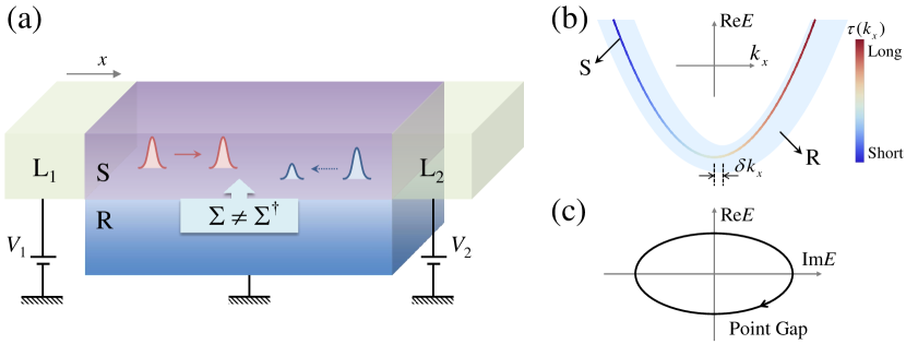
Figure 1: Proposed heterojunction composed of the system (S) coupled to a reservoir (R), the latter introducing a non-Hermitian self-energy $\Sigma\neq\Sigma^{\dagger}$ to S. Two leads $\text{L}_{1}$ and $\text{L}_{2}$ are coupled only to S and another lead (not shown) is coupled to R. Due to the reservoir-engineered non-Hermiticity, the propagation of wave packet in S exhibits nonreciprocity in the $x$-direction, i.e., the wave packet propagating leftward decays much faster than that propagating rightward. (b) Complex band structure in S (colored line) with the electron lifetime denoted by the color. A relative momentum shift $\delta k_{x}$ between the band of S and that of R (shadow region) leads to asymmetric coupling between them. (c) Complex energy spectrum with the point gap topology.

In this paper, we propose to engineer and detect the NHSE in an electronic mesoscopic heterojunction, as shown in Fig. 1(a), which is composed of two parts: a system (S) and a reservoir (R), coupled to each other. Due to the coherent coupling, S becomes non-Hermitian, and can be effectively described by the Green’s function as

$$\begin{split}\bm{g}^{r}(\omega)=\frac{1}{\omega-H_{\text{eff}}(\omega)},\ \ H_{\text{eff}}(\omega)=H_{\text{S}}+\Sigma^{r}_{\text{R}}(\omega),\end{split}$$ (1)

where the effective Hamiltonian $H_{\text{eff}}$ of S consists of the bare Hamiltonian $H_{\text{S}}$ and the retarded self-energy $\Sigma^{r}_{\text{R}}(\omega)$ due to the coupling between S and R. The self-energy is in general non-Hermitian with $\Sigma^{r}_{\text{R}}\neq\Sigma_{\text{R}}^{r{\dagger}}$; see Fig. 1(a). Given that the dynamics of the electrons in S is governed by the Green’s function $\bm{g}^{r}$ or equivalently, the effectively Hamiltonian $H_{\text{eff}}$ in Eq. (1), very interesting non-Hermitian effects can be implemented in S by properly engineered $\Sigma_{\text{R}}^{r}$. Here, we focus on the special type of $\Sigma_{\text{R}}^{r}$ that can give rise to the NHSE. If S is coupled to R asymmetrically for $k_{x}>0$ and $k_{x}<0$ in Fig. 1(b), there will be unequal lifetimes of electrons in S moving forward and backward. The resultant $H_{\text{eff}}$ yields a point gap topology in its complex spectrum under the PBC [Fig. 1(c)], and accordingly, the wave functions under the OBC exhibit the NHSE [Figs. 2(d-f)], which can be well described by the generalized Brillouin zone (GBZ) [Fig. 2(c)].

The great advantage of our proposal is that the non-Hermitian phenomena can be probed by the standard transport measurements. To achieve this, two leads L_1,2 in Fig. 1(a) are designed to connect only to S so that the current flowing between them provides a direct measure of the non-Hermitian effects in S. Moreover, such non-Hermitian physics in S can be incorporated straightforwardly into the framework of non-equilibrium Green’s function theory for quantum transport Datta (1995). We will show that the point gap topology of the complex spectrum gives rise to nonreciprocal charge transport between L₁ and L₂. Such a non-Hermitian scenario can be generalized to the spin-resolved situation and lead to nonreciprocal spin transport.

The rest of the paper is organized as follows. In Sec. II and Sec. III, we show how to engineer both the conventional and spin-resolved NHSE in the 1D systems by coupling to the reservoir and discuss the resultant nonreciprocal charge and spin transport phenomena, respectively. In Sec. IV and Sec. V, the main results of the nonreciprocal charge and spin transport are generalized to 2D systems. Finally, some discussions and prospects are given in Sec. VI.

II Nonreciprocal charge transport in 1D system

To be concrete, we start with a 1D system arranged in the $x$-direction coupled to a reservoir, which simulates a nanowire deposited on a 2D substrate. Assuming the PBC in the $x$-direction, the whole system can be described by the following Hamiltonian (lattice constant set to unity) as

$$\begin{split}H&=H_{\text{S}}+H_{\text{R}}+H_{\text{T}},\\ H_{\text{S}}&=\sum_{k_{x}}\varepsilon_{s}(k_{x})c_{k_{x}}^{\dagger}c_{k_{x}},\ \ \ H_{\text{T}}=\sum_{k_{x}}\big{(}t_{0}c_{k_{x}}^{\dagger}a_{k_{x},0}+\text{H.c.}\big{)},\\ H_{\text{R}}&=\sum_{k_{x},y=0}^{y=-\infty}\big{[}\varepsilon_{r}(k_{x})a_{k_{x},y}^{\dagger}a_{k_{x},y}+(t_{r}^{y}a_{k_{x},y}^{\dagger}a_{k_{x},y-1}+\text{H.c.})\big{]}.\end{split}$$ (2)

Here, $\varepsilon_{s}(k_{x})=2t_{s}\cos k_{x}-U_{s}$ is the electronic energy in S measured from its band bottom $U_{s}$ with $t_{s}$ the hopping strength, $\varepsilon_{r}(k_{x})=2t_{r}^{x}\cos\left(k_{x}+\delta k_{x}\right)-U_{r}$ is the $x$-direction energy dispersion in R also measured from its band bottom $U_{r}$ with $t_{r}^{x}$ the relevant hopping strength, and $t_{r}^{y}$ is the $y$-direction hopping in R. $\delta k_{x}$ describes the deviation in momentum $k_{x}$ between the bands of S and R, which mimics the asymmetric band structures of S and R that generally exist for different materials, as shown in Fig. 1(b). The interface coupling $t_{0}$ ($\ll t^{y}_{r}$) takes place between S and the outmost layer of R. High quality of the interface is assumed such that the coupling between S and R ensures $k_{x}$ conservation. The Fermi operators $c_{k_{x}}$ and $a_{k_{x},y}$ correspond to S and R, respectively, the latter being written in the mixed reciprocal and real spaces for respective directions. The subscript $y=0,-1,\cdots,-\infty$, which simulates the R connected to another lead in the bottom [cf. Fig 1(a)].

By integrating out the reservoir part of Eq. (2), the effective Hamiltonian $H_{\text{eff}}(\omega)$ in S can be obtained, with the $k_{x}$-dependent retarded self-energy as [cf. Appendix B]

$$\begin{split}\Sigma^{r}_{\text{R}}(k_{x},\omega)&=\big{[}\epsilon-\text{sgn}(\epsilon+1)\sqrt{\epsilon^{2}-1}\big{]}t_{0}^{2}/t_{r}^{y},\\ \epsilon&=[\omega-\varepsilon_{r}(k_{x})]/(2t_{r}^{y}),\end{split}$$ (3)

where sgn($\cdot$) is the sign function. Negative imaginary part of the self-energy, $\text{Im}(\Sigma^{r}_{\text{R}})<0$, arises as $|\epsilon|<1$ due to the electronic coupling of S and R and accordingly, the energy $E=\varepsilon_{s}(k_{x})+\Sigma^{r}_{\text{R}}$ becomes complex. The condition means that for a given $k_{x}$, only those electron wave functions in S with energy $\omega$ satisfying $|\omega-\varepsilon_{r}|<2t_{r}^{y}$ decay with motion and at the same time appear in R through the interface. Here, the momentum difference $\delta k_{x}$ or more generally, the asymmetry in the bands of S and R is the key ingredient for engineering the NHSE. It leads to unequal decay of the $\pm k_{x}$ states in S with $\text{Im}[E(k_{x},\omega)]\neq\text{Im}[E(-k_{x},\omega)]$ and so breaks the reciprocity; see Figs. 2(a) and 2(b). The inverse lifetime of electrons in S is given by $\tau^{-1}(k_{x},\omega)=-\text{Im}[E(k_{x},\omega)]$, which is proportional to velocity $v^{R}_{y}(k_{x},\omega)$ along the $y$ direction of electrons in R [cf. Appendix B].

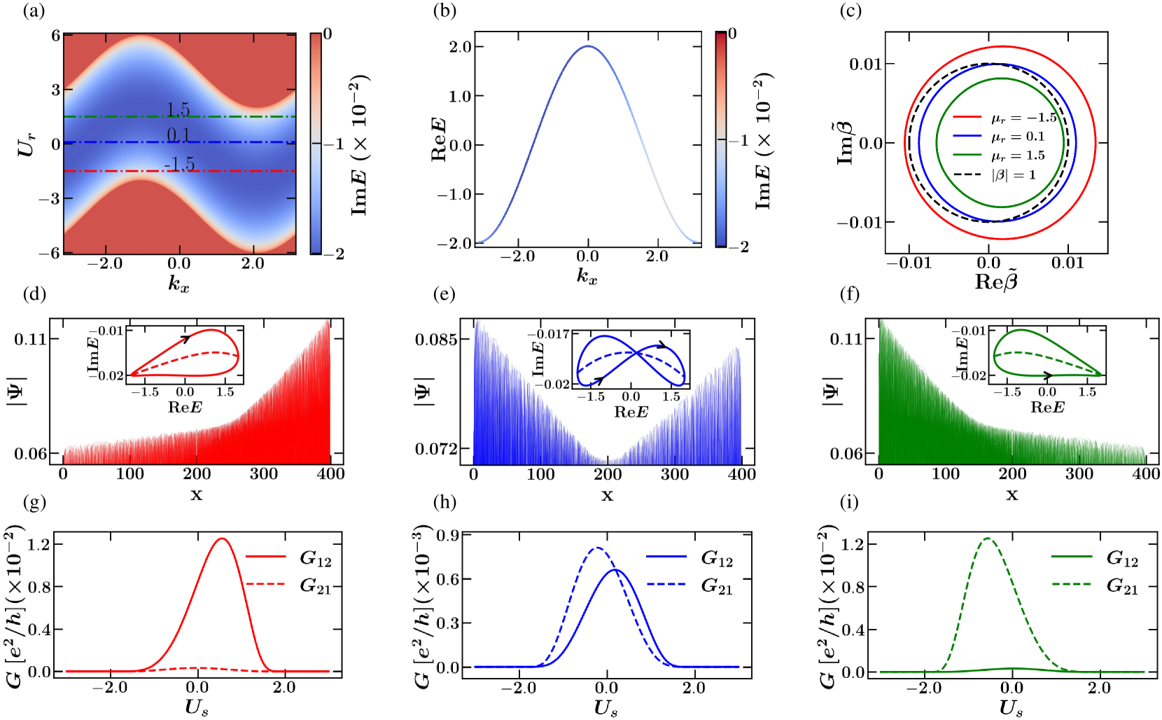
Figure 2: (a) $\text{Im}E$ as a function of $U_{r}$ and $k_{x}$, which contains the information of the electron lifetime in S. (b) Complex energy band with $U_{r}=1.5$ and $U_{s}=0$, whose imaginary part is shown by the color. (c) GBZs calculated by the effective Hamiltonian $H_{\text{eff}}$ of S for $U_{r}=\pm 1.5,0.1$ denoted in (a), in which $\tilde{\beta}=(|\beta|-0.99)e^{i\text{Arg}[\beta]}$. (d-f) Normalized eigenfunctions under OBC for various $U_{r}$ corresponding to those in (c). Insets: Complex spectral winding under PBC (solid line) and energy spectrum under OBC (dashed line) with $U_{s}=0$. (g-i) Zero-bias differential conductance as a function of $U_{s}$ that corresponds to the non-Hermitian properties in (d-f), respectively. Other parameters are $\omega=0$, $t_{s}=t_{r}^{x}=1$, $t^{y}_{r}=2.01$, $t_{0}=0.1t_{r}^{y}$ and $\delta k_{x}=\pi/3$. For the results calculated under the OBC, the length of the system in the $x$ direction is $L=400$.

In what follows we focus on quantum transport at zero bias ($\omega=0$). In Fig. 2(a) we show $\text{Im}E$ as a function of $k_{x}$ and $U_{r}$ with $t_{r}^{y}>t_{r}^{x}$. It is found that there are two types of non-Hermitian regions. In region (i) of $|U_{r}|<2(t_{r}^{y}-t_{r}^{x})$, $E(k_{x})$ is entirely complex for all $k_{x}$ states and there appears nontrivial winding [insets of Figs. 2(d-f)]. If $t_{r}^{y}<t_{r}^{x}$, there will be no such a full complex-spectrum region. In region (ii) of $|U_{r}|\in 2(t_{r}^{y}-t_{r}^{x},t_{r}^{y}+t_{r}^{x})$, complex energy spectrum appears only for a subset of $k_{x}$ states, in which there still be a point gap. In both non-Hermitian regions, electrons in S moving forward and in the opposite direction have unequal lifetimes, which leads to the NHSE. On the contrary, for $|U_{r}|>2(t_{r}^{y}+t_{r}^{x})$, no electron in S can enter R so that there is no NHSE.

It is known that the ways of spectral winding under the PBC determine the properties of the skin modes under the OBC Okuma et al. (2020); Zhang et al. (2020). To investigate the NHSE, we rewrite Hamiltonian (2) of the whole system in both directions in real space and calculate the self-energy of S by solving the surface Green’s function of R numerically [cf. Appendix C]. The effective Hamiltonian of S reads $H_{\text{eff}}^{\text{latt}}=\sum_{i,j}t_{ji}c^{\dagger}_{j}c_{i}$ with $t_{ji}$ the dressed hopping from site $i$ to $j$. Different from $H_{\text{S}}$, $H_{\text{eff}}^{\text{latt}}$ involves long-range hopping. In the non-Hermitian regions (i, ii), we have $H^{\text{latt}}_{\text{eff}}\neq H^{\text{latt}{\dagger}}_{\text{eff}}$, since the hopping terms of $t_{ji}\neq t^{*}_{ij}$ break the reciprocity. The eigenfunctions $\Psi$ of $H^{\text{latt}}_{\text{eff}}$ are numerically solved under the OBC in the $x$-direction, as shown in Figs. 2(d-f), exhibiting obvious NHSE. The full complex spectrum in region (i) indicate that all eigenstates under the OBC are the skin modes. The location where these skin modes pile up is determined by the specific way of the spectral winding, as shown in insets of Figs. 2(d-f) with arrows representing the direction in which $k_{x}$ increases. The clockwise and anti-clockwise winding takes place for different $U_{r}$, and correspond to the skin patterns stacked on the right and left boundaries, respectively; see Figs. 2(d) and 2(f). There also exists interesting “$\infty$”-shaped winding Okuma et al. (2020); Zhang et al. (2020), which gives rise to the skin modes stacked simultaneously on both boundaries, see Fig. 2(e). The skin patterns obtained above are consistent with the description by the GBZ Yao and Wang (2018) in Fig. 2(c) [cf. Appendix D]. In region (ii), the nontrivial winding persists for the complex energy spectrum [cf. Appendix E].

Compared with the energy spectrum, more information is involved in the complex band structure shown in Fig. 2(b). Specifically, its real and imaginary parts will determine the quantum transport taking place in S. The asymmetric band structures result in nonreciprocal transport in S, which is embodied in the effective Hamiltonian $H_{\text{eff}}$ or the Green’s function $\bm{g}^{r}$. Such an effective description can be incorporated into the framework of the non-equilibrium Green’s function method to study the transport properties. The differential conductance between leads L_1,2 is defined as Datta (1997)

$$\begin{split}&G_{\alpha\beta}(eV)=\frac{\partial I_{\beta}}{\partial V_{\alpha}}=\frac{e^{2}}{h}\text{Tr}\big{[}\bm{\Gamma}_{\beta}\textbf{G}^{r}\bm{\Gamma}_{\alpha}\textbf{G}^{a}\big{]}_{\omega=eV},\\ &\textbf{G}^{r,a}=\bm{g}^{r,a}+\sum_{\alpha=1,2}\bm{g}^{r,a}\Sigma_{\alpha}^{r,a}\textbf{G}^{r,a},\bm{\Gamma}_{\alpha}=i(\Sigma_{\alpha}^{r}-\Sigma_{\alpha}^{a}),\end{split}$$ (4)

where subscripts $\alpha,\beta=1,2$ indicate the lead labels. The full retarded (advanced) Green’s function $\textbf{G}^{r}$ ($\textbf{G}^{a}$) can be solved by the Dyson equation with self-energy $\Sigma_{\alpha}^{r,a}$ and corresponding linewidth function $\bm{\Gamma}_{\alpha}$ due to the coupling with lead L_α.

The NHSE can be detected by the transport signatures between leads L₁ and L₂. The zero-bias differential conductance $G_{\alpha\beta}$ is calculated by Eq. (4) on the discrete lattices and its dependence on $U_{s}$ is plotted in Figs. 2(g-i). The one-to-one (up-to-down) correspondence between Figs. 2(g-i) and Figs. 2(d-f) can be easily understood physically. The zero-bias conductance for a given $U_{s}$ reflects the information at the Fermi level so that the nonreciprocal conductance varying with $U_{s}$ can be regarded as a complex spectral tomography. Although the skin modes are not completely stacked at the boundary, somewhat different from those in simple non-Hermitian lattices Yao and Wang (2018), the conductance in Figs. 2(g,i) exhibits a strong nonreciprocity with the current flowing in one direction being much greater than that in the opposite direction. Such a diode-like effect stems from the unequal lifetimes of electronic states with opposite momentum, or equivalently, the point gap topology [cf. Fig. 1]. The degree of nonreciprocity, i.e., the ratio between the current flowing in the two opposite directions enhances as the length of the system becomes larger. The forward direction of the diode is determined by the ways of spectral winding in Figs. 2(d,f), which is also consistent with the direction in which the skin modes are stacked. For the simple winding, nonreciprocal transport with the same forward direction takes place for all energies. On the other hand, the “$\infty$”-shaped winding in Fig. 2(e) results in an energy-dependent nonreciprocity, see Fig. 2(h). Specifically, the curves of $G_{12}$ and $G_{21}$ intersect at the energy just corresponding to the crossing point of the “$\infty$”-spectrum, as shown in Figs. 2(e) and 2(h). In this case, the nonreciprocal transport effect is greatly reduced due to the nearly equal $G_{12}$ and $G_{12}$. The above discussion focuses on the non-Hermitian region (i). In region (ii), both nonreciprocal and reciprocal transport can be realized in different energy windows [cf. Appendix E].

Note that the non-Hermitian physics in S is embodied in self-energy $\Sigma_{\text{R}}^{r}$ induced by the coupling to R. From a mathematical point of view, the calculation of $\Sigma_{\text{R}}^{r}$ and $\Sigma_{1,2}^{r}$ induced by L_1,2 is on an equal footing. Therefore, the conductance can be calculated in a conventional way Datta (1997) by regarding the whole setup (S+R) in Fig. 1(a) as a scattering region connecting to three terminals, which ensures the correctness of our results. Physically, however, the two types of self-energies play distinctive roles: proper engineering of $\Sigma_{\text{R}}^{r}$ yields interesting non-Hermitian effect while leads L_1,2 are just used for its detection.

III Nonreciprocal spin transport in 1D system

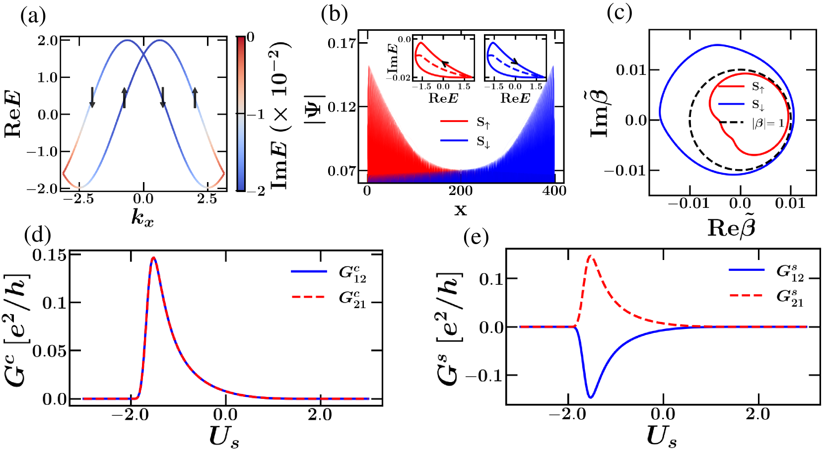
Figure 3: (a) Spinful complex energy bands with the arrows denoting the spin polarizations. (b) Skin modes and spectral winding (insets). (c) GBZs for both spins. (d) Charge and (e) spin conductance as a function of $U_{s}$. The parameters are $\omega=0$, $\delta k_{x}=0$, $U_{r}=1.5$ and $\delta k^{\prime}_{x}=\pi/5$ with the others the same as those in Fig. 2.

The scenario of the NHSE in heterostructures can be generalized straightforwardly to the spin-resolved case. Let’s replace $H_{\text{S}}$ in Eq. (2) by

$$\tilde{H}_{\text{S}}=\sum_{k_{x},\sigma=\uparrow,\downarrow}\varepsilon_{s}^{\sigma}\left(k_{x}\right)c^{\dagger}_{k_{x},\sigma}c_{k_{x},\sigma}~{},$$ (5)

where $\varepsilon_{s}^{\sigma}\left(k_{x}\right)=2t_{s}\cos\left(k_{x}+\delta k_{x}^{\sigma}\right)-U_{s}$ is the dispersion for electrons with spin $\sigma$. The opposite shift of the momentum $\delta k_{x}^{\uparrow,\downarrow}=\mp\delta k^{\prime}_{x}$ for the two spin states can be induced by the Rashba spin-orbit coupling. $H_{\text{R}}$ and $H_{\text{T}}$ are the same as those in Eq. (2) except that the spin degeneracy in R is now considered and $\delta k_{x}=0$ is taken. Note that only the relative momentum shift of the bands, rather than their absolute values, has physical effects.

From the effective Hamiltonian $\tilde{H}_{\text{eff}}$ of S, we numerically obtain spin-dependent complex band structures, as shown in Figs. 3(a). The time-reversal symmetry ensures to have an equal lifetime for the states with opposite momentum and spin, $i.e.$, $\tau_{\uparrow}(k_{x},\omega)=\tau_{\downarrow}(-k_{x},\omega)$. The picture shown in Fig. 3(a) indicates that the spin splitting of the bands will lead to spin-resolved nonreciprocity. Accordingly, the NHSE becomes spin dependent in Fig. 3(b), where the spectral winding and the skin-mode accumulation occur in opposite directions for opposite spin polarizations, which is also verified by the GBZs in Fig. 3(c). The above picture predicts reciprocal transport for charge but nonreciprocal transport for spin. The charge conductance $G_{ij}^{c}=G_{ij}^{\uparrow}+G_{ij}^{\downarrow}$ and spin conductance $G_{ij}^{s}=G_{ij}^{\uparrow}-G_{ij}^{\downarrow}$ are plotted in Figs. 3(d,e). It is found that two different spin states have equal contribution to $G_{ij}^{c}$, but opposite contribution to $G_{ij}^{s}$. The predicted transport properties are manifested as $G_{12}^{c}=G_{21}^{c}$ and $G_{12}^{s}=-G_{21}^{s}$. Such nonreciprocal spin transport can be used as a spin filter with the spin polarization being controlled conveniently by the current direction.

IV Nonreciprocal charge transport in 2D systems and magnetic field effect

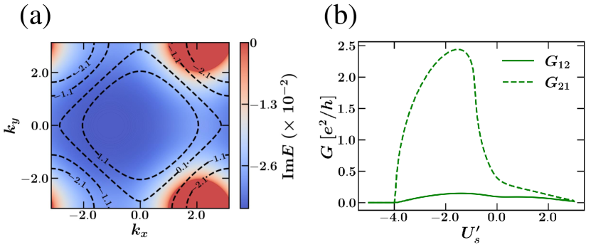
Figure 4: (a) $\text{Im}E$ as a function of $k_{x}$ and $k_{y}$ with the dashed lines being the $\text{Re}E$ contours ($E$ is the eigenvalue of $H_{\text{eff}}^{\text{2D}}$ in Eq. (7)). (b) Zero-bias differential conductance as a function of $U_{s}^{\prime}$. The relevant parameters are $U_{r}^{\prime}=4.1$, $\omega=0$, $t_{r}^{\prime x}=t_{r}^{\prime y}=t_{s}^{\prime}=1$, $t_{r}^{\prime z}=3.5$, $t_{0}^{\prime}=0.1t_{r}^{\prime z}$, $B=0$ and $\Delta k_{x}=\pi/3$. The length ($x$ direction) and width ($y$ direction) are $L=100$ and $W=200$, respectively.

The general scenario of the reservoir-engineered NHSE and the resultant nonreciprocal transport is not restricted to a specific spatial dimension. In this section, we show that nonreciprocal charge transport can be implemented in 2D heterostructures as well. We adopt the following lattice Hamiltonian

$$\begin{split}H_{\text{S}}^{\text{2D}}&=\sum_{x,y}\big{(}t_{s}^{\prime}c_{x+1,y}^{\dagger}c_{x,y}+t_{s}^{\prime}e^{iBx}c_{x,y+1}^{\dagger}c_{x,y}-\frac{U_{s}^{\prime}}{2}c_{x,y}^{\dagger}c_{x,y}+\text{H.c.}\big{)},\ \ \ H_{\text{T}}^{\text{2D}}=\sum_{x,y}\big{(}t_{0}^{\prime}c_{x,y}^{\dagger}a_{x,y,z=0}+\text{H.c.}\big{)},\\ H_{\text{R}}^{\text{2D}}&=\sum_{x,y,z=0}^{z=-\infty}\big{(}t_{r}^{\prime x}e^{i\Delta k_{x}}a_{x+1,y,z}^{\dagger}a_{x,y,z}+t_{r}^{\prime y}e^{iBx}a_{x,y+1,z}^{\dagger}a_{x,y,z}+t_{r}^{\prime z}a_{x,y,z+1}^{\dagger}a_{x,y,z}-\frac{U_{r}^{\prime}}{2}a_{x,y,z}^{\dagger}a_{x,y,z}+\text{H.c.}\big{)},\\ \end{split}$$ (6)

where $t_{s}^{\prime}$ is the hopping in the system and $t_{r}^{\prime x},t_{r}^{\prime y},t_{r}^{\prime z}$ are those in the reservoir, $U_{s}^{\prime}$ and $U_{r}^{\prime}$ are the energies of the band bottoms, $t_{0}^{\prime}$ is the interface coupling, and the momentum deviation $\Delta k_{x}$ again mimics the asymmetric band structures. For the later study of the magnetic field effect, we have also introduced a magnetic field $B$ in the $z$ direction, which is reflected in the phase factor $e^{iBx}$.

Without a magnetic field, Hamiltonian (6) has translational invariance in both the $x$ and $y$ directions. Similar to the 1D case, we solve the effective Hamiltonian for the system under the PBC in both directions as

$$\begin{split}&H_{\text{eff}}^{\text{2D}}(\omega,\mathbf{k})=2t^{\prime}_{s}\cos(k_{x})+2t^{\prime}_{s}\cos(k_{y})-U_{s}^{\prime}+\Sigma^{\prime r}_{\text{R}}(\omega,\mathbf{k})~{},\\ &\Sigma^{\prime r}_{\text{R}}=\Big{[}\epsilon^{\prime}-\text{sgn}\left(\epsilon^{\prime}+1\right)\sqrt{\epsilon^{\prime 2}-1}\Big{]}t_{0}^{\prime 2}/t_{r}^{\prime z},\\ &\epsilon^{\prime}=\big{[}\omega+U^{\prime}_{r}-2t_{r}^{\prime x}\cos(k_{x}+\Delta k_{x})-2t_{r}^{\prime y}\cos(k_{y})\big{]}/(2t_{r}^{\prime z}).\end{split}$$ (7)

In Fig. 4(a), we plot $\text{Im}E$ as a function of $k_{x}$ and $k_{y}$. One can see that although the Fermi surface of the system is symmetric about $k_{x}=0$, $\text{Im}E$ does not. As a result, nonreciprocal charge transport takes place which is manifested as $G_{12}\neq G_{21}$ in Fig. 4(b).

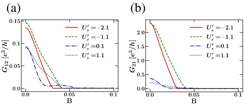
Figure 5: Conductance as a function of the magnetic field $B$. The parameters are the same as those in Fig. 4.

It has been known that a magnetic field will strongly suppress the non-Hermitian skin effect in 2D systems Shao et al. (2022); Lu et al. (2021). In Fig. 5, we plot the conductance as a function of the magnetic field. One can see that a small magnetic field strongly suppresses both $G_{12}$ and $G_{21}$ and so the nonreciprocal charge transport disappears. The sensitivity of the non-Hermitian skin effect to the magnetic field provides an effective way for the control of the nonreciprocal charge transport in 2D heterojunctions.

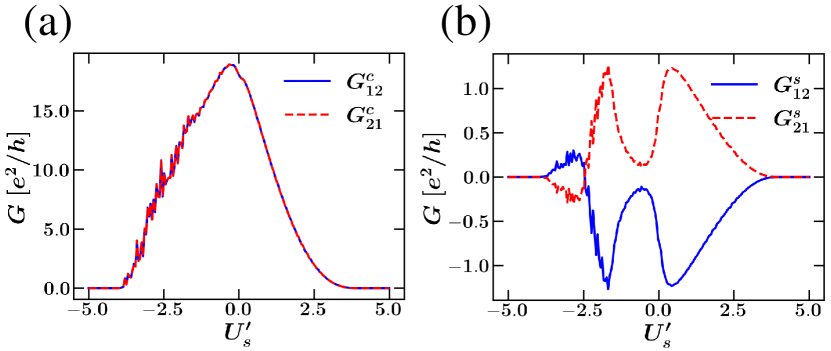
Figure 6: (a) Charge and (b) spin conductance as a function of $U_{s}^{\prime}$. The parameters are $t_{r}^{\prime z}=3.1,t_{0}^{\prime}=0.1t_{r}^{\prime z},t_{soc}=0.2,L=W=40$ and the others are the same as those in Fig. 4

V Nonreciprocal spin transport in 2D systems

In this section, we investigate nonreciprocal spin transport in 2D systems. Similar to the 1D case, we consider the system to be the 2D electron gas with Rashba spin-orbit coupling, which is described by the Hamiltonian

$$\begin{split}\tilde{H}_{\text{S}}^{2\text{D}}&=\sum_{\bm{k}}c^{\dagger}_{\bm{k}}h_{s}(\bm{k})c_{\bm{k}},\\ h_{s}(\bm{k})&=\tilde{\varepsilon}_{s}(\bm{k})+2t_{soc}(\sin k_{x}\sigma_{y}-\sin k_{y}\sigma_{x}),\end{split}$$ (8)

where $\tilde{\varepsilon}_{s}(\bm{k})=2t_{s}(\cos k_{x}+\cos k_{y})-U_{s}^{\prime}$ , $t_{soc}$ is the spin dependent hopping due to the Rashba spin-orbit coupling, the Fermi operator $c_{\bm{k}}=(c_{\bm{k}}^{\uparrow},c_{\bm{k}}^{\downarrow})^{\text{T}}$ has two spin components and Pauli matrices $\sigma_{x,y}$ act on the spin. $H_{\text{R}}^{\text{2D}}$ and $H_{\text{T}}^{\text{2D}}$ are the same as those in Eq. (6) except that the spin degeneracy in the reservoir is now considered and $\Delta k_{x}=0$ and $B=0$ are taken. The self-energy $\Sigma^{\prime r}_{\text{R}}$ due to the reservoir is the same as that in Eq. (7) with $\Delta k_{x}=0$. Here, $\text{Im}E$ is symmetric about $k_{x}=0$ but instead, the bare Hamiltonian (8) possesses a spin dependent band splitting, which yields reciprocal charge transport but nonreciprocal spin transport, similar to the 1D case. Given the specific spin texture of the 2D electron gas, the nonreciprocity that occurs in the $x$ direction should be most visibly revealed by the spin current defined with its polarization along the $y$ direction. The corresponding conductance is denoted by $G_{ij}^{\rightarrow}$ and $G_{ij}^{\leftarrow}$, whose superscripts $\rightarrow,\leftarrow$ mean the spin components along the $y,-y$ directions, respectively. In Fig. 6, we plot the charge conductance $G_{ij}^{c}=G_{ij}^{\rightarrow}+G_{ij}^{\leftarrow}$ and spin conductance $G_{ij}^{s}=G_{ij}^{\rightarrow}-G_{ij}^{\leftarrow}$. The same as the 1D case, two different spin states have equal contribution to $G_{ij}^{c}$, but opposite contribution to $G_{ij}^{s}$. The predicted transport properties are again manifested as $G_{12}^{c}=G_{21}^{c}$ and $G_{12}^{s}=-G_{21}^{s}$. Interestingly, the nonreciprocal spin current can have opposite sign in different energy regions, which stems from the rich spin texture of the 2D Rashba gas compared with that in the 1D case.

VI Discussions and prospects

We discuss the experimental implementation of our proposal. The main ingredients, mesoscopic heterostructures with multiple terminals, are common setups studied in mesoscopic physics Datta (1997), which can be fabricated with mature technology. To achieve the NHSE, materials with proper band structures and good tunability by external fields are favorable. For the spinless NHSE and nonreciprocal charge transport, the time-reversal symmetry must be broken. In our example described by Eqs. (2) and (6), such a symmetry breaking is introduced by a relative momentum shift $\delta k_{x}$ (or $\Delta k_{x}$) for clarity. In reality, any band structures of S and R that lead to unequal lifetimes of electrons counter-propagating in S are sufficient for the NHSE. For example, the study of the heterostructures of topological matter has shown that their band structures have strong external field tunability Mourik et al. (2012); Yuan and Fu (2018), so that both nonreciprocal charge and spin transport is expected to be realized in these systems. Moreover, the coexistence of the Rashba spin-orbit coupling and a Zeeman field in the 2D electron systems can also give rise to an asymmetric coupling to the reservoir and the resultant NHSE Tokura and Nagaosa (2018); Bihlmayer et al. (2022). For the spin-resolved NHSE, the time-reversal symmetry does not need to be broken so that the Rashba spin-orbit coupling is sufficient for such an effect and the resultant nonreciprocal spin transport. Finally, we remark that the engineering of the NHSE in mesoscopic systems can be further extended to other scenarios including electron-electron, electron-phonon, electron-impurity scattering and so on Nagai et al. (2020); Papaj et al. (2019); Kozii and Fu (2017); Shen and Fu (2018). Regardless of different physical origins, the NHSE in the electron systems can be probed by the transport measurement schemes proposed in this work.

In this paper, we construct the lattice model, calculate the self-energy and transport properties using the KWANT package Groth et al. (2014).

Appendix A Surface Green’s function of the reservoir

To arrive at the retarded self-energy induced by the semi-infinite reservoir, we follow the procedure in Ref. Wimmer (2009). The Hamiltonian of the reservoir can be rewritten in the general form of

$$H_{\text{R}}=\sum_{y=0}^{-\infty}a_{y}^{\dagger}H_{0}a_{y}+a_{y-1}^{\dagger}H_{-1}a_{y}+a_{y}^{\dagger}H_{1}a_{y-1},$$ (9)

where only the $y$ coordinate is shown in the subscript of the Fermi operator $a_{y}$. Under the open boundary condition (OBC) in the $x$ direction, $a_{y}$ is a vector written in real space as $a_{y}=(a_{x=1,y},a_{x=2,y},\cdots,a_{x=L,y})^{\text{T}}$; while under the periodic boundary condition (PBC), the eigenstates in the $x$ direction can be labeled by $k_{x}$ and so $a_{y}=a_{k_{x},y}$. The sites of $y=0$ are the outmost layer of the reservoir that are coupled to the system. The matrices $H_{0}$ and $H_{\pm 1}$ are the unit-cell Hamiltonian and the hopping Hamiltonian of the reservoir, respectively. Both $H_{0}$ and $H_{\pm 1}$ are $N_{\text{u.c. }}\times N_{\text{u.c. }}$ square matrices, with $N_{\text{u.c.}}=L$ ($L$ the length of the system in the $x$ direction) under the OBC and $N_{\text{u.c. }}=1$ under the PBC, respectively.

We denote the retarded Green’s function of the reservoir by $g^{r}$ and the surface Green’s function $\mathcal{G}^{r}_{\text{R}}=g_{00}^{r}$ is just the matrix element for the outmost layer. To obtain $\mathcal{G}^{r}_{\text{R}}$, we need to solve the quadratic eigenvalue equation

$$\left(\left(\omega-H_{0}\right)\lambda_{n}-H_{1}\lambda_{n}^{2}-H_{-1}\right)\bm{u}_{n}=0~{},$$ (10)

for a given $\omega$, where $\bm{u}_{n}$ is the right eigenvector corresponding to the eigenvalue $\lambda_{n}$. We also need to calculate the group velocity $v_{n}$ of the Bloch modes given by

$$v_{n}=-\frac{1}{\hbar}\text{Im}\left(2\bm{u}_{n}^{\dagger}H_{1}\lambda_{n}\bm{u}_{n}\right)~{}.$$ (11)

Solving the quadratic eigenproblem in Eq. (10) yields $2N_{\text{u.c.}}$ eigenvalues and eigenvectors, which can be divided into two groups:

• $N_{\text{u.c.}}$ modes moving in the $-y$ direction with $\left|\lambda_{n}\right|<1$ or $\left|\lambda_{n}\right|=1\wedge v_{n}>0$. These eigenvalues are denoted by $\lambda_{n,<}$ and the corresponding eigenvectors are $\bm{u}_{n,<}$ which we collect into the matrix $U_{<}=\left(\bm{u}_{1,<},\ldots,\bm{u}_{N_{\text{u.c. }},<}\right)$.

• $N_{\text{u.c.}}$ modes moving in the $y$ direction with $\left|\lambda_{n}\right|>1$ or $\left|\lambda_{n}\right|=1\wedge v_{n}<0$. These eigenvalues are denoted by $\lambda_{n,>}$ and the corresponding eigenvectors are $\bm{u}_{n,>}$ which we collect into the matrix $U_{>}=\left(\bm{u}_{1,>},\ldots,\bm{u}_{N_{\text{u.c. }},>}\right)$.

Then the surface Green’s function can be solved by

$$\mathcal{G}^{r}_{\text{R}}H_{-1}=U_{<}\Lambda_{<}U_{<}^{-1}~{},$$ (12)

and if $H_{-1}$ is invertible we have

$$\mathcal{G}^{r}_{\text{R}}=U_{<}\Lambda_{<}U_{<}^{-1}H_{-1}^{-1}~{},$$ (13)

where $\Lambda_{<}=\left(\begin{array}[]{cccc}\lambda_{1,<}&&&0\\ &\lambda_{2,<}&&\\ &&\ddots&\\ 0&&&\lambda_{N_{\text{u.c. }},<}\\ \end{array}\right)$ is the diagonal matrix composed of the eigenvalues $\lambda_{n,<}$. With the surface Green’s function, the retarded self-energy can be obtained as

$$\Sigma^{r}_{\text{R}}=t_{0}^{2}\mathcal{G}^{r}_{\text{R}}~{},$$ (14)

where $t_{0}$ is the coupling strength between the reservoir and the system.

Table 1: A submatrix of $H^{\text{latt}}_{\text{eff}}$ with the diagonal elements being the onsite potential and the upper and lower diagonal elements being the nearest-neighbor hopping. The relevant parameters are the same as those in Fig. 2 and $U_{r}=1.5$.

$7.50\times 10^{-3}-1.69\times 10^{-2}i$	$1.00-5.51\times 10^{-3}i$	$-8.03\times 10^{-4}-4.64\times 10^{-4}i$	$1.37\times 10^{-4}i$
$1.00+3.15\times 10^{-3}i$	$7.50\times 10^{-3}-1.69\times 10^{-2}i$	$1.00-5.51\times 10^{-3}i$	$-8.03\times 10^{-4}-4.64\times 10^{-4}i$
$8.03\times 10^{-4}-4.64\times 10^{-4}i$	$1.00+3.15\times 10^{-3}i$	$7.50\times 10^{-3}-1.69\times 10^{-2}i$	$1.00-5.51\times 10^{-3}i$
$1.37\times 10^{-4}i$	$8.03\times 10^{-4}-4.64\times 10^{-4}i$	$1.00+3.15\times 10^{-3}i$	$7.50\times 10^{-3}-1.69\times 10^{-2}i$

Appendix B Derivation of Eq. (3) and the lifetime

Under the PBC in the $x$ direction, we have $H_{0}=2t_{x}\cos(k_{x}+\Delta k_{x})-U_{r}$ and $H_{1}=H_{-1}=t_{r}^{y}$ in Eq. (9), making use of the good quantum number $k_{x}$. The quadratic eigenproblem reduces to

$$\lambda^{2}-2\epsilon\lambda+\epsilon^{2}=\epsilon^{2}-1~{},$$ (15)

$$\epsilon(k_{x},\omega)=\frac{\omega+U_{r}-2t_{r}^{x}\cos(k_{x}+\Delta k_{x})}{2t_{r}^{y}}~{},$$

which yields two roots of $\lambda$:

$$\lambda_{\pm}=\epsilon\pm\sqrt{\epsilon^{2}-1}~{}.$$ (16)

Without loss of generality, $t_{r}^{x,y}$ are chosen to be real and so is $\epsilon$. If $|\epsilon|\leq 1$, the roots contain an imaginary part so that $|\lambda_{\pm}|=1$, which corresponds to the propagating modes in the reservoir. To get the retarded surface Green’s function, we need to pick up those modes propagating in the $-y$ direction by their group velocity. Here, the group velocity in Eq. (11) reduces to

$$v_{\pm}=-\frac{1}{\hbar}\text{Im}\left(2t_{r}^{y}\lambda_{\pm}\right)~{},$$ (17)

and for $t_{r}^{y}>0$, $\lambda_{-}$ corresponds to the outgoing modes that we want. Then the retarded surface Green’s function of the reservoir is

$$\mathcal{G}^{r}_{{\text{R}}}=\lambda_{-}/t_{r}^{y}~{}.$$ (18)

If $|\epsilon|>1$, the roots are real numbers, and only those evanescent modes with $|\lambda|<1$ are relevant. In this case, the surface Green’s function can be expressed as

$$\mathcal{G}^{r}_{{\text{R}}}=\lambda_{\text{sgn}(-\epsilon)}/t_{r}^{y}~{}.$$ (19)

Inserting $\mathcal{G}^{r}_{{\text{R}}}$ into Eq. (14) yields the self-energy

$$\Sigma^{r}_{\text{R}}(k_{x},\omega)=\begin{cases}\left(\epsilon-\text{sign}\left(\epsilon\right)\sqrt{\epsilon^{2}-1}\right)t_{0}^{2}/t_{r}^{y}&|\epsilon|\geq 1~{},\\ \left(\epsilon-i\sqrt{1-\epsilon^{2}}\right)t_{0}^{2}/t_{r}^{y}&|\epsilon|<1~{},\end{cases}$$ (20)

which can be incorporated into the unified form of Eq. (3).

From Eqs. (14) (17) and (18), one can obtain the relation between the lifetime of the quasiparticle in the system and the velocity in the reservoir as

$$\frac{1}{\tau(k_{x},\omega)}=-\text{Im}\Big{[}\frac{\Sigma^{r}_{\text{R}}(k_{x},\omega)}{\hbar}\Big{]}=\frac{1}{2}\left(\frac{t_{0}}{{t_{r}^{y}}}\right)^{2}v_{y}^{R}(k_{x},\omega)~{},$$ (21)

where $v_{y}^{\text{R}}=v_{-}$. One can see that the lifetime of the quasiparticle in the system is inversely proportional to the electron velocity along the $y$ direction in the reservoir.

Appendix C Retarded self-energy in real space and nonreciprocal hopping

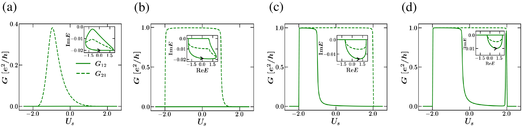
Figure 7: Comparison between the transport properties and complex spectrum [insets] in (a) non-Hermitian region (i) and (b-d) non-Hermitian region (ii). $U_{r}=2.0,3.0,5.0,5.5$ in (a-d), respectively. The other parameters are the same as those in Fig. 2.

Under the OBC, the matrices $H_{0}$, $H_{\pm 1}$ in Eq. (9) are

$$\begin{split}H_{0}&=\left(\begin{array}[]{cccc}-U_{r}&t_{r}^{x}&0&\cdots\\ t_{r}^{x}&-U_{r}&t_{r}^{x}&\cdots\\ \vdots&\vdots&\vdots&\vdots\\ \cdots&0&t_{r}^{x}&-U_{r}\end{array}\right)_{{L}\times{L}},\\ H_{\pm 1}&=\left(\begin{array}[]{cccc}t_{r}^{y}&0&0&\cdots\\ 0&t_{r}^{y}&0&\cdots\\ \vdots&\vdots&\vdots&\vdots\\ \cdots&0&0&t_{r}^{y}\end{array}\right)_{{L}\times{L}},\end{split}$$ (22)

with $L$ the length of the lattice in the $x$ direction. Following the procedure illustrated in Sec. A, we obtain the retarded self-energy matrix $(\Sigma_{\text{R}}^{r})_{{L}\times{L}}$ under the OBC. Combining the bare lattice Hamiltonian of the system,

$$H_{\text{S}}^{\text{latt}}=\left(\begin{array}[]{cccc}-U_{s}&t_{s}&0&\cdots\\ t_{s}&-U_{s}&t_{s}&\cdots\\ \vdots&\vdots&\vdots&\vdots\\ \cdots&0&t_{s}&-U_{s}\end{array}\right)_{{L}\times{L}}~{},$$ (23)

and the self-energy $(\Sigma_{\text{R}}^{r})_{{L}\times{L}}$ yields the effective non-Hermitian lattice Hamiltonian $H_{\text{eff}}^{\text{latt}}=H_{\text{S}}^{\text{latt}}+(\Sigma_{\text{R}}^{r})_{{L}\times{L}}$, which can be expressed in the general form $H_{\text{eff}}^{\text{latt}}=\sum_{i,j}t_{ji}c^{\dagger}_{j}c_{i}$. In the non-Hermitian regions (i, ii) discussed in Sec. II, we have $H^{\text{latt}}_{\text{eff}}\neq H^{\text{latt}{\dagger}}_{\text{eff}}$. For clarity, we exemplify the matrix elements of $H_{\text{eff}}^{\text{latt}}$ in Table  1, where the effective Hamiltonian contains long-range hopping and importantly, the hopping terms satisfying $t_{ji}\neq t^{*}_{ij}$ break the reciprocity and lead to the non-Hermitian skin effect.

Appendix D Calculation of the generalized Brillouin zone

The generalized Brillouin zone (GBZ) is the key concept of non-Bloch band theory, which provides an effective description of the non-Hermitian skin effect. Here, we illustrate the numerical procedure for the calculation of the GBZ following Refs. Yao and Wang (2018); Yang et al. (2020):

• Rewrite the eigenvalue equation $H_{\text{eff}}\left(\omega,k_{x}\right)-E=0$ into $H_{\text{eff}}\left(\omega,\beta\right)-E=0$ with the parameter defined by $\beta=e^{ik_{x}}$.

• Solve the eigenvalues $E_{\text{OBC}}$s of the lattice Hamiltonian $H_{\text{eff}}^{\text{latt}}$ under the OBC with $\omega=0$.

• Insert $E_{\text{OBC}}$ into the equation $H_{\text{eff}}\left(\omega,\beta\right)-E_{\text{OBC}}=0$ and find two roots $\beta_{1,2}$ of $\beta$ for each $E_{\text{OBC}}$. Plot all the roots on the complex plane, which give the GBZ in Fig. 2(c).

Appendix E Results for non-Hermitian region (ii)

For $t_{r}^{y}>t_{r}^{x}>0$, the system is in non-Hermitian region (ii) if $|U_{r}|\in 2(t_{r}^{y}-t_{r}^{x},t_{r}^{y}+t_{r}^{x})$, and for $t_{r}^{y}<t_{r}^{x}$, only non-Hermitian region (ii) exists. The main difference between the two non-Hermitian regions is that the energy spectrum in region (i) is entirely complex while that in region (ii) also contains real parts, which can be seen in Fig. 2(a). This fact is reflected by the spectral loop under the PBC, in which certain segments of the loop lie on the real axis; see Figs. 7(b-d). In those states with real energies, electrons can propagate without loss and give rise to quantized conductance; see $G_{21}$ in Figs. 7(b-d). Meanwhile, whether nonreciprocal transport takes place or not depends on the energy, which can still be inferred from the complex spectrum. Each energy $\text{Re}E$ has two states [$\pm k_{x}$ in Fig. 2(b)], which may split into two branches due to unequal $\text{Im}E$ and give rise to a point gap or may coincide at the real axis with $\text{Im}E=0$ for both states. For the former case, the conductance satisfies $G_{12}\neq G_{21}$ and exhibits strong nonreciprocity while for the latter case, one has $G_{12}=G_{21}$ and the nonreciprocity disappears; see the results in Figs. 7(c,d) in different energy regions.

References

- Dirac (1981) P. A. M. Dirac, The Principles of Quantum Mechanics (Clarendon Press, 1981).
- Breuer and Petruccione (2002) H.-P. Breuer and F. Petruccione, The theory of open quantum systems (Oxford University Press on Demand, 2002).
- Moiseyev (2011) N. Moiseyev, Non-Hermitian quantum mechanics (Cambridge University Press, 2011).
- Ashida et al. (2020) Y. Ashida, Z. Gong, and M. Ueda, Advances in Physics 69, 249 (2020).
- Miri and Alù (2019) M.-A. Miri and A. Alù, Science 363, eaar7709 (2019).
- Feng et al. (2017) L. Feng, R. El-Ganainy, and L. Ge, Nature Photonics 11, 752 (2017).
- Özdemir et al. (2019) Ş. K. Özdemir, S. Rotter, F. Nori, and L. Yang, Nature materials 18, 783 (2019).
- Zhu et al. (2020) X. Zhu, H. Wang, S. K. Gupta, H. Zhang, B. Xie, M. Lu, and Y. Chen, Physical Review Research 2, 013280 (2020).
- Nakagawa et al. (2018) M. Nakagawa, N. Kawakami, and M. Ueda, Physical Review Letters 121, 203001 (2018).
- Yamamoto et al. (2019) K. Yamamoto, M. Nakagawa, K. Adachi, K. Takasan, M. Ueda, and N. Kawakami, Physical Review Letters 123, 123601 (2019).
- Xu et al. (2017) Y. Xu, S.-T. Wang, and L.-M. Duan, Physical Review Letters 118, 045701 (2017).
- Nagai et al. (2020) Y. Nagai, Y. Qi, H. Isobe, V. Kozii, and L. Fu, Phys. Rev. Lett. 125, 227204 (2020).
- Papaj et al. (2019) M. Papaj, H. Isobe, and L. Fu, Physical Review B 99, 201107 (2019).
- Kozii and Fu (2017) V. Kozii and L. Fu, arXiv:1708.05841 [cond-mat] (2017), arXiv: 1708.05841.
- Shen and Fu (2018) H. Shen and L. Fu, Physical Review Letters 121, 026403 (2018).
- Bergholtz and Budich (2019) E. J. Bergholtz and J. C. Budich, Physical Review Research 1, 012003 (2019).
- San-Jose et al. (2016) P. San-Jose, J. Cayao, E. Prada, and R. Aguado, Scientific Reports 6, 21427 (2016).
- Cayao and Black-Schaffer (2022) J. Cayao and A. M. Black-Schaffer, Phys. Rev. B 105, 094502 (2022).
- Abdo et al. (2013) B. Abdo, K. Sliwa, L. Frunzio, and M. Devoret, Phys. Rev. X 3, 031001 (2013).
- Feng et al. (2011) L. Feng, M. Ayache, J. Huang, Y.-L. Xu, M.-H. Lu, Y.-F. Chen, Y. Fainman, and A. Scherer, Science 333, 729 (2011).
- Caloz et al. (2018) C. Caloz, A. Alù, S. Tretyakov, D. Sounas, K. Achouri, and Z.-L. Deck-Léger, Phys. Rev. Appl. 10, 047001 (2018).
- Abdo et al. (2014) B. Abdo, K. Sliwa, S. Shankar, M. Hatridge, L. Frunzio, R. Schoelkopf, and M. Devoret, Physical Review Letters 112, 167701 (2014).
- Yu and Fan (2009) Z. Yu and S. Fan, Nature Photonics 3, 91 (2009).
- Metelmann and Clerk (2015) A. Metelmann and A. A. Clerk, Phys. Rev. X 5, 021025 (2015).
- Fang et al. (2017) K. Fang, J. Luo, A. Metelmann, M. H. Matheny, F. Marquardt, A. A. Clerk, and O. Painter, Nature Physics 13, 465 (2017).
- Peterson et al. (2017) G. A. Peterson, F. Lecocq, K. Cicak, R. W. Simmonds, J. Aumentado, and J. D. Teufel, Phys. Rev. X 7, 031001 (2017).
- Bernier et al. (2017) N. R. Bernier, L. D. Toth, A. Koottandavida, M. A. Ioannou, D. Malz, A. Nunnenkamp, A. Feofanov, and T. Kippenberg, Nature communications 8, 1 (2017).
- Xu et al. (2019) H. Xu, L. Jiang, A. Clerk, and J. Harris, Nature 568, 65 (2019).
- Fleury et al. (2014) R. Fleury, D. L. Sounas, C. F. Sieck, M. R. Haberman, and A. Alù, Science 343, 516 (2014).
- Sounas et al. (2015) D. L. Sounas, R. Fleury, and A. Alù, Phys. Rev. Appl. 4, 014005 (2015).
- Chen et al. (2018) P.-Y. Chen, M. Sakhdari, M. Hajizadegan, Q. Cui, M. M.-C. Cheng, R. El-Ganainy, and A. Alù, Nature Electronics 1, 297 (2018).
- Fleury et al. (2015) R. Fleury, D. Sounas, and A. Alù, Nature Communications 6, 5905 (2015).
- Chen et al. (2017) W. Chen, Ş. Kaya Özdemir, G. Zhao, J. Wiersig, and L. Yang, Nature 548, 192 (2017).
- Hodaei et al. (2017) H. Hodaei, A. U. Hassan, S. Wittek, H. Garcia-Gracia, R. El-Ganainy, D. N. Christodoulides, and M. Khajavikhan, Nature 548, 187 (2017).
- Dong et al. (2019) Z. Dong, Z. Li, F. Yang, C.-W. Qiu, and J. S. Ho, Nature Electronics 2, 335 (2019).
- Peng et al. (2014) B. Peng, Ş. Özdemir, S. Rotter, H. Yilmaz, M. Liertzer, F. Monifi, C. Bender, F. Nori, and L. Yang, Science 346, 328 (2014).
- Brandstetter et al. (2014) M. Brandstetter, M. Liertzer, C. Deutsch, P. Klang, J. Schöberl, H. E. Türeci, G. Strasser, K. Unterrainer, and S. Rotter, Nature communications 5, 1 (2014).
- Miri et al. (2012) M.-A. Miri, P. LiKamWa, and D. N. Christodoulides, Optics Letters 37, 764 (2012).
- Yao and Wang (2018) S. Yao and Z. Wang, Phys. Rev. Lett. 121, 086803 (2018).
- Yao et al. (2018) S. Yao, F. Song, and Z. Wang, Physical Review Letters 121, 136802 (2018).
- Kunst et al. (2018) F. K. Kunst, E. Edvardsson, J. C. Budich, and E. J. Bergholtz, Physical Review Letters 121, 026808 (2018).
- Yokomizo and Murakami (2019) K. Yokomizo and S. Murakami, Physical Review Letters 123, 066404 (2019).
- Lee (2016) T. E. Lee, Physical Review Letters 116, 133903 (2016).
- Lieu (2018) S. Lieu, Physical Review B 97, 045106 (2018).
- Yin et al. (2018) C. Yin, H. Jiang, L. Li, R. Lü, and S. Chen, Phys. Rev. A 97, 052115 (2018).
- Carlström and Bergholtz (2018) J. Carlström and E. J. Bergholtz, Physical Review A 98, 042114 (2018).
- Martinez Alvarez et al. (2018) V. M. Martinez Alvarez, J. E. Barrios Vargas, and L. E. F. Foa Torres, Physical Review B 97, 121401 (2018).
- Lee et al. (2019) C. H. Lee, L. Li, and J. Gong, Phys. Rev. Lett. 123, 016805 (2019).
- Longhi (2019) S. Longhi, Physical Review Research 1, 023013 (2019).
- Longhi (2020) S. Longhi, Physical Review Letters 124, 066602 (2020).
- Li et al. (2020a) L. Li, C. H. Lee, S. Mu, and J. Gong, Nature Communications 11, 5491 (2020a).
- Yi and Yang (2020) Y. Yi and Z. Yang, Physical Review Letters 125, 186802 (2020).
- Zhang et al. (2022) K. Zhang, Z. Yang, and C. Fang, Nature communications 13, 2496 (2022).
- Esaki et al. (2011) K. Esaki, M. Sato, K. Hasebe, and M. Kohmoto, Phys. Rev. B 84, 205128 (2011).
- Okuma and Sato (2021a) N. Okuma and M. Sato, Physical Review Letters 126, 176601 (2021a).
- Okuma and Sato (2021b) N. Okuma and M. Sato, Physical Review B 103, 085428 (2021b).
- Zhang et al. (2019) X. Zhang, K. Ding, X. Zhou, J. Xu, and D. Jin, Physical Review Letters 123, 237202 (2019).
- Zhou and Lee (2019) H. Zhou and J. Y. Lee, Physical Review B 99, 235112 (2019).
- Bergholtz et al. (2021) E. J. Bergholtz, J. C. Budich, and F. K. Kunst, Reviews of Modern Physics 93, 015005 (2021).
- Kawabata et al. (2020) K. Kawabata, N. Okuma, and M. Sato, Physical Review B 101, 195147 (2020).
- Yang et al. (2020) Z. Yang, K. Zhang, C. Fang, and J. Hu, Physical Review Letters 125, 226402 (2020).
- Lee and Thomale (2019) C. H. Lee and R. Thomale, Phys. Rev. B 99, 201103 (2019).
- Borgnia et al. (2020) D. S. Borgnia, A. J. Kruchkov, and R.-J. Slager, Physical Review Letters 124, 056802 (2020).
- Okuma et al. (2020) N. Okuma, K. Kawabata, K. Shiozaki, and M. Sato, Phys. Rev. Lett. 124, 086801 (2020).
- Zhang et al. (2020) K. Zhang, Z. Yang, and C. Fang, Phys. Rev. Lett. 125, 126402 (2020).
- Xiao et al. (2021) L. Xiao, T. Deng, K. Wang, Z. Wang, W. Yi, and P. Xue, Phys. Rev. Lett. 126, 230402 (2021).
- Xiao et al. (2020) L. Xiao, T. Deng, K. Wang, G. Zhu, Z. Wang, W. Yi, and P. Xue, Nature Physics 16, 761 (2020).
- Weidemann et al. (2020) S. Weidemann, M. Kremer, T. Helbig, T. Hofmann, A. Stegmaier, M. Greiter, R. Thomale, and A. Szameit, Science 368, 311 (2020).
- Li et al. (2020b) L. Li, C. H. Lee, and J. Gong, Physical Review Letters 124, 250402 (2020b).
- Helbig et al. (2020) T. Helbig, T. Hofmann, S. Imhof, M. Abdelghany, T. Kiessling, L. Molenkamp, C. Lee, A. Szameit, M. Greiter, and R. Thomale, Nature Physics 16, 747 (2020).
- Liu et al. (2021) S. Liu, R. Shao, S. Ma, L. Zhang, O. You, H. Wu, Y. J. Xiang, T. J. Cui, and S. Zhang, Research 2021 (2021), 10.34133/2021/5608038.
- Hofmann et al. (2020) T. Hofmann, T. Helbig, F. Schindler, N. Salgo, M. Brzezińska, M. Greiter, T. Kiessling, D. Wolf, A. Vollhardt, A. Kabaši, C. H. Lee, A. Bilušić, R. Thomale, and T. Neupert, Physical Review Research 2, 023265 (2020).
- Brandenbourger et al. (2019) M. Brandenbourger, X. Locsin, E. Lerner, and C. Coulais, Nature Communications 10, 4608 (2019).
- Ghatak et al. (2020) A. Ghatak, M. Brandenbourger, J. Van Wezel, and C. Coulais, Proceedings of the National Academy of Sciences 117, 29561 (2020).
- Zhang et al. (2021) X. Zhang, Y. Tian, J.-H. Jiang, M.-H. Lu, and Y.-F. Chen, Nature communications 12, 1 (2021).
- Aurégan and Pagneux (2017) Y. Aurégan and V. Pagneux, Phys. Rev. Lett. 118, 174301 (2017).
- Christensen et al. (2016) J. Christensen, M. Willatzen, V. R. Velasco, and M.-H. Lu, Phys. Rev. Lett. 116, 207601 (2016).
- Liang et al. (2022) Q. Liang, D. Xie, Z. Dong, H. Li, H. Li, B. Gadway, W. Yi, and B. Yan, Phys. Rev. Lett. 129, 070401 (2022).
- Datta (1995) S. Datta, Electronic Transport in Mesoscopic Systems, Cambridge Studies in Semiconductor Physics and Microelectronic Engineering (Cambridge University Press, Cambridge, 1995).
- Datta (1997) S. Datta, Electronic transport in mesoscopic systems (Cambridge university press, 1997).
- Shao et al. (2022) K. Shao, Z.-T. Cai, H. Geng, W. Chen, and D. Y. Xing, Phys. Rev. B 106, L081402 (2022).
- Lu et al. (2021) M. Lu, X.-X. Zhang, and M. Franz, Phys. Rev. Lett. 127, 256402 (2021).
- Mourik et al. (2012) V. Mourik, K. Zuo, S. M. Frolov, S. Plissard, E. P. Bakkers, and L. P. Kouwenhoven, Science 336, 1003 (2012).
- Yuan and Fu (2018) N. F. Q. Yuan and L. Fu, Phys. Rev. B 97, 115139 (2018).
- Tokura and Nagaosa (2018) Y. Tokura and N. Nagaosa, Nature communications 9, 1 (2018).
- Bihlmayer et al. (2022) G. Bihlmayer, P. Noël, D. V. Vyalikh, E. V. Chulkov, and A. Manchon, Nature Reviews Physics 4, 642 (2022).
- Groth et al. (2014) C. W. Groth, M. Wimmer, A. R. Akhmerov, and X. Waintal, New Journal of Physics 16, 063065 (2014).
- Wimmer (2009) M. Wimmer, Quantum transport in nanostructures: From computational concepts to spintronics in graphene and magnetic tunnel junctions, Ph.D. thesis (2009).