Interpretable Selective Learning in Credit Risk

Abstract

The forecasting of the credit default risk has been an important research field for several decades. Traditionally, logistic regression has been widely recognized as a solution due to its accuracy and interpretability. As a recent trend, researchers tend to use more complex and advanced machine learning methods to improve the accuracy of the prediction. Although certain non-linear machine learning methods have better predictive power, they are often considered to lack interpretability by financial regulators. Thus, they have not been widely applied in credit risk assessment. We introduce a neural network with the selective option to increase interpretability by distinguishing whether the datasets can be explained by the linear models or not. We find that, for most of the datasets, logistic regression will be sufficient, with reasonable accuracy; meanwhile, for some specific data portions, a shallow neural network model leads to much better accuracy without significantly sacrificing the interpretability.

1 Introduction

Understanding the credit risk and properly managing the risk has always been a hot topic in the financial industry. By developing reliable credit scoring methods using empirical models, lenders and financial institutions are able to estimate the risk levels and make risk-based decisions to properly hedge the risk of default. More importantly, credit risk has a considerable economic impact globally. For instance, the value of customer credit outstanding in the United States was USD 4,168.43 billion in 2020 (https://www.statista.com/statistics/188170/consumer-credit-liabilities-of-us-households-since-1990/), which was nearly 20 percent of the US GDP for the same year (https://fred.stlouisfed.org/series/GDPA). Both the financial and economic impacts require the lenders and financial institutions to carefully choose risk assessment methods and precisely gauge the credit risks to avoid extreme situations due to underestimated credit risks.

Credit scoring is a universal risk assessment method leveraging statistical models to determine the credit worthiness of a borrower. In other words, a credit score is a model-based estimate of the probability used by lenders to understand the likelihood that a borrower will default soon. Since defaulting or not defaulting is a binary outcome, researchers and lenders commonly use classification algorithms to estimate the default probability of the borrowers [15]. Among all the classification algorithms, logistic regression is the most popular method in the industry because of its good predictive power and, more importantly, its simplicity. On the other hand, researchers such as our group are continuously working on exploring more complicated methods, such as machine learning, for higher accuracy and better interpretability to help improve the risk management process.

Machine learning methods automatically learn from the data and improve from previous experience. They have been widely used in applications such as computer vision, pattern recognition, and text learning. Recently, there have been several efforts made by researchers to apply machine learning methods to credit scoring. Some literature reviews can be found in [2, 23, 32]. To mention a few, some techniques have been used in earlier works, including decision trees [28], k-nearest neighbors [18], neural network [33], and support vector machines [2]. More recently, the adoption of ensemble methods has also shown a great improvement in terms of accuracy [9, 23, 26]. Machine learning methods in general have attracted considerable attention from the credit industry [14].

Machine learning methods have great flexibility to deal with high-dimensional and highly non-linear datasets. They have improved the accuracy of predicting the probability of default, when properly used [9]. However, machine learning methods are usually restricted to a black box and it is very difficult to interpret the result. This is one of the most significant challenges that researchers and the credit industry are facing because decisions regarding credit applications cannot be made based on discretion. Financial regulators have enforced the reasoning of institutional and individual credit decisions. With the new General Data Protection Regulation (GDPR) [29], including the “right to an explanation,” explanations must be provided to justify the application decisions. In particular, if an application for a credit card is rejected, justification of the rejection must be provided to borrowers and regulators. A black-box machine learning technique can be hardly accepted without explanations. Hence, there has been an increasing trend in the machine learning community to improve the interpretability of the machine learning models [3, 7, 13, 19, 8].

During our research, we have found that we could use a selective framework choosing between traditional credit scoring models and machine learning methods to improve the interpretability. In statistics, there is a term called prediction with a rejection option. It is introduced as selective prediction, similar to the self-awareness of knowing what we do not know. The concept of the reject option can be traced back to Chow [4], and has been extensively studied for various hypothesis classes and learning algorithms, such as support vector machine, boosting, and nearest neighbors [10, 17, 5]. More recently, Geifman and El-Yaniv extended the concept of the reject option to neural networks, which could leverage the neural network’s advantage in data fitting and error-reject trade-off [12]. They introduced Selective Net, a neural network embedded with a reject option, which allows the end-to-end optimization of selective models [12]. Selective Net has also been extended to have an adaptive rejection option with the optimal rejection threshold searching [31]. The main motivation for selective prediction is to reduce the error rate by abstaining from prediction while keeping coverage as high as possible. Due to the uncertainty in image classification and pattern recognition, the selective prediction has attracted consistent interest in practice [30, 27]. In many mission-critical machine learning applications, such as autonomous driving, medical diagnosis, and home robotics, detecting and controlling statistical uncertainties in machine learning processes is essential. These AI tasks can benefit from effective selective prediction. For example, if a self-driving car can identify a situation in which it does not know how to respond, it can alert the human drivers to take over and the risk is thus controlled [11]. Therefore, besides accuracy improvement, the selective option has provided new insights for knowledge discovery, which could potentially benefit financial applications.

In this paper, we ask the following question: if a machine learning method could outperform logistic regression, which part of the dataset performs better in prediction? To answer the above question, we utilized the novel idea of a selective learning framework, bridging the gap between well-understood logistic regression and a black-box neural network. Here, we provide the reasoning: although the majority of the credit rating datasets are able to be explained by well-learned linear models due to their good interpretability, a small portion of the datasets still contain some non-linear patterns that should be fed into deeper machine learning methods for further study, as the linear model cannot explain this small portion well. Non-linearity effects, such as the diminishing marginal effect, are commonly observed in credit scoring datasets. For example, for a borrower with a perfect credit record, missing a payment significantly increases his/her chance of defaulting. On the other hand, allowing five late payments does not lead to such a sharp increase. At a certain point, more missing payments do not guarantee a significantly higher probability of default. Thus, the marginal probability diminishes and therefore it is non-linear. If our method can identify the non-linear portion of samples, detailed explanations can be provided to regulators and borrowers to illustrate the usage of machine learning methods. Hence, we believe that the idea of selective prediction naturally fits with credit scoring.

Our selective learning framework incorporates the recent idea of selective options into the traditional machine learning methods. Different from Selective Net, our framework aims to improve the interpretability instead of the accuracy of the neural network. In this work, by comparing empirical performance between logistic regression and a neural network, a novel selective labeling technique is introduced to separate the dataset into linear and non-linear parts, where the non-linear parts are considered as an equivalent version of the rejected set. Then, a Difference Net is used to train the selective labels. As a byproduct, the rejection rate of the dataset can be accurately estimated. The Difference Net learns the improvement of the neural network over logistic regression, delivering explanations to regulators/customers/loan officers, and thus disentangling the black-box structure of the neural network. One additional advantage of our framework is that minimal modifications are made for the traditional logistic regression approach, providing a smooth transition to machine learning methods. In this paper, rigorous theoretical justifications are provided to support our argument.

We conduct an extensive empirical investigation on the selective learning framework using different data sources. Most of the samples in the dataset can be well explained by logistic regression, as suggested by the low rejection rate. Difference Net successfully identifies the weakness of logistic regression, where strong non-linearity is observed. For the rejected set, the neural network significantly outperforms logistic regression. In particular, risks are notably underestimated by logistic regression, due to its failure to capture non-linear effects, such as diminishing marginal effects of features. Finally, detailed comprehensive explanations are provided to meet explanation requirements.

The contributions of this work are as follows: (i) the selective learning framework, which builds the bridge between transparent logistic regression and a highly accurate black-box neural network for credit risk; (ii) the detailed interpretations of Difference Net from a different perspective to satisfy the requirements of regulators, managers, data professionals, and borrowers; (iii) the rigorous theoretical justification of our framework.

The rest of the paper is organized as follows: we introduce our methodology in Section 2. In Section 3, the empirical results are presented. We conclude the article in Section 4.

2 Methodology

2.1 Two-stage learning

Assume that we have the joint data and corresponding label space $\mathcal{D}\times\mathcal{Y}$, where $\mathcal{D}$ is the dataset that has $n$ total samples, with $p$ as the number of features and $\mathcal{Y}$ as the corresponding labels. Here, we assume that the data generating process follows the assumption given below.

Assumption 2.1.

At each sample point $\mathbf{x}$, the default event follows the binomial distribution with the probability $p(\mathbf{x})$, where $p(\mathbf{x})$ is continuous.

As described earlier, we consider two models here: logistic regression and neural network. Due to its capacity for fitting complicated, high-dimensional, non-linear functions, the neural network has been widely studied and discussed in both academia and industry. The approximation power of the neural network can be summarized by the universal approximation theorem [6, 21, 22, 16].

Theorem 2.2 (Universal Approximation Theorem).

Fix a continuous function $\sigma:\mathbb{R}\rightarrow\mathbb{R}$ (activation function) and positive integers $d,D$. The function $\sigma$ is not a polynomial if, and only if, for every continuous function $f:\mathbb{R}^{d}\to\mathbb{R}^{D}$ (target function), every compact subset $K$ of $\mathbb{R}^{d}$, and every $\epsilon>0$, there exists a continuous function $f_{\epsilon}:\mathbb{R}^{d}\to\mathbb{R}^{D}$ (the layer output) with representation

$$f_{\epsilon}=W_{2}\circ\sigma\circ W_{1},$$

where $W_{2},W_{1}$ are composable affine maps and $\circ$ denotes the component-wise composition, such that the approximation bound

$$\sup_{x\in K}\,\|f(x)-f_{\epsilon}(x)\|<\epsilon$$

holds for any $\epsilon$ that is arbitrarily small.

Under Assumption 2.1, the Universal Approximation Theorem guarantees that the target function $p(\mathbf{x})$ can be modeled by the neural network accurately and with the appropriate effort. Therefore, we consider the neural network as a ground truth with the output function $f(\mathbf{x})$. For prediction, a threshold $\tau$ is used such that

$$F(\mathbf{x})=\begin{cases}1,&\text{if $f(\mathbf{x})\geq\tau$},\\ 0,&\text{otherwise}.\end{cases}$$

Here, the choice of $\tau$ will be determined by credit rating institutions with domain expertise. For simplicity, we use $\tau=0.5$ unless otherwise mentioned. All methods in this paper use the same choice of $\tau$.

While the neural network has good generalization, its black-box structure poses a challenge to the interpretability. Lack of interpretation has prevented the usage of neural networks in the financial industry, as explanations are required from regulators. Traditionally, logistic regression has been the industry standard for the credit scoring problem, due to its accuracy and, most importantly, interpretability. In machine learning, a logistic regression model can simply be regarded as a special case of the neural network with no hidden layers; therefore, it serves as a coarse model of a neural network. We assume that logistic regression has the output $\widetilde{f}(\mathbf{x})$ with prediction $\widetilde{F}(\mathbf{x})$, where the logit function is assumed to be linear with respect to all variables,

$$\ln\left(\frac{\widetilde{f}(\mathbf{x})}{1-\widetilde{f}(\mathbf{x})}\right)=\sum_{i=1}^{p}a_{i}x_{i}.$$

During the first stage, the logistic regression and neural network are fitted by the datasets separately.

We wish to build a model with logistic regression’s interpretability and the neural network’s generalization power. To achieve this goal, we introduce an additional layer to build the bridge between the logistic regression and neural network. We employ another neural network to learn the difference between two models. We consider a Difference Net with the output $g(\mathbf{x})$ and prediction $G(\mathbf{x})$ that serves as a binary qualifier for $F$ and $\widetilde{F}$ to determine whether the data can be explained by the logistic regression. For sample $\mathbf{x}\in\mathcal{D}$,

$$G(\mathbf{x})=\begin{cases}1,&\text{if $\mathbf{x}$ is accepted by the logistic regression};\\ 0,&\text{if $\mathbf{x}$ is rejected by the logistic regression}.\end{cases}$$ (1)

The Difference Net is learned from the empirical data. Labels are required in order to properly train the net. Ideally, we consider a new selective labeling $\mathcal{Z}$ such that

$$z=\begin{cases}1,&\text{if $F(\mathbf{x})=\widetilde{F}(\mathbf{x})$},\\ 0,&\text{if $F(\mathbf{x})\neq\widetilde{F}(\mathbf{x})$}.\end{cases}$$ (2)

We name the data with $z=0$ as our reject portion of the datasets. In practice, however, there is the possibility that the neural network may not work perfectly. This could be due to incorrect assumptions of the model. Such cases are not interesting and we only focus on the region wherein the neural network outperforms logistic regression here. We propose a practical selective labeling:

$$z=\begin{cases}1,&\text{if otherwise},\\ 0,&\text{if $F(\mathbf{x})\neq\widetilde{F}(\mathbf{x})$ and $y=F(\mathbf{x})$}.\end{cases}$$ (3)

We denote $\mathcal{Z}$ as all labels, and the practical selective labeling is referred to as selective labeling for simplicity in the rest of the paper. Then, at the second stage, the Difference Net is applied to learn selective labels. The structure of the method is summarized in Figure 1. In the following lemma, we show the solution to selective labels.

Lemma 2.3.

Under Assumption 2.1, the solution to the dataset $\mathcal{D}\times\mathcal{Z}$ has the output $1-|f(\mathbf{x})-g(\mathbf{x})|$ for $\mathbf{x}\in\mathcal{D}$.

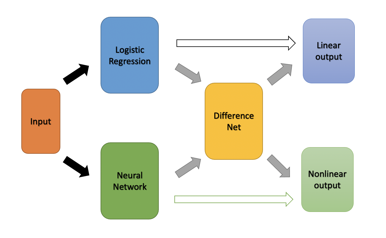
Figure 1: Two-stage Selective Learning

The output to the Difference Net can also be well approximated by the neural network by Theorem 2.2, as $1-|f-g|$ is continuous given $f$ and $g$ continuous. As a byproduct, the rejection rate, the percentage of samples with $z=0$, can also be learned by the Difference Net [31]. From Lemma 2.3, we notice that if $f$ and $g$ are smooth, the new solution becomes no longer differentiable. A smooth function could be fitted by a neural network with a higher order of approximation [25]. Therefore, in practice, more neurons are functioning in the Difference Net. Finally, we emphasize that the goal of the Difference Net is to provide an interpretation of neural networks, rather than to improve the accuracy.

2.2 Explanation of the neural network

It is important to note that different explanations [24] are required for diverse situations. The requirements of regulators and borrowers are well summarized in [1]. There are three types of explanations required in credit scoring, namely (i) global explanations, (ii) local instance-based explanations, and (iii) local feature-based explanations. Recently, sensitivity-based analysis has become increasingly popular in the interpretation of the results of neural networks [20, 19]. In this paper, we follow their analysis with slight modifications to accommodate the requirements of the credit scoring problem.

2.2.1 Global explanations

Global explanations describe how the classification model works in general, and they interpret the logic used in its prediction. In the credit rating industry, instead of relying on individual explanations of each instance, regulators, managers, and data professionals leverage global explanations to gain an overall understanding of the scoring model in order to ensure that the model is adequate and fair in its predictions.

In this paper, the relative importance of input features is used as the global explanation. We measure the relative importance of input features at a global level to understand what has been learned by the neural network during training, and we are mainly interested in variables that lead to rejection. The global importance of input features over the training dataset of the model is defined as follows:

$$\lambda_{j}=\frac{100}{C}\sqrt{\frac{1}{n}\sum_{i=1}^{n}\left(\frac{\partial f(\mathbf{x}_{i})}{\partial x^{j}}\right)^{2}},$$ (4)

where $n$ is the number of training samples in the case of independent observations. Here, $C$ is the normalization factor such that $\sum_{j=1}^{p}\lambda_{j}=100$, and $p$ is the number of input features. Global sensitivity is captured through partial derivatives, which are averaged across all training samples of the dataset. To avoid cancellation of positive and negative values, the square operation is used on top of the partial derivatives. This metric helps to construct a rank for features by their predictive power learned from the model. Indeed, a large value of this metric means that a large proportion of the neural network output sensitivity is explained by the considered variable. It also helps to filter out the insignificant features: a very small value of this metric means that the model outcome is almost insensitive to the feature.

Remark 2.4.

Categorical features are transformed into numerical variables for derivative computation. This is because neural networks are defined as differentiable and therefore can only handle continuous numerical features. Neural networks handle categorical features as continuous variables. With the transformation, previously described metrics can be naturally applied.

2.2.2 Local instance-based explanations

As opposed to global explanations, local explanations provide a local understanding of predictions at instance level. Loan officers prefer such explanations because they are interested in validating whether the predictions given by the model for a loan application is justified. Loan officers review the model’s prediction by looking at other similar loan applications with the same outcome to get an understanding of why a loan application has been denied compared to other loan applications that were previously accepted and then ended up defaulting [1]. This type of explanation is usually provided in the form of prototypes (i.e., categorizing the applications based on similarity).

Our Difference Net serves as the perfect tool for the local instance-based explanations. The logistic regression has provided good baseline accuracy for the dataset. While the neural network could further improve the logistic regression, the improvement is local. With the Difference Net, we are able to identify the local region where the neural network has significant improvements. With the localization, recurrent patterns can be found from data. Furthermore, the output from the logistic regression is combined with important features of samples to provide visualization. As a result, a typical explanation to use a neural network for a loan officer may resemble the following: “This person is rejected because his/her repayment in the last month has been delayed for 2 months, which is similar to A and B in the datasets. Although they have good credit scores calculated by the traditional method, A and B could not pay off.” Furthermore, we are able to provide the theoretical justification of the generalization error, which is discussed later.

2.2.3 Local feature-based explanations

Local feature-based explanations are concerned with how and why a specific prediction is made, at a local level. Such explanations are usually preferred by borrowers, as they are most interested in why their applications are denied. More importantly, this information can help them to improve their credit scores to obtain approval for loans in the future. If reasonable explanations are provided, they can work on their deficiencies to obtain better credit scores. Feature relevance scores or specific rules can be provided for these explanations. In terms of our selective learning, it is also beneficial to understand why certain samples are rejected by logistic regression.

A standard method to understand the local behaviors of a differentiable function is through the Taylor expansion. The Taylor series focuses on a small neighborhood of one sample of interest and provides a good approximation locally. Here, it can serve as a useful tool to capture the local relative importance of input features. In practice, a first-order Taylor expansion is usually sufficient for the analysis. Mathematically, for any input vector $\mathbf{x}$ close to $\mathbf{x}_{0}$, we have

$$f(\mathbf{x})-f(\mathbf{x}_{0})=(\mathbf{x}-\mathbf{x}_{0})^{T}\nabla f(\mathbf{x}_{0})+o(\|\mathbf{x}-\mathbf{x}_{0}\|)$$ (5)

for $\mathbf{x}\rightarrow\mathbf{x}_{0}$. The Taylor expansion shows that neural network output $f(\mathbf{x})$ can be well explained by its gradient locally. Then, for a sample $\mathbf{x}_{0}$ with input feature $j$, it is sufficient to look at its partial derivative as local importance:

$$\lambda^{j}_{0}=\frac{\partial f(\mathbf{x}_{0})}{\partial x^{j}}.$$ (6)

For categorical variables, we simply consider modifying the variable to the nearest value, i.e.,

$$\lambda^{j}_{0}=f(x_{1},\dots,x_{j}\pm 1,\dots,x_{p})-f(x_{1},\dots,x_{j},\dots,x_{p}).$$ (7)

If the difference is significant, then the feature is important locally. Intuitively, this informs us why such a data point belongs to the rejected set. These explanations can be provided by the neural network.

2.3 Concentration of measure results

We have designed a learning algorithm that can identify the rejection region of the logistic regression in the earlier section. As a byproduct, it is interesting to estimate the data rejection rate, i.e., the percentage of samples that are rejected. We provide the definition of the rejection rate.

Definition 2.5.

Assume that the training and test data follow from a universal underlying distribution with probability density function $\eta(\mathbf{x})$. Denote $\Omega_{d}$ and $\Omega_{nd}$ as the default and not default regions of the rejection region $\Omega$, respectively. The rejection rate is defined as the percentage of rejected data:

$$\gamma=\int_{\Omega_{d}}\eta(\mathbf{x})(1-p(\mathbf{x}))\ d\mathbf{x}+\int_{\Omega_{nd}}\eta(\mathbf{x})p(\mathbf{x})\ d\mathbf{x}.$$ (8)

We provide some theoretical justification of the data rejection rate. We require the rejection rate in the training set to serve as a natural and rigorous estimation of the intrinsic value for the population. This is called generalization, a key topic in machine learning. Generalization measures how accurately an algorithm can predict output values for unseen data. As an intrinsic value of an unknown dataset, the rejection rate provides us with important information about the non-linearity of the data and should be estimated accurately from outside of the sample. In this section, we study the generalization of the rejection rate. We provide a rigorous framework that uses the concentration of measures to estimate the rejection rate in testing.

For a sample $s$, if $\mathcal{I}$ is an indicator function and $\mathcal{I}_{s}$ indicates whether sample $s$ is rejected or not, then

$$\mathcal{I}_{s}=\begin{cases}1,&\text{with probability}\,\,\gamma\,;\\ 0,&\text{with probability}\,\,1-\gamma\,.\end{cases}$$ (9)

Let us say that $\mathcal{X}$ and $\mathcal{W}$ are the training and test sets. Denote by $n_{\mathcal{X}}$ and $n_{\mathcal{W}}$ the size of $\mathcal{X}$ and $\mathcal{W}$. Then, for $\{\mathbf{x}_{i}\}_{i=1}^{n_{\mathcal{X}}}\in\mathcal{X}$, we can write the training set rejection rate $\gamma_{\mathcal{X}}$ as $\gamma_{\mathcal{X}}=\frac{1}{n_{\mathcal{X}}}\sum_{i=1}^{n_{\mathcal{X}}}\mathcal{I}_{\mathbf{x}_{i}}$, where $\mathcal{I}_{\mathbf{x}_{i}}$ is the rejection indicator function. Similarly, for $\{\mathbf{w}_{i}\}_{i=1}^{n_{\mathcal{W}}}\in\mathcal{W}$, the test set rejection rate $\gamma_{\mathcal{W}}$ is $\gamma_{\mathcal{W}}=\frac{1}{n_{\mathcal{W}}}\sum_{i=1}^{n_{\mathcal{W}}}\mathcal{I}_{\mathbf{w}_{i}}$ where $\mathcal{I}_{\mathbf{w}_{i}}$ is the rejection indicator function. The following lemma indicates that the training rejection rate is close to the population rejection rate with high probability.

Lemma 2.6 (Concentration result between the training set and universal).

Assume that both $\mathcal{X}$ and $\mathcal{W}$ are from some universal distribution where each sample is rejected with probability $\gamma$. The inequality is satisfied for any positive $\epsilon_{1}$:

$$\mathcal{P}(\left\|\gamma_{\mathcal{X}}-\gamma\right\|\geq\epsilon_{1})\leq 2e^{-2n_{\mathcal{X}}\epsilon_{1}^{2}}\,.$$ (10)

Then, we need a concentration of measure results between the training and test set for generalization purposes.

Lemma 2.7 (Concentration between the training and test set).

Assume that both $\mathcal{X}$ and $\mathcal{W}$ are from some universal distribution where each sample is rejected with probability $\gamma$. Then, for any positive pair $(\epsilon_{1},\epsilon_{2})$, we have the following inequality:

$$\mathcal{P}(\|\gamma_{\mathcal{X}}-\gamma_{\mathcal{W}}\|\geq\epsilon_{1}+\epsilon_{2})\leq 2e^{-2n_{\mathcal{X}}\epsilon^{2}_{1}}+2e^{-2n_{\mathcal{W}}\epsilon^{2}_{2}}\,.$$ (11)

From the above lemmas, we can see that the rejection rate for the training set could be a good estimator of the rejection threshold of the population and test set.

3 Empirical results

While there have been many datasets used in the benchmark work [23], most of them are either not publicly available, lack variable names, or contain an insufficient number of samples which does not guarantee statistically significant results. In our study, we focus on two publicly available datasets, which have variable names that are easier to interpret, and also have enough samples such that our estimation of the rejection rate is statistical significance. In both datasets, the setup of neural networks and the optimization algorithms in backpropagation are the same. At the first learning stage, we train a neural network on the datasets and compare them with the conventional explainable logistic regression. The architecture is rather simple for credit scoring problems. Based on the model architecture optimization, we observe that one hidden layer of two units with the logistic activation function is sufficient. At the second learning stage, we construct a Difference Net and find that one hidden layer of five neurons is sufficient. The additional neurons are required as the output function becomes non-differentiable, as pointed out in Lemma 2.3. The backpropagation optimization is solved by the conjugate gradient method. We limit the total number of training epochs to 500 as the errors decay slowly.

We then study the model performance within each learning stage. The neural network is compared with the logistic regression within the first learning stage. As discussed in [23], there is no single perfect performance measurement for the credit scoring problem. In this study, three types of measurements are considered: (i) classification error — this tracks the percentage of the corrected prediction and is the most intuitive metric to evaluate the model fit; (ii) receiver operating characteristic curve (ROC) and area under the curve (AUC) — they provide a comprehensive evaluation of classification models. (iii) confusion matrix — in the credit scoring, it is important to correctly predict actual default cases, because false negatives may carry huge financial cost to banks. Although using other measurements that could potentially provide different insights into the model fit [23]. We believe classification error, ROC and AUC, and confusion matrix are sufficient since our primary concern of this study is model interpretation instead of model accuracy. We rely on the confusion matrix to further break down the default predictions by actual and predicted conditions. After comparing the global model performance at the first stage, we focus on analyzing performance of the Difference Net. As mentioned in Section 2.2.2, the Difference Net serves as a natural localized tool to find the rejection set which mostly contains predicted defaults by neural network. As AUC and ROC are not appropriate for evaluating highly skewed predictions, only the classification error is applicable to the rejected set for interpretation purpose. While the logistic regression might perform similarly to neural networks at the global level, there exists a significant difference at the local rejection region. Local evaluations could provide a more specific understanding of the model performance.

3.1 Taiwan data

3.1.1 Description of data

We first choose the Taiwan credit score dataset . The payment data in October 2015 was collected from an important bank (a cash and credit card issuer) in Taiwan and the targets were credit card holders of the bank. Among the total 30,000 observations, 6,639 (22.12$\%$) relate to the cardholders with default payments. This research employs a binary variable, default indicator, as the response variable. The dataset is randomly partitioned into the following sets: $75\%$ training set and $25\%$ test set. In addition, this dataset contains the following 23 variables as explanatory variables:

• $x_{1}$: Amount of the given credit (NT dollar): this includes both the individual consumer’s credit and his/her family (supplementary) credit.

• $x_{2}$: Gender (1 = male; 2 = female).

• $x_{3}$: Education (1 = graduate school; 2 = university; 3 = high school; 0,4,5,6 = others).

• $x_{4}$: Martial status (1 = married; 2 = single; 3 = divorce; 0 = others).

• $x_{5}$: Age (years).

• $x_{6}-x_{11}$: History of past payments. These variables track the past monthly payment records (from April to September, 2005) as follows: $x_{6}$ = repayment status in September, 2005; $x_{7}$= the repayment status in August, 2005; …; $x_{11}$ = repayment status in April, 2005. The measurement scale for the repayment status is: $-2$ = No consumption; $-1$ = Paid in full; 0=The use of revolving credit; 1=Payment delay for one month; 2 = Payment delay for two months; …; 8=Payment delay for eight months; 9 = Payment delay for nine months and above.

• $x_{12}-x_{17}$: Amount of bill statement (NT dollar). $x_{12}$ = Amount of bill statement in September, 2005; $x_{13}$ = Amount of bill statement in August, 2005; …; $x_{17}$ = Amount of bill statement in April, 2005.

• $x_{18}-x_{23}$: Amount of previous payment (NT dollar). $x_{18}$ = Amount paid in September, 2005; $x_{19}$ = Amount paid in August, 2005; $x_{23}$ = Amount paid in April, 2005.

• $y$: Client’s behavior; 0 = Not default; 1 = Default.

3.1.2 Results

At the first stage, we compare the neural network and the logistic regression. The classification test error is $18.2\%$ for the logistic regression and $17.7\%$ for the neural network. This result is consistent with the literature [32]. The result indicates that, overall, the neural network has a slight improvement over the logistic regression. This is not surprising as the datasets are imbalanced here given that most of the clients are creditable. The logistic regression has already provided a good approximation to identify the non-default cases and therefore is very popular in practice. In addition, the AUC is $71.1\%$ for the logistic regression and $73.1\%$ for the neural network. The comparison of the ROC curve for the two methods is plotted in Figure 2. The neural network has a consistent improvement over the logistic regression. Next, we look at confusion matrix for further analyses. The confusion matrix for the logistic regression is shown in Table 1. The confusion matrix for the neural network is given in Table 2. These matrices show that the neural network has captured more relevant default cases than logistic regression, which is measured by recall in machine learning. More specifically, the recall of the logistic regression is 24.9$\%$, whereas the neural network achieves a recall of 31.3$\%$. This is a significant improvement because a higher recall means more actual defaults are retrieved by the model. Overall, these results show that the neural network has outperformed logistic regression in terms of accuracy with a higher recall for this dataset, and it is worth exploring where these improvements are made.

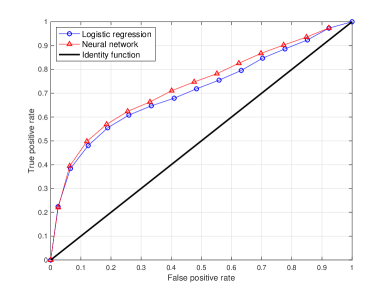
Figure 2: ROC curves of the logistic regression and the neural network of the Taiwan credit score dataset

$n=7500$	Predicted: Default	Predicted: Not default
Actual: Default	397	1198
Actual: Not default	168	5737

Table 1: Confusion matrix of the logistic regression for the Taiwan credit score dataset.

$n=7500$	Predicted: Default	Predicted: Not default
Actual: Default	500	1095
Actual: Not default	234	5671

Table 2: Confusion matrix of the neural network for the Taiwan credit score dataset.

At the second stage, we apply the Difference Net to the dataset. The classification test error is 1.6$\%$, indicating its predictive power. The percentage of predicted selected samples in the test set is 2.3$\%$, implying that, for most of the dataset, the logistic regression is sufficient. Therefore, we can have good confidence in the logistic regression in most cases. However, for approximately 2$\%$ - 3$\%$ of the dataset, the neural network strongly disagrees with the logistic regression. Special attention must be paid to this case. Conditioned on the rejected set, the classification test error is 63.8$\%$ for the logistic regression and 34.5$\%$ for the neural network. This indicates that, for the rejected set, the neural network has tremendously outperformed the logistic regression and hence should be adopted.

Further analyses are applied to the Difference Net. Among the rejected set, all samples are predicted as default by the neural network. At the global level, the Difference Net identifies samples where risks are underestimated by the logistic regression. 92.7$\%$ of rejected data has a payment delayed for two months in September 2015 (i.e., $x_{6}$ = 2). This pattern suggests that samples are rejected mainly due to the variable $x_{6}$, and further feature importance is no longer needed. For local feature-based explanations, we check samples with $x_{6}$ = 2 and find that the averaged difference of f(x) is 64.5$\%$ by modifying $x_{6}$ = 1, showing that $x_{6}$ plays an essential role in the rejected set. For local instance-based explanations, we combine the output from the logistic regression variable $x_{6}$. In Figure 3, we show the rejected set with respect to the logistic regression output and $x_{6}$. The result clearly indicates that, for overall lower-risk customers determined by logistic regression, if the $x_{6}$ = 2, then its risk is significantly underestimated, as pointed out by the neural network. This could provide a convincing explanation to local officers.

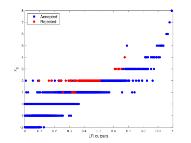
Figure 3: Predicted rejected samples for test data with respect to the logistic regression output and $x_{6}$ of the Taiwan credit score dataset.

3.2 Kaggle dataset—“Give me some credit”

3.2.1 Data description

We also test the Kaggle credit score dataset . For simplicity, data with missing variables are removed. The potential accuracy can certainly be improved with the appropriate consideration of samples with missing variables, but is not the primary concern of this paper. Among the total 120969 observations, 8,357 (6.95$\%$) relate to the cardholders with default payments. This indicates that the data are seriously imbalanced. Similarly, the dataset is randomly partitioned into $75\%$ training and $25\%$ test sets. The dataset contains 10 variables as explanatory variables:

• $x_{1}$: Total balance on credit cards and personal lines of credit except real estate and no installment debt such as car loans divided by the sum of credit limits (percentage).

• $x_{2}$: Age of borrower in years (integer).

• $x_{3}$: Number of times borrower has been 30 - 59 days past due but no worse in the last 2 years (integer).

• $x_{4}$: Monthly debt payments, alimony, living costs divided by monthly gross income (percentage).

• $x_{5}$: Monthly income (real).

• $x_{6}$: Number of open loans (installments such as car loan or mortgage) and lines of credit (e.g., credit cards) (integer).

• $x_{7}$: Number of times borrower has been 90 days or more past due (integer).

• $x_{8}$: Number of mortgage and real estate loans including home equity lines of credit (integer).

• $x_{9}$: Number of times borrower has been 60 - 89 days past due but no worse in the last 2 years (integer).

• $x_{10}$: Number of dependents in family, excluding themselves (spouse, children, etc.) (integer).

• $y$: Client’s behavior; 1 = Person experienced 90 days past due delinquency or worse.

3.2.2 Results

At the first stage, classification test errors are $7.1\%$ for the logistic regression and $6.8\%$ for the neural network. As the non-default cases cover approximately $7\%$ of the dataset, the classification errors are not informative. In addition, the AUC is $69.4\%$ for the logistic regression and $81.6\%$ for the neural network, indicating that the neural network outperforms the logistic regression. The comparison of the ROC curve for the two methods is given in Figure 4. These results are consistent with the results from Kaggle leaderboard. The confusion matrices for the logistic regression and neural network are provided in Table 3 and Table 4, respectively. Recall rates are 18.0$\%$ for the neural network compared to 3.1$\%$ for the logistic regression. These show that the neural network has a much better ability to capture the actual default cases. Thus, we are comfortable to conclude that the neural network has better predictive power in this dataset.

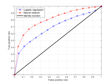
Figure 4: ROC curves of the logistic regression and the neural network of the Kaggle dataset.

$n=30067$	Predicted: Default	Predicted: Not default
Actual: Default	66	2072
Actual: Not default	50	27879

Table 3: Confusion matrix for the logistic regression of the Kaggle dataset.

$n=30067$	Predicted: Default	Predicted: Not default
Actual: Default	384	1754
Actual: Not default	287	27642

Table 4: Confusion matrix for the neural network of the Kaggle dataset.

At the second stage, we apply the Difference Net to the dataset. The Difference Net identifies $1.4\%$ of selected samples and only has $0.9\%$ classification test error. Among the rejected set, 99.7$\%$ of disagreement comes from predictions that the neural network predicts default, whereas the logistic regression predicts non-default. Among the rejected set, the neural network shows tremendous improvements over the logistic regression, with $40.4\%$ classification test error compared to $59.4\%$ for the logistic regression. The $19\%$ improvement suggests that neural network should be applied to the rejected set.

For global explanations, the feature importance of the Selected Net based on sensitivity analysis is given in Figure 5. Note that the variables $x_{7}$, $x_{9}$, and $x_{3}$ are the most important ones. Cumulatively, they explain $80\%$ of the variance. Therefore, we focus on these variables.

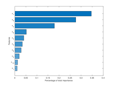
Figure 5: Global features importance of Difference Net of the Kaggle dataset.

For local instance-based explanations, we combine the output from the logistic regression variable. In Figure 6, we show the rejected set with respect to the logistic regression output and $x_{7},x_{9},x_{3}$ separately. The result clearly indicates that, for overall lower-risk customers determined by logistic regression, if these variables take large values, then the overall risk is significantly underestimated, as pointed out by the neural network. Therefore, recommendations to borrowers will be to reduce the number of past dues as represented by these variables. To understand why these variables fail to be captured by the logistic regression, we plot their logit functions in1 Figure 7. We observe diminishing marginal effects. Taking $x_{7}$ as an example, there will be a huge difference in the probability between cases that the payment is never past due once. However, for these past due cases, whether it is four or five times has little difference. This effect introduces non-linearity to the model and therefore cannot be explained by the logistic regression. Overall, qualitatively, we obtain results similar to the Taiwan dataset.

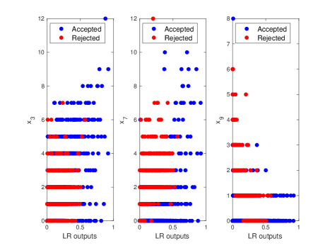
Figure 6: Predicted rejected samples for test data with respect to the logistic regression output and $x_{3},x_{7},x_{9}$ of the Kaggle dataset.

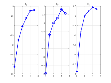
Figure 7: Non-linearities of logit functions of $x_{3},x_{7},x_{9}$ in the Kaggle dataset.

4 Conclusions

In this paper, we study the usage of the machine learning method in credit scoring. As introduced, some complicated non-linear machine learning methods have better predictive power; however, they are considered black-box structures without the good interpretability required by financial regulators. As a consequence, they have not been widely adopted in credit scoring. To resolve this issue, we introduce a neural network with the selective option to distinguish whether the datasets can be explained by the linear models or not. For the portion of the datasets that cannot explained by the linear model well, our learning model can feed the data into more complex machine learning methods. According to our model, we observe that, for most of the datasets, the logistic regression will be sufficient to achieve reasonably good accuracy; meanwhile, for some specific data portions, a shallow neural network model leads to much better accuracy without a significance sacrifice in interpretability. We show that machine learning does have better predictability than naive logistic regression. However, there is a compromise wherein the black-box machine learning method would lose its interpretability. Therefore, practitioners have been hesitant to adopt them. We propose a novel Selective Net, which can identify the data where the simple logistic regression fails. We show that, for most of the dataset, the logistic regression has been very useful. There is only a small amount of the dataset where the logistic regression would fail. Using the Difference Net, it is recommended that practitioners should still use the logistic regression for most cases, but they should switch to the neural network for specific regions. For future study, one possible direction is to generalize the selective learning framework to other complicated machine learning methods. Another potential direction of research would be to extend our method to other finance applications, including fraud detection and anti-money laundering. In these areas, interpretability is essential.

Supplementary

Proof of Lemma 2.3.

As the neural network has the true output $f(\mathbf{x})$, the probability of the difference between the logistic regression and the neural network is $|f(\mathbf{x})-g(\mathbf{x})|$. Therefore, the acceptance rate at $\mathbf{x}$ is $1-|f(\mathbf{x})-g(\mathbf{x})|$.

∎

Proof of Lemma  10.

From Hoeffding’s inequality, for any $\epsilon_{1}>0$,

$$\mathcal{P}\left(\left|\frac{1}{n_{\mathcal{X}}}\sum_{i=1}^{n_{\mathcal{X}}}\mathcal{I}_{\mathbf{x}_{i}}-\mathbb{E}\left[\frac{1}{n_{\mathcal{X}}}\sum_{i=1}^{n_{\mathcal{X}}}\mathcal{I}_{\mathbf{x}_{i}}\right]\right|\geq\epsilon_{1}\right)\leq 2e^{-2n_{\mathcal{X}}\epsilon_{1}^{2}}$$ (12)

where $\mathbb{E}\left[\frac{1}{n_{\mathcal{X}}}\sum_{i=1}^{n_{\mathcal{X}}}\mathcal{I}_{\mathbf{x}_{i}}\right]$ is equal to the universal rejected rate $\gamma$. From the definition of $\gamma_{\mathcal{X}}$ in the paper, (12) is equivalent to

$$\mathcal{P}(\left\|\gamma_{\mathcal{X}}-\gamma\right\|\geq\epsilon_{1})\leq 2e^{-2n_{\mathcal{X}}\epsilon_{1}^{2}}$$ (13)

This gives the concentration between training $\gamma_{\mathcal{X}}$ and universal $\gamma$.

∎

Proof of Lemma 11.

Same as the proof of Lemma 10, applying Hoeffding’s inequality on $\mathcal{W}$ and with the definition of $\gamma_{\mathcal{W}}$ in the paper; then, for any $\epsilon_{2}\geq 0$,

$$\mathcal{P}(\|\gamma-\gamma_{\mathcal{W}}\|\geq\epsilon_{2})\leq 2e^{-2n_{\mathcal{W}}\epsilon_{2}^{2}}$$ (14)

Apply the union bound on (13) and (14); then, with probability of more than $1-2e^{-2n_{\mathcal{X}}\epsilon_{1}^{2}}-2e^{-2n_{\mathcal{Z}}\epsilon_{2}^{2}}$, both of the following inequalities satisfy at the same time

$$\|\gamma_{\mathcal{X}}-\gamma\|<\epsilon_{1},$$

$$\|\gamma-\gamma_{\mathcal{W}}\|<\epsilon_{2}.$$

Use the triangle inequality, then

$$\|\gamma_{\mathcal{X}}-\gamma_{\mathcal{W}}\|\leq\|\gamma_{\mathcal{X}}-\gamma\|+\|\gamma-\gamma_{\mathcal{W}}\|<\epsilon_{1}+\epsilon_{2}$$

with probability more than $1-2e^{-2n_{\mathcal{X}}\epsilon_{1}^{2}}-2e^{-2n_{\mathcal{W}}\epsilon_{2}^{2}}$ as desired.

∎

References

- [1] Alejandro Barredo Arrietaa, Natalia Dıaz-Rodrıguezb, Javier Del Sera, Adrien Bennetotb, Siham Tabikg, Alberto Barbadoh, Salvador Garciag, Sergio Gil-Lopeza, Daniel Molinag, Richard Benjaminsh, et al. Explainable artificial intelligence (xai): concepts, taxonomies, opportunities and challenges toward responsible ai. arXiv preprint arXiv:1910.10045, 2019.
- [2] Bart Baesens, Tony Van Gestel, Stijn Viaene, Maria Stepanova, Johan Suykens, and Jan Vanthienen. Benchmarking state-of-the-art classification algorithms for credit scoring. Journal of the operational research society, 54(6):627–635, 2003.
- [3] Chaofan Chen, Kangcheng Lin, Cynthia Rudin, Yaron Shaposhnik, Sijia Wang, and Tong Wang. An interpretable model with globally consistent explanations for credit risk. arXiv preprint arXiv:1811.12615, 2018.
- [4] C. K. Chow. On optimal recognition error and reject tradeoff. In IEEE Transactions on Information Theory, 1970.
- [5] Corinna Cortes, Giulia DeSalvo, and Mehryar Mohri. Boosting with abstention. Advances in Neural Information Processing Systems, 2016.
- [6] George Cybenko. Approximation by superpositions of a sigmoidal function. Mathematics of control, signals and systems, 2(4):303–314, 1989.
- [7] Sanjeeb Dash, Oktay Günlük, and Dennis Wei. Boolean decision rules via column generation. arXiv preprint arXiv:1805.09901, 2018.
- [8] Elena Dumitrescu, Sullivan Hue, Christophe Hurlin, and Sessi Tokpavi. Machine learning for credit scoring: Improving logistic regression with non-linear decision-tree effects. European Journal of Operational Research, 297(3):1178–1192, 2022.
- [9] Steven Finlay. Multiple classifier architectures and their application to credit risk assessment. European Journal of Operational Research, 210(2):368–378, 2011.
- [10] Giorgio Fumera and Fabio Roli. Support vector machines with embedded reject option. Pattern recognition with support vector machines, 2002.
- [11] Yonatan Geifman and Ran El-Yaniv. Selective classification for deep neural networks. arXiv preprint arXiv:1705.08500, 2017.
- [12] Yonatan Geifman and Ran El-Yaniv. Selectivenet: A deep neural network with an integrated reject option. In International Conference on Machine Learning (ICML), 2019.
- [13] Oscar Gomez, Steffen Holter, Jun Yuan, and Enrico Bertini. Vice: visual counterfactual explanations for machine learning models. In Proceedings of the 25th International Conference on Intelligent User Interfaces, pages 531–535, 2020.
- [14] N Grennepois, MA Alvirescu, and M Bombail. Using random forest for credit risk models. Deloitte Risk Advisory, 2018.
- [15] David J Hand and William E Henley. Statistical classification methods in consumer credit scoring: a review. Journal of the Royal Statistical Society: Series A (Statistics in Society), 160(3):523–541, 1997.
- [16] Mohamad H Hassoun et al. Fundamentals of artificial neural networks. MIT press, 1995.
- [17] Martin E. Hellman. The nearest neighbor classification rule with a reject option. IEEE Transactions on Systems Science and Cybernetics, 6(3), 1970.
- [18] WE Henley et al. Construction of a k-nearest-neighbour credit-scoring system. IMA Journal of Management Mathematics, 8(4):305–321, 1997.
- [19] Enguerrand Horel and Kay Giesecke. Significance tests for neural networks. Journal of Machine Learning Research, 21(227):1–29, 2020.
- [20] Enguerrand Horel, Virgile Mison, Tao Xiong, Kay Giesecke, and Lidia Mangu. Sensitivity based neural networks explanations. arXiv preprint arXiv:1812.01029, 2018.
- [21] Kurt Hornik. Approximation capabilities of multilayer feedforward networks. Neural networks, 4(2):251–257, 1991.
- [22] Miroslav Kubat. Neural networks: a comprehensive foundation by simon haykin, macmillan, 1994, isbn 0-02-352781-7. The Knowledge Engineering Review, 13(4):409–412, 1999.
- [23] Stefan Lessmann, Bart Baesens, Hsin-Vonn Seow, and Lyn C Thomas. Benchmarking state-of-the-art classification algorithms for credit scoring: An update of research. European Journal of Operational Research, 247(1):124–136, 2015.
- [24] Joy Lu, Dokyun Lee, Tae Wan Kim, and David Danks. Good explanation for algorithmic transparency. Available at SSRN 3503603, 2019.
- [25] Hrushikesh N Mhaskar. Neural networks for optimal approximation of smooth and analytic functions. Neural computation, 8(1):164–177, 1996.
- [26] Giuseppe Paleologo, André Elisseeff, and Gianluca Antonini. Subagging for credit scoring models. European journal of operational research, 201(2):490–499, 2010.
- [27] Carla M. Santos-Pereira and Ana M. Pires. On optimal reject rules and roc curves. Pattern Recognition Letters, 26:943–952, 2005.
- [28] Venkat Srinivasan and Yong H Kim. Credit granting: A comparative analysis of classification procedures. The Journal of Finance, 42(3):665–681, 1987.
- [29] Paul Voigt and Axel Von dem Bussche. The eu general data protection regulation (gdpr). A Practical Guide, 1st Ed., Cham: Springer International Publishing, 10:3152676, 2017.
- [30] Jigang Xie, Zhengding Qiu, and Jie Wu. Bootstrap methods for reject rules of fisher lda. 18th International Conference on Pattern Recognition, pages 425–428, 2006.
- [31] Weicheng Ye, Dangxing Chen, and Ilqar Ramazanli. Learning algorithm in two-stage selective prediction. to appear in the Proceedings of 2022 Asia Conference of Algorithms, Computing, and Machine Learning, 2022.
- [32] I-Cheng Yeh and Che-hui Lien. The comparisons of data mining techniques for the predictive accuracy of probability of default of credit card clients. Expert Systems with Applications, 36(2):2473–2480, 2009.
- [33] Mumine B Yobas, Jonathan N Crook, and Peter Ross. Credit scoring using neural and evolutionary techniques. IMA Journal of Management Mathematics, 11(2):111–125, 2000.