Stochastic MPC with Realization-Adaptive Constraint Tightening

Abstract

This paper presents a stochastic model predictive controller (SMPC) for linear time-invariant systems in the presence of additive disturbances. The distribution of the disturbance is unknown and is assumed to have a bounded support. A sample-based strategy is used to compute sets of disturbance sequences necessary for robustifying the state chance constraints. These sets are constructed offline using samples of the disturbance extracted from its support. For online MPC implementation, we propose a novel reformulation strategy of the chance constraints, where the constraint tightening is computed by adjusting the offline computed sets based on the previously realized disturbances along the trajectory.

The proposed MPC is recursive feasible and can lower conservatism over existing SMPC approaches at the cost of higher offline computational time. Numerical simulations demonstrate the effectiveness of the proposed approach.

I Introduction

Stochastic model predictive control (SMPC) is a well established technique of MPC design for uncertain systems, where the state constraints are satisfied in probability with a user-specified bound [1]. This allows for violations of the constraints in order to improve the controller performance in closed-loop, where the performance is measured in terms of the closed-loop cost of trajectories. A literature review for SMPC is beyond the scope of this paper. For an overview, see a recent survey on SMPC [2], which includes references to [3, 4] (stochastic tube MPC with pre-stabilizing feedback control), [5, 6, 7] (affine disturbance feedback control), [8, 9, 10] (stochastic programming approach), etc.

With respect to reformulating the chance constraints, SMPC approaches can be broadly categorized into two groups: one group [4, 8, 11, 12] imposes the chance constraints for predicted states along the horizon, given the current state. Although easy to implement, these strategies cannot ensure recursive feasibility of the MPC problem in closed-loop. The second group [3, 13, 14] imposes the chance constraints on states along the horizon for all admissible predicted states at the previous step which are reachable from the current state under any disturbances. This guarantees recursive feasibility of the MPC problem with increased conservatism of the resulting controller [15].

In this paper, we propose a novel approach to design an affine state feedback policy as a solution to an SMPC problem with recursive feasibility guarantees. Compared to existing works [3], [14], this approach obtains a larger region of attraction (ROA) at the cost of increased offline computation. Precisely, we propose a Stochastic MPC schema which requires sets of disturbance sequences computed offline and its utilization on adaptive constraint tightening during online MPC implementation. In particular, in the offline phase, before the control implementation, we design sets of disturbance sequences that our controller needs to be robust against, in order to satisfy the imposed chance constraints. We propagate the additive uncertainty through system dynamics and find a bound of propagated uncertainty to tightly robustify the chance constraints. Similar to scenario based methods, such as [8, 9, 16], this offline step utilizes samples of disturbance. In the online phase, during control implementation, the imposed constraints in the MPC problem are determined by utilizing the aforementioned offline designed sets, and are adapted based on past disturbance realizations. This enables a realization-adaptive constraint tightening, which retains recursive feasibility, while lowering conservatism. Our key contributions can be summarized as:

• We propose an approach to construct subsets of the disturbance sequence support and use them to reformulate the chance constraints. These subsets are constructed offline before control implementation, using collected samples from the system trajectories.

• Utilizing the sets constructed offline, online during the receding horizon control implementation, we propose a novel reformulation of chance constraints with constraint tightening adjusted as a function of past disturbance realizations. At its core, the proposed reformulation can be interpreted as approximating the multivariate integral associated to state chance constraints at step $t+1$ by using a batch formulation involving all previous states and inputs from step $0$ to $t$. We show that this reformulated MPC problem is recursively feasible with a confidence level. As the number of offline samples increases, this reformulated MPC controller will satisfy the original chance constraints with higher confidence.

• We numerically compare our proposed stochastic MPC approach with the existing recursively feasible SMPC of [3]. We pick three different examples appeared in the literature. For these examples, the proposed approach obtains up to $35\%$ larger ROA and $6\%$ lower average closed-loop cost. The proposed method requires an additional offline computation time increasing linearly with the length of the task horizon. The approach [3] was chosen as a representative of the classes of approaches which impose the chance constraints on states along the horizon for all admissible predicted states at the previous step which are reachable from the current state under any disturbances. Other methods including [13, 14] belong to this class. Comparison to all other methods is outside the scope of this paper.

I-A Notation

For any vector $w$, $w_{l},w(l),w_{[l]}$ denote a random variable at time step $l$, the realization at time step $l$, a decision variable for an optimization at time step $l$, respectively. For any matrix $A$, $[A]_{i}$ denotes the $i^{\mathrm{th}}$ row vector.

II Problem Formulation

We consider an uncertain linear time-invariant (LTI) system:

$$x_{t+1}=Ax_{t}+Bu_{t}+w_{t},~{}x_{0}=x_{S},$$ (1)

where the system matrices $A\in\mathbb{R}^{n\times n}$ and $B\in\mathbb{R}^{n\times m}$ are known, $x_{t}\in\mathbb{R}^{n},u_{t}\in\mathbb{R}^{m},w_{t}\in\mathbb{R}^{n}$ denote the state, control input and disturbance at time $t$, respectively, and the additive disturbance $w_{t}$ is distributed according to an unknown probability distribution function (i.e., $w_{t}\sim f^{\mathrm{uk}}_{w}$), on a known bounded support $\mathbb{W}$. Our goal is to design a controller to regulate the system from the given initial state $x_{S}$, satisfying the state and input constraints given by:

$$\mathbb{P}(Hx_{t}\leq h)\geq 1-\bar{\alpha},~{}\forall t\in\{0,1,\dots,T\},$$ (2a)

$$H_{u}u_{t}\leq h_{u},~{}\forall t\in\{0,1,\dots,T-1\},$$ (2b)

where $H\in\mathbb{R}^{p\times n},H_{u}\in\mathbb{R}^{q\times m}$, $T\gg 0$ is the task duration, and $\bar{\alpha}\in(0,1)$ is a user specified upper bound on the probability of state constraint violation at each sample of the task duration. We apply Boole’s inequality to (2a) and consider the sufficient condition of the satisfaction of individual chance constraints as:

$$\mathbb{P}([H]_{i}x_{t}\leq h_{i})\geq 1-\frac{\bar{\alpha}}{p}=1-\alpha,~{}\forall i=\{1,\dots,p\},$$ (3)

where $h_{i}$ is the $i^{\mathrm{th}}$ element of $h$. Note that our choice of the same violation probability for each $i=\{1,2,\dots,p\}$ is only for the clarity of presentation in the subsequent sections.

II-A Finite Time Optimal Control Problem

We find feasible solutions to the following finite time optimal control problem:

$$\min_{u_{0},u_{1}(\cdot),\dots,u_{T-1}(\cdot)}{} \sum_{t=0}^{T-1}\ell(\bar{x}_{t},u_{t}(\bar{x}_{t}))+\ell_{F}(\bar{x}_{T})$$ (4)

s.t., $$x_{t+1}=Ax_{t}+Bu_{t}(x_{t})+w_{t},$$

$$\bar{x}_{t+1}=A\bar{x}_{t}+Bu_{t}(\bar{x}_{t}),$$

$$H_{u}u_{t}(x_{t})\leq h_{u},~{}\forall w_{t}\in\mathbb{W},$$

$$\mathbb{P}([H]_{i}x_{t+1}\leq h_{i})\geq 1-\alpha,$$

$$\forall i\in\{1,\dots,p\},$$

$$\forall t\in\{0,1,\dots,T-1\},$$

$$x_{0}=\bar{x}_{0}=x_{S},$$

where $\ell(\cdot,\cdot)$ denotes the stage cost, and $\ell_{F}(\cdot)$ denotes the final cost. Problem (4) is carried out over the space of feedback policies, $u_{t}(x_{t})$ which map the set of feasible states, subset of $\mathbb{R}^{n}$, to the set of feasible inputs, subset of $\mathbb{R}^{m}$. Pair $\{\bar{x}_{t},u_{t}(\bar{x}_{t})\}$ denotes the nominal state and the corresponding nominal input, respectively.

There are three main issues in solving (4), namely:

1. A large task horizon $T\gg 0$, can result in an unpractical computational burden while solving (4).

2. Optimizing over policies $\{u_{0},\dots,u_{T-1}(\cdot)\}$ is an infinite dimensional problem, and computationally intractable in general.

3. The distribution $f^{\mathrm{uk}}_{w}$ of the disturbance $w_{t}$ is unknown.

To address (I) and (II), we solve (4) in a receding horizon fashion, restricting ourselves to affine state feedback policies with a fixed stabilizing feedback gain $K$, i.e.,

$$u_{t}(x_{t})=Kx_{t}+v_{t},$$ (5)

where $v_{t}$ is the auxiliary input.

Assumption 1 (Strictly Stable)

Gain $K$ is chosen such that $A+BK$ is strictly stable.

Issue (III) is addressed by using a sample-based strategy. By sampling disturbance vectors propagated through system dynamics (1), we estimate disturbance sequence sets with the following property: if state constraints are satisfied robustly for all disturbance sequences in the sets, then the chance constraints (3) are satisfied for all $i=\{1,\dots,p\}$. Since our approach is sample-based, the former statement is true at the limit, i.e., with an infinite number of samples. These statements are formalized in the next section.

II-B Receding Horizon Reformulation

We consider the MPC reformulation of (4) in this section, with a horizon length of $N\ll T$. At time step $t$, $x(t)$ denotes the measured $x_{t}$ and let $x_{k|t}$ denote the predicted state for prediction step $k\in\{t,t+1,\dots,t+N-1\}$, obtained from $x(t)$ by applying the predicted input policies $\{u_{t|t},\dots,u_{k-1|t}(\cdot)\}$ to (1). In [3], recursive feasibility of the SMPC is guaranteed by imposing

$$\mathbb{P}([H]_{i}x_{k+1|t}\leq h_{i}|x_{k|t})\geq 1-\alpha~{}~{},~{}\forall i=\{1,\dots,p\},$$

which means that the chance constraints at time step $t$ for the predicted step $k+1$ are imposed for all the reachable states $x_{k|t}$ from the $x(t)$. The reachable set containing $x_{k|t}$ is computed by propagating $x(t)$ through the system dynamics under any admissible disturbances $\{w_{t},w_{t+1},\dots,w_{k-1}\}\in\mathbb{W}^{k-t}$ and the resulting optimal MPC policy. This condition is sufficient for the controller to satisfy (3) for the states in closed-loop with the MPC controller, but can be conservative, as pointed out in [15]. In order to reduce this conservatism and yet satisfy (3) in closed-loop with an MPC, we propose a new controller with offline computed disturbance sets and a realization-adaptive constraint tightening.

Approach Insight

To explain the proposed approach intuitively, we introduce a simple example in this section. We consider the system with given initial state $x_{0}$,

$$x_{t+1}=x_{t}+u_{t}+w_{t},$$ (6)

with 3 possible disturbances at every time step, i.e., $w_{t}\in\{-1,0,1\}$. Consider the problem of finding an input policy $u_{t}$ over two time steps (i.e., $t=0,1$) which satisfies the following constraints: $x_{2}\leq 1,x_{2}\geq-1$ with at least $\frac{2}{3}$ probability respectively, i.e., $\mathbb{P}(x_{2}\leq 1)\geq\frac{2}{3},\mathbb{P}(x_{2}\geq\text{-}1)\geq\frac{2}{3}$. Hard input constraints are $-1\leq u_{t}\leq 1$.

We first solve the above problem using the SMPC of [3]. As discussed before, it formulates the chance constraints for $x_{2}$ as follows:

$$\mathbb{P}(x_{2}\leq 1|x_{1})\geq\frac{2}{3},$$ (7a)

$$\mathbb{P}(x_{2}\geq-1|x_{1})\geq\frac{2}{3}.$$ (7b)

The feasible set $\mathcal{X}_{1}$ of all states $x_{1}$, where $x_{2}$ satisfies the constraints (7) when a suitable control policy $u_{1}$ is applied to the system (6), is obtained as follows. Each set of disturbances is obtained for tight robustification of (7a), (7b) respectively.

$$\exists u_{1},x_{1}\!+\!u_{1}\!+\!w_{1}\leq 1,\forall w_{1}\in\{0,-1\}\!\!\iff\!\!\exists u_{1},x_{1}\!+\!u_{1}\leq 1,$$

$$\exists u_{1},x_{1}\!+\!u_{1}\!+\!w_{1}\!\geq\!-1,\forall w_{1}\in\{0,1\}\!\!\iff\!\!\exists u_{1},x_{1}\!+\!u_{1}\!\geq\!-1,$$

$$\therefore-2\leq x_{1}\leq 2~{}(\because u_{1}\in[-1,1]),~{}~{}\mathcal{X}_{1}=[-2,2].$$ (8)

As discussed earlier, the approach of [3] imposes (7) for all reachable $x_{1}$ from $x_{0}$. Therefore, we find the 1-step robust controllable set $\mathcal{X}_{0}$ to $[-2,2]$ $\forall w_{0}$ (see [17, Chapter 10] for the definition) as follows:

$$\exists u_{0},-2\leq x_{0}+u_{0}+w_{0}\leq 2,~{}\forall w_{0}=\{-1,0,1\},$$

$$\iff \exists u_{0},-1\leq x_{0}\!+\!u_{0}\leq 1\therefore-2\leq x_{0}\leq 2,~{}\mathcal{X}_{0}=[-2,2].$$

Thus the feasible set of $x_{0}$, $\mathcal{X}_{0}^{\mathrm{Exist}}$ is $[-2,2]$ when the SMPC of [3] is utilized.

Consider now the proposed approach. This approach formulates the chance constraints by successively substituting $x_{t}+u_{t}+w_{t}$ for $x_{t+1}$ until $x_{0}$ appears. According to the following expression for $x_{2}\leq 1,x_{2}\geq-1$:

$$x_{2}=x_{0}+u_{0}+u_{1}+w_{0}+w_{1}\leq 1,$$ (9a)

$$x_{2}=x_{0}+u_{0}+u_{1}+w_{0}+w_{1}\geq-1,$$ (9b)

and the feasible set of $x_{0}$ is defined as a set of all states $x_{0}$, where $u_{0},u_{1}$ exist to robustly satisfy (9a), (9b) for 6 disturbance sequences (i.e., $(w_{0},w_{1})$) out of 9 possible disturbance sequences, respectively. The sets of these disturbance sequences are computed offline. Here the disturbance sequences are chosen to satisfy the $\frac{2}{3}$-probability tightly, i.e., (9a), (9b) hold for only the corresponding chosen sequences, not other remaining sequences. The sets $\hat{W}_{1}$ for (9a), $\hat{W}_{-1}$ for (9b) are obtained uniquely as:

$$\hat{W}_{1}\text{=}\{(w_{0},w_{1})|(\text{-}1,\text{-}1),(\text{-}1,0),(\text{-}1,1),(0,\text{-}1),(0,0),(1,\text{-}1)\},$$

$$\hat{W}_{-1}\text{=}\{(w_{0},w_{1})|(1,1),(1,0),(1,\text{-}1),(0,1),(0,0),(\text{-}1,1)\}.$$

We compute conditions for the controller to satisfy each of (9) robustly for any disturbance sequence in each set. For the first set $\hat{W}_{1}$, there exist $u_{0},u_{1}$ which satisfy (9a) robustly for $\forall(w_{0},w_{1})\in\hat{W}_{1}$ as below.

$$\exists(u_{0},u_{1}),x_{0}+u_{0}+u_{1}+w_{0}+w_{1}\leq 1~{}\forall(w_{0},w_{1})\in\hat{W}_{1},$$

$$\iff\exists(u_{0},u_{1}),~{}x_{0}+u_{0}+u_{1}\leq 1.$$

Likewise, $u_{0},u_{1}$ also should satisfy (9b) robustly for $\forall(w_{0},w_{1})\in\hat{W}_{-1}$ as below.

$$\exists(u_{0},u_{1}),x_{0}+u_{0}+u_{1}+w_{0}+w_{1}\geq\!-1~{}\forall(w_{0},w_{1})\!\in\!\hat{W}_{-1},$$

$$\iff\exists(u_{0},u_{1}),~{}x_{0}+u_{0}+u_{1}\geq-1.$$

Considering both constraints and the hard input constraints, we find the feasible set of $x_{0}$, $\mathcal{X}_{0}^{\mathrm{Prop}}$ as:

$$\exists(u_{0},u_{1}),-1\leq x_{0}+u_{0}+u_{1}\leq 1\iff-3\leq x_{0}\leq 3,$$

$$\therefore\mathcal{X}^{\mathrm{Prop}}_{0}=[-3,3].$$

In conclusion, when the proposed approach is applied, the final feasible set $\mathcal{X}_{0}^{\mathrm{Prop}}$, for which the constraints $\mathbb{P}(x_{2}\leq 1)\geq\frac{2}{3},\mathbb{P}(x_{2}\geq-1)\geq\frac{2}{3}$ are satisfied, is $[-3,3]$ which is a superset of $\mathcal{X}_{0}^{\mathrm{Exist}}$. Since $\mathcal{X}_{0}^{\mathrm{Prop}}$ contains $\mathcal{X}_{0}^{\mathrm{Exist}}$, our proposed approach can be less conservative intuitively while satisfying the chance constraint.

To demonstrate this difference between two approaches, Fig. 1 pictorially illustrates one scenario with $x_{0}=3$. The condition $x_{0}=3$ makes the SMPC problem of [3] infeasible, but makes the proposed SMPC problem feasible. In Fig. 1, each circle represents the state evolved through the system dynamics (6) without control inputs. Consider only the first constraint $\mathbb{P}(x_{2}\leq 1)\geq\frac{2}{3}$ here. MPC controllers try to make the colored circles satisfy the state constraints at $t=2$, by applying inputs over two steps. According to what we discussed earlier, the existing SMPC of [3] wants to satisfy the constraints for the blue circles in the left figure, and our proposed SMPC wants to satisfy the constraints for the red circles in the right figure. Our approach adaptively chooses the disturbances which the controller should be robust against depending on past realizations, while the existing SMPC always tries to satisfy the constraints robustly for the same two-thirds disturbances for any reachable states in the previous step. In Fig. 1 at $t=2$, the proposed SMPC tries to steer $[1,3]$ into $[-\infty,1]$ with $u_{0},u_{1}$ to satisfy $\mathbb{P}(x_{2}\leq 1)\geq\frac{2}{3}$, while the existing SMPC tries to steer $[1,4]$ into $[-\infty,1]$. Considering $-1\leq u_{t}\leq 1$, we can find $[1,4]$ cannot be steered into $[-\infty,1]$ within two steps, unlike $[1,3]$. Thus, $3$ is not in $\mathcal{X}_{0}^{\mathrm{Exist}}$ when applying the existing SMPC, whereas $3$ is in $\mathcal{X}_{0}^{\mathrm{Prop}}$ when applying the proposed SMPC.

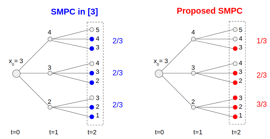
Figure 1: Tree diagram of a simple example scenario

Next we describe the proposed approach in details:

1. (Offline) Firstly we define a set of all possible disturbance sequences which contain $t$ disturbances up to time step $t$ for $t=0,\dots,T-1$ as $W^{\mathrm{seq}}_{0\rightarrow t}=\{[w_{0},\dots,w_{t-1}]|~{}w_{k}\in\mathbb{W},\forall k\}$. We find a subset $\hat{W}^{\mathrm{off},t}_{0\rightarrow t,i}$ of this set with the following property for all $i\in\{1,2,\dots,p\}$: If state constraints are satisfied robustly for all $[w_{0},\dots,w_{t-1}]$ in the subset, then the $i^{\mathrm{th}}$-chance constraint in (3) is satisfied tightly. The set consists of admissible disturbances from $0$ to $t-1$ satisfying: $\mathbb{P}([w_{0},\dots,w_{t-1}]\in\hat{W}^{\mathrm{off},t}_{0\rightarrow t,i})\geq 1-\alpha$. In other words, we should construct sets $\hat{W}^{\mathrm{off},t}_{0\rightarrow t,i}$ which guarantee the probability that a disturbance sequence from $0$ to $t-1$ belongs to the set, is at least $1-\alpha$. The construction of these sets is elaborated in Section III.

2. (Online) We design the MPC controller satisfying the state constraints robustly for any disturbance sequence in the offline computed sets. Next, let $0$ be the initial time of the control task, $t$ the current control time step and $k\geq t$ the time for which we are making predictions. Consider the realized disturbances along a trajectory until time step $t$ as $\mathbf{w}_{0\rightarrow t-1}=[w(0),\dots,w(t-1)]$. We construct a realization-adaptive set $\hat{W}^{\mathrm{on},k+1}_{t\rightarrow k+1,i}(\mathbf{w}_{0\rightarrow t-1})$ to compute the constraint tightening for prediction step $(k+1)$’s $i^{\mathrm{th}}$-state constraint $(\forall k\in\{t,\dots,t+N-1\},~{}\forall i\in\{1,\dots,p\})$ of the MPC problem solved at $t$. Such a set contains all the sequences $[w_{t},\cdots,w_{k}]$ which the MPC controller has to be robust against, in order to satisfy the $i^{\mathrm{th}}$-state constraint for any $[w_{0},\dots,w_{k}]\in\hat{W}^{\mathrm{off},k+1}_{0\rightarrow k+1,i}$. This set is constructed using $\hat{W}^{\mathrm{off},k+1}_{0\rightarrow k+1,i}$ discussed earlier and $\mathbf{w}_{0\rightarrow t-1}$. The construction of the sets $\hat{W}^{\mathrm{on},k+1}_{t\rightarrow k+1,i}(\mathbf{w}_{0\rightarrow t-1})$ is elaborated in Section IV. These disturbance realization-adaptive constraint tightenings allow the MPC problem not to impose excessively strict constraints, while satisfying (3) in closed-loop.

When both the offline and online methods are implemented, we obtain a MPC with lower conservatism over existing approaches and with recursive feasibility guarantees (in probability) at the cost of higher offline computation time. The robust MPC reformulation of (4) is given by:

$$\min_{v_{t|t},\cdots,v_{t+N-1|t}} \!\sum_{k=t}^{t+N-1}\!\!\ell(\bar{x}_{k|t},u_{k|t}(\bar{x}_{k|t}))+Q_{t+N\rightarrow T}(\bar{x}_{t+N|t})$$

$$\mathrm{s.t.,}~{}~{}~{}~{}~{}~{} x_{k+1|t}=Ax_{k|t}+Bu_{k|t}(x_{k|t})+w_{k|t},$$ (10a)

$$\bar{x}_{k+1|t}=A\bar{x}_{k|t}+Bu_{k|t}(\bar{x}_{k|t}),$$ (10b)

$$u_{k|t}(x_{k|t})=Kx_{k|t}+v_{k|t},$$ (10c)

$$x_{t|t}=\bar{x}_{t|t}=x(t),~{}~{}$$ (10d)

$$H_{u}u_{k|t}\leq h_{u},~{}\forall[w_{t|t},\dots,w_{k-1|t}]\in\mathbb{W}^{k-t},$$ (10e)

$$[H]_{i}x_{k+1|t}\leq h_{i},~{}\forall i\in\{1,\dots,p\},$$

$$\forall[w_{t|t},\dots,w_{k|t}]\in\hat{W}^{\mathrm{on},k+1}_{t\rightarrow k+1,i},$$ (10f)

$$\forall k=\{t,\dots,t+N-1\},$$

$$\bar{x}_{t+N|t}\in\mathcal{X}_{F}^{t},$$ (10g)

where $\mathcal{X}_{F}^{t}$ and $Q_{t+N\rightarrow T}(\cdot)$ denote the terminal set for the nominal state and the terminal cost for the prediction step $t+N$, respectively. The state $x(t)$ is the realized closed-loop state. Notice our control input should satisfy hard input constraints robustly for all disturbances in $\mathbb{W}$ in (10e), while state constraints are satisfied robustly for only disturbances in $\hat{W}^{\mathrm{on},k+1}_{t\rightarrow k+1,i}$. After solving (10), we apply

$$u_{t|t}^{\star}=Kx(t)+v^{\star}_{t|t}$$ (11)

to system (1) at time step $t$, with the first element $v^{\star}_{t|t}$ of the optimal solution sequence. We pick $\mathcal{X}_{F}^{t}$ so that a terminal policy $Kx$ can make the terminal state evolve while satisfying the state constraint (3) for all future time steps $(\geq t+N+1)$. The construction of this set is elaborated in Section IV.

III Offline Disturbance Sequence Sets

In this section, we first illustrate properties of the sets $\hat{W}^{\mathrm{off},t}_{0\rightarrow t,i}$ for $t\in\{0,1,\dots,T-1\},~{}i\in\{1,\dots,p\}$ and then show how we construct these offline with collected data. These sets will be computed by propagating the uncertainty using the system dynamics and then computing the constraint tightening which satisfies the chance constraints (3).

III-A Properties

Consider being at $x_{0}$. Under the control policy (5), the chance constraints on the very next state can be written as:

$$\mathbb{P}([H]_{i}x_{1}\leq h_{i})\geq 1-\alpha,$$ (12)

$$\iff \mathbb{P}([H]_{i}(Ax_{0}+Bu_{0}+w_{0})\leq h_{i})\geq 1-\alpha,$$

$$\iff \mathbb{P}([H]_{i}(A+BK)x_{0}+[H]_{i}Bv_{0}-h_{i}\leq-[H]_{i}w_{0})$$

$$\geq 1-\alpha,$$

for all $i\in\{1,2,\dots,p\}$. In (12), we can decouple the random variable terms and the decision variable terms. Once we find a $\gamma_{0,i}$ satisfying: For $w_{0}\in\mathbb{W}$ and $w_{0}\sim f^{\mathrm{uk}}_{w}$,

$$\mathbb{P}([H]_{i}w_{0}\leq\gamma_{0,i})\geq 1-\alpha,$$ (13)

then the set $\hat{W}^{\mathrm{off},1}_{0\rightarrow 1,i}$ can be defined as:

$$\hat{W}^{\mathrm{off},1}_{0\rightarrow 1,i}=\big{\{}w_{0}~{}\big{|}~{}[H]_{i}w_{0}\leq\gamma_{0,i},~{}w_{0}\in\mathbb{W}\big{\}}.$$ (14)

For the sake of brevity, we omit $w_{t}\in\mathbb{W}~{}\forall t$ in the disturbance sequence set definition in the rest of the paper. If our control policy robustly satisfies $[H]_{i}(A+BK)x_{0}+[H]_{i}Bv_{0}-h_{i}\leq-[H]_{i}w_{0}$, for all $w_{0}\in\hat{W}^{\mathrm{off},1}_{0\rightarrow 1,i}$, it also satisfies the chance constraint (12) for $w_{0}\in\mathbb{W}$ distributed according to $f^{\mathrm{uk}}_{w}$, unknown probability distribution. Ideally we pick the smallest $\gamma_{0,i}$ tightly satisfying (13). Then we construct the disturbance sequence set to tightly satisfy the $i^{\mathrm{th}}$-chance constraint for time step $1$.

Using the same approach, the $i^{\mathrm{th}}$-state constraint on a state $x_{t+1}$ formulated at time step $0$ can be expanded as:

$$\mathbb{P}([H]_{i}x_{t+1}\leq h_{i})\geq 1-\alpha,$$ (15)

$$\iff \mathbb{P}([H]_{i}(Ax_{t}+Bu_{t}+w_{t})\leq h_{i})\geq 1-\alpha,$$

$$\iff \mathbb{P}\Big{(}[H]_{i}(A+BK)^{t}x_{0}+\dots+[H]_{i}Bv_{t}-h_{i}\!\leq\!-([H]_{i}w_{t}+$$

$$[H]_{i}(A+BK)w_{t-1}+\dots+[H]_{i}(A+BK)^{t}w_{0})\Big{)}\!\geq\!1-\alpha.$$

From this expansion, we find the smallest $\gamma_{t,i}$ for each $t$ tightly satisfying:

$$\mathbb{P}\Big{(}[H]_{i}\big{(}\sum_{l=0}^{t}(A+BK)^{t-l}w_{l}\big{)}\leq\gamma_{t,i}\Big{)}\geq 1-\alpha.$$ (16)

Then, the set $\hat{W}^{\mathrm{off},t+1}_{0\rightarrow t+1,i}$ can be defined as:

$$\hat{W}^{\mathrm{off},t+1}_{0\rightarrow t+1,i}=$$

$$\big{\{}[w_{0},\dots,w_{t}]\big{|}[H]_{i}\big{(}\sum_{l=0}^{t}(A+BK)^{t-l}w_{l}\big{)}\leq\gamma_{t,i}\big{\}},$$ (17)

for each $i\in\{1,2,\dots,p\}$.

III-B Construction of $\gamma_{t,i}$ from Sampled Data

In this section we explain how to obtain $\gamma_{t,i}$, defining the sets $\hat{W}^{\mathrm{off},t+1}_{0\rightarrow t+1,i}$, from sampled data. Firstly, we consider a method to construct a set containing random variables with probability at least $1-\alpha$, using sampled data. Given a data set $D$ comprising samples of a random variable $d$, we construct $X(d)$ containing $d$ variables sorted by a given metric , from $0^{\mathrm{th}}$-percentile to $100(1-\alpha)^{\mathrm{th}}$-percentile, with confidence $1-\beta$ for $0<\beta\ll 1$, satisfying:

$$\mathbb{P}_{D}(\mathbb{P}(d\in X(d))\geq 1-\alpha))\geq 1-\beta,$$ (18)

using the method in [18]. $X(d)$ is chosen as a polytope and is computed as the convex hull of a part of samples, which contains from $0^{\mathrm{th}}$-percentile to $100(1-\alpha)^{\mathrm{th}}$-percentile samples sorted by the given metric. Also, as the number of samples increases, $\beta$ will decrease. For time step $t=0$, when the samples of $w_{0}$ realizations and the metric $[H]_{i}w_{0}$ are given, $X_{i}(w_{0})$ can be computed as explained in (18). $X_{i}(w_{0})$ is computed differently for each $i^{\mathrm{th}}$ constraint and we have $p$ different sets. Since $\mathbb{P}([H]_{i}w_{0}\leq\max\limits_{w_{[0]}\in X_{i}(w_{0})}[H]_{i}w_{[0]})\geq 1-\alpha$ with confidence $1-\beta$, we pick $\gamma_{0,i}$ as:

$$\gamma_{0,i}=\max_{w_{[0]}\in X_{i}(w_{0})}[H]_{i}w_{[0]},~{}\forall i\in\{1,2,\dots,p\},$$ (19)

where $w_{[0]}$ denotes the decision variable for optimization as described in Section I-A. For any time step $t>0$, $\gamma_{t,i}$ is also obtained in the same approach as follows. Define $y_{t}$ as:

$$y_{t}=w_{t}+(A+BK)w_{t-1}+\cdots+(A+BK)^{t}w_{0}.$$ (20)

That is, $y_{t}$ is the random variable which describes the summation of propagated disturbance terms from $0$ to $t$. With the realized samples of $y_{t}$, we construct $X_{i}(y_{t})$ using the aforementioned method, and find $\gamma_{t,i}$ as the solution to:

$$\gamma_{t,i}= \max_{y_{[t]}\in X_{i}(y_{t})}[H]_{i}y_{[t]}$$

$$= \max_{\begin{subarray}{c}[w_{[0]},\cdots,w_{[t]}]\end{subarray}}[H]_{i}\big{(}\sum_{l=0}^{t}(A+BK)^{t-l}w_{[l]}\big{)}$$

$$~{}~{}~{}~{}~{}~{}\text{s.t.,}~{}~{}y_{[t]}([w_{[0]},\cdots,w_{[t]}])\in X_{i}(y_{t})$$ (21)

Note $y_{t+1}$ can be computed as $y_{t+1}=w_{t+1}+(A+BK)y_{t}$.

Remark 1

With a large number of samples and a long task horizon $T$, computation of $\gamma_{t,i}$ can become cumbersome. In that case, we can opt for an efficient way to compute a conservative $\gamma_{t,i}$ for large values of $t$ as follows.

Given a $\gamma_{t,i}$, to compute the conservative $\gamma_{t+1,i}$ in an efficient manner, we use the following formula:

$$\gamma_{t+1,i}:=\max_{w\in\mathbb{W}}[H]_{i}(A+BK)^{t+1}w+\gamma_{t,i}.$$ (22)

If $\gamma_{t,i}$ satisfies (16), the $\gamma_{t+1,i}$ obtained from (22) also satisfies (16) for $t+1$, since $\mathbb{P}(w_{0}\in\{w_{0}|[H]_{i}(A+BK)^{t+1}w_{0}\leq\max\limits_{w\in\mathbb{W}}[H]_{i}(A+BK)^{t+1}w\})=1$ and $\mathbb{P}([w_{1},\dots,w_{t}]\in\{[w_{1},\dots,w_{t}]|[H]_{i}\big{(}\sum_{l=1}^{t}(A+BK)^{t-l}w_{l}\big{)}\leq\gamma_{t,i}\})\geq 1-\alpha$. This $\gamma_{t+1,i}$ is enough to satisfy (16) for $t+1$, although it is more conservative than the smallest $\gamma_{t+1,i}$ satisfying (16). Moreover, according to Assumption 1, we can find $\gamma_{t+1,i}\approx\gamma_{t,i}$ for sufficiently large $t$ because $(A+BK)^{t}w\approx 0$, so that we can set $\gamma_{t,i}$ as the fixed $\gamma_{\bar{t},i}$ for sufficiently large $t\geq\bar{t}$.

Note that when the disturbance distribution is known, we can find conservative $\gamma_{t,i}$ analytically (e.g., utilization of Chebyshev inequality in [3], etc.). This guarantees constraint satisfaction in closed-loop with confidence $1$. We approximately obtain $\gamma_{t,i}$ with our sampling method at the cost of constraint satisfaction with a confidence level less than $1$, so that we can tackle the unknown distribution of disturbance. With sufficient data, the confidence level will be $\sim 1$.

IV Realization Dependent Online Sets

Consider MPC problem (10) at current time step $t$ with MPC prediction step $k\in\{t,t+1,\dots,t+N-1\}$. We explain how to construct $\hat{W}^{\mathrm{on},k+1}_{t\rightarrow k+1,i}$, $\forall i\in\{1,\dots,p\}$ and $\mathcal{X}^{t}_{F}$ online. We obtain $\hat{W}^{\mathrm{on},k+1}_{t\rightarrow k+1,i}$ by utilizing past disturbance realizations and $\gamma_{k,i}$ which defines $\hat{W}^{\mathrm{off},k+1}_{0\rightarrow k+1,i}$, in order to satisfy the state constraints robustly for all disturbance sequences in $\hat{W}^{\mathrm{off},k+1}_{0\rightarrow k+1,i}$ in closed-loop. The terminal set for the nominal state, $\mathcal{X}^{t}_{F}$, is constructed specifically to ensure recursive feasibility of (10).

IV-A Construction of $\hat{W}^{\mathrm{on},k+1}_{t\rightarrow k+1,i}$ for $k\in\{t,\dots,t+N-1\}$

After obtaining the $\gamma_{k,i}$ using (III-B) and the past realized disturbances $\mathbf{w}_{0\rightarrow t-1}=[w(0),\dots,w(t-1)]$ at time step $t$, we can construct $\hat{W}^{\mathrm{on},k+1}_{t\rightarrow k+1,i}$ using $\gamma_{k,i}$ and $\mathbf{w}_{0\rightarrow t-1}$. $\hat{W}^{\mathrm{on},k+1}_{t\rightarrow k+1,i}$ is constructed as a set of $[w_{t|t},\dots,w_{k|t}]$ which satisfy the inequalities discussed next. For brief descriptions, we introduce the simplified terms for $k\in\{t,\dots,t+N-1\}$. Recall the notations from Section I-A.

$$a_{t,i}^{k}=[H]_{i}\big{(}\sum_{l=t}^{k}(A+BK)^{k-l}w_{l|t}\big{)},$$

$$M_{t,i}^{k}=\max\limits_{w_{[l]}\in\mathbb{W}~{}\forall l}[H]_{i}\big{(}\sum_{l=t}^{k}(A+BK)^{k-l}w_{[l]}\big{)},$$

$$m_{t,i}^{k}=\min\limits_{w_{[l]}\in\mathbb{W}~{}\forall l}[H]_{i}\big{(}\sum_{l=t}^{k}(A+BK)^{k-l}w_{[l]}\big{)},$$

$$b_{0,i}^{t-1,k}=[H]_{i}\big{(}\sum_{l=0}^{t-1}(A+BK)^{k-l}w(l)\big{)},$$

where $a_{t,i}^{k}$ denotes description of accumulated disturbances from $t$ to $k$, $M_{t,i}^{k}$ denotes the maximum of admissible accumulated disturbances from $t$ to $k$, $m_{t,i}^{k}$ denotes the minimum of admissible accumulated disturbances from $t$ to $k$, and $b_{0,i}^{t-1,k}$ denotes the accumulation of realized disturbances from $0$ to $t-1$ for $k$ prediction step. Then we define

$$\hat{W}^{\mathrm{on},k+1}_{t\rightarrow k+1,i}$$

$$=\Bigg{\{}[w_{t|t},\dots,w_{k|t}]\Bigg{|}\begin{cases}&\!\!\!\!a_{t,i}^{k}\leq M_{t,i}^{k},~{}~{}~{}~{}~{}~{}\text{if condition~{}(i)}\\ &\!\!\!\!\varnothing,~{}~{}~{}~{}~{}~{}~{}~{}~{}~{}~{}~{}~{}~{}~{}~{}~{}\text{if condition~{}(ii)}\\ &\!\!\!\!a_{t,i}^{k}\leq\gamma_{k,i}\!-\!b_{0,i}^{t-1,k},~{}\text{otherwise}\end{cases}\Bigg{\}}$$ (23)

for $i\in\{1,2,\dots,p\}$, where the conditions (i) and (ii) are:

1. $b_{0,i}^{t-1,k}\leq\gamma_{k,i}-M_{t,i}^{k}$,

2. ${b_{0,i}^{t-1,k}}>\gamma_{k,i}-m_{t,i}^{k}$.

The intuitive explanation behind the set description (IV-A) is presented next. The MPC controller is designed to satisfy the state constraints for all admissible disturbance sequences, which belong to $\hat{W}^{\mathrm{off},k+1}_{0\rightarrow k+1,i}$, with the past disturbance realizations up to time $t-1$.

• If the weighted sum of the disturbance sequence is small, resulting in condition (i) for $k$, then the controller tries to be robust against the entire $\mathbb{W}$ for future $k-t+1$ steps since all admissible disturbance sequences can belong to the offline computed set. So the set of disturbance sequences the controller would be robust against, will be decided as the largest set, equivalent to the first set description ($=\{[w_{t|t},\dots,w_{k|t}]\big{|}a_{t,i}^{k}\leq M_{t,i}^{k}\}$) in (IV-A).

• On the other hand, if the weighted sum of the disturbance sequence is very large, resulting in condition (ii) for $k$, then the accumulation of the disturbances from $0$ to $k$ cannot be less than or equal to $\gamma_{k}$ regardless of future disturbances from $t$ to $k$. In this case, the controller does not need to satisfy the state constraint at prediction step $k+1$ for any disturbance sequences. The user-specified upper bound $\alpha$ allows violation of constraints for these extreme disturbance realizations. These extreme disturbance realizations are already outside the offline disturbance sequence set defined by $\gamma_{k,i}$ in (III-A). It is equivalent to the second set description (i.e., empty) in (IV-A).

• If the weighted sum of the disturbance sequence is not extreme so that neither condition (i) nor condition (ii) holds, we can adjust the set of disturbance sequences depending on previous realizations as the third set description inequality ($=\{[w_{t|t},\dots,w_{k|t}]\big{|}a_{t,i}^{k}\leq\gamma_{k,i}-b_{0,i}^{t-1,k}\}$) in (IV-A).

Thus, the adjusted $\hat{W}^{\mathrm{on},k+1}_{t\rightarrow k+1,i}$ in (10f) can be computed online by (IV-A). The satisfaction of (3) is ensured with $1-\beta$ confidence due to the properties of chosen $\gamma$ parameters in Section III-A.

IV-B Construction of the terminal set $\mathcal{X}_{F}^{t}$

To keep recursive feasibility of (10), we define a terminal set $\mathcal{X}_{F}^{t}$ for prediction step $t+N$ at current time step $t$ as follows. If the nominal state enters this set at time $t+N$, the state chance constraints are satisfied at all future time steps for the states which evolve through the closed-loop system with a policy $u=Kx$. Define the terminal set $\mathcal{X}_{F}^{0}$ at time step $0$ first as:

$$\mathcal{X}_{F}^{0} =\Big{\{}x~{}\Big{|}~{}[H]_{i}A_{\mathrm{cl}}^{l+1}x\leq h_{i}-\gamma_{N+l,i},$$ (24)

$$~{}~{}~{}~{}~{}~{}\forall l=\{0,\dots,T-N-1\},~{}\forall i=\{1,\dots,p\}\Big{\}}$$

with $A_{\mathrm{cl}}=(A+BK)$. By recalling (15), we find that the nominal state $\bar{x}_{N}=\bar{x}_{N|0}$ in $\mathcal{X}_{F}^{0}$ evolves through the closed-loop system while satisfying all state chance constraints for all future time steps. The set $\mathcal{X}_{F}^{0}$ corresponds to the terminal set which is used in [3].

Considering $\bar{x}_{t+N|0}=\bar{x}_{t+N|t}-A_{\mathrm{cl}}^{N}\sum_{j=0}^{t-1}A_{\mathrm{cl}}^{t-1-j}w(j)$, we can construct the terminal set $\mathcal{X}_{F}^{t}$ for $\bar{x}_{t+N|t}$ from the set $\mathcal{X}_{F}^{0}$ as:

$$\mathcal{X}_{F}^{t} \!=\!\Big{\{}x\Big{|}[H]_{i}A_{\mathrm{cl}}^{l+1}x\!\leq\!h_{i}\!-\!\gamma_{N\!+t\!+l,i}\!+\![H]_{i}\!\sum_{j=0}^{t-1}A_{\mathrm{cl}}^{N\!+t\!+l\!-j}w(j),$$ (25)

$$~{}~{}~{}~{}~{}~{}\forall l=\{0,\dots,T-N-1-t\},~{}\forall i=\{1,\dots,p\}\Big{\}}$$

In practice, the set can be computed by only $\hat{N}$ inequalities ( $l=0,\dots,\hat{N}-1$), provided $\hat{N}$ is sufficiently large, according to [19]. We will show recursive feasibility of (10) in the next section’s Theorem 1 with the terminal set $\mathcal{X}_{F}^{t}$ in (25).

V Algorithm and Properties

Our algorithm is summarized in Algorithm 1.

0:  Sampled data $y_{t}~{}(t=0,1,\dots,T-1)$ in (20)

0:  Control Policy

Offline :

1:  Compute $\gamma_{t,i}$​​ $~{}\forall t\in\{0,1,\dots,T-1\},\forall i\in\{1,\dots,p\}$ which defines $\hat{W}^{\mathrm{off},t+1}_{0\rightarrow t+1,i}$ of (III-A), using (III-B) of Sec-

tion III-B.

Online :

2:  for $t=0$ to $T-N$ do

3:     Construct $\hat{W}^{\mathrm{on},k+1}_{t\rightarrow k+1,i}$ from $\gamma_{k,i}$, $\forall k\in\{t,\dots,t+N-1\},\forall i\in\{1,\dots,p\}$ and previous realizations $\mathbf{w}_{0\rightarrow t-1}$ using (IV-A)

4:     Solve MPC problem (10) at time $t$ with $\hat{W}^{\mathrm{on},k+1}_{t\rightarrow k+1,i}$

5:     Apply the first optimal policy $u^{\star}_{t|t}(x(t))$ to (1)

6:  end for

7:  For $t=\!T-\!N+1$ to $T-\!1$, apply the corresponding control policy from the optimal policy sequence $[u^{\star}_{T-\!N+1|T-\!N},\dots,u^{\star}_{T-\!1|T-\!N}]$ solved at time $T-\!N$.

Algorithm 1 SMPC with Realization-Adaptive Constraint Tightening

So far, we obtain the disturbance sequence sets for robust MPC policy in order to satisfy the chance constraints. Since the probability distribution of disturbance is unknown, we cannot obtain the smallest $\gamma_{t,i}~{}\forall t\in\{0,\dots,T-1\},~{}\forall i\in\{1,\dots,p\}$ satisfying (16) in analytical way. Practically, we should use the sampling method to obtain the approximate $\gamma_{k,i}$ in (III-B) with $1-\beta$ confidence, in order to construct the disturbance sequence sets. It implies that the chance constraint satisfaction in closed-loop can hold with $1-\beta$ probability. However, if we collect sufficiently large amount of samples, $\beta$ can be made negligibly small. Therefore, we consider the ideal case where $\beta$ can be regarded as zero and the smallest $\gamma_{t,i}~{}\forall t\in\{0,\dots,T-1\},~{}\forall i\in\{1,\dots,p\}$ satisfying (16) can be obtained. Next we show properties of Algorithm 1 when we assume $\beta=0$. With these disturbance sequence sets, we show that, for the state obtained from the system (1) in closed-loop with our MPC policy (11), there exists a MPC policy which satisfies (10f), (10g) recursively at every time step, while satisfying (3).

Theorem 1 (Recursive Feasibility)

Let (10) be feasible at time $t=0$, with the disturbance sequence sets $\hat{W}^{\mathrm{on},k+1}_{0\rightarrow k+1,i}~{}(k=0,\dots,N-1,~{}i=1,\dots,p)$ computed using Algorithm 1. Then, (10) remains feasible at all time steps $t\geq 0$ robustly for any admissible $x(t)$, if the state $x(t)$ is obtained by applying the closed-loop MPC control (11) to system (1).

Proof:

See Appendix. ∎

VI Numerical Simulations

In this section, we numerically compare the performance of the proposed SMPC in Algorithm 1 with the existing feasible SMPC approach in [3]. With Algorithm 1, we find MPC solutions to the optimal control problem (4) with $T=15,~{}N=6$ and we choose three sets of $A,B,H,h_{x},H_{u},h_{u}$, denoted with (E1), (E2), (E3), respectively in the Appendix. The cost function is quadratic, as shown in the Appendix, with penalty matrices $Q=Q_{F}=I_{2}$, $R=1$ and $x_{\mathrm{ref}}=[0,0]^{\top}$. We set the terminal cost of MPC as the LQR cost-to-go. We used the remaining parameters as: $\mathbb{W}=[-1,1]\times[-1,1],~{}\alpha=0.1,~{}K=K_{\mathrm{lqr}}$ (with the chosen $Q,R$). For the sampling method, we use $500$ disturbance samples. The optimization problems are formulated with YALMIP interface [20] in MATLAB, and we use Gurobi [21] to solve the associated quadratic programs for control synthesis.

VI-A Comparison of Approximate ROA

We compare the area of approximate ROA between two approaches for three examples respectively. To compute the approximate ROA, we choose the method in [22]. The approximate ROAs of the proposed MPC are about 7% - 35% larger in volume than that of the SMPC in [3]. They are described in the Fig. 2-4.

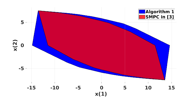
Figure 2: Comparison of approximate ROA with (E1)

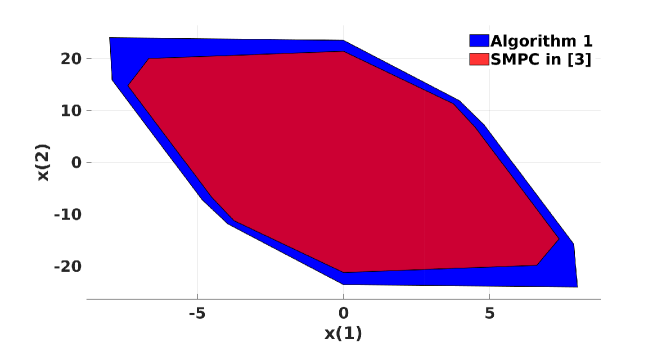
Figure 3: Comparison of approximate ROA with (E2)

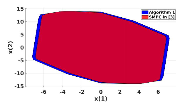
Figure 4: Comparison of approximate ROA with (E3)

VI-B Comparison of Performance

In this section, we focus on xmaple E2 and compare the average closed-loop cost of a realized trajectory over multiple realizations of the disturbance when the proposed approach and the SMPC approach in [3] is used We perform 10 trials and each trial contains different offline samples. In each trail, we get an average over 100 Monte-Carlo draws of the realized trajectory from the $x_{S}=[-5,19]^{\top}$. For comparison of performance when initial states change, several initial states $x_{S}$ are sampled in the ROA. Our proposed approach provides about $1\sim 6\%$ lower average closed-loop costs than [3], as shown in Table. I

	Algorithm 1	SMPC of [3]	Improvement(%)
Avg. cost	744.53	779.26	4.5
Best. cost	730.67	772.18	5.7

TABLE I: Closed-loop costs comparison.

In terms of computation time, our proposed approach requires almost the same online MPC computation time with the SMPC in [3] as you can see in Table. II. On the contrary, our proposed approach requires a long time to compute $\gamma_{t,i}~{}(t=0,\dots,T-1,~{}i=1,\dots,p)$ offline. The time complexity increases linearly with the length of task horizon. But, this procedure can be computed in advance and (22) can be used for large values of $t$ to reduce the computation time. Thus we can still use the proposed approach in practice.

	Offline	Algorithm 1	SMPC of [3]
Time(s)	2.2701	0.0976	0.0911

TABLE II: Computation times: Values are obtained with a ThinkPad P53, 2.60 GHz Intel Core i7-9850H, 16GB RAM.

VII Conclusions

We proposed a novel and efficient approach to design a stochastic MPC for constrained linear systems with an additive disturbance. In order to satisfy the imposed state chance constraints, the set of disturbance sequences that our controller needs to be robust against, were constructed offline from collected data. We also proposed a novel reformulation strategy of the chance constraints, where the constraint tightening is computed online by adjusting the offline computed sets based on the previously realized disturbances along the trajectory. The proposed SMPC was recursively feasible and had chance constraints satisfaction in closed-loop with a confidence level. With numerical simulations, we demonstrated that the proposed approach obtains a larger ROA and lower closed-loop costs in average over the existing feasible SMPC.

APPENDIX

VII-A Details of Parameters of Simulations

The cost function in (4) is defined as:

$$\ell(\bar{x}_{k},u_{k}(\bar{x}_{k}))$$

$$=(\bar{x}_{k}-x_{\mathrm{ref}})^{\top}Q(\bar{x}_{k}-x_{\mathrm{ref}})+u_{k}(\bar{x}_{k})^{\top}Ru_{k}(\bar{x}_{k}),$$

$$\ell_{F}(\bar{x}_{T})=(\bar{x}_{k}-x_{\mathrm{ref}})^{\top}Q_{F}(\bar{x}_{k}-x_{\mathrm{ref}}),$$

where $Q=Q_{F}=I$ and $R=1$.

1. Dynamics from Iterative SMPC [4]

   $$A=\begin{bmatrix}1.2&1.5\\ 0&1.3\end{bmatrix},B=\begin{bmatrix}0\\ 1\end{bmatrix},H=\begin{bmatrix}1&0\\ -1&0\\ 0&1\\ 0&-1\end{bmatrix},$$

   $$h=20\times\mathbf{1}_{4\times 1},H_{u}=\begin{bmatrix}1&-1\end{bmatrix}^{\top},h_{u}=\begin{bmatrix}6&6\end{bmatrix}^{\top}.$$

2. Dynamics from Strongly Feasible SMPC [14]

   $$A=\begin{bmatrix}1&0\\ 1&1\end{bmatrix},B=\begin{bmatrix}1\\ 2\end{bmatrix},H=\begin{bmatrix}1&0\\ -1&0\\ 0&1\\ 0&-1\end{bmatrix},$$

   $$h=20\times\mathbf{1}_{4\times 1},H_{u}=\begin{bmatrix}1&-1\end{bmatrix}^{\top},h_{u}=\begin{bmatrix}2&2\end{bmatrix}^{\top}.$$

3. Dynamics from Stochastic MPC [3]

   $$A=\begin{bmatrix}1.6&1.1\\ -0.7&1.2\end{bmatrix},B=\begin{bmatrix}1\\ 1\end{bmatrix},H=\begin{bmatrix}1&0\\ -1&0\\ 0&1\\ 0&-1\end{bmatrix},$$

   $$h=10\times\mathbf{1}_{4\times 1},H_{u}=\begin{bmatrix}1&-1\end{bmatrix}^{\top},h_{u}=\begin{bmatrix}10&10\end{bmatrix}^{\top}.$$

VII-B Proof of Theorem 1

Let (10) be feasible at time step $t$ and denote the corresponding optimal auxiliary input $v$ sequence as $[v_{t|t}^{\star},v^{\star}_{t+1|t},\cdots,v^{\star}_{t+N-1|t}]$, resulting in the corresponding optimal policies $[u_{t|t}^{\star},u^{\star}_{t+1|t}(\cdot),\cdots,u^{\star}_{t+N-1|t}(\cdot)]$ with (10c). Consider a candidate input $v$ sequence:

$$[v_{t+1|t}^{\star},\cdots,v^{\star}_{t+N-1|t},0],$$ (26)

at the next time $t+1$, resulting the corresponding optimal policies $[u_{t+1|t}^{\star}(\cdot),\dots,u^{\star}_{t+N-1|t}(\cdot),Kx_{t+N|t}]$. We need to show that sequence (26) is a feasible solution of problem (10) at time step $t+1$, when applying $u^{\star}_{t|t}$ to the system for any $w_{t}\in\mathbb{W}$. We will show the constraint satisfaction for any $i\in\{1,\dots,p\}$ and divide our proofs into two parts:

1. State constraint satisfaction of (10f)

2. Terminal constraint satisfaction of (10g)

1) State Constraint Satisfaction:

We will show satisfaction of (10f) for $k=t+N$ at time step $t+1$. With $A_{\mathrm{cl}}=A+BK$, the left-handed side in (10f) is written as:

$$~{}[H]_{i}x_{t+N+1|t+1}$$ (27)

$$= ~{}[H]_{i}\{A_{\mathrm{cl}}^{N}\big{(}A_{\mathrm{cl}}x_{t|t}+Bv_{t|t}^{\star}+w(t)\big{)}+$$

$$~{}\sum_{l=0}^{N-1}A_{\mathrm{cl}}^{N-1-l}(Bv_{t+1+l|t+1}+w_{t+1+l|t+1})\}$$

$$= ~{}[H]_{i}\{A_{\mathrm{cl}}^{N}\big{(}A_{\mathrm{cl}}\big{(}\bar{x}_{t|0}+\sum_{l=0}^{t-1}A_{\mathrm{cl}}^{t-1-l}w(l)\big{)}+Bv_{t|t}^{\star}+w(t)\big{)}$$

$$~{}+\sum_{l=0}^{N-1}A_{\mathrm{cl}}^{N-1-l}(Bv_{t+1+l|t+1}+w_{t+1+l|t+1})\}$$

$$= ~{}[H]_{i}A_{\mathrm{cl}}\bar{x}_{t+N|0}+b^{t,t+N}_{0,i}+a^{t+N}_{t+1,i}$$

We have $\bar{x}_{t+N|t}\in\mathcal{X}_{F}^{t}$ at the time $t$. Since we have $[H]_{i}A_{\mathrm{cl}}\bar{x}_{t+N|0}\leq h_{i}-\gamma_{t+N,i}$ by using $\bar{x}_{t+N|0}=\bar{x}_{t+N|t}-A_{\mathrm{cl}}^{N}\sum_{j=0}^{t-1}A_{\mathrm{cl}}^{t-1-j}w(j)$,

$$~{}[H]_{i}x_{t+N+1|t+1}$$ (28)

$$= ~{}[H]_{i}A_{\mathrm{cl}}\bar{x}_{t+N|0}+b^{t,t+N}_{0,i}+a^{t+N}_{t+1,i}$$

$$\leq ~{}h_{i}-\gamma_{t+N,i}+b^{t,t+N}_{0,i}+a^{t+N}_{t+1,i}$$

$$\leq ~{}h_{i}~{}\forall[w_{t+1|t+1},\dots,w_{t+N|t+1}]\in\hat{W}^{\mathrm{on},t+N+1}_{t+1\rightarrow t+N+1,i}$$

The last line holds when we consider the definition of $\hat{W}^{\mathrm{on},t+N+1}_{t+1\rightarrow t+N+1,i}$ in (IV-A). Therefore, (10f) for all $i\in\{1,\dots,p\}$ are satisfied for predicted step $k=t+N$ at time step $t+1$.

2) Terminal Constraint Satisfaction:

Now we prove that $\bar{x}_{t+N+1|t+1}$ satisfies the terminal constraint (10g) at $t+1$ when applying the candidate input sequence (26). Considering (26) as an input sequence at time step $t+1$ (i.e., $v_{t+N|t+1}=0$),

$$\bar{x}_{t+N+1|t+1}$$ (29)

$$= A_{\mathrm{cl}}^{N}\bar{x}_{t+1|t+1}+\sum_{l=0}^{N-1}A_{\mathrm{cl}}^{N-1-l}Bv_{t+1+l|t+1}$$

$$= A_{\mathrm{cl}}(A_{\mathrm{cl}}^{N}\bar{x}_{t|t}\!+\!A_{\mathrm{cl}}^{N\!-\!1}\!Bv_{t|t}^{\star}\!\!+\!\!\sum_{l=0}^{N-2}\!A_{\mathrm{cl}}^{N\!-\!2\!-\!l}Bv_{t\!+\!1\!+\!l|t\!+\!1})\!+\!A_{\mathrm{cl}}^{N}w(t)$$

$$= A_{\mathrm{cl}}\bar{x}_{t+N|t}+A_{\mathrm{cl}}^{N}w(t)$$

From (25), $\bar{x}_{t+N|t}\in X_{F}^{t}$ is written as:

$$~{}\forall l=\{0,\dots,T-N-1-t\},\forall i=\{1,\dots,p\},$$ (30)

$$[H]_{i}A_{\mathrm{cl}}^{l+1}\bar{x}_{t+N|t}\leq\!h_{i}-\!\gamma_{N+l+t,i}+[H]_{i}\sum_{j=0}^{t-1}A_{\mathrm{cl}}^{N+t+l-j}w(j)$$

$$\iff[H]_{i}A_{\mathrm{cl}}^{l}(A_{\mathrm{cl}}\bar{x}_{t+N|t}+A_{\mathrm{cl}}^{N}w(t))$$

$$~{}~{}~{}~{}~{}~{}~{}~{}\leq h_{i}-\gamma_{N+t+l,i}+[H]_{i}\sum_{j=0}^{t}A_{\mathrm{cl}}^{N+t+l-j}w(j)$$

Using (29) and (30),

$$[H]_{i}A_{\mathrm{cl}}^{l+1}\bar{x}_{t+N+1|t+1}$$ (31)

$$\leq h_{i}-\gamma_{N+t+1+l,i}+[H]_{i}\sum_{j=0}^{t}A_{\mathrm{cl}}^{N+t+1+l-j}w(j)$$

$$\therefore~{}\bar{x}_{t+N+1|t+1}\in\mathcal{X}_{F}^{t+1}$$

Therefore the terminal constraint (10g) is satisfied with the $\bar{x}_{t+N+1|t+1}$ obtained by applying the candidate sequence (26) to the system, at time step $t+1$.

From the state constraint satisfaction and the terminal constraint satisfaction, the problem (10) remains feasible at all time step $t\geq 0$. $\blacksquare$

References

• [1] M. Farina, L. Giulioni, and R. Scattolini, “Stochastic linear model predictive control with chance constraints–a review,” Journal of Process Control, vol. 44, pp. 53–67, 2016.
• [2] A. Mesbah, “Stochastic model predictive control: An overview and perspectives for future research,” IEEE Control Systems Magazine, vol. 36, no. 6, pp. 30–44, 2016.
• [3] M. Cannon, Q. Cheng, B. Kouvaritakis, and S. V. Raković, “Stochastic tube mpc with state estimation,” Automatica, vol. 48, no. 3, pp. 536–541, 2012.
• [4] U. Rosolia, X. Zhang, and F. Borrelli, “A stochastic mpc approach with application to iterative learning,” in 2018 IEEE Conference on Decision and Control (CDC).   IEEE, 2018, pp. 5152–5157.
• [5] B. Kouvaritakis, M. Cannon, and D. Muñoz-Carpintero, “Efficient prediction strategies for disturbance compensation in stochastic mpc,” International Journal of Systems Science, vol. 44, no. 7, pp. 1344–1353, 2013.
• [6] J. A. Paulson, S. Streif, and A. Mesbah, “Stability for receding-horizon stochastic model predictive control,” in 2015 American Control Conference (ACC).   IEEE, 2015, pp. 937–943.
• [7] J. A. Paulson, E. A. Buehler, R. D. Braatz, and A. Mesbah, “Stochastic model predictive control with joint chance constraints,” International Journal of Control, vol. 93, no. 1, pp. 126–139, 2020.
• [8] X. Zhang, K. Margellos, P. Goulart, and J. Lygeros, “Stochastic model predictive control using a combination of randomized and robust optimization,” in 52nd IEEE conference on decision and control.   IEEE, 2013, pp. 7740–7745.
• [9] G. C. Calafiore and L. Fagiano, “Stochastic model predictive control of lpv systems via scenario optimization,” Automatica, vol. 49, no. 6, pp. 1861–1866, 2013.
• [10] G. Schildbach, L. Fagiano, C. Frei, and M. Morari, “The scenario approach for stochastic model predictive control with bounds on closed-loop constraint violations,” Automatica, vol. 50, no. 12, pp. 3009–3018, 2014.
• [11] Y. Ma, J. Matuško, and F. Borrelli, “Stochastic model predictive control for building hvac systems: Complexity and conservatism,” IEEE Transactions on Control Systems Technology, vol. 23, no. 1, pp. 101–116, 2014.
• [12] T. A. N. Heirung, J. A. Paulson, J. O’Leary, and A. Mesbah, “Stochastic model predictive control—how does it work?” Computers & Chemical Engineering, vol. 114, pp. 158–170, 2018.
• [13] B. Kouvaritakis, M. Cannon, S. V. Raković, and Q. Cheng, “Explicit use of probabilistic distributions in linear predictive control,” Automatica, vol. 46, no. 10, pp. 1719–1724, 2010.
• [14] M. Korda, R. Gondhalekar, J. Cigler, and F. Oldewurtel, “Strongly feasible stochastic model predictive control,” in 2011 50th IEEE Conference on Decision and Control and European Control Conference.   IEEE, 2011, pp. 1245–1251.
• [15] M. Lorenzen, F. Dabbene, R. Tempo, and F. Allgöwer, “Constraint-tightening and stability in stochastic model predictive control,” IEEE Transactions on Automatic Control, vol. 62, no. 7, pp. 3165–3177, 2016.
• [16] M. C. Campi and S. Garatti, Introduction to the scenario approach.   SIAM, 2018.
• [17] F. Borrelli, A. Bemporad, and M. Morari, Predictive control for linear and hybrid systems.   Cambridge University Press, 2017.
• [18] L. J. Hong, Z. Huang, and H. Lam, “Approximating data-driven joint chance-constrained programs via uncertainty set construction,” in 2016 Winter Simulation Conference (WSC).   IEEE, 2016, pp. 389–400.
• [19] E. G. Gilbert and K. T. Tan, “Linear systems with state and control constraints: The theory and application of maximal output admissible sets,” IEEE Transactions on Automatic control, vol. 36, no. 9, pp. 1008–1020, 1991.
• [20] J. Lofberg, “Yalmip: A toolbox for modeling and optimization in matlab,” in 2004 IEEE international conference on robotics and automation (IEEE Cat. No. 04CH37508).   IEEE, 2004, pp. 284–289.
• [21] I. G. Optimization et al., “Gurobi optimizer reference manual, 2018,” URL http://www. gurobi. com, 2018.
• [22] M. Bujarbaruah, U. Rosolia, Y. R. Stürz, and F. Borrelli, “A simple robust MPC for linear systems with parametric and additive uncertainty,” in American Control Conference (ACC).   IEEE, 2021, pp. 2108–2113.