Multi-Tracer Groundwater Dating in Southern Oman using Bayesian Modelling
Abstract
In the scope of assessing aquifer systems in areas where freshwater is scarce, estimation of transit times is a vital step to quantify the effect of groundwater abstraction. Transit time distributions of different shapes, mean residence times and contributions are used to represent the hydrogeological conditions in aquifer systems and are typically inferred from measured tracer concentrations by inverse modelling. In this study, a multi-tracer sampling campaign was conducted in the Salalah Plain in Southern Oman including CFCs, SF6, 39Ar, 14C and 4He. Based on the data of three tracers, a two-component Dispersion Model (DMmix) and a nonparametric model with six age bins were assumed and evaluated using Bayesian statistics. In a Markov Chain Monte Carlo approach, the maximum likelihood parameter estimates and their uncertainties were determined. Model performance was assessed using Bayes Factor and Leave-One-Out cross validation. Both models suggest that the groundwater in the Salalah Plain is composed of a very young component below 30 years and a very old component beyond 1000 years, with the nonparametric model performing slightly better than the DMmix model. All wells except one exhibit reasonable goodness of fit. Our results support the relevance of Bayesian modelling in hydrology and the potential of nonparametric models for an adequate representation of aquifer dynamics.
Water Resources Research \addeditorauthor
Heidelberg University, Institute of Environmental Physics Heidelberg University, Kirchhoff-Institute for Physics Helmholtz Centre for Environmental Research, Leipzig Helmholtz Centre for Ocean Research, GEOMAR, Kiel Leipzig University of Applied Sciences (HTWK)
Viola Rädleviola.raedle@web.de
Groundwater in a semi-arid area was dated with multiple tracers including the first full-scale application of 39Ar with Argon Trap Trace Analysis
Bayesian Inference was applied for modelling the transit time distributions using a Markov-Chain Monte Carlo simulation
A Dispersion Model with two components and a nonparametric model with six age bins were applied, both suggesting a mixed groundwater of very old and very young origin
1 Introduction
According to the IPCC special report on Climate Change and Land [IPCC (\APACyear2019)], drylands (arid, semi-arid and dry sub-humid areas) currently cover about 46 % of the global land. Since the 1960s, dryland areas have expanded on average by about 1 % annually, due to desertification. In those regions, surface water is often rare and groundwater is the main source of freshwater supply for agriculture, industry, households and vegetation.
Under the influence of climate change, investigating groundwater systems in drylands is important in two aspects. First, about 3 billion people live in dryland regions where groundwater is often the main water source [van der Esch \BOthers. (\APACyear2017)]. Thus, groundwater management is most important and with that, a good understanding of groundwater dynamics, recharge and its response to water abstraction. Secondly, groundwater serves as a climate archive in which important information like infiltration temperatures and indicators of rainfall patterns are preserved. This makes groundwater analysis an important puzzle piece for paleoclimate reconstructions [Seltzer \BOthers. (\APACyear2021), Varsányi \BOthers. (\APACyear2011)].
The \change[author]here presented studystudy presented here investigates the groundwater system of the Salalah Plain in the South of Oman. While 82 % of the country is dominated by a hyper-arid sandy land desert [Al-Ajmi \BOthers. (\APACyear2013)], the Salalah region is categorized as semi-arid [Al-Ajmi (\APACyear2018)], mainly due to the annual Indian monsoon passing over the South of Oman. Still, water is scarce, as water consumption has drastically increased over the past decades driven by agricultural production [Shammas \BBA Jacks (\APACyear2007)]. This leads to a depletion of the local aquifers and saltwater intrusions from the ocean [Askri \BOthers. (\APACyear2016), Bear \BBA Cheng (\APACyear1999), Shammas \BBA Jacks (\APACyear2007)]. Furthermore, climate change driven alterations in rainfall patterns and sea level rise are likely to increase the stress on the existing freshwater reservoirs [Ahmed \BBA Choudri (\APACyear2012), Al-Habsi \BOthers. (\APACyear2014), Al-Sarmi \BOthers. (\APACyear2017), Gunawardhana \BBA Al-Rawas (\APACyear2016)]. To analyse and potentially mitigate the impacts of the water consumption on the aquifers, a profound understanding of the groundwater system of the Salalah Plain is crucial.
A very useful and well-proven tool to analyse groundwater dynamics is the concept of Transit Time Distributions (TTDs) [Kirchner \BOthers. (\APACyear2001), Małoszewski \BBA Zuber (\APACyear1982), McGuire \BBA McDonnell (\APACyear2006)]\remove[author](Sprenger et al., 2019). It assumes that the investigated water body represents a mixture of water with different ages, hence, travelling times between groundwater recharge and abstraction. The age distribution reflects certain properties of the groundwater system, like the ratio between advective and diffusive flow, the mean flow velocity or the travel distance from the point of recharge.
For groundwater age modelling, a specific type of TTD based on the hydrological setting is assumed and the free parameters of that TTD are constrained with tracer measurements. Typically, a variety of age tracers are applied, each covering a specific age range depending on their geochemical properties and atmospheric concentration. In this study, eight \add[author]dating tracers were used to investigate six monitoring and pumping wells. CFC-11, CFC-12, CFC-113 [Oster \BOthers. (\APACyear1996)]\change[author] and, SF6 [Busenberg \BBA Plummer (\APACyear2000), Newman \BOthers. (\APACyear2010)]\add[author]and 3H [I\BPBID. Clark \BBA Fritz (\APACyear1997\APACexlab\BCnt1)] were used to identify waters that infiltrated within the last 60 years, 39Ar was applied to cover the dating range between 100 and 1000 years [Loosli (\APACyear1983), Ritterbusch \BOthers. (\APACyear2014)] and 14C [I\BPBID. Clark \BBA Fritz (\APACyear1997\APACexlab\BCnt2), Torgersen \BOthers. (\APACyear2013\APACexlab\BCnt2), Vogel (\APACyear1968)] and 4He [Solomon (\APACyear2000)] were used for groundwater that recharged on the timescale of millennia. 39Ar is of special importance in this suite of tracers as it uniquely covers the intermediate age range. \citeARitterbusch2014 demonstrated that 39Ar analysis of groundwater samples by Atom Trap Trace Analysis (ATTA) [Lu \BOthers. (\APACyear2014)] is feasible. This study represents the first application of the 39Ar-ATTA or ArTTA technique for a complete set of groundwater samples and its integration in comprehensive age modelling of an aquifer system.
To derive a TTD from the measured tracer concentrations, modelling software of different complexity is available [Jurgens \BOthers. (\APACyear2012), Suckow (\APACyear2012)]. The modelling approach applied in the framework of this study is based on Bayesian statistics\change[author] and, using the tracers CFC-11, 39Ar and 14C. It incorporates the modelling of multiple water masses represented by analytical TTDs as well as shape-free age distributions which have been increasingly applied in the recent past [Massoudieh \BOthers. (\APACyear2014), McCallum \BOthers. (\APACyear2014)]. Furthermore, the model is capable of finding maximum likelihood estimates using a Markov-Chain Monte Carlo simulation and includes a comprehensive uncertainty analysis. To compare the models’ performance in terms of accuracy and simplicity, statistical key quantities to assess efficiency and predictive adequacy are computed. Evaluating the tracer data of the six wells with the described model allows for a \changesystematicalsystematic analysis of possible age distributions and with that, a profound interpretation of probable groundwater dynamics in the Salalah Plain.
2 Methods
2.1 Site description and sample processing
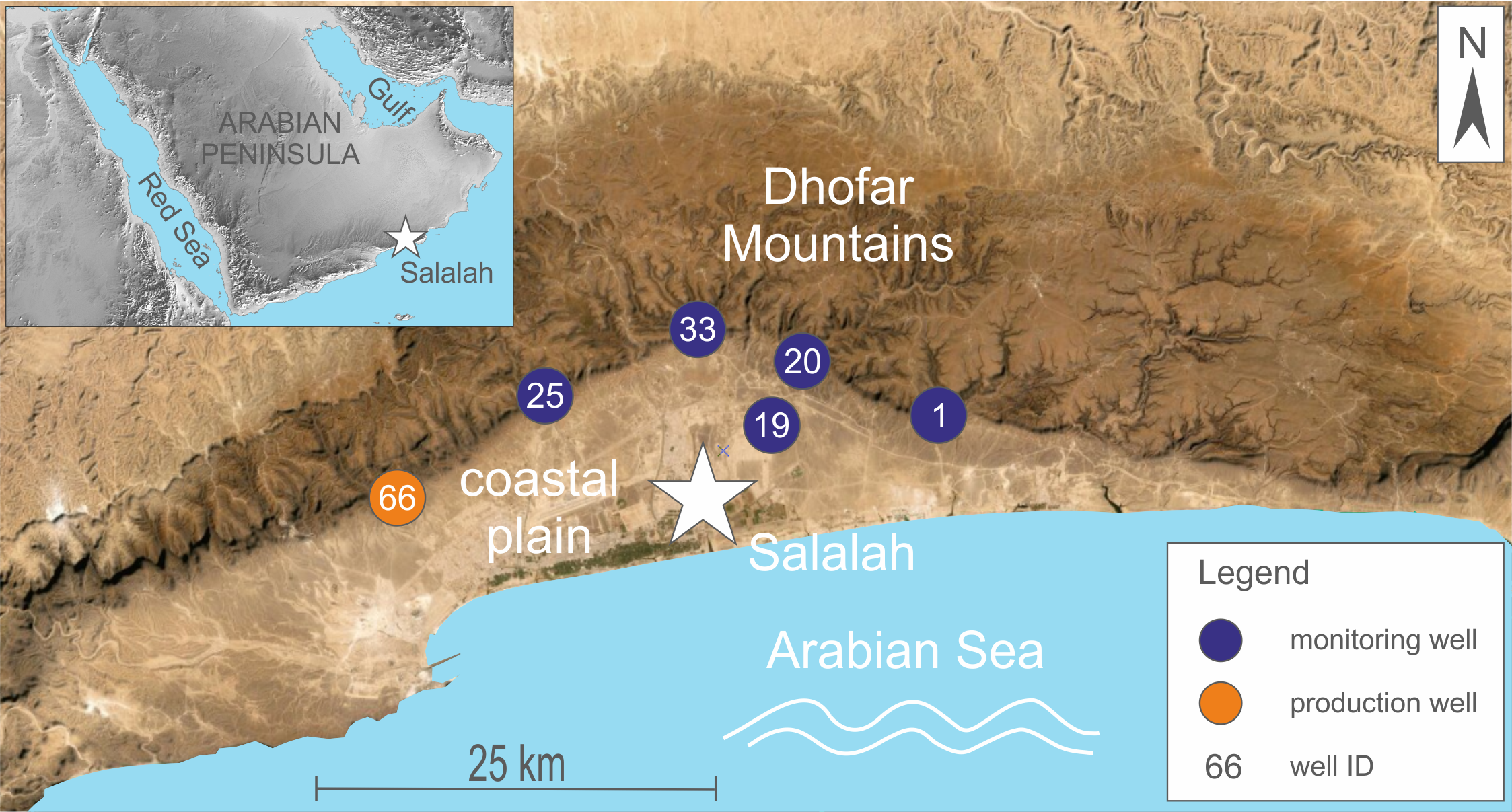
The Salalah Plain in Southern Oman forms a crescent shaped coastal enclave, with the Dhofar Mountain Range in the North and the Arabian Sea in the South. Being 60 km long and 15 km wide at its broadest point, the throughout flat plain is host of the City of Salalah with \change[author]overits around 300 000 \change[author]people the second largest city in the Sultanate of Omaninhabitants. The Dhofar Mountains are about 15 km wide in North-South direction. They rise steeply from the plain to elevations of around 900 meters in the center, separating the semi-arid south from the arid north. The area is affected by the Indian Summer Monsoon, with the mountain ridge as the Northern limit for the moisture. Precipitation is low on the plains (100 mm) and high in the mountains (up to 450 mm), with almost all precipitation during the monsoon between June and September [Shammas \BBA Jacks (\APACyear2007)]. The monsoon represents the most reliable water source of the study area [Bawain (\APACyear2012), I. Clark \BOthers. (\APACyear1987), Dames and Moore International (\APACyear1992)]. Additionally, occasional storm events can bring significantly more rainfall in a few days than in the rest of the year [Friesen \BOthers. (\APACyear2018), Müller \BOthers. (\APACyear2020)]. Those storms can cause vast flooding, leading to direct groundwater recharge in the plain. Karstified limestones form the aquifers in the mountains and in the coastal plain. The mountains are the main recharge area and groundwater reservoir, where the southward flow is higher in the center than in the East and West [GRC (\APACyear2004)]. The aquifer underlying the plain is the Fars formation, a shallow karstic limestone aquifer of tertiary origin with a saturated thickness of up to 70 meters. Groundwater users are the public water supply, agriculture and industry, with the main abstraction being in the central part of the plain, resulting in a deficit in the coastal water balance [Dames and Moore International (\APACyear1992), ICBA (\APACyear2012)].
In the study area, six groundwater \change[author]samples were taken, five from monitoring wells and one from a pumping wellwells were sampled, five monitoring wells and one pumping well (Figure 1). Before sampling the wells, the stagnant water was removed using a Grundfos MP1 submersible pump to prevent atmosphere-equilibrated water from contaminating the samples. \add[author]Temperature, pH, electrical conductivity (EC) and dissolved oxygen (Multi 3430, WTW, Weilheim, Germany) were measured on-site. The alkalinity was determined by titration with H2SO4 (AL-DT alkalinity test kit by HACH, Düsseldorf, Germany) and converted into bicarbonate concentrations. The wells were sampled for the analysis of ion chemistry, water stable isotopes, noble gases, carbon isotopes, tritium, 39Ar and transient trace gases. As this study focuses on groundwater dating, the geochemical data (water chemistry, stable isotopes, atmospheric noble gases) are not further discussed, except for their use in the interpretation of the tracers that can provide groundwater age information, i.e. radiogenic 4He, 14C, 39Ar, 3H, CFCs and SF6. For each well and dating tracer, duplicate samples were taken.
[author]The wells were sampled for analysis of 4He, 13C and 14C, 39Ar, 3H, CFCs and SF6. In addition, the temperature, pH, electric conductivity, titration and ion composition were measured to investigate the groundwater chemistry. For each well and tracer, duplicate samples were taken. \remove[author]The measured 3H concentrations were hardly significantly different from zero, therefore did not allow reliable differentiation between the wells (Table DS01). For the study region, it is very difficult to construct a reliable tritium input function for the entire relevant period including the bomb peak period, as no GNIP stations are nearby and even those from far away around the Indian ocean have only incomplete data [IAEA/WMO (\APACyear2021)]. \remove[author]For those reasons, tritium measurements were excluded from analysis.
Radiogenic 4He For noble gas sampling, crimped copper tubes, pinched off with stainless steel clamps for vacuum tight sealing, were used. The concentrations of stable noble gas isotopes were measured using mass spectrometry at the Institute of Environmental Physics, Heidelberg University. Using the software PANGA [Jung \BBA Aeschbach (\APACyear2018)], noble gas temperatures and helium components were modelled.
13C and 14C The carbon samples were taken using evacuated 100 mL glass bottles with a needle pinched through a rubber sealing. To avoid biological activity in the water sample, silver nitrate was added. At Heidelberg University, the carbon dioxide was extracted and reduced to carbon by graphitization. At the Curt Engelhorn Centre for Archeometry Mannheim, the 13C and 14C concentrations were measured using accelerator mass spectrometry (AMS).
39Ar For 39Ar sampling, an evacuated 12.2 L steel bottle was chosen as a suitable container, with a three-way brass adapter for flushing [Beyersdorfer (\APACyear2016), Ebser \BOthers. (\APACyear2018), Rädle (\APACyear2019)]. At Heidelberg University, the gas was extracted, the reactive gases were removed by gettering and the noble gases (about 2 mL) were stored in an Activated Charcoal Trap (ACT). The 39Ar concentration was measured using Argon Trap Trace Analysis (ArTTA), exploiting the high isotopic selectivity of the atom optical technique [Chen \BOthers. (\APACyear1999), Feng \BOthers. (\APACyear2019), Lu \BOthers. (\APACyear2014), Ritterbusch \BOthers. (\APACyear2014)]. Single 39Ar atoms are captured in a magneto-optical trap (MOT) and are identified by the emission of fluorescence photons. The count rate of the sample is compared to a reference, giving the concentration in percent modern argon (pmAr).
[author]3H: The samples were analyzed for tritium by means of Liquid Scintillation Counting after electrolytic enrichment. Concentrations were reported in Tritium Units (TU).
CFCs and SF6 The samples for Chlorofluorocarbons (CFCs) and Sulfur hexafluoride (SF6) analysis were stored in 500 mL stainless steel cylinders with ball valves. The concentrations were derived using gas chromatography (GC). Duplicate samples were taken of which the A samples were measured at Spurenstofflabor Wachenheim, Germany while the B samples were measured at Heidelberg University.
2.2 Transit time distributions
To characterize the dynamics of an aquifer system, dating tracers are applied to gather information on the time scales on which the subsurface flow takes place. The idealized groundwater age is defined as the time elapsed between the entering of water into the saturated zone and its sampling at a distance downstream within the groundwater system [Torgersen \BOthers. (\APACyear2013\APACexlab\BCnt1)]. However, one distinct value for the age (tracer age) only describes a purely advective regime with a point like recharge area. In reality, longitudinal and transverse dispersion leads to mixing along the flow path and between different flow paths, yielding a complex age spread denoted as transit time distribution (TTD) [Hall \BBA Plumb (\APACyear1994)].
The simplest TTD is the Piston-flow Model, where any kind of mixing is neglected (pure advection) and the screen of the well is infinitesimally small. Mathematically, this TTD is represented by a \add[author]Dirac delta distribution \change[author]with a probability of 1 foraround the mean age. In contrast, the Exponential Model is used for unconfined aquifers with a screen expanding from the bottom to the top [Vogel (\APACyear1968)]. All flow lines are considered, with \change[author]a weight of the input eventsthe contribution of recharge decreasing exponentially with age. The Dispersion Model is a solution for the advective-diffusive groundwater transport equation [Maloszewski (\APACyear1996)]. The two parameters are the mean residence time and the Péclet number , a measure of the relative importance of advection compared to the dispersion within a system [Waugh \BOthers. (\APACyear2003)]. As the Péclet number works as a shape parameter, the Dispersion Model approaches the Exponential Model for low Pe and the Piston-flow Model for large Pe. \add[author]Combinations of the above described TTD models or truncations of their age distributions are sometimes used for specific hydrogeologic situations [Jurgens \BOthers. (\APACyear2012)]. In addition to analytical age distributions\add[author] for a single groundwater component, mixing of several distinct water components from different reservoirs can occur. This is adopted by \add[author]binary mixing models combining two of the above models and weighting the individual TTDs by \change[author]theirthe mass contribution\add[author] of the components [Jurgens \BOthers. (\APACyear2012)]. Given that the dispersion model can describe flow conditions between no mixing (Piston-flow) and complete mixing (Exponential Model), we consider a binary mixing model that combines two independent Dispersion Models to be a flexible approach to approximate many realistic cases of groundwater systems.
If a water mixture cannot be described by analytical models, complex numerical methods can offer a broader range of possibilities [Broers \BOthers. (\APACyear2021), Cirpka \BOthers. (\APACyear2007), Troldborg \BOthers. (\APACyear2008), Visser \BOthers. (\APACyear2013)]. Those shape-free models, also called nonparametric models or age histograms, can help to identify the age contributions from a selected number of bins.
2.3 Multi-tracer modelling approach
2.3.1 Bayesian Inference and Maximum Likelihood
To address uncertainty in hydrological modelling, Bayesian methods have been widely applied \remove[author]in literature [Bates \BBA Campbell (\APACyear2001), Engeland \BOthers. (\APACyear2002), Liu \BBA Gupta (\APACyear2007), Vrugt \BOthers. (\APACyear2003)]. In Bayesian statistics, the probability \add[author] of a model given the data , also called the posterior, is computed by
| (1) |
with evidence , prior and likelihood [J\BPBIS. Clark (\APACyear2005)] whereas denotes the shape of the TTD as well as an attendant set of model parameters . The data are the measured tracer concentrations with measurement uncertainty.
As the exact form of the age distribution is not known, it can only be approximated by different presumed distribution functions that can be compared to one another. The prior contains the presumed distribution function and the parameter space given the constraints. In the present case, the mathematical models are a nonparametric model with six age bins and the mixture of two Dispersion Models with varying Péclet numbers\add[author] and mean ages (see Section 2.3.2). As no hydrological information is available before modelling, the prior is assumed uniform within the parameter constraints, resulting in a posterior proportional to the likelihood. The likelihood denotes the probability of observing a tracer configuration conditioned to a transit time distribution and a set of parameters . It is not normalized, and for numerical reasons the logarithm (log-likelihood) is used [Kolanoski (\APACyear2002)]:
| (2) |
with number of tracers n, representing the measured concentration of tracer j, and the tracer likelihood of measurement given the parameter set . Note that this is a modified realization to the standard definition found in literature as n does not denote the number of data points. Instead, each model evaluation is based on one data point in n-dimensional tracer space.
To calculate , the error of can be expressed in the form of a probability density [Yustres \BOthers. (\APACyear2012)]. The measurement uncertainty was used for all tracers except for 14C, where the uncertainty was enhanced due to the applied Vogel model with initial concentration of % [Vogel (\APACyear1968)]. The probability density was assumed to be normally distributed for all tracers except for 39Ar \change[author]which follows Poisson/Gaussian statisticsfor which a dedicated Bayesian error analysis accounting for the Poissonian atom counting statistics as well as other sources of error was conducted [Ebser (\APACyear2018), Feng \BOthers. (\APACyear2019)]. Hence, in lack of a parametrizable distribution, the numeric probability density distribution from the ArTTA measurements was used for 39Ar. The log-likelihood of tracer j is then determined by allocating , calculated by the mathematical model, in the probability density of the measurement data.
To calculate the evidence , a scalar normalization constant representing the probability of the data, it is necessary to integrate over the entire parameter space. However, the integral cannot always be evaluated, a problem known as intractable normalization. To approach this issue, the integral was approximated by summing over all parameter configurations.
An according approach is posed by the maximum likelihood estimate (MLE), a quantity independent of the evidence as the normalization does not change throughout the analysis [Cappé \BOthers. (\APACyear2002), Geyer \BBA Thompson (\APACyear1992)]. The corresponding parameter estimates represent the realization of a given model that comes closest to the measurements (conditioned to the limits of the parameter space).
As an additional, more intuitive quantity for the agreement of the calculated and the measured tracer concentrations, a likelihood score is calculated. Given as the likelihood of the estimates divided by the (model independent) likelihood of the exact measured tracer data , it serves as a relative measure and will be expressed in % throughout this paper.
2.3.2 Mathematical model
A mathematical model is deployed to calculate the tracer concentrations given the shape of the TTD and a parameter set . First, for the tracers involved in the modelling approach the concentration in water is derived for all (advective) ages , taking into account solubility and exponential decay. The solubility of CFC-11 in water is calculated according to \citeAWarner1985, using the Northern Hemispheric atmospheric input functions [NOAA (\APACyear2018)] and \change[author]the measuredmodelled input parameters. For 39Ar and 14C, radioactive decay is considered while taking into account a correction model for 14C (i.e. the Vogel model). Both are measured in relation to modern concentrations, with high values reflecting young water.
The two TTDs employed in the modelling approach are a Dispersion Model with two water masses (DMmix) and a nonparametric model. In a Dispersion Model, the age distribution function follows an inverse Gaussian regime:
| (3) |
with time in years before present, mean residence time (MRT) and Péclet number . Mixing two water masses with different and gives the (normalized) age distribution
| (4) |
with denoting the mixing ratio of the first water mass, yielding a parameter vector . The calculated concentration of tracer j is derived by
| (5) |
In case of presumed Péclet numbers, the parameter vector is reduced to , leaving three free parameters for the DMmix model.
For the nonparametric model, the concentration of tracer j (in water) in bin k (normalized by bin size) is computed by
| (6) |
for between the age limits { and } . The age limits can be chosen as required, depending on the desired resolution in the respective age regimes. With this, the concentration of tracer j is calculated:
| (7) |
with being the fraction of groundwater in bin k. Hence, for a nonparametric model with K = 6 bins\add[author] and given bin boundaries, there are five free parameters with fraction in the sixth bin .
2.3.3 Markov-Chain Monte Carlo methods
Finding the parameters of a TTD that best describes the groundwater system and can reproduce the observed tracer data is a typical inverse problem. This is addressed by modelling possible tracer results with different TTDs and parameter sets to project the (non-analytical) likelihood function. The Maximum Likelihood Estimate, meaning the best parameter set , is found by minimization of the weighted distance between the observed and the simulated values, leading to an optimization problem [Yustres \BOthers. (\APACyear2012)]. Yet, the presence of multiple local optima may interfere with simple optimization methods. A solution to this is provided by Markov-Chain Monte Carlo (MCMC) methods, \change[author]a Bayesianan approach for parameter estimation and uncertainty analysis [Zheng \BBA Han (\APACyear2016)]. As they can sample from virtually any posterior distribution without the need for an analytical expression, MCMC methods have been applied in multiple hydrological studies \add[author][Kuczera \BBA Parent (\APACyear1998), Laloy \BOthers. (\APACyear2013), Marshall \BOthers. (\APACyear2004), Massoudieh \BOthers. (\APACyear2012), Parno \BBA Marzouk (\APACyear2014), Smith \BBA Marshall (\APACyear2008), Vrugt \BOthers. (\APACyear2008), Zheng \BBA Han (\APACyear2016)]. In a Monte Carlo simulation, a multitude of parameter samples are generated based on the posterior distribution [Gamerman \BBA Lopes (\APACyear2006)]. To advance the parameter samples towards the optimum, a Markov chain is applied, meaning that the acceptance probability of a current state only depends on the immediately preceding state, not on the entire path [Sorensen \BBA Gianola (\APACyear2002)]. The procedure of choice is the broadly applicable Metropolis Hastings algorithm, generating new parameter sets depending on current one (Markov Chain) [Metropolis \BOthers. (\APACyear1953)], with a steady, normally distributed proposal density of width . First, a sample from the proposal density is drawn. In the next step, the likelihood of the proposed parameters is evaluated and compared to the previous one . Depending on the acceptance probability , the new parameters can be accepted (making the new original state, ) or rejected (starting from the same point again, ). Hence, the proposal density controls both the step size and the acceptance rate. To reach the target of the Metropolis-Hastings algorithm i.e. the maximum, it is desired to have a large step size with a simultaneous high acceptance probability [Gelman \BOthers. (\APACyear2013), Robert \BBA Casella (\APACyear2004)]. As the computational cost of MCMC is relatively high, it is necessary to adjust the algorithm by modifying the proposal distribution and the acceptance probability to improve the search efficiency. A two-step procedure was applied with an initial broad scan of the parameter space (large step size, tolerant acceptance probability) and a tuning around the maximum found in the first step (small step size, strict acceptance probability). \add[author]The MCMC algorithm was tested and tuned on synthetic data sets, as described in the Supporting Information (Text and Table S3).
2.3.4 Uncertainty of the fit results
To review the parameter estimates , it is crucial to infer their probability density functions. Using maximum likelihood, the uncertainty of the parameter estimates can only be calculated in particular cases. Generally, the whole covariance matrix is required [Kolanoski (\APACyear2002)]. For likelihood functions of known analytical forms, a Taylor series can be expanded around the maximum. As in this study, the likelihood does not correspond to known analytical distributions (i.e. the normal distribution), numerical methods are applied. To describe the likelihood regime, the moments of the function (mean, variance, skewness and kurtuosis) can be calculated. However, for a skewed distribution, the point of maximum likelihood does not correspond to the mean and due to constraints, the parameter space does not extend symmetrically to both sides. Therefore, this method is disregarded. Hence, the method of choice is the analysis of likelihood contours in parameter space. Those are hypersurfaces of constant likelihood forming an m-dimensional ellipsoid [Kolanoski (\APACyear2002)]. A confidence level of 68.27 % (corresponding to one standard deviation), is chosen as the partial integral of the likelihood within the error interval. The uncertainty of the parameter estimates is therefore derived as distance to the intersection of the parameter axes with the hypersurface.
2.3.5 Model selection techniques
In the context of model comparison, a vital step is the assessment of the model performance. Two common techniques are applied in the scope of this study, the Bayes factor and leave-one-out cross validation.
The Bayes factor corresponds to the goodness-of-fit across the entire parameter space and serves as a measure for the model performance [Jeffrey (\APACyear1961), Kass \BBA Raftery (\APACyear1995)]. Originally designed to compare the integrals of the likelihood given the prior density of two models, the Bayes Factor
| (8) |
will be expressed as the logarithm in this paper. Computation of Bayes factors has been found to be difficult [Ouarda \BBA El-Adlouni (\APACyear2011)], not least due to the required time investment. Incidentally, the averaging process in implicitly penalizes complexity as a vast parameter space will generally contain large stretches of poor fit quality [Vandekerckhove \BOthers. (\APACyear2015)].
Leave-one-out (LOO) cross validation is a cost intensive technique applicable for small data sets that is used to evaluate the predictive performance of a model more explicitly [Gelman \BOthers. (\APACyear2014), Gronau \BBA Wagenmakers (\APACyear2019), Stone (\APACyear1974)]. To validate how a model outcome generalizes to independent data, the observations are repeatedly partitioned into a training set and a test set. Consecutively, one observation i is excluded from modelling and the fit is carried out with the remaining data only. The ascertained posterior is employed for observation i as test data to assess predictive adequacy. In this study, each well corresponds to one data point in n-dimensional tracer space. Hence, instead of leaving out one of several data points, it is necessary to leave out one measurement . The resulting LOO posterior is computed using all tracers except for tracer i, denoted as , with the LOO log-likelihood
| (9) |
The total expected log likelihood for leave-one-out cross validation is deduced by the sum over the individual tracers i [Gelman \BOthers. (\APACyear2014), Gronau \BBA Wagenmakers (\APACyear2019)]:
| (10) |
with being the LOO posterior computed with tracer data and the likelihood of tracer . Bayesian computing includes sampling from the posterior over the whole parameter space, making the calculation very cost intensive. As a mesh grid, parameter step sizes of 1 y, 1000 y and 0.05 were chosen for MRT1, MRT2 and the ratio of the water masses, respectively. In practice, LOO-CV results can also be utilized to reveal the impact of the individual tracers on the parameter estimates, for a better understanding of the model.
In general, poor prediction capability may be caused by overparameterized models, a phenomenon denoted as overfitting, resulting in a trade-off between the prediction capability and model complexity. Quantities like the Akaike and the Bayesian Information Criterion punish complexity by adding a term including the number of free parameters to the likelihood function [Akaike (\APACyear1973), Schwarz (\APACyear1978)]. Furthermore, the Deviance Information Criterion [Draper (\APACyear1995)] is frequently applied in hydrological modelling approaches [Ju \BOthers. (\APACyear2020), Massoudieh \BOthers. (\APACyear2014), Reza Najafi \BBA Moradkhani (\APACyear2013)]. However, several prerequisites for those criteria, e.g. a normal distributed likelihood in parameter space [Spiegelhalter \BOthers. (\APACyear2002)], are not met by the here presented data, due to the mere fact that constraints set asymmetric boundaries.
3 Results
A summary of all measured tracer concentrations and field parameters is displayed in Table DS01 (Supporting Information). \add[author]The EC values range from 696 to 2270 S/cm. Wells 20, 25 and 33 at the foot of the Dhofar Mountains display fresh groundwater while more saline water is found in the East (well 1), West (well 66) and in the lower central plain (well 19).
Regional salinity differences have been described since the 1970s [Askri \BOthers. (\APACyear2016), Macumber \BOthers. (\APACyear1998), Shammas \BBA Jacks (\APACyear2007)] and led to the plain being divided into three zones, the ’Eastern Brackish Zone’, the ’Central Freshwater Zone’ and the ’Western Brackish Zone’. The origin of the salinization is not clear. It is assumed that, depending on the location and depth, different causes are responsible. Salt-bearing clays and marls occurring in the subsurface or the inflow of saline groundwater from deep aquifers triggered by reduced fresh water pressure in the pumped shallow aquifer come into question, but an oceanic origin (salt water intrusion due to groundwater extraction or previous flooding during times of higher sea-level) is also possible in some areas. On the other hand, the low EC values of wells 20, 25 and 33 at the foot of the mountains are easy to explain. They are located in the main inflow area from the mountains into the plain, where throughflow from the mountains is highest [Friesen \BOthers. (\APACyear2018)].
The measured \add[author]dating tracer concentrations are systematically evaluated by first examining their individual informative value. Subsequently, \change[author]the most robust set of tracersa subset of reliable tracers, as explained below, is used for modelling a Transit Time Distribution and parameters that represent the flow in the Salalah groundwater system best.
3.1 Tracers not involved in the modelling approach
While the groundwater samples were tested for a variety of\add[author] dating tracers, not all of them are suitable for a quantitative analysis. In Figure 2, unemployable tracers can be identified and excluded from analysis.
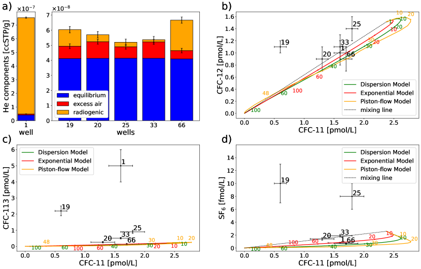
Radiogenic helium: The bar chart in Figure 2 a) shows the components of 4He as modelled with the software PANGA [Jung \BBA Aeschbach (\APACyear2018)]\change[author] using input parameters as described by Raedle (2019).. The standard (CE model) noble gas data evaluation yields moderate excess air contributions for an estimated infiltration altitude of 500 masl. The assumed conditions (altitude) and those derived from the noble gases (temperature, excess air) are used as constraints for the calculation of radiogenic 4He and equilibrium concentrations of CFCs and SF6. Otherwise, the stable noble gases only provide qualitative information on recharge conditions.
\change[author]Generally, more excess air is seen in wells located in the center of the plain. This may result from water table fluctuations (Aeschbach et al., 2002) between pre- and post-monsoon which are more pronounced in the central plain than in the East and West (Friesen et al., 2018). In addition, tThe central wells at the foot of the mountains (20, 25, 33) exhibit less 4Herad than wells downstream (19) or in the Western (66) plain\change[author], indicating younger water. which is attributed to the higher throughflow from the mountains and thus probably shorter residence times in this area. In contrast, well 1 in the Eastern plain exhibits 4Herad levels two orders of magnitude higher than the rest of the wells and is therefore plotted on a different scale. \add[author]The high helium value in this well is confirmed by a previous measurement and possibly due to geological factors. In West-East direction the geologic formations are more elevated in the East with the cretaceous formation outcropping at the surface in the area of well 1 [Platel \BOthers. (\APACyear1987), Platel \BOthers. (\APACyear1992)]. Other formations are thus flowed through and there is also a poorer connection to the mountain aquifer as the flow rates are lower compared to the central zone [Friesen \BOthers. (\APACyear2018)].
As the 4Herad accumulation rate \change[author]isand its spatial and temporal variability are unknown, those results only serve for qualitative analysis and will not be further employed in this paper.
[author]Tritium: The measured 3H concentrations are hardly significantly different from zero and vary only in a small range comparable to the measurement uncertainty, therefore do not allow reliable differentiation between the wells (Table DS01). The use of tritium as dating tracer in the study area is further hampered by the absence of any stations with precipitation data from the GNIP network [IAEA/WMO (\APACyear2021)] in the entire region. Even the few far away stations available around the Arabian Sea and Persian Gulf (Bahrain, Karachi, Mumbai) have only incomplete data. Thus, it is impossible to construct a reliable tritium input function for the entire relevant time including the bomb peak period and especially the last decades. The very few available data for the past 30 years suggest very low 3H contents of at most a few tritium units in precipitation at coastal stations around the Arabian Sea. The low measured 3H contents in some wells - if at all significant - can therefore not distinguish between remnants from the bomb peak period and fairly recent recharge. For those reasons, tritium measurements were excluded from analysis.
CFC-11 vs. CFC-12: In Figure 2 b), the measurements of CFC-12 are plotted against CFC-11. In addition, the possible relationships between the tracer concentrations for all mean residence times were modelled for the Piston-flow Model, the Exponential Model and the Dispersion Model (with Péclet number ) using the groundwater age modelling program Lumpy [Suckow (\APACyear2012)].\remove[author]For this purpose, input parameters similar to those for the 4He analysis were chosen. From visual interpretation, \change[author]the wells cannotnot all wells can be described by the applied models. While most wells show a high level of agreement with respect to their CFC-11 and CFC-12 data, the measurements for wells 19 and 25 are incompatible. \add[author]Potential unconsidered excess air would have a larger impact on CFC-12 than on CFC-11 due the lower solubility and could thus explain a deviation towards higher CFC-12. However, the moderate amounts of excess air derived from the noble gas measurements correspond to only small (few percent) effects for all CFCs. In contrast, the results at hand could arise from either a depletion of CFC-11 or a (small) contamination with CFC-12. While all CFCs are susceptible to contamination of anthropogenic origin [Darling \BOthers. (\APACyear2012), IAEA (\APACyear2006), Morris \BOthers. (\APACyear2006), Oster \BOthers. (\APACyear1996)], microbial degradation of CFC-11 in groundwater occurs only under anaerobic conditions [Khalil \BBA Rasmussen (\APACyear1989), Oster \BOthers. (\APACyear1996)]. However, all wells except well 19 show substantial concentrations of dissolved oxygen (5 to 6.5 mg/L, compare Table DS01) and can be considered aerobic. Only for well 19 with its lower oxygen level of 0.85 mg/L, an effect of anaerobic degradation appears possible. CFC-11 degradation is therefore only a plausible explanation for this single well, whereas indications for contamination are also present for CFC-113 and SF6, especially for wells 19 and 25 (see below). Moreover, for several wells the CFC-12 data are not in agreement with the tracers used for longer timescales, so a modelling approach appears only feasible using CFC-11. \remove[author]The results at hand can arise from either a depletion of CFC-11 or a (small) contamination with CFC-12. While all CFCs are susceptible to contamination of anthropogenic origin (IAEA, 2006; Morris et al., 2006; Oster et al., 1996; Darling et al., 2012), microbial degradation of CFC-11 in groundwater occurs only under anaerobic conditions (Oster et al., 1996; Khalil & Rasmussen, 1989). Although well 19 shows lower oxygen levels than the other wells (compare Table DS01), the conditions of all wells can be considered aerobic. An additional argument emphasizing the credibility of CFC-11 as a tracer is its higher solubility leading to a lower susceptibility to unconsidered excess air. An underestimation in excess air would hence produce a larger error in CFC-12 than in CFC-11. Moreover, for several wells the CFC-12 data are not in agreement with the tracers used for longer timescales, so a modelling approach is only feasible using CFC-11. Hence, CFC-12 data are disregarded for the multi-tracer modelling approach.
CFC-11 vs. CFC-113: In Figure 2 c), CFC-113 is plotted against CFC-11. For all wells except for well 66, the CFC-113 measurement data cannot be produced by any of the transit time distributions. This shows that most of the wells are contaminated with respect to CFC-113 and this tracer cannot be further applied for the model.
CFC-11 vs. SF6: In Figure 2 d), the CFC-11 and SF6 data can be seen. The SF6 concentrations of wells 19 and 25 are above atmospheric levels for any mean residence times, which can only result from a contamination or subsurface production in the central plain. Likewise, SF6 data will not be further used in this paper.
3.2 Tracers involved in the modelling approach
After considering the qualitative information of radiogenic 4He, CFC-12, CFC-113 and SF6, the\add[author] dating tracers remaining for a Bayesian modelling approach are 14C, 39Ar and CFC-11.\add[author]Of these tracers, 14C is the most complex to interpret as it is necessary to account for the dissolution of old carbon in groundwater. In literature, different correction methods for 14C are found\add[author], as reviewed by \citeAHan2016. A simple model relying entirely on chemical data, especially the alkalinity measurements shown in Table DS01 (Supporting Information), is the Tamers model. For near-neutral pH values as found in our samples (Table DS01), this model yields initial 14C activities close to 50 pmC, which would represent an overcorrection for all wells except for wells 19 and 20. Two widely used models are the the Pearson model, which relies solely on the C data of the samples (compare Figure S1 in the Supporting Information), and the Fontes-Garnier model, which combines chemical and isotopic data. Those models require C values of the end members soil air (modern component with 100 pmC) and calcite (old component with 0 pmC). For the soil air component, the mean (and its error) of four C values measured in the infiltration area were used, giving C ‰ [Al-Mashaikhi (\APACyear2011)]. For the carbonate end member, ‰ was assumed. However, with these assumptions both models fail due to overcorrection and produce negative apparent ages for all samples except well 19 (Pearson) and wells 19 and 66 (Fontes-Garnier). Overcorrection could be partly avoided by using more positive C values for the end members, but we consider that highly unlikely given that the assumed values are experimentally verified and already rather high in comparison to standard assumptions (e.g., -23 ‰ for Csoil and 0 ‰ for Ccalcite). Other models discussed by \citeAHan2016 correctly accounting for isotope exchange with soil CO2 under open conditions (Mook’s and Han & Plummer’s model) work for more samples, but still leave wells 20 and 25 overcorrected. We therefore assume that our measured C values are either not reliable or affected by additional processes that we cannot model. \remove[author]While the Pearson model relies on the 13C data of the samples (compare Figure S1 in the Supporting Information), the Fontes-Garnier and Tamers model are based on alkalinity measurements shown in Table DS01 (Supporting Information). However, those models fail due to overcorrection and produce negative apparent ages. Accordingly, the correction method of choice is the Vogel model with the concentration of modern 14C set to pmC due to the karstic aquifer environment in the Salalah Plain [Flint \BBA Rippon (\APACyear1986), Vogel (\APACyear1968)]. \add[author]This simple model with its uniform correction reflects the differences in the measured 14C activities, indicating substantially higher ages for wells 19 and 20 compared to the other samples. It may, however, lead to somewhat overestimated ages for these two wells by not accounting for their relatively high C values (compare Figure S1 in the Supporting Information).
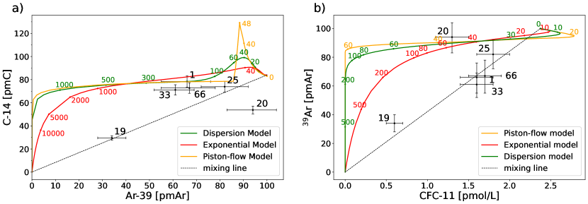
A tracer-tracer plot of 14C and 39Ar is shown in Figure 3 a), together with the calculated trajectories of different transit time distributions. \add[author]While the 39Ar input curve was assumed constant at 100 pmAr, the bomb peak from the Northern Atmospheric 14C input curve was considered. Only wells 1 and 25 seem to be consistent with the depicted models whereas all other wells clearly cannot be represented by a single water mass. However, the figure suggests the possibility of a mixed water with multiple components of different origin, whereas wells 19 and 20 may still pose difficulties. This observation is corroborated in Figure 3 b) where 39Ar and CFC-11 data are shown. For most wells, neither of the one-component age distributions can explain the measurements whereas with a mixing line of two or more water masses, this would be feasible.
3.3 Nonparametric model results
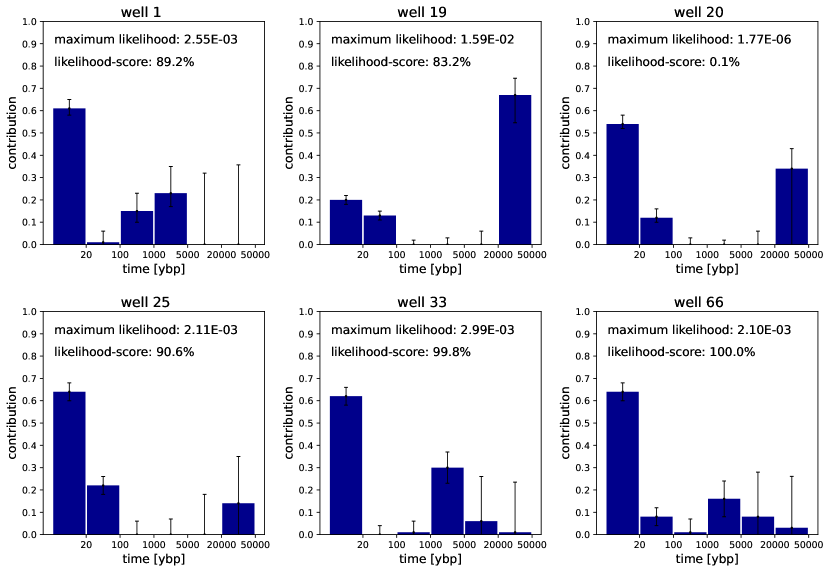
To allow for a transit time distribution with multiple maxima without imposing an analytic function, tracer concentrations were modeled using a nonparametric approach (as described in Section 2.3.2). Six age bins (resulting in five free parameters ) were selected with boundaries at 20, 100, 1000, 5000, 20000 and 50000 years, implying a constant age contribution within each bin k. Using a Markov-Chain Monte Carlo simulation with 20000 iterations, the best age distribution and the associated maximum likelihood were found. As start parameters, equal groundwater fractions in each bin were chosen. As can be seen in Figure 4, almost all wells show reasonable likelihoods, stating that the measured tracer concentrations may be produced by the displayed age histograms. The reason for the inadequate modelling likelihood of well 20 are the incompatible 14C and 39Ar measurements (compare Figure 3). The distributions among the age bins show two distinct age clusters: one very young component below 20 years of strong contribution and one old component of varying ages. While for well 66 many bins contribute with small shares, the other wells exhibit a gap between the young and the old cluster. High contributions above 20000 years before present are only found in wells 19 and 20. \add[author]Those results are visualized as cumulative age distributions in Figure S3 (Supporting Information).
3.4 DMmix model results
Based on the results of the nonparametric model, an analytical model can be designed to find the best representation of the hydrological system. Due to the clustering in very young and very old water, a two-component Dispersion Model (DMmix) with unknown Péclet numbers, mean residence times and unknown mixing ratio of the young contribution is chosen for the further analysis. As those parameters involve large parameter spaces and the analytical model brings along a high computation intensity, it is not possible to model all parameters at once. Instead, a set of Péclet numbers is preselected\add[author] (), reducing the number of free parameters from five to three. \add[author]A more thorough analysis of the Péclet space is described in the Supporting Information (Text S4 and Figure S4). Hence, only\remove[author] Subsequently, MRT1, MRT2 and the mixing ratio \add[author] of water mass 1 \add[author](the younger one) are optimized whereas not only the parameter estimates, but also the likelihood in parameter space is taken into account.
[author] Constraining the flow regime for DMmix
For each water mass, five different Peclet numbers are tested (5, 10, 100, 1000 and 10000). While low Peclet numbers indicate a regime where the Dispersion Model approaches the Exponential Model, high numbers suggesting an advective regime show a tendency towards a Piston-flow. For each of the 25 Peclet combinations, the highest achievable likelihood is calculated. For the Markov-Chain Monte Carlo simulation, a two step approach with a broad sampling in the whole parameter space (10000 iterations) and a more precise, more stringent scanning around the maximum (20000 iterations) are employed. FIGURE 5 The results are depicted in Figure 5. For a more intuitive visualization, the achievable likelihood given the measurement uncertainties (complying with the measured tracer concentrations) is applied as a normalization constant representing 100% likelihood. As mentioned in the methods section, the resulting quantity of the relative likelihood is denoted as likelihood score, indicated by the color scale. As the respective fit parameters (mean residence times and mixing ratio) are not of interest at this point, they are not displayed in the plot. For wells 1, 33 and 66, all Peclet combinations yield likelihoods above 99 % with no perceptible trend. Similarly, well 20 shows a continuous low likelihood (around ) in Peclet space. For well 19, a propensity for low Pe1 of the young component and for high Pe2 of the old component can be seen, yielding values between 43 and 70 %. For well 25, an opposite trend is visible, though not as pronounced (likelihoods between 66 and 70 %). Expecting a similar flow regime for all wells, those are conflicting results. In addition, Peclet numbers as high as 10000 indicates a striving towards a Piston-flow Model for one component. For well 19, this effect can be explained by the model’s pursuit to dilute the young component with water of the lowest possible 14C content, to achieve a high level of CFC-11 while satisfying the low 14C measurements. At this point, an inspection of the tracer reliability is inevitable, which will be attended in the Discussion. In literature, the Peclet number in groundwater is usually estimated to be around , as was constrained in a scale analysis (Gelhar et al., 1992). As this study aims to design a hydrologically sound model and a Peclet value of 10 does not contradict the modelling outcome displayed in Figure 5, this assumption will be employed for both water masses in the following.
3.4.1 Maximum likelihood estimates
[author]
The remaining parameters to be optimized in the DMmix model are the mean residence times of the two distributions and as well as the mixing ratio designating the share of water mass 1 (the younger one). Using MCMC, the maximum likelihood estimates are computed as described above and are depicted in Table 1. \add[author]The cumulative age distributions are shown in Figure S3 (Supporting Information). All wells except for well 20 show likelihood scores above 50 %, with wells 1, 33 and 66 almost perfectly matching the measured tracer concentrations. On the other hand, the highest maximum likelihood is found for well 19. This effect can be attributed to the smaller measurement uncertainties for lower \changemeasurementsconcentrations (compare Table DS01), resulting in a narrow and high likelihood distribution. This emphasizes the importance of the likelihood score as an additional measure. In general, the mediocre likelihood scores of wells 19 and 25 stem from high 39Ar measurements suggesting younger water than assumed from 14C and CFC-11 measurements (compare Table DS01). This is manifested most distinctly for well 20 where the likelihood score is below 1 %. \add[author]A possible explanation for the disagreement between the tracers could be an undercorrection of the 14C ages for these wells with relatively high C values, which would require further geochemical investigations to resolve.
The parameter estimates of MRT1 are divided in two clusters with one being at the lower end of the parameter space below 10 y (wells 20, 25 and 33) and one between 27 y and 32 y (wells 1, 19 and 66). Likewise, MRT2 allows a classification in wells below 10000 y (1, 25, 33), wells in the middle range (66) and wells bordering the constraints at 40000 y (19, 20). Unfortunately, the clusters based on the first two parameters do not coincide. Hence, an enormous gap between the young and the old component is present, with none of the wells exhibiting mean residence times between 100 and 1000 years.
The young water mass accounts for the main component with a mixing ratio between 0.63 and 0.8, only well 19 (located downstream from the central wells 20, 25 and 33) exhibits a dominant old component (\change[author]ratioyoung water ratio of 0.3).
The upper and lower errors of the parameter estimates correspond to the confidence intervals of 68.27 %, which would comply with the 1 interval for a normal distribution. In several cases, only a lower bound for the uncertainty can be given due to parameter constraints. It becomes clear that the uncertainties of MRT2 are significantly larger than those of MRT1 and the ratio. However, the confidence intervals only serve as a conservative estimate.
| well | MRT1 [ybp] | MRT2 [ybp] | mixing ratio | max lik | max lik-score [] |
| 1 | 535.9 | 100.00 | |||
| 19 | 1885.4 | 52.62 | |||
| 20 | 0.8 | 0.14 | |||
| 25 | 295.0 | 67.73 | |||
| 33 | 561.9 | 100.00 | |||
| 66 | 393.1 | 100.00 | |||
| ∗ For error margins exceeding the parameter bounds, a lower threshold is given. | |||||
3.4.2 Likelihood score in parameter space
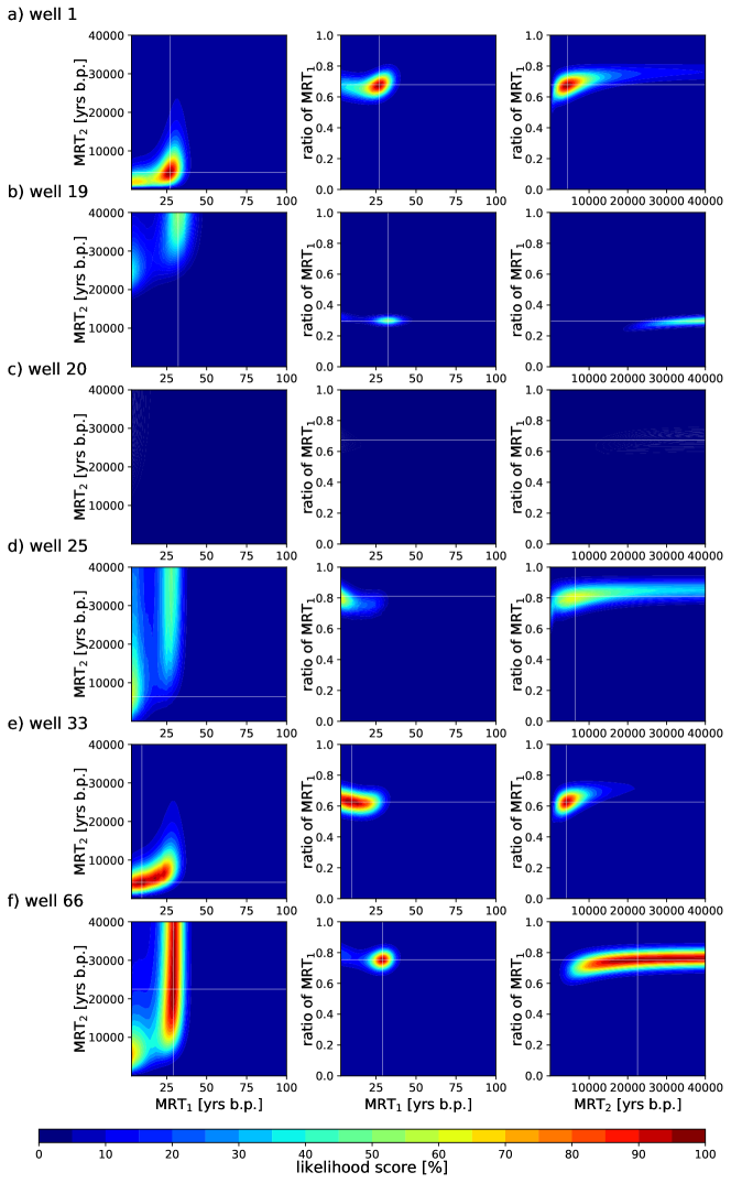
While the MCMC algorithm is designed to find the point of maximum likelihood, a thorough uncertainty analysis is required to understand error margins and codependencies of the parameters. Consequently, the entire distribution along the parameter axes is shown in Figure 5. The values were calculated by screening along parameter surfaces intersecting the point of maximum likelihood, with step sizes y, y and . The points of maximum likelihoods are marked with crosshairs and correspond to the parameter estimates listed in Table 1.
In the left plots where both MRTs are contrasted, two maxima are visible for most wells. Presumably, this stems from the non-monotonic CFC-11 input curve yielding too high concentrations for y y which can be verified in the Dispersion Model trajectories for CFC-11 in Figures 2 and 3. This effect explains the clustering of the estimates for MRT1 mentioned above.
The maxima of the likelihood score in parameter space are well-defined regarding MRT1 and the ratio whereas MRT2 has very large tolerance towards the upper age end (revealing the slow exponential decay of 14C, the only tracer applicable in this regime). This is most evident for well 66 where any value for MRT2 between 10000 and 40000 years yields a high likelihood score. While this appears favorable, the associated error boundaries are respectively large. Worse still for well 25, the blurred likelihood profile results in error margins spanning the entire parameter range of MRT2 (compare Table 1). For well 20, the likelihood score does not reach a high enough level to be resolved in the applied color scale. However, the contour lines and the crosshairs indicate the location of the maximum.
For most wells, only parts of the parameter space exhibit notable likelihoods. However, the \changeconstraintsboundaries were not adjusted individually to allow for comparison between the wells. This impacts the model’s performance which is discussed in the following section.
3.5 Model comparison
The findings of the nonparametric model given the predefined bin boundaries are generally in agreement with the DMmix parameter estimates. In addition to evaluating the tracer data, quantitative measures are required for an adequate model comparison. Therefore, several indicators regarding the models are \change[author]opposedcontrasted in Table 2.
3.5.1 Maximum likelihood score
One measure to evaluate the models’ performance is the maximum likelihood as well as the score, which on average is slightly higher for the nonparametric model than for DMmix. For wells 20, 33 and 66, the results of the applied models are almost identical. While both models reproduce the CFC-11 values of the three remaining wells almost perfectly, their performance diverges in respect to the 14C and 39Ar values. Looking at the 14C to 39Ar relationship, it becomes apparent that the nonparametric model struggles in reproducing a high ratio (well 1) and the DMmix model in reproducing a low ratio (wells 19 and 25). Possible reasons for the different behaviour may be a different weighting of the 14C bomb peak or the discrete steps of the nonparametric model between bins. Another explanation is the ability of the nonparametric model to produce lower 14C concentrations due to the chosen model constraints and with that, a more efficient dilution of the entire sample with 14C-dead water. In addition, wells 19 and 25 are the only two wells for which the choice of Péclet number 10 for the DMmix model may hinder the maximum likelihood (compare Figure S4 \add[author]in the Supporting Information). Nevertheless, for reasons of simplicity and consistency, the same Péclet numbers were chosen for all wells and components.
3.5.2 Bayes Factor
The second quantity to be analyzed is the Bayes factor , a measure for the mean likelihood in parameter space. For all wells, the Bayes factor for DMmix is slightly higher than for the nonparametric model, indicating that DMmix performs better (compare Table 2). For both models and most wells, the average log-likelihood is between 0.5 and 2. Only well 20 yields a considerably lower Bayes Factor, as presumed from Figure 5. A good Bayes Factor is achieved for models with a clever prior selection (or, in this study, an advised choice of the parameter constraints). Hence, the 5-dimensional parameter space of the nonparametric model harbors more sectors of low likelihood than the 3-dimensional parameter space of DMmix. However, under the perspective of equity, it is essential to mention that the parameter constraints of the mean residence times in DMmix were designed based on results of the nonparametric model. In particular, MRT1 with its upper limit of 100 y is able to avoid vast stretches of redundant parameter space, making possible a faster computation in MCMC, a higher precision and, manifestly, a better Bayes Factor. Comparing the different wells, well 19 yields the best results for the DMmix model while for the nonparametric model, it is only ranked fourth after wells 33, 66 and 1. This effect again displays the higher likelihood for lower measurement uncertainties (compare Table DS01) and contrasts the impression from Figure 5 where the likelihood score is illustrated.
3.5.3 Leave-one-out cross validation
The third quantity listed in Table 2 is the expected log likelihood for leave-one-out (LOO) cross validation. With , overfitting is penalized by making predictions on data not used during the training of the model. Analogous to the Bayes Factor, the results of both models are in the same order of magnitude, but with an opposite trend; more precisely, the nonparametric 6-bin model performs better than the DMmix model for all wells. This is surprising as the nonparametric model involves a higher number of free parameters, a key quantity applied to estimate overfitting in other model performance approaches. This reveals that for this study, the number of free parameters is not the pivotal measure to rate the models’ predictive performance. On the contrary, the DMmix model seems to be more capable to tailor a water mixture producing specific tracer concentrations while the nonparametric model is bound to its uniform age contributions within each bin, hindering its flexibility with regard to far-fetched model outcomes. As a result, the likelihood in parameter space produced with and without one of the tracers are more in accordance with each other for the nonparametric model.
Among the wells, the DMmix model ranks well 66 first while for the nonparametric model, well 25 performs best. Besides the exact order of the well-performing wells, a similar trend is visible for both models with the of well 19 being significantly lower and well 20 taking the last place. This result is not unexpected as for both wells, the 14C and 39Ar results are not in accordance. For incompatible tracer measurements, a procedure based on leaving out one tracer at a time and evaluating the result with respect to this tracer will evidently distort the image more drastically and produce poor likelihoods. Additionally, LOO results can also be visualized to see the effect of the individual tracers on the parameter estimates (compare Figure S5 in the Supporting Information).
| Well | max. lik | max. lik score [] | Bayes factor | |||||
|---|---|---|---|---|---|---|---|---|
| DMmix | nonpar | DMmix | nonpar | DMmix | nonpar | DMmix | nonpar | |
| 1 | 536 | 478 | 100.0 | 89.2 | 1.641 | 1.236 | 2.02 | 2.38 |
| 19 | 1885 | 2983 | 52.6 | 83.2 | 2.027 | 0.758 | 0.34 | 0.87 |
| 20 | 0.79 | 0.33 | 0.1 | 0.1 | -6.638 | -8.465 | -15.62 | -12.92 |
| 25 | 295 | 395 | 67.7 | 90.6 | 1.382 | 0.594 | 2.49 | 3.88 |
| 33 | 562 | 561 | 100.0 | 99.8 | 2.001 | 1.999 | 2.88 | 3.57 |
| 66 | 393 | 393 | 100.0 | 100.0 | 1.939 | 1.596 | 3.00 | 3.73 |
4 Discussion
4.1 Intercomparison of the findings
While several tracers measured in the campaign were not applied for Bayesian modelling, their qualitative evidence can be compared with the model outcomes. As all measurements of CFC-113 and several SF6 concentrations indicate contamination in the respective wells, no relevant findings arise from those tracers worth comparing with modelling results. For CFC-12, the parameter estimates attained in the modelling approach could be applied to calculate the CFC-12 concentrations and tracer likelihoods which are displayed in Table S2 (Supporting Information). As expected based on the CFC-12 vs. CFC-11 plot in Figure 2, for most wells CFC-12 results generally convey a similar picture with slightly different likelihoods. Wells 19 and 25 form an exception as they yield poor CFC-12 likelihoods due to the large difference between CFC-11 and CFC-12 concentrations.
From 4Herad results, well 1 would be inferred the oldest well by far (compare Figure 2). Instead, well 1 exhibits the youngest mean residence times (or higher ratios in young age bins for the nonparametric model). The high radiogenic helium at well 1 can possibly be explained by the geology. The coastal plain is strongly characterized by uplift and erosion, visible, for example, on the different layers that wedge out on the surface. In the area of well 1, Cretaceous layers are exposed, while Paleocene layers are pending towards the West [Khalifa (\APACyear1988)]. \change[author]Hence,The low measured 3He/4He ratio of 0.08 Ra in well 1 indicates a purely crustal He origin, which could be due to locally enhanced U and Th concentrations in the rocks or the presence of a fault channeling the crustal He flux at this location. In either case, it is likely a local phenomenon and the enigma of repeated excessive radiogenic helium measurements in the Eastern Salalah Plain cannot be solved in this study. However, the impression that wells 25 and 33 are among the youngest is supported by the modelling results.
4.2 Critical assessment of the applied methods
In the context of the model, up to five parameters estimates are calculated with only a set of three tracers. To assure a sufficiently determined system, it is essential to evaluate results from repeated execution with respect to their reproducibility. While the optimization process with six bins (five free parameters) in the nonparametric model proves to be reliable, increasing the number of bins to seven bins (six free parameters) leads to poor reproducibility of the estimates. Hence, the choice of a six-bin model arises from the highest age resolution under simultaneous consideration of a reliable estimation process. For the DMmix model, however, a possible underdetermination was prevented by reducing the parameters to only MRT1, MRT2 and the ratio by separately evaluating the two Péclet numbers.
To reduce the risk of contamination, predominantly wells located along the front of the Dhofar mountains upstream of agricultural and residential areas were chosen. Only well 19 poses the danger of infiltrated irrigation water as it is situated further downstream amid agricultural area. However, there is no indication of anthropogenic contamination in well 19 and its location further down the flow path is reflected in a higher MRT2 and a lower ratio of the young component, compared to the other wells. For well 20, the very high 39Ar results contradicting the CFC-11 and 14C measurements may have been caused by a contamination of the sample. Subsurface production of 39Ar [Florkowski (\APACyear1992)] can be excluded as the Salalah Plain does not exhibit a high granite content [Khalifa (\APACyear1988)]. Noteworthy, despite incomplete data on well properties, well 20 seems to exhibit an excessively long screen and the pump was placed near the surface. Hence, despite thorough flushing before sampling, the inconsistent tracer data may be ascribed to stagnant water in the samples.
Assessing the credibility of the tracers involved in the Bayesian modelling approach leads to wide differences between 14C, 39Ar and CFC-11. For 14C, the tracer stipulating the old range, all correction methods involving the groundwater chemistry or C failed, leaving only the Vogel model as an empirical estimate. Combined with its high reactivity and subjection to fractionation, this does not inspire a high level of confidence for this tracer which was taken into account by assigning an uncertainty of 5 % to the Vogel correction. \add[author]On top of this uncertainty, it is possible that an appropriate C-based correction would substantially reduce the 14C ages for wells 19 and 20, thereby reducing discrepancies to the other tracers as well as the contributions of the oldest age bins to the TTDs of these wells. 39Ar, on the other hand, is not involved in geochemical processes and no fractionation processes need to be considered, making it the most robust tracer in the study. CFC concentrations may be altered by contamination arising from industrial activities, leaking landfills or sewage lines and effects from irrigation or pesticides [Darling \BOthers. (\APACyear2012), IAEA (\APACyear2006), Oster \BOthers. (\APACyear1996)]. In addition, the sampling tubing was stored in contact with atmospheric air, potentially allowing CFCs to diffuse into the material. These effects affect the individual CFCs differently and with CFC-11, the most trustworthy of the three tracers given the measurement results was chosen.
In contrast to their differing reliability, all three tracers contribute to the total likelihood in equal shares. The individual tracer likelihoods are substantially governed by the measurement errors of the tracers, allowing considerably higher deviance between modelled and measured activity of 39Ar than for the other tracers. This is most evident for well 20 where modelled and measured 14C activities are similar while for 39Ar they differ widely, despite reliability considerations. This can be taken into account by quantifying a level of reliability for the individual tracers resulting in weight factors for the tracer likelihoods. In lack of a quantification of the tracer reliability, this step was renounced in this study.
In addition to the maximum likelihood achievable within a model, the models’ performance can be rated. While the DMmix model yields better results for the Bayes Factor, the nonparametric model proves a better predictive adequacy in leave-one-out cross validation. From a methods perspective, calculation of the Bayes Factor is highly cost intensive in terms of computation time. Worse still is as the integral of the posterior and likelihood is evaluated over the whole parameter space. For application in further studies this method is not recommended by the authors if computational power is a limited resource. Furthermore, a leave-one-out procedure may be more suitable for a system with more than three tracers. Most notably, leaving out 14C leaves a major part of the parameter space unresolved (compare Figure S5 in the Supporting Information), which obviously yields results eminently different to those modelled with all three tracers.
4.3 Hydrological interpretation
Taking the parameter estimates as the ’true’ representation of the hydrological setting, the results of the sampled wells can be employed to assess the groundwater system in the Salalah Plain. From preliminary studies, groundwater ages in the range of decades up to centuries were expected [I. Clark \BOthers. (\APACyear1987)], with slightly lower ages in the central plain due to a higher flow rate [GRC (\APACyear2004)]. In this study, however, all wells (excluding well 20 due to poor goodness of fit) yield a conclusive picture of the composition with regard to two distinct water masses of very young ( y) and very old origin ( y). The ratio and the exact ages, however, differ widely among the wells, potentially due to the difference of the locations in East-West direction and along flow lines (compare Figure 1). The high ratio of young water could be an indication of a short distance between the infiltration site and the well or fast flow paths, both in combination with only shallow infiltration. During the monsoon and especially during extreme events with large-scale flooding, rain or water that has accumulated in ponds and depressions may infiltrate in the immediate vicinity of the well. Before 2018, Cyclone Keila (2011) was the last storm bringing large amounts of rain to the Arabian South coast and flooding large parts of the plain for several days [Strauch \BOthers. (\APACyear2014)]. Besides seasonal or extreme events, there is a continuous inflow from the mountains into the coastal aquifer driven by more than 500 m difference in groundwater head. In this baseflow, mixing of water with short and long flow paths takes place, especially at the outlet - the transition from mountain aquifer to coastal aquifer where the thickness of the water bearing horizon decreases.
5 Conclusion
In this study the groundwater system of the Salalah Plain in Southern Oman was investigated by modelling transit time distributions based on a Bayesian multi-tracer approach. The results show that it is possible to model the measured concentrations of 14C, 39Ar and CFC-11 with TTDs of different shape using Bayesian statistics. The applied models, a two-component Dispersion Model (DMmix) and a shape-free nonparametric model with six bins, were compared with respect to their maximum likelihood, the Bayes Factor and the leave-one-out expected log likelihood. On average, the nonparametric model performed slightly better in terms of maximum likelihood and leave-one-out cross validation while the Bayes Factor was minimally lower than in the DMmix model. All wells exhibited age distributions of two clusters with a large gap in between, indicating water below 30 y and beyond 1000 y. While the occurrence of two peaks in the age distribution of groundwater has been found in other studies as well [Broers \BOthers. (\APACyear2021), McCallum \BOthers. (\APACyear2017)], the extreme age difference observed here seems unusual and may be related to the rather special hydrogeological and climatic conditions of the Salalah Plain.
Those findings play a crucial role in the estimation of the renewal rate of the groundwater in the Salalah Plain which is currently abstracted in high amounts and constitutes an indispensable resource for agricultural production. To close the gaps of this study, more sampling campaigns in the study area including soil characteristics for a more evidence-based 14C correction as well as a deeper understanding of the well structure related to the aquifer are required. In addition, the MCMC methods may be replaced by a faster strategy like evolutionary algorithms [Holland (\APACyear1992), Turing (\APACyear1950)] to allow for a wider applicability of the Bayesian modelling software in other environmental studies.
Acknowledgements.
This work was supported by the Deutsche Forschungsgemeinschaft in the joint projects AE 93/14-1 and OB 164/11-1, as well as the project ’Submarine Groundwater Discharge: Adaption of an Autonomous Aquatic Vehicle for Robotic Measurements, Sampling and Monitoring’, funded by The Research Council of Oman (TRC Research Contract No. TRC/RCP/15/001). We kindly acknowledge steady support by the Ministry of Agriculture, Fisheries and Water Resources of the Sultanate of Oman. We thank Fynn Bachmann, Dominik Lorenz and Michael Aichmüller for useful discussions.References
- Ahmed \BBA Choudri (\APACyear2012) \APACinsertmetastarAhmed2012{APACrefauthors}Ahmed, M.\BCBT \BBA Choudri, B\BPBIS. \APACrefYearMonthDay2012nov. \BBOQ\APACrefatitleClimate change in Oman: Current knowledge and way forward Climate change in Oman: Current knowledge and way forward.\BBCQ \APACjournalVolNumPagesEducation, Business and Society: Contemporary Middle Eastern Issues54228–236. {APACrefDOI} 10.1108/17537981211284416 \PrintBackRefs\CurrentBib
- Akaike (\APACyear1973) \APACinsertmetastarAkaike1973{APACrefauthors}Akaike, H. \APACrefYearMonthDay1973. \BBOQ\APACrefatitleInformation theory and an extension of the maximum likelihood principle Information theory and an extension of the maximum likelihood principle.\BBCQ \BIn B\BPBIN. Petrov \BBA B\BPBIF. Csaki (\BEDS), \APACrefbtitleSecond International Symposium on Information Theory Second international symposium on information theory (\BPGS 267–281). \APACaddressPublisherBudapestAcademiai Kiado. \PrintBackRefs\CurrentBib
- Al-Ajmi (\APACyear2018) \APACinsertmetastarAl-Ajmi2018{APACrefauthors}Al-Ajmi, D\BPBIN. \APACrefYearMonthDay2018oct. \BBOQ\APACrefatitleClimate Aridity: The Sultanate of Oman as a Case Study Climate Aridity: The Sultanate of Oman as a Case Study.\BBCQ \APACjournalVolNumPagesInternational Journal of Earth Science and Geology111–3. {APACrefDOI} 10.18689/ijeg-1000101 \PrintBackRefs\CurrentBib
- Al-Ajmi \BOthers. (\APACyear2013) \APACinsertmetastarAl-Ajmi2013{APACrefauthors}Al-Ajmi, D\BPBIN., Idrees, A\BPBIM.\BCBL \BBA Al-Hatrushi, S. \APACrefYearMonthDay2013. \BBOQ\APACrefatitleSpatial and Temporal Analysis of Recurrence Time of Rainfall in the Sultanate of Oman Spatial and Temporal Analysis of Recurrence Time of Rainfall in the Sultanate of Oman.\BBCQ \APACjournalVolNumPagesBritish Journal of Arts and Social Sciences121. \PrintBackRefs\CurrentBib
- Al-Habsi \BOthers. (\APACyear2014) \APACinsertmetastarAl-Habsi2014{APACrefauthors}Al-Habsi, M., Gunawardhana, L.\BCBL \BBA Al-Rawas, G. \APACrefYearMonthDay2014. \BBOQ\APACrefatitleTrend Analysis of Climate Variability in Salalah, Oman Trend Analysis of Climate Variability in Salalah, Oman.\BBCQ \APACjournalVolNumPagesInternational Journal of Students’ Research in Technology and Management205168–171. \PrintBackRefs\CurrentBib
- Al-Mashaikhi (\APACyear2011) \APACinsertmetastarAl-Mashaikhi2011{APACrefauthors}Al-Mashaikhi, K\BPBIS\BPBIA. \APACrefYear2011. \APACrefbtitleEvaluation of groundwater recharge in Najd aquifers using hydraulics, hydrochemical and isotope evidences (PhD Thesis) Evaluation of groundwater recharge in Najd aquifers using hydraulics, hydrochemical and isotope evidences (PhD Thesis). \APACaddressPublisherJena. \PrintBackRefs\CurrentBib
- Al-Sarmi \BOthers. (\APACyear2017) \APACinsertmetastarAl-Sarmi2017{APACrefauthors}Al-Sarmi, S., Al-Yahyai, S., Al-Maskari, J., Charabi, Y.\BCBL \BBA Choudri, B\BPBIS. \APACrefYearMonthDay2017. \BBOQ\APACrefatitleRecent Observed Climate Change Over Oman Recent Observed Climate Change Over Oman.\BBCQ \BIn \APACrefbtitleWater resources in arid areas: The way forward Water resources in arid areas: The way forward (\BPGS 89–100). \APACaddressPublisherSpringer International Publishing. {APACrefDOI} 10.1007/978-3-319-51856-5_6 \PrintBackRefs\CurrentBib
- Askri \BOthers. (\APACyear2016) \APACinsertmetastarAskri2016a{APACrefauthors}Askri, B., Ahmed, A\BPBIT., Al-Shanfari, R\BPBIA., Bouhlila, R.\BCBL \BBA Al-Farisi, K\BPBIB\BPBIK. \APACrefYearMonthDay2016jun. \BBOQ\APACrefatitleIsotopic and geochemical identifications of groundwater salinisation processes in Salalah coastal plain, Sultanate of Oman Isotopic and geochemical identifications of groundwater salinisation processes in Salalah coastal plain, Sultanate of Oman.\BBCQ \APACjournalVolNumPagesChemie der Erde762243–255. {APACrefDOI} 10.1016/J.CHEMER.2015.12.002 \PrintBackRefs\CurrentBib
- Bates \BBA Campbell (\APACyear2001) \APACinsertmetastarBates2001{APACrefauthors}Bates, B\BPBIC.\BCBT \BBA Campbell, E\BPBIP. \APACrefYearMonthDay2001apr. \BBOQ\APACrefatitleA Markov chain Monte Carlo scheme for parameter estimation and inference in conceptual rainfall-runoff modeling A Markov chain Monte Carlo scheme for parameter estimation and inference in conceptual rainfall-runoff modeling.\BBCQ \APACjournalVolNumPagesWater Resources Research374937–947. {APACrefDOI} 10.1029/2000WR900363 \PrintBackRefs\CurrentBib
- Bawain (\APACyear2012) \APACinsertmetastarBawain2012{APACrefauthors}Bawain, A\BPBIM\BPBIA. \APACrefYear2012. \APACrefbtitleInfluence of Vegetation on Water Fluxes at the Ground Level in a Semi-arid Cloud Forest in Oman Influence of Vegetation on Water Fluxes at the Ground Level in a Semi-arid Cloud Forest in Oman \APACtypeAddressSchoolPhD Thesis. \APACaddressSchoolFriedrich-Schiller Universität Jena. \PrintBackRefs\CurrentBib
- Bear \BBA Cheng (\APACyear1999) \APACinsertmetastarBear1999a{APACrefauthors}Bear, J.\BCBT \BBA Cheng, A\BPBIH\BHBID. \APACrefYearMonthDay1999. \BBOQ\APACrefatitleSeawater Intrusion in Coastal Aquifers: Concepts, Methods and Practices Seawater Intrusion in Coastal Aquifers: Concepts, Methods and Practices.\BBCQ \BIn (\BPGS 1–8). {APACrefDOI} 10.1007/978-94-017-2969-7_1 \PrintBackRefs\CurrentBib
- Beyersdorfer (\APACyear2016) \APACinsertmetastarBeyersdorfer2016{APACrefauthors}Beyersdorfer, S. \APACrefYear2016. \APACrefbtitleArgon extraction from glacier ice and ocean water for dating with 39Ar-ATTA (Master Thesis) Argon extraction from glacier ice and ocean water for dating with 39Ar-ATTA (Master Thesis). \APACaddressPublisherHeidelberg. \PrintBackRefs\CurrentBib
- Broers \BOthers. (\APACyear2021) \APACinsertmetastarBroers2021{APACrefauthors}Broers, H\BPBIP., Sültenfuß, J., Aeschbach, W., Kersting, A., Menkovich, A., de Weert, J.\BCBL \BBA Castelijns, J. \APACrefYearMonthDay2021jul. \BBOQ\APACrefatitlePaleoclimate Signals and Groundwater Age Distributions From 39 Public Water Works in the Netherlands; Insights From Noble Gases and Carbon, Hydrogen and Oxygen Isotope Tracers Paleoclimate Signals and Groundwater Age Distributions From 39 Public Water Works in the Netherlands; Insights From Noble Gases and Carbon, Hydrogen and Oxygen Isotope Tracers.\BBCQ \APACjournalVolNumPagesWater Resources Research577. {APACrefDOI} 10.1029/2020WR029058 \PrintBackRefs\CurrentBib
- Busenberg \BBA Plummer (\APACyear2000) \APACinsertmetastarBusenberg2000{APACrefauthors}Busenberg, E.\BCBT \BBA Plummer, L\BPBIN. \APACrefYearMonthDay2000oct. \BBOQ\APACrefatitleDating young groundwater with sulfur hexafluoride: Natural and anthropogenic sources of sulfur hexafluoride Dating young groundwater with sulfur hexafluoride: Natural and anthropogenic sources of sulfur hexafluoride.\BBCQ \APACjournalVolNumPagesWater Resources Research36103011–3030. {APACrefDOI} 10.1029/2000WR900151 \PrintBackRefs\CurrentBib
- Cappé \BOthers. (\APACyear2002) \APACinsertmetastarCappe2002{APACrefauthors}Cappé, O., Douc, R., Moulines, E.\BCBL \BBA Robert, C. \APACrefYearMonthDay2002. \BBOQ\APACrefatitleOn the Convergence of the Monte Carlo Maximum Likelihood Method for Latent Variable Models on JSTOR On the Convergence of the Monte Carlo Maximum Likelihood Method for Latent Variable Models on JSTOR.\BBCQ \APACjournalVolNumPagesScandinavian Journal of Statistics294615–635. \PrintBackRefs\CurrentBib
- Chen \BOthers. (\APACyear1999) \APACinsertmetastarChen1999{APACrefauthors}Chen, C\BPBIY., Li, Y\BPBIM., Bailey, K., O’Connor, T\BPBIP., Young, L.\BCBL \BBA Lu, Z\BHBIT. \APACrefYearMonthDay1999nov. \BBOQ\APACrefatitleUltrasensitive Isotope Trace Analyses with a Magneto-Optical Trap Ultrasensitive Isotope Trace Analyses with a Magneto-Optical Trap.\BBCQ \APACjournalVolNumPagesScience28654421139–1141. {APACrefDOI} 10.1126/SCIENCE.286.5442.1139 \PrintBackRefs\CurrentBib
- Cirpka \BOthers. (\APACyear2007) \APACinsertmetastarCirpka2007{APACrefauthors}Cirpka, O\BPBIA., Fienen, M\BPBIN., Hofer, M., Hoehn, E., Tessarini, A., Kipfer, R.\BCBL \BBA Kitanidis, P\BPBIK. \APACrefYearMonthDay2007may. \BBOQ\APACrefatitleAnalyzing Bank Filtration by Deconvoluting Time Series of Electric Conductivity Analyzing Bank Filtration by Deconvoluting Time Series of Electric Conductivity.\BBCQ \APACjournalVolNumPagesGround Water453318–328. {APACrefDOI} 10.1111/j.1745-6584.2006.00293.x \PrintBackRefs\CurrentBib
- I. Clark \BOthers. (\APACyear1987) \APACinsertmetastarClark_1987{APACrefauthors}Clark, I., Fritz, P., Quinn, O., Rippon, P., Nash, H.\BCBL \BBA Al Said, S. \APACrefYearMonthDay1987. \BBOQ\APACrefatitleModern and fossil groundwater in an arid environment: a look at the hydrogeology of Southern Oman Modern and fossil groundwater in an arid environment: a look at the hydrogeology of Southern Oman.\BBCQ \APACjournalVolNumPagesIsotope techniques in water resources development167–187. \PrintBackRefs\CurrentBib
- I\BPBID. Clark \BBA Fritz (\APACyear1997\APACexlab\BCnt1) \APACinsertmetastarClark1997_Trit{APACrefauthors}Clark, I\BPBID.\BCBT \BBA Fritz, P. \APACrefYearMonthDay1997\BCnt1. \BBOQ\APACrefatitleIdentifying and Dating Modern Groundwater Identifying and Dating Modern Groundwater.\BBCQ \BIn \APACrefbtitleEnvironmental isotopes in hydrology Environmental isotopes in hydrology (\BCHAP 7). \PrintBackRefs\CurrentBib
- I\BPBID. Clark \BBA Fritz (\APACyear1997\APACexlab\BCnt2) \APACinsertmetastarClark_1997{APACrefauthors}Clark, I\BPBID.\BCBT \BBA Fritz, P. \APACrefYearMonthDay1997\BCnt2. \BBOQ\APACrefatitleTracing the carbon cycle Tracing the carbon cycle.\BBCQ \BIn \APACrefbtitleEnvironmental isotopes in hydrology Environmental isotopes in hydrology (\BCHAP 5). \PrintBackRefs\CurrentBib
- J\BPBIS. Clark (\APACyear2005) \APACinsertmetastarClark2005{APACrefauthors}Clark, J\BPBIS. \APACrefYearMonthDay2005jan. \APACrefbtitleWhy environmental scientists are becoming Bayesians Why environmental scientists are becoming Bayesians (\BVOL 8) (\BNUM 1). \APACaddressPublisherJohn Wiley and Sons, Ltd. {APACrefDOI} 10.1111/j.1461-0248.2004.00702.x \PrintBackRefs\CurrentBib
- Dames and Moore International (\APACyear1992) \APACinsertmetastarDandMI1992{APACrefauthors}Dames and Moore International. \APACrefYearMonthDay1992. \APACrefbtitleWater and wastewater masterplan for Salalah. Water and wastewater masterplan for Salalah. \APACaddressPublisherOffice of the Minister of State and Governor of Dhofar, Sultanate of Oman. \PrintBackRefs\CurrentBib
- Darling \BOthers. (\APACyear2012) \APACinsertmetastarDarling2012{APACrefauthors}Darling, W\BPBIG., Gooddy, D\BPBIC., MacDonald, A\BPBIM.\BCBL \BBA Morris, B\BPBIL. \APACrefYearMonthDay2012. \BBOQ\APACrefatitleThe practicalities of using CFCs and SF6 for groundwater dating and tracing The practicalities of using CFCs and SF6 for groundwater dating and tracing.\BBCQ \APACjournalVolNumPagesApplied Geochemistry279. {APACrefDOI} 10.1016/j.apgeochem.2012.02.005 \PrintBackRefs\CurrentBib
- Draper (\APACyear1995) \APACinsertmetastarDraper1995{APACrefauthors}Draper, D. \APACrefYearMonthDay1995jan. \BBOQ\APACrefatitleAssessment and Propagation of Model Uncertainty Assessment and Propagation of Model Uncertainty.\BBCQ \APACjournalVolNumPagesJournal of the Royal Statistical Society: Series B (Methodological)57145–70. {APACrefDOI} 10.1111/j.2517-6161.1995.tb02015.x \PrintBackRefs\CurrentBib
- Ebser (\APACyear2018) \APACinsertmetastarEbser2018{APACrefauthors}Ebser, S. \APACrefYear2018. \APACrefbtitleDating of ice and ocean samples with Atom Trap Trace Analysis of 39Ar Dating of ice and ocean samples with Atom Trap Trace Analysis of 39Ar \APACtypeAddressSchoolPhD Thesis. \APACaddressSchoolHeidelberg University. \PrintBackRefs\CurrentBib
- Ebser \BOthers. (\APACyear2018) \APACinsertmetastarEbserPaper{APACrefauthors}Ebser, S., Kersting, A., Stöven, T., Feng, Z., Ringena, L., Schmidt, M.\BDBLOberthaler, M\BPBIK. \APACrefYearMonthDay2018. \BBOQ\APACrefatitleAr dating with small samples provides new key constraints on ocean ventilation Ar dating with small samples provides new key constraints on ocean ventilation.\BBCQ \APACjournalVolNumPagesNature Communications9. {APACrefDOI} 10.1038/s41467-018-07465-7 \PrintBackRefs\CurrentBib
- Engeland \BOthers. (\APACyear2002) \APACinsertmetastarEngeland2002{APACrefauthors}Engeland, K., Gottschalk, L., Engeland, K.\BCBL \BBA Gottschalk, L. \APACrefYearMonthDay2002. \BBOQ\APACrefatitleBayesian estimation of parameters in a regional hydrological model Bayesian estimation of parameters in a regional hydrological model.\BBCQ \APACjournalVolNumPagesEuropean Geosciences Union65883–898. \PrintBackRefs\CurrentBib
- Feng \BOthers. (\APACyear2019) \APACinsertmetastarFeng2019{APACrefauthors}Feng, Z., Bohleber, P., Ebser, S., Ringena, L., Schmidt, M., Kersting, A.\BDBLOberthaler, M\BPBIK. \APACrefYearMonthDay2019nov. \BBOQ\APACrefatitleDating glacier ice of the last millennium by quantum technology Dating glacier ice of the last millennium by quantum technology.\BBCQ \APACjournalVolNumPagesProceedings of the National Academy of Sciences of the United States of America116188781–8786. \PrintBackRefs\CurrentBib
- Flint \BBA Rippon (\APACyear1986) \APACinsertmetastarFlint1986{APACrefauthors}Flint, R.\BCBT \BBA Rippon, P. \APACrefYearMonthDay1986. \BBOQ\APACrefatitleGeological Reassessment of the Salalah plain aquifer Geological Reassessment of the Salalah plain aquifer.\BBCQ \APACjournalVolNumPagesCouncil for conservation of environment and water resources. \PrintBackRefs\CurrentBib
- Florkowski (\APACyear1992) \APACinsertmetastarFlorkowski1992{APACrefauthors}Florkowski, T. \APACrefYearMonthDay1992. \BBOQ\APACrefatitleNatural production of radioactive noble gases in the geosphere Natural production of radioactive noble gases in the geosphere.\BBCQ \APACjournalVolNumPagesIsotopes of noble gases as tracers in environmental studies. \PrintBackRefs\CurrentBib
- Friesen \BOthers. (\APACyear2018) \APACinsertmetastarFriesen2018{APACrefauthors}Friesen, J., Zink, M., Bawain, A.\BCBL \BBA Müller, T. \APACrefYearMonthDay2018. \BBOQ\APACrefatitleHydrometeorology of the Dhofar cloud forest and its implications for groundwater recharge Hydrometeorology of the Dhofar cloud forest and its implications for groundwater recharge.\BBCQ \APACjournalVolNumPagesJournal of Hydrology: Regional Studies1654–66. {APACrefDOI} 10.1016/j.ejrh.2018.03.002 \PrintBackRefs\CurrentBib
- Gamerman \BBA Lopes (\APACyear2006) \APACinsertmetastarGamerman2006{APACrefauthors}Gamerman, D.\BCBT \BBA Lopes, H\BPBIF. \APACrefYear2006. \APACrefbtitleMarkov Chain Monte Carlo: Stochastic Simulation for Bayesian Inference Markov Chain Monte Carlo: Stochastic Simulation for Bayesian Inference (\PrintOrdinal2 \BEd). \APACaddressPublisherCRC Press. \PrintBackRefs\CurrentBib
- Gelhar \BOthers. (\APACyear1992) \APACinsertmetastarGelhar1992{APACrefauthors}Gelhar, L\BPBIW., Welty, C.\BCBL \BBA Rehfeldt, K\BPBIR. \APACrefYearMonthDay1992jul. \BBOQ\APACrefatitleA critical review of data on field-scale dispersion in aquifers A critical review of data on field-scale dispersion in aquifers.\BBCQ \APACjournalVolNumPagesWater Resources Research2871955–1974. {APACrefDOI} 10.1029/92WR00607 \PrintBackRefs\CurrentBib
- Gelman \BOthers. (\APACyear2013) \APACinsertmetastarGelman2013{APACrefauthors}Gelman, A., Carlin, J\BPBIB., Stern, H\BPBIS., Dunson, D\BPBIB., Vehtari, A.\BCBL \BBA Rubin, D\BPBIB. \APACrefYear2013. \APACrefbtitleBayesian data analysis Bayesian data analysis. \PrintBackRefs\CurrentBib
- Gelman \BOthers. (\APACyear2014) \APACinsertmetastarGelman2014{APACrefauthors}Gelman, A., Hwang, J.\BCBL \BBA Vehtari, A. \APACrefYearMonthDay2014nov. \BBOQ\APACrefatitleUnderstanding predictive information criteria for Bayesian models Understanding predictive information criteria for Bayesian models.\BBCQ \APACjournalVolNumPagesStatistics and Computing246997–1016. {APACrefDOI} 10.1007/s11222-013-9416-2 \PrintBackRefs\CurrentBib
- Geyer \BBA Thompson (\APACyear1992) \APACinsertmetastarGeyer1992{APACrefauthors}Geyer, C\BPBIJ.\BCBT \BBA Thompson, E\BPBIA. \APACrefYearMonthDay1992. \BBOQ\APACrefatitleConstrained Monte Carlo Maximum Likelihood for Dependent Data Constrained Monte Carlo Maximum Likelihood for Dependent Data.\BBCQ \APACjournalVolNumPagesArticle in Journal of the Royal Statistical Society. Series B: Methodological543657–699. {APACrefDOI} 10.2307/2345852 \PrintBackRefs\CurrentBib
- GRC (\APACyear2004) \APACinsertmetastarGeoResourcesConsultancy2004{APACrefauthors}GRC. \APACrefYearMonthDay2004. \APACrefbtitleDetailed water resources management and planning study for the Salalah region Part A, Final report Detailed water resources management and planning study for the Salalah region Part A, Final report \APACbVolEdTR\BTR. \APACaddressInstitutionMuscat, Sultanate of OmanGeo Resources Consultancy, GRC. \PrintBackRefs\CurrentBib
- Gronau \BBA Wagenmakers (\APACyear2019) \APACinsertmetastarGronau2019{APACrefauthors}Gronau, Q\BPBIF.\BCBT \BBA Wagenmakers, E\BHBIJ. \APACrefYearMonthDay2019. \BBOQ\APACrefatitleLimitations of Bayesian Leave-One-Out Cross-Validation for Model Selection Limitations of Bayesian Leave-One-Out Cross-Validation for Model Selection.\BBCQ \APACjournalVolNumPagesComputational Brain and Behavior21–11. {APACrefDOI} 10.1007/s42113-018-0011-7 \PrintBackRefs\CurrentBib
- Gunawardhana \BBA Al-Rawas (\APACyear2016) \APACinsertmetastarGunawardhana2016{APACrefauthors}Gunawardhana, L\BPBIN.\BCBT \BBA Al-Rawas, G\BPBIA. \APACrefYearMonthDay2016dec. \BBOQ\APACrefatitleA comparison of trends in extreme rainfall using 20-year data in three major cities in Oman A comparison of trends in extreme rainfall using 20-year data in three major cities in Oman.\BBCQ \APACjournalVolNumPagesJournal of Engineering Research132137–148. {APACrefDOI} 10.24200/tjer.vol13iss2pp137-148 \PrintBackRefs\CurrentBib
- Hall \BBA Plumb (\APACyear1994) \APACinsertmetastarHall1994{APACrefauthors}Hall, T\BPBIM.\BCBT \BBA Plumb, R\BPBIA. \APACrefYearMonthDay1994. \BBOQ\APACrefatitleAge as a diagnostic of stratospheric transport Age as a diagnostic of stratospheric transport.\BBCQ \APACjournalVolNumPagesJournal of Geophysical Research99D11059. {APACrefDOI} 10.1029/93JD03192 \PrintBackRefs\CurrentBib
- Han \BBA Plummer (\APACyear2016) \APACinsertmetastarHan2016{APACrefauthors}Han, L\BPBIF.\BCBT \BBA Plummer, L\BPBIN. \APACrefYearMonthDay2016jan. \BBOQ\APACrefatitleA review of single-sample-based models and other approaches for radiocarbon dating of dissolved inorganic carbon in groundwater A review of single-sample-based models and other approaches for radiocarbon dating of dissolved inorganic carbon in groundwater.\BBCQ \APACjournalVolNumPagesEarth-Science Reviews152119–142. {APACrefDOI} 10.1016/J.EARSCIREV.2015.11.004 \PrintBackRefs\CurrentBib
- Holland (\APACyear1992) \APACinsertmetastarHolland1992{APACrefauthors}Holland, J. \APACrefYear1992. \APACrefbtitleAdaptation in natural and artificial systems: an introductory analysis with applications to biology, control, and artificial intelligence Adaptation in natural and artificial systems: an introductory analysis with applications to biology, control, and artificial intelligence. \APACaddressPublisherMIT press. \PrintBackRefs\CurrentBib
- IAEA (\APACyear2006) \APACinsertmetastarIAEA_CFCs{APACrefauthors}IAEA. \APACrefYear2006. \APACrefbtitleUse of Chlorofluorocarbons in Hydrology: a Guidebook Use of Chlorofluorocarbons in Hydrology: a Guidebook. \APACaddressPublisherViennaInternational Atomic Energy Agency. \PrintBackRefs\CurrentBib
- IAEA/WMO (\APACyear2021) \APACinsertmetastarIAEA/WMO2021{APACrefauthors}IAEA/WMO. \APACrefYearMonthDay2021. \APACrefbtitleGlobal Network of Isotopes in Precipitation. The GNIP Database. Global Network of Isotopes in Precipitation. The GNIP Database. \PrintBackRefs\CurrentBib
- ICBA (\APACyear2012) \APACinsertmetastarICBA{APACrefauthors}ICBA. \APACrefYearMonthDay2012. \APACrefbtitleOman Salinity Strategy. Oman Salinity Strategy. \APACaddressPublisherMinistry of Agriculture and Fisheries (MAF) Dubai and International Center for Biosaline Agriculture (ICBA), Sultanate of Oman. \PrintBackRefs\CurrentBib
- IPCC (\APACyear2019) \APACinsertmetastarIPCC2019{APACrefauthors}IPCC. \APACrefYearMonthDay2019. \APACrefbtitleSpecial Report on Climate Change and Land: an IPCC special report on climate change, desertification, land degradation, sustainable land management, food security, and greenhouse gas fluxes in terrestrial ecosystems Special Report on Climate Change and Land: an IPCC special report on climate change, desertification, land degradation, sustainable land management, food security, and greenhouse gas fluxes in terrestrial ecosystems \APACbVolEdTR\BTR. \PrintBackRefs\CurrentBib
- Jeffrey (\APACyear1961) \APACinsertmetastarJeffrey1961{APACrefauthors}Jeffrey, H. \APACrefYear1961. \APACrefbtitleThe theory of probability The theory of probability (\PrintOrdinal3 \BEd). \APACaddressPublisherOxford, UKOxford University Press. \PrintBackRefs\CurrentBib
- Ju \BOthers. (\APACyear2020) \APACinsertmetastarJu2020{APACrefauthors}Ju, Y\BPBIJ., Massoudieh, A., Kaown, D., Yoon, Y\BPBIY.\BCBL \BBA Lee, K\BPBIK. \APACrefYearMonthDay2020jul. \BBOQ\APACrefatitleCharacterization of flow dynamics around highly-utilized agricultural wells in a fractured-rock aquifer: Assessment of uncertainties lying on groundwater age-dating Characterization of flow dynamics around highly-utilized agricultural wells in a fractured-rock aquifer: Assessment of uncertainties lying on groundwater age-dating.\BBCQ \APACjournalVolNumPagesJournal of Hydrology586124885. {APACrefDOI} 10.1016/j.jhydrol.2020.124885 \PrintBackRefs\CurrentBib
- Jung \BBA Aeschbach (\APACyear2018) \APACinsertmetastarJung2018{APACrefauthors}Jung, M.\BCBT \BBA Aeschbach, W. \APACrefYearMonthDay2018may. \BBOQ\APACrefatitleA new software tool for the analysis of noble gas data sets from (ground)water A new software tool for the analysis of noble gas data sets from (ground)water.\BBCQ \APACjournalVolNumPagesEnvironmental Modelling and Software103120–130. {APACrefDOI} 10.1016/j.envsoft.2018.02.004 \PrintBackRefs\CurrentBib
- Jurgens \BOthers. (\APACyear2012) \APACinsertmetastarJurgens2012{APACrefauthors}Jurgens, B\BPBIC., Böhlke, J\BPBIK.\BCBL \BBA Eberts, S\BPBIM. \APACrefYearMonthDay2012. \APACrefbtitleTracerLPM (Version 1): An Excel ® Workbook for Interpreting Groundwater Age Distributions from Environmental Tracer Data Techniques and Methods 4-F3 TracerLPM (Version 1): An Excel ® Workbook for Interpreting Groundwater Age Distributions from Environmental Tracer Data Techniques and Methods 4-F3 \APACbVolEdTR\BTR. {APACrefDOI} 10.3133/TM4F3 \PrintBackRefs\CurrentBib
- Kass \BBA Raftery (\APACyear1995) \APACinsertmetastarKass1995{APACrefauthors}Kass, R\BPBIE.\BCBT \BBA Raftery, A\BPBIE. \APACrefYearMonthDay1995. \BBOQ\APACrefatitleBayes factors Bayes factors.\BBCQ \APACjournalVolNumPagesJournal of the American Statistical Association90430773–795. {APACrefDOI} 10.1080/01621459.1995.10476572 \PrintBackRefs\CurrentBib
- Khalifa (\APACyear1988) \APACinsertmetastarKhalifa1988{APACrefauthors}Khalifa, M\BPBII. \APACrefYearMonthDay1988. \APACrefbtitleGeological map of Oman, 1:100,000 Sheet NE-40-9D Salalah. Geological map of Oman, 1:100,000 Sheet NE-40-9D Salalah. \APACaddressPublisherMuscat, Sultanate of OmanMinistry of Petroleum and Minerals - Directorate General of Minerals. \PrintBackRefs\CurrentBib
- Khalil \BBA Rasmussen (\APACyear1989) \APACinsertmetastarKhalil1989{APACrefauthors}Khalil, M\BPBIA.\BCBT \BBA Rasmussen, R\BPBIA. \APACrefYearMonthDay1989. \BBOQ\APACrefatitleThe potential of soils as a sink of chlorofluorocarbons and other man‐made chlorocarbons The potential of soils as a sink of chlorofluorocarbons and other man‐made chlorocarbons.\BBCQ \APACjournalVolNumPagesGeophysical Research Letters167. {APACrefDOI} 10.1029/GL016i007p00679 \PrintBackRefs\CurrentBib
- Kirchner \BOthers. (\APACyear2001) \APACinsertmetastarKirchner2001{APACrefauthors}Kirchner, J\BPBIW., Feng, X.\BCBL \BBA Neal, C. \APACrefYearMonthDay2001dec. \BBOQ\APACrefatitleCatchment-scale advection and dispersion as a mechanism for fractal scaling in stream tracer concentrations Catchment-scale advection and dispersion as a mechanism for fractal scaling in stream tracer concentrations.\BBCQ \APACjournalVolNumPagesJournal of Hydrology2541-482–101. {APACrefDOI} 10.1016/S0022-1694(01)00487-5 \PrintBackRefs\CurrentBib
- Kolanoski (\APACyear2002) \APACinsertmetastarKolanoski2002{APACrefauthors}Kolanoski, H. \APACrefYearMonthDay2002. \BBOQ\APACrefatitleDie Maximum-Likelihood-Methode Die Maximum-Likelihood-Methode.\BBCQ \BIn \APACrefbtitleStatistische Methoden der Datenanalyse Statistische methoden der datenanalyse (\BPGS 59–66). \APACaddressPublisherBerlin. \PrintBackRefs\CurrentBib
- Kuczera \BBA Parent (\APACyear1998) \APACinsertmetastarKuczera1998{APACrefauthors}Kuczera, G.\BCBT \BBA Parent, E. \APACrefYearMonthDay1998nov. \BBOQ\APACrefatitleMonte Carlo assessment of parameter uncertainty in conceptual catchment models: The Metropolis algorithm Monte Carlo assessment of parameter uncertainty in conceptual catchment models: The Metropolis algorithm.\BBCQ \APACjournalVolNumPagesJournal of Hydrology2111-469–85. {APACrefDOI} 10.1016/S0022-1694(98)00198-X \PrintBackRefs\CurrentBib
- Laloy \BOthers. (\APACyear2013) \APACinsertmetastarLaloy2013{APACrefauthors}Laloy, E., Rogiers, B., Vrugt, J\BPBIA., Mallants, D.\BCBL \BBA Jacques, D. \APACrefYearMonthDay2013may. \BBOQ\APACrefatitleEfficient posterior exploration of a high-dimensional groundwater model from two-stage Markov chain Monte Carlo simulation and polynomial chaos expansion Efficient posterior exploration of a high-dimensional groundwater model from two-stage Markov chain Monte Carlo simulation and polynomial chaos expansion.\BBCQ \APACjournalVolNumPagesWater Resources Research4952664–2682. {APACrefDOI} 10.1002/wrcr.20226 \PrintBackRefs\CurrentBib
- Liu \BBA Gupta (\APACyear2007) \APACinsertmetastarLiu2007{APACrefauthors}Liu, Y.\BCBT \BBA Gupta, H\BPBIV. \APACrefYearMonthDay2007jul. \APACrefbtitleUncertainty in hydrologic modeling: Toward an integrated data assimilation framework Uncertainty in hydrologic modeling: Toward an integrated data assimilation framework (\BVOL 43) (\BNUM 7). \APACaddressPublisherJohn Wiley and Sons, Ltd. {APACrefDOI} 10.1029/2006WR005756 \PrintBackRefs\CurrentBib
- Loosli (\APACyear1983) \APACinsertmetastarLoosli1983{APACrefauthors}Loosli, H\BPBIH. \APACrefYearMonthDay1983. \BBOQ\APACrefatitleA dating method with 39Ar A dating method with 39Ar.\BBCQ \APACjournalVolNumPagesEarth and Planetary Science Letters63151–62. {APACrefDOI} 10.1016/0012-821X(83)90021-3 \PrintBackRefs\CurrentBib
- Lu \BOthers. (\APACyear2014) \APACinsertmetastarLu2014{APACrefauthors}Lu, Z\BHBIT., Schlosser, P., Smethie, W., Sturchio, N., Fischer, T., Kennedy, B.\BDBLYokochi, R. \APACrefYearMonthDay2014nov. \BBOQ\APACrefatitleTracer applications of noble gas radionuclides in the geosciences Tracer applications of noble gas radionuclides in the geosciences.\BBCQ \APACjournalVolNumPagesEarth-Science Reviews138196–214. {APACrefDOI} 10.1016/j.earscirev.2013.09.002 \PrintBackRefs\CurrentBib
- Macumber \BOthers. (\APACyear1998) \APACinsertmetastarMacumber1998{APACrefauthors}Macumber, P., Abri, R.\BCBL \BBA Akhzami, S. \APACrefYearMonthDay1998aug. \BBOQ\APACrefatitleHydrochemical facies in the groundwater of central and southern Oman Hydrochemical facies in the groundwater of central and southern Oman.\BBCQ \BIn \APACrefbtitleQuaternary Deserts and Climatic Change Quaternary deserts and climatic change (\BPGS 511–520). \APACaddressPublisherCRC Press. {APACrefURL} https://www.taylorfrancis.com/chapters/edit/10.1201/9781003077862-51/hydrochemical-facies-groundwater-central-southern-oman-macumber-abri-akhzami {APACrefDOI} 10.1201/9781003077862-51 \PrintBackRefs\CurrentBib
- Maloszewski (\APACyear1996) \APACinsertmetastarMaloszewski2000{APACrefauthors}Maloszewski, P. \APACrefYearMonthDay1996. \BBOQ\APACrefatitleLumped parameter models for the interpretation of environmental tracer data Lumped parameter models for the interpretation of environmental tracer data.\BBCQ \BIn \APACrefbtitleIAEA. Iaea. \APACaddressPublisherNeuherbergInternational Atomic Energy Agency. \PrintBackRefs\CurrentBib
- Małoszewski \BBA Zuber (\APACyear1982) \APACinsertmetastarMaloszewski1982{APACrefauthors}Małoszewski, P.\BCBT \BBA Zuber, A. \APACrefYearMonthDay1982jun. \BBOQ\APACrefatitleDetermining the turnover time of groundwater systems with the aid of environmental tracers. 1. Models and their applicability Determining the turnover time of groundwater systems with the aid of environmental tracers. 1. Models and their applicability.\BBCQ \APACjournalVolNumPagesJournal of Hydrology573-4207–231. {APACrefDOI} 10.1016/0022-1694(82)90147-0 \PrintBackRefs\CurrentBib
- Marshall \BOthers. (\APACyear2004) \APACinsertmetastarMarshall2004{APACrefauthors}Marshall, L., Nott, D.\BCBL \BBA Sharma, A. \APACrefYearMonthDay2004. \BBOQ\APACrefatitleA comparative study of Markov chain Monte Carlo methods for conceptual rainfall-runoff modeling A comparative study of Markov chain Monte Carlo methods for conceptual rainfall-runoff modeling.\BBCQ \APACjournalVolNumPagesWater Resources Research402. {APACrefDOI} 10.1029/2003WR002378 \PrintBackRefs\CurrentBib
- Massoudieh \BOthers. (\APACyear2012) \APACinsertmetastarMassoudieh2012{APACrefauthors}Massoudieh, A., Sharifi, S.\BCBL \BBA Solomon, D\BPBIK. \APACrefYearMonthDay2012sep. \BBOQ\APACrefatitleBayesian evaluation of groundwater age distribution using radioactive tracers and anthropogenic chemicals Bayesian evaluation of groundwater age distribution using radioactive tracers and anthropogenic chemicals.\BBCQ \APACjournalVolNumPagesWater Resources Research489. {APACrefURL} http://doi.wiley.com/10.1029/2012WR011815 {APACrefDOI} 10.1029/2012WR011815 \PrintBackRefs\CurrentBib
- Massoudieh \BOthers. (\APACyear2014) \APACinsertmetastarMassoudieh2014{APACrefauthors}Massoudieh, A., Visser, A., Sharifi, S.\BCBL \BBA Broers, H\BPBIP. \APACrefYearMonthDay2014. \BBOQ\APACrefatitleA Bayesian modeling approach for estimation of a shape-free groundwater age distribution using multiple tracers A Bayesian modeling approach for estimation of a shape-free groundwater age distribution using multiple tracers.\BBCQ \APACjournalVolNumPagesApplied Geochemistry50. {APACrefDOI} 10.1016/j.apgeochem.2013.10.004 \PrintBackRefs\CurrentBib
- McCallum \BOthers. (\APACyear2017) \APACinsertmetastarMcCallum2017{APACrefauthors}McCallum, J\BPBIL., Cook, P\BPBIG., Dogramaci, S., Purtschert, R., Simmons, C\BPBIT.\BCBL \BBA Burk, L. \APACrefYearMonthDay2017feb. \BBOQ\APACrefatitleIdentifying modern and historic recharge events from tracer-derived groundwater age distributions Identifying modern and historic recharge events from tracer-derived groundwater age distributions.\BBCQ \APACjournalVolNumPagesWater Resources Research5321039–1056. {APACrefDOI} 10.1002/2016WR019839 \PrintBackRefs\CurrentBib
- McCallum \BOthers. (\APACyear2014) \APACinsertmetastarMcCallum2014{APACrefauthors}McCallum, J\BPBIL., Engdahl, N\BPBIB., Ginn, T\BPBIR.\BCBL \BBA Cook, P\BPBIG. \APACrefYearMonthDay2014mar. \BBOQ\APACrefatitleNonparametric estimation of groundwater residence time distributions: What can environmental tracer data tell us about groundwater residence time? Nonparametric estimation of groundwater residence time distributions: What can environmental tracer data tell us about groundwater residence time?\BBCQ \APACjournalVolNumPagesWater Resources Research5032022–2038. {APACrefDOI} 10.1002/2013WR014974 \PrintBackRefs\CurrentBib
- McGuire \BBA McDonnell (\APACyear2006) \APACinsertmetastarMcGuire2006{APACrefauthors}McGuire, K\BPBIJ.\BCBT \BBA McDonnell, J\BPBIJ. \APACrefYearMonthDay2006nov. \BBOQ\APACrefatitleA review and evaluation of catchment transit time modeling A review and evaluation of catchment transit time modeling.\BBCQ \APACjournalVolNumPagesJournal of Hydrology3303-4543–563. {APACrefDOI} 10.1016/j.jhydrol.2006.04.020 \PrintBackRefs\CurrentBib
- Metropolis \BOthers. (\APACyear1953) \APACinsertmetastarMetropolis1953{APACrefauthors}Metropolis, N., Rosenbluth, A\BPBIW., Rosenbluth, M\BPBIN., Teller, A\BPBIH.\BCBL \BBA Teller, E. \APACrefYearMonthDay1953. \BBOQ\APACrefatitleEquation of State Calculations by Fast Computing Machines Equation of State Calculations by Fast Computing Machines.\BBCQ \APACjournalVolNumPagesStudies in Molecular Dynamics. I. General Method The Journal of Chemical Physics2161208. {APACrefDOI} 10.1063/1.1699114 \PrintBackRefs\CurrentBib
- Morris \BOthers. (\APACyear2006) \APACinsertmetastarMorris2006{APACrefauthors}Morris, B\BPBIL., Darling, W\BPBIG., Gooddy, D\BPBIC., Litvak, R\BPBIG., Neumann, I., Nemaltseva, E\BPBIJ.\BCBL \BBA Poddubnaia, I. \APACrefYearMonthDay2006jan. \BBOQ\APACrefatitleAssessing the extent of induced leakage to an urban aquifer using environmental tracers: An example from Bishkek, capital of Kyrgyzstan, Central Asia Assessing the extent of induced leakage to an urban aquifer using environmental tracers: An example from Bishkek, capital of Kyrgyzstan, Central Asia.\BBCQ \APACjournalVolNumPagesHydrogeology Journal141-2225–243. {APACrefDOI} 10.1007/s10040-005-0441-x \PrintBackRefs\CurrentBib
- Müller \BOthers. (\APACyear2020) \APACinsertmetastarMuller2020{APACrefauthors}Müller, T., Friesen, J., Weise, S\BPBIM., Al Abri, O., Bait Said, A\BPBIB\BPBIA.\BCBL \BBA Michelsen, N. \APACrefYearMonthDay2020dec. \BBOQ\APACrefatitleStable Isotope Composition of Cyclone Mekunu Rainfall, Southern Oman Stable Isotope Composition of Cyclone Mekunu Rainfall, Southern Oman.\BBCQ \APACjournalVolNumPagesWater Resources Research5612. {APACrefDOI} 10.1029/2020WR027644 \PrintBackRefs\CurrentBib
- Newman \BOthers. (\APACyear2010) \APACinsertmetastarNewman2010{APACrefauthors}Newman, B\BPBID., Osenbrück, K., Aeschbach-Hertig, W., Solomon, D\BPBIK., Cook, P., Rózánski, K.\BCBL \BBA Kipfer, R. \APACrefYearMonthDay2010. \BBOQ\APACrefatitleDating of ’young’ groundwaters using environmental tracers: Advantages, applications, and research needs Dating of ’young’ groundwaters using environmental tracers: Advantages, applications, and research needs.\BBCQ \APACjournalVolNumPagesIsotopes in Environmental and Health Studies463259–278. {APACrefDOI} 10.1080/10256016.2010.514339 \PrintBackRefs\CurrentBib
- NOAA (\APACyear2018) \APACinsertmetastarNOAA2018{APACrefauthors}NOAA. \APACrefYearMonthDay2018. \APACrefbtitleGlobal Monitoring Laboratory. Chlorofluorocarbon-11 (combined data set). Global Monitoring Laboratory. Chlorofluorocarbon-11 (combined data set). \PrintBackRefs\CurrentBib
- Oster \BOthers. (\APACyear1996) \APACinsertmetastarOster1996{APACrefauthors}Oster, H., Sonntag, C.\BCBL \BBA Münnich, K\BPBIO. \APACrefYearMonthDay1996. \BBOQ\APACrefatitleGroundwater age dating with chlorofluorocarbons Groundwater age dating with chlorofluorocarbons.\BBCQ \APACjournalVolNumPagesWater Resources Research3210. {APACrefDOI} 10.1029/96WR01775 \PrintBackRefs\CurrentBib
- Ouarda \BBA El-Adlouni (\APACyear2011) \APACinsertmetastarOuarda2011{APACrefauthors}Ouarda, T.\BCBT \BBA El-Adlouni, S. \APACrefYearMonthDay2011jun. \BBOQ\APACrefatitleBayesian Nonstationary Frequency Analysis of Hydrological Variables1 Bayesian Nonstationary Frequency Analysis of Hydrological Variables1.\BBCQ \APACjournalVolNumPagesJAWRA Journal of the American Water Resources Association473496–505. {APACrefDOI} 10.1111/j.1752-1688.2011.00544.x \PrintBackRefs\CurrentBib
- Parno \BBA Marzouk (\APACyear2014) \APACinsertmetastarParno2014{APACrefauthors}Parno, M.\BCBT \BBA Marzouk, Y. \APACrefYearMonthDay2014dec. \BBOQ\APACrefatitleTransport map accelerated Markov chain Monte Carlo Transport map accelerated Markov chain Monte Carlo.\BBCQ \APACjournalVolNumPagesSIAM-ASA Journal on Uncertainty Quantification62645–682. {APACrefDOI} 10.1137/17M1134640 \PrintBackRefs\CurrentBib
- Platel \BOthers. (\APACyear1987) \APACinsertmetastarPlatel1987{APACrefauthors}Platel, J\BPBIP., Qidwai, H\BPBIA.\BCBL \BBA Khalifa, M\BPBII. \APACrefYearMonthDay1987. \APACrefbtitleGeological map of Oman, 1:100,000 Sheet NE-40-9E Marbat. Explanatory notes. Geological map of Oman, 1:100,000 Sheet NE-40-9E Marbat. Explanatory notes. \APACaddressPublisherMuscat, Sultanate of OmanMinistry of Petroleum and Minerals – Directorate General of Minerals. \PrintBackRefs\CurrentBib
- Platel \BOthers. (\APACyear1992) \APACinsertmetastarPlatel1992{APACrefauthors}Platel, J\BPBIP., Roger, J., Peters, T., Mercolli, I., Kramers, J\BPBID.\BCBL \BBA Le Métour, J. \APACrefYearMonthDay1992. \APACrefbtitleGeological Map of Salalah, Sheet NE 40-09, 1: 250000, with explanatory notes. Geological Map of Salalah, Sheet NE 40-09, 1: 250000, with explanatory notes. \APACaddressPublisherDirectorate General of Minerals, Oman Ministry of Petroleum and Minerals. \PrintBackRefs\CurrentBib
- Rädle (\APACyear2019) \APACinsertmetastarRadle2019{APACrefauthors}Rädle, V. \APACrefYear2019. \APACrefbtitleMulti-Tracer Study for Groundwater Dating in Southern Oman (Master Thesis) Multi-Tracer Study for Groundwater Dating in Southern Oman (Master Thesis). \APACaddressPublisherHeidelberg. {APACrefDOI} 10.11588/heidok.00030882 \PrintBackRefs\CurrentBib
- Reza Najafi \BBA Moradkhani (\APACyear2013) \APACinsertmetastarRezaNajafi2013{APACrefauthors}Reza Najafi, M.\BCBT \BBA Moradkhani, H. \APACrefYearMonthDay2013oct. \BBOQ\APACrefatitleAnalysis of runoff extremes using spatial hierarchical Bayesian modeling Analysis of runoff extremes using spatial hierarchical Bayesian modeling.\BBCQ \APACjournalVolNumPagesWater Resources Research49106656–6670. {APACrefDOI} 10.1002/wrcr.20381 \PrintBackRefs\CurrentBib
- Ritterbusch \BOthers. (\APACyear2014) \APACinsertmetastarRitterbusch2014{APACrefauthors}Ritterbusch, F., Ebser, S., Welte, J., Reichel, T., Kersting, A., Purtschert, R.\BDBLOberthaler, M\BPBIK. \APACrefYearMonthDay2014. \BBOQ\APACrefatitleGroundwater dating with Atom Trap Trace Analysis of 39Ar Groundwater dating with Atom Trap Trace Analysis of 39Ar.\BBCQ \APACjournalVolNumPagesGeophysical Research Letters. {APACrefDOI} 10.1002/2014GL061120 \PrintBackRefs\CurrentBib
- Robert \BBA Casella (\APACyear2004) \APACinsertmetastarRobert2004{APACrefauthors}Robert, C\BPBIP.\BCBT \BBA Casella, G. \APACrefYear2004. \APACrefbtitleMonte Carlo Statistical Methods Monte Carlo Statistical Methods. \APACaddressPublisherBerlin, HeidelbergSpringer-Verlag. \PrintBackRefs\CurrentBib
- Schwarz (\APACyear1978) \APACinsertmetastarSchwarz1978{APACrefauthors}Schwarz, G. \APACrefYearMonthDay1978mar. \BBOQ\APACrefatitleEstimating the Dimension of a Model Estimating the Dimension of a Model.\BBCQ \APACjournalVolNumPagesThe Annals of Statistics62461–464. {APACrefDOI} 10.1214/aos/1176344136 \PrintBackRefs\CurrentBib
- Seltzer \BOthers. (\APACyear2021) \APACinsertmetastarSeltzer2021{APACrefauthors}Seltzer, A\BPBIM., Ng, J., Aeschbach, W., Kipfer, R., Kulongoski, J\BPBIT., Severinghaus, J\BPBIP.\BCBL \BBA Stute, M. \APACrefYearMonthDay2021may. \BBOQ\APACrefatitleWidespread six degrees Celsius cooling on land during the Last Glacial Maximum Widespread six degrees Celsius cooling on land during the Last Glacial Maximum.\BBCQ \APACjournalVolNumPagesNature5937858228–232. {APACrefDOI} 10.1038/s41586-021-03467-6 \PrintBackRefs\CurrentBib
- Shammas \BBA Jacks (\APACyear2007) \APACinsertmetastarShammas2007{APACrefauthors}Shammas, M\BPBII.\BCBT \BBA Jacks, G. \APACrefYearMonthDay2007. \BBOQ\APACrefatitleSeawater intrusion in the Salalah plain aquifer, Oman Seawater intrusion in the Salalah plain aquifer, Oman.\BBCQ \BIn \APACrefbtitleEnvironmental Geology Environmental geology (\BPGS 575–587). {APACrefDOI} 10.1007/s00254-007-0673-2 \PrintBackRefs\CurrentBib
- Smith \BBA Marshall (\APACyear2008) \APACinsertmetastarSmith2008{APACrefauthors}Smith, T\BPBIJ.\BCBT \BBA Marshall, L\BPBIA. \APACrefYearMonthDay2008dec. \BBOQ\APACrefatitleBayesian methods in hydrologic modeling: A study of recent advancements in Markov chain Monte Carlo techniques Bayesian methods in hydrologic modeling: A study of recent advancements in Markov chain Monte Carlo techniques.\BBCQ \APACjournalVolNumPagesWater Resources Research4412. {APACrefDOI} 10.1029/2007wr006705 \PrintBackRefs\CurrentBib
- Solomon (\APACyear2000) \APACinsertmetastarSolomon2000{APACrefauthors}Solomon, D\BPBIK. \APACrefYearMonthDay2000. \BBOQ\APACrefatitle4He in Groundwater 4He in Groundwater.\BBCQ \BIn \APACrefbtitleEnvironmental Tracers in Subsurface Hydrology Environmental tracers in subsurface hydrology (\BPGS 425–439). \APACaddressPublisherBoston, MASpringer. {APACrefDOI} 10.1007/978-1-4615-4557-6_14 \PrintBackRefs\CurrentBib
- Sorensen \BBA Gianola (\APACyear2002) \APACinsertmetastarSorensen2002{APACrefauthors}Sorensen, D.\BCBT \BBA Gianola, D. \APACrefYearMonthDay2002. \BBOQ\APACrefatitleUncertainty, Random Variables, and Probability Distributions Uncertainty, Random Variables, and Probability Distributions.\BBCQ \BIn (\BPGS 3–75). {APACrefDOI} 10.1007/0-387-22764-4_1 \PrintBackRefs\CurrentBib
- Spiegelhalter \BOthers. (\APACyear2002) \APACinsertmetastarSpiegelhalter2002{APACrefauthors}Spiegelhalter, D., Best, N., Carlin, B.\BCBL \BBA van der Linde, A. \APACrefYearMonthDay2002. \BBOQ\APACrefatitleBayesian measures of model complexity and fit (with discussion) Bayesian measures of model complexity and fit (with discussion).\BBCQ \APACjournalVolNumPagesJournal of the Royal Statistical Society Series B (Statistical Methodology)6441–34. \PrintBackRefs\CurrentBib
- Stone (\APACyear1974) \APACinsertmetastarStone1974{APACrefauthors}Stone, M. \APACrefYearMonthDay1974jan. \BBOQ\APACrefatitleCross-Validatory Choice and Assessment of Statistical Predictions Cross-Validatory Choice and Assessment of Statistical Predictions.\BBCQ \APACjournalVolNumPagesJournal of the Royal Statistical Society: Series B (Methodological)362111–133. {APACrefDOI} 10.1111/j.2517-6161.1974.tb00994.x \PrintBackRefs\CurrentBib
- Strauch \BOthers. (\APACyear2014) \APACinsertmetastarStrauch2014{APACrefauthors}Strauch, G., Al-Mashaikhi, K\BPBIS., Bawain, A., Knöller, K., Friesen, J.\BCBL \BBA Müller, T. \APACrefYearMonthDay2014oct. \BBOQ\APACrefatitleStable H and O isotope variations reveal sources of recharge in Dhofar, Sultanate of Oman Stable H and O isotope variations reveal sources of recharge in Dhofar, Sultanate of Oman.\BBCQ \APACjournalVolNumPagesIsotopes in Environmental and Health Studies504475–490. {APACrefDOI} 10.1080/10256016.2014.961451 \PrintBackRefs\CurrentBib
- Suckow (\APACyear2012) \APACinsertmetastarSuckow2012{APACrefauthors}Suckow, A. \APACrefYear2012. \APACrefbtitleLumpy–an interactive lumped parameter modeling code based on MS access and MS excel Lumpy–an interactive lumped parameter modeling code based on MS access and MS excel. \PrintBackRefs\CurrentBib
- Torgersen \BOthers. (\APACyear2013\APACexlab\BCnt1) \APACinsertmetastarIAEA2013{APACrefauthors}Torgersen, T., Purtschert, R., Phillips, F., Plummer, L.\BCBL \BBA Suckow, A. \APACrefYearMonthDay2013\BCnt1. \BBOQ\APACrefatitleDefining groundwater age Defining groundwater age.\BBCQ \BIn \APACrefbtitleIsotope methods for dating old groundwater Isotope methods for dating old groundwater (\BCHAP 3). \APACaddressPublisherViennaInternational Atomic Energy Agency. \PrintBackRefs\CurrentBib
- Torgersen \BOthers. (\APACyear2013\APACexlab\BCnt2) \APACinsertmetastarIAEA2013_C14{APACrefauthors}Torgersen, T., Purtschert, R., Phillips, F., Plummer, L.\BCBL \BBA Suckow, A. \APACrefYearMonthDay2013\BCnt2. \BBOQ\APACrefatitleRadiocarbon dating in groundwater systems Radiocarbon dating in groundwater systems.\BBCQ \BIn \APACrefbtitleIsotope methods for dating old groundwater Isotope methods for dating old groundwater (\BCHAP 4). \APACaddressPublisherViennaInternational Atomic Energy Agency. \PrintBackRefs\CurrentBib
- Troldborg \BOthers. (\APACyear2008) \APACinsertmetastarTroldborg2008{APACrefauthors}Troldborg, L., Jensen, K\BPBIH., Engesgaard, P., Refsgaard, J\BPBIC.\BCBL \BBA Hinsby, K. \APACrefYearMonthDay2008nov. \BBOQ\APACrefatitleUsing Environmental Tracers in Modeling Flow in a Complex Shallow Aquifer System Using Environmental Tracers in Modeling Flow in a Complex Shallow Aquifer System.\BBCQ \APACjournalVolNumPagesJournal of Hydrologic Engineering13111037–1048. {APACrefDOI} 10.1061/(ASCE)1084-0699(2008)13:11(1037) \PrintBackRefs\CurrentBib
- Turing (\APACyear1950) \APACinsertmetastarTuring1950{APACrefauthors}Turing, A\BPBIM. \APACrefYearMonthDay1950oct. \BBOQ\APACrefatitleComputing Machinery and Intelligence Computing Machinery and Intelligence.\BBCQ \APACjournalVolNumPagesMindLIX236433–460. {APACrefDOI} 10.1093/mind/LIX.236.433 \PrintBackRefs\CurrentBib
- Vandekerckhove \BOthers. (\APACyear2015) \APACinsertmetastarVandekerckhove2015{APACrefauthors}Vandekerckhove, J., Matzke, D.\BCBL \BBA Wagenmakers, E\BHBIJ. \APACrefYearMonthDay2015. \BBOQ\APACrefatitleModel Comparison and the Principle of Parsimony Model Comparison and the Principle of Parsimony.\BBCQ \BIn \APACrefbtitleOxford handbook of computational and mathematical psychology Oxford handbook of computational and mathematical psychology (\BPGS 300–319). \APACaddressPublisherOxford, EnglandOxford University Press. \PrintBackRefs\CurrentBib
- van der Esch \BOthers. (\APACyear2017) \APACinsertmetastarVanderEsch2017{APACrefauthors}van der Esch, S., ten Brink, B., Stehfest, E., Bakkenes, M., Sewell, A., Bouwman, A.\BDBLvan den Berg, M. \APACrefYearMonthDay2017. \APACrefbtitleExploring future changes in land use and land condition and the impacts on food, water, climate change and biodiversity Scenarios for the UNCCD Global Land Outlook Exploring future changes in land use and land condition and the impacts on food, water, climate change and biodiversity Scenarios for the UNCCD Global Land Outlook \APACbVolEdTR\BTR. \APACaddressInstitutionLa HaguePBL Netherlands Environmental Assessment Agency. \PrintBackRefs\CurrentBib
- Varsányi \BOthers. (\APACyear2011) \APACinsertmetastarVarsanyi2011{APACrefauthors}Varsányi, I., Palcsu, L.\BCBL \BBA Kovács, L\BPBIÓ. \APACrefYearMonthDay2011jan. \BBOQ\APACrefatitleGroundwater flow system as an archive of palaeotemperature: Noble gas, radiocarbon, stable isotope and geochemical study in the Pannonian Basin, Hungary Groundwater flow system as an archive of palaeotemperature: Noble gas, radiocarbon, stable isotope and geochemical study in the Pannonian Basin, Hungary.\BBCQ \APACjournalVolNumPagesApplied Geochemistry26191–104. {APACrefURL} http://inis.iaea.org/Search/search.aspx?orig{\_}q=RN:43071359 {APACrefDOI} 10.1016/J.APGEOCHEM.2010.11.006 \PrintBackRefs\CurrentBib
- Visser \BOthers. (\APACyear2013) \APACinsertmetastarVisser2013{APACrefauthors}Visser, A., Broers, H\BPBIP., Purtschert, R., Sültenfuß, J.\BCBL \BBA De Jonge, M. \APACrefYearMonthDay2013nov. \BBOQ\APACrefatitleGroundwater age distributions at a public drinking water supply well field derived from multiple age tracers (85Kr, 3H/ 3He, and 39Ar) Groundwater age distributions at a public drinking water supply well field derived from multiple age tracers (85Kr, 3H/ 3He, and 39Ar).\BBCQ \APACjournalVolNumPagesWater Resources Research49117778–7796. {APACrefDOI} 10.1002/2013WR014012 \PrintBackRefs\CurrentBib
- Vogel (\APACyear1968) \APACinsertmetastarVogel1968{APACrefauthors}Vogel, J\BPBIC. \APACrefYearMonthDay1968. \BBOQ\APACrefatitleInvestigation of groundwater flow with radiocarbon Investigation of groundwater flow with radiocarbon.\BBCQ \BIn \APACrefbtitleIsotopes in Hydrology Isotopes in hydrology (\BPGS 355–369). \APACaddressPublisherViennaInternational Atomic Energy Agency. \PrintBackRefs\CurrentBib
- Vrugt \BOthers. (\APACyear2003) \APACinsertmetastarVrugt2003{APACrefauthors}Vrugt, J\BPBIA., Gupta, H\BPBIV., Bouten, W.\BCBL \BBA Sorooshian, S. \APACrefYearMonthDay2003aug. \BBOQ\APACrefatitleA Shuffled Complex Evolution Metropolis algorithm for optimization and uncertainty assessment of hydrologic model parameters A Shuffled Complex Evolution Metropolis algorithm for optimization and uncertainty assessment of hydrologic model parameters.\BBCQ \APACjournalVolNumPagesWater Resources Research398. {APACrefDOI} 10.1029/2002WR001642 \PrintBackRefs\CurrentBib
- Vrugt \BOthers. (\APACyear2008) \APACinsertmetastarVrugt2008{APACrefauthors}Vrugt, J\BPBIA., ter Braak, C\BPBIJ\BPBIF., Clark, M\BPBIP., Hyman, J\BPBIM.\BCBL \BBA Robinson, B\BPBIA. \APACrefYearMonthDay2008dec. \BBOQ\APACrefatitleTreatment of input uncertainty in hydrologic modeling: Doing hydrology backward with Markov chain Monte Carlo simulation Treatment of input uncertainty in hydrologic modeling: Doing hydrology backward with Markov chain Monte Carlo simulation.\BBCQ \APACjournalVolNumPagesWater Resources Research4412. {APACrefDOI} 10.1029/2007wr006720 \PrintBackRefs\CurrentBib
- Warner \BBA Weiss (\APACyear1985) \APACinsertmetastarWarner1985{APACrefauthors}Warner, M\BPBIJ.\BCBT \BBA Weiss, R\BPBIF. \APACrefYearMonthDay1985dec. \BBOQ\APACrefatitleSolubilities of chlorofluorocarbons 11 and 12 in water and seawater Solubilities of chlorofluorocarbons 11 and 12 in water and seawater.\BBCQ \APACjournalVolNumPagesDeep Sea Research Part A, Oceanographic Research Papers32121485–1497. {APACrefDOI} 10.1016/0198-0149(85)90099-8 \PrintBackRefs\CurrentBib
- Waugh \BOthers. (\APACyear2003) \APACinsertmetastarWaugh2003{APACrefauthors}Waugh, D\BPBIW., Hall, T\BPBIM.\BCBL \BBA Haine, T\BPBIW. \APACrefYearMonthDay2003may. \BBOQ\APACrefatitleRelationships among tracer ages Relationships among tracer ages.\BBCQ \APACjournalVolNumPagesJournal of Geophysical Research108C5. {APACrefDOI} 10.1029/2002jc001325 \PrintBackRefs\CurrentBib
- Yustres \BOthers. (\APACyear2012) \APACinsertmetastarYustres2012{APACrefauthors}Yustres, Á., Asensio, L., Alonso, J., Navarro, V., Navarro, A\BPBI·\BPBIV., Alonso, J.\BCBL \BBA Navarro, V. \APACrefYearMonthDay2012. \BBOQ\APACrefatitleA review of Markov Chain Monte Carlo and information theory tools for inverse problems in subsurface flow A review of Markov Chain Monte Carlo and information theory tools for inverse problems in subsurface flow.\BBCQ \APACjournalVolNumPagesComputional Geoscience161–20. {APACrefDOI} 10.1007/s10596-011-9249-z \PrintBackRefs\CurrentBib
- Zheng \BBA Han (\APACyear2016) \APACinsertmetastarZheng2016{APACrefauthors}Zheng, Y.\BCBT \BBA Han, F. \APACrefYearMonthDay2016jan. \BBOQ\APACrefatitleMarkov Chain Monte Carlo (MCMC) uncertainty analysis for watershed water quality modeling and management Markov Chain Monte Carlo (MCMC) uncertainty analysis for watershed water quality modeling and management.\BBCQ \APACjournalVolNumPagesStochastic Environmental Research and Risk Assessment301293–308. {APACrefDOI} 10.1007/s00477-015-1091-8 \PrintBackRefs\CurrentBib