Generalized Gloves of Neural Additive Models: Pursuing transparent and accurate machine learning models in finance

Abstract

For many years, machine learning methods have been used in a wide range of fields, including computer vision and natural language processing. While machine learning methods have significantly improved model performance over traditional methods, their black-box structure makes it difficult for researchers to interpret results. For highly regulated financial industries, transparency, explainability, and fairness are equally, if not more, important than accuracy. Without meeting regulated requirements, even highly accurate machine learning methods are unlikely to be accepted. We address this issue by introducing a novel class of transparent and interpretable machine learning algorithms known as generalized gloves of neural additive models. The generalized gloves of neural additive models separate features into three categories: linear features, individual nonlinear features, and interacted nonlinear features. Additionally, interactions in the last category are only local. The linear and nonlinear components are distinguished by a stepwise selection algorithm, and interacted groups are carefully verified by applying additive separation criteria. Empirical results demonstrate that generalized gloves of neural additive models provide optimal accuracy with the simplest architecture, allowing for a highly accurate, transparent, and explainable approach to machine learning.

I Introduction

Like a double-edged sword, artificial intelligence (AI), including machine learning (ML), has created opportunities as well as risks for humans in real life. On the one hand, ML methods have proven extremely successful in analyzing complex, high-dimensional datasets [1, 2, 3], with significantly improved accuracy over traditional methods, such as linear and logistic regressions (LaLRs); on the other hand, there has been an increase in public concern about the use of ML methods without careful regulation. As of April 2021, the European Commission (EC) has proposed the Artificial Intelligence Act (AIA) [4], which marks a historic first step towards filling the regulatory gap. Additionally, the review article [5] explains why regulators are obliged to require AI methods to be transparent, explainable, and fair.

In the highly regulated finance sector, transparency and explainability are equally, if not more, critical than accuracy. In the handbook on model risk management of the US office of the comptroller of the currency (OCC) published in August 2021, it stresses the importance of evaluation transparency and explainability for risk management when using complex models[6]. As recently as in May 2022 the Consumer Financial Protection Bureau (CFPB) confirmed that anti-discrimination laws require companies to provide a detailed explanation to consumers when denying a credit application using ML methods [7]. Researchers are now investigating explainable ML tools in light of the growing regulatory requirements [8, 9, 10, 11, 12]. In the paper, the terms explainability and interpretability are used interchangeably.

Specifically, two directions have been extensively explored by researchers in order to provide explainability [9]. In the first direction, model-agnostic approaches are provided to disentangle a trained black-box model. Several popular methods have been developed including locally interpretable model-agnostic explanations (LIME) [13], SHapley Additive Explanations (SHAP) [14], and sensitivity-based analysis [15, 16]. Despite these successes, it is important to note that ML methods are intrinsically opaque, as opposed to LaLRs. Therefore, while such explanations may meet explanation requirements for applications in fields of text and image analysis, they may not be adequate for finance. Furthermore, universal explanations do not exist, and there has been criticism of blindly adopting them [17, 18, 11, 19]. In the second approach, it simplifies model architecture by enhancing its transparency, see [10, 20, 21, 22, 23]. Explainability and transparency are closely connected concepts: a transparent model is generally easy to comprehend. A particular focus is given to [22] for a novel class of neural additive models (NAMs). This type of model integrates the approximation capabilities of neural networks with the interpretability of general additive models (GAMs) by using a linear combination of neural networks (NNs). Having been inspired by this work, we hope to provide a highly accurate ML method that provides the greatest transparency.

With transparency in mind, this paper asks the following question: given a dataset, what is the simplest architecture of additive models that provides the highest accuracy? In order to address this question, it is necessary to define it. Informally, we say that the architecture of additive models is the Simplest with the Highest Accuracy (SHA) if the following conditions are satisfied:

• Based on the data, the model accuracy has passed a threshold, which indicates that it is at the highest level of accuracy.

• If the relationship between the feature and the output is linear, we should maintain the output with respect to the feature in its linear additive form.

• There is a maximum number of disjoint subsets that cover all feature indices $(1,\dots,p)$, such that each feature can interact only with its own group. In other words, if there are no direct or indirect interactions between two features, the output with respect to them should be separated into an additive form.

The key principle underlying the SHA requirements is that if model performance is comparable, a transparent model should be preferred over a complex one. As pointed out in model risk management handbook by OCC [6], “model risks increases with greater model complexity.” Consequently, transparency is a key factor in the selection of models by companies. According to a case study presented in [24], a European bank chose the logistic regression over a NN with one hidden layer for shallow rating models when model performances were roughly similar.

The recently introduced NAMs [22] have provided a very simple architecture, but it does not explicitly incorporate the linear component and it does not yet include interactions. As a result, it usually fails to meet the SHA requirements. We propose a forward stepwise selection algorithm to resolve the issue of neglecting linear components. Experiments have demonstrated that the algorithm is capable of efficiently identifying all nonlinear features. In order to simplify nonlinear structures further, we closely examine the additive separability between two features using the additive separability theorem and the universal approximation property of NNs, motivated by [25, 26, 27].

Based on incorporating all ingredients, we present a novel class of generalized gloves of neural additive models (GGNAMs) that meet SHA requirements. GGNAMs categorize all features into three categories: (1) linear features; (2) nonlinear features; and (3) nonlinear features that interact. In the case of interacted features, they only interacted with features within the same subset. As a result, interactions occurred locally. In this framework, the output function can still be highly nonlinear, and backpropagation and routine optimization methods can be applied without difficulty. GGNAMs improve the simplest LaLR with great accuracy while requiring minimal modifications and provide a smooth transition from commonly used traditional methods to advanced ML methods. Some of the advantages of GGNAMs are as follows:

• Transparent, and therefore explainable.

• Friendly to the evaluation of conceptual soundness, detailed post-analyses can be provided.

• Build a bridge between traditional LaLR and state-of-the-art ML, with minimal modifications required.

• Model performance compares favorably with complex black-box ML methods.

The remainder of the paper is organized as follows. Section 2 discusses the prerequisites for neural additive models. As part of Section 3, we present a novel class of generalized gloves of neural additive models. Experimental results are presented in Section 4. The paper concludes with Section 5.

II Prerequisites

In this section, we briefly review neural additive models (NAMs). Assume we have $\mathcal{D}\times\mathcal{Y}$, where $\mathcal{D}$ is the dataset with $n$ samples and $p$ features and $\mathcal{Y}$ is the corresponding numerical values in regression and labels in classification. We assume the data generating process (DGP) of

$$y=f(\mathbf{x})+\epsilon$$ (1)

for regression problem and

$$y|\mathbf{x}=\text{Bernoulli}(f(\mathbf{x}))$$ (2)

for binary classification problem. Then machine learning (ML) methods are applied to approximate $f$.

Fully-connected neural networks (FCNNs) have been very successful for approximating high-dimensional complex functions, due to its universal approximation property. Despite their success in approximation, their complicated deep layers with massively connected neurons prevent us to interpret the result. Neural additive models (NAMs) [22] improve the explainability of FCNNs by restricting the architecture of neural networks (NNs). NAMs belong to the family of generalized additive models (GAMs) of the form

$$g(\mathbb{E}[y|\mathbf{x}])=\alpha+f_{1}(x_{1})+\dots+f_{p}(x_{p}),$$ (3)

where $\mathbf{x}=(x_{1},\dots,x_{p})$ is the input with $p$ features, $y$ is the target variable, $g(\cdot)$ is the link function (e.g., logistic link function in classification). For NAMs, each $f_{i}$ is parametrized by a neural network. In an example of four features with one hidden layer, the architecture of a NAM in Figure 2 is compared with a FCNN in Figure 1. NAMs are capable of learning arbitrary complex functions if there are no interactions of $f_{i}$ and standard optimization routines can be applied with back-propagation. There are several advantages of NAMs, including approximation capability, transparency, and explainability. Interested readers are referred to the summary in [22].

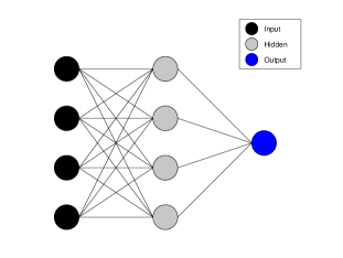
Figure 1: An architecture of a fully-connected neural network.

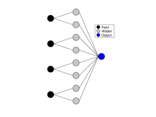
Figure 2: An architecture for a neural additive model. Each feature does not interact with each other.

III Generalized gloves of neural additive models

We intend to develop machine learning models based on the additive form which have the simplest architecture and highest accuracy (SHA). We will first separate linear and nonlinear components using the forward stepwise selection algorithm. We then propose generalized sparse neural additive models to further sparsify nonlinear structures with the method to identify statistical interactions.

III-A Forward stepwise selection

We now show how to separate linear and nonlinear components. Suppose the input $\mathbf{x}$ with the feature index $D=\{1,\dots,p\}$ can be split into linear components $\mathbf{x}_{U}$ and nonlinear components $\mathbf{x}_{V}$, where $U\cup V=D$ and $U\cap V=\emptyset$, then we assume $f$ takes the additive form of

$$g(\mathbb{E}[y|\mathbf{x}])=\alpha+\sum_{u:u\in U}\beta_{u}x_{u}+f_{V}(\mathbf{x}_{V}),$$ (4)

where $f_{V}$ is parametrized by a FCNN. In the case of $U=\emptyset$, $g$ reduces to a FCNN; in the case of $V=\emptyset$, $g$ reduces to a LaLR. An example of the architecture with two linear features and two nonlinear features is shown in Figure 3. The new architecture (4) improve NAMs by including linear components, and allowing complex interactions between nonlinear components, but at the expense of neglecting potential sparse additive forms in nonlinear components. This will be explored later on.

Consequently, we need an algorithm to distinguish between linear and nonlinear components. In our empirical experiments, we have found that in many datasets, only a few features exhibit nonlinear behaviors, suggesting that we could use a forward stepwise selection method to distinguish linear from nonlinear features. The procedure is summarized in Algorithm 1. A backward stepwise selection is certainly another option and will be similar. The worst case scenario of the forward selection algorithm requires $\frac{p(p-1)}{2}$ times of training. But, as we will see in empirical experiments, this could happen early. For problems with large $p$, it may be applied after feature selection. As the focus of this paper is not on general feature selection, we will not discuss further. However, we would like to highlight that a feature reduction can be effective, but neglects the fact that a feature can be both linear and important. As an example, the sales of a product are closely tied to the binary feature holiday, which is often represented in a linear fashion in NNs. In this instance, a linear component is crucial. Thus, selection algorithms may be able to exclude this component, as opposed to general selection methods. In addition, this algorithm can be used as a starting point for other interactions detection methods, such as [20, 28].

The forward selection algorithm provides an efficient method of distinguishing linear components from nonlinear ones. This method is helpful for reducing the dimensionality of nonlinear features and serves as an initialization method for more complicated models, as we will discuss below. We should clarify that (4) is a stage on the way from NAMs to GGNAMs, in order to demonstrate the process.

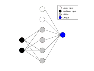
Figure 3: An architecture of (4). Nonlinear features have complex interactions.

Algorithm 1 Forward stepwise selection

1:  Inputs: $\epsilon>0$

2:  Train $f^{0}$ with loss $e^{0}$ by a LaLR

3:  Train $f^{p}$ with loss $e^{p}$ by a FCNN

4:  $i=1$

5:  $U=(1,\dots,p)$ and $V=\emptyset$

6:  while $e^{p}-e^{i}>\epsilon$ do

7:     for $u$ in $U$ do

8:        Train $f_{u}^{i}$ with loss $e^{i}_{u}$ using $U\setminus u$ and $V\cup u$

9:     end for

10:     $m=\text{argmin}_{u:u\in U}e^{i}_{u}$

11:     $U=U\setminus m$

12:     $V=V\cup m$

13:     $e^{i}=e^{i}_{m}$

14:     $f^{i}=f^{i}_{m}$

15:     $i=i+1$

16:  end while

17:  Output: $f^{i-1}$

III-B Generalized gloves of neural additive model

We present generalized gloves of neural additive models (GGNAMs), which further sparsify nonlinear interactions in (4). Features are divided into two categories:

• Linear component $\mathbf{x}_{U}$, similar to (4).

• Nonlinear component $\mathbf{x}_{V}$: subsets $v\in V$ are allowed to be either a single element or multiple elements that allow interactions.

Consequently, there are three types of features: linear features, individual nonlinear features, and interacted nonlinear features. It is worth emphasizing that GGNAMs allow different interactions groups to avoid global interactions. Different from (3) and (4), GGNAMs have the following form:

$$g(\mathbb{E}[y|\mathbf{x}])=\alpha+\sum_{u:u\in U}\beta_{u}x_{u}+\sum_{v:v\in V}f_{v}(\mathbf{x}_{v}).$$ (5)

As an simple example, we can have

$$g(\mathbb{E}[y|\mathbf{x}])=\alpha+\beta x_{1}+f_{1}(x_{2})+f_{2}(x_{3},x_{4}),$$

which is visualized in Figure 4. GGNAMs offer advantages over NAMs by allowing for linear components and complicated interactions.

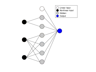
Figure 4: An architecture of the generalized gloves of neural additive model. It splits features into linear component, individual nonlinear component, and interacted nonlinear component.

III-C Identify statistical interactions

While GGNAMs have enabled flexible architectures that can take into account a variety of possibilities, we still require a convenient method for determining the architecture of GGNAMs. As a first step, we employ the forward selection algorithm 1 to reduce the dimensions of nonlinear features. Once linear features are determined, we can now investigate interactions among nonlinear features.

Statistical interactions have been studied extensive in the exist literature [25, 26, 27]. For simplicity, suppose there are two groups: $\mathbf{x}$ can be split into two components $\mathbf{x}_{U}$ and $\mathbf{x}_{V}$, with $U\cup V=D$ and $U\cap V=\emptyset$, where $D=\{1,\dots,p\}$. Extending it to multiple groups is straightforward. Our goal is to test whether a function is additively separable.

Definition 1.

We say a function $f$ with $D$ is strictly additive separable for $U$ and $V$ if

$$f(\mathbf{x})=g(\mathbf{x}_{U})+h(\mathbf{x}_{V})$$ (6)

for some functions $g$ and $h$, $U\cup V=D$, and $U\cap V=\emptyset$.

Our goal is to identify these two groups. Both groups have a variety of features and exhibit complex interrelationships, which presents a challenge. In order to simplify the procedure, we focus on pairwise features $x_{i}$ and $x_{j}$ and examine whether there are direct interactions between them. That is, without loss of generality, we wish to know if $x_{i}\in U$ and $x_{j}\in V$, where $U\cap V=\emptyset$. Unfortunately, $U$ and $V$ are unknown in advance. To avoid explicitly requiring information for $U$ and $V$, we generalize the idea to allow duplicates for both $U$ and $V$.

Definition 2.

We say a function $f$ with $D$ is additive separable for $U$ and $V$ if

$$f(\mathbf{x})=g(\mathbf{x}_{U})+h(\mathbf{x}_{V})$$ (7)

for some functions $g$ and $h$, $U\cup V=D$, and $U$ and $V$ are not necessarily disjoint.

Clearly, additive separability covers strictly additive separability. Without knowing $U$ and $V$, this generalization allows us to reconsider larger sets $D\setminus i$ and $D\setminus j$, which cover $U$ and $V$. In addition, the following theorem can be easily verified.

Theorem 1 (Additive Separability Theorem).

Suppose $f$ with $D$ can be split into two disjoint sets $U,V$ with $i\in U$ and $j\in V$, then $f$ is additive separable for $D\setminus i$ and $D\setminus j$ if and only if $f$ is strictly additive separable for $U$ and $V$.

Proof.

If $f$ is separable for $D\setminus i$ and $D\setminus j$, then exists functions $g$ and $h$ such that

$$f(\mathbf{x})=g(\mathbf{x}_{D\setminus i})+h(\mathbf{x}_{D\setminus j}).$$

But then $g$ is separable for $U\setminus i$ and $V$, and $h$ is separable for $U$ and $V\setminus j$. Therefore, we can write

$$f(\mathbf{x}) =g_{1}(\mathbf{x}_{U\setminus i})+g_{2}(\mathbf{x}_{V})+h_{1}(\mathbf{x}_{U})+h_{2}(\mathbf{x}_{V\setminus j})$$

$$=p(\mathbf{x}_{U})+q(\mathbf{x}_{V}),$$

for some functions $g_{1},g_{2},h_{1},h_{2},p,q$. Conversely, we have

$$f(\mathbf{x}) =p(\mathbf{x}_{U})+q(\mathbf{x}_{V})=p_{1}(\mathbf{x}_{U\cup V\setminus j})+q_{1}(\mathbf{x}_{U\setminus i\cup V})$$

$$=q_{1}(\mathbf{x}_{D\setminus i})+p_{1}(\mathbf{x}_{D\setminus j})$$

for some functions $p_{1}$ and $q_{1}$. ∎

We learn from Additive Separability Theorem 1 that in order to check the separability of $x_{i}$ and $x_{j}$, we do not necessarily need to consider specific $U$ and $V$. Therefore, we follow [25]’s approach and test directly between $\mathbf{x}_{D\setminus i}$ and $\mathbf{x}_{D\setminus j}$. NNs have the universal approximation theorem, which allows them to learn $f$ arbitrarily well under a general assumption, as well as $g$ and $h$ in the additive form $f=g+h$. It is, therefore, convenient to compare a FCNN to a GGNAM with two nonlinear groups $D\setminus i$ and $D\setminus j$. We did not allow duplicate features in subsets in our definition of (5) for better demonstration, however, we should note there is no problem with allowing duplicate features. Then, $x_{i}$ and $x_{j}$ can be separated if there is almost no difference in validation process, for example,

$$\mathbb{E}[|f(\mathbf{x})-g(\mathbf{x}_{D\setminus i})-h(\mathbf{x}_{D\setminus j})|]<\epsilon.$$ (8)

Note that this is only one example and other metrics are certainly acceptable. Motivated by this, suppose the model accuracy is denoted by acc($f$), we consider a separability matrix $\mathbf{A}$ s.t.

$$A_{i,j}=\begin{cases}\text{acc}(f(\mathbf{x})),&\ \text{if }i=j,\\ \text{acc}(g(\mathbf{x}_{D\setminus i})+h(\mathbf{x}_{D\setminus j})),&\ \text{if }i\neq j.\end{cases}$$ (9)

If $|A_{i,i}-A_{i,j}|<\epsilon$ for some small $\epsilon$, then we conclude that there is no interactions. $\mathbf{A}$ offers an intuitive understanding of the consequences arising from decoupling features. In selecting $\epsilon$, there is a trade-off between accuracy and interpretation, which should be determined by problems and users’ appetites. Different $\epsilon$ can be useful even for the same dataset for various purposes. When predicting housing prices, a private company might choose a very small $\epsilon$ to seek arbitrage opportunities, whereas a finance researcher might choose a large $\epsilon$ to improve explanation when studying market efficiency. After interactions have been identified, features are grouped together if they have direct interactions or indirect interactions through some intermediate features. The overall procedure can be outlined in Algorithm 2.

Algorithm 2 Train a GGNAM

1:  Inputs: $\epsilon>0$, $D=\{1,\dots,p\}$

2:  Train $f_{\text{LaLR}}$ by a LaLR

3:  Train $f_{\text{FCNN}}$ by a FCNN

4:  Perform forward selection algorithm 1 with $f_{\text{LaLR}}$ and $f_{\text{FCNN}}$ to split $D$ into linear component $U$ and nonlinear component $V$

5:  Calculate the separability matrix $\mathbf{A}$ by (9)

6:  Split $V$ into disjoint $v_{i}$ based on $\mathbf{A}$

7:  Train a $f_{\text{GGNAM}}$ with $U$ and $V$

8:  Output: $f_{\text{GGNAM}}$

We would like to explain why we selected this approach. There is a balance between robustness and efficiency. Derivative-based methods, such as [27], can be very efficient. In many applications, including image and texture data, it has proven to be successful. The individual testing may be slower, but it is potentially more robust as the separability is calculated exactly. In empirical results, an example is provided to illustrate a potential problem with the Hessian calculations. While the integration Hessian [29] could potentially avoid such issues, the choice of path is unclear in many datasets in finance as the data is structured. In finance, computational burden is typically less significant due to less amount of data and features. Particularly, the number of features in finance is generally small due to concerns about discrimination, bias, etc. Thus, we decide to perform individual testing for robustness.

IV Empirical examples

This section evaluates the performance of models for a variety of datasets, including two classification problems and one regression problem. Specifically, we compare linear and logistic regressions (LaLRs), fully-connected neural networks (FCNNs), neural additive models (NAMs), and generalized gloves of neural additive models (GGNAMs). We randomly split datasets into training ($80\%$) and testing ($20\%$). For hyperparameter tuning of separating linear and nonlinear features as well as interactions, a 20$\%$ hold-out validation set is further split from the training set. The area under the curve (AUC) is used to measure performance in classification because datasets are highly imbalanced; the root-mean-square-error (RMSE) is used in regression. Then, we provide a detailed post-analysis. For example, function behaviors associated with certain features are plotted and analyzed. In such cases, intercepts are subtracted as they are not relevant.

As part of the model architecture, we use the same structure for FCNNs and individual neural networks (NNs) in NAMs and GGNAMs so that they have the same number of parameters. For classification, NNs contain 1 hidden layer with 5 units, logistic activation, and no regulation. For regression, NNs contain 2 hidden layers with $[16,8]$ units, ReLU activation, and a l2 penalty is applied with $\lambda=2e^{-4}$. Since such simple architectures are compared favorably with results from the literature, we do not explore more complex ones. This is a clear indicator of the weak nonlinearity in datasets, which is the basis of our method’s success. We wish to emphasize that our study focuses on highly regulated financial industries, where both transparency and explainability are crucial. The use of very deep learning methods is usually not necessary in these datasets.

In this study, we have neglected other advanced ML methods, such as random forest (RF) and extreme gradient boosting (XGBoost). For some datasets, a comparison of FCNNs with these methods can be found in [22, 20]. Since our model is a simplified architecture of FCNNs, theoretically, its accuracy should not exceed FCNNs. Thus, for advanced black-box ML methods, we only include FCNNs in experiments for better demonstrations. We shall highlight that the focus of our method is on interpretation rather than accuracy: we are capable of providing exact explanations with the same level of accuracy as FCNNs.

IV-A Taiwan credit scoring data

IV-A1 Data description

Taiwan credit scoring dataset [30] is concerned with clients’ probability of default (PoD). Card-issuing banks over issued cash and credit cards to unqualified applicants, which led to high delinquencies for banks during this period. The study aimed to identify high risk clients based on their credit histories and to deny applications that were deemed unlikely to be repaid. In credit scoring, interpretation by regulators is strictly mandatory [7]: a detailed explanation must be given to customers upon denial. Please see [31] for a more detailed explanation of the requirements.

The data was collected from an important bank in Taiwan in October 2005. Of the total 30,000 observations, 6,639 (22.12$\%$) relate to cardholders with default payments. The response variable in this study is a binary variable, default payment. It contains 23 features as follows:

• $x_{1}$: Amount of the given credit (NT dollar): this includes both the individual consumer’s credit and his/her family (supplementary) credit.

• $x_{2}$: Gender (1 = male; 2 = female).

• $x_{3}$: Education (1 = graduate school; 2 = university; 3 = high school; 0,4,5,6 = others).

• $x_{4}$: Martial status (1 = married; 2 = single; 3 = divorce; 0 = others).

• $x_{5}$: Age (years).

• $x_{6}-x_{11}$: History of past payments. These variables track the past monthly payment records (from April to September, 2005) as follows: $x_{6}$= repayment status in September, 2005; $x_{7}$= the repayment status in August, 2005; …; $x_{11}$= repayment status in April, 2005. The measurement scale for the repayment status is $-2$= No consumption; $-1$= Paid in full; 0=The use of revolving credit; 1=Payment delay for one month; 2= Payment delay for two months; …; 8=Payment delay for eight months; 9= Payment delay for nine months and above.

• $x_{12}-x_{17}$: Amount of bill statement (NT dollar). $x_{12}$= Amount of bill statement in September, 2005; $x_{13}$=Amount of bill statement in August, 2005; …; $x_{17}$= Amount of bill statement in April, 2005.

• $x_{18}-x_{23}$: Amount of previous payment (NT dollar). $x_{18}$ = Amount paid in September, 2005; $x_{19}$ = Amount paid in August, 2005; $x_{23}$ = Amount paid in April, 2005.

• $y$: Client’s behavior; 0 = Not default; 1 = Default.

IV-A2 Results

A comparison of performance is presented in Table I. We begin by examining the results of the LaLR, FCNN, and NAM. The NAM performs similarly to the FCNN, and both methods outperform the LaLR, demonstrating the value of ML techniques. As the NAM has already attained the same accuracy as the FCNN, we do not expect any intersections to exist. We will confirm this later. The strength of the NAM is evident from this, and we find it somewhat surprising, as we would have expected greater interactions, for example, between periods of delinquency.

Then, we examine the results of the forward selection algorithm. Interesting to note is that of 23 features, only two are selected as nonlinear features, namely $x_{6}$ and $x_{1}$ in order. This significantly reduces the dimensionality of nonlinear features. Then, we calculate the separability matrix (9) based on AUC in Table II. It is evident that separating these features is not harmful. Accordingly, we confirm that there are no interactions. We then visualize selected nonlinear features in Figure 5. As the result of $x_{1}$ illustrates, clients with more given credits are likely to be more reliable, as banks would not extend credits if they did not trust them. The monotonic behavior of $x_{6}$ starting from 0, illustrates that with delayed payments, clients are more likely to default. Additionally, for these two features, nonlinearities can be summarized by diminishing marginal effects (DMEs). This means that additional changes will have a diminishing effect. As an example, the first delinquency will increase the client’s risk level significantly, while delinquencies of four or five times do not seem to matter very much. DMEs are commonly found in social science, and nonlinearity of this kind lead to the failure of the LaLR. The inability to capture DMEs in this case can be presented as the primary reason for the use of GGNAMs over LaLRs to regulators. In theory, we would expect DMEs to also apply for other features, including those related to delinquency. Nevertheless, there is insufficient evidence to determine their significance. Nonlinearities that are too weak to be detected should be ignored in favor of a simpler model of transparency. We would like to point out that such a visualization is easy by explainable ML methods, such as NAMs and GGNAMs, but is inapplicable to more complex ML methods, such as FCNNs. A summary of the architectures of all models is provided in Table III. The GGNAM achieved the simplest architecture with equal degree of accuracy in this dataset, therefore it should be preferred.

Methods	AUC
LaLR	$0.721$
FCNN	$0.759$
NAM	$0.759$
GGNAM	$0.766$

TABLE I: Model performance for the Taiwan credit scoring dataset.

Feature	$x_{1}$	$x_{6}$
$x_{1}$	$0.764$	$0.761$
$x_{6}$		$0.764$

TABLE II: Separability matrix of the GGNAM for the Taiwan credit scoring dataset.

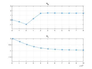
Figure 5: Output of the GGNAM with respect to $x_{1}$ and $x_{6}$ in the Taiwan credit scoring dataset. Diminishing marginal effects are observed for both features.

Model/Arch	Linear	Individual nonlinear	Nonlinear groups
LaLR	$x_{1}-x_{23}$
FCNN			$(x_{1},\dots,x_{23})$
NAM		$x_{1}-x_{23}$
GGNAM	$x_{2}-x_{5}$	$x_{1},x_{6}$
	$x_{7}-x_{23}$

TABLE III: Model architectures for the Taiwan credit scoring dataset.

IV-B Polish companies bankruptcy dataset

IV-B1 Data description

The dataset presented here represents predictions regarding bankruptcies of Polish companies [32]. There has always been an active field in business and economics dedicated to bankruptcy prediction [33], and its significance cannot be emphasized enough. The predictive power of such studies is important, but from a financial perspective it seems more important to understand their reasoning. The study of bankruptcy causes could potentially provide a wealth of information to regulators and policy makers.

Bankrupt companies were analyzed from 2000 to 2012, while still operating companies were evaluated from 2007 to 2013. The data contains financial rates from the first year of the forecasting period and a class label that indicates bankruptcy status after five years. It contains 7027 samples, in which 271 represent bankrupt companies. 64 indicators are used to represent the business conditions of companies, which is a common approach used in accounting research. It is noticeable that some indicators are highly correlated or contain overlapping information. In order to de-noise the data, we eliminate highly correlated ($>$0.95 or $<$-0.95) features and left with 34 features. We believe that this is a necessary practice for this study, as highly correlated features complicate interpretations of their effects. In addition, there are 5835 missing entries, which have been replaced by averaged feature values. Perhaps this is not the best method, and that could be improved by domain expertise. It is not, however, the main focus of the paper and we do not wish to complicate the discussion here.

• $x_{1}$: net profit / total assets

• $x_{2}$: total liabilities / total assets

• $x_{3}$: current assets / short-term liabilities

• $x_{4}$: [(cash + short-term securities + receivables - short-term liabilities) / (operating expenses - depreciation)] * 365

• $x_{5}$: retained earnings / total assets

• $x_{6}$: EBIT / total assets

• $x_{7}$: book value of equity / total liabilities

• $x_{8}$: sales / total assets

• $x_{9}$: equity / total assets

• $x_{10}$: gross profit / short-term liabilities

• $x_{11}$: (gross profit + depreciation) / sales

• $x_{12}$: (total liabilities * 365) / (gross profit + depreciation)

• $x_{13}$: (gross profit + depreciation) / total liabilities

• $x_{14}$: gross profit / sales

• $x_{15}$: sales (n) / sales (n-1)

• $x_{16}$: (equity - share capital) / total assets

• $x_{17}$: profit on operating activities / financial expenses

• $x_{18}$: working capital / fixed assets

• $x_{19}$: logarithm of total assets

• $x_{20}$: (current liabilities * 365) / cost of products sold

• $x_{21}$: operating expenses / short-term liabilities

• $x_{22}$: operating expenses / total liabilities

• $x_{23}$: profit on sales / total assets

• $x_{24}$: (current assets - inventories) / long-term liabilities

• $x_{25}$: total liabilities / ((profit on operating activities + depreciation) * (12/365))

• $x_{26}$: net profit / inventory

• $x_{27}$: (inventory * 365) / cost of products sold

• $x_{28}$: current assets / total liabilities

• $x_{29}$: (short-term liabilities * 365) / cost of products sold)

• $x_{30}$: equity / fixed assets

• $x_{31}$: working capital

• $x_{32}$: (current assets - inventory - short-term liabilities) / (sales - gross profit - depreciation)

• $x_{33}$: long-term liabilities / equity

• $x_{34}$: sales / receivables

• $y$: bankrupt or not

IV-B2 Results

We compare model performance in Table IV. Among the LaLR, FCNN, NAM, and GGNAM. Performance is ranked as FCNN$\approx$GGNAM$>$NAM$>$LR. Based on the results, it appears that ML methods are desirable for these datasets, and there are interactions that cannot be captured by the NAM.

Afterwards, we apply the forward stepwise selection algorithm to select nonlinear features starting from the LaLR. Surprisingly, out of 34 features, only three features, $x_{17}$, $x_{19}$, and $x_{22}$, are identified as nonlinear features, leading to a much smaller dimension which we didn’t foresee. The next step is to determine whether certain nonlinear features can be separated. According to the separability matrix in Table V, we conclude that only $x_{17}$ and $x_{22}$ definitely cannot be separated. We find this rather intriguing. The interaction among these features is to be expected; however, we did not anticipate an architecture that would be so sparse. The significance of these two features is not immediately apparent, among others. Nevertheless, if interactions are not necessary, then they should be omitted for transparency.

To verify whether such an interaction indeed exists, we calculate their joint marginal probability of bankruptcy (JMPoB) based on features $x_{17}$ and $x_{22}$ and record these results in a matrix, visualized in Figure 6. Both features are evenly divided into ten intervals, with approximately 700+ samples in each interval. Due to uneven distributions of features, we did not specify axes to facilitate better visualization. There are 100 boxes in total for two features with ten intervals each. In the absence of sufficient samples ($<30$) in the box, we denote the probability as $-0.1$, for purposes of visualization. It is evident that an abnormal pattern has been observed: for samples taken in the $10^{\text{th}}$ interval of $x_{17}$: the JMPoBs for small amounts of $x_{22}$ are exceptionally high. Patterns such as these are only found for large $x_{17}$, indicating that these features interact. The GGNAM allows us to demystify the black-box structure. In the following example, we calculate $f(x_{17},x_{22})$ at median values of samples within intervals of $x_{17}$ and $x_{22}$. Figure 7 demonstrates that the characteristics described above are somewhat reflected in this figure. The observed patterns suggest that in normal circumstances, a larger percentage of operating expenses over total liabilities increases the risk of bankruptcy. However, when a company makes significant profits from its operations over its financial expenses, a small percentage of operating expenses over total liabilities may be indicative of bankruptcy. This type of interaction has not yet been included in NAMs [22]. Visualizations like these should help us better comprehend the dataset and figure out the cause of the bankruptcy. Other patterns and approaches to visualization are certainly worthwhile to investigate; we merely present a simple example for illustration’s sake. It would also be very interesting to delve deeper into the analysis and understand the theory behind, with more bankruptcy datasets. This paper does not address such analyses because they would require an in-depth understanding of many business and economic theories.

Additionally, we show the potential problem of derivative calculation. We compute an integrated Hessian matrix $\mathbf{H}$ of the trained FCNN on the entire dataset, where

$$H_{i,j}=\sqrt{\sum_{k=1}^{n}\left(\frac{\partial^{2}f(\mathbf{x}_{k})}{\partial x_{i}\partial x_{j}}\right)^{2}},$$ (10)

and partial derivatives are simply computed through finite difference. As shown in Figure 8, $\mathbf{H}$ didn’t capture the interaction among $x_{17}$ and $x_{22}$ as it should have. This is because $x_{17}$ is highly unevenly distributed due to the ratio. While roughly $75\%$ of $x_{17}$ is less than 10, $\max x_{17}=2040800$. Therefore, it is perhaps inappropriate to treat the distance of $x_{17}$ equally. In light of such observations, we carefully identify model architectures by fitting models rather than by relying on derivatives.

Methods	AUC
LaLR	$0.677$
FCNN	$0.908$
NAM	$0.885$
GGNAM	0.907

TABLE IV: Model performance for the bankruptcy dataset.

Feature	$x_{17}$	$x_{19}$	$x_{22}$
$x_{17}$	0.913	0.908	0.881
$x_{19}$		0.913	0.910
$x_{22}$			0.913

TABLE V: Separability matrix of the GGNAM for the bankruptcy dataset

Model/Arch	Linear	Individual nonlinear	Nonlinear groups
LaLR	$x_{1}-x_{34}$
FCNN			$(x_{1},\dots,x_{34})$
NAM		$x_{1}-x_{34}$
GGNAM	$x_{1}-x_{16}$	$x_{19}$	$(x_{17},x_{22})$
	$x_{18}$
	$x_{20}-x_{21}$
	$x_{23}-x_{34}$

TABLE VI: Model architectures for the bankruptcy dataset.

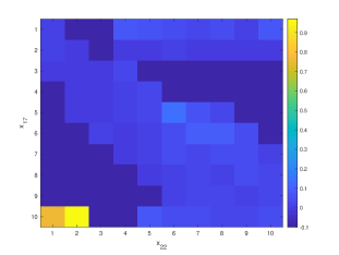
Figure 6: Joint marginal probabilities of bankruptcy for the features $x_{17}$ and $x_{22}$ for the bankruptcy dataset. In the $10^{\text{th}}$ interval of $x_{17}$, probabilities are exceptionally high in $1^{\text{th}}$ and $2^{\text{th}}$ interval of $x_{22}$.

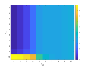
Figure 7: Output of the GGNAM with respect to $x_{17}$ and $x_{22}$ in the bankrupt dataset. The output is monotonically increasing with respect to $x_{22}$ in $1^{\text{th}}-9^{\text{th}}$ intervals of $x_{17}$, but is monotonically decreasing in $10^{\text{th}}$ interval of $x_{17}$.

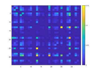
Figure 8: Integrated Hessian matrix (10) of the trained FCNN in the bankruptcy dataset. The interaction between $x_{17}$ is $x_{22}$ is unnoticeable.

IV-C Productivity prediction of garment employees dataset

IV-C1 Data description

This dataset aims to predict the productivity of garment workers [34, 35]. The specific objective of the study was to determine if there was a discrepancy between the targeted productivity set by authorities and the actual productivity in order to minimize potential losses. In spite of the objective to focus on the predictive power, it is important to keep in mind the possible ethnic and legal implications. Consider the following example: If a ML method predicts working overtime will enhance productivity, it would be unwise to recommend authorities increasing overtime. To better understand features with sensitive information, such as overtime, a transparent model would be desirable.

Detailed data were collected from the industrial engineering department of a garment manufacturing facility of a reputed company in Bangladesh. This dataset contains the production data for the sewing and finishing department for three months between January 2015 and March 2015. The dataset consists of 1197 samples and includes 14 features. We neglect the date feature and summarize the rest of features as follows:

• $x_{1}$: Quarters, from 1 to 5

• $x_{2}$: Associated department with the instance

• $x_{3}$: Days of the week

• $x_{4}$: Associated team number with the instance

• $x_{5}$: Targeted productivity set by the authority for each team for each day

• $x_{6}$: Standard Minute Value, it is the allocated time for a task

• $x_{7}$: Work in progress. Includes the number of unfinished items for products

• $x_{8}$: Represents the amount of overtime by each team in minutes

• $x_{9}$: Represents the amount of financial incentive (in BDT) that enables or motivates a particular course of action

• $x_{10}$: The amount of time when the production was interrupted due to several reasons

• $x_{11}$: The number of workers who were idle due to production interruption

• $x_{12}$: Number of changes in the style of a particular product

• $x_{13}$: Number of workers in each team

• $y$: The actual productivity value between 0 to 1

There are 506 missing entries for $x_{6}$, and we replace them with average value as in the last example.

IV-C2 Results

Model performance is compared in Table VII. All of the ML methods outperform the LaLR, and there is little difference among them. Based on the forward selection algorithm, only $x_{9}$ is identified as the nonlinear feature, so there’s no need to check interactions. Figure  9 clearly demonstrates the DME of financial incentive. On the basis of the above observation, one might suggest providing financial incentives, but only within certain limits. As can be seen in Table VIII, the GGNAM simplifies the NAM further by only using one nonlinear feature.

Methods	RMSE
LaLR	$0.151$
FCNN	$0.142$
NAM	$0.140$
GGNAM	$0.141$

TABLE VII: Model performance for the garment dataset

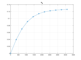
Figure 9: Output of the GGNAM with respect to $x_{9}$ in the garment dataset. The diminishing marginal effect is observed.

Model/Arch	Linear	Individual nonlinear	Nonlinear groups
LaLR	$x_{1}-x_{13}$
FCNN			$(x_{1},\dots,x_{13})$
NAM		$x_{1}-x_{13}$
GGNAM	$x_{1}-x_{8}$	$x_{9}$
	$x_{10}-x_{13}$

TABLE VIII: Model architectures for the garment dataset

V Conclusion

This paper introduces a novel class of generalized gloves of neural additive models (GGNAMs). In GGNAMs, features are categorized into three groups: linear features, individually nonlinear features, and features that interact. When features interact, they only interact with features within the same subset. In other words, interactions occur locally. We propose a stepwise selection method of distinguishing linear components from nonlinear components, and we carefully separate interacted groups based on additive separability criteria. Compared with recently introduced popular neural additive models (NAMs), GGNAMs support linear structures and highly complex high-order interactions. A linear structure provides greater transparency and is more favored by companies, while complex interactions ensure accuracy is not lost. Our extensive empirical studies have demonstrated the effectiveness of GGNAMs. In many finance datasets, linear features are predominant, individually nonlinear features are less common, and nonlinear interactions are comparatively rare. Using GGNAMs, these patterns can be captured with the simplest architecture and highest degree of accuracy, thereby providing an explanation-free machine learning method that is highly accurate.

A future extension of GGNAMs is possible. As an example, algorithmic fairness must be considered in the highly regulated financial sector. It can be accomplished by introducing constraints into the model. The extension and application of GGNAMs to more complex tasks, with more comprehensive explanations, is another promising area for future research. Due to the page limitations, we have not included more comprehensive explanations and more examples in the paper. Because explanations for different problems may vary, accuracy comparisons are inadequate, and therefore results cannot be summarised in a simple way. For example, when it comes to credit scoring, global explanations, local feature-based explanations, and local instance-based explanations may all be required. Research in these areas will be reported in the future.

References

- [1] A. Radford, J. Wu, R. Child, D. Luan, D. Amodei, I. Sutskever et al., “Language models are unsupervised multitask learners,” OpenAI blog, vol. 1, no. 8, p. 9, 2019.
- [2] K. He, X. Zhang, S. Ren, and J. Sun, “Deep residual learning for image recognition,” in Proceedings of the IEEE conference on computer vision and pattern recognition, 2016, pp. 770–778.
- [3] T. Chen and C. Guestrin, “Xgboost: A scalable tree boosting system,” in Proceedings of the 22nd acm sigkdd international conference on knowledge discovery and data mining, 2016, pp. 785–794.
- [4] “Are gans created equal? a large-scale study,” 2021.
- [5] C. d. Carlo, M. D. Bondt, and T. Evgeniou, “Ai regulation is coming,” Harvard Business Review, 2021. [Online]. Available: https://hbr.org/2021/09/ai-regulation- is- coming.
- [6] (2021) Model risk management. [Online]. Available: https://www.occ.treas.gov/publications-and-resources/publications/comptrollers-handbook/files/model-risk-management/index-model-risk-management.html
- [7] (2021) Cfpb acts to protect the public from black-box credit models using complex algorithms. [Online]. Available: https://www.consumerfinance.gov/about-us/newsroom/cfpb-acts-to-protect-the-public-from-black-box-credit-models-using-complex-algorithms/
- [8] J. Chen and V. Storchan, “Seven challenges for harmonizing explainability requirements,” arXiv preprint arXiv:2108.05390, 2021.
- [9] A. Sudjianto and A. Zhang, “Designing inherently interpretable machine learning models,” arXiv preprint arXiv:2111.01743, 2021.
- [10] Z. Yang, A. Zhang, and A. Sudjianto, “Enhancing explainability of neural networks through architecture constraints,” IEEE Transactions on Neural Networks and Learning Systems, vol. 32, no. 6, pp. 2610–2621, 2020.
- [11] C. Rudin, “Stop explaining black box machine learning models for high stakes decisions and use interpretable models instead,” Nature Machine Intelligence, vol. 1, no. 5, pp. 206–215, 2019.
- [12] T. Wang, C. Rudin, F. Doshi-Velez, Y. Liu, E. Klampfl, and P. MacNeille, “A bayesian framework for learning rule sets for interpretable classification,” The Journal of Machine Learning Research, vol. 18, no. 1, pp. 2357–2393, 2017.
- [13] M. T. Ribeiro, S. Singh, and C. Guestrin, ““why should i trust you?” explaining the predictions of any classifier,” in Proceedings of the 22nd ACM SIGKDD international conference on knowledge discovery and data mining, 2016, pp. 1135–1144.
- [14] S. M. Lundberg and S.-I. Lee, “A unified approach to interpreting model predictions,” Advances in neural information processing systems, vol. 30, 2017.
- [15] E. Horel, V. Mison, T. Xiong, K. Giesecke, and L. Mangu, “Sensitivity based neural networks explanations,” arXiv preprint arXiv:1812.01029, 2018.
- [16] E. Horel and K. Giesecke, “Significance tests for neural networks,” Journal of Machine Learning Research, vol. 21, no. 227, pp. 1–29, 2020.
- [17] C. Molnar, G. König, J. Herbinger, T. Freiesleben, S. Dandl, C. A. Scholbeck, G. Casalicchio, M. Grosse-Wentrup, and B. Bischl, “Pitfalls to avoid when interpreting machine learning models,” 2020.
- [18] I. E. Kumar, S. Venkatasubramanian, C. Scheidegger, and S. Friedler, “Problems with shapley-value-based explanations as feature importance measures,” in International Conference on Machine Learning. PMLR, 2020, pp. 5491–5500.
- [19] D. Slack, S. Hilgard, E. Jia, S. Singh, and H. Lakkaraju, “Fooling lime and shap: Adversarial attacks on post hoc explanation methods,” in Proceedings of the AAAI/ACM Conference on AI, Ethics, and Society, 2020, pp. 180–186.
- [20] Z. Yang, A. Zhang, and A. Sudjianto, “Gami-net: An explainable neural network based on generalized additive models with structured interactions,” Pattern Recognition, vol. 120, p. 108192, 2021.
- [21] C. Chen, K. Lin, C. Rudin, Y. Shaposhnik, S. Wang, and T. Wang, “An interpretable model with globally consistent explanations for credit risk,” arXiv preprint arXiv:1811.12615, 2018.
- [22] R. Agarwal, L. Melnick, N. Frosst, X. Zhang, B. Lengerich, R. Caruana, and G. E. Hinton, “Neural additive models: Interpretable machine learning with neural nets,” Advances in Neural Information Processing Systems, vol. 34, 2021.
- [23] E. Dumitrescu, S. Hue, C. Hurlin, and S. Tokpavi, “Machine learning for credit scoring: Improving logistic regression with non-linear decision-tree effects,” European Journal of Operational Research, vol. 297, no. 3, pp. 1178–1192, 2022.
- [24] P. Quell, A. Bellotti, J. Breeden, and J. Martin, “Machine learning and model risk management,” 2021. [Online]. Available: https://mrmia.org/white-papers/
- [25] D. Sorokina, R. Caruana, M. Riedewald, and D. Fink, “Detecting statistical interactions with additive groves of trees,” in Proceedings of the 25th international conference on Machine learning, 2008, pp. 1000–1007.
- [26] M. Tsang, H. Liu, S. Purushotham, P. Murali, and Y. Liu, “Neural interaction transparency (nit): Disentangling learned interactions for improved interpretability,” Advances in Neural Information Processing Systems, vol. 31, 2018.
- [27] M. Tsang, S. Rambhatla, and Y. Liu, “How does this interaction affect me? interpretable attribution for feature interactions,” Advances in neural information processing systems, vol. 33, pp. 6147–6159, 2020.
- [28] Y. Lou, R. Caruana, J. Gehrke, and G. Hooker, “Accurate intelligible models with pairwise interactions,” in Proceedings of the 19th ACM SIGKDD international conference on Knowledge discovery and data mining, 2013, pp. 623–631.
- [29] J. D. Janizek, P. Sturmfels, and S.-I. Lee, “Explaining explanations: Axiomatic feature interactions for deep networks,” Journal of Machine Learning Research, vol. 22, no. 104, pp. 1–54, 2021.
- [30] I.-C. Yeh and C.-h. Lien, “The comparisons of data mining techniques for the predictive accuracy of probability of default of credit card clients,” Expert Systems with Applications, vol. 36, no. 2, pp. 2473–2480, 2009.
- [31] A. B. Arrietaa, N. Dıaz-Rodrıguezb, J. Del Sera, A. Bennetotb, S. Tabikg, A. Barbadoh, S. Garciag, S. Gil-Lopeza, D. Molinag, R. Benjaminsh et al., “Explainable artificial intelligence (xai): concepts, taxonomies, opportunities and challenges toward responsible ai,” arXiv preprint arXiv:1910.10045, 2019.
- [32] M. Zieba, S. K. Tomczak, and J. M. Tomczak, “Ensemble boosted trees with synthetic features generation in application to bankruptcy prediction,” Expert systems with applications, vol. 58, pp. 93–101, 2016.
- [33] M.-Y. L. Li and P. Miu, “A hybrid bankruptcy prediction model with dynamic loadings on accounting-ratio-based and market-based information: A binary quantile regression approach,” Journal of Empirical Finance, vol. 17, no. 4, pp. 818–833, 2010.
- [34] A. Al Imran, M. N. Amin, M. R. I. Rifat, and S. Mehreen, “Deep neural network approach for predicting the productivity of garment employees,” in 2019 6th International Conference on Control, Decision and Information Technologies (CoDIT). IEEE, 2019, pp. 1402–1407.
- [35] A. A. Imran, M. S. Rahim, and T. Ahmed, “Mining the productivity data of the garment industry,” International Journal of Business Intelligence and Data Mining, vol. 19, no. 3, pp. 319–342, 2021.