Off-Policy Evaluation for Episodic Partially Observable Markov Decision Processes under Non-Parametric Models

Abstract

We study the problem of off-policy evaluation (OPE) for episodic Partially Observable Markov Decision Processes (POMDPs) with continuous states. Motivated by the recently proposed proximal causal inference framework, we develop a non-parametric identification result for estimating the policy value via a sequence of so-called V-bridge functions with the help of time-dependent proxy variables. We then develop a fitted-Q-evaluation-type algorithm to estimate V-bridge functions recursively, where a non-parametric instrumental variable (NPIV) problem is solved at each step. By analyzing this challenging sequential NPIV problem, we establish the finite-sample error bounds for estimating the V-bridge functions and accordingly that for evaluating the policy value, in terms of the sample size, length of horizon and so-called (local) measure of ill-posedness at each step. To the best of our knowledge, this is the first finite-sample error bound for OPE in POMDPs under non-parametric models.

1 Introduction

In practical reinforcement learning (RL), a representation of the full state which makes the system Markovian and therefore amenable to most existing RL algorithms is not known a priori. Decision makers are often facing so-called partial observability of the state information, which significantly hinders the task of RL. In general, agents have to maintain all historical information and establish a belief system on the hidden state for optimal decision making. A partially observable Markov decision process (POMDP) is often used to model the data generating process. See examples in robotics (Rafferty et al., 2011), precision medicine (Tsoukalas et al., 2015), stochastic game (Hansen et al., 2004) and many others. However, it is well known that learning optimal policies in POMDP is computationally intractable (Papadimitriou and Tsitsiklis, 1987). The issue of partial observability becomes more serious in the batch setting, where agents are not able to actively collect additional data and further explore the environment. For example, standard off-policy evaluation (OPE) methods, which aim to learn a policy value from the batch data generated from some behavior policy, would fail to give a consistent estimate because of unobserved state variables.

Due to this practical concern, there is a recent line of research studying the OPE under the framework of a confounded POMDP, where the behavior policy to generate the batch data is allowed to depend on some unobserved state variables (e.g., Tennenholtz et al., 2020; Nair and Jiang, 2021; Bennett and Kallus, 2021; Shi et al., 2021). Their identification results on the policy value are inspired by the negative controls or so-called proxy variables in the literature of causal inference (e.g., Miao et al., 2018a; Tchetgen Tchetgen et al., 2020). A building block of these results is the existence of some bridge functions, namely $Q$/$V$-bridge or weight-bridge functions, which are projections of the $Q$/$V$-functions or importance weights defined over the original state space onto the observation space. The corresponding statistical estimation of these bridge functions mainly relies on solving linear integral equations (e.g., Kress, 1989). Different from the tabular case studied by Tennenholtz et al. (2020) and Nair and Jiang (2021) and linear models studied by Shi et al. (2021) theoretically, solving linear integral equations with non-parametric models in the continuous state/observation space are known to be challenging due to the potential ill-posedness (Chen and Reiss, 2011), leading to slow statistical convergence rates. However, existing theoretical results developed by Bennett and Kallus (2021) and Shi et al. (2021) require fast enough convergence rates for these bridge function estimators in order to establish the asymptotic normality of their estimators for OPE, which could be illusive when the problem is seriously ill-posed under non-parametric models. This is different from the supervised learning where a fast enough convergence rate can be easily achieved under non-parametric models. Therefore, to fill this important theoretical gap, it is necessary to study the finite-sample performance of OPE of which bridge functions are estimated non-parametrically.

Motivated by these, in this paper, we study the OPE for confounded and episodic POMDPs with continuous states, where we non-parametrically estimate $V$-bridge functions. Our main contribution to the literature is three-fold. First, relying on some time-dependent proxy variables, we establish a non-parametric identification result for OPE using $V$-bridge functions for time-inhomogeneous confounded POMDPs. Based on the identification result, we develop a new fitted-Q-evaluation(FQE)-type approach to estimating $V$-bridge functions recursively and obtain an estimator for OPE based on the bridge function estimators. At each step of our algorithm, we propose to fit a non-parametric instrumental variable (NPIV) regression using a min-max estimation method, i.e., solving a linear integral equation with a non-parametric model. Our algorithm can be viewed as a sequential NPIV estimation, which is not well studied in the literature. Second and most importantly, we establish the finite-sample error bound for estimating $V$-bridge functions and accordingly that for evaluating the policy value, in terms of the sample size, length of horizon and (local) measure of ill-posedness at each step. Unlike the well studied standard NPIV model in the econometrics literature (e.g., Ai and Chen, 2003; Newey and Powell, 2003) where the response variable is directly observed, the response variable in our NPIV model at each step of the algorithm relies on the model estimate at its previous step. This difference makes our theoretical analysis substantially difficult. By carefully characterizing the statistical error due to the NPIV estimation at each step and more importantly, its propagation effect on future estimates, we are able to establish the first finite-sample result of OPE for confounded POMDPs under non-parametric models, which achieves a polynomial order over the length of horizon and sample size. Finally, our theoretical results on the sequential NPIV estimation are generally applicable to other sequential-type conditional moment restriction problems. The development of the uniform finite-sample error bounds of the NPIV estimation, extending the pointwise result in the previous literature such as Dikkala et al. (2020), may be of independent interest.

2 Related Work

Recently there is a surge of interest in studying OPE with unobserved variables in the sequential decision making problem. Specifically, Zhang and Bareinboim (2016) are among the first who proposed the framework of confounded MDPs, which essentially considers i.i.d. confounders in the dynamic system and therefore preserves the Markovian property. Along this direction, OPE methods are developed under various identification conditions such as partial identification using sensitivity analysis (Namkoong et al., 2020; Kallus and Zhou, 2020; Bruns-Smith, 2021), instrumental variable or mediator assisted OPE (Liao et al., 2021; Li et al., 2021; Shi et al., 2022) and many others. Another line of research focuses on more general confounded POMDP models , where the Markovian assumption is violated, under which several point estimation results were developed such as the aforementioned proxy variables related methods (Tennenholtz et al., 2020; Deaner, 2018; Ying et al., 2021; Bennett and Kallus, 2021; Nair and Jiang, 2021; Shi et al., 2021), spectral methods in undercomplete POMDPs (Hsu et al., 2012; Anandkumar et al., 2014; Jin et al., 2020) and predictive state representation related methods (Littman and Sutton, 2001; Singh et al., 2012; Cai et al., 2022).

Our proposed method, which uses proxy variables for OPE, is closely related to those recently developed by Bennett and Kallus (2021), Shi et al. (2021), and Ying et al. (2021). Bennett and Kallus (2021) and Ying et al. (2021) studied episodic POMDPs (or complex longitudinal studies) and mainly focused on developing asymptotic normality results of their policy value estimators. Their results rely on some high level rate conditions on the bridge function estimation, which are unknown if they would be satisfied when using non-parametric models due to the aforementioned measure of ill-posedness. Shi et al. (2021) mainly focused on time-homogeneous infinite-horizon POMDPs and developed asymptotic normality for their estimators under similar high-level conditions, which therefore has the same issue. Besides, while Shi et al. (2021) also established finite-sample bounds for their bridge function estimation and corresponding OPE, they only study the tabular case or linear/parametric models, where the issue of ill-posedness does not exist. In this paper, we provide a systematic investigation on the estimation of $V$-bridge functions and establish finite-sample guarantees for them and the corresponding OPE under non-parametric models. Specifically, we tackle the challenging episodic setting, where $V$-bridge functions are estimated sequentially. Without carefully controlling the effect of ill-posedness at each step and its propagation effect on future steps, the estimation error for these $V$-bridge functions and also that for OPE could be exponentially large in terms of the length of horizon. Motivated by the chaining argument in the empirical process theory, we successfully disentangle the effects of ill-posedness on the current step and future steps separately and thus establish finite-sample bounds for $V$-bridge functions and OPE both with a polynomial dependence on the length of horizon, which are new theoretical results we contribute to the literature.

Since our $V$-bridge function estimation can be formulated as a sequential NPIV problem, it is natually related to classical NPIV estimations, which have been extensively studied in the econometrics literature (see, e.g., Newey and Powell, 2003; Ai and Chen, 2003, 2012; Hall and Horowitz, 2005; Chen and Reiss, 2011; Chen and Christensen, 2018; Darolles et al., 2011; Blundell et al., 2007, for earlier reference). Recently there is also a growing interest in the min-max estimation for NPIV models (see, e.g., Muandet et al., 2020; Dikkala et al., 2020; Hartford et al., 2017, for some recent developments). As commented before, existing theoretical results for standard NPIV models cannot be directly applied to our setting due to the sequential structure of our FQE algorithm, so we need to develop new theory to address our setting. Technically, in order to establish a polynomial-order finite-sample error bound over the length of horizon for OPE, which is particularly important in RL, we decompose the measure of ill-posedness at each step of our sequential NPIV estimation into two components: the so-called (local) measure of one-step transition ill-posedness and the standard (local) measure of ill-posedness (e.g., Chen and Pouzo, 2012). Thanks to this novel decomposition, the effect of the first component on the estimation error of $V$-bridge functions and OPE is multiplicative but can be properly controlled while that of the second component could be large but is only cumulative. See Theorem 6.1. Finally, we remark that Ai and Chen (2012) also studied the sequential NPIV estimation problem, where the non-parametric components are estimated jointly. However, this method could be computationally inefficient in RL with a long horizon. More importantly, their results are built on the nested structure among conditional moment restriction models, which are not satisfied in our setting.

3 Preliminaries and Notations

In this section, we introduce the framework of discrete-time confounded POMDPs and its related OPE problem. Consider an episodic and confounded POMDP denoted by ${\cal M}=({\cal S},{\cal U},{\cal A},T,{\cal P},r)$, with ${\cal S}$ and ${\cal U}$ as the observed and unobserved continuous state spaces respectively, ${\cal A}$ as the discrete action space, $T$ as the length of horizon, ${\cal P}=\{\mathbb{P}_{t}\}_{t=1}^{T}$ as the transition kernel over ${\cal S}\times{\cal U}\times{\cal A}$ to ${\cal S}\times{\cal U}$, and $r=\{r_{t}\}_{t=1}^{T}$ as the reward function over ${\cal S}\times{\cal U}\times{\cal A}$. ${\cal S}$ can also be treated as the observation space in the classical POMDP. Then the process of ${\cal M}$ can be summarized as $\{S_{t},U_{t},A_{t},R_{t}\}_{t=1}^{T}$ with $S_{t}$ and $U_{t}$ as observed and unobserved state variables, $A_{t}$ as the action, and $R_{t}$ as the reward, where $r_{t}(s,u,a)={\mathbb{E}}[R_{t}\mid S_{t}=s,U_{t}=u,A_{t}=a]$ for any $(s,u,a)\in{\cal S}\times{\cal U}\times{\cal A}$. For simplicity, we assume that $|R_{t}|\leq 1$ uniformly in $1\leq t\leq T$.

The goal of OPE in a confounded POMDP is to evaluate the performance of a target policy using the batch data collected by some behavior policy. In this paper, the target policy we focus on is a sequence of functions mapping from the state space ${\cal S}$ to a probability mass function over the action space ${\cal A}$, denoted by $\pi=\{\pi_{t}\}_{t=1}^{T}$, where $\pi_{t}(a\mid s)$ is the probability of choosing an action $A_{t}=a$ given the state value $S_{t}=s$. We remark that our proposed identification results stated in Section 4 can be generalized to other policies such as history-dependent ones. Given a target policy $\pi$, define its state value function as

$$\textstyle V^{\pi}_{t}(s,u)={\mathbb{E}}^{\pi}[\sum_{t^{\prime}=t}^{T}R_{t^{\prime}}\mid S_{t}=s,U_{t}=u],\quad\text{for every $(s,u)\in{\cal S}\times{\cal U}$,}$$ (1)

where ${\mathbb{E}}^{\pi}$ denotes the expectation with respect to the distribution whose action at decision time $t$ follows $\pi_{t}$ for any $t\geq 1$. We consider the batch setting, where the observed action $A_{t}$ is generated by some behavior policy $\tilde{\pi}^{b}_{t}$ depending on both $S_{t}$ and $U_{t}$ for $1\leq t\leq T$. We aim to use the batch data to estimate the policy value of a target policy $\pi$, which is defined as

$${\cal V}(\pi)={\mathbb{E}}[V^{\pi}_{1}(S_{1},U_{1})],$$ (2)

where ${\mathbb{E}}$ denotes the expectation with respect to the behavior policy. Due to the unobserved $U_{t}$, standard OPE methods that rely on the Markovianity will give bias estimations. In the following, we introduce an identification result for estimating the policy value using some proxy variables.

Notations: For two sequences $\{\varpi(n)\}_{n\geq 1}$ and $\{\theta(n)\}_{n\geq 1}$, the notation $\varpi(n)\gtrsim\theta(n)$ (resp. $\varpi(n)\lesssim\theta(n)$) means that there exists a sufficiently large constant (resp. small) constant $c_{1}>0$ (resp. $c_{2}>0$) such that $\varpi(N)\geq c_{1}\theta(N)$ (resp. $\varpi(n)\leq c_{2}\theta(n)$). We use $\varpi(n)\asymp\theta(n)$ when $\varpi(n)\gtrsim\theta(n)$ and $\varpi(n)\lesssim\theta(n)$. For any random variable $X$, we use ${\mathcal{L}}^{q}\{X\}$ to denote the class of all measurable functions with finite $q$-th moments for $1\leq q\leq\infty$. Then the ${\mathcal{L}}^{q}$-norm is denoted by $\|\bullet\|_{{\mathcal{L}}^{q}\{X\}}$. When there is no confusion in the underlying distribution, we also write it as $\|\bullet\|_{{\mathcal{L}}^{q}}$ or $\|\bullet\|_{q}$. In particular, $\|\bullet\|_{\infty}$ denotes the sup-norm. In addition, we use Big $O$ and small $o$ as the convention.

4 Identification Results

Inspired by the proximal causal inference recently proposed by Tchetgen Tchetgen et al. (2020), we develop a non-parametric identification result for estimating ${\cal V}(\pi)$, which is similar to those by Bennett and Kallus (2021) and Shi et al. (2021). Assume that we can additionally observe the so-called reward-inducing proxy variables $W_{t}$ that are only related to the action $A_{t}$ through $(S_{t},U_{t})$ and action-inducing proxy variables $Z_{t}$ that are only related to the reward $R_{t}$ through $(S_{t},U_{t})$ at each decision time $t$. See Figure 1 for a directed acyclic graph (DAG) to illustrate their relationships and a time series data example in Miao et al. (2018b). For another example, the action-inducing proxy variables $Z_{t}$ can be defined as the observed history before time $t$, then $Z_{t}$ and related arrows in Figure 1 can be removed. Detailed assumptions and discussion are given in Appendix A. Denote the spaces of $\{Z_{t}\}_{t=1}^{T}$ and $\{W_{t}\}_{t=1}^{T}$ by ${\cal W}$ and ${\cal Z}$ respectively.

Figure 1: A representative DAG to illustrate the variables involved in the confounded POMDP.

Since the states $\left\{U_{t}\right\}_{t=1}^{T}$ are unmeasured, we cannot estimate the value function by the celebrated Bellman equation. However, with the help of confounding proxies $\left\{W_{t},Z_{t}\right\}_{t=1}^{T}$, the value of a target policy $\pi$ can be non-parametrically identified using observed variables under proper assumptions.

To proceed, we define a class of $V$-bridge functions (or $V$-bridges for short) $\{v^{\pi}_{t}\}_{t=1}^{T}$ defined over ${\cal W}\times{\cal S}$ such that for every $(s,u)\in{\cal S}\times{\cal U}$ and $t\geq 1$,

$$\textstyle{\mathbb{E}}\left[v^{\pi}_{t}(W_{t},S_{t})\mid U_{t}=u,S_{t}=s\right]={\mathbb{E}}^{\pi}\left[\sum_{t^{\prime}=t}^{T}R_{t^{\prime}}\,\Big{|}\,U_{t}=u,S_{t}=s\right].$$ (3)

If such $V$-bridges exist, then we obtain the following identification result for the policy value in (2).

Proposition 4.1 (Identification).

If there exist $\{v^{\pi}_{t}\}_{t=1}^{T}$ that satisfy (3), then the value of target policy $\pi$ can be identified by ${\mathcal{V}}(\pi)={\mathbb{E}}[v^{\pi}_{1}(W_{1},S_{1})].$

Note that $V$-bridges $\{v^{\pi}_{t}\}_{t=1}^{T}$ that satisfy (3) are not necessarily unique, but we can uniquely identify ${\mathcal{V}}(\pi)$ based on any of them. Next, we provide a theoretical guarantee for the existence of $V$-bridges $\{v^{\pi}_{t}\}_{t=1}^{T}$ in terms of a sequence of linear integral equations.

Theorem 4.1.

For a POMDP model of which variables satisfy the relationships illustrated in Figure 1 and some regularity conditions given in Appendix A, there always exist $V$-bridges $\{v^{\pi}_{t}\}_{t=1}^{T}$ satisfying (3). With $v^{\pi}_{T+1}=0$, a particular sequence of $V$-bridges $\{v^{\pi}_{t}\}_{t=1}^{T}$ can be obtained by solving the following linear integral equations:

$${\mathbb{E}}\left\{q^{\pi}_{t}(W_{t},S_{t},A_{t})-R_{t}-v^{\pi}_{t+1}(W_{t+1},S_{t+1})\mid Z_{t},S_{t},A_{t}\right\}=0,$$ (4)

where $\{q^{\pi}_{t}\}_{t=1}^{T}$ are $Q$-bridges defined over ${\cal W}\times{\cal S}\times{\cal A}$ such that

$$\textstyle{\mathbb{E}}\left[q^{\pi}_{t}(W_{t},S_{t},A_{t})\mid U_{t}=u,S_{t}=s,A_{t}=a\right]={\mathbb{E}}^{\pi}\left[\sum_{t^{\prime}=t}^{T}R_{t^{\prime}}\,\Big{|}\,U_{t}=u,S_{t}=s,A_{t}=a\right],$$ (5)

for every $(s,u,a)\in{\cal S}\times{\cal U}\times{\cal A}$ and $t\geq 1$, and $v^{\pi}_{t}(w,s)=\sum_{a\in{\mathcal{A}}}\pi_{t}(a\mid s)q^{\pi}_{t}(w,s,a)$. Clearly $Q$-bridges $\{q^{\pi}_{t}\}_{t=1}^{T}$ also exist.

Theorem 4.1 guarantees the existence of both $V$-bridges and $Q$-bridges, and also provides a natural procedure (4) to find $\{v^{\pi}_{t}\}_{t=1}^{T}$ and eventually estimate the policy value ${\cal V}(\pi)$. Then based on Proposition 4.1 and Theorem 4.1, we can perform OPE via Algorithm 1 in the population level. Specifically at each step we will solve (4) via a non-parametric model, which is a NPIV problem.

1 Input: $\{(S_{t},W_{t},Z_{t},A_{t},R_{t})\}_{t=1}^{T}$, a target policy $\pi=\{\pi_{t}\}_{t=1}^{T}$.

2 Let $v^{\pi}_{T+1}=0$.

3 Repeat for $t=T,\dots,1$:

4 Solve $v^{\pi}_{t}$ and $q^{\pi}_{t}$ by ${\mathbb{E}}\left\{q^{\pi}_{t}(W_{t},S_{t},A_{t})-R_{t}-v^{\pi}_{t+1}(W_{t+1},S_{t+1})\mid Z_{t},S_{t},A_{t}\right\}=0$ with $v^{\pi}_{t}(W_{t},S_{t})\triangleq\sum_{a\in{\mathcal{A}}}\pi_{t}(a\mid S_{t})q^{\pi}_{t}(W_{t},S_{t},a)$.

5

Output: ${\mathcal{V}}(\pi)={\mathbb{E}}[v^{\pi}_{1}(W_{1},S_{1})]$.

Algorithm 1 Identification of ${\mathcal{V}}(\pi)$

5 Estimation

In this section, we discuss how to estimate ${\cal V}(\pi)$ using batch data based on results given in Theorem 4.1 and Algorithm 1. Let a pre-collected training dataset be ${\cal D}_{n}=\{\left(S_{t,i},W_{t,i},Z_{t,i},A_{t,i},R_{t,i}\right)_{t=1}^{T}:i=1,\ldots,n\}$, which consists of $n$ i.i.d. copies of the observable trajectory $\left(S_{t},W_{t},Z_{t},A_{t},R_{t}\right)_{t=1}^{T}$ of a confounded POMDP. Following Algorithm 1, we develop a FQE-type approach where we propose to solve a min-max problem for estimating $v^{\pi}_{t}$ at the $t$-th step using the idea of Dikkala et al. (2020), and then apply Proposition 4.1 for OPE.

For convenience, we first rewrite the linear integral equations (4) for solving $V$-bridges in terms of operators. Define an operator $\widetilde{\mathcal{P}}_{t}:{\mathcal{L}}^{2}\{{\mathcal{R}}\times{\mathcal{W}}\times{\mathcal{S}}\}\rightarrow{\mathcal{L}}^{2}\{{\mathcal{Z}}\times{\mathcal{S}}\times{\mathcal{A}}\}$ such that $[\widetilde{\mathcal{P}}_{t}g](Z_{t},S_{t},A_{t})={\mathbb{E}}[g(R_{t},W_{t+1},S_{t+1})\mid Z_{t},S_{t},A_{t}]$ for any $g\in{\mathcal{L}}^{2}\{{\mathcal{R}}\times{\mathcal{W}}\times{\mathcal{S}}\}$. Define another operator $\overline{{\mathcal{P}}}_{t}:{\mathcal{L}}^{2}\{{\mathcal{W}}\times{\mathcal{S}}\times{\mathcal{A}}\}\rightarrow{\mathcal{L}}^{2}\{{\mathcal{Z}}\times{\mathcal{S}}\times{\mathcal{A}}\}$ such that for any $h\in{\mathcal{L}}^{2}\{{\mathcal{W}}\times{\mathcal{S}}\times{\mathcal{A}}\}$, $[\overline{{\mathcal{P}}_{t}}h](Z_{t},S_{t},A_{t})={\mathbb{E}}\left[h(W_{t},S_{t},A_{t})\mid Z_{t},S_{t},A_{t}\right].$ Motivated by (4), we define the V-bridge transition operator ${\mathcal{P}}^{\pi}_{t}:{\mathcal{L}}^{2}\{{\mathcal{R}}\times{\mathcal{W}}\times{\mathcal{S}}\}\rightarrow{\mathcal{L}}^{2}\{{\mathcal{W}}\times{\mathcal{S}}\}$ such that

$${\mathcal{P}}^{\pi}_{t}g=\left\langle\pi_{t},{\mathcal{P}}_{t}g\right\rangle,\ \text{ where ${\mathcal{P}}_{t}g=\overline{{\mathcal{P}}_{t}}^{-1}\widetilde{{\mathcal{P}}}_{t}g$ for all $g\in{\mathcal{L}}^{2}\{{\mathcal{R}}\times{\mathcal{W}}\times{\mathcal{S}}\}$.}$$

In particular, $\langle\pi_{t}(\cdot\mid S_{t}),[{\mathcal{P}}_{t}g](W_{t},S_{t},\cdot)\rangle\triangleq\sum_{a\in{\mathcal{A}}}\pi_{t}(a\mid S_{t})[{\mathcal{P}}_{t}g](W_{t},S_{t},a)$, and $\widetilde{\mathcal{P}}_{t}g$ is invertible by $\overline{{\mathcal{P}}_{t}}$. The invertibility is ensured by Assumption 8 in Appendix A.

Then by the definition of $V$-bridges and (4), we can identify $\{v^{\pi}_{t}\}_{t=1}^{T}$ via solving

$$v^{\pi}_{t}={\mathcal{P}}^{\pi}_{t}(v^{\pi}_{t+1}+R_{t}),\quad\text{for $t\geq 1$.}$$ (6)

To find the estimated V-bridges $\{\hat{v}^{\pi}_{t}\}_{t=1}^{T}$, it suffices to estimate ${\mathcal{P}}^{\pi}_{t}$. Note that one can regard (6) as a series of conditional moment model restrictions and we propose to solve them via a sequential NPIV estimation. In particular, at the $t$-th step, we adopt the min-max estimation method proposed by Dikkala et al. (2020) to estimate ${\mathcal{P}}^{\pi}_{t}$ non-parametrically as follows: $\widehat{{\mathcal{P}}}^{\pi}_{t}g=\left\langle\pi_{t},\widehat{{\mathcal{P}}}_{t}g\right\rangle$, where

$$\widehat{{\mathcal{P}}}_{t}g/(T-t+1)=\operatorname*{arg\,min}_{h\in{\mathcal{H}}^{(t)}}\Big{[}\sup_{f\in{\mathcal{F}}^{(t)}}\Big{\{}\Psi_{t,n}(h,f,g)-\lambda(\|f\|^{2}_{{\mathcal{F}}^{(t)}}+\frac{M}{\delta^{2}}\|f\|_{n}^{2})\Big{\}}+\lambda\mu\|h\|^{2}_{{\mathcal{H}}^{(t)}}\Big{]},$$ (7)

where $\|f\|_{n}^{2}=n^{-1}\sum_{i=1}^{n}f^{2}(Z_{t,i},S_{t,i},A_{t,i})$ for $f\in{\mathcal{F}}^{(t)}$. ${\mathcal{H}}^{(t)}$ on ${\mathcal{W}}\times{\mathcal{S}}\times{\mathcal{A}}$ and ${\mathcal{F}}^{(t)}$ on ${\mathcal{Z}}\times{\mathcal{S}}\times{\mathcal{A}}$ are two user-defined function spaces endowed with norms $\|\bullet\|_{{\mathcal{H}}^{(t)}}$ and $\|\bullet\|_{{\mathcal{F}}^{(t)}}$ respectively, $\lambda,\mu,M,\delta>0$ are tuning parameters, and

$$\Psi_{t,n}(h,f,g)=n^{-1}\textstyle\sum_{i=1}^{n}[h(W_{t,i},S_{t,i},A_{t,i})-(T-t+1)^{-1}g(R_{t,i},W_{t+1,i},S_{t+1,i})]f(Z_{t,i},S_{t,i},A_{t,i}),$$

where $g(R_{t},W_{t+1},S_{t+1})=R_{t}+\bar{g}(W_{t+1},S_{t+1})$ for some $\bar{g}\in{\mathcal{G}}^{(t+1)}$ on ${\mathcal{W}}\times{\mathcal{S}}$, endowed with norm $\|\bullet\|_{{\mathcal{G}}^{(t+1)}}$.

The rational behind (7) is that when $\lambda,\lambda\mu\rightarrow 0$ and $\lambda M/\delta^{2}\asymp 1$, the following two population-version min-max optimization problems

$$\min_{h\in{\mathcal{H}}^{(t)}}\sup_{f\in{\mathcal{F}}^{(t)}} {\mathbb{E}}[h(W_{t},S_{t},A_{t})-(T-t+1)^{-1}g(R_{t},W_{t+1},S_{t+1})]f(Z_{t},S_{t},A_{t})-\textstyle\frac{1}{2}f^{2}(Z_{t},S_{t},A_{t}),$$

$$\min_{h\in{\mathcal{H}}^{(t)}} {\mathbb{E}}\{{\mathbb{E}}[h(W_{t},S_{t},A_{t})-(T-t+1)^{-1}g(R_{t},W_{t+1},S_{t+1})\mid Z_{t},S_{t},A_{t}]\}^{2},$$

have the same solution $h$ when the space ${\mathcal{F}}^{(t)}$ of testing functions is rich enough. Note that $(T-t+1)^{-1}$ used above and in (7) are for scaling purpose.

After $T$ steps, we output our estimator for the policy value based on the empirical counterpart of Proposition 4.1. Our FQE-type algorithm is summarized in Algorithms 2 and 3 in Appendix E.

6 Theoretical Results

In this section, we establish the finite-sample bounds for the ${\mathcal{L}}^{2}$ error of estimating $V$-bridge $v^{\pi}_{1}$ and the error of OPE, in terms of the sample size, length of horizon and two (local) measures of ill-posedness. Our bounds also rely on the critical radii of certain spaces related to the user-defined function spaces ${\mathcal{H}}^{(t)}$ and ${\mathcal{F}}^{(t)}$ in (7), and also ${\mathcal{G}}^{(t)}$ of $V$-bridge functions.

1. Technical preliminaries. Before presenting our main results, we first introduce some concepts from the empirical process theory (Wainwright, 2019).

Definition 6.1 (Local Rademacher Complexity).

Given any real-valued function class ${\mathcal{F}}$ defined over a random vector $X$ and any radius $\delta>0$, the local Rademacher complexity is given by

$${\mathcal{R}}_{n}({\mathcal{F}},\delta)={\mathbb{E}}_{\epsilon,X}[\textstyle\sup_{f\in{\mathcal{F}}:\|f\|_{n}\leq\delta}|n^{-1}\textstyle\sum_{i=1}^{n}\epsilon_{i}f(X_{i})|],$$ (8)

where $\{X_{i}\}_{i=1}^{n}$ are i.i.d. copies of $X$ and $\left\{\epsilon_{i}\right\}_{i=1}^{n}$ are i.i.d. Rademacher random variables.

By bounding the local Rademacher complexity, which measures the complexity of the functional class ${\mathcal{F}}$ locally in a neighborhood of the ground truth, we can control the error rate of the proposed $V$-bridge estimator in each step. A crucial parameter for local Rademacher complexity of a function class ${\mathcal{F}}$ is called critical radius.

Definition 6.2 (Critical Radius).

Assume that ${\mathcal{F}}$ is a star-shaped function class, i.e. $\alpha f\in{\mathcal{F}}$ for any $f\in{\mathcal{F}}$ and scalar $\alpha\in[0,1]$, and also that ${\mathcal{F}}$ is $b$-uniformly bounded, i.e., $\|f\|_{\infty}\leq b<\infty$, $\forall f\in{\mathcal{F}}$. The critical radius of ${\mathcal{F}}$, denoted by $\delta_{n}$, is the solution to the inequality ${\mathcal{R}}_{n}({\mathcal{F}},\delta)\leq\delta^{2}/b.$

Additional Notations: We assume that the test functions $f$ belong to a star shaped, symmetric space ${\mathcal{F}}^{(t)}\subseteq{\mathcal{L}}^{2}({\mathcal{Z}}\times{\mathcal{S}}\times{\mathcal{A}})$ endowed with norm $\|\cdot\|_{{\mathcal{F}}^{(t)}}$. For brevity of notation, hereafter we suppress the time-step indicator $(t)$ in the context unless necessary. For a function space ${\mathcal{F}}$, we define $\alpha{\mathcal{F}}=\{\alpha f:f\in{\mathcal{F}}\}$, for some $\alpha\in{\mathbb{R}}$. Define ${\mathcal{F}}_{B}=\{f\in{\mathcal{F}}:\|f\|_{{\mathcal{F}}}^{2}\leq B\}$, for any $B>0$. Define the projected root mean squared error $\|\mbox{{\rm proj}}_{t}f\|_{2}=\sqrt{{\mathbb{E}}\{{\mathbb{E}}[f(X)\mid Z_{t},S_{t},A_{t}]\}^{2}}$, for any squared integrable $f$ with respect to the conditional distribution of $X$ given $(Z_{t},S_{t},A_{t})$.

Standard (Local) Measures of ill-posedness: Let $\bar{\tau}_{1}=\sup_{g\in{\mathcal{G}}^{(1)}}\|g(W_{1},S_{1})\|_{2}/\|{\mathbb{E}}[g(W_{1},S_{1})\mid Z_{1},S_{1}]\|_{2}$ be the measure of ill-posedness for ${\mathcal{G}}^{(1)}({\mathcal{W}}_{1}\times{\mathcal{S}}_{1})$ projected on ${\mathcal{Z}}_{1}\times{\mathcal{S}}_{1}$. Let $\tau_{t}=\sup_{h\in{\mathcal{H}}^{(t)}}\|h(W_{t},S_{t},A_{t})\|_{2}/\|\mbox{{\rm proj}}_{t}h(W_{t},S_{t},A_{t})\|_{2}$ be the standard measure of ill-posedness for ${\mathcal{H}}^{(t)}({\mathcal{W}}\times{\mathcal{S}}\times{\mathcal{A}})$ projected on ${\mathcal{Z}}\times{\mathcal{S}}\times{\mathcal{A}}$. It can be seen that $\bar{\tau}_{1},\tau_{t}\geq 1$ for $t\geq 1$. Indeed we only require measuring $\bar{\tau}_{1}$ and $\tau_{t}$ locally. See more details in Appendix C.

2. Results. We first give Assumption 1 used to develop our theoretical results below.

Assumption 1.

For each $t=1,\dots,T$,

1. Closeness. For any $g\in{\mathcal{G}}^{(t+1)}$, ${\mathcal{P}}_{t}(g+R_{t})\in{\mathcal{H}}^{(t)}$; For any $h\in{\mathcal{H}}^{(t)}$, $\left\langle\pi_{t},h\right\rangle\in{\mathcal{G}}^{(t)}$.

2. For any $h\in(T-t){\mathcal{H}}^{(t+1)}$, we have $\|{\mathcal{P}}_{t}\left(\frac{R_{t}+\left\langle\pi_{t+1},h\right\rangle}{T-t+1}\right)\|_{{\mathcal{H}}^{(t)}}^{2}\leq\|\frac{h}{T-t}\|_{{\mathcal{H}}^{(t+1)}}^{2}$.

3. There exists a constant $C_{{\mathcal{G}}}>0$ such that $\|\left\langle\pi_{t},h\right\rangle\|_{{\mathcal{G}}^{(t)}}^{2}\leq C_{{\mathcal{G}}}\|h\|_{{\mathcal{H}}^{(t)}}^{2}$, for $h\in{\mathcal{H}}^{(t)}$.

4. $q^{\pi}_{t}\in(T-t+1){\mathcal{H}}^{(t)}({\mathcal{W}},{\mathcal{S}},{\mathcal{A}})$ and $\|q^{\pi}_{T}\|_{{\mathcal{H}}^{(T)}}^{2}\leq M_{{\mathcal{H}}}$, where $M_{{\mathcal{H}}}>0$ is a constant.

5. Testing function class ${\mathcal{F}}^{(t)}$ is sufficiently rich such that there exists $L>0$, $\|f^{*}-\mbox{{\rm proj}}_{t}h_{t}\|_{2}\leq\eta_{n}^{(t)}$, where $f^{*}\in\operatorname*{arg\,min}_{f\in{\mathcal{F}}_{L^{2}\|h_{t}\|_{{\mathcal{H}}}^{2}}^{(t)}}\|f-\mbox{{\rm proj}}_{t}h_{t}\|_{2}$, for all $h_{t}\in{\mathcal{H}}^{(t)}$.

6. Behavior policies: there exists a constant $b_{\pi}$ such that $\pi_{t}^{b}(a\mid s)\triangleq{\mathbb{E}}[\tilde{\pi}_{t}^{b}(a\mid U_{t},S_{t})\mid S_{t}=s]\geq b_{\pi}>0$ for all $(s,a)\in{\cal S}\times{\cal A}$.

Assumption 1 (1) is similar to Bellman completeness, which has been widely used in RL without unobserved states (e.g., Antos et al., 2008). Note that both ${\mathcal{G}}^{(t)}$ and ${\mathcal{H}}^{(t)}$ can be chosen as infinite-dimensional spaces, e.g., RKHSs. Hence this assumption is relatively mild. Assumption 1 (2) requires the operator ${\mathcal{P}}_{t}$ to be bounded, which can be ensured under some continuity conditions on transition kernels (Kress, 1989). Assumption 1 (3) is a technical condition for controlling the complexity of ${\mathcal{G}}$ by ${\mathcal{H}}$. Assumption 1 (4) essentially assumes that we can model $q^{\pi}$ (and $v^{\pi}$) correctly at each $t$-step, which is again mild as ${\mathcal{H}}^{(t)}$ for $t\geq 1$ can all be chosen as infinite-dimensional spaces. This assumption is also called realizability of value functions, which is commonly seen in the literature of RL (e.g., Antos et al., 2008). Assumption 1 (5) is imposed to ensure that the space of testing functions ${\mathcal{F}}$ is large enough so that we are able to capture the conditional expectation operator in each min-max estimation (7). Assumption 1 (6) basically requires a full coverage of our batch data generating process induced by the behavior policy, which is widely used in OPE (Precup, 2000; Antos et al., 2008). Next, we provide a key decomposition of the ${\mathcal{L}}^{2}$ error for $V$-bridge estimation.

Theorem 6.1 (Error decomposition).

Under Assumption 1 (1) and (6), we can decompose the ${\mathcal{L}}^{2}$ error of the estimated $V$-bridge by

$$\|v^{\pi}_{1}-\hat{v}^{\pi}_{1}\|_{2}\leq\bar{\tau}_{1}\textstyle\sum_{t=1}^{T}\{\Pi_{t^{\prime}=1}^{t}C_{t^{\prime},t^{\prime}-1}^{(t)}\}\tau_{t}\|\pi_{t}/\pi_{t}^{b}\|_{\infty}\|\mbox{{\rm proj}}_{t}(\widehat{{\mathcal{P}}}_{t}-{\mathcal{P}}_{t})(\hat{v}^{\pi}_{t+1}+R_{t})\|_{2},$$

where the measures of one-step transition ill-posedness $C_{1,0}^{(t)}\triangleq 1$ and $C_{t^{\prime},t^{\prime}-1}^{(t)},2\leq t^{\prime}\leq t\leq T$ are defined after Corollary 6.2.

Theorem 6.1 shows that there are four key components for upper bounding the ${\mathcal{L}}^{2}$ error of $\hat{v}^{\pi}_{1}$. The first component is the probability ratio $\|\pi_{t}/\pi_{t}^{b}\|_{\infty}$, which is used to measure the distributional mismatch between the target and behavior policies. The second component is $\|\mbox{{\rm proj}}_{t}(\widehat{{\mathcal{P}}}_{t}-{\mathcal{P}}_{t})(\hat{v}^{\pi}_{t+1}+R_{t})\|_{2}$, the one-step projected error of $\widehat{{\mathcal{P}}}_{t}$ to ${\mathcal{P}}_{t}$, where $\hat{v}^{\pi}_{t+1}$ is the estimate for $v^{\pi}_{t+1}$ depending on the observed data after $t$-step. We remark that this is different from the analysis in the standard NPIV estimation with a directly measured outcome. Hence the results, e.g., from Dikkala et al. (2020), cannot be directly applied to bound this component. The last two components are related to the (local) measure of ill-posedness. The third component $\tau_{t}$ is the measure of ill-posedness for characterizing the difficulty of estimating $q^{\pi}_{t}$ by (4) using ${\mathcal{H}}^{(t)}$ at the $t$-th step. $\{\tau_{t}\}_{t=1}^{T}$ are similar to those used in the standard NPIV estimation such as Chen and Reiss (2011), and the effect of each $\tau_{t}$ on the upper bound is cumulative. The last component $\{\Pi_{t^{\prime}=1}^{t}C_{t^{\prime},t^{\prime}-1}^{(t)}\}_{t=1}^{T}$ quantify the propagation effect of estimation errors in previous steps on the last step of estimating $v^{\pi}_{1}$, which is multiplicative in terms of $C_{t^{\prime},t^{\prime}-1}^{(t)}$. We call $C_{t^{\prime},t^{\prime}-1}^{(t)}$ the measure of one-step transition ill-posedness from $t^{\prime}$ to $t^{\prime}-1$ related to $t$-step NPIV estimations. Next we provide detailed bounds for the second and last components. The discussion of the third component can be found in Appendix C.4.

Component 2: one-step projected error. In the following, we show that $\|\mbox{{\rm proj}}_{t}(\widehat{{\mathcal{P}}}_{t}-{\mathcal{P}}_{t})(\hat{v}^{\pi}_{t+1}+R_{t})\|_{2}$ is bounded by the critical radii of some spaces defined as balls ${\mathcal{H}}_{B}^{(t)}$, ${\mathcal{G}}_{C_{G}(T-t+1)M_{{\mathcal{H}}}}^{(t+1)}$ in hypothesis spaces ${\mathcal{H}}^{(t)}$, ${\mathcal{G}}^{(t+1)}$ respectively and a ball ${\mathcal{F}}_{3M}^{(t)}$ in testing space ${\mathcal{F}}^{(t)}$, for some fixed constants $M,B>0$ such that functions in ${\mathcal{H}}_{B}^{(t)}$ and ${\mathcal{F}}_{3M}^{(t)}$ have uniformly bounded ranges in $[-1,1]$ for all $1\leq t\leq T$. Let

$$\bm{\Omega}^{(t)} =\{(s_{t},w_{t},z_{t},a_{t},s_{t+1},w_{t+1})\mapsto r(h_{g}^{*}(w_{t},s_{t},a_{t})-g(w_{t+1},s_{t+1}))f(z_{t},s_{t},a_{t}):$$

$$\qquad g\in{\mathcal{G}}_{C_{G}(T-t+1)M_{{\mathcal{H}}}}^{(t+1)},f\in{\mathcal{F}}_{3M}^{(t)},r\in[0,1]\},\text{ and}$$

$$\bm{\Xi}^{(t)} =\{(s_{t},w_{t},z_{t},a_{t})\mapsto r[h-h_{g}^{*}](w_{t},s_{t},a_{t})f^{L^{2}B}(z_{t},s_{t},a_{t}):$$

$$\qquad h\in{\mathcal{H}}^{(t)},h-h_{g}^{*}\in{\mathcal{H}}_{B}^{(t)},g\in{\mathcal{G}}_{C_{G}(T-t+1)M_{{\mathcal{H}}}}^{(t+1)},r\in[0,1]\},$$

where $h_{g}^{*}\in{\mathcal{H}}^{(t)}$ is the solution to ${\mathbb{E}}\left[h(W_{t},S_{t},A_{t})-g(W_{t+1},S_{t+1})\mid Z_{t},S_{t},A_{t}\right]=0$, and $f^{L^{2}B}=\operatorname*{arg\,min}_{f\in{\mathcal{F}}_{L^{2}B}^{(t)}}\|f-\mbox{{\rm proj}}_{t}(h-h_{g}^{*})\|_{2}$ for a given $L>0$. An upper bound for $\|\mbox{{\rm proj}}_{t}(\widehat{{\mathcal{P}}}_{t}-{\mathcal{P}}_{t})(\hat{v}^{\pi}_{t+1}+R_{t})\|_{2}$ is given in Theorem 6.2.

Theorem 6.2.

Suppose that Assumption 1 holds. Let $\delta_{n}^{(t)}=\bar{\delta}_{n}^{(t)}+c_{0}\sqrt{\frac{\log(c_{1}T/\zeta)}{n}}$ for some universal constants $c_{0},c_{1}>0$ where $\bar{\delta}_{n}^{(t)}$ is the upper bound of the critical radii of ${\mathcal{F}}_{3M}^{(t)}$, $\bm{\Omega}^{(t)}$ and $\bm{\Xi}^{(t)}$. Assume that the approximation error in Assumption 1 (5) can be bounded by $\eta_{n}^{(t)}\leq\delta_{n}^{(t)}$. Furthermore, letting tuning parameters satisfy $M\lambda\asymp(\delta_{n}^{(t)})^{2}$ and $\mu\geq\mathop{}\mathopen{}\mathcal{O}\mathopen{}(L^{2}+M/B)$, with probability at least $1-\zeta$, we have

$$\|\mbox{{\rm proj}}_{t}(\widehat{{\mathcal{P}}}_{t}-{\mathcal{P}}_{t})(\hat{v}^{\pi}_{t+1}+R_{t})\|_{2}\lesssim M_{{\mathcal{H}}}(T-t+1)^{2}\delta_{n}^{(t)}\quad\text{for all $1\leq t\leq T$}.$$

Depending on the choices of ${\mathcal{H}}^{(t)}$, ${\mathcal{G}}^{(t+1)}$, and ${\mathcal{F}}^{(t)}$, we can obtain different finite-sample error bounds of the one-step projected error for each $t$. Below we provide two examples.

Corollary 6.1.

Let ${\mathcal{F}}^{(t)}$, ${\mathcal{H}}^{(t)}$ and ${\mathcal{G}}^{(t+1)}$ be VC-subgraph classes with VC dimensions ${\mathbb{V}}({\mathcal{F}}^{(t)})$, ${\mathbb{V}}({\mathcal{H}}^{(t)})$ and ${\mathbb{V}}({\mathcal{G}}^{(t+1)})$ respectively. Then with probability at least $1-\zeta$, for all $1\leq t\leq T$,

$$\|\mbox{{\rm proj}}_{t}(\widehat{{\mathcal{P}}}_{t}-{\mathcal{P}}_{t})(\hat{v}^{\pi}_{t+1}+R_{t})\|_{2}\lesssim(T-t+1)^{2.5}\textstyle\sqrt{\frac{\log(c_{1}T/\zeta)\max\{{\mathbb{V}}({\mathcal{F}}^{(t)}),{\mathbb{V}}({\mathcal{H}}^{(t)}),{\mathbb{V}}({\mathcal{G}}^{(t+1)})\}}{n}}.$$

The definition of the VC-subgraph class can be found in, e.g., Wainwright (2019). This is a broad class. For example, if one lets each of ${\mathcal{F}}^{(t)}$, ${\mathcal{H}}^{(t)}$ and ${\mathcal{G}}^{(t+1)}$ be a linear space ${\mathcal{F}}=\{\theta^{\top}\phi(\cdot):\theta\in{\mathbb{R}}^{d}\}$ with basis functions $\phi(\cdot)$, then ${\mathbb{V}}({\mathcal{F}})=d+1$. Then the upper bound for the one-step projected error becomes $\mathop{}\mathopen{}\mathcal{O}\mathopen{}((T-t+1)^{2.5}d/\sqrt{n})$.

Corollary 6.2.

Let ${\mathcal{H}}^{(t)}$, ${\mathcal{G}}^{(t+1)}$ and ${\mathcal{F}}^{(t)}$ be reproducing kernel Hilbert spaces (RKHSs) equipped with kernels $K_{{\mathcal{H}}^{(t)}}$, $K_{{\mathcal{G}}^{(t+1)}}$ and $K_{{\mathcal{F}}^{(t)}}$ respectively. For a given positive definite kernel $K$, we denote its nonincreasing eigenvalue sequence by $\{\lambda_{j}^{\downarrow}(K)\}_{j=1}^{\infty}$. We consider two scenarios for $\{\lambda_{j}^{\downarrow}(K)\}_{j=1}^{\infty}$.

(1) Polynomial eigen-decay: If $\lambda_{j}^{\downarrow}(K_{{\mathcal{H}}^{(t)}})\leq aj^{-2\alpha_{{\mathcal{H}}}}$, $\lambda_{j}^{\downarrow}(K_{{\mathcal{G}}^{(t+1)}})\leq aj^{-2\alpha_{{\mathcal{G}}}}$ and $\lambda_{j}^{\downarrow}(K_{{\mathcal{F}}^{(t)}})\leq aj^{-2\alpha_{{\mathcal{F}}}}$ for constants $\alpha_{{\mathcal{H}}},\alpha_{{\mathcal{G}}},\alpha_{{\mathcal{F}}}>1/2$ and $a>0$, then under the assumptions in Theorem 6.2, with probability at least $1-\zeta$, for all $1\leq t\leq T$, we have

$$\|\mbox{{\rm proj}}_{t}(\widehat{{\mathcal{P}}}_{t}-{\mathcal{P}}_{t})(\hat{v}^{\pi}_{t+1}+R_{t})\|_{2}\lesssim(T-t+1)^{2.5}\sqrt{\log(c_{1}T/\zeta)}n^{-\frac{1}{2+\max\{1/\alpha_{{\mathcal{H}}},1/\alpha_{{\mathcal{G}}},1/\alpha_{{\mathcal{F}}}\}}}\log(n).$$

(2) Exponential eigen-decay: If $\lambda_{j}^{\downarrow}(K_{{\mathcal{H}}^{(t)}})\leq a_{1}e^{-a_{2}j^{\beta_{{\mathcal{H}}}}}$, $\lambda_{j}^{\downarrow}(K_{{\mathcal{G}}^{(t+1)}})\leq a_{1}e^{-a_{2}j^{\beta_{{\mathcal{G}}}}}$ and $\lambda_{j}^{\downarrow}(K_{{\mathcal{F}}^{(t)}})\leq a_{1}e^{-a_{2}j^{\beta_{{\mathcal{F}}}}}$, for constants $a_{1},a_{2},\beta_{{\mathcal{H}}},\beta_{{\mathcal{G}}},\beta_{{\mathcal{F}}}>0$, then under the assumptions in Theorem 6.2, with probability at least $1-\zeta$, for all $1\leq t\leq T$, we have

$$\|\mbox{{\rm proj}}_{t}(\widehat{{\mathcal{P}}}_{t}-{\mathcal{P}}_{t})(\hat{v}^{\pi}_{t+1}+R_{t})\|_{2}\lesssim(T-t+1)^{2.5}\textstyle\left\{\sqrt{\frac{(\log n)^{1/\min\{\beta_{{\mathcal{H}}},\beta_{{\mathcal{G}}},\beta_{{\mathcal{F}}}\}}}{n}}+\sqrt{\frac{\log(c_{1}T/\zeta)}{n}}\right\}.$$

Kernels of the two types of eigen-decay considered above are very common. For example, the kernel of the $\alpha$-order Soblev space with $\alpha>1/2$, has a polynomial eigen-decay while the Gaussian kernel has an exponential eigen-decay, with $\beta=2$ for Lebesgue measure on real line and $\beta=1$ on a compact domain (Wei et al., 2017).

Components 4: measure of one-step transition ill-posedness. We first provide more insights on $\{\Pi_{t^{\prime}=1}^{t}C_{t^{\prime},t^{\prime}-1}^{(t)}\}_{t=1}^{T}$ before providing an upper bound. We formally define the local measure of one-step transition ill-posedness $C_{t^{\prime}+1,t^{\prime}}^{(t)}$ recursively based on $C_{t,t-1}^{(t)}$ to $C_{2,1}^{(t)}$ as

$$C_{t^{\prime}+1,t^{\prime}}^{(t)}\triangleq\sup_{g\in{\mathcal{G}}(W_{t^{\prime}+1}\times S_{t^{\prime}+1})}\frac{\|{\mathbb{E}}^{\pi_{t^{\prime}}}[g(W_{t^{\prime}+1},S_{t^{\prime}+1})\mid Z_{t^{\prime}},S_{t^{\prime}}]\|_{2}}{\|{\mathbb{E}}[g(W_{t^{\prime}+1},S_{t^{\prime}+1})\mid Z_{t^{\prime}+1},S_{t^{\prime}+1}]\|_{2}},\quad\text{subject to}$$

$$\|{\mathbb{E}}[g(W_{t^{\prime}+1},S_{t^{\prime}+1})\mid Z_{t^{\prime}+1},S_{t^{\prime}+1}]\|_{2}\lesssim\tau_{t}(T-t+1)^{2}\delta_{n}^{(t)}\|\pi_{t^{\prime}}/\pi_{t^{\prime}}^{b}\|_{\infty}\textstyle\prod_{s=t^{\prime}+1}^{t-1}C_{s+1,s}^{(t)},$$

with $C_{t+1,t}^{(t)}\triangleq 1$ for each $t=1,\dots,T$. For $C_{t,t-1}^{(t)}$, we can upper bound $\|{\mathbb{E}}[\hat{v}^{\pi}(W_{t},S_{t})\mid Z_{t},S_{t}]\|_{2}$ by the projected error $\|\mbox{{\rm proj}}_{t}(\widehat{{\mathcal{P}}}_{t}-{\mathcal{P}}_{t})(\hat{v}^{\pi}_{t+1}+R_{t})\|_{2}$ multiplied by the ill-posedness $\tau_{t}$. By Theorem 6.2, the projected error can be well controlled by $\delta^{(t)}_{n}$ with high probability, so $C_{t,t-1}^{(t)}$ can be defined locally. Therefore, we can provide an upper bound for the denominator sequentially and define all $C_{t^{\prime}+1,t^{\prime}}^{(t)}$ locally, which indicates that all $C_{t^{\prime}+1,t^{\prime}}^{(t)}$ could be small.

For example, if we use the observed history as the action-inducing proxy, then $\sigma({\mathcal{Z}}_{1}\times{\mathcal{S}}_{1})\subset\sigma({\mathcal{Z}}_{2}\times{\mathcal{S}}_{2})\subset\dots\subset\sigma({\mathcal{Z}}_{T}\times{\mathcal{S}}_{T})$ is a filtration. In this case, $\prod_{t^{\prime}=2}^{t}C_{t^{\prime},t^{\prime}-1}^{(t)}$ are expected to be small for $t\geq 2$ if the target policy is stationary. While this can enlarge the critical radii $\delta_{n}^{(t)}$ due to the dimension of the action-inducing proxy, this only affects one-step errors. See detailed discussion in Appendix B. Motivated by this, it is reasonable to impose Assumption 2 below on $C_{t^{\prime}+1,t^{\prime}}^{(t)}$.

Assumption 2.

For every $t\geq 2$ and $2\leq m\leq t$, $C_{m,m-1}^{(t)}\leq 1+\frac{a_{t}}{m^{\alpha_{t}}}$ with time-dependent constants $a_{t}>0,\alpha_{t}\geq\alpha>1$.

Corollary 6.3.

If Assumption 2 holds, then $\prod_{t^{\prime}=1}^{t}C_{t^{\prime},t^{\prime}-1}^{(t)}\leq\exp\{a_{t}\zeta(\alpha_{t})\}$, where $\zeta(\alpha_{t})=\sum_{n=1}^{\infty}(1/n)^{\alpha_{t}}$ is uniformly bounded for $t\geq 1$.

Main result: error bounds for $V$-bridge estimation and OPE. Define $\texttt{trans-ill}=\max_{1\leq t\leq T}\exp\{a_{t}\zeta(\alpha_{t})\}$ and let $\texttt{ill}_{\max}=\bar{\tau}_{1}\max_{1\leq t\leq T}\tau_{t}\|\pi_{t}/\pi_{t}^{b}\|_{\infty}$. Summarizing all aforementioned results, we have the following main theorem based on the polynomial eigen-decay case in Corollary 6.2. Other cases can be found in Appendix B.

Theorem 6.3 (Finite-sample error bounds for $V$-bridges and policy value).

Under Assumptions 1 and 2, and assumptions in Theorem 6.2 and Corollary 6.2 (1), with probability at least $1-\zeta$, we have

$$\|v^{\pi}_{1}-\hat{v}^{\pi}_{1}\|_{2} \lesssim\texttt{ill}_{\max}\times\texttt{trans-ill}\times T^{7/2}\sqrt{\log(c_{1}T/\zeta)}n^{-\frac{1}{2+\max\{1/\alpha_{{\mathcal{H}}},1/\alpha_{{\mathcal{G}}},1/\alpha_{{\mathcal{F}}}\}}}\log(n),\text{and}$$

$$|{\mathcal{V}}(\pi)-\hat{\mathcal{V}}(\pi)| \lesssim\texttt{ill}_{\max}\times\texttt{trans-ill}\times T^{7/2}\sqrt{\log(c_{1}T/\zeta)}n^{-\frac{1}{2+\max\{1/\alpha_{{\mathcal{H}}},1/\alpha_{{\mathcal{G}}},1/\alpha_{{\mathcal{F}}}\}}}\log(n).$$

Theorem 6.3 provides the first finite-sample error bound for OPE under confounded and episodic POMDPs in terms of the sample size, length of horizon and two (local) measures of ill-posedness. Without considering the measures of ill-posedness, the derived error bound for $V$-bridge function nearly achieves the optimal ${\mathcal{L}}^{2}$-convergence rate in the classical non-parametric regression (Stone, 1982). Moreover, our OPE error bound depends on a polynomial order of $T$, i.e., $T^{7/2}$, which is larger than the standard $\mathop{}\mathopen{}\mathcal{O}\mathopen{}(T^{3})$ in the OPE without unobserved variables. However, when the function class consider in (7) grows with the sample size $n$, $\texttt{ill}_{\max}$ will also increase and therefore the convergence rates in Theorem 6.3 could be much slower. Next we study a case when we can control the local measures of ill-posedness $\{\tau_{t}\}_{t=1}^{T}$, by assuming that $\lambda_{\min}(\Gamma_{m}^{(t)})\geq\nu_{m}$ for all $1\leq t\leq T$ almost surely and other regularity conditions in Lemma C.1, where $\Gamma_{m}^{(t)}\triangleq{\mathbb{E}}\left\{{\mathbb{E}}[e_{I}^{(t)}(W_{t},S_{t},A_{t})\mid Z_{t},S_{t},A_{t}]{\mathbb{E}}[e_{I}^{(t)}(W_{t},S_{t},A_{t})\mid Z_{t},S_{t},A_{t}]^{\top}\right\}$ with $e_{I}^{(t)}=(e_{1}^{(t)},\dots,e_{m}^{(t)})$ as the first $m$ eigenfunctions of kernel $K_{{\mathcal{H}}^{(t)}}$. Similar conditions can be imposed to control $\bar{\tau}_{1}$, which is omitted here for simplicity. Let $\eta(n,T,\zeta,\alpha_{\mathcal{H}},\alpha_{\mathcal{F}},\alpha_{\mathcal{G}},b)\triangleq T^{\frac{7(\alpha_{{\mathcal{H}}}-1/2)+10b}{2(\alpha_{{\mathcal{H}}}-1/2)+4b}}\big{(}\sqrt{\log(c_{1}T/\zeta)}n^{-\frac{1}{2+\max\{1/\alpha_{{\mathcal{H}}},1/\alpha_{{\mathcal{G}}},1/\alpha_{{\mathcal{F}}}\}}}\log(n)\big{)}^{\frac{\alpha_{{\mathcal{H}}}-1/2}{\alpha_{{\mathcal{H}}}-1/2+2b}},$ with $b$ defined below.

Corollary 6.4.

If assumptions in Theorem 6.3 holds and $\nu_{m}\geq m^{-2b}$ for some $b\geq 0$, then

$$\|v^{\pi}_{1}-\hat{v}^{\pi}_{1}\|_{2} \lesssim\bar{\tau}_{1}\textstyle\max_{1\leq t\leq T}\|\pi_{t}/\pi_{t}^{b}\|_{\infty}\times\texttt{trans-ill}\times\eta(n,T,\zeta,\alpha_{\mathcal{H}},\alpha_{\mathcal{F}},\alpha_{\mathcal{G}},b),$$

$$|{\mathcal{V}}(\pi)-\hat{\mathcal{V}}(\pi)| \lesssim\bar{\tau}_{1}\textstyle\max_{1\leq t\leq T}\|\pi_{t}/\pi_{t}^{b}\|_{\infty}\times\texttt{trans-ill}\times\eta(n,T,\zeta,\alpha_{\mathcal{H}},\alpha_{\mathcal{F}},\alpha_{\mathcal{G}},b).$$

Corollary C.5.2 considers the mildly ill-posed case, i.e., $\nu_{m}\geq m^{-2b}$, and shows that the local measure of ill-posedness can deteriorate convergence rate of $\hat{v}^{\pi}_{1}$ significantly. If $b$ is large relative to $\alpha_{{\mathcal{H}}}$ or further severely ill-posed case is considered (i.e., $\nu_{m}$ decays exponentially fast, see Appendix C.5.2), then the convergence rate of $V$-bridge estimation could be much slower and the typical requirement on the nuisance parameter for achieving asymptotic normality for the policy value will fail. On the other hand, it can be seen that when $b=0$, the finite sample error bounds match the results in Theorem 6.3.

7 Simulation

In this section, we perform a simulation study to evaluate the performance of our proposed OPE estimation and to verify the finite-sample error bound of our OPE estimator in Theorem 6.3.

Let ${\mathcal{S}}={\mathbb{R}}^{2}$, ${\mathcal{U}}={\mathbb{R}},{\mathcal{W}}={\mathbb{R}},{\mathcal{Z}}={\mathbb{R}}$, and ${\mathcal{A}}=\left\{1,-1\right\}$. At time $t$, the hidden state $U_{t}$, two proximal variables $Z_{t}$, $W_{t}$ satisfy the following multivariate normal distribution given $(S_{t},A_{t})$:

$$(Z_{t},W_{t},U_{t})\mid(S_{t},A_{t})\sim{\mathcal{N}}\left(\begin{bmatrix}\alpha_{0}+\alpha_{a}A_{t}+\alpha_{s}S_{t}\\ \mu_{0}+\mu_{a}A_{t}+\mu_{s}S_{t}\\ \kappa_{0}+\kappa_{a}A_{t}+\kappa_{s}S_{t}\\ \end{bmatrix},\Sigma=\begin{bmatrix}\sigma_{z}^{2}&\sigma_{zw}&\sigma_{zu}\\ \sigma_{zw}&\sigma_{w}^{2}&\sigma_{wu}\\ \sigma_{zu}&\sigma_{wu}&\sigma_{u}^{2}\end{bmatrix}\right),$$ (9)

where parameters are given in the Appendix.

The behavior policy is given by $\tilde{\pi}_{t}^{b}(A_{t}\mid U_{t},S_{t})=\mathrm{expit}\left\{-A_{t}\left(t_{0}+t_{u}U_{t}+t_{s}^{\top}S_{t}\right)\right\}$, where $t_{0}=0$, $t_{u}=1$, and $t_{s}^{\top}=[-0.5,-0.5]$. Then by Assumption 1 (6), $\pi_{t}^{b}(A_{t}\mid S_{t})=\mathrm{expit}\{-A_{t}\left(t_{0}+t_{u}\kappa_{0}+(t_{s}+t_{u}\kappa_{s})^{\top}S_{t}\right)\}$. The initial $S_{1}$ is uniformly sampled from ${\mathbb{R}}^{2}$. At time $t$, given $(S_{t},U_{t},A_{t})$, we generate $S_{t+1}=S_{t}+A_{t}U_{t}\mathbf{1}_{2}+e_{S_{t+1}}$, where $\mathbf{1}_{2}=[1,1]^{\top}$ and the random error $e_{S_{t+1}}\sim{\mathcal{N}}([0,0]^{\top},{\mathbf{I}}_{2})$ with ${\mathbf{I}}_{2}$ denoting the $2$-by-$2$ identity matrix. The reward is given by $R_{t}=\mathrm{expit}\left\{\frac{1}{2}A_{t}(U_{t}+[1,-2]S_{t})\right\}+e_{t},$ where $e_{t}\sim\text{Uniform}[-0.1,0.1]$. One can verify that our simulation setting satisfies the conditions in Section A.1 so that our method can be applied.

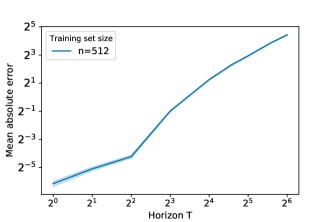
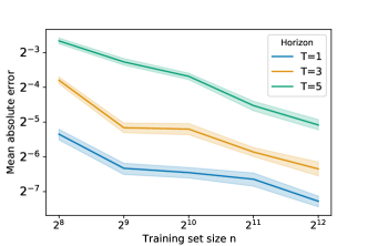
(a)                                                                      (b)

Figure 2: Simulation results for OPE errors $|\widehat{{\mathcal{V}}}(\pi)-{\mathcal{V}}(\pi)|$. Mean absolute errors (solid lines) and their standard error bands (shaded regions) are displayed for different combinations of $(n,T)$.

We choose ${\mathcal{F}}^{(t)}$ and ${\mathcal{H}}^{(t)}$ as RKHSs endowed with Gaussian kernels, with bandwidths selected according to the median heuristic trick by Fukumizu et al. (2009) for each $1\leq t\leq T$. The pool of scaling factors SCALE contains 30 positive numbers spaced evenly on a log scale between 0.001 to 0.05. The number of cross-validation partition $K=5$. The true target policy value of $\pi$ is estimated by the mean cumulative rewards of $50,000$ Monte Carlo trajectories with policy $\pi$. We compare our OPE estimator $\widehat{\mathcal{V}}(\pi)$ with the target policy value by computing mean absolute error (MAE) for each setting of $(n,T)$, as reported in Figure 2. Figure 2 validate the derived finite-sample error bound of our OPE estimator in Theorem 6.3. Specifically, Figure 2 (a) shows that the OPE estimation error is polynomial in $T$, but with an order slightly smaller than $\mathop{}\mathopen{}\mathcal{O}\mathopen{}(T^{7/2})$ as stated in Theorem 6.3. Figure 2 (b) shows that the convergence rate in terms of the sample size $n$ for our OPE estimator is slower than $\mathop{}\mathopen{}\mathcal{O}\mathopen{}(n^{-1/2})$, which also justifies our theoretical results.

8 Discussion

In this paper, we propose a non-parametric identification and estimation method for OPE in episodic confounded POMDPs with continuous states, relying on time-dependent proxy variables. We develop a fitted-$Q$-evaluation-type algorithm for estimating the $V$-bridge functions sequentially and for OPE based on the estimated $V$-bridges. The first finite-sample error bound for estimating the policy value under confounded POMDPs is established, which achieves a polynomial order with respect to the sample size and the length of horizon. Our OPE results can serve as a foundation for developing new policy optimization algorithms in the confounded POMDP, which We will leave for future work.

Supplementary Material:
Off-Policy Evaluation for Episodic Partially Observable Markov Decision Processes under Non-Parametric Models

List of Notations

${\mathcal{M}}$	the episodic and confounded POMDP
$S_{t}\in{\mathcal{S}}$	observed state at $t$ and observed state space
$U_{t}\in{\mathcal{U}}$	unobserved state at $t$ and unobserved state space
$A_{t}\in{\mathcal{A}}$	action at $t$ and discrete action space
$T$	length of horizon
$r=\{r_{t}\}_{t=1}^{T}$	reward functions over ${\mathcal{S}}\times{\mathcal{U}}\times{\mathcal{A}}$
$R_{t}$	reward at $t$
$W_{t}\in{\mathcal{W}}$	reward-proxy variable at $t$ and corresponding space
$Z_{t}\in{\mathcal{W}}$	action-proxy variable at $t$ and corresponding space
$X_{t,i}$	variable $X$ at $t$ from sample trajectory $i$
$\pi=\{\pi_{t}\}_{t=1}^{T}$	target policy depending on $S_{t}$
$\tilde{\pi}_{t}^{b}$	behavior policy at $t$ depending on $S_{t},U_{t}$
$V_{t}^{\pi}(s,u)$	state value function
${\mathcal{V}}(\pi)$ ($\widehat{{\mathcal{V}}}(\pi)$)	(estimated) policy value of a target policy $\pi$
$v^{\pi}_{t}$ ($\hat{v}^{\pi}_{t}$)	(estimated) V-bridge function (or V-bridge for short) at $t$
$q^{\pi}_{t}$ ($\hat{q}^{\pi}_{t}$)	(estimated) Q-bridge function (or Q-bridge for short) at $t$
$\widetilde{{\mathcal{P}}}_{t}$	operator $[\widetilde{{\mathcal{P}}}_{t}](Z_{t},S_{t},A_{t})={\mathbb{E}}[g(R_{t},W_{t+1},S_{t+1})\mid Z_{t},S_{t},A_{t}]$
$\overline{{\mathcal{P}}_{t}}$	operator $[\overline{{\mathcal{P}}}_{t}](Z_{t},S_{t},A_{t})={\mathbb{E}}[h(W_{t},S_{t},A_{t})\mid Z_{t},S_{t},A_{t}]$
${\mathcal{P}}_{t}$ ($\widehat{{\mathcal{P}}}_{t}$)	operator ${\mathcal{P}}_{t}g=\overline{{\mathcal{P}}_{t}}^{-1}\widetilde{{\mathcal{P}}}_{t}g$ (estimator of ${\mathcal{P}}_{t}$ defined in (7))
${\mathcal{P}}^{\pi}_{t}$ ($\widehat{{\mathcal{P}}}^{\pi}_{t}$)	operator ${\mathcal{P}}^{\pi}_{t}g=\langle\pi_{t},{\mathcal{P}}_{t}g\rangle$ (estimator of ${\mathcal{P}}^{\pi}_{t}$: $\widehat{{\mathcal{P}}}^{\pi}_{t}g=\left\langle\pi_{t},\widehat{{\mathcal{P}}}_{t}g\right\rangle$)
${\mathcal{H}}^{(t)}$	user-defined function space on ${\mathcal{W}}\times{\mathcal{S}}\times{\mathcal{A}}$
${\mathcal{F}}^{(t)}$	user-defined function space on ${\mathcal{Z}}\times{\mathcal{S}}\times{\mathcal{A}}$
${\mathcal{G}}^{(t)}$	user-defined function space on ${\mathcal{Z}}\times{\mathcal{S}}$
${\mathcal{R}}_{n}({\mathcal{F}},\delta)$	local Rademacher complexity for function class ${\mathcal{F}}$ and radius $\delta>0$
$\widehat{{\mathcal{R}}}_{n}({\mathcal{F}},\delta)$	local empirical Rademacher complexity for function class ${\mathcal{F}}$ and radius $\delta>0$
$N_{n}(\epsilon,{\mathcal{G}})$	the smallest empirical $\epsilon$-covering number of ${\mathcal{G}}$
$\alpha{\mathcal{F}}$	$\alpha{\mathcal{F}}=\{\alpha f:f\in{\mathcal{F}}\}$ for some $\alpha\in{\mathbb{R}}$
${\mathcal{F}}_{B}$	${\mathcal{F}}_{B}=\{f\in{\mathcal{F}}:\|f\|_{{\mathcal{F}}}^{2}\leq B\}$ for any $B>0$
$\|\mbox{{\rm proj}}_{t}f\|_{2}$	$\|\mbox{{\rm proj}}_{t}f\|_{2}=\sqrt{{\mathbb{E}}\{f(X)\mid Z_{t},S_{t},A_{t}\}^{2}}$
$\bar{\tau}_{1}$	ill-posedness $\bar{\tau}_{1}=\sup_{g\in{\mathcal{G}}^{(1)}}\|g(W_{1},S_{1})\|_{2}/\|{\mathbb{E}}[g(W_{1},S_{1})\mid Z_{1},S_{1}]\|_{2}$
$\tau_{t}$	ill-posedness $\tau_{t}=\sup_{h\in{\mathcal{H}}^{(t)}}\|h(W_{t},S_{t},A_{t})\|_{2}/\|\mbox{{\rm proj}}_{t}h(W_{t},S_{t},A_{t})\|_{2}$
$C_{t^{\prime},t^{\prime}-1}^{(t)}$	one-step transition ill-posedness defined after Corollary 6.2
${\mathbb{V}}({\mathcal{F}})$	VC dimension of ${\mathcal{F}}$
$\zeta(\alpha)$	Riemann Zeta function $\zeta(\alpha)=\sum_{n=1}^{\infty}(1/n)^{\alpha}$
$\text{Ker}(K)$	$\text{Ker}(K)=\{g:Kg=0\}$ null space of linear operator $K$
$A^{\perp}$	orthogonal complement of space $A$
$|{\mathcal{Z}}|$	cardinality of class $Z$

Table 1: List of Notations

Appendix A Additional Identification Assumptions

In this section, we list Assumptions 3-7 which are needed for Theorem 4.1.

A.1 Basic assumptions on the confounded POMDP structure

For the confounded POMDP with trajectory $\left(U_{t},S_{t},W_{t},Z_{t},A_{t},R_{t}\right)_{t=1}^{T}$, we list three basic assumptions below. Let $\models$ and $\cancel{\rotatebox[origin={c}]{90.0}{$\models$}}$ denote statistical independence and dependence respectively.

Assumption 3 (Markovian).

For all $1\leq t\leq T$, the time-variant transition kernel ${\mathbb{P}}_{t}$ satisfies that for any $(s,u)\in{\mathcal{S}}\times{\mathcal{U}}$, $a\in{\mathcal{A}}$ and set $F\in{\mathcal{B}}({\mathcal{S}}\times{\mathcal{U}})$,

$$\Pr((S_{t+1},U_{t+1})\in F\mid S_{t}=s,U_{t}=u,A_{t}=a,\{S_{j},U_{j},A_{j}\}_{1\leq j<t})$$

$$={\mathbb{P}}_{t}((S_{t+1},U_{t+1})\in F\mid S_{t}=s,U_{t}=u,A_{t}=a),$$

where ${\mathcal{B}}({\mathcal{S}}\times{\mathcal{U}})$ is the family of Borel subsets of ${\mathcal{S}}\times{\mathcal{U}}$ and $\{S_{j},U_{j},A_{j}\}_{1\leq j<t}\neq\emptyset$ if $t=1$.

Assumption 4 (Reward proxy).

$W_{t}\rotatebox[origin={c}]{90.0}{$\models$}(A_{t},U_{t-1},S_{t-1})\mid U_{t},S_{t}$ and $W_{t}\cancel{\rotatebox[origin={c}]{90.0}{$\models$}}U_{t}\mid S_{t}$ for $1\leq t\leq T$.

Assumption 5 (Action proxy).

$Z_{t}\rotatebox[origin={c}]{90.0}{$\models$}W_{t}\mid(U_{t},S_{t},A_{t})$, $Z_{t}\rotatebox[origin={c}]{90.0}{$\models$}R_{t}\mid(U_{t},S_{t},A_{t})$ and $Z_{t}\rotatebox[origin={c}]{90.0}{$\models$}(S_{t+1},W_{t+1})\mid(U_{t},S_{t},A_{t})$, $1\leq t\leq T$.

It can be easily verified that the DAG in Figure 1 satisfies Assumptions 3-5. Assumption 3 requires that given the current full state and action $(U_{t},S_{t},A_{t})$, the future are independent of the past.

Assumption 4 requires that the reward proxy $W_{t}$ is associated with the hidden state $U_{t}$ after adjusting observed state $S_{t}$ but $W_{t}$ is not causally affected by action $A_{t}$ and past state $(U_{t-1},S_{t-1})$ after adjusting the full current state $(U_{t},S_{t})$. This assumption does not restrict the association between $W_{t}$ and $R_{t}$. Assumption 5 requires that upon conditioning on the current full state and action tuple $(U_{t},S_{t},A_{t})$, the action proxy $Z_{t}$ does not affect the reward proxy $W_{t}$ and outcomes $R_{t},S_{t+1},W_{t+1}$ after the action $A_{t}$. Again, this assumption does not restrict the association between $Z_{t}$ and $A_{t}$.

However, based on above three assumptions, we cannot directly identify the value of target policy $\pi$ by adjusting $(U_{t},S_{t})$ since $U_{t}$ is unobserved. In addition to Assumptions 4 and 5, we also need Assumption 6 to be stated in Section A.2 below to get around the hidden state $U_{t}$.

A.2 Assumptions on the existence of bridge functions

Assumption 6 (Completeness).

For any $(s,a)\in{\mathcal{S}}\times{\mathcal{A}}$, $t=1,\dots,T$,

1. For any square-integrable function $g$, ${\mathbb{E}}\{g(U_{t})\mid Z_{t},S_{t}=s,A_{t}=a\}=0$ a.s. if and only if $g=0$ a.s;

2. For any square-integrable function $g$, ${\mathbb{E}}\{g(Z_{t})\mid W_{t},S_{t}=s,A_{t}=a\}=0$ a.s. if and only if $g=0$ a.s.

Completeness is a commonly made technical assumption in value identification problems, e.g., instrumental variable identification [Newey and Powell, 2003, D’Haultfoeuille, 2011, Chen et al., 2014], and proximal causal inference [Miao et al., 2018a, b, Tchetgen Tchetgen et al., 2020]. Together with the regularity conditions in Assumption 7, we can ensure the existence of $Q$-bridges $q^{\pi}_{t}$ and $V$-bridges $v^{\pi}_{t}$, $1\leq t\leq T$.

For a probability measure function $\mu$, let ${\mathcal{L}}^{2}\{\mu(x)\}$ denote the space of all squared integrable functions of $x$ with respect to measure $\mu(x)$, which is a Hilbert space endowed with the inner product $\left\langle g_{1},g_{2}\right\rangle=\int g_{1}(x)g_{2}(x){\rm d}\mu(x)$. For all $s,a,t$, define the following operator

$$K_{s,a;t}:{\mathcal{L}}^{2}\left\{\mu_{W_{t}\mid S_{t},A_{t}}(w\mid s,a)\right\} \rightarrow{\mathcal{L}}^{2}\left\{\mu_{Z_{t}\mid S_{t},A_{t}}(z\mid s,a)\right\}$$

$$h \mapsto{\mathbb{E}}\left\{h(W_{t})\mid Z_{t}=z,S_{t}=s,A_{t}=a\right\},$$

and its adjoint operator

$$K_{s,a;t}^{*}:{\mathcal{L}}^{2}\left\{\mu_{Z_{t}\mid S_{t},A_{t}}(z\mid s,a)\right\} \rightarrow{\mathcal{L}}^{2}\left\{\mu_{W_{t}\mid S_{t},A_{t}}(w\mid s,a)\right\}$$

$$g \mapsto{\mathbb{E}}\left\{g(Z_{t})\mid W_{t}=w,S_{t}=s,A_{t}=a\right\}.$$

Assumption 7 (Regularity Conditions).

For any $Z_{t}=z,S_{t}=s,W_{t}=w,A_{t}=a$ and $1\leq t\leq T$,

1. $\iint_{{\mathcal{W}}\times{\mathcal{Z}}}f_{W_{t}\mid Z_{t},S_{t},A_{t}}(w\mid z,s,a)f_{Z_{t}\mid W_{t},S_{t},A_{t}}(z\mid w,s,a){\rm d}w{\rm d}z<\infty$, where $f_{W_{t}\mid Z_{t},S_{t},A_{t}}$ and $f_{Z_{t}\mid W_{t},S_{t},A_{t}}$ are conditional density functions.

2. For any $g\in{\mathcal{G}}^{(t+1)}$,

   $$\int_{{\mathcal{Z}}}\left[{\mathbb{E}}\left\{R_{t}+g(W_{t+1},S_{t+1})\mid Z_{t}=z,S_{t}=s,A_{t}=a\right\}\right]^{2}f_{Z_{t}\mid S_{t},A_{t}}(z\mid s,a){\rm d}z<\infty.$$

3. There exists a singular decomposition $\left(\lambda_{s,a;t;\nu},\phi_{s,a;t;\nu},\psi_{s,a;t;\nu}\right)_{\nu=1}^{\infty}$ of $K_{s,a;t}$ such that for all $g\in{\mathcal{G}}^{(t+1)}$,

   $$\sum_{\nu=1}^{\infty}\lambda_{s,a;t;\nu}^{-2}\left|\left\langle{\mathbb{E}}\left\{R_{t}+g(W_{t+1},S_{t+1})\mid Z_{t}=z,S_{t}=s,A_{t}=a\right\},\psi_{s,a;t;\nu}\right\rangle\right|^{2}<\infty.$$

4. For all $1\leq t\leq T$, $v^{\pi}_{t}\in{\mathcal{G}}^{(t)}$ where ${\mathcal{G}}^{(t)}$ satisfies the regularity conditions (b) and (c) above.

Note that the existence of the singular decomposition of $K_{s,a,;t}$ in Assumption 7 (c) can be ensured by Assumption 7 (a), which is a sufficient condition for the compactness of $K_{s,a;t}$ by Lemma D.1.

For tabular $({\mathcal{U}},{\mathcal{W}},{\mathcal{Z}})$, Corollary A.1 provides a sufficient condition for Assumptions 6 and 7 [Shi et al., 2020].

Corollary A.1.

[Shi et al., 2020] Suppose that all ${\mathcal{U}}$, ${\mathcal{W}}$, and ${\mathcal{Z}}$ are tabular. If both $Z_{t}$ and $W_{t}$ have at least as many categories as $U_{t}$ for $1\leq t\leq T$, i.e., $|{\mathcal{Z}}|,|{\mathcal{W}}|\geq|{\mathcal{U}}|$ (where $|{\mathcal{X}}|$ is the cardinality of set ${\mathcal{X}}$), and transition probability matrices $P_{t}({\mathbf{W}}\mid{\mathbf{U}},s)\triangleq\left[P_{t}(w_{i}\mid u_{j},s)\right]_{w_{i}\in{\mathcal{W}},u_{j}\in{\mathcal{U}}}$ and $P_{t}({\mathbf{U}}\mid{\mathbf{Z}},a,s)\triangleq\left[P_{t}(u_{i}\mid z_{j},a,s)\right]_{u_{i}\in{\mathcal{U}},z_{j}\in{\mathcal{Z}}}$ are of full rank with rank $|{\mathcal{U}}|$ for all $a,s,t$, then Assumptions 6 and 7 hold.

A.3 Assumptions on the uniqueness of bridge functions

In general, we do not need to impose restrictions on the uniqueness of $V$-bridges $\{v^{\pi}_{t}\}_{t=1}^{T}$ for policy value identification. To simplify our theoretical analysis on the estimation error of $V$-bridges, we need the uniqueness of $V$-bridges $\{v^{\pi}_{t}\}_{t=1}^{T}$ and $Q$-bridges $\{q^{\pi}_{t}\}_{t=1}^{T}$, which can be ensured by the following Assumption 8.

Assumption 8.

For any square-integrable function $g$ and for any $(s,a)\in{\mathcal{S}}\times{\mathcal{A}}$, ${\mathbb{E}}\{g(W_{t})\mid Z_{t},S_{t}=s,A_{t}=a\}=0$ a.s. if and only $g=0$ a.s.

Corollary A.2.

Under Assumption 8 and all conditions in Theorem 4.1, the $V$-bridges $\left\{v^{\pi}_{t}\right\}_{t=1}^{T}$ that satisfy (3) and $Q$-bridges $\{q^{\pi}_{t}\}_{t=1}^{T}$ that satisfy (5) are both unique. Moreover, they can be non-parametrically identified by (4).

Proof.

Apparently it suffices to prove the uniqueness of $Q$-bridges $\{q^{\pi}_{t}\}_{t=1}^{T}$. If there is another set of $\{\tilde{q}_{t}^{\pi}\}_{t=1}^{T}$ that is also a solution to (4), then

$${\mathbb{E}}\left\{\tilde{q}_{t}^{\pi}(W_{t},S_{t},A_{t})-q^{\pi}_{t}(W_{t},S_{t},A_{t})\mid Z_{t},S_{t}=s,A_{t}=a\right\}=0,\quad\text{ a.s.}$$

By Assumption 8, $\tilde{q}_{t}^{\pi}(W_{t},s,a)=q^{\pi}_{t}(W_{t},s,a)$ a.s. for all $(s,a)\in{\mathcal{S}}\times{\mathcal{A}}$. ∎

For the tabular case, we have the following corollary for the uniqueness of $V$-bridges and $Q$-bridges.

Corollary A.3.

[Shi et al., 2020] Under the conditions in Corollary A.1, if $|{\mathcal{Z}}|=|{\mathcal{W}}|=|{\mathcal{U}}|$, then Assumptions 6–8 are satisfied.

Appendix B Additional Results

In this section, we derive finite-sample error bounds for $V$-bridge estimation and OPE when hypothesis spaces ${\mathcal{H}}^{(t)}$, ${\mathcal{G}}^{(t)}$ and testing space ${\mathcal{F}}^{(t)}$ are VC-subgraph classes or RKHSs with exponential eigen-decay. Then we discuss possible choices of proximal variables $W_{t}$ and $Z_{t}$.

B.1 Additional Finite-sample error bounds for $V$-bridge estimation and OPE

B.1.1 VC-subgraph class

Theorem B.1.

Under Assumptions 1 and 2, and the assumptions in Theorem 6.2 and Corollary 6.1, with probability at least $1-\zeta$, we have

$$\|v^{\pi}_{1}-\hat{v}^{\pi}_{1}\|_{2} \lesssim\texttt{ill}_{\max}\times\texttt{trans-ill}$$

$$\qquad\times T^{7/2}\left\{\sqrt{\frac{\max_{1\leq t\leq T}\left\{{\mathbb{V}}({\mathcal{F}}^{(t)}),{\mathbb{V}}({\mathcal{H}}^{(t)}),{\mathbb{V}}({\mathcal{G}}^{(t+1)})\right\}}{n}}+\sqrt{\frac{\log(T/\zeta)}{n}}\right\},\text{and}$$

$$|{\mathcal{V}}(\pi)-\hat{\mathcal{V}}(\pi)| \lesssim\texttt{ill}_{\max}\times\texttt{trans-ill}$$

$$\qquad\times T^{7/2}\left\{\sqrt{\frac{\max_{1\leq t\leq T}\left\{{\mathbb{V}}({\mathcal{F}}^{(t)}),{\mathbb{V}}({\mathcal{H}}^{(t)}),{\mathbb{V}}({\mathcal{G}}^{(t+1)})\right\}}{n}}+\sqrt{\frac{\log(T/\zeta)}{n}}\right\},$$

where $\texttt{trans-ill}=\max_{1\leq t\leq T}\exp\{a_{t}\zeta(\alpha_{t})\}$ with $\zeta(\alpha)=\sum_{t=1}^{\infty}t^{-\alpha}$, and $\texttt{ill}_{\max}=\tau_{\pi_{1}}\max_{1\leq t\leq T}\tau_{t}\|\pi_{t}/\pi_{t}^{b}\|_{\infty}^{2}$.

The proof of Theorem B.1 is given in Appendix C.5.

B.1.2 RKHS with exponential eigen-decay

Theorem B.2.

Under Assumptions 1 and 2, and the assumptions in Theorem 6.2 and Corollary 6.2 (2), with probability at least $1-\zeta$, we have

$$\|v^{\pi}_{1}-\hat{v}^{\pi}_{1}\|_{2} \lesssim\texttt{ill}_{\max}\times\texttt{trans-ill}\times T^{7/2}\left\{\sqrt{\frac{(\log n)^{1/\min\{\beta_{{\mathcal{H}}},\beta_{{\mathcal{G}}},\beta_{{\mathcal{F}}}\}}}{n}}+\sqrt{\frac{\log(T/\zeta)}{n}}\right\},\text{and}$$

$$|{\mathcal{V}}(\pi)-\hat{\mathcal{V}}(\pi)| \lesssim\texttt{ill}_{\max}\times\texttt{trans-ill}\times T^{7/2}\left\{\sqrt{\frac{(\log n)^{1/\min\{\beta_{{\mathcal{H}}},\beta_{{\mathcal{G}}},\beta_{{\mathcal{F}}}\}}}{n}}+\sqrt{\frac{\log(T/\zeta)}{n}}\right\}.$$

where $\texttt{trans-ill}=\max_{1\leq t\leq T}\exp\{a_{t}\zeta(\alpha_{t})\}$ with $\zeta(\alpha)=\sum_{t=1}^{\infty}t^{-\alpha}$, and $\texttt{ill}_{\max}=\tau_{\pi_{1}}\max_{1\leq t\leq T}\tau_{t}\|\pi_{t}/\pi_{t}^{b}\|_{\infty}^{2}$.

The proof of Theorem B.2 is given in Appendix C.5.

B.2 Different choices of proxy variables

Here we first provide several options on how to choose proxy variables $W_{t}$ and $Z_{t}$ satisfying basic assumptions 3 –5. Then we discuss their effect on the ill-posedness and one step estimation errors. Finally, we comment on some practical issues.

Choice of $W_{t}$.

In our confounded POMDP setting, typically we need a reward-inducing proxy $W_{t}$ to be separated from the current observations at time $t$ and satisfy the basic assumptions listed in Appendix A.1. In practice, $W_{t}$ can be some environmental variables that are correlated with the outcome $R_{t}$ but $A_{t}$ cannot affect $W_{t}$ (see Figure 3). It is worth mentioning that Bennett and Kallus [2021] and Shi et al. [2021] use (part of) the current observed state, i.e., $S_{t}$ in our paper, as the reward-inducing proxy. In their settings, given the current action $A_{t}$, only the hidden state $U_{t}$ can affect the next hidden state $U_{t+1}$ (Their $U_{t}$ is the full state variables in our setting). This requires that the proximal variables $Z_{t}$ and $W_{t}$ are able to capture the whole information of their hidden state $U_{t}$. In this case, Assumption 6 becomes harder to hold. In our setting, however, we allow part of their $U_{t}$ to be observable. We denote this part by $S_{t}$ in our paper. This can alleviate the burden on proximal variables $Z_{t}$ and $W_{t}$ to capture the whole information of their hidden $U_{t}$. Therefore, our completeness assumption 6 is relatively weaker. Moreover, Bennett and Kallus [2021] only consider the evaluation for deterministic target policies, while in our setting, a separate $W_{t}$ (other than $S_{t}$) allows us to evaluate random target policies.

We list some possible causal relationship among $W_{t}$, $(U_{t},S_{t})$ and $R_{t}$ in Figure 3. We require the causal relationship between $U_{t}$ and $W_{t}$. But the effect of $W_{t}$ on $R_{t}$ is optional. In practice, one can use the observed variables that have no direct effect on the action, for example, measurement of action independent disturbance which may not may not affect the current reward.

Figure 3: Causal relationship about $W_{t}$. Dashed arrows: optional causal effect. $W_{t}$ may or may not affect $R_{t}$.

(a) $Z_{t}$ is an IV for $A_{t}$.                     (b) $(U_{t},S_{t})\rightarrow Z_{t}$                    (c) $(U_{t},S_{t})\leftarrow Z_{t}$

Figure 4: Causal relationship about $Z_{t}$. Dashed arrows: optional causal effect $Z_{t}\rightarrow A_{t}$ or $Z_{t}\leftarrow A_{t}$ or no causal effect. (c) is incompatible with Figure 3 (b).

Figure 5: An example of $Z_{t}$ as the observed history.

Choice of $Z_{t}$.

Once we determine $W_{t}$, there are several proper choices of $Z_{t}$ that are compatible with $W_{t}$ (see Figure 4). One choice of $Z_{t}$ is the observed history up to step $t-1$, e.g., $Z_{t}=(Z_{t-1};S_{t-1},W_{t-1},A_{t-1},R_{t-1})$ with some pre-observed history before $(U_{1},S_{1})$ as $Z_{1}$. See Figure 5 for a valid example. In this case $Z_{t+1}$ contains information of $Z_{t}$ so that we expect that $C_{t^{\prime},t^{\prime}+1}^{(t)}$ tends to be smaller. However, this can enlarge the one-step errors $M_{{\mathcal{H}}}(T-t+1)^{2}\left(\bar{\delta}_{n}^{(t)}+c_{0}\sqrt{\frac{\log(c_{1}T/\zeta)}{n}}\right)$, where the upper bound of critical radii $\bar{\delta}_{n}^{(t)}$ becomes larger because the dimension of testing space ${\mathcal{F}}^{(t)}({\mathcal{Z}}\times{\mathcal{A}}\times{\mathcal{S}})$ is now $\mathop{}\mathopen{}\mathcal{O}\mathopen{}(t)$. Fortunately, these one-step errors only contribute to the final error bound for ${\cal V}(\pi)$ linearly.

In practice, to reduce the dimension of $Z_{t}$, one may use the most recent $k$-step observed history, or try to learn a low dimensional representation $\phi(Z_{t})$ of $Z_{t}$ and then replace ${\mathcal{F}}^{(t)}({\mathcal{Z}}\times{\mathcal{A}}\times{\mathcal{S}})$ by $\tilde{\mathcal{F}}^{(t)}(\phi({\mathcal{Z}})\times{\mathcal{A}}\times{\mathcal{S}})$ in (7). Similar ideas have been used in kernel IV regression [Singh, 2020].

Appendix C Technical Proofs

In this section, we provide the proofs of identification result in Section 3 and the finite sample bounds for $V$-bridges and OPE in Section 6.

C.1 Proof of Theorem 4.1

.

Part I.    We suppose there exists $q^{\pi}_{t}$ satisfying (4), $1\leq t\leq T$. Define $v^{\pi}_{T+1}=0$. Then

$${\mathbb{E}}\left\{R_{t}+v^{\pi}_{t+1}(W_{t+1},S_{t+1})\mid Z_{t},S_{t},A_{t}\right\}$$

$$= {\mathbb{E}}\left[{\mathbb{E}}\left\{R_{t}+v^{\pi}_{t+1}(W_{t+1},S_{t+1})\mid U_{t},Z_{t},S_{t},A_{t}\right\}\mid Z_{t},S_{t},A_{t}\right]$$

$$= {\mathbb{E}}\left[{\mathbb{E}}\left\{R_{t}+v^{\pi}_{t+1}(W_{t+1},S_{t+1})\mid U_{t},S_{t},A_{t}\right\}\mid Z_{t},S_{t},A_{t}\right]\text{ by Assumption \ref{ass:ActionProxy},}$$

and

$${\mathbb{E}}\left\{q^{\pi}_{t}(W_{t},S_{t},A_{t})\mid Z_{t},S_{t},A_{t}\right\}$$

$$= {\mathbb{E}}\left[{\mathbb{E}}\left\{q^{\pi}_{t}(W_{t},S_{t},A_{t})\mid U_{t},Z_{t},S_{t},A_{t}\right\}\mid Z_{t},S_{t},A_{t}\right]$$

$$= {\mathbb{E}}\left[{\mathbb{E}}\left\{q^{\pi}_{t}(W_{t},S_{t},A_{t})\mid U_{t},S_{t},A_{t}\right\}\mid Z_{t},S_{t},A_{t}\right]\text{ by Assumption \ref{ass:ActionProxy}.}$$

Therefore, by Assumption 6 (a), we have

$${\mathbb{E}}\left\{R_{t}+v^{\pi}_{t+1}(W_{t+1},S_{t+1})\mid U_{t},S_{t},A_{t}\right\}={\mathbb{E}}\left\{q^{\pi}_{t}(W_{t},S_{t},A_{t})\mid U_{t},S_{t},A_{t}\right\}\quad\text{ a.s.}$$ (10)

We will use this Bellman-like equation (10) to verify (3) and (5).

Next, we prove that such these $\{q^{\pi}_{t},v^{\pi}_{t}\}_{t=1}^{T}$ obtained by Algorithm 1 can be used as $Q$-bridges (5) and $V$-bridges (3).

First, at time $T$,

$${\mathbb{E}}^{\pi}\left(R_{T}\mid U_{T},S_{T}\right) =\sum_{a_{T}\in{\mathcal{A}}}{\mathbb{E}}\left(R_{T}\mid U_{T},S_{T},A_{T}=a_{T}\right)\pi_{T}(a_{T}\mid S_{T})$$

$$= \sum_{a_{T}\in{\mathcal{A}}}{\mathbb{E}}\left\{q^{\pi}_{T}(W_{T},S_{T},a_{T})\mid U_{T},S_{T},A_{T}=a_{T}\right\}\pi_{T}(a_{T}\mid S_{T})\text{ by \eqref{eq:bellman-like}}$$

$$= \sum_{a_{T}\in{\mathcal{A}}}{\mathbb{E}}\left\{q^{\pi}_{T}(W_{T},S_{T},a_{T})\mid U_{T},S_{T}\right\}\pi_{T}(a_{T}\mid S_{T})\text{ by Assumption \ref{ass:RewardProxy}}$$

$$= {\mathbb{E}}\left\{\sum_{a_{T}\in{\mathcal{A}}}\pi(a_{T}\mid S_{T})q^{\pi}_{T}(W_{T},S_{T},a_{T})\,\Big{|}\,U_{T},S_{T}\right\}$$

$$= {\mathbb{E}}\left\{v^{\pi}_{T}(W_{T},S_{T})\mid U_{T},S_{T}\right\}\text{ by definition of $v^{\pi}_{T}$}.$$

By induction, suppose that at time $t+1$, ${\mathbb{E}}^{\pi}\left[\sum_{t^{\prime}=t+1}^{T}R_{t^{\prime}}\mid S_{t+1},U_{t+1}\right]={\mathbb{E}}\left\{v^{\pi}_{t+1}(W_{t+1},S_{t+1})\mid S_{t+1},U_{t+1}\right\}$. Then at time $t$,

$${\mathbb{E}}^{\pi}\left(\sum_{t^{\prime}=t}^{T}R_{t^{\prime}}\,\Big{|}\,U_{t},S_{t}\right)$$

$$= {\mathbb{E}}^{\pi}\left\{R_{t}+{\mathbb{E}}^{\pi}\left(\sum_{t^{\prime}=t+1}^{T}R_{t^{\prime}}\,\Big{|}\,U_{t+1},S_{t+1},U_{t},S_{t}\right)\,\Big{|}\,U_{t},S_{t}\right\}$$

$$= {\mathbb{E}}^{\pi}\left\{R_{t}+{\mathbb{E}}^{\pi}\left(\sum_{t^{\prime}=t+1}^{T}R_{t^{\prime}}\,\Big{|}\,U_{t+1},S_{t+1}\right)\,\Big{|}\,U_{t},S_{t}\right\}\text{ by Assumption \ref{ass: Markovian}}$$

$$= {\mathbb{E}}^{\pi}\left\{R_{t}+{\mathbb{E}}\left(v^{\pi}_{t+1}(W_{t+1},S_{t+1})\,\Big{|}\,U_{t+1},S_{t+1}\right)\,\Big{|}\,U_{t},S_{t}\right\}$$

$$= {\mathbb{E}}^{\pi}\left\{R_{t}+{\mathbb{E}}\left(v^{\pi}_{t+1}(W_{t+1},S_{t+1})\,\Big{|}\,U_{t+1},S_{t+1},U_{t},S_{t}\right)\,\Big{|}\,U_{t},S_{t}\right\}\text{ by Assumption \ref{ass:RewardProxy}}$$

$$= {\mathbb{E}}^{\pi}\left\{R_{t}+v^{\pi}_{t+1}(W_{t+1},S_{t+1})\mid U_{t},S_{t}\right\}\text{ by the law of total expectation and Assumption \ref{ass:RewardProxy}}$$

$$= \sum_{a_{t}\in{\mathcal{A}}}{\mathbb{E}}\left\{R_{t}+v^{\pi}_{t+1}(W_{t+1},S_{t+1})\mid U_{t},S_{t},A_{t}=a_{t}\right\}\pi_{t}(a_{t}\mid S_{t})$$

$$= \sum_{a_{t}\in{\mathcal{A}}}{\mathbb{E}}\left\{q^{\pi}_{t}(W_{t},S_{t},a_{t})\mid U_{t},S_{t},A_{t}=a_{t}\right\}\pi_{t}(a_{t}\mid S_{t})\text{ by \eqref{eq:bellman-like}}$$

$$= \sum_{a_{t}\in{\mathcal{A}}}{\mathbb{E}}\left\{q^{\pi}_{t}(W_{t},S_{t},a_{t})\mid U_{t},S_{t}\right\}\pi_{t}(a_{t}\mid S_{t})\text{ by Assumption \ref{ass:RewardProxy}}$$

$$= {\mathbb{E}}\left\{\sum_{a_{t}\in{\mathcal{A}}}\pi(a_{t}\mid S_{t})q^{\pi}_{t}(W_{t},S_{t},a_{t})\,\Big{|}\,U_{t},S_{t}\right\}$$

$$= {\mathbb{E}}\left\{v^{\pi}_{t}(W_{t},S_{t})\mid U_{t},S_{t}\right\}\text{ by definition of $v^{\pi}_{t}$}.$$

Therefore (3) hold for all $1\leq t\leq T$. The validity of $Q$-bridge (5) can be similarly verified by restricting on $A_{t}=a$, for each $a\in{\mathcal{A}}$.

Part II.    Now we prove the existence of the solution to (4).

For $t=T,\dots,1$, by Assumption 7 (a), $K_{s,a;t}$ is a compact operator for each $(s,a)\in{\mathcal{S}}\times{\mathcal{A}}$ [Carrasco et al., 2007, Example 2.3], so there exists a singular value system stated in Assumption 7 (c) by Lemma D.1. Then by Assumption 6 (b), we have ${\rm Ker}(K_{s,a;t}^{*})={0}$, since for any $g\in{\rm Ker}(K_{s,a;t}^{*})$, we have, by the definition of ${\rm Ker}$, $K_{s,a;t}^{*}g={\mathbb{E}}\left[g(Z_{t})\mid W_{t},S_{t}=s,A_{t}=a\right]=0$, which implies that $g=0$ a.s. Therefore ${\rm Ker}(K_{s,a;t}^{*})={0}$ and ${\rm Ker}(K_{s,a;t}^{*})^{\perp}={\mathcal{L}}^{2}(\mu_{Z_{t}\mid S_{t},A_{t}}(z\mid s,a))$. By Assumption 7 (b), ${\mathbb{E}}\left\{R_{t}+g(W_{t+1},S_{t+1})\mid Z_{t}=\cdot,S_{t}=s,A_{t}=a\right\}\in{\rm Ker}(K_{s,a,;t}^{*})$ for given $(s,a)\in{\mathcal{S}}_{t}\times{\mathcal{A}}$ and any $g\in{\mathcal{G}}^{(t+1)}$. Now we have verified the condition (a) in Lemma D.1. The condition (b) is satisfied given Assumption 7 (c). Recursively applying the above argument from $t=T$ to $t=1$ yields the existence of the solution to (4).

∎

C.2 Proof of Theorem 6.1

By definition and Assumptions 6–8, ${\mathcal{P}}^{\pi}_{t}$, $t=1,\dots,T$, are linear operators, i.e., ${\mathcal{P}}^{\pi}_{t}(\alpha_{1}g_{1}+\alpha_{2}g_{2})=\alpha_{1}{\mathcal{P}}^{\pi}_{t}g_{1}+\alpha_{2}{\mathcal{P}}^{\pi}_{t}g_{2}$, for any $\alpha_{1},\alpha_{2}\in{\mathbb{R}}$ and $g_{1},g_{2}\in{\mathcal{L}}^{2}({\mathcal{R}}\times{\mathcal{W}}\times{\mathcal{S}})$.

We first decompose $\hat{v}^{\pi}_{t}-v^{\pi}_{t}$ into a summation of projections of one-step error. Then we bound each one-step error by the projected errors times a product of transition ill-posedness.

C.2.1 Decomposition of ${\mathcal{L}}^{2}$-error of $v^{\pi}_{1}$

Following the identification procedure in Algorithm 3, we can decompose $v^{\pi}_{1}$ by

$$v^{\pi}_{1}={\mathcal{P}}^{\pi}_{1}(R_{1}+v^{\pi}_{2})={\mathcal{P}}^{\pi}_{1}(R_{1}+{\mathcal{P}}^{\pi}_{2}(R_{2}+v^{\pi}_{3}))=\dots={\mathcal{P}}^{\pi}_{1}(R_{1}+{\mathcal{P}}^{\pi}_{2}(R_{2}+{\mathcal{P}}^{\pi}_{3}(\dots+{\mathcal{P}}^{\pi}_{T}R_{T}))).$$

Similarly, according to Section 5, we have the empirical version

$$\hat{v}^{\pi}_{1}=\widehat{{\mathcal{P}}}^{\pi}_{1}(R_{1}+\hat{v}^{\pi}_{2})=\widehat{{\mathcal{P}}}^{\pi}_{1}(R_{1}+\widehat{{\mathcal{P}}}^{\pi}_{2}(R_{2}+\hat{v}^{\pi}_{3}))=\dots=\widehat{{\mathcal{P}}}^{\pi}_{1}(R_{1}+\widehat{{\mathcal{P}}}^{\pi}_{2}(R_{2}+\widehat{{\mathcal{P}}}^{\pi}_{3}(\dots+\widehat{{\mathcal{P}}}^{\pi}_{T}R_{T}))).$$

Then for each $t=1,\dots,T$, we can decompose $\hat{v}^{\pi}_{t}-v^{\pi}_{t}$ as

$$\hat{v}^{\pi}_{t}-v^{\pi}_{t} =\widehat{{\mathcal{P}}}^{\pi}_{t}(R_{t}+\hat{v}^{\pi}_{t+1})-{\mathcal{P}}^{\pi}_{t}(R_{t}+v^{\pi}_{t+1})$$

$$=[\widehat{{\mathcal{P}}}^{\pi}_{t}(R_{t}+\hat{v}^{\pi}_{t+1})-{\mathcal{P}}^{\pi}_{t}(R_{t}+\hat{v}^{\pi}_{t+1})]+[{\mathcal{P}}^{\pi}_{t}(R_{t}+\hat{v}^{\pi}_{t+1})-{\mathcal{P}}^{\pi}_{t}(R_{t}+v^{\pi}_{t+1})]$$

$$\triangleq g_{t}+[{\mathcal{P}}^{\pi}_{t}(R_{t}+\hat{v}^{\pi}_{t+1})-{\mathcal{P}}^{\pi}_{t}(R_{t}+v^{\pi}_{t+1})]$$

$$=g_{t}+{\mathcal{P}}^{\pi}_{t}[\hat{v}^{\pi}_{t+1}-v^{\pi}_{t+1}],$$ (11)

where the last equality is due the the linearity of ${\mathcal{P}}^{\pi}_{t}$, and $v^{\pi}_{T+1}=\hat{v}^{\pi}_{T+1}\triangleq 0$. Recursively we have

$$\hat{v}^{\pi}_{1}-v^{\pi}_{1}=g_{1}+{\mathcal{P}}^{\pi}_{1}g_{2}+{\mathcal{P}}^{\pi}_{1:2}g_{3}+\dots+{\mathcal{P}}^{\pi}_{1:T-1}g_{T},$$ (12)

where ${\mathcal{P}}^{\pi}_{t^{\prime}:t}\triangleq{\mathcal{P}}^{\pi}_{t^{\prime}}\dots\mathcal{P}^{\pi}_{t}$. If $t<t^{\prime}$, ${\mathcal{P}}^{\pi}_{t^{\prime}:t}\triangleq{\mathcal{I}}$, the identity operator.

By the definition of the ill-posedness and combining the above decomposition, we can obtain the discrepancy between $\hat{v}^{\pi}_{1}$ and $v^{\pi}_{1}$:

$$\|v^{\pi}_{1}-\hat{v}^{\pi}_{1}\|_{2} \leq\bar{\tau}_{1}\|{\mathbb{E}}(v^{\pi}_{1}-\hat{v}^{\pi}_{1}\mid Z_{1},S_{1})\|_{2}$$

$$\leq\bar{\tau}_{1}\sum_{t=1}^{T}\|{\mathbb{E}}({\mathcal{P}}^{\pi}_{1:t-1}g_{t}\mid Z_{1},S_{1})\|_{2}\quad\text{by the triangular inequality},$$

where $\bar{\tau}_{{}_{1}}=\sup_{g_{1}\in{\mathcal{G}}^{(1)}}\frac{\|g_{1}\|_{2}}{\|{\mathbb{E}}[g_{1}(W_{1},S_{1})\mid Z_{1},S_{1}]\|_{2}}$. This indicates that we only need to separately bound the ${\mathcal{L}}^{2}$ norm of the projected one-step error defined as

$$\|{\mathbb{E}}[{\mathcal{P}}^{\pi}_{1:t-1}g_{t}\mid Z_{1},S_{1}]\|_{2}=\|{\mathbb{E}}[{\mathcal{P}}^{\pi}_{1:t-1}(\widehat{{\mathcal{P}}}^{\pi}_{t}-{\mathcal{P}}^{\pi}_{t})(R_{t}+\hat{v}^{\pi}_{t+1})\mid Z_{1},S_{1}]\|_{2},$$ (13)

for each $t=1,\dots,T$.

C.2.2 Error bounds for projected one-step error

To study the one-step ${\mathcal{L}}^{2}$ projected error of (13), for each $t=1,\dots,T$, motivated by (13), we sequentially define the following functions:

$$g_{t} \triangleq(\widehat{{\mathcal{P}}}^{\pi}_{t}-{\mathcal{P}}^{\pi}_{t})(\hat{v}^{\pi}_{t+1}+R_{t}),$$

$$g_{t,t-1} \triangleq{\mathcal{P}}^{\pi}_{t-1}g_{t},$$

$$g_{t,t-2} \triangleq{\mathcal{P}}^{\pi}_{t-2}g_{t,t-1}={\mathcal{P}}^{\pi}_{t-2:t-1}g_{t},$$

$$\vdots$$

$$g_{t,1} \triangleq{\mathcal{P}}^{\pi}_{1}g_{t,2}={\mathcal{P}}^{\pi}_{1:t-1}g_{t}.$$

For each $1\leq t^{\prime}<t$,

$$\quad\|{\mathbb{E}}[g_{t,t^{\prime}}(W_{t^{\prime}},S_{t^{\prime}})\mid Z_{t^{\prime}},S_{t^{\prime}}]\|_{2}=\|{\mathbb{E}}\{[{\mathcal{P}}^{\pi}_{t^{\prime}}g_{t,t^{\prime}+1}](W_{t^{\prime}},S_{t^{\prime}})\mid Z_{t^{\prime}},S_{t^{\prime}}\}\|_{2}$$

$$=\|{\mathbb{E}}^{\pi_{t^{\prime}}}[g_{t,t^{\prime}+1}(W_{t^{\prime}+1},S_{t^{\prime}+1})\mid Z_{t^{\prime}},S_{t^{\prime}}]\|_{2}$$

$$\leq C_{t^{\prime}+1,t^{\prime}}^{(t)}\|{\mathbb{E}}[g_{t,t^{\prime}+1}(W_{t^{\prime}+1},S_{t^{\prime}+1})\mid Z_{t^{\prime}+1},S_{t^{\prime}+1}]\|_{2},$$

where the local transition ill-posedness $C_{t^{\prime}+1,t^{\prime}}^{(t)}$ will be defined later in (17), and the second equality is due to

$$\quad{\mathbb{E}}\{[{\mathcal{P}}^{\pi}_{t^{\prime}}g_{t,t^{\prime}+1}](W_{t^{\prime}},S_{t^{\prime}})\mid Z_{t^{\prime}},S_{t^{\prime}}\}$$

$$={\mathbb{E}}\left\{\sum_{a\in{\mathcal{A}}}\pi_{t^{\prime}}(a\mid S_{t^{\prime}})[{\mathcal{P}}_{t^{\prime}}g_{t,t^{\prime}+1}](W_{t^{\prime}},S_{t^{\prime}},A_{t^{\prime}}=a)\mid Z_{t^{\prime}},S_{t^{\prime}}\right\}$$

$$=\sum_{a\in{\mathcal{A}}}\pi_{t^{\prime}}(a\mid S_{t^{\prime}}){\mathbb{E}}\left\{[{\mathcal{P}}_{t^{\prime}}g_{t,t^{\prime}+1}](W_{t^{\prime}},S_{t^{\prime}},A_{t^{\prime}}=a)\mid Z_{t^{\prime}},S_{t^{\prime}}\right\}$$

$$=\sum_{a\in{\mathcal{A}}}\pi_{t^{\prime}}(a\mid S_{t^{\prime}}){\mathbb{E}}\left\{[{\mathcal{P}}_{t^{\prime}}g_{t,t^{\prime}+1}](W_{t^{\prime}},S_{t^{\prime}},A_{t^{\prime}})\mid Z_{t^{\prime}},S_{t^{\prime}},A_{t^{\prime}}=a\right\}$$

$$=\sum_{a\in{\mathcal{A}}}\pi_{t^{\prime}}(a\mid S_{t^{\prime}}){\mathbb{E}}\left\{g_{t,t^{\prime}+1}(W_{t^{\prime}+1},S_{t^{\prime}+1})\mid Z_{t^{\prime}},S_{t^{\prime}},A_{t^{\prime}}=a\right\}\text{ by Q-bridge}$$

$$={\mathbb{E}}^{\pi_{t^{\prime}}}\left\{g_{t,t^{\prime}+1}(W_{t^{\prime}+1},S_{t^{\prime}+1})\mid Z_{t^{\prime}},S_{t^{\prime}}\right\}.$$

Then by induction, we can show that

$$\|{\mathbb{E}}[{\mathcal{P}}^{\pi}_{1:t-1}g_{t}\mid Z_{1},S_{1}]\|_{2}\leq C_{2,1}^{(t)}\dots C_{t,t-1}^{(t)}\|{\mathbb{E}}[g_{t}\mid Z_{t},S_{t}]\|_{2}$$

Therefore,

$$\|v^{\pi}_{1}-\hat{v}^{\pi}_{1}\|_{2} \leq\bar{\tau}_{1}\sum_{t=1}^{T}\|{\mathbb{E}}[{\mathcal{P}}^{\pi}_{1:t-1}g_{t}\mid Z_{1},S_{1}]\|_{2}$$

$$\leq\bar{\tau}_{1}\sum_{t=1}^{T}C_{2,1}^{(t)}\dots C_{t,t-1}^{(t)}\|{\mathbb{E}}[g_{t}\mid Z_{t},S_{t}]\|_{2}$$

Then for each $t=1,\dots,T$, we need to bound

$$\|{\mathbb{E}}[(\widehat{{\mathcal{P}}}^{\pi}_{t}-{\mathcal{P}}^{\pi}_{t})(R_{t}+\hat{v}^{\pi}_{t+1})\mid Z_{t},S_{t}]\|_{2} \leq\|(\widehat{{\mathcal{P}}}^{\pi}_{t}-{\mathcal{P}}^{\pi}_{t})(R_{t}+\hat{v}^{\pi}_{t+1})\|_{2}$$

$$\leq\|(\widehat{{\mathcal{P}}}_{t}-{\mathcal{P}}_{t})(R_{t}+\hat{v}^{\pi}_{t+1})\|_{2}\|\pi_{t}/\pi_{t}^{b}\|_{\infty}$$

$$\leq\tau_{t}\|\mbox{{\rm proj}}_{t}(\widehat{{\mathcal{P}}}_{t}-{\mathcal{P}}_{t})(R_{t}+\hat{v}^{\pi}_{t+1})\|_{2}\|\pi_{t}/\pi_{t}^{b}\|_{\infty},$$ (14)

where $\tau_{t}$ is the local ill-posedness constant at step $t$, defined in (15).

Finally, we have

$$\|v^{\pi}_{1}-\hat{v}^{\pi}_{1}\|_{2}\leq\bar{\tau}_{1}\sum_{t=1}^{T}\left\{\prod_{t^{\prime}=1}^{t}C_{t^{\prime},t^{\prime}-1}^{(t)}\right\}\tau_{t}\|\pi_{t}/\pi_{t}^{b}\|_{\infty}\|\mbox{{\rm proj}}_{t}(\widehat{{\mathcal{P}}}_{t}-{\mathcal{P}}_{t})(R_{t}+\hat{v}^{\pi}_{t+1})\|_{2}.$$

C.3 Proof of Theorem 6.2

For $t=T,\dots,1$, we iteratively bound $\|\mbox{{\rm proj}}_{t}(\widehat{{\mathcal{P}}}_{t}-{\mathcal{P}}_{t})(R_{t}+\hat{v}^{\pi}_{t+1})\|_{2}$ by applying Lemma D.2, which depends on the critical radius of the space that contains $\hat{v}^{\pi}_{t+1}$ from the last step $t+1$. Then we give the bound of $\|\hat{v}^{\pi}_{t}\|_{{\mathcal{G}}^{(t)}}^{2}$, which will be used to calculate critical radii in next step.

C.3.1 One-step error bound

Start from $t=T$, $\hat{v}^{\pi}_{T+1}=v^{\pi}_{T+1}\triangleq 0$. By Lemma D.3, we have with probability at least $1-3\zeta$,

$$\|\mbox{{\rm proj}}_{T}(\widehat{{\mathcal{P}}}_{T}-{\mathcal{P}}_{T})R_{T}\|_{2} \lesssim\delta_{n}^{(T)}[1+\|q^{\pi}_{T}\|_{{\mathcal{H}}^{(T)}}^{2}]$$

$$\leq\delta_{n}^{(T)}[1+M_{{\mathcal{H}}}],$$

and

$$\|\hat{q}^{\pi}_{T}\|_{{\mathcal{H}}^{(T)}}^{2}=\|\widehat{{\mathcal{P}}}_{T}R_{T}\|_{{\mathcal{H}}^{(T)}}^{2}\leq\|{\mathcal{P}}_{T}R_{T}\|_{{\mathcal{H}}^{(T)}}^{2}+C=\|q^{\pi}_{T}\|_{{\mathcal{H}}^{(T)}}^{2}+C\leq 2M_{{\mathcal{H}}},$$

by Assumption 1 (4) and we let $M_{{\mathcal{H}}}\geq C$.

Iteratively, at time $1\leq t<T$, by Lemma D.2, we have with probability at least $1-4\zeta$,

$$\|\mbox{{\rm proj}}_{t}(\widehat{{\mathcal{P}}}_{t}-{\mathcal{P}}_{t})[R_{t}+\hat{v}^{\pi}_{t+1}]\|_{2} \lesssim(T-t+1)\delta_{n}^{(t)}[1+\|{\mathcal{P}}_{t}\left(\frac{R_{t}+\hat{v}^{\pi}_{t+1}}{T-t+1}\right)\|_{{\mathcal{H}}^{(t)}}^{2}]$$

$$\leq(T-t+1)\delta_{n}^{(t)}[1+(T-t+1)M_{{\mathcal{H}}}],$$

$$\lesssim M_{{\mathcal{H}}}(T-t+1)^{2}\delta_{n}^{(t)},$$

where the second inequality is due to Assumption 1 (2), $\|{\mathcal{P}}_{t}\left(\frac{R_{t}+\hat{v}^{\pi}_{t+1}}{T-t+1}\right)\|_{{\mathcal{H}}^{(t)}}^{2}\leq\|\frac{\hat{q}^{\pi}_{t+1}}{T-t}\|_{{\mathcal{H}}^{(t+1)}}^{2}\leq(T-t+1)M_{{\mathcal{H}}}$.

Also,

$$\|\frac{\hat{q}^{\pi}_{t}}{T-t+1}\|_{{\mathcal{H}}^{(t)}}^{2}=\|\widehat{{\mathcal{P}}}_{t}\left(\frac{R_{t}+\hat{v}^{\pi}_{t+1}}{T-t+1}\right)\|_{{\mathcal{H}}^{(t)}}^{2} \leq\|{\mathcal{P}}_{t}\left(\frac{R_{t}+\hat{v}^{\pi}_{t+1}}{T-t+1}\right)\|_{{\mathcal{H}}^{(t)}}^{2}+M_{{\mathcal{H}}}$$

$$\leq(T-t+2)M_{{\mathcal{H}}},$$

where $\delta_{n}^{(t)}=\bar{\delta}_{n}^{(t)}+c_{0}\sqrt{\log(c_{1}/\zeta)/n}$, $c_{0},c_{1}>0$, $\delta_{n}^{(t)}$ upper bounds the critical radii of ${\mathcal{F}}_{3M}^{(t)}({\mathcal{Z}}_{t}\times{\mathcal{S}}_{t}\times{\mathcal{A}}_{t})$, ${\bm{\Omega}}^{(t)}$ and ${\bm{\Xi}}^{(t)}$.

Since $\|\frac{\hat{v}^{\pi}_{t}}{T-t+1}\|_{{\mathcal{G}}^{(t)}}^{2}\leq C_{{\mathcal{G}}}\|\frac{\hat{q}^{\pi}_{t}}{T-t+1}\|_{{\mathcal{H}}^{(t)}}^{2}$ by Assumption 1 (3), we have that $\|\frac{\hat{v}^{\pi}_{t}}{T-t+1}\|_{{\mathcal{G}}^{(t)}}^{2}\leq C_{{\mathcal{G}}}\|\frac{\hat{q}^{\pi}_{t}}{T-t+1}\|_{{\mathcal{H}}^{(t)}}^{2}\leq C_{{\mathcal{G}}}\|\frac{\hat{q}^{\pi}_{t+1}}{T-t}\|_{{\mathcal{H}}^{(t+1)}}^{2}\leq C_{{\mathcal{G}}}(T-t+2)M_{{\mathcal{H}}}$. Therefore $\frac{\hat{v}^{\pi}_{t}}{T-t+1}\in{\mathcal{G}}_{C_{{\mathcal{G}}}(T-t+2)M_{{\mathcal{H}}}}^{(t)}$.

C.3.2 Combined Result

Finally, we replace $\zeta$ by $\zeta/(4T)$ and redefine $\delta_{n}^{(t)}=\bar{\delta}_{n}^{(t)}+c_{0}\sqrt{\log(c_{1}T/\zeta)/n}$ for $t=1,\dots,T$, and consider the intersection of above events, we have with probability at least $1-\zeta$,

$$\|\mbox{{\rm proj}}_{t}(\widehat{{\mathcal{P}}}_{t}-{\mathcal{P}}_{t})(\hat{v}^{\pi}_{t+1}+R_{t})\|_{2}\lesssim M_{{\mathcal{H}}}(T-t+1)^{2}\delta_{n}^{(t)},$$

uniformly for all $1\leq t\leq T$.

C.4 Localized ill-posedness $\tau_{t}$ and one-step transition ill-posedness $C_{t^{\prime},t^{\prime}-1}^{(t)}$

Localized ill-posedness.

By Theorem 6.2 and (14), we have that with probability at least $1-\zeta$,

$$\|{\mathbb{E}}[(\widehat{{\mathcal{P}}}^{\pi}_{t}-{\mathcal{P}}^{\pi}_{t})(R_{t}+\hat{v}^{\pi}_{t+1})\mid Z_{t},S_{t}]\|_{2}\lesssim\tau_{t}(T-t+1)^{2}M_{{\mathcal{H}}}\delta_{n}^{(t)}\|\pi_{t}/\pi_{t}^{b}\|_{\infty},$$

uniformly for all $1\leq t\leq T$, where we define the local ill-posedness [Chen and Reiss, 2011]

$$\tau_{t}\triangleq\sup_{h\in{\mathcal{H}}^{(t)}}\frac{\|h\|_{2}}{\|\mbox{{\rm proj}}_{t}h\|_{2}}\ \text{subject to } \ \|\mbox{{\rm proj}}_{t}h\|_{2}\lesssim(T-t+1)^{2}M_{{\mathcal{H}}}\delta_{n}^{(t)},$$

$$\|h\|_{{\mathcal{H}}^{(t)}}^{2}\lesssim(T-t+1)^{3}M_{{\mathcal{H}}},$$ (15)

where the bounds for $\|\mbox{{\rm proj}}_{t}h\|_{2}$ and $\|h\|_{{\mathcal{H}}^{(t)}}^{2}$ are adapted from above results in Appendix C.3.1.

We show that under further assumption on the joint distribution of $(S_{t},A_{t},W_{t},Z_{t})$, for RKHS ${\mathcal{H}}^{(t)}$ with kernel $K_{{\mathcal{H}}^{(t)}}$, the local ill-posedness can be properly controlled. By Mercer’s theorem with some regularity conditions, for any $h\in{\mathcal{H}}^{(t)}$, we have

$$h=\sum_{j=1}^{\infty}a_{j}e_{j},$$

where {$e_{j}:{\mathcal{W}}\times{\mathcal{S}}\times{\mathcal{A}}\rightarrow{\mathbb{R}}\}$ are the eigenfunctions of kernel $K_{{\mathcal{H}}^{(t)}}$ corresponding to nonincreasing eigenvalues $\{\lambda_{j}\triangleq\lambda_{j}^{\downarrow}(K_{{\mathcal{H}}^{(t)}})\}$. Then we have $\|h\|_{2}^{2}=\sum_{j}a_{j}^{2}$ and $\|h\|_{{\mathcal{H}}}^{2}=\sum_{j}a_{j}^{2}/\lambda_{j}$.

$$\|\mbox{{\rm proj}}_{t}h\|_{2}^{2}=\sum_{i,j}a_{i}a_{j}{\mathbb{E}}\left\{{\mathbb{E}}[e_{i}(W_{t},S_{t},A_{t})\mid Z_{t},S_{t},A_{t}]{\mathbb{E}}[e_{j}(W_{t},S_{t},A_{t})\mid Z_{t},S_{t},A_{t}]\right\}.$$

For $m\in{\mathbb{N}}_{+}$, let $I=\left\{1,\dots,m\right\}$, $e_{I}=(e_{1},\dots,e_{m})$ and $a_{I}=(a_{1},\dots,a_{m})$ and define

$$\Gamma_{m}\triangleq{\mathbb{E}}\left\{{\mathbb{E}}[e_{I}(W_{t},S_{t},A_{t})\mid Z_{t},S_{t},A_{t}]{\mathbb{E}}[e_{I}(W_{t},S_{t},A_{t})\mid Z_{t},S_{t},A_{t}]^{\top}\right\}.$$

With same argument as Dikkala et al. [2020], we impose the assumption that $\lambda_{\min}(\Gamma_{m})\geq\nu_{m}$ for all $m$ almost surely, which means that the projected eigenfunctions are not strongly dependent. And we further assume that for all $i\leq m<j$,

$$\left|{\mathbb{E}}\left\{{\mathbb{E}}[e_{i}(W_{t},S_{t},A_{t})\mid Z_{t},S_{t},A_{t}]{\mathbb{E}}[e_{j}(W_{t},S_{t},A_{t})\mid Z_{t},S_{t},A_{t}]\right\}\right|\leq c\nu_{m},$$ (16)

for some constant $c>0$. This implies that the projection does not destroy the orthogonality for the first $m$ eigenfunctions and eigenfunctions with indices larger than $m$ too much. Then we can bound the local measure of ill-posedness as follow.

Lemma C.1 (Dikkala et al. [2020], Lemma 11).

Suppose that $\lambda_{\min}(\Gamma_{m})\geq\nu_{m}$ and (16) holds for all $i\leq m<j$ and some constant $c>0$. Then

$$[\tau_{t}^{*}(\delta,B)]^{2}\triangleq\max_{h\in{\mathcal{H}}_{B}^{(t)}:\|\mbox{{\rm proj}}_{t}h\|_{2}\leq\delta}\|h\|_{2}^{2}\leq\min_{m\in{\mathbb{N}}_{+}}\left\{\delta^{2}/\nu_{m}+B\left(2c\sqrt{\sum_{i=1}^{\infty}\lambda_{i}}\times\sqrt{\sum^{\infty}_{j=m+1}\lambda_{j}}+\lambda_{m+1}\right)\right\}.$$

The optimal $m_{*}$ is such that $\delta^{2}/\nu_{m}\asymp B\left(2c\sqrt{\sum_{i=1}^{\infty}\lambda_{i}}\sqrt{\sum_{j=m+1}^{\infty}\lambda_{j}}+\lambda_{m+1}\right)$.

• For a mild ill-posed case, if $\lambda_{m}\leq m^{-2\alpha_{{\mathcal{H}}}}$ for $\alpha_{{\mathcal{H}}}>1/2$ and $\nu_{m}>m^{-2b}$ for $b>0$, then $m_{*}\sim\left[\delta^{2}/B\right]^{-\frac{1}{2(\alpha_{{\mathcal{H}}}-1/2+b)}}$ and thus

$$\quad\|(\widehat{{\mathcal{P}}}_{t}-{\mathcal{P}}_{t})(\hat{v}^{\pi}_{t+1}+R_{t})\|_{2}$$

$$\lesssim\tau_{t}^{*}\left[(T-t+1)^{2}M_{{\mathcal{H}}}\delta_{n}^{(t)},(T-t+1)^{3}M_{{\mathcal{H}}}\right]$$

$$\lesssim(T-t+1)^{\frac{2(\alpha_{{\mathcal{H}}}-1/2)+3b}{(\alpha_{{\mathcal{H}}}-1/2)+2b}}[\delta_{n}^{(t)}]^{\frac{\alpha_{{\mathcal{H}}}-1/2}{\alpha_{{\mathcal{H}}}-1/2+2b}}.$$

• For a severe ill-posed case, if $\lambda_{m}\leq m^{-2\alpha_{{\mathcal{H}}}}$ for $\alpha_{{\mathcal{H}}}>1/2$ and $\nu_{m}\sim e^{-m^{b}}$ for $b>0$, then $m_{*}\sim\left[\log\left(\frac{B}{\delta^{2}}\right)\right]^{\frac{1}{b}}$, by the same argument above,

$$\quad\|(\widehat{{\mathcal{P}}}_{t}-{\mathcal{P}}_{t})(\hat{v}^{\pi}_{t+1}+R_{t})\|_{2}\lesssim\left[\log\left(\frac{1}{(T-t+1)[\delta_{n}^{(t)}]^{2}}\right)\right]^{\frac{\alpha_{{\mathcal{H}}}-1/2}{2b}}(T-t+1)^{3/2}.$$

One-step transition ill-posedness.

For each $t$, from $t^{\prime}=t-1$ to $t^{\prime}=1$, we can recursively define a sequence of local transition ill-posedness as the following:

$$C_{t^{\prime}+1,t^{\prime}}^{(t)} \triangleq\sup_{g\in{\mathcal{G}}(W_{t^{\prime}+1}\times S_{t^{\prime}+1})}\frac{\|{\mathbb{E}}^{\pi_{t^{\prime}}}[g(W_{t^{\prime}+1},S_{t^{\prime}+1})\mid Z_{t^{\prime}},S_{t^{\prime}}]\|_{2}}{\|{\mathbb{E}}[g(W_{t^{\prime}+1},S_{t^{\prime}+1})\mid Z_{t^{\prime}+1},S_{t^{\prime}+1}]\|_{2}}$$

subject to $$\|{\mathbb{E}}[g(W_{t^{\prime}+1},S_{t^{\prime}+1})\mid Z_{t^{\prime}+1},S_{t^{\prime}+1}]\|_{2}$$

$$\lesssim\tau_{t}(T-t+1)^{2}M_{{\mathcal{H}}}\delta_{n}^{(t)}\|\pi_{t^{\prime}}/\pi_{t^{\prime}}^{b}\|_{\infty}\prod_{s=t^{\prime}+1}^{t-1}C_{s+1,s}^{(t)}.$$ (17)

Then we have with probability at least $1-\zeta$,

$$\|{\mathbb{E}}[{\mathcal{P}}^{\pi}_{1:t-1}(\widehat{{\mathcal{P}}}^{\pi}_{t}-{\mathcal{P}}^{\pi}_{t})(R_{t}+\hat{v}^{\pi}_{t+1})\mid Z_{t},S_{t}]\|_{2}$$

$$\leq\left\{\prod_{t^{\prime}=1}^{t}C_{t^{\prime},t^{\prime}-1}^{(t)}\right\}\tau_{t}(T-t+1)^{2}M_{{\mathcal{H}}}\delta_{n}^{(t)}\tau_{t}\|\pi_{t}/\pi_{t}^{b}\|_{\infty},$$

uniformly for all $1\leq t\leq T$.

C.5 Proofs of Theorems 6.3, B.1 and B.2

C.5.1 Decomposition of Off-Policy Value Estimation Error

Our objective is to give an upper bound of

$$\left|{\mathbb{E}}v^{\pi}_{1}(W_{1},S_{1})-{\mathbb{E}}_{n}\hat{v}^{\pi}_{1}(W_{1},S_{1})\right| \leq\left|{\mathbb{E}}v^{\pi}_{1}-{\mathbb{E}}_{n}v^{\pi}_{1}\right|+\left|{\mathbb{E}}(v^{\pi}_{1}-\hat{v}^{\pi}_{1})\right|$$

$$\quad+\left|{\mathbb{E}}_{n}(v^{\pi}_{1}-\hat{v}^{\pi}_{1})-{\mathbb{E}}(v^{\pi}_{1}-\hat{v}^{\pi}_{1})\right|$$

$$\quad=(I)+(II)+(III),$$

For (I), by applying Hoeffding’s inequality, we have with probability at least $1-\zeta/T$,

$$(I)=|{\mathbb{E}}v^{\pi}_{1}-{\mathbb{E}}_{n}v^{\pi}_{1}|\lesssim\|v^{\pi}_{1}\|_{\infty}\sqrt{\frac{\log(c_{1}T/\zeta)}{n}}\lesssim T\sqrt{\frac{\log(c_{1}T/\zeta)}{n}}.$$

For (II), obviously $(II)=|{\mathbb{E}}(v^{\pi}_{1}-\hat{v}^{\pi}_{1})|\leq{\mathbb{E}}|v^{\pi}_{1}-\hat{v}^{\pi}_{1}|\leq\|v^{\pi}_{1}-\hat{v}^{\pi}_{1}\|_{2}$.

For (III), by applying Theorem 14.20 of Wainwright [2019], we have with probability at least $1-\zeta$,

$$(III)=\left|{\mathbb{E}}_{n}(v^{\pi}_{1}-\hat{v}^{\pi}_{1})-{\mathbb{E}}(v^{\pi}_{1}-\hat{v}^{\pi}_{1})\right|\lesssim\delta_{n}^{(0)}(\|v^{\pi}_{1}-\hat{v}^{\pi}_{1}\|_{2}+T\delta_{n}^{(0)}),$$

where $\delta_{n}^{(0)}=\bar{\delta}_{n}^{(0)}+c_{0}\sqrt{\frac{\log(c_{1}T/\zeta)}{n}}$, and $\bar{\delta}_{n}^{(0)}$ is the critical radius of ${\mathcal{G}}_{C_{{\mathcal{G}}}(T+1)M_{{\mathcal{H}}}}$.

The ${\mathcal{L}}^{2}$-error $\|v^{\pi}_{1}-\hat{v}^{\pi}\|_{2}$ in the upper bounds of (II) and (III) can be bound by combining Theorems 6.1 and 6.2.

C.5.2 Applying decomposition of OPE error

By Assumption 2, we can define $\texttt{trans-ill}=\max_{1\leq t\leq T}\exp\left\{a_{t}\zeta(\alpha_{t})\right\}$ since $\prod_{t^{\prime}=1}^{t}C_{t^{\prime},t^{\prime}-1}^{(t)}\leq\exp\left\{a_{t}\zeta(\alpha_{t})\right\}$, $1\leq t\leq T$ are bounded by Corollary 6.3. Define $\texttt{ill}_{\max}=\bar{\tau}_{1}\max_{1\leq t\leq T}\tau_{t}\|\pi_{t}/\pi_{t}^{b}\|_{\infty}$.

By applying Theorems 6.1 and 6.2, and crtical radii results in Example 1 – 3 in Appendix D.3, we have the following results:

For Theorem 6.3.

With probability at least $1-\zeta$,

$$\|v^{\pi}_{1}-\hat{v}^{\pi}_{1}\|_{2} \lesssim\texttt{ill}_{\max}\times\texttt{trans-ill}\times T^{7/2}\sqrt{\log(c_{1}T/\zeta)}n^{-\frac{1}{2+\max\{1/\alpha_{{\mathcal{H}}},1/\alpha_{{\mathcal{G}}},1/\alpha_{{\mathcal{F}}}\}}}\log(n),$$

by Corollary 6.2 (1). Then by above decomposition, with probability at least $1-\zeta$,

$$|{\mathcal{V}}(\pi)-\hat{\mathcal{V}}(\pi)| \lesssim\texttt{ill}_{\max}\times\texttt{trans-ill}\times T^{7/2}\sqrt{\log(c_{1}T/\zeta)}n^{-\frac{1}{2+\max\{1/\alpha_{{\mathcal{H}}},1/\alpha_{{\mathcal{G}}},1/\alpha_{{\mathcal{F}}}\}}}\log(n).$$

For Theorem B.1.

With probability at least $1-\zeta$, with probability at least $1-\zeta$,

$$\|v^{\pi}_{1}-\hat{v}^{\pi}_{1}\|_{2} \lesssim\texttt{ill}_{\max}\times\texttt{trans-ill}$$

$$\qquad\times T^{7/2}\left\{\sqrt{\frac{\max_{1\leq t\leq T}\left\{{\mathbb{V}}({\mathcal{F}}^{(t)}),{\mathbb{V}}({\mathcal{H}}^{(t)}),{\mathbb{V}}({\mathcal{G}}^{(t+1)})\right\}}{n}}+\sqrt{\frac{\log(T/\zeta)}{n}}\right\},$$

by Corollary 6.1. Then by above decomposition, with probability at least $1-\zeta$,

$$|{\mathcal{V}}(\pi)-\hat{\mathcal{V}}(\pi)| \lesssim\texttt{ill}_{\max}\times\texttt{trans-ill}$$

$$\qquad\times T^{7/2}\left\{\sqrt{\frac{\max_{1\leq t\leq T}\left\{{\mathbb{V}}({\mathcal{F}}^{(t)}),{\mathbb{V}}({\mathcal{H}}^{(t)}),{\mathbb{V}}({\mathcal{G}}^{(t+1)})\right\}}{n}}+\sqrt{\frac{\log(T/\zeta)}{n}}\right\}.$$

For Theorem B.2.

With probability at least $1-\zeta$,

$$\|v^{\pi}_{1}-\hat{v}^{\pi}_{1}\|_{2} \lesssim\texttt{ill}_{\max}\times\texttt{trans-ill}\times T^{7/2}\left\{\sqrt{\frac{(\log n)^{1/\min\{\beta_{{\mathcal{H}}},\beta_{{\mathcal{G}}},\beta_{{\mathcal{F}}}\}}}{n}}+\sqrt{\frac{\log(T/\zeta)}{n}}\right\},$$

by Corollary 6.2 (1). Then by above decomposition,

$$|{\mathcal{V}}(\pi)-\hat{\mathcal{V}}(\pi)| \lesssim\texttt{ill}_{\max}\times\texttt{trans-ill}\times T^{7/2}\left\{\sqrt{\frac{(\log n)^{1/\min\{\beta_{{\mathcal{H}}},\beta_{{\mathcal{G}}},\beta_{{\mathcal{F}}}\}}}{n}}+\sqrt{\frac{\log(T/\zeta)}{n}}\right\}.$$

For Corollary under mild and severe ill-posed cases.

Under assumptions in main Theorem 6.3, by directly applying Lemma C.1, we have that

$$\|v^{\pi}_{1}-\hat{v}^{\pi}_{1}\|_{2} \lesssim\bar{\tau}_{1}\max_{1\leq t\leq T}\|\pi_{t}/\pi_{t}^{b}\|_{\infty}\times\texttt{trans-ill}\times\eta(n,T,\zeta,\alpha_{{\mathcal{H}}},\alpha_{{\mathcal{F}}},\alpha_{{\mathcal{G}}},b),$$

$$|{\mathcal{V}}(\pi)-\hat{\mathcal{V}}(\pi)| \lesssim\bar{\tau}_{1}\max_{1\leq t\leq T}\|\pi_{t}/\pi_{t}^{b}\|_{\infty}\times\texttt{trans-ill}\times\eta(n,T,\zeta,\alpha_{{\mathcal{H}}},\alpha_{{\mathcal{F}}},\alpha_{{\mathcal{G}}},b),$$

where, for mild ill-posed case that $\nu_{m}\sim m^{-2b}$ for $b>0$:

$$\eta(n,T,\zeta,\alpha_{\mathcal{H}},\alpha_{\mathcal{F}},\alpha_{\mathcal{G}},b)=T^{\frac{7(\alpha_{{\mathcal{H}}}-1/2)+10b}{2(\alpha_{{\mathcal{H}}}-1/2)+4b}}\left(\sqrt{\log(c_{1}T/\zeta)}n^{-\frac{1}{2+\max\{1/\alpha_{{\mathcal{H}}},1/\alpha_{{\mathcal{G}}},1/\alpha_{{\mathcal{F}}}\}}}\log(n)\right)^{\frac{(\alpha_{{\mathcal{H}}}-1/2)}{(\alpha_{{\mathcal{H}}}-1/2)+2b}}.$$

for severe ill-posed case that $\nu_{m}\sim e^{-m^{b}}$ for $b>0$:

$$\eta(n,T,\zeta,\alpha_{{\mathcal{H}}},\alpha_{{\mathcal{F}}},\alpha_{{\mathcal{G}}},b) =\sum_{t=1}^{T}(T-t+1)^{3/2}\left\{\log\frac{n^{\frac{2}{2+\max\{1/\alpha_{{\mathcal{H}}},1/\alpha_{{\mathcal{G}}},1/\alpha_{{\mathcal{F}}}\}}}}{(\log n)^{2}(T-t+1)^{2}\log(T/\zeta)^{2}}\right\}^{-\frac{\alpha_{{\mathcal{H}}}-1/2}{2b}}.$$

Appendix D Auxiliary Lemmas

In this section, we provide some auxiliary lemmas which are needed to prove Theorem 4.1 – 6.3 and their proofs.

D.1 Lemmas For Identification

Lemma D.1 (Picard’s Theorem, Theorem 15.16 of Kress [1989]).

Given Hilbert spaces ${\mathcal{H}}_{1}$ and ${\mathcal{H}}_{2}$, a compact operator $K:{\mathcal{H}}_{1}\rightarrow{\mathcal{H}}_{2}$ and its adjoint operator $K^{*}:{\mathcal{H}}_{2}\rightarrow{\mathcal{H}}_{1}$, there exists a singular system $(\lambda_{\nu},\phi_{\nu},\psi_{\nu})_{\nu=1}^{\infty}$ of $K$, with singular values $\{\lambda_{\nu}\}$ and orthogonal sequences $\{\phi_{\nu}\}\subset{\mathcal{H}}_{1}$ and $\{\psi_{\nu}\}\subset{\mathcal{H}}_{2}$ such that $K\phi_{\nu}=\lambda_{\nu}\psi_{\nu}$ and $K^{*}\psi_{\nu}=\lambda_{\nu}\phi_{\nu}$.

Given $g\in{\mathcal{H}}_{2}$, the Fredholm integral equation of the first kind $Kh=g$ is solvable if and only if

1. $g\in{\rm Ker}(K^{*})^{\perp}$ and

2. $\sum_{\nu=1}^{\infty}\lambda_{\nu}^{-2}|\left\langle g,\psi_{\nu}\right\rangle|^{2}<\infty$,

where ${\rm Ker}(K^{*})=\left\{h:K^{*}h=0\right\}$ is the null space of $K^{*}$, and ^⟂ denotes the orthogonal complement to a set.

D.2 One-step estimation error

Consider the problem of estimating a function $h$ that satisfying the conditional moment restriction

$${\mathbb{E}}\left\{g(W)-h(X)\mid Z\right\}=0,$$ (18)

where $Z\in{\mathcal{Z}}$, $X\in{\mathcal{X}}$, $W\in{\mathcal{W}}$, $h\in{\mathcal{H}}\subset\{h\in{\mathbb{R}}^{{\mathcal{X}}}:\|h\|_{\infty}\leq 1\}$, $g\in{\mathcal{G}}\subset\{g\in{\mathbb{R}}^{{\mathcal{W}}}:\|g\|_{\infty}\leq 1\}$. Suppose that $h_{g}^{*}\in{\mathcal{H}}$ is the true $h$ that satisfies the conditional moment restriction (18).

Suppose that we observe an i.i.d. sample $\{(W_{i},X_{i},Z_{i})\}_{i=1}^{n}$ of sample size $n$ drawn from an unknown distribution. Consider the minimax estimator

$$\hat{h}_{g}=\operatorname*{arg\,min}_{h\in{\mathcal{H}}}\sup_{f\in{\mathcal{F}}}\Psi_{n}(h,f,g)-\lambda\left(\|f\|_{{\mathcal{F}}}^{2}+\frac{U}{\delta^{2}}\|f\|_{n}^{2}\right)+\lambda\mu\|h\|_{{\mathcal{H}}}^{2},$$ (19)

where $\Psi_{n}(h,f,g)=n^{-1}\sum_{i=1}^{n}\{g(W_{i})-h(X_{i})\}f(Z_{i})$ with the population version $\Psi(h,f,g)={\mathbb{E}}\{g(W)-h(X)\}f(Z)$ and $\lambda,\delta,\mu,U>0$ are tuning parameters.

Lemma D.2 (${\mathcal{L}}^{2}$-error rate for minimax estimator).

Let ${\mathcal{F}}\subset\{f\in{\mathbb{R}}^{{\mathcal{Z}}}:\|f\|_{\infty}\leq 1\}$ be a symmetric and star-convex set of test functions. Define $\delta=\delta_{n}+c_{0}\sqrt{\frac{\log(c_{1}/\zeta)}{n}}$ for some univeral constants $c_{0},c_{1}>0$ and $\delta_{n}$ the upper bound of critical radii of ${\mathcal{F}}_{3U}$,

$${\bm{\Omega}}=\left\{(x,w,z)\mapsto r(h_{g}^{*}(x)-g(w))f(z):g\in{\mathcal{G}},f\in{\mathcal{F}}_{3U},r\in[0,1]\right\},$$

and

$${\bm{\Xi}}=\left\{(x,z)\mapsto r[h-h_{g}^{*}](x)f_{\Delta}^{L^{2}B}(z);h\in{\mathcal{H}},(h-h_{g}^{*})\in{\mathcal{H}}_{B},g\in{\mathcal{G}},r\in[0,1]\right\},$$

where $f_{\Delta}^{L^{2}B}=\operatorname*{arg\,min}_{f\in{\mathcal{F}}_{L^{2}B}}\|f-\mbox{{\rm proj}}_{Z}(h-h_{g}^{*})\|_{2}$. Moreover, suppose that $\forall h\in{\mathcal{H}}$, $g\in{\mathcal{G}}$, $\|f_{\Delta}-\mbox{{\rm proj}}_{Z}(h-h_{g}^{*})\|_{2}\leq\eta_{n}\lesssim\delta_{n}$, where $f_{\Delta}\in\operatorname*{arg\,inf}_{f\in{\mathcal{F}}_{L^{2}\|h-h_{g}^{*}\|_{{\mathcal{H}}}^{2}}}\|f-\mbox{{\rm proj}}_{Z}(h-h_{g}^{*})\|_{2}$. If the tuning parameters satisfy $324C_{\lambda}\delta^{2}/U\leq\lambda\leq 324C_{\lambda}^{\prime}\delta^{2}/U$ and $\mu\geq\frac{4}{3}L^{2}+\frac{18(C_{f}+1)}{B}\frac{\delta^{2}}{\lambda}$, then with probability $1-4\zeta$,

$$\sup_{g\in{\mathcal{G}}}\|\mbox{{\rm proj}}_{Z}(\hat{h}_{g}-h_{g}^{*})\|_{2}\lesssim(1+\sup_{g\in{\mathcal{G}}}\|h_{g}^{*}\|_{{\mathcal{H}}}^{2})\delta,$$

and for all $g\in{\mathcal{G}}$ uniformly,

$$\|\hat{h}_{g}\|_{{\mathcal{H}}}^{2}\leq C+\|h_{g}^{*}\|_{{\mathcal{H}}}^{2}.$$

The proof of Lemma D.2 is given in Appendix D.4.2.

Lemma D.3 (Dikkala et al. [2020], Theorem 1).

Consider the problem of estimating a function $h$ that satisfies

$${\mathbb{E}}\left\{Y-h(X)\mid Z\right\}=0,$$

where $Z\in{\mathcal{Z}}$, $X\in{\mathcal{X}}$, $W\in{\mathcal{W}}$, $h\in{\mathcal{H}}\subset\{h\in{\mathbb{R}}^{{\mathcal{X}}}:\|h\|_{\infty}\leq 1\}$, $|Y|\leq 1$. Suppose that there exists $h^{*}\in{\mathcal{H}}$ that satisfies the conditional moment equation. Suppose that we observed an i.i.d. sample $\{(Y_{i},X_{i},Z_{i})\}_{i=1}^{n}$ of sample size $n$ drawn from an unknown distribution. Consider the minimax estimator

$$\hat{h}=\operatorname*{arg\,min}_{h\in{\mathcal{H}}}\sup_{f\in{\mathcal{F}}}\Phi_{n}(h,f)-\lambda\left(\|f\|_{{\mathcal{F}}}^{2}+\frac{U}{\delta^{2}}\|f\|_{n}^{2}\right)+\lambda\mu\|h\|_{{\mathcal{H}}}^{2},$$ (20)

where $\Phi_{n}(h,f)=n^{-1}\sum_{i=1}^{n}\{Y_{i}-h(X_{i})\}f(Z_{i})$ with the population version $\Phi(h,f)={\mathbb{E}}\{Y-h(X)\}f(Z)$ and $\lambda,\delta,\mu,U>0$ are tuning parameters.

Let ${\mathcal{F}}\subset\{f\in{\mathbb{R}}^{{\mathcal{Z}}}:\|f\|_{\infty}\leq 1\}$ be a symmetric and star-convex set of test functions. Define $\delta=\delta_{n}+c_{0}\sqrt{\frac{\log(c_{1}/\zeta)}{n}}$ for some univeral constants $c_{0},c_{1}>0$ and $\delta_{n}$ the upper bound of critical radii of ${\mathcal{F}}_{3U}$ and

$$\bar{\bm{\Xi}}=\left\{(x,z)\mapsto r[h-h^{*}](x)f_{\Delta}^{L^{2}B}(z);h\in{\mathcal{H}},(h-h^{*})\in{\mathcal{H}}_{B},r\in[0,1]\right\},$$

where $f_{\Delta}^{L^{2}B}=\operatorname*{arg\,min}_{f\in{\mathcal{F}}_{L^{2}B}}\|f-\mbox{{\rm proj}}_{Z}(h-h^{*})\|_{2}$. Moreover, suppose that $\forall h\in{\mathcal{H}}$, $\|f_{\Delta}-\mbox{{\rm proj}}_{Z}(h-h^{*})\|_{2}\leq\eta_{n}\lesssim\delta_{n}$, where $f_{\Delta}\in\operatorname*{arg\,inf}_{f\in{\mathcal{F}}_{L^{2}\|h-h^{*}\|_{{\mathcal{H}}}^{2}}}\|f-\mbox{{\rm proj}}_{Z}(h-h^{*})\|_{2}$. Suppose tuning parameters satistying $324C_{\lambda}\delta^{2}/U\leq\lambda\leq 324C_{\lambda}^{\prime}\delta^{2}/U$ and $\mu\geq\frac{4}{3}L^{2}+\frac{18(C_{f}+1)}{B}\frac{\delta^{2}}{\lambda}$. Then with probability $1-3\zeta$,

$$\|\mbox{{\rm proj}}_{Z}(\hat{h}-h^{*})\|_{2}\lesssim(1+\|h^{*}\|_{{\mathcal{H}}}^{2})\delta,$$

and

$$\|\hat{h}\|_{{\mathcal{H}}}^{2}\leq C+\|h^{*}\|_{{\mathcal{H}}}^{2}.$$

D.3 Critical radii and local Rademacher complexity

In this section we list several ways to bound the critical radii of ${\mathcal{F}}_{3U}$, ${\bm{\Omega}}$ and ${\bm{\Xi}}$ for Lemmas in Appendix D.2. We restrict ${\mathcal{G}}={\mathcal{G}}_{D}=\{g\in{\mathcal{G}}:\|g\|_{{\mathcal{G}}}^{2}\leq D\}$ for some $D>0$ in this section.

D.3.1 Local Rademacher complexity bound by entropy integral

In this subsection, we introduce an entropy integral based approach to bound the local Rademacher complexity and critical radii. Similar to local Rademacher complexity, for a star-shaped and $b$-uniformly bounded function class ${\mathcal{F}}$, the local empirical Rademacher complexity, a data-dependent quantity, is defined by

$$\widehat{R}_{n}(\delta;{\mathcal{F}})\triangleq{\mathbb{E}}\left[\sup_{f\in{\mathcal{F}},\|f\|_{n}\leq\delta}|\frac{1}{n}\epsilon_{i}f(X_{i})|\,\Big{|}\,\{X_{i}\}_{i=1}^{n}\right]$$

where $\{\epsilon_{i}\}_{i=1}^{n}$ are i.i.d. Rademacher variables. The empirical critical radius $\hat{\delta}_{n}$ is the smallest positive solution to

$$\widehat{R}_{n}(\delta)\leq\frac{\delta^{2}}{b}.$$ (21)

Wainwright [2019, Proposition 14.25] gives the relationship that with probability at least $1-\zeta$,

$$\delta_{n}\leq\mathop{}\mathopen{}\mathcal{O}\mathopen{}(\hat{\delta}_{n}+\sqrt{\frac{\log(1/\zeta)}{n}}).$$

Therefore, we can study the critical radius $\delta_{n}$ by empirical critical radius $\hat{\delta}_{n}$.

Given a space ${\mathcal{G}}$, an empirical $\epsilon$-covering of ${\mathcal{G}}$ is defined as any function class ${\mathcal{G}}^{\epsilon}$ such that for all $g\in{\mathcal{G}}$, $\inf_{g_{\epsilon}\in{\mathcal{G}}^{\epsilon}}\|g_{\epsilon}-g\|_{n}\leq\epsilon$. Denote the smallest empirical $\epsilon$-covering of ${\mathcal{G}}$ by $N_{n}(\epsilon,{\mathcal{G}})$. Let ${\mathbb{B}}_{n}(\delta;{\mathcal{G}})\triangleq\left\{g\in{\mathcal{G}}:\|g\|_{n}\leq\delta\right\}$. Then we have the following Lemma to bound the empirical critical radius by Dudley’s entropy integral.

Lemma D.4.

[Wainwright, 2019, Corollary 14.3] The empirical critical inequality (21) is satisfied for any $\delta>0$ such that

$$\frac{64}{\sqrt{n}}\int_{\frac{\delta^{2}}{2b}}^{\delta}\sqrt{\log N_{n}(t,{\mathbb{B}}_{n}(\delta,{\mathcal{G}}))}{\mathrm{d}}t\leq\frac{\delta^{2}}{b}.$$

Lemma D.5.

Suppose that $\|h_{g}^{*}\|_{{\mathcal{H}}}^{2}\leq A\|g\|_{{\mathcal{G}}}^{2}$ for all $g\in{\mathcal{G}}$, so that $\|h_{g}^{*}\|_{{\mathcal{H}}}^{2}\leq AD$. Let $\widehat{\delta}_{n}>0$ satisfy the inequality

$$\frac{64}{\sqrt{n}}\int_{\frac{\delta^{2}}{2}}^{4\delta}\sqrt{\log N_{n}(t,\mbox{{\rm star}}\{{\mathcal{F}}_{3U\vee L^{2}B}\})+\log N_{n}(t,\mbox{{\rm star}}\{{\mathcal{H}}_{AD\vee B}\})+\log N_{n}(t,\mbox{{\rm star}}\{{\mathcal{G}}_{D}\})}{\rm d}t\leq\delta^{2}.$$

Then with probability $1-\zeta$, we have $\delta_{n}\leq\mathop{}\mathopen{}\mathcal{O}\mathopen{}(\widehat{\delta}_{n}+\sqrt{\frac{\log(1/\zeta)}{n}})$, where $\delta_{n}$ is the maximum critical radii of ${\mathcal{F}}_{3U}$, ${\bm{\Omega}}$ and ${\bm{\Xi}}$, with

$${\bm{\Omega}}=\left\{(x,w,z)\mapsto r(h_{g}^{*}(x)-g(w))f(z):g\in{\mathcal{G}}_{D},f\in{\mathcal{F}}_{3U},r\in[0,1]\right\}.$$

The proof of Lemma D.5 is given in Appendix D.4.3.

Example 1 (Critical radii for VC subspaces).

If star shaped ${\mathcal{F}},{\mathcal{H}}$ and ${\mathcal{G}}$ are VC subspaces with VC dimensions ${\mathbb{V}}({\mathcal{F}})$, ${\mathbb{V}}({\mathcal{H}})$ and ${\mathbb{V}}({\mathcal{G}})$, respectively, then $\log N_{n}(t,{\mathcal{F}})+\log N_{n}(t,{\mathcal{H}})+\log N_{n}(t,{\mathcal{G}})\lesssim[{\mathbb{V}}({\mathcal{F}})+{\mathbb{V}}({\mathcal{H}})+{\mathbb{V}}({\mathcal{G}})]\log(1/t)\lesssim\max\{{\mathbb{V}}({\mathcal{F}}),{\mathbb{V}}({\mathcal{H}}),{\mathbb{V}}({\mathcal{G}})\}\log(1/t)$. By Lemma D.4 and Lemma D.5, we have with probability at least $1-\zeta$, $\delta_{n}\lesssim\sqrt{\frac{\max\{{\mathbb{V}}({\mathcal{F}}),{\mathbb{V}}({\mathcal{H}}),{\mathbb{V}}({\mathcal{G}})\}}{n}}+\sqrt{\frac{\log(1/\zeta)}{n}}$, where the $\delta_{n}$ is defined in Lemma D.5.

D.3.2 Local Rademacher complexity bound for RKHSs

Lemma D.6 (Critical radii for RKHSs, Corollary 14.5 of Wainwright [2019]).

Let ${\mathcal{F}}_{B}=\left\{f\in{\mathcal{F}}\mid\|f\|_{{\mathcal{F}}}^{2}\leq B\right\}$ be the $B$-ball of a RKHS ${\mathcal{F}}$. Suppose that $K_{{\mathcal{F}}}$ is the reproducing kernel of ${\mathcal{F}}$ with eigenvalues $\{\lambda_{j}^{\downarrow}(K_{{\mathcal{F}}})\}_{j=1}^{\infty}$ sorted in a decreasing order. Then the localized population Rademacher complexity is upper bounded by

$${\mathcal{R}}_{n}({\mathcal{F}}_{B},\delta)\leq\sqrt{\frac{2B}{n}}\sqrt{\sum_{j=1}^{\infty}\min\left\{\lambda_{j}^{\downarrow}(K_{{\mathcal{F}}}),\delta^{2}\right\}}.$$

Lemma D.7 (Critical radii for ${\bm{\Omega}}$ and ${\bm{\Xi}}$ when ${\mathcal{H}}$, ${\mathcal{F}}$, ${\mathcal{G}}$ are RKHSs).

Suppose that ${\mathcal{F}}$,${\mathcal{H}}$, and ${\mathcal{G}}$ are RKHSs endowed with reproducing kernels $K_{{\mathcal{F}}}$, $K_{{\mathcal{H}}}$, and $K_{{\mathcal{G}}}$ with decreasingly sorted eigenvalues $\left\{\lambda_{j}^{\downarrow}(K_{{\mathcal{F}}})\right\}_{j=1}^{\infty}$, $\left\{\lambda_{j}^{\downarrow}(K_{{\mathcal{H}}})\right\}_{j=1}^{\infty}$, and $\left\{\lambda_{j}^{\downarrow}(K_{{\mathcal{G}}})\right\}_{j=1}^{\infty}$, respectively. Then

$${\mathcal{R}}_{n}({\bm{\Xi}},\delta)\leq LB\sqrt{\frac{2}{n}}\sqrt{\sum_{i,j=1}^{\infty}\min\left\{\lambda_{i}^{\downarrow}(K_{{\mathcal{H}}})\lambda_{j}^{\downarrow}(K_{{\mathcal{F}}}),\delta^{2}\right\}},\quad\text{and}$$

$${\mathcal{R}}_{n}({\bm{\Omega}},\delta)\leq\sqrt{D}(1+\sqrt{A})\sqrt{\frac{12U}{n}}\sqrt{\sum_{i,j=1}^{\infty}\min\left\{[(\lambda_{i}^{\downarrow}(K_{{\mathcal{H}}})+\lambda_{i}^{\downarrow}(K_{{\mathcal{G}}})]\lambda_{j}^{\downarrow}(K_{{\mathcal{F}}}),\delta^{2}\right\}}.$$

The proof of Lemma D.7 is given in Appendix D.4.4.

We give the following two examples as directly applications of Lemma D.6 and D.7.

Example 2 (Critical radii for RKHSs endowed with kernels with polynomial decay).

With the same conditions in Lemma D.7, when $\lambda_{j}^{\downarrow}(K_{{\mathcal{F}}})\leq cj^{-2\alpha_{{\mathcal{F}}}}$, $\lambda_{j}^{\downarrow}(K_{{\mathcal{G}}})\leq cj^{-2\alpha_{{\mathcal{G}}}}$, $\lambda_{j}^{\downarrow}(K_{{\mathcal{H}}})\leq cj^{-2\alpha_{{\mathcal{H}}}}$, where constant $\alpha_{{\mathcal{H}}},\alpha_{{\mathcal{G}}},\alpha_{{\mathcal{F}}}>1/2,c>0$, then by Krieg [2018] we have the upper bound of critical radii of ${\mathcal{F}}_{3U}$, ${\bm{\Omega}}$ and ${\bm{\Xi}}$ satisfies

$$\delta_{n}\lesssim\max\{\sqrt{B},LB,\sqrt{6DU}(1+\sqrt{A})\}n^{-\frac{1}{2+\max\{1/\alpha_{{\mathcal{F}}},1/\alpha_{{\mathcal{G}}},1/\alpha_{{\mathcal{H}}}\}}}\log(n).$$

Example 3 (Critical radii for RKHSs endowed with kernels with exponential decay).

With the same conditions in Lemma D.7, when $\lambda_{j}^{\downarrow}(K_{{\mathcal{H}}})\leq a_{1}e^{-a_{2}j^{\beta_{{\mathcal{H}}}}}$, $\lambda_{j}^{\downarrow}(K_{{\mathcal{G}}})\leq a_{1}e^{-a_{2}j^{\beta_{{\mathcal{G}}}}}$ and $\lambda_{j}^{\downarrow}(K_{{\mathcal{F}}})\leq a_{1}e^{-a_{2}j^{\beta_{{\mathcal{F}}}}}$, for constants $a_{1},a_{2},\beta_{{\mathcal{H}}},\beta_{{\mathcal{G}}},\beta_{{\mathcal{F}}}>0$, then we have the upper bound of critical radii of ${\mathcal{F}}_{3U}$, ${\bm{\Omega}}$ and ${\bm{\Xi}}$ satisfies

$$\delta_{n}\lesssim\max\{\sqrt{B},LB,\sqrt{6DU}(1+\sqrt{A})\}\sqrt{\frac{(\log n)^{1/\min\{\beta_{{\mathcal{F}}},\beta_{{\mathcal{G}}},\beta_{{\mathcal{H}}}\}}}{n}}.$$

D.4 Proof of Lemmas

D.4.1 Proof of Lemma C.1

Proof.

For any $m\in{\mathbb{N}}_{+}$,

$$\|\mbox{{\rm proj}}_{t}h\|_{2}^{2} =a_{I}^{\top}\Gamma_{m}a_{I}+2\sum_{i\leq m<j}a_{i}a_{j}{\mathbb{E}}\left\{{\mathbb{E}}[e_{i}(W_{t},S_{t},A_{t})\mid Z_{t},S_{t},A_{t}]{\mathbb{E}}[e_{j}(W_{t},S_{t},A_{t})\mid Z_{t},S_{t},A_{t}]\right\}$$

$$\quad+{\mathbb{E}}\left(\sum_{j>m}a_{j}{\mathbb{E}}[e_{j}(W_{t},S_{t},A_{t})\mid Z_{t},S_{t},A_{t}]\right)$$

$$\geq a_{I}^{\top}\Gamma_{m}a_{I}-2\sum_{i\leq m<j}|a_{i}a_{j}|{\mathbb{E}}\left\{{\mathbb{E}}[e_{i}(W_{t},S_{t},A_{t})\mid Z_{t},S_{t},A_{t}]{\mathbb{E}}[e_{j}(W_{t},S_{t},A_{t})\mid Z_{t},S_{t},A_{t}]\right\}$$

$$\geq a_{I}^{\top}\Gamma_{m}a_{I}-2\sum_{i\leq m<j}|a_{i}a_{j}|c\nu_{m}$$

$$\geq\nu_{m}\|a_{I}\|_{2}^{2}-2c\nu_{m}\sum_{i\leq m}|a_{i}|\sum_{j>m}|a_{j}|$$

$$\geq\nu_{m}\|a_{I}\|_{2}^{2}-2c\nu_{m}\sqrt{\sum_{i\leq m}\lambda_{i}}\sqrt{\sum_{i\leq m}\frac{|a_{i}|^{2}}{\lambda_{i}}}\sqrt{\sum_{j>m}\lambda_{j}}\sqrt{\sum_{j>m}\frac{|a_{j}|^{2}}{\lambda_{j}}}$$

$$\geq\nu_{m}\|a_{I}\|_{2}^{2}-2c\nu_{m}B\sqrt{\sum_{i=1}^{\infty}\lambda_{i}}\sqrt{\sum_{j>m}\lambda_{j}},\text{ ~{}~{}~{} since }\sum_{j=1}^{\infty}\frac{|a_{j}|^{2}}{\lambda_{j}}\leq B.$$

Therefore, $\|h\|_{2}^{2}\leq\|a_{I}\|^{2}+B\lambda_{m+1}\leq\|\mbox{{\rm proj}}_{t}h\|_{2}^{2}/\nu_{m}+2cB\sqrt{\sum_{i=1}^{\infty}\lambda_{i}}\sqrt{\sum_{j>m}\lambda_{j}}+B\lambda_{m+1}$. Because $\|\mbox{{\rm proj}}_{t}h\|_{2}\leq\delta$, by taking minimum over $m\in{\mathbb{N}}_{+}$, we have that

$$[\tau^{*}(\delta,B)]^{2}\leq\min_{m\in{\mathbb{N}}_{+}}\left\{\delta^{2}/\nu_{m}+B\left(2c\sqrt{\sum_{i=1}^{\infty}\lambda_{i}}\sqrt{\sum_{j>m}\lambda_{j}}+\lambda_{m+1}\right)\right\}.$$

∎

D.4.2 Proof of Lemma D.2

Proof.

Let ${\mathcal{H}}_{B}=\left\{h\in{\mathcal{H}}:\|h\|_{{\mathcal{H}}}^{2}\leq B\right\}$ and ${\mathcal{F}}_{U}=\left\{f\in{\mathcal{F}}:\|f\|_{{\mathcal{F}}}^{2}\leq U\right\}$. Moreover, let

$$\Psi^{\lambda}(f,g,h) =\Psi(h,f,g)-\lambda\left(\frac{2}{3}\|f\|_{{\mathcal{F}}}^{2}+\frac{U}{2\delta^{2}}\|f\|_{2}^{2}\right),\quad\text{and}$$

$$\Psi_{n}^{\lambda}(f,g,h) =\Psi_{n}(h,f,g)-\lambda\left(\|f\|_{{\mathcal{F}}}^{2}+\frac{U}{\delta^{2}}\|f\|_{n}^{2}\right).$$

We first study the relationship between the empirical penalty $\lambda\left(\|f\|_{{\mathcal{F}}}^{2}+\frac{U}{\delta^{2}}\|f\|_{n}^{2}\right)$ and population penalty $\lambda\left(\frac{2}{3}\|f\|_{{\mathcal{F}}}^{2}+\frac{U}{2\delta^{2}}\|f\|_{2}^{2}\right)$. Let $\delta=\delta_{n}+c_{0}\sqrt{\frac{\log(c_{1}/\zeta)}{n}}$, where $\delta_{n}$ upper bounds the critical radius of ${\mathcal{F}}_{3U}$ and $c_{0},c_{1}$ are universal constants, by Theorem 14.1 of Wainwright [2019], with probablity $1-\zeta$, uniformly for any $f\in{\mathcal{F}}$, we have

$$\left|\|f\|_{n}^{2}-\|f\|_{2}^{2}\right|\leq\frac{1}{2}\|f\|_{2}^{2}+\delta^{2}\max\left\{1,\frac{\|f\|_{{\mathcal{F}}}^{2}}{3U}\right\},\text{and thus}$$ (22)

$$\|f\|_{{\mathcal{F}}}^{2}+\frac{U}{\delta^{2}}\|f\|_{n}^{2} \geq\|f\|_{{\mathcal{F}}}^{2}+\frac{U}{\delta^{2}}\left[\frac{1}{2}\|f\|_{2}^{2}-\delta^{2}\max\left\{1,\frac{\|f\|_{{\mathcal{F}}}^{2}}{3U}\right\}\right]$$

$$\geq\|f\|_{{\mathcal{F}}}^{2}+\frac{U}{2\delta^{2}}\|f\|_{2}^{2}-\max\left\{U,\frac{1}{3}\|f\|_{{\mathcal{F}}}^{2}\right\}$$

$$\geq\frac{2}{3}\|f\|_{{\mathcal{F}}}^{2}+\frac{U}{2\delta^{2}}\|f\|_{2}^{2}-U.$$ (23)

In the following proof, we obtain the error rate of the uniform projected RMSE $\sup_{g\in{\mathcal{G}}}\|\mbox{{\rm proj}}_{Z}(\hat{h}_{g}-h_{g}^{*})\|_{2}$ by combinding upper and lower bounds of the sup-loss

$$\sup_{f\in{\mathcal{F}}}\Psi_{n}(\hat{h}_{g},f,g)-\Psi_{n}(h_{g}^{*},f,g)-2\lambda\left(\|f\|_{{\mathcal{F}}}^{2}+\frac{U}{\delta^{2}}\|f\|_{n}^{2}\right).$$ (24)

Upper bound of sup-loss (24).

By a simple decomposition of $\Psi_{n}^{\lambda}(h,f,g)$, we have

$$\Psi_{n}^{\lambda}(h,f,g) =\Psi_{n}(h,f,g)-\Psi_{n}(h_{g}^{*},f,g)+\Psi_{n}(h_{g}^{*},f,g)-\lambda\left(\|f\|_{{\mathcal{F}}}^{2}+\frac{U}{\delta^{2}}\|f\|_{n}^{2}\right)$$

$$\geq\Psi_{n}(h,f,g)-\Psi_{n}(h_{g}^{*},f,g)-2\lambda\left(\|f\|_{{\mathcal{F}}}^{2}+\frac{U}{\delta^{2}}\|f\|_{n}^{2}\right)$$

$$\quad+\inf_{f\in{\mathcal{F}}}\left\{\Psi_{n}(h_{g}^{*},f,g)+\lambda\left(\|f\|_{{\mathcal{F}}}^{2}+\frac{U}{\delta^{2}}\|f\|_{n}^{2}\right)\right\}$$

$$=\Psi_{n}(h,f,g)-\Psi_{n}(h_{g}^{*},f,g)-2\lambda\left(\|f\|_{{\mathcal{F}}}^{2}+\frac{U}{\delta^{2}}\|f\|_{n}^{2}\right)$$

$$\quad-\sup_{f\in{\mathcal{F}}}\Psi_{n}^{\lambda}(h_{g}^{*},f,g),\quad\text{since ${\mathcal{F}}$ is symmetric about $0$.}$$

Taking $\sup_{f\in{\mathcal{F}}}$ on both sides and picking $h\leftarrow\hat{h}_{g}$ yields the basic inequality:

$$\sup_{f\in{\mathcal{F}}}\Psi_{n}(\hat{h}_{g},f,g)-\Psi_{n}(h_{g}^{*},f,g)-2\lambda\left(\|f\|_{{\mathcal{F}}}^{2}+\frac{U}{\delta^{2}}\|f\|_{n}^{2}\right)$$

$$\leq \sup_{f\in{\mathcal{F}}}\Psi_{n}^{\lambda}(h_{g}^{*},f,g)+\sup_{f\in{\mathcal{F}}}\Psi_{n}^{\lambda}(\hat{h}_{g},f,g)$$

$$\leq 2\sup_{f\in{\mathcal{F}}}\Psi_{n}^{\lambda}(h_{g}^{*},f,g)+\lambda\mu(\|h_{g}^{*}\|_{{\mathcal{H}}}^{2}-\|\hat{h}_{g}\|_{{\mathcal{H}}}^{2}),$$ (25)

where the last inequality is given by the definition of $\hat{h}_{g}$ in (19). Now it suffices to obtain the upper bound of $\sup_{f\in{\mathcal{F}}}\Psi_{n}^{\lambda}(h_{g}^{*},f,g)$ uniformly over $g\in{\mathcal{G}}$.

For upper bound of $\sup_{f\in{\mathcal{F}}}\Psi_{n}^{\lambda}(h_{g}^{*},f,g)$.

By the assumption that $\|g\|_{\infty}\leq 1$, $\|h\|_{\infty}\leq 1$ and $\|f\|_{\infty}\leq 1$, we have $\|\frac{1}{2}\left\{g(W)-h(X)\right\}f(Z)\|_{\infty}\leq 1$. Then we apply Lemma 11 of Foster and Syrgkanis [2019], with ${\mathcal{L}}_{\frac{1}{2}(g-h_{g}^{*})f}=\frac{1}{2}(g-h_{g}^{*})f$. Let $\delta_{n}$ be the upper bound of critical radii of ${\bm{\Omega}}$. By choosing $\delta=\delta_{n}+c_{0}\sqrt{\frac{\log(c_{1}/\zeta)}{n}}$, we have with probability $1-\zeta$, uniformly for any $f\in{\mathcal{F}}_{3U}$ and $g\in{\mathcal{G}}$:

$$\frac{1}{2}\left|\left\{\Psi_{n}(h_{g}^{*},f,g)-\Psi_{n}(h_{g}^{*},0,g)\right\}-\left\{\Psi(h_{g}^{*},f,g)-\Psi(h_{g}^{*},0,g)\right\}\right|$$

$$\leq 18\delta\left(\|\frac{1}{2}(g-h_{g}^{*})f\|_{2}+\delta\right)$$

$$\leq 18\delta\left(\|f\|_{2}+\delta\right),$$

where, by definition, $\Psi_{n}(h_{g}^{*},0,g)=\Psi(h_{g}^{*},0,g)=0$. If $\|f\|_{{\mathcal{F}}}^{2}\geq 3U$, applying the above inequality with $f\leftarrow f\sqrt{3U}/\|f\|_{{\mathcal{F}}}$, we have with probability $1-\zeta$, for all $f\in{\mathcal{F}}$ and $g\in{\mathcal{G}}$:

$$\left|\Psi_{n}(h_{g}^{*},f,g)-\Psi(h_{g}^{*},f,g)\right| \leq 36\delta\left\{\|f\|_{2}+\max\left\{1,\frac{\|f\|_{{\mathcal{F}}}}{\sqrt{3U}}\right\}\delta\right\}$$

$$\leq 36\delta\left\{\|f\|_{2}+\left(1+\frac{\|f\|_{{\mathcal{F}}}}{\sqrt{3U}}\right)\delta\right\}.$$ (26)

By using (26) and (23) sequentially, we have with probability $1-2\zeta$, for all $f\in{\mathcal{F}}$ and $g\in{\mathcal{G}}$:

$$\Psi_{n}^{\lambda}(h_{g}^{*},f,g)=\Psi_{n}(h_{g}^{*},f,g)-\lambda\left(\|f\|_{{\mathcal{F}}}^{2}+\frac{U}{\delta^{2}}\|f\|_{n}^{2}\right)$$

$$\leq \Psi(h_{g}^{*},f,g)+36\delta\left\{\|f\|_{2}+\left(1+\frac{\|f\|_{{\mathcal{F}}}}{\sqrt{3U}}\right)\delta\right\}-\lambda\left(\|f\|_{{\mathcal{F}}}^{2}+\frac{U}{\delta^{2}}\|f\|_{n}^{2}\right)$$

$$\leq \Psi(h_{g}^{*},f,g)+36\delta\left\{\|f\|_{2}+\left(1+\frac{\|f\|_{{\mathcal{F}}}}{\sqrt{3U}}\right)\delta\right\}-\lambda\left(\frac{2}{3}\|f\|_{{\mathcal{F}}}^{2}+\frac{U}{2\delta^{2}}\|f\|_{2}^{2}\right)+\lambda U$$

$$= \Psi^{\lambda/2}(h_{g}^{*},f,g)+36\delta^{2}+\lambda U+\left(36\delta\|f\|_{2}-\frac{\lambda U}{4\delta^{2}}\|f\|_{2}^{2}\right)+\left(\frac{36\delta}{\sqrt{3U}}\delta\|f\|_{{\mathcal{F}}}-\frac{\lambda}{3}\|f\|_{{\mathcal{F}}}^{2}\right).$$

With the assumption that $\lambda\geq 324C_{\lambda}\delta^{2}/U$, by completing squares, we have

$$36\delta\|f\|_{2}-\frac{\lambda U}{4\delta^{2}}\|f\|_{2}^{2}\leq\frac{(36\delta)^{2}}{4\frac{\lambda U}{4\delta^{2}}}\leq\frac{4\delta^{2}}{C_{\lambda}},\quad\text{ and}$$

$$\frac{36\delta^{2}}{\sqrt{3U}}\|f\|_{{\mathcal{F}}}-\frac{\lambda}{3}\|f\|_{{\mathcal{F}}}^{2}\leq\frac{324\delta^{4}}{\lambda U}\leq\frac{\delta^{2}}{C_{\lambda}}.$$

Therefore, with probability $1-2\zeta$, for all $f\in{\mathcal{F}}$ and $g\in{\mathcal{G}}$:

$$\Psi_{n}^{\lambda}(h_{g}^{*},f,g)\leq\Psi^{\lambda/2}(h_{g}^{*},f,g)+\lambda U+\left(36+\frac{5}{C_{\lambda}}\right)\delta^{2}.$$ (27)

Now we go back to (25). By applying two upper bounds above, we have with probability $1-2\zeta$, uniformly for all $g\in{\mathcal{G}}$:

$$\sup_{f\in{\mathcal{F}}}\Psi_{n}(\hat{h}_{g},f,g)-\Psi_{n}(h_{g}^{*},f,g)-2\lambda\left(\|f\|_{{\mathcal{F}}}^{2}+\frac{U}{\delta^{2}}\|f\|_{n}^{2}\right)$$

$$\leq 2\sup_{f\in{\mathcal{F}}}\Psi_{n}^{\lambda}(h_{g}^{*},f,g)+\lambda\mu(\|h_{g}^{*}\|_{{\mathcal{H}}}^{2}-\|\hat{h}_{g}\|_{{\mathcal{H}}}^{2})$$

$$\leq 2\sup_{f\in{\mathcal{F}}}\Psi^{\lambda/2}(h_{g}^{*},f,g)+2\lambda U+(72+10/C_{\lambda})\delta^{2}+\lambda\mu(\|h_{g}^{*}\|_{{\mathcal{H}}}^{2}-\|\hat{h}_{g}\|_{{\mathcal{H}}}^{2})$$

$$= 2\lambda U+(72+10/C_{\lambda})\delta^{2}+\lambda\mu(\|h_{g}^{*}\|_{{\mathcal{H}}}^{2}-\|\hat{h}_{g}\|_{{\mathcal{H}}}^{2}),$$ (28)

where $\sup_{f\in{\mathcal{F}}}\Psi^{\lambda/2}(h_{g}^{*},f,g^{*})=0$ since ${\mathbb{E}}\left\{g(W)-h_{g}^{*}(X)\right\}f(Z)=0$.

We can also obtain the upper bound of $\|\hat{h}_{g}\|_{{\mathcal{H}}}$ by (28). By choosing $f=0$, the LHS of (28) is 0, so the supremum of LHS is nonnegative. Then with probability $1-2\zeta$,

$$\|\hat{h}_{g}\|_{{\mathcal{H}}}^{2} \leq\frac{1}{\lambda\mu}\Big{\{}2\lambda U+(72+10/C_{\lambda})\delta^{2}\Big{\}}+\|h_{g}^{*}\|_{{\mathcal{H}}}^{2}$$

$$\leq\frac{36C_{\lambda}+3+\frac{5}{9C_{\lambda}}}{\frac{24C_{\lambda}L^{2}}{U}+\frac{C_{f}+1}{B}}+\|h_{g}^{*}\|_{{\mathcal{H}}}^{2}.$$ (29)

Lower bound of sup-loss (24).

For any $h$ and $g$, by our assumption that $\|f_{\Delta}-\mbox{{\rm proj}}_{Z}(h-h_{g}^{*})\|_{2}\leq\eta_{n}$, where $f_{\Delta}=\operatorname*{arg\,min}_{f\in{\mathcal{F}}_{L^{2}\|h-h_{g}^{*}\|_{{\mathcal{H}}}^{2}}}\|f-\mbox{{\rm proj}}_{Z}(h-h_{g}^{*})\|_{2}$. Let $\widehat{\Delta}_{g}=\hat{h}_{g}-h_{g}^{*}$, and $f_{\widehat{\Delta}_{g}}=\operatorname*{arg\,min}_{f\in{\mathcal{F}}_{L^{2}\|\hat{h}_{g}-h^{*}_{g}\|_{{\mathcal{H}}}}}\|f-\mbox{{\rm proj}}_{Z}(h-h_{g}^{*})\|_{2}$.

If $\|f_{\widehat{\Delta}_{g}}\|_{2}<C_{f}\delta$, then by the triangle inequality, we have

$$\|\mbox{{\rm proj}}_{Z}(\hat{h}_{g}-h_{g}^{*})\|_{2}\leq\|f_{\widehat{\Delta}_{g}}\|_{2}+\|f_{\widehat{\Delta}_{g}}-\mbox{{\rm proj}}_{Z}(\hat{h}_{g}-h_{g}^{*})\|_{2}\leq C_{f}\delta+\eta_{n}.$$

If $\|f_{\widehat{\Delta}_{g}}\|_{2}\geq C_{f}\delta$, let $r=\frac{C_{f}\delta}{2\|f_{\widehat{\Delta}_{g}}\|_{2}}\in[0,1/2]$. By star-convexity, $rf_{\widehat{\Delta}_{g}}\in{\mathcal{F}}_{L^{2}\|\hat{h}_{g}-h_{g}^{*}\|_{{\mathcal{H}}}^{2}}$. Therefore, for any $g\in{\mathcal{G}}$,

$$\sup_{f\in{\mathcal{F}}}\Psi_{n}(\hat{h}_{g},f,g)-\Psi_{n}(h_{g}^{*},f,g)-2\lambda\left(\|f\|_{{\mathcal{F}}}^{2}+\frac{U}{\delta^{2}}\|f\|_{n}^{2}\right)$$

$$\qquad\qquad\geq\underbrace{r\left\{\Psi_{n}(\hat{h}_{g},f_{\widehat{\Delta}_{g}},g)-\Psi_{n}(h_{g}^{*},f_{\widehat{\Delta}_{g}},g)\right\}}_{(I)}-2\lambda\underbrace{r^{2}\left(\|f_{\widehat{\Delta}_{g}}\|_{{\mathcal{F}}}^{2}+\frac{U}{\delta^{2}}\|f_{\widehat{\Delta}_{g}}\|_{n}^{2}\right)}_{(II)}.$$

For (II):

We have

$$(II) =r^{2}\left(\|f_{\widehat{\Delta}_{g}}\|_{{\mathcal{F}}}^{2}+\frac{U}{\delta^{2}}\|f_{\widehat{\Delta}_{g}}\|_{n}^{2}\right)\leq\frac{1}{4}\|f_{\widehat{\Delta}_{g}}\|_{{\mathcal{F}}}^{2}+\frac{U}{\delta^{2}}r^{2}\|f_{\widehat{\Delta}_{g}}\|_{n}^{2}$$

$$\leq\frac{1}{4}\|f_{\widehat{\Delta}_{g}}\|_{{\mathcal{F}}}^{2}+\frac{U}{\delta^{2}}r^{2}\left(\frac{3}{2}\|f_{\widehat{\Delta}_{g}}\|_{2}^{2}+\delta^{2}+\delta^{2}\frac{\|f_{\widehat{\Delta}_{g}}\|_{{\mathcal{F}}}^{2}}{3U}\right)\text{ with probability $1-\zeta$ by \eqref{eq:Thm14.1}}$$

$$\leq\frac{1}{3}\|f_{\widehat{\Delta}_{g}}\|_{{\mathcal{F}}}^{2}+\frac{1}{4}U+\frac{3}{8}C_{f}^{2}U\text{ by definition of $r$}$$

$$\leq\frac{1}{3}L^{2}\|\hat{h}_{g}-h_{g}^{*}\|_{{\mathcal{H}}}^{2}+(\frac{1}{4}+\frac{3}{8}C_{f}^{2})U\text{ since }f_{\widehat{\Delta}_{g}}\in{\mathcal{F}}_{L^{2}\|\hat{h}_{g}-h_{g}^{*}\|_{{\mathcal{H}}}^{2}}.$$

For (I):

Note that $\Psi_{n}(h,f,g)-\Psi_{n}(h_{g}^{*},f,g)=\frac{1}{n}\sum_{i=1}^{n}[h-h_{g}^{*}](X_{i})f(Z_{i})$. We apply Lemma 11 of Foster and Syrgkanis [2019], with ${\mathcal{L}}_{(h-h_{g}^{*})f}=(h-h_{g}^{*})f$. Recall that

$${\bm{\Xi}}=\left\{(x,z)\mapsto r[h-h_{g}^{*}](x)f_{\Delta}^{L^{2}B}(z):h\in{\mathcal{H}},(h-h_{g}^{*})\in{\mathcal{H}}_{B},g\in{\mathcal{G}},r\in[0,1]\right\},$$

where $f_{\Delta}^{L^{2}B}=\operatorname*{arg\,min}_{f\in{\mathcal{F}}_{L^{2}B}}\|f-\mbox{{\rm proj}}_{Z}(h-h_{g}^{*})\|_{2}$. Since $\delta_{n}$ upper bounds critical radius of ${\bm{\Xi}}$, we have with probability $1-\zeta$, uniformly for all $g\in{\mathcal{G}}$, and $h\in{\mathcal{H}}$ such that $\Delta=h-h_{g}^{*}\in{\mathcal{H}}_{B}$,

$$\left|\left\{\Psi_{n}(h,f_{\Delta},g)-\Psi_{n}(h_{g}^{*},f_{\Delta},g)\right\}-\left\{\Psi(h,f_{\Delta},g)-\Psi(h_{g}^{*},f_{\Delta},g)\right\}\right|$$

$$\leq 18\delta\left(\|(h-h_{g}^{*})f_{\Delta}\|_{2}+\delta\right)$$

$$\leq 18\delta(\|f_{\Delta}\|_{2}+\delta),$$

where in the second inequality, we use the fact that $h-h_{g}^{*}\in{\mathcal{H}}_{B}$, so that $\|h-h_{g}^{*}\|_{\infty}\leq 1$. When $\|\Delta\|_{{\mathcal{H}}}^{2}=\|h-h_{g}^{*}\|_{{\mathcal{H}}}^{2}>B$, by replacing $h-h_{g}^{*}$ by $(h-h_{g}^{*})\sqrt{B}/\|h-h_{g}^{*}\|_{{\mathcal{H}}}$ and multiplying both sides by $\|h-h_{g}^{*}\|_{{\mathcal{H}}}^{2}/B$, we have with probability $1-\zeta$, uniformly for all $h\in{\mathcal{H}}$, $g\in{\mathcal{G}}$,

$$\left|\left\{\Psi_{n}(h,f_{\Delta},g)-\Psi_{n}(h_{g}^{*},f_{\Delta},g)\right\}-\left\{\Psi(h,f_{\Delta},g)-\Psi(h_{g}^{*},f_{\Delta},g)\right\}\right|$$

$$\leq 18\delta(\|f_{\Delta}\|_{2}+\delta)\max\left\{1,\frac{\|h-h_{g}^{*}\|_{{\mathcal{H}}}^{2}}{B}\right\}.$$

When $\|f_{\widehat{\Delta}_{g}}\|_{2}\geq C_{f}\delta$, with probability $1-\zeta$, uniformly for all $g\in{\mathcal{G}}$,

$$(I)\geq r\left\{\Psi(\hat{h}_{g},f_{\widehat{\Delta}_{g}},g)-\Psi(h_{g}^{*},f_{\widehat{\Delta}_{g}},g)\right\}-18\delta r\left[\|f_{\widehat{\Delta}_{g}}\|_{2}+\delta\right]\max\left\{1,\frac{\|\hat{h}_{g}-h_{g}^{*}\|_{{\mathcal{H}}}^{2}}{B}\right\}$$

$$\geq \underbrace{r\left\{\Psi(\hat{h}_{g},f_{\widehat{\Delta}_{g}},g)-\Psi(h_{g}^{*},f_{\widehat{\Delta}_{g}},g)\right\}}_{(I.1)}-9\delta\left[C_{f}\delta+\delta\right]\max\left\{1,\frac{\|\hat{h}_{g}-h_{g}^{*}\|_{{\mathcal{H}}}^{2}}{B}\right\},$$

where the second inequality is due to the definition of $r=\frac{C_{f}\delta}{2\|f_{\widehat{\Delta}_{g}}\|_{2}}\leq\frac{1}{2}$, and

$$(I.1) =\frac{C_{f}\delta}{2\|f_{\widehat{\Delta}_{g}}\|_{2}}\left\{\Psi(\hat{h}_{g},f_{\widehat{\Delta}_{g}},g)-\Psi(h_{g}^{*},f_{\widehat{\Delta}_{g}},g)\right\}$$

$$=\frac{C_{f}\delta}{2\|f_{\widehat{\Delta}_{g}}\|_{2}}{\mathbb{E}}\left\{\hat{h}_{g}(X)-h_{g}^{*}(X)\right\}f_{\widehat{\Delta}_{g}}(Z)$$

$$=\frac{C_{f}\delta}{2\|f_{\widehat{\Delta}_{g}}\|_{2}}{\mathbb{E}}\left(f_{\widehat{\Delta}_{g}}(Z){\mathbb{E}}\left[\hat{h}_{g}(X)-h_{g}^{*}(X)\mid Z\right]\right)$$

$$=\frac{C_{f}\delta}{2\|f_{\widehat{\Delta}_{g}}\|_{2}}{\mathbb{E}}\left(f_{\widehat{\Delta}_{g}}(Z)\left\{\mbox{{\rm proj}}_{Z}(\hat{h}_{g}-h_{g}^{*})(Z)\right\}\right)$$

$$=\frac{C_{f}\delta}{2\|f_{\widehat{\Delta}_{g}}\|_{2}}{\mathbb{E}}\left[f_{\widehat{\Delta}_{g}}(Z)^{2}-\left\{f_{\widehat{\Delta}_{g}}(Z)-\mbox{{\rm proj}}_{Z}(\hat{h}_{g}-h_{g}^{*})(Z)\right\}f_{\widehat{\Delta}_{g}}(Z)\right]$$

$$\geq\frac{C_{f}\delta}{2}\left(\|f_{\widehat{\Delta}_{g}}\|_{2}-\|f_{\widehat{\Delta}_{g}}-\mbox{{\rm proj}}_{Z}(\hat{h}_{g}-h_{g}^{*})\|_{2}\right)\text{ by Cauchy-Schwartz inequality}$$

$$\geq\frac{C_{f}\delta}{2}\left(\|f_{\widehat{\Delta}_{g}}\|_{2}-\eta_{n}\right)\text{ since }\|f_{\widehat{\Delta}_{g}}-\mbox{{\rm proj}}_{Z}(h_{g}^{*}-\hat{h}_{g})\|_{2}\leq\eta_{n}$$

$$\geq\frac{C_{f}\delta}{2}\left(\|\mbox{{\rm proj}}_{Z}(\hat{h}_{g}-h_{g}^{*})\|_{2}-2\eta_{n}\right)\text{ by triangle inequality.}$$

Finally, we have either $\|f_{\widehat{\Delta}_{g}}\|_{2}<C_{f}\delta$ or with probability $1-2\zeta$, uniformly for all $g\in{\mathcal{G}}$:

$$\sup_{f\in{\mathcal{F}}}\Psi_{n}(\hat{h}_{g},f,g)-\Psi_{n}(h_{g}^{*},f,g)-2\lambda\left(\|f\|_{{\mathcal{F}}}^{2}+\frac{U}{\delta^{2}}\|f\|_{n}^{2}\right)\geq(I)-2\lambda(II)$$

$$\geq \frac{C_{f}\delta}{2}\left(\|\mbox{{\rm proj}}_{Z}(\hat{h}_{g}-h_{g}^{*})\|_{2}-2\eta_{n}\right)-9(C_{f}+1)\delta^{2}\max\left\{1,\frac{\|\hat{h}_{g}-h_{g}^{*}\|_{{\mathcal{H}}}^{2}}{B}\right\}$$

$$\qquad-\frac{2\lambda}{3}L^{2}\|\hat{h}_{g}-h_{g}^{*}\|_{{\mathcal{H}}}^{2}-2\lambda(\frac{1}{4}+\frac{3}{8}C_{f}^{2})U.$$ (30)

Combine upper and lower bounds of (24).

Combining the upper bound (28) and lower bound (30), we have either $\|f_{\hat{h}_{g}}\|_{2}<C_{f}\delta$ or with probability $1-4\zeta$, uniformly for all $g\in{\mathcal{G}}$:

$$\frac{C_{f}\delta}{2}\|\mbox{{\rm proj}}_{Z}(\hat{h}_{g}-h_{g}^{*})\|_{2}\leq 2\lambda U+\left(72+\frac{10}{C_{\lambda}}\right)\delta^{2}+\lambda\mu(\|h_{g}^{*}\|_{{\mathcal{H}}}^{2}-\|\hat{h}_{g}\|_{{\mathcal{H}}}^{2})$$

$$\quad+C_{f}\delta\eta_{n}+9(C_{f}+1)\delta^{2}\max\left\{1,\frac{\|\hat{h}_{g}-h_{g}^{*}\|_{{\mathcal{H}}}^{2}}{B}\right\}$$

$$\quad+\frac{2\lambda}{3}L^{2}\|\hat{h}_{g}-h_{g}^{*}\|_{{\mathcal{H}}}^{2}+\left(\frac{1}{2}+\frac{3}{4}C_{f}^{2}\right)\lambda U$$

$$=\lambda\mu(\|h_{g}^{*}\|_{{\mathcal{H}}}^{2}-\|\hat{h}_{g}\|_{{\mathcal{H}}}^{2})+\left(\frac{2\lambda}{3}L^{2}+\frac{9(C_{f}+1)\delta^{2}}{B}\right)\|\hat{h}_{g}-h_{g}^{*}\|_{{\mathcal{H}}}^{2}$$

$$\quad+\left(\frac{5}{2}+\frac{3}{4}C_{f}^{2}\right)\lambda U+C_{f}\delta\eta_{n}+\left(72+\frac{10}{C_{\lambda}}+9(C_{f}+1)\right)\delta^{2}.$$

Then, with the assumption that $\mu\geq\frac{4}{3}L^{2}+\frac{18(C_{f}+1)}{B}\frac{\delta^{2}}{\lambda}$, we have

$$\lambda\mu(\|h_{g}^{*}\|_{{\mathcal{H}}}^{2}-\|\hat{h}_{g}\|_{{\mathcal{H}}}^{2})+\left(\frac{2\lambda}{3}L^{2}+\frac{9(C_{f}+1)\delta^{2}}{B}\right)\|\hat{h}_{g}-h_{g}^{*}\|_{{\mathcal{H}}}^{2}$$

$$\leq \lambda\mu(\|h_{g}^{*}\|_{{\mathcal{H}}}^{2}-\|\hat{h}_{g}\|_{{\mathcal{H}}}^{2})+2\left(\frac{2\lambda}{3}L^{2}+\frac{9(C_{f}+1)\delta^{2}}{B}\right)\left(\|\hat{h}_{g}\|_{{\mathcal{H}}}^{2}+\|h_{g}^{*}\|_{{\mathcal{H}}}^{2}\right)$$

$$\leq 2\lambda\mu\|h_{g}^{*}\|_{{\mathcal{H}}}^{2}\leq 2\lambda\mu\sup_{g\in{\mathcal{G}}}\|h_{g}^{*}\|_{{\mathcal{H}}}^{2}.$$

Finally, with probability $1-4\zeta$, uniformly for all $g\in{\mathcal{G}}$:

$$\quad\sup_{g\in{\mathcal{G}}}\|\mbox{{\rm proj}}_{Z}(\hat{h}_{g}-h_{g}^{*})\|_{2}$$

$$\leq\left(\frac{4\mu\sup_{g\in{\mathcal{G}}}\|h_{g}^{*}\|_{{\mathcal{H}}}^{2}+5U}{C_{f}}+\frac{3U}{2}C_{f}\right)\frac{\lambda}{\delta}+2\eta_{n}+\left(\frac{162+20/C_{\lambda}}{C_{f}}+18\right)\delta$$

$$\lesssim\left[324C_{\lambda}^{\prime}\left(\frac{4\mu\sup_{g\in{\mathcal{G}}}\|h_{g}^{*}\|_{{\mathcal{H}}}^{2}/U+5}{C_{f}}+\frac{3}{2}C_{f}\right)+\frac{162+20/C_{\lambda}}{C_{f}}+18\right]\delta+2\eta_{n}$$

$$\lesssim(1+\sup_{g\in{\mathcal{G}}}\|h_{g}^{*}\|_{{\mathcal{H}}}^{2})\delta,$$

where the second inequality is due to the assumption that $324C_{\lambda}\delta^{2}/U\leq\lambda\leq 324C_{\lambda}^{\prime}\delta^{2}/U$, and the last inequality is due to the assumption that $\eta_{n}\lesssim\delta_{n}$. ∎

D.4.3 Proof of Lemma D.5

Proof.

Step 1. Critical radius of ${\mathcal{F}}_{3U}$.    Directly applying Lemma D.4, we only require that $\widehat{\delta}_{n}$ satisfies the inequality

$$\frac{64}{\sqrt{n}}\int_{\frac{\delta^{2}}{2}}^{\delta}\sqrt{\log N_{n}(t,\mbox{{\rm star}}\{{\mathcal{F}}_{3U}\})}{\rm d}t\leq\delta^{2}.$$

Then with probability $1-\zeta$, we have $\delta_{n}\leq\mathop{}\mathopen{}\mathcal{O}\mathopen{}(\widehat{\delta}_{n}+\sqrt{\frac{\log(1/\zeta)}{n}})$, where $\delta_{n}$ is the maximum critical radii of ${\bm{\Omega}}$.

Step 2. Critical radius of ${\bm{\Xi}}$.

Since ${\bm{\Xi}}\subset\left\{(x,z)\mapsto rh(x)f(z):h\in{\mathcal{H}}_{B},f\in{\mathcal{F}}_{L^{2}B},r\in[0,1]\right\}\triangleq\tilde{\bm{\Xi}}$, we only need to consider a conservative critical radius for $\tilde{\bm{\Xi}}$.

Suppose that ${\mathcal{H}}_{B}^{\epsilon}$ is an empirical $\epsilon$-covering of $\mbox{{\rm star}}\{{\mathcal{H}}_{B}\}$ and ${\mathcal{F}}_{L^{2}B}^{\epsilon}$ is an empirical $\epsilon$-covering of $\mbox{{\rm star}}\{{\mathcal{F}}_{L^{2}B}\}$. Then for any $rhf\in\tilde{\bm{\Xi}}$, $r\in[0,1]$,

$$\inf_{h_{\epsilon}\in{\mathcal{H}}_{B}^{\epsilon},f_{\epsilon}\in{\mathcal{F}}_{L^{2}B}^{\epsilon}}\|h_{\epsilon}f_{\epsilon}-rhf\|_{n} \leq\inf_{h_{\epsilon}\in{\mathcal{H}}_{B}^{\epsilon}}\|(h_{\epsilon}-h)f_{\epsilon}\|_{n}+\inf_{f_{\epsilon}\in{\mathcal{F}}_{L^{2}B}^{\epsilon}}\|h(rf-f_{\epsilon})\|_{n}$$

$$\leq\inf_{h_{\epsilon}\in{\mathcal{H}}_{B}^{\epsilon}}\|h_{\epsilon}-h\|_{n}+\inf_{f_{\epsilon}\in{\mathcal{F}}_{L^{2}B}^{\epsilon}}\|rf-f_{\epsilon}\|_{n}$$

$$\leq 2\epsilon.$$

Therefore, ${\mathcal{H}}_{B}^{\epsilon/2}\times{\mathcal{F}}_{L^{2}B}^{\epsilon/2}$ is an empirical $\epsilon$-covering of ${\bm{\Xi}}$. Since

$$\log N_{n}(t,{\mathbb{B}}_{n}(\delta,G_{\Delta})) \leq\log N_{n}(t,{\mathbb{B}}_{n}(\delta,\tilde{{\mathcal{G}}}_{\Psi}))\leq\log N_{n}(t,\tilde{{\mathcal{G}}}_{\Psi})$$

$$\leq\log N_{n}(t/2,\mbox{{\rm star}}\{{\mathcal{H}}_{B}\})+\log N_{n}(t/2,\mbox{{\rm star}}\{{\mathcal{F}}_{L^{2}B}\}),$$

by Lemma D.4, we only require that $\hat{\delta}_{n}$ satisfies the inequality

$$\frac{64}{\sqrt{n}}\int_{\frac{\delta^{2}}{2}}^{\delta}\sqrt{\log N_{n}(t/2,\mbox{{\rm star}}\{{\mathcal{H}}_{B}\})+\log N_{n}(t/2,\mbox{{\rm star}}\{{\mathcal{F}}_{L^{2}B}\})}{\mathrm{d}}t\leq\delta^{2}.$$

Then with probability $1-\zeta$, we have $\delta_{n}\leq\mathop{}\mathopen{}\mathcal{O}\mathopen{}(\widehat{\delta}_{n}+\sqrt{\frac{\log(1/\zeta)}{n}})$, where $\delta_{n}$ is the maximum critical radii of ${\bm{\Omega}}$.

Step 3. Critical radius of ${\bm{\Omega}}$.

$${\bm{\Omega}} \triangleq\left\{(x,w,z)\mapsto r(h_{g}^{*}(x)-g(w))f(z):g\in{\mathcal{G}}_{D},f\in{\mathcal{F}}_{3U},r\in[0,1]\right\}$$

$$\subset\left\{(x,w,z)\mapsto r(h(x)-g(w))f(z):g\in{\mathcal{G}}_{D},h\in{\mathcal{H}}_{AD},f\in{\mathcal{F}}_{3U},r\in[0,1]\right\}$$

$$\triangleq\tilde{{\mathcal{G}}}_{\Psi},$$

where the second line is due to $\|h_{g}^{*}\|_{{\mathcal{H}}}^{2}\leq A\|g\|_{{\mathcal{G}}}^{2}$ for all $g\in{\mathcal{G}}$. Suppose that ${\mathcal{H}}_{AD}^{\epsilon}$ is an empirical $\epsilon$-covering of $\mbox{{\rm star}}\{{\mathcal{H}}_{AD}\}$ and ${\mathcal{G}}_{D}^{\epsilon}$ is that of $\mbox{{\rm star}}\{{\mathcal{G}}_{D}\}$, ${\mathcal{F}}_{3U}^{\epsilon}$ is that of $\mbox{{\rm star}}\{{\mathcal{F}}_{3U}\}$. Then for any $r(h-g)f\in\tilde{{\mathcal{G}}}_{\Psi}$, $r\in[0,1]$,

$$\inf_{h_{\epsilon}\in{\mathcal{H}}_{AD}^{\epsilon},f_{\epsilon}\in{\mathcal{F}}_{3U}^{\epsilon},g_{\epsilon}\in{\mathcal{G}}_{D}^{\epsilon}}\|r(h-g)f-(h_{\epsilon}-g_{\epsilon})f_{\epsilon}\|$$

$$\leq\inf_{f_{\epsilon}\in{\mathcal{F}}_{3U}^{\epsilon}}\|(h-g)(f_{\epsilon}-rf)\|_{n}+\inf_{h_{\epsilon}\in{\mathcal{H}}_{AD}^{\epsilon}}\|(h_{\epsilon}-h)f_{\epsilon}\|_{n}+\inf_{g_{\epsilon}\in{\mathcal{G}}_{D}^{\epsilon}}\|(g_{\epsilon}-g)f_{\epsilon}\|_{n}$$

$$\leq\inf_{f_{\epsilon}\in{\mathcal{F}}_{3U}^{\epsilon}}2\|f_{\epsilon}-rf\|_{n}+\inf_{h_{\epsilon}\in{\mathcal{H}}_{AD}^{\epsilon}}\|h_{\epsilon}-h\|_{n}+\inf_{g_{\epsilon}\in{\mathcal{G}}_{D}^{\epsilon}}\|g_{\epsilon}-g\|_{n}$$

$$\leq 4\epsilon,$$

where the second inequality is from triangular inequality and the thrid inequality is due to the fact that $\|h-g\|_{\infty}\leq 2$ and $\|f_{\epsilon}\|_{\infty}\leq 1$.

Therefore, ${\mathcal{H}}_{AD}^{\epsilon/4}\times{\mathcal{G}}_{D}^{\epsilon/4}\times{\mathcal{F}}_{3U}^{\epsilon/4}$ is an empirical $\epsilon$-covering of ${\bm{\Omega}}$.

By Lemma D.4, we only require that $\widehat{\delta}_{n}$ satisfies the Dudley’s integral inequality. Actually, since

$$\log N_{n}(t,{\mathbb{B}}_{n}(\delta,{\bm{\Omega}})) \leq\log N_{n}(t,{\mathbb{B}}_{n}(\delta,\tilde{{\mathcal{G}}}_{\Psi}))\leq\log N_{n}(t,\tilde{{\mathcal{G}}}_{\Psi})$$

$$\leq\log N_{n}(t/4,\mbox{{\rm star}}\{{\mathcal{H}}_{AD}\})+\log N_{n}(t/4,\mbox{{\rm star}}\{{\mathcal{G}}_{D}\})$$

$$\qquad\qquad+\log N_{n}(t/4,\mbox{{\rm star}}\{{\mathcal{F}}_{3U}\}),$$

when $\widehat{\delta}_{n}$ satisfies the inequality

$$\frac{64}{\sqrt{n}}\int_{\frac{\delta^{2}}{2}}^{\delta}\sqrt{\log N_{n}(t/4,\mbox{{\rm star}}\{{\mathcal{H}}_{AD}\})+\log N_{n}(t/4,\mbox{{\rm star}}\{{\mathcal{G}}_{D}\})+\log N_{n}(t/4,\mbox{{\rm star}}\{{\mathcal{F}}_{3U}\})}{\rm d}t\leq\delta^{2},$$

then with probability $1-\zeta$, we have $\delta_{n}\leq\mathop{}\mathopen{}\mathcal{O}\mathopen{}(\widehat{\delta}_{n}+\sqrt{\frac{\log(1/\zeta)}{n}})$, where $\delta_{n}$ is the maximum critical radii of ${\bm{\Omega}}$. Finally, after combining Steps 1-3, we have that if $\widehat{\delta}_{n}$ satisfies the inequality

$$\frac{64}{\sqrt{n}}\int_{\frac{\delta^{2}}{2}}^{4\delta}\sqrt{\log N_{n}(t,\mbox{{\rm star}}\{{\mathcal{F}}_{3U\vee L^{2}B}\})+\log N_{n}(t,\mbox{{\rm star}}\{{\mathcal{H}}_{AD\vee B}\})+\log N_{n}(t,\mbox{{\rm star}}\{{\mathcal{G}}_{D}\})}{\rm d}t\leq\delta^{2},$$

then with probability $1-\zeta$, we have $\delta_{n}\leq\mathop{}\mathopen{}\mathcal{O}\mathopen{}(\widehat{\delta}_{n}+\sqrt{\frac{\log(1/\zeta)}{n}})$, where $\delta_{n}$ is the maximum critical radii of ${\mathcal{F}}_{3U}$, ${\bm{\Xi}}$ and ${\bm{\Omega}}$. ∎

D.4.4 Proof of Lemma D.7

Proof.

Critical radius of ${\bm{\Xi}}$.    We consider a conservative critical radius for $\tilde{{\mathcal{G}}}_{\Delta}$, which is a tensor product of two RKHSs ${\mathcal{H}}_{B}$ and ${\mathcal{F}}_{L^{2}B}$. Suppose that ${\mathcal{H}}$ and ${\mathcal{F}}$ are endowed with reproducing kernels $K_{{\mathcal{H}}}$ and $K_{{\mathcal{F}}}$, with ordered eigenvalues $\left\{\lambda_{j}^{\downarrow}(K_{{\mathcal{H}}})\right\}_{j=1}^{\infty}$ and $\left\{\lambda_{j}^{\downarrow}(K_{{\mathcal{F}}})\right\}_{j=1}^{\infty}$, respectively. Then the RKHS $\tilde{{\mathcal{G}}}_{\Delta}$ has reproducing kernel $K_{{\bm{\Xi}}}=K_{{\mathcal{H}}}\otimes K_{{\mathcal{F}}}$, with eigenvalues $\left\{\lambda_{j}^{\downarrow}(K_{{\mathcal{H}}})\right\}_{j=1}^{\infty}\times\left\{\lambda_{j}^{\downarrow}(K_{{\mathcal{F}}})\right\}_{j=1}^{\infty}$. Therefore, by Lemma D.6,

$${\mathcal{R}}_{n}(\tilde{{\mathcal{G}}}_{\Delta},\delta)\leq\sqrt{\frac{2L^{2}B^{2}}{n}}\sqrt{\sum_{i,j=1}^{\infty}\min\left\{\lambda_{i}^{\downarrow}(K_{{\mathcal{H}}})\lambda_{j}^{\downarrow}(K_{{\mathcal{F}}}),\delta^{2}\right\}}.$$

Critical radius of ${\bm{\Omega}}$.    We consider a conservative critical radius for

$$\tilde{{\mathcal{G}}}_{\Psi}=\left\{(x,w,z)\mapsto r(h(x)-g(w))f(z):g\in{\mathcal{G}}_{D},h\in{\mathcal{H}}_{AD},f\in{\mathcal{F}}_{3U},r\in[0,1]\right\}.$$

Let $\tilde{h}(x,w)=h(x)$ and $\tilde{g}(x,w)=g(w)$, $x\in{\mathcal{X}},w\in{\mathcal{W}}$. In addition, $\tilde{h}\in\tilde{{\mathcal{H}}}_{AD}$ on ${\mathcal{X}}\times{\mathcal{W}}$ with kernel $K_{\tilde{{\mathcal{H}}}}=K_{{\mathcal{H}}}\otimes 1$ and $\tilde{g}\in\tilde{{\mathcal{G}}}_{D}$ on ${\mathcal{X}}\times{\mathcal{W}}$ with kernel $K_{\tilde{{\mathcal{G}}}}=1\otimes K_{{\mathcal{G}}}$. Notice that $h-g\in\tilde{{\mathcal{H}}}_{AD}+\tilde{{\mathcal{G}}}_{D}$, which is a RKHS endowed with RKHS norm $\|f\|_{\tilde{{\mathcal{H}}}+\tilde{{\mathcal{G}}}}=\min_{f=\tilde{h}+\tilde{g},\tilde{h}\in\tilde{{\mathcal{H}}},\tilde{g}\in\tilde{{\mathcal{G}}}}\|\tilde{h}\|_{\tilde{{\mathcal{H}}}}+\|\tilde{g}\|_{\tilde{{\mathcal{G}}}}$, and reproducing kernel $K_{\tilde{{\mathcal{H}}}}+K_{\tilde{{\mathcal{G}}}}$. As a result, $\|h-g\|_{\tilde{{\mathcal{H}}}+\tilde{{\mathcal{G}}}}\leq\sqrt{AD}+\sqrt{D}$ for all $h-g\in\tilde{{\mathcal{H}}}_{AD}+\tilde{{\mathcal{G}}}_{D}$.

According to Weyl’s inequality for compact self-adjoint operators in Hilbert spaces (see the $s$-number sequence theory in Hinrichs [2006] and Pietsch [1987, 2.11.9]), $\lambda_{i+j-1}^{\downarrow}(K_{\tilde{{\mathcal{H}}}}+K_{\tilde{{\mathcal{G}}}})\leq\lambda_{i}^{\downarrow}(K_{\tilde{{\mathcal{H}}}})+\lambda_{j}^{\downarrow}(K_{\tilde{{\mathcal{G}}}})=\lambda_{i}^{\downarrow}(K_{{\mathcal{H}}})+\lambda_{j}^{\downarrow}(K_{{\mathcal{G}}})$ whenever $i,j\geq 1$, so we have $\lambda_{j}^{\downarrow}(K_{\tilde{{\mathcal{H}}}}+K_{\tilde{{\mathcal{G}}}})\leq\lambda_{[(j+1)/2]}^{\downarrow}(K_{{\mathcal{H}}})+\lambda_{[(j+1)/2]}^{\downarrow}(K_{{\mathcal{G}}})$ whenever $j\geq 1$.

Since $(\tilde{{\mathcal{H}}}+\tilde{{\mathcal{G}}})\otimes{\mathcal{F}}$ is a RKHS with reproducing kernel $(K_{\tilde{{\mathcal{H}}}}+K_{\tilde{{\mathcal{G}}}})\otimes K_{{\mathcal{F}}}$, by the same argument for ${\bm{\Xi}}$, we have

$${\mathcal{R}}_{n}(\tilde{{\mathcal{G}}}_{\Psi},\delta) \leq\sqrt{D}(1+\sqrt{A})\sqrt{\frac{6U}{n}}\sqrt{\sum_{i,j=1}^{\infty}\min\left\{[\lambda_{[(i+1)/2]}^{\downarrow}(K_{{\mathcal{H}}})+\lambda_{[(i+1)/2]}^{\downarrow}(K_{{\mathcal{G}}})]\lambda_{j}^{\downarrow}(K_{{\mathcal{F}}}),\delta^{2}\right\}}$$

$$\leq\sqrt{D}(1+\sqrt{A})\sqrt{\frac{12U}{n}}\sqrt{\sum_{i,j=1}^{\infty}\min\left\{[\lambda_{i}^{\downarrow}(K_{{\mathcal{H}}})+\lambda_{i}^{\downarrow}(K_{{\mathcal{G}}})]\lambda_{j}^{\downarrow}(K_{{\mathcal{F}}}),\delta^{2}\right\}}.$$

∎

Appendix E Additional estimation details

In this section we demonstrate the performance of the proposed FQE-type algorithm introduced in Section 5 for the case where ${\mathcal{H}}^{(t)}$ and ${\mathcal{F}}^{(t)}$ are Reproducing kernel Hilbert spaces (RKHSs) endowed with reproducing kernels $K_{{\mathcal{H}}^{(t)}}$ and $K_{{\mathcal{F}}^{(t)}}$ respectively and canonical RKHS norms $\|\bullet\|_{{\mathcal{H}}^{(t)}}=\|\bullet\|_{K_{{\mathcal{H}}^{(t)}}}$, $\|\bullet\|_{{\mathcal{F}}^{(t)}}=\|\bullet\|_{K_{{\mathcal{F}}^{(t)}}}$ respectively, for $1\leq t\leq T$.

For each $1\leq t\leq T$, based on observed batch data $\{S_{t,i},W_{t,i},Z_{t,i},A_{t,i},R_{t,i}\}_{i=1}^{n}$, we can obtain the Gram matrices ${\mathbf{K}}_{{\mathcal{H}}^{(t)}}=\left[K_{{\mathcal{H}}^{(t)}}([W_{t,i},S_{t,i},A_{t,i}],[W_{t,j},S_{t,j},A_{t,j}])\right]_{i,j=1}^{n}$ and ${\mathbf{K}}_{{\mathcal{F}}^{(t)}}=\left[K_{{\mathcal{F}}^{(t)}}([Z_{t,i},S_{t,i},A_{t,i}],[Z_{t,j},S_{t,j},A_{t,j}])\right]_{i,j=1}^{n}$. Then we compute $\hat{q}^{\pi}_{t}=\widehat{{\mathcal{P}}}_{t}(\hat{v}^{\pi}_{t+1}+R_{t})$ via (7) with $g=\hat{v}^{\pi}_{t+1}+R_{t}$. Specifically, $\hat{q}^{\pi}_{t}$ has the following form:

$$\hat{q}^{\pi}_{t}(w,s,a)=[\widehat{{\mathcal{P}}}_{t}(\hat{v}^{\pi}_{t+1}+R_{t})](w,s,a)=\sum_{i=1}^{n}\alpha_{i}K_{{\mathcal{H}}^{(t)}}([W_{t,i},S_{t,i},A_{t,i}],[w,s,a]),$$ (31)

where $\bm{\alpha}=[\alpha_{1},\dots,\alpha_{n}]^{\top}=\left({\mathbf{K}}_{{\mathcal{H}}^{(t)}}{\mathbf{M}}^{(t)}{\mathbf{K}}_{{\mathcal{H}}^{(t)}}+4\lambda^{2}\mu{\mathbf{K}}_{{\mathcal{H}}^{(t)}}\right)^{\dagger}{\mathbf{K}}_{{\mathcal{H}}^{(t)}}{\mathbf{M}}^{(t)}{\mathbf{Y}}_{t}$ with ${\mathbf{M}}^{(t)}={\mathbf{K}}_{{\mathcal{F}}^{(t)}}^{1/2}(\frac{M}{n\delta^{2}}{\mathbf{K}}_{{\mathcal{F}}^{(t)}}+{\mathbf{I}}_{n})^{-1}{\mathbf{K}}_{{\mathcal{F}}^{(t)}}^{1/2}$, and ${\mathbf{Y}}_{t}={\mathbf{R}}_{t}+\hat{\mathbf{v}}_{t+1}^{\pi}$ with ${\mathbf{R}}_{t}=[R_{t,1},\dots,R_{t,k}]^{\top}$ and $\hat{\mathbf{v}}_{t+1}^{\pi}=[\hat{v}^{\pi}_{t+1}(W_{t+1,1},S_{t+1,1}),\dots,\hat{v}^{\pi}_{t+1}(W_{t+1,n},S_{t+1,n})]^{\top}$. Here ${\mathbf{A}}^{\dagger}$ denotes the Moore-Penrose pseudo-inverse of ${\mathbf{A}}$.

Selection of hyper-parameters. There are several hyper-parameters in (31) for each $1\leq t\leq T$. In each step, we treat ${\mathbf{Y}}_{t}=R_{t}+\hat{\mathbf{v}}_{t+1}^{\pi}$ as the response vector and use cross-validation to tune $M/\delta^{2}$ and $\lambda^{2}\mu$ in (31). We adopt the tricks of Dikkala et al. [2020] and use the recommended defaults in their Python package mliv, where two scaling functions are defined by $\varsigma(n)=5/n^{0.4}$ and $\zeta(\texttt{scale},n)=\texttt{scale}\times\varsigma^{4}(n)/2$.

For cross-validation, let $I^{(1)},\dots,I^{(K)}$ denote the index sets of the randomly partitioned $K$ folds of the indices $\{1,\dots,n\}$ and $I^{(-k)}=\{1,\dots,n\}\backslash I^{(k)}$, $k=1,\dots,K$. We summarize the one-step NPIV estimation with cross-validation in Algorithm 2.

1 Input: $\{S_{t,i},W_{t,i},Z_{t,i},A_{t,i},Y_{t,i}=R_{t,i}+\hat{v}^{\pi}_{t+1}(W_{t+1,i},S_{t+1,i})\}_{i=1}^{n}$, target policy $\pi_{t}$, kernels $K_{{\mathcal{H}}^{(t)}}$, $K_{{\mathcal{F}}^{(t)}}$, SCALE as some positive scaling factors, the number of cross-validation partition $K$.

2 Repeat for $\texttt{scale}\in\texttt{SCALE}$:

3 Repeat for $k=1,\dots,K$:

4 $[M/\delta^{2}]^{(-k)}=1/\varsigma^{2}(|I^{(-k)}|)$, $[\lambda^{2}\mu]^{(-k)}=\zeta(\texttt{scale},|I^{(-k)}|)$.

5 Obtain $\hat{q}_{t}^{\pi~{}(-k)}$ by (31) with data whose indices are in $I^{(-k)}$.

6 $[M/\delta^{2}]^{(k)}=1/\varsigma^{2}(|I^{(k)}|)$.

7 Calculate $\epsilon_{i}=Y_{t,i}-\hat{q}_{t}^{\pi~{}(-k)}(W_{t,i},S_{t,i},A_{t,i})$ for $i\in I^{(k)}$.

8 $\texttt{Loss}^{(k)}(\texttt{scale})=\epsilon^{\top}{\mathbf{M}}_{I^{(k)}}\epsilon$, where $\epsilon=[\epsilon_{i}]_{i\in I^{(k)}}^{\top}$ and ${\mathbf{M}}_{I^{(k)}}$ is obtained by data in $I^{(k)}$.

9 $\texttt{Loss}(\texttt{scale})=K^{-1}\sum_{k=1}^{K}\texttt{Loss}^{(k)}(\texttt{scale})$.

10 $\texttt{scale}^{*}=\operatorname*{arg\,min}_{\texttt{scale}\in\texttt{SCALE}}\texttt{Loss}(\texttt{scale})$.

11 Obtain $\hat{q}^{\pi}_{t}$ by (31) with all data and $M/\delta^{2}=1/\varsigma^{2}(n)$, $\lambda^{2}\mu=\zeta(\texttt{scale}^{*},n)$.

12

13Output: $\{\hat{v}^{\pi}_{t}(W_{t,i},S_{t,i})=\sum_{a\in{\mathcal{A}}}\hat{q}^{\pi}_{t}(W_{t,i},S_{t,i},a)\pi(a\mid S_{t,i})\}_{i=1}^{n}$.

Algorithm 2 Min-max NPIV estimation with RKHSs

Below we summarize our proposed FQE-type algorithm using a sequential NPIV estimation with tuning procedure described in Algorithm 3.

1 Input: Batch Data ${\mathcal{D}}_{n}=\{\{S_{t,i},W_{t,i},Z_{t,i},A_{t,i},R_{t,i}\}_{t=1}^{T}\}_{i=1}^{n}$, a target policy $\pi=\{\pi_{t}\}_{t=1}^{T}$, kernels $\{K_{{\mathcal{H}}^{(t)}},K_{{\mathcal{F}}^{(t)}}\}_{t=1}^{T}$, set SCALE as some positive scaling factors, number of cross-validation partition $K$.

2 Let $\hat{v}^{\pi}_{T+1}=0$.

3 Repeat for $t=T,\dots,1$:

4 Obtain $\{\hat{v}^{\pi}_{t}(W_{t,i},S_{t,i})\}_{i=1}^{n}$ by Algorithm 2.

Output: $\widehat{\mathcal{V}}(\pi)=n^{-1}\sum_{k=1}^{n}\hat{v}^{\pi}_{1}(W_{1,k},S_{1,k})$.

Algorithm 3 A FQE-type algorithm by sequential min-max NPIV estimation

Appendix F Simulation details

In this section, we perform a simulation study to evaluate the performance of our proposed OPE estimation and to verify the finite-sample error bound of our OPE estimator in the main result Theorem 6.3.

F.1 Simulation setup

Let ${\mathcal{S}}={\mathbb{R}}^{2}$, ${\mathcal{U}}={\mathbb{R}},{\mathcal{W}}={\mathbb{R}},{\mathcal{Z}}={\mathbb{R}}$, and ${\mathcal{A}}=\left\{1,-1\right\}$.

MDP setting.

At time $t$, given $(S_{t},U_{t},A_{t})$, we generate

$$S_{t+1}=S_{t}+A_{t}U_{t}\mathbf{1}_{2}+e_{S_{t+1}},$$

where $\mathbf{1}_{2}=[1,1]^{\top}$ and the random error $e_{S_{t+1}}\sim{\mathcal{N}}([0,0]^{\top},{\mathbf{I}}_{2})$ with ${\mathbf{I}}_{2}$ denoting the $2$-by-$2$ identity matrix.

The behavior policy is

$$\tilde{\pi}_{t}^{b}(A_{t}\mid U_{t},S_{t})=\mathrm{expit}\left\{-A_{t}\left(t_{0}+t_{u}U_{t}+t_{s}^{\top}S_{t}\right)\right\},$$

where $t_{0}=0$, $t_{u}=1$, and $t_{s}^{\top}=[-0.5,-0.5]$.

By this behavior policy

$$\pi_{t}^{b}(A_{t}\mid S_{t})={\mathbb{E}}[\tilde{\pi}_{t}^{b}(A_{t}\mid U_{t},S_{t})\mid A_{t},S_{t}]=\mathrm{expit}\{-A_{t}\left(t_{0}+t_{u}\kappa_{0}+(t_{s}+t_{u}\kappa_{s})^{\top}S_{t}\right)\},$$

provided that the following conditional distribution is used.

We generate the hidden state $U_{t}$, and two proximal variables $Z_{t}$ and $W_{t}$ by the following conditional multivariate normal distribution given $(S_{t},A_{t})$:

$$(Z_{t},W_{t},U_{t})\mid(S_{t},A_{t})\sim N\left(\begin{bmatrix}\alpha_{0}+\alpha_{a}A_{t}+\alpha_{s}S_{t}\\ \mu_{0}+\mu_{a}A_{t}+\mu_{s}S_{t}\\ \kappa_{0}+\kappa_{a}A_{t}+\kappa_{s}S_{t}\\ \end{bmatrix},\Sigma=\begin{bmatrix}\sigma_{z}^{2}&\sigma_{zw}&\sigma_{zu}\\ \sigma_{zw}&\sigma_{w}^{2}&\sigma_{wu}\\ \sigma_{zu}&\sigma_{wu}&\sigma_{u}^{2}\end{bmatrix}\right),$$

where

• $\alpha_{0}=0$, $\alpha_{a}=0.5$, $\alpha_{s}^{\top}=[0.5,0.5]$,

• $\mu_{0}=0$, $\mu_{a}=-0.25$, $\mu_{s}^{\top}=[0.5,0.5]$,

• $\kappa_{0}=0$, $\kappa_{a}=-0.5$, $\kappa_{s}^{\top}=[0.5,0.5]$

• the covariance matrix

  $$\Sigma=\begin{bmatrix}1&0.25&0.5\\ 0.25&1&0.5\\ 0.5&0.5&1\end{bmatrix}$$

The initial $S_{1}$ is uniformly sampled from ${\mathbb{R}}^{2}$.

Reward setting.

The reward is given by

$$R_{t}=\mathrm{expit}\left\{\frac{1}{2}A_{t}(U_{t}+[1,-2]S_{t})\right\}+e_{t},$$

where $e_{t}\sim\text{Uniform}[-0.1,0.1]$. One can verify that our simulation setting satisfies the conditions in Section A.1 so that our method can be applied.

Target policy.

We evaluate a $\epsilon$-greedy policy $\pi(a\mid S_{t})$ maximizing the immediate reward:

$$A_{t}\mid S_{t}\sim\left\{\begin{array}[]{lr}\text{sign}\left\{{\mathbb{E}}[U_{t}+[1,-2]S_{t}\mid S_{t}]\right\}&\text{with probability }1-\epsilon,\\ \text{Uniform}\{-1,1\}&\text{with probability }\epsilon.\end{array}\right.$$

We set $\epsilon=0.2$.

F.2 Implementation

We present the results of policy evaluation for the simulation setup above. Specifically, to evaluate the finite-sample error bound of the proposed estimator in terms of the sample size $n$, we consider $T=1,3,5$ and let $n=256,512,1024,2048,4096$; to evaluate the estimation error of our OPE estimator in terms of the length of horizon $T$, we fix $n=512$ and let $T=1,2,4,8,16,24,32,48,64$. For each setting of $(n,T)$, we repeat 100 times. All simulation are computed on a desktop with one AMD Ryzen 3800X CPU, 32GB of DDR4 RAM and one Nvidia RTX 3080 GPU.

We choose ${\mathcal{F}}^{(t)}$ and ${\mathcal{H}}^{(t)}$ as RKHSs endowed with Gaussian kernels, with bandwidths selected according to the median heuristic trick by Fukumizu et al. [2009] for each $1\leq t\leq T$. The pool of scaling factors SCALE contains 30 positive numbers spaced evenly on a log scale between 0.001 to 0.05. The number of cross-validation partition $K=5$. The true target policy value of $\pi$ is estimated by the mean cumulative rewards of $50,000$ Monte Carlo trajectories with policy $\pi$.

References

- Ai and Chen [2003] C. Ai and X. Chen. Efficient estimation of models with conditional moment restrictions containing unknown functions. Econometrica, 71(6):1795–1843, 2003.
- Ai and Chen [2012] C. Ai and X. Chen. The semiparametric efficiency bound for models of sequential moment restrictions containing unknown functions. Journal of Econometrics, 170(2):442–457, 2012.
- Anandkumar et al. [2014] A. Anandkumar, R. Ge, D. Hsu, S. M. Kakade, and M. Telgarsky. Tensor decompositions for learning latent variable models. Journal of Machine Learning Research, 15:2773–2832, 2014.
- Antos et al. [2008] A. Antos, C. Szepesvári, and R. Munos. Learning near-optimal policies with bellman-residual minimization based fitted policy iteration and a single sample path. Machine Learning, 71(1):89–129, 2008.
- Bennett and Kallus [2021] A. Bennett and N. Kallus. Proximal reinforcement learning: Efficient off-policy evaluation in partially observed markov decision processes. arXiv preprint arXiv:2110.15332, 2021.
- Blundell et al. [2007] R. Blundell, X. Chen, and D. Kristensen. Semi-nonparametric IV estimation of shape-invariant Engel curves. Econometrica, 75(6):1613–1669, 2007.
- Bruns-Smith [2021] D. A. Bruns-Smith. Model-free and model-based policy evaluation when causality is uncertain. In International Conference on Machine Learning, pages 1116–1126. PMLR, 2021.
- Cai et al. [2022] Q. Cai, Z. Yang, and Z. Wang. Sample-efficient reinforcement learning for pomdps with linear function approximations. arXiv preprint arXiv:2204.09787, 2022.
- Carrasco et al. [2007] M. Carrasco, J.-P. Florens, and E. Renault. Linear inverse problems in structural econometrics estimation based on spectral decomposition and regularization. Handbook of Econometrics, 6:5633–5751, 2007.
- Chen and Christensen [2018] X. Chen and T. M. Christensen. Optimal sup-norm rates and uniform inference on nonlinear functionals of nonparametric iv regression. Quantitative Economics, 9(1):39–84, 2018.
- Chen and Pouzo [2012] X. Chen and D. Pouzo. Estimation of nonparametric conditional moment models with possibly nonsmooth generalized residuals. Econometrica, 80(1):277–321, 2012.
- Chen and Reiss [2011] X. Chen and M. Reiss. On rate optimality for ill-posed inverse problems in econometrics. Econometric Theory, 27(3):497–521, 2011.
- Chen et al. [2014] X. Chen, V. Chernozhukov, S. Lee, and W. K. Newey. Local identification of nonparametric and semiparametric models. Econometrica, 82(2):785–809, 2014.
- Darolles et al. [2011] S. Darolles, Y. Fan, J.-P. Florens, and E. Renault. Nonparametric instrumental regression. Econometrica, 79(5):1541–1565, 2011.
- Deaner [2018] B. Deaner. Proxy controls and panel data. arXiv preprint arXiv:1810.00283, 2018.
- Dikkala et al. [2020] N. Dikkala, G. Lewis, L. Mackey, and V. Syrgkanis. Minimax estimation of conditional moment models. Advances in Neural Information Processing Systems, 33:12248–12262, 2020.
- D’Haultfoeuille [2011] X. D’Haultfoeuille. On the completeness condition in nonparametric instrumental problems. Econometric Theory, 27(3):460–471, 2011.
- Foster and Syrgkanis [2019] D. J. Foster and V. Syrgkanis. Orthogonal statistical learning. arXiv preprint arXiv:1901.09036, 2019.
- Fukumizu et al. [2009] K. Fukumizu, A. Gretton, G. R. Lanckriet, B. Schölkopf, and B. K. Sriperumbudur. Kernel choice and classifiability for RKHS embeddings of probability distributions. In Advances in Neural Information Processing Systems, pages 1750–1758, 2009.
- Hall and Horowitz [2005] P. Hall and J. L. Horowitz. Nonparametric methods for inference in the presence of instrumental variables. Annals of Statistics, 33(6):2904–2929, 2005.
- Hansen et al. [2004] E. A. Hansen, D. S. Bernstein, and S. Zilberstein. Dynamic programming for partially observable stochastic games. In AAAI, volume 4, pages 709–715, 2004.
- Hartford et al. [2017] J. Hartford, G. Lewis, K. Leyton-Brown, and M. Taddy. Deep IV: A flexible approach for counterfactual prediction. In International Conference on Machine Learning, pages 1414–1423. PMLR, 2017.
- Hinrichs [2006] A. Hinrichs. Optimal Weyl inequality in Banach spaces. Proceedings of the American Mathematical Society, 134(3):731–735, 2006.
- Hsu et al. [2012] D. Hsu, S. M. Kakade, and T. Zhang. A spectral algorithm for learning hidden Markov models. Journal of Computer and System Sciences, 78(5):1460–1480, 2012.
- Jin et al. [2020] C. Jin, S. Kakade, A. Krishnamurthy, and Q. Liu. Sample-efficient reinforcement learning of undercomplete pomdps. Advances in Neural Information Processing Systems, 33:18530–18539, 2020.
- Kallus and Zhou [2020] N. Kallus and A. Zhou. Confounding-robust policy evaluation in infinite-horizon reinforcement learning. Advances in Neural Information Processing Systems, 33:22293–22304, 2020.
- Kress [1989] R. Kress. Linear Integral Equations, volume 82. Springer, 1989.
- Krieg [2018] D. Krieg. Tensor power sequences and the approximation of tensor product operators. Journal of Complexity, 44:30–51, 2018.
- Li et al. [2021] J. Li, Y. Luo, and X. Zhang. Causal reinforcement learning: An instrumental variable approach. arXiv preprint arXiv:2103.04021, 2021.
- Liao et al. [2021] L. Liao, Z. Fu, Z. Yang, Y. Wang, M. Kolar, and Z. Wang. Instrumental variable value iteration for causal offline reinforcement learning. arXiv preprint arXiv:2102.09907, 2021.
- Littman and Sutton [2001] M. Littman and R. S. Sutton. Predictive representations of state. Advances in Neural Information Processing Systems, 14, 2001.
- Miao et al. [2018a] W. Miao, Z. Geng, and E. J. Tchetgen Tchetgen. Identifying causal effects with proxy variables of an unmeasured confounder. Biometrika, 105(4):987–993, 2018a.
- Miao et al. [2018b] W. Miao, X. Shi, and E. T. Tchetgen. A confounding bridge approach for double negative control inference on causal effects. arXiv preprint arXiv:1808.04945, 2018b.
- Muandet et al. [2020] K. Muandet, A. Mehrjou, S. K. Lee, and A. Raj. Dual instrumental variable regression. Advances in Neural Information Processing Systems, 33:2710–2721, 2020.
- Nair and Jiang [2021] Y. Nair and N. Jiang. A spectral approach to off-policy evaluation for POMDPs. arXiv preprint arXiv:2109.10502, 2021.
- Namkoong et al. [2020] H. Namkoong, R. Keramati, S. Yadlowsky, and E. Brunskill. Off-policy policy evaluation for sequential decisions under unobserved confounding. Advances in Neural Information Processing Systems, 33:18819–18831, 2020.
- Newey and Powell [2003] W. K. Newey and J. L. Powell. Instrumental variable estimation of nonparametric models. Econometrica, 71(5):1565–1578, 2003.
- Papadimitriou and Tsitsiklis [1987] C. H. Papadimitriou and J. N. Tsitsiklis. The complexity of markov decision processes. Mathematics of Operations Research, 12(3):441–450, 1987.
- Pietsch [1987] A. Pietsch. Eigenvalues and s-numbers. Cambridge Studies in Advanced Mathematics, 13, 1987.
- Precup [2000] D. Precup. Eligibility traces for off-policy policy evaluation. Computer Science Department Faculty Publication Series, page 80, 2000.
- Rafferty et al. [2011] A. N. Rafferty, E. Brunskill, T. L. Griffiths, and P. Shafto. Faster teaching by POMDP planning. In International Conference on Artificial Intelligence in Education, pages 280–287. Springer, 2011.
- Shi et al. [2021] C. Shi, M. Uehara, and N. Jiang. A minimax learning approach to off-policy evaluation in partially observable Markov decision processes. arXiv preprint arXiv:2111.06784, 2021.
- Shi et al. [2022] C. Shi, J. Zhu, Y. Shen, S. Luo, H. Zhu, and R. Song. Off-policy confidence interval estimation with confounded Markov decision process. arXiv preprint arXiv:2202.10589, 2022.
- Shi et al. [2020] X. Shi, W. Miao, J. C. Nelson, and E. J. Tchetgen Tchetgen. Multiply robust causal inference with double-negative control adjustment for categorical unmeasured confounding. Journal of the Royal Statistical Society: Series B (Statistical Methodology), 82(2):521–540, 2020.
- Singh [2020] R. Singh. Kernel methods for unobserved confounding: Negative controls, proxies, and instruments. arXiv preprint arXiv:2012.10315, 2020.
- Singh et al. [2012] S. Singh, M. James, and M. Rudary. Predictive state representations: A new theory for modeling dynamical systems. arXiv preprint arXiv:1207.4167, 2012.
- Stone [1982] C. J. Stone. Optimal global rates of convergence for nonparametric regression. Annals of Statistics, pages 1040–1053, 1982.
- Tchetgen Tchetgen et al. [2020] E. J. Tchetgen Tchetgen, A. Ying, Y. Cui, X. Shi, and W. Miao. An introduction to proximal causal learning. arXiv preprint arXiv:2009.10982, 2020.
- Tennenholtz et al. [2020] G. Tennenholtz, U. Shalit, and S. Mannor. Off-policy evaluation in partially observable environments. In Proceedings of the AAAI Conference on Artificial Intelligence, volume 34, pages 10276–10283, 2020.
- Tsoukalas et al. [2015] A. Tsoukalas, T. Albertson, and I. Tagkopoulos. From data to optimal decision making: a data-driven, probabilistic machine learning approach to decision support for patients with sepsis. JMIR Medical Informatics, 3(1):e3445, 2015.
- Wainwright [2019] M. J. Wainwright. High-Dimensional Statistics: A Non-Asymptotic Viewpoint, volume 48. Cambridge University Press, 2019.
- Wei et al. [2017] Y. Wei, F. Yang, and M. J. Wainwright. Early stopping for kernel boosting algorithms: A general analysis with localized complexities. Advances in Neural Information Processing Systems, 30, 2017.
- Ying et al. [2021] A. Ying, W. Miao, X. Shi, and E. J. Tchetgen Tchetgen. Proximal causal inference for complex longitudinal studies. arXiv preprint arXiv:2109.07030, 2021.
- Zhang and Bareinboim [2016] J. Zhang and E. Bareinboim. Markov decision processes with unobserved confounders: A causal approach. Technical report, Technical Report R-23, Purdue AI Lab, 2016.