An Unregularlized Third-Order Newton Method

Abstract

In this paper, we propose a third-order Newton’s method which in each iteration solves a semidefinite program as a subproblem. Our approach is based on moving to the local minimum of the third-order Taylor expansion at each iteration, rather than that of the second order. We show that this scheme has local cubic convergence. We then provide numerical experiments comparing this scheme to some standard algorithms, and propose a version of Levenberg-Marquardt regularization for our algorithm.

Keywords:

Newton’s method, third-order methods, semidefinite programming, cubic polynomials.

1 Introduction

Newton’s method is perhaps one of the most fundamental algorithms in numerical optimization. The premise is simple: one considers a current iterate of a function, approximates the function by its second-order Taylor expansion around that iterate, and uses the global minimum of that approximation as the next iterate. A very well-known theorem states that under certain assumptions, namely strong convexity of the objective function and the closeness of the current iterate to the global minimum, this algorithm enjoys quadratic convergence, and thus is one of the building blocks of other algorithms such as interior point methods. These assumptions can be restrictive, and Newton’s method can fail for a variety of reasons in a number of ways whenever these conditions are not met. The literature on improving Newton’s method is vast, often combining approaches such as Levenberg-Marquardt regularization [7, 8], trust regions [14, 9, 4], damping [13], and cubic regularization [12].

A less-explored class of variations involves the use of higher-order information, utilizing better approximations of the function to a further distance from the current iterate. Improvements to Newton’s method of this nature are by comparison to other means relatively new and sparse. The few works we have been able to find [3, 5, 11] follow essentially the same framework, which is to combine higher order approximations with regularization terms. One takes the $p$-th order Taylor expansion, and adds a term $\|\cdot\|^{p+1}$ multiplied by a sufficiently large scalar. For the case of $p=3$, this is a $\|\cdot\|^{4}$ term. The key observation is that with a sufficiently large regularization term, this function is convex. Of course, the iterates are then based on the minimum of each of these now convex functions, which while being high-degree polynomials, are amenable to convex optimization techniques.

Our approach in this paper uses the third-order derivatives, but without a regularization term (i.e., the standard third-order Taylor expansion). Since we are working with a cubic polynomial, instead of moving to the global minimum of this Taylor expansion, we now move to a local minimum (as of course, these are odd degree polynomials). The recent result which enables this is that the local minimum of a cubic polynomial can be found by semidefinite programming (SDP) [2]. Moreover, such an SDP can be written with only the coefficients of the cubic polynomial, in particular not including Lipschitz constants required for the regularization term. We believe that this grants us a major advantage over other third-order methods in terms of implementability, as we do not need specialized algorithms to solve the subproblems generated, i.e. ones for minimizing high-degree polynomials. However, the convergence result we show in this paper is in line with that of the quadratic Newton’s algorithm. While the convergence rate is cubic, this is only a local result, and does not carry global guarantees.

Organization and Contributions

We review preliminaries on local minima, cubic polynomials, and Taylor expansions in Section 2. In Section 3, we present our main result, which is that the unregularized third-order Newton’s method has cubic convergence (Theorem 3.2). We present some numerical results in Section 4, and explore a version of Levenberg-Marquardt regularization in Section 5. We provide final commentary and directions for future work in Section 6.

2 Preliminaries and Notation

Throughout this paper, we will be working primarily with cubic polynomials. For an $n$-variate cubic polynomial $p$, we will write it with the convention

$$p(x)=\frac{1}{6}\sum_{i=1}^{n}x^{T}x_{i}H_{i}x+\frac{1}{2}x^{T}Qx+b^{T}x+c,$$ (1)

where $b$ is an $n\times 1$ vector containing the linear coefficients of $p$, $Q$ is a symmetric $n\times n$ matrix whose $i,j$-th entry is $\frac{\partial^{2}p}{\partial x_{i}\partial x_{j}}$, and each $H_{i}$ for $i\in\{1,\ldots,n\}$ is an $n\times n$ matrix whose $j,k$-th entry is $\frac{\partial^{3}p}{\partial x_{i}\partial x_{j}\partial x_{k}}$. In such notation, the gradient of the polynomial can be written as

$$\triangledown p(x)=\frac{1}{2}\sum_{i=1}^{n}x_{i}H_{i}x+Qx+b,$$ (2)

and its Hessian is

$$\triangledown^{2}p(x)=\sum_{i=1}^{n}x_{i}H_{i}+Q.$$ (3)

Note that by convention, $Q$ is symmetric and the matrices $H_{i}$ satisfy

$$(H_{i})_{jk}=(H_{j})_{ik}=(H_{k})_{ij}.$$ (4)

Using this, it is not difficult to show (see, e.g., [2][Lemma 4.1]) that for two $n\times 1$ vectors $x$ and $y$, we have

$$\sum_{i=1}^{n}x_{i}H_{i}y=\sum_{i=1}^{n}y_{i}H_{i}x=\left[\begin{matrix}x^{T}H_{1}y\\ \vdots\\ x^{T}H_{n}y\end{matrix}\right].$$ (5)

A point $x$ is a (strict) local minimum of a function $f$ if there exists an $\epsilon>0$ for which $f(x)\leq f(y)$ (resp. $f(x)<f(y)$) whenever $\|y-x\|<\epsilon$. For a continuously differentiable function, it is well-known that any such point $x$ must satisfy the first-order optimality condition that the gradient $\triangledown f(x)$ is zero, and also the second-order optimality condition that $\triangledown f(x)=0$ and the Hessian $\triangledown^{2}f(x)$ is positive semidefinite (psd), i.e. has nonnegative eigenvalues. Furthermore, if a point $x\in\mathbb{R}^{n}$ is a (strict) local minimum of a function $f:\mathbb{R}^{n}\to\mathbb{R}$, then for any direction $d\in\mathbb{R}^{n}$ (with $d\neq 0$), the restriction of $f$ in the direction $d$ —i.e. the univariate function $q(\alpha)\mathrel{\mathop{:}}=p(x+\alpha d)$—has a (strict) local minimum at $\alpha=0$.

One can observe that a univariate cubic polynomial has either no local minima, exactly one local minimum (which is strict), or infinitely many non-strict local minima in the case that the polynomial is constant. A cubic polynomial $p(x)\mathrel{\mathop{:}}=ax^{3}+bx^{2}+cx+d$ has a local minimum if and only if $b^{2}-3ac\geq 0$. If it exists, the local minimum is located at

$$x=\frac{-b+\sqrt{b^{2}-3ac}}{3a}=-\frac{c}{b+\sqrt{b^{2}-3ac}},$$

and this can be deduced by finding the roots of the derivative. The inflection point is located at $x=-\frac{b}{3a}$, and the distance from the inflection point to the local minimum (and maximum), if they exist, is $|\frac{\sqrt{b^{2}-3ac}}{3a}|$.

Multivariate cubic polynomials also have either no local minima, exactly one strict local minimum, or have infinitely many non-strict local minima. This can be argued by observing that the restriction of a multivariate cubic polynomial is a univariate cubic polynomial, and that a (strict) local minimum of a function is also a (strict) local minimum along the restriction to any line. A local minimum of a cubic polynomial is strict if and only if the Hessian at that point is positive definite [2, Theorem 3.1, Corollary 3.4]. If it exists, it can be found by solving an SDP. An SDP is an optimization problem of the form:

$$\underset{X\in\mathbb{S}^{n\times n}}{\min} \mathrm{Tr}(CX)$$

subject to $$\mathrm{Tr}(A_{i}X)=b_{i},i=1,\ldots,m$$

$$X\succeq 0,$$

where $\mathrm{Tr}$ denotes the trace of a matrix, i.e., the sum of the diagonal entries, $\mathbb{S}^{n\times n}$ denotes the set of $n\times n$ symmetric matrices, $A\succeq B$ denotes that a matrix $A-B$ is positive semidefinite, and $C,A_{i},i=1,\ldots,n$ are matrix data, and $b_{i}$ are scalar data. It is well-known that semidefinite programs can be solved to arbitrary accuracy in polynomial time [15]. For a cubic polynomial written in the form (1), the SDP that finds a local minimum can be given by

$$\underset{X\in\mathbb{S}^{n\times n},x\in\mathbb{R}^{n},y\in\mathbb{R}}{\inf} \frac{1}{2}\mathrm{Tr}(QX)+b^{T}x+\frac{y}{2}$$ (6)

subject to $$\frac{1}{2}\mathrm{Tr}(H_{i}X)+e_{i}^{T}Qx+b_{i}=0,\forall i=1,\ldots,n,$$

$$\left[\begin{matrix}\sum_{i=1}^{n}x_{i}H_{i}+Q&\sum_{i=1}^{n}\mathrm{Tr}(H_{i}X)e_{i}+Qx\\ (\sum_{i=1}^{n}\mathrm{Tr}(H_{i}X)e_{i}+Qx)^{T}&y\end{matrix}\right]\succeq 0,$$

$$\left[\begin{matrix}X&x\\ x^{T}&1\end{matrix}\right]\succeq 0,$$

where $e_{i}$ denotes the vector of zeros except the $i$-th entry, which is a one [2, Algorithm 2]. It can be shown that the objective value of this SDP is always nonnegative, and is zero if and only if the cubic polynomial has a second-order point.

A norm is a function defined on a vector space $\mathcal{X}$ satisfying

1. $\|x\|\geq 0,\forall x\in\mathcal{X}$, with $\|x\|=0$ if and only if $x=0$ (positive definiteness),

2. $\|\alpha x\|=|\alpha|\|x\|,\forall\alpha\in\mathbb{R},x\in\mathcal{X}$ (linearity),

3. $\|x+y\|\leq\|x\|+\|y\|,\forall x,y\in\mathcal{X}$ (triangle inequality).

A norm by extension obeys the “reverse triangle inequality”, i.e. that $\|x-y\|\geq\|x\|-\|y\|$. The norms we use in this paper are standard symmetric $p$-linear norms. For vectors and matrices respectively, these are

$$\|x\|=\underset{\|y\|\leq 1}{\max}x^{T}y\text{\quad and \quad}\|A\|=\underset{\|x\|,\|y\|\leq 1}{\max}x^{T}Ay,$$

which reduce to the Euclidean norm and largest eigenvalue in absolute value. These norms are submultiplicative, that is, for vectors $x,y\in\mathbb{R}^{n}$ and matrices $A,B\in\mathbb{R}^{n\times n}$, we have $\|x^{T}y\|\leq\|x\|\|y\|,\|Ax\|\leq\|A\|\|x\|$, and $\|AB\|\leq\|A\|\|B\|$. Finally, for a symmetric $n\times n\times n$ tensor $H$ expressed as a set of matrices $\{H_{1},\dots,H_{n}\}\subset\mathbb{R}^{n\times n}$ satisfying (4), its norm is

$$\|H\|=\underset{\|x\|,\|y\|,\|z\|\leq 1}{\max}\sum_{i=1}^{n}x^{T}y_{i}H_{i}z.$$ (7)

By the Fundamental Theorem of Calculus, for a continuously differentiable function $F:\mathbb{R}^{n}\to\mathbb{R}^{m}$ with Jacobian $J$, we have

$$F(y)=F(x)+\int_{0}^{1}J(x+\tau(y-x))(y-x)d\tau.$$

Integrals also obey the following inequality:

$$\|\int_{x}^{y}F(\tau)d\tau\|\leq\int_{x}^{y}\|F(\tau)\|d\tau.$$

A function $f:\mathcal{R}\to\mathbb{R}$ is Lipschitz continuous if there exists a constant $L$ such that for any $x,y\in\mathcal{R}$, $\|f(x)-f(y)\|\leq L\|x-y\|$. A function $f:\mathbb{R}^{n}\to\mathbb{R}$ is called strongly convex if there exists a constant $m>0$ such that $\triangledown^{2}f(x)\succeq mI,\forall x\in\mathbb{R}^{n}$, where $I$ denotes the identity matrix. For a given function $f$ and a point $\bar{x}$, we denote by $\Phi_{f,\bar{x}}$ the third-order Taylor expansion of $f$ around $\bar{x}$, i.e. the function

$$\sum_{i=1}^{n}(x-\bar{x})^{T}(x-\bar{x})_{i}\triangledown_{i}^{3}p(\bar{x})(x-\bar{x})+\frac{1}{2}(x-\bar{x})^{T}\triangledown^{2}p(\bar{x})(x-\bar{x})+(x-\bar{x})^{T}\triangledown p(\bar{x}).$$

3 Convergence Rate of the Unregularized Third-Order Newton’s Method

Following the basic premise for the classical quadratic Newton’s method, consider the following algorithm for minimizing a function:

Algorithm 1 Unregularized Third-Order Newton’s Method

1:Input: A function $f$, threshold $\epsilon>0$

2:Initialize a point $x^{0}$, $k=0$

3:While $\|\triangledown f(x^{k})\|>\epsilon$

4: Let $x^{k+1}$ be the local minimum of $\Phi_{f,x^{k}}$

5: Set $k=k+1$

6:Output: $x^{k}$

Note that Step 4 of Algorithm 1 is solving an SDP. Our goal in this section is to prove a result that is an analogue to the well-known result for the quadratic Newton’s Method, that is, if the function we are minimizing is strongly convex and we initialize close enough to a local minimum, then this algorithm converges cubically.

An astute reader will observe that unlike for quadratic polynomials, the Hessian being positive definite at the current iterate is not sufficient for a well-defined next iterate. Thus, as a first step, we must show that this algorithm is well-defined, at least if the current iterate is sufficiently close to a local minimum.

Theorem 3.1.

Suppose that a strongly convex function $f$ has a strict local minimum $\bar{x}$. Then there exists $R>0$ such that for all $x$ satisfying $\|x-\bar{x}\|<R$, $\Phi_{f,x}$ has a strict local minimum.

Proof.

Our strategy for this theorem is to, given an $x$ sufficiently close to $\bar{x}$,

1. show that the restriction of $\Phi_{f,x}$ along any direction has a strict local minimum, then

2. argue that among all such local minima, there is one with a smallest value, and

3. that point is the local minimum of $\Phi_{f,x}$.

Given a point $x\in\mathbb{R}^{n}$ and a direction $d\in\mathbb{R}^{n}$ (where without loss of generality we take $\|d\|=1$), we define the following three functions:

$$a(x,d)=\frac{1}{6}\sum_{i=1}^{n}d^{T}d_{i}\triangledown_{i}^{3}f(x)d,$$

$$b(x,d)=\frac{1}{2}d^{T}\triangledown^{2}f(x)d,$$

$$c(x,d)=\triangledown f(x)^{T}d.$$

Note that $C_{x,d}(\alpha)\mathrel{\mathop{:}}=a(x,d)\alpha^{3}+b(x,d)\alpha^{2}+c(x,d)\alpha+f(x)$ exactly gives the restriction of $\Phi_{f,x}$ to the line $x+\alpha d$.

Since $\bar{x}$ is a local minimum, $c(\bar{x},d)=0$ for all $d$, and since $f$ is strongly convex, for some scalar $m$, $b(\bar{x})\geq\frac{m}{2}$ for all $d$. Now recall that a cubic polynomial $ax^{3}+bx^{2}+cx$ has a strict local minimum if and only if $b^{3}-3ac>0$. As $a(x,d),b(x,d),$ and $c(x,d)$ are all continuous in both $x$ and $d$, there exist a scalar $\epsilon>0$ and a radius $R$ such that $b(x,d)^{2}-3a(x,d)c(x,d)>\epsilon$ and $\frac{\sqrt{b(x,d)^{2}-3a(x,d)c(x,d)}}{3a(x,d)}>\epsilon$ whenever $\|x-\bar{x}\|<R$. As a consequence, $C_{x,d}$ has a local minimum whenever $\|x-\bar{x}\|<R$.

Now fix a point $x$ satisfying $\|x-\bar{x}\|<R$. We can define the function $\alpha^{*}(d)$ (for $d\neq 0$) as $\alpha^{*}(d)\mathrel{\mathop{:}}=-\frac{c(x,d)}{b(x,d)+\sqrt{b(x,d)^{2}-3a(x,d)c(x,d)}},$ which is the strict local minimum of $C_{x,d}$. We can then further define the function

$$\phi^{*}(d)\mathrel{\mathop{:}}=C_{x,d}(\alpha^{*}(d)),$$

which is the value of the local minimum of $C_{x,d}$. Observe that since $b(x,d)^{2}-3a(x,d)c(x,d)\geq 0$ by assumption, $\phi^{*}$ is a continuous function in $d$. As $\|d\|=1$ is a compact set, we can apply the Weierstrass theorem to guarantee the existence of a global minimum of $\phi^{*}$, as well as a minimizer $d^{*}$ of $\phi^{*}$, which is the direction $d$ along which the local minimum of $C_{x,d}$ has the smallest value.

We now argue that $x+\alpha^{*}(d^{*})d^{*}$ is a local minimum of $\Phi_{f,x}$. Suppose otherwise for the sake of contradiction. Then there exists a sequence of points $y_{i},i=1,2,\ldots$ such that $y_{i}\to\alpha^{*}(d^{*})d^{*}$ and $\Phi_{f,x}(x+y_{i})<\Phi_{f,x}(x+\alpha^{*}(d^{*})d^{*})$. Note that we can use $y_{i}$ to define sequences $z_{i}\mathrel{\mathop{:}}=\frac{y_{i}}{\|y_{i}\|}$ and $\alpha_{i}=\|y_{i}\|$, so that $y_{i}=\alpha_{i}z_{i}$. Clearly since $y_{i}\to\alpha^{*}(d^{*})d^{*}$, it must be that $z_{i}\to d^{*}$ and $\alpha_{i}\to\alpha^{*}$.

Now let $i$ be sufficiently large so that $|a_{i}-a^{*}|<\epsilon/2$. We argue first that

$$\Phi_{f,x}(x+\alpha_{i}z_{i})>\Phi_{f,x}(x+\alpha^{*}(z_{i})z_{i})=\phi^{*}(z_{i}).$$

This is because the distance between the inflection point and local minimum of $C_{x,z_{i}}$ is given by $\frac{\sqrt{b(x,z_{i})^{2}-3a(x,z_{i})c(x,z_{i})}}{3a(x,z_{i})}$ (which is by assumption at least $\epsilon$), and all points $\alpha$ satisfying $C_{x,z_{i}}(\alpha)<C_{x,z_{i}}(\alpha^{*}(z_{i}))$ have to be at least as far away from the local minimum as inflection point is. Now recall by the definition of $d^{*}$ that $\phi^{*}(z_{i})>\phi^{*}(d^{*})$. We thus have

$$\Phi_{f,x}(x+\alpha_{i}z_{i})>\Phi_{f,x}(x+\alpha^{*}(z_{i})z_{i})=\phi^{*}(z_{i})>\phi^{*}(d^{*})=\Phi_{f,x}(x+\alpha^{*}(d^{*})d^{*}),$$

which is a contradiction. ∎

We now move onto our main result.

Theorem 3.2.

Suppose that a function $f$ is strongly convex with parameter $m$ and has a Lipschitz continuous third derivative with parameter $L$. Suppose further that it has a strict global minimum $x^{*}$. Then there exist scalars $C$ and $D>0$ such that if $\|x^{0}-x^{*}\|<D$, the iterates of Algorithm 1 satisfy

$$\|x^{k+1}-x^{*}\|\leq C\|x^{k}-x^{*}\|^{3}.$$

Proof.

Let $x^{k}$ be the current iterate of Algorithm 1, and suppose that $D$ is such that $D^{2}<\frac{m}{L}$ and $x^{k+1}$ is well-defined by Theorem 3.1. Further let $\{H_{1}(x),\ldots,H_{n}(x)\}$ be the tensor of third derivatives of $f$ at $x$, $Q(x)$ be the Hessian $\triangledown^{2}f(x)$, and $b(x)$ be the gradient $\triangledown f(x)$. Then $x^{k+1}$ satisfies

$$\frac{1}{2}\sum_{i=1}^{n}(x^{k+1}-x^{k})_{i}H_{i}(x^{k})(x^{k+1}-x^{k})+Q(x^{k})(x^{k+1}-x^{k})+b(x^{k})=0,$$ (8)

and

$$\triangledown^{2}\Phi_{f,x^{k}}(x^{k+1})\succ 0.$$ (9)

We will further need that $b(x^{*})=0$ and $Q(x^{*})\succ 0$, which follow from that $x^{*}$ is the local minimum of $f$.

We can write

$$0= \frac{1}{2}\sum_{i=1}^{n}(x^{k+1}-x^{k})_{i}H_{i}(x^{k})(x^{k+1}-x^{k})+Q(x^{k})(x^{k+1}-x^{k})+b(x^{k})$$

$$= \frac{1}{2}\sum_{i=1}^{n}(x^{*}-x^{k})_{i}H_{i}(x^{k})(x^{*}-x^{k})+Q(x^{k})(x^{*}-x^{k})+b(x^{k})$$ (10)

$$+\frac{1}{2}\sum_{i=1}^{n}(x^{*}-x^{k})_{i}H_{i}(x^{k})(x^{k+1}-x^{*})+\frac{1}{2}Q(x^{k})(x^{k+1}-x^{*})$$ (11)

$$+\frac{1}{2}\sum_{i=1}^{n}(x^{k+1}-x^{k})_{i}H_{i}(x^{k})(x^{k+1}-x^{*})+\frac{1}{2}Q(x^{k})(x^{k+1}-x^{*})$$ (12)

In what follows, we bound each of the quantities (10), (11), and (12).

Observe that (10) is $\triangledown\Phi_{f,x^{k}}(x^{*})$, and also recall that $\triangledown f(x^{*})=0$. We can thus bound the quantity in (10):

$$0= \triangledown f(x^{*})$$

$$= \frac{1}{2}\sum_{i=1}^{n}(x^{*}-x^{k})_{i}H_{i}(x^{k})(x^{*}-x^{k})+Q(x^{k})(x^{*}-x^{k})+b(x^{k})$$

$$+\int_{0}^{1}\int_{0}^{1}\sum_{i=1}^{n}\left(H_{i}(x^{k}+\tau\gamma(x^{*}-x^{k}))-H_{i}(x^{k})\right)(x^{*}-x^{k})_{i}(x^{*}-x^{k})\tau d\tau d\gamma.$$

The norm of the integral in the second line, and therefore the norm of (10), is upper bounded by $\frac{L}{6}\|x^{*}-x^{k}\|^{3}$. To see this, note that by (5) the summation can be rewritten as

$$d^{\tau,\gamma}\mathrel{\mathop{:}}=\left[\begin{matrix}(x^{*}-x^{k})^{T}G_{1}^{\tau,\gamma}(x^{*}-x^{k})\\ \vdots\\ (x^{*}-x^{k})^{T}G_{n}^{\tau,\gamma}(x^{*}-x^{k})\end{matrix}\right],$$

where we define $G_{i}^{\tau,\gamma}\mathrel{\mathop{:}}=H_{i}(x^{k}+\tau\gamma(x^{*}-x^{k}))-H_{i}(x^{k})$ for $i\in\{1,\ldots,n\}$. Letting $G^{\tau,\gamma}\mathrel{\mathop{:}}=\{G_{1}^{\tau,\gamma},\ldots,G_{n}^{\tau,\gamma}\}$, we have by definition,

$$\|d^{\tau,\gamma}\|= \max_{\|u\|\leq 1}u^{T}d^{\tau,\gamma}$$

$$= \|x^{*}-x^{k}\|^{2}\max_{\|u\|\leq 1}\sum_{i=1}^{n}u_{i}\frac{(x^{*}-x^{k})}{\|x^{*}-x^{k}\|}^{T}G_{i}^{\tau,\gamma}\frac{(x^{*}-x^{k})}{\|x^{*}-x^{k}\|}$$

$$\leq \|x^{*}-x^{k}\|^{2}\max_{\|u\|,\|v\|,\|w\|\leq 1}\sum_{i=1}^{n}u_{i}(v^{T}G_{i}^{\tau,\gamma}w)$$

$$= \|x^{*}-x^{k}\|^{2}\|G^{\tau,\gamma}\|$$

$$\leq \tau\gamma L\|x^{*}-x^{k}\|^{3},$$

where the last line follows from the Lipschitz continuity of the third derivative. Hence,

$$\|\int_{0}^{1}\int_{0}^{1}d^{\tau,\gamma}\tau d\tau d\gamma\|\leq\int_{0}^{1}\int_{0}^{1}\tau^{2}\gamma L\|x^{*}-x^{k}\|^{3}d\gamma d\tau\leq\frac{L}{6}\|x^{*}-x^{k}\|^{3}.$$ (13)

Now observe that (11) is equal to $\frac{1}{2}\triangledown^{2}\Phi_{f,x^{k}}(x^{*})(x^{k+1}-x^{k})$. We also have

$$\triangledown^{2}f(x^{*})=\triangledown^{2}\Phi_{f,x^{k}}(x^{*})+\int_{0}^{1}\sum_{i=1}^{n}(x^{*}-x^{k})_{i}\left(H_{i}(x^{k}+\tau(x^{*}-x^{k}))-H_{i}(x^{k})\right)d\tau.$$

Since $\|x^{*}-x^{k}\|^{2}\leq\frac{m}{L}$,

$$\|\int_{0}^{1}\sum_{i=1}^{n}(x^{*}-x^{k})_{i}\left(H_{i}(x^{k}+\tau(x^{*}-x^{k}))-H_{i}(x^{k})\right)d\tau\|\leq\frac{m}{2}.$$

To see why this is, again let $G_{i}^{\tau}\mathrel{\mathop{:}}=H_{i}(x^{k}+\tau(x^{*}-x^{k}))-H_{i}(x^{k})$ for $i\in\{1,\ldots,n\}$ and $G^{\tau}\mathrel{\mathop{:}}=\{G_{1}^{\tau},\ldots,G_{n}^{\tau}\}$, and observe that

$$\|\sum_{i=1}^{n}(x^{*}-x^{k})_{i}G_{i}^{\tau}\|= \max_{\|u\|,\|v\|\leq 1}v^{T}(\sum_{i=1}^{n}(x^{*}-x^{k})_{i}G_{i}^{\tau})u$$

$$= \|x^{*}-x^{k}\|\max_{\|u\|,\|v\|\leq 1}\sum_{i=1}^{n}v^{T}\frac{(x^{*}-x^{k})_{i}}{\|x^{*}-x^{k}\|}G_{i}^{\tau}u$$

$$\leq \|x^{*}-x^{k}\|\max_{\|u\|,\|v\|,\|w\|\leq 1}\sum_{i=1}^{n}v^{T}w_{i}G_{i}^{\tau}u$$

$$= \|x^{*}-x^{k}\|\|G^{\tau}\|$$

$$\leq \tau L\|x^{*}-x^{k}\|^{2},$$

where the last line follows from the Lipschitz continuity of the third derivative. Hence,

$$\|\int_{0}^{1}\sum_{i=1}^{n}(x^{*}-x^{k})_{i}G_{i}^{\tau}d\tau\|\leq\int_{0}^{1}\tau L\|x^{*}-x^{k}\|^{2}d\tau\leq\frac{L}{2}\|x^{*}-x^{k}\|^{2}\leq\frac{m}{2}.$$

We then get

$$\|\sum_{i=1}^{n}(x^{*}-x^{k})_{i}H_{i}(x^{k})+Q(x^{k})\|= \|\triangledown^{2}f(x^{*})-\int_{0}^{1}\sum_{i=1}^{n}(x^{*}-x^{k})_{i}\left(H_{i}(x^{k}+\tau(x^{*}-x^{k}))-H_{i}(x^{k})\right)d\tau\|$$

$$\geq \|\triangledown^{2}f(x^{*})\|-\|\int_{0}^{1}\sum_{i=1}^{n}(x^{*}-x^{k})_{i}\left(H_{i}(x^{k}+\tau(x^{*}-x^{k}))-H_{i}(x^{k})\right)d\tau\|$$

$$\geq m-\frac{m}{2}=\frac{m}{2}.$$

Note in particular that $\sum_{i=1}^{n}(x^{*}-x^{k})_{i}H_{i}(x^{k})+Q(x^{k})$ is a positive definite matrix whose smallest eigenvalue is at least $\frac{m}{2}$.

Finally, observe that (12) is $\frac{1}{2}\Phi_{f,x^{k}}(x^{k+1})(x^{k+1}-x^{*})$, where $\Phi_{f,x^{k}}(x^{k+1})$ is a positive definite matrix. Putting everything together, we have have $-(\ref{Eq: Proof grad line})=(\ref{Eq: Proof Hess * line})+(\ref{Eq: Proof Hess k+1 line})$, which yields

$$x^{k+1}-x^{*}= -\left(\frac{1}{2}(\sum_{i=1}^{n}(x^{*}-x^{k})_{i}H_{i}(x^{k})+Q(x^{k}))+\frac{1}{2}(\sum_{i=1}^{n}(x^{k+1}-x^{k})_{i}H_{i}(x^{k})+Q(x^{k}))\right)^{-1}$$

$$\times\left(\frac{1}{2}\sum_{i=1}^{n}(x^{*}-x^{k})_{i}H_{i}(x^{k})(x^{*}-x^{k})+Q(x^{k})(x^{*}-x^{k})+b(x^{k})\right).$$

The first factor of the right hand side is the inverse of a positive definite matrix whose minimum eigenvalue is at least $\frac{m}{4}$, and thus is a matrix whose norm is at most $\frac{4}{m}$. The second factor is a vector with norm at most $\frac{L}{2}\|x^{*}-x^{k}\|^{3}$ (from (13)). Hence we find

$$\|x^{k+1}-x^{*}\|\leq\frac{L}{6m}\|x^{k}-x^{*}\|^{3}$$

as desired. ∎

We end this section by establishing that whenever the third-order Taylor approximation has a strict local minimum, (6) is strictly feasible. Here, to be strictly feasible means there exists $(X,x,y)$ such that the equality constraints are satisfied and the positive semidefiniteness constraint holds with strict positive definiteness. While this condition is not necessary for (6) to have a solution, it is nonetheless a relevant computational consideration for interior point methods.

Theorem 3.3.

If the cubic polynomial associated with (6) has a strict local minimum, then (6) is strictly feasible.

Proof.

Let $p$ be the cubic polynomial associated with (6) and let $\bar{x}$ be its strict local minimum. Note that since $y$ is otherwise unconstrained, for any matrix $X$ and vector $x$ satisfying $\triangledown^{2}p(x)\succ 0$, there exists $y$ large enough such that

$$\left[\begin{matrix}\sum_{i=1}^{n}x_{i}H_{i}+Q&\sum_{i=1}^{n}\mathrm{Tr}(H_{i}X)e_{i}+Qx\\ (\sum_{i=1}^{n}\mathrm{Tr}(H_{i}X)e_{i}+Qx)^{T}&y\end{matrix}\right]\succ 0.$$

This is because the matrix in the top-left-hand corner is in fact $\triangledown^{2}p(x)$. Hence our focus in this proof will be on the first and third constraints. In particular, we will show that there exist a positive definite matrix $X\in\mathbb{R}^{n\times n}$ and a vector $x\in\mathbb{R}^{n}$ with $\triangledown^{2}p(x)\succ 0$ for which those constraints hold.

Let $D\in\mathbb{R}^{n\times n}$ be any positive definite matrix, and let $d$ be the vector in $\mathbb{R}^{n}$ where the $i$-th entry is $\mathrm{Tr}(H_{i}D)$. Furthermore, define $v\mathrel{\mathop{:}}=\frac{1}{2}(\sum_{i=1}^{n}\bar{x}_{i}H_{i}+Q)^{-1}d$. Now consider scaling $D$ by a positive scalar $\alpha$, which scales $v$ by the same factor. When $\alpha$ is sufficiently small, we have $\triangledown^{2}p(\bar{x}-\alpha v)\succ 0$, since $\triangledown^{2}p(\bar{x}-\alpha v)\to\triangledown^{2}p(\bar{x})$ as $\alpha\to 0$. Similarly, for (a potentially smaller) sufficiently small $\alpha>0$, we have $\alpha D-\alpha^{2}vv^{T}=\alpha(D-\alpha vv^{T})\succ 0$. For the smaller of these two scalings, let $\bar{y}\mathrel{\mathop{:}}=\bar{x}-\alpha v$. Without loss of generality, suppose that $D$ was such that $\alpha=1$, that is, $D$ was chosen to be small enough that no scaling was necessary.

We now prove our claim for $X=\bar{y}\bar{y}^{T}+D-vv^{T}$ and $x=\bar{y}$. That $\triangledown^{2}p(\bar{y})\succ 0$ follows from how we chose $\bar{y}$. We know that the third constraint of (6) holds with positive definiteness from the Schur complement condition and that $X-xx^{T}=D-vv^{T}\succ 0$. We just need to show that the equality constraints

$$\frac{1}{2}\mathrm{Tr}(H_{i}Y)+e_{i}^{T}Qy+b_{i}=0,\forall i$$

are satisfied. This is proven by the following chain of equalities:

$$\frac{1}{2}\mathrm{Tr}(H_{i}X)+e_{i}^{T}Qx+b_{i} =\frac{1}{2}\mathrm{Tr}(H_{i}\bar{y}\bar{y}^{T})+\frac{1}{2}\mathrm{Tr}(H_{i}D)-\frac{1}{2}\mathrm{Tr}(H_{i}vv^{T})+e_{i}^{T}Qx+b_{i}$$

$$=\frac{1}{2}(\bar{x}-v)^{T}H_{i}(\bar{x}-v)+\frac{1}{2}\mathrm{Tr}(H_{i}D)-\frac{1}{2}v^{T}H_{i}v+e_{i}^{T}Q(\bar{x}-v)+b_{i}$$

$$=\frac{1}{2}\bar{x}^{T}H_{i}\bar{x}+e_{i}^{T}Q\bar{x}+b_{i}-\bar{x}^{T}H_{i}v-e_{i}^{T}Qv+\frac{1}{2}\mathrm{Tr}(H_{i}D)$$

$$=0-\left(\sum_{i=1}^{n}(\bar{x}_{i}H_{i}+Q)v\right)_{i}+\frac{1}{2}\mathrm{Tr}(H_{i}D)$$

$$=-\frac{1}{2}d_{i}+\frac{1}{2}\mathrm{Tr}(H_{i}D)$$

$$=0.$$

∎

4 Numerical Results

In this section, we present some numerical results comparing our unregularized third-order algorithm to standard existing algorithms on some benchmark functions which appear in the literature [1]. For each function we present the following data:

1. The second and third order Newton fractals for each function (Section 4.2).

2. The path and number of iterations needed for each algorithm from different starting points (Section 4.3).

A Newton fractal is a visual way to analyze the sensitivity of an algorithm to the initial starting point. Each pixel represents an initial starting point for one of the Newton algorithms. If two pixels have the same color, then the Newton algorithm converges to the same point when starting from that point.

We would like to make some remarks concerning our experiments. For gradient descent, we tested two versions: one with a constant step size, and one with quadratic fit. For the constant step size, we attempted numerous different step sizes, which are presented below. For our starting points, we chose ones for which all algorithms converged. This has an effect of skewing the results more favorably towards the Newton methods (in particular the second-order method), as points for which both algorithms converged tended to be close to the global minimum (see the Newton fractals in Section 4.2).

Very frequently in our algorithm, the third-order Taylor expansion around the iterate did not have a local minimum. Nonetheless, the SDP could sometimes still produce an iterate, i.e., the variable $x$ in (6). However, this was not the case when the SDP was infeasible, and when this happened, we terminated the algorithm and reported that the initial point did not converge to the global minimum. Approaches to handling this case will be a priority for further research, though empirically adding a multiple of the identity matrix to the Hessian matrix alleviated this slightly. Some experiments involving this adjustment are discussed at the end of Section 4.2.

When a function has multiple local minima (which is the case for many of our test functions), there are initial conditions when the second-order method converges to the global minimum from a particular starting point, while the third-order method does not. Generally speaking, it is desirable when regions whose initial points converge to the same limit are contiguous, and do not display “fractal” behavior. For the most part, the Newton fractals from the third-order method indicate less fractal behavior than those arising from the second-order method, and have fewer isolated regions that seem to converge to a particular global minimum by coincidence.

All code and data are available publicly at https://github.com/jeffreyzhang92/Third_Order_Newton.

4.1 Test Functions

For our experiments, we chose the Bohachevsky function, the McCormick function, the Beale function, and the Himmelblau function. All their contour plots are in Figure 1, and their function definitions are in Table 1.

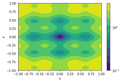
(a) Contour plot of the Bohachevsky function.

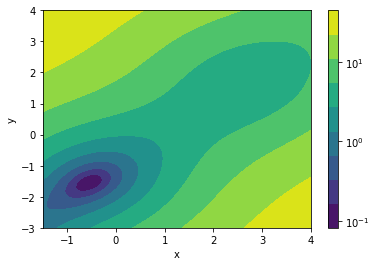
(b) Contour plot of the McCormick function.

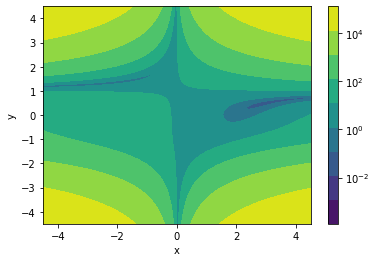
(c) Contour plot of the Beale function.

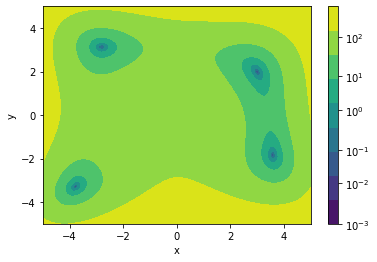
(d) Contour plot of the Himmelblau function.

Figure 1: Contour plots of our selected functions.

Function	Definition	Global minimum
Bohachevsky	$x^{2}+2y^{2}-.3\cos(3\pi x)-.4\cos(4\pi y)+.7$	$(0,0)$
McCormick	$\sin(x+y)+(x-y)^{2}-1.5x+2.5y+1$	None
Beale	$(1.5-x+xy)^{2}+(2.25-x+xy^{2})+(2.625-x+xy^{3})^{2}$	$(3,.5)$
Himmelblau	$(x^{2}+y-11)^{2}+(x+y^{2}-7)^{2}$	(3,2)

Table 1: Definitions of our selected functions.

The Bohachevsky function is characterized with an overall bowl shape which has a global minimum at $(0,0)$. However, this function has numerous local minima at intervals of approximately $.61$ in the $x$ direction and $.46$ in the $y$ direction, making it very easy for optimization algorithms to get stuck in a local minimum. The McCormick is a plate-shaped function, with no global minimum but many local minima at intervals of approximately $(\pi,\pi)$ of each other. These local minima have progressively smaller objective values as $x$ and $y$ approach $-\infty$. The usual search interval of this function is $-1.5\leq x\leq 4,-3\leq y\leq 4$, over which the minimum is $(-.54719,-1.54719)$. The Beale function has a cross-shaped valley, with peaks in the corners of the $x,y$-plane. Finally, the Himmelblau function is a bowl-shaped function, with four local minima: $(3,2),(-2.805118,3.131312),(-3.779310,-3.283186),$ and $(3.584428,-1.848126)$. Out of these, $(3,2)$ is the global minimum.

4.2 Newton Fractals

In this section, we present the second-order and third-order Newton fractals for each of these functions. One will observe that the third-order fractals display less sensitivity to the initial point, as well as wider basins of attraction.

Figures 2 and  3 contain the Newton fractals for the Bohachevsky function.

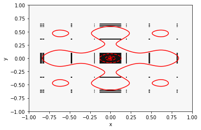
Figure 2: The second-order Newton fractal for the Bohachevsky function. Black regions indicate which initial points converge to the global minimum.

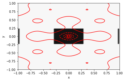
Figure 3: The third-order Newton fractal for the Bohachevsky function. Black regions indicate which initial points converge to the global minimum.

The fractals for the Bohachevsky function can overall be characterized by rectangular regions each containing a local minimum. Relatively speaking, the global minimum has a significantly larger basin of attraction for the third-order method than it does for the second-order method. Moreover, the second-order method contains many more noncontiguous initial iterates that converge to the global minimum. However, given that these points are closer to a separate local minimum, we consider this undesirable behavior.

Figures 4 and  5 contain the Newton fractals for the McCormick function.

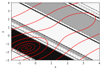
Figure 4: The second-order Newton fractal for the McCormick function. Black regions indicate which initial points converge to the global minimum in this region at $(-.54719,-1.54719)$, and grey regions indicate which initial points converge to the other local minimum at $(2.5944,1.5944)$.

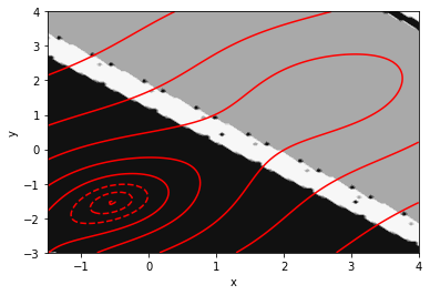
Figure 5: The third-order Newton fractal for the McCormick function. Black regions indicate which initial points converge to the global minimum in this region at $(-.54719,-1.54719)$, and grey regions indicate which initial points converge to the other local minimum at $(2.5944,1.5944)$.

The fractals for the McCormick function can be characterized by diagonal bands each containing a local minimum. Relatively speaking, the bands for the third-order method are wider, and the fractal contain fewer isolated thinner bands throughout.

Figures 6 and  7 contain the Newton fractals for the Beale function.

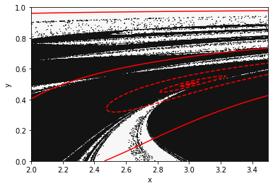
Figure 6: The second-order Newton fractal for the Beale function. Black regions indicate which initial points converge to the global minimum.

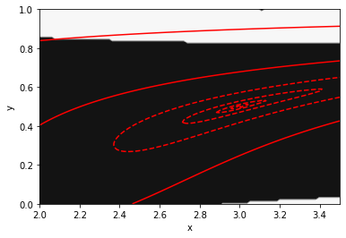
Figure 7: The third-order Newton fractal for the Beale function. Black regions indicate which initial points converge to the global minimum.

The fractal for the second-order method demonstrates very fractal behavior, with many iterates converging to a saddle point located at $(0,1)$. By comparison, the third-order fractal displays very stable behavior, with the basin of attraction being a contiguous region around the global minimum.

Figures 8 and  9 contain the Newton fractals for the Himmelblau function.

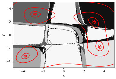
Figure 8: The second-order Newton fractal for the Himmelblau function. Differently colored regions indicate which initial points converge to the same local minimum.

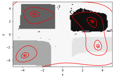
Figure 9: The third-order Newton fractal for the Himmelblau function. Differently colored regions indicate which initial points converge to the same local minimum.

Both fractals demonstrate the same overall behavior. Each local minimum has a contiguous region around it in which all points converge to it. However, both fractals have cross-shaped region in the middle of the local minima which have points that do not converge to any local minima. For the case of the second-order method, this cross-shaped region also contains extremely fractal behavior in the center. Compared to the second-order method, the cross-shaped region between the local minima for the third-order method is narrower and does not contain this fractal center, but the basin of attraction for each local minimum is also smaller.

4.3 Comparison Tests

Tables (2)-(5) contain the iteration count for each function for different algorithms and initial conditions.

Method	$(.1,.05)$	$(-.1,.02)$	$(.15,0)$	$(0,-.05)$
Second Order Newton	4	4	4	4
Third Order Newton	4	4	4	4
Quadratic Fit	15	13	4	4
Gradient Descent $c=0.05$	$\geq$4000	$\geq$4000	14	$\geq$4000
Gradient Descent $c=0.01$	39	39	41	13
Gradient Descent $c=0.015$	24	24	25	4
Gradient Descent $c=0.02$	17	17	17	13

Table 2: Numbers of iterations to converge to the global minimum for different algorithms and starting points for the Bohachevsky function.

Method	$(0,-1)$	$(-3,1)$	$(2,-3)$	$(2,-4)$
Second Order Newton	5	3	5	3
Third Order Newton	4	3	4	3
Quadratic Fit	5	9	11	4
Gradient Descent $c=0.2$	29	23	29	23
Gradient Descent $c=0.25$	22	18	22	18
Gradient Descent $c=0.3$	17	14	17	14
Gradient Descent $c=0.35$	14	17	17	17

Table 3: Numbers of iterations to converge to the global minimum for different algorithms and starting points for the McCormick function.

Method	$(2.8,.2)$	$(3,.2)$	$(3.2,.4)$	$(3.4,.3)$
Second Order Newton	8	7	6	7
Third Order Newton	7	7	4	7
Quadratic Fit	22	207	364	250
Gradient Descent $c=0.045$	$\geq$5000	$\geq$5000	$\geq$5000	$\geq$5000
Gradient Descent $c=0.035$	822	762	758	762
Gradient Descent $c=0.02$	1439	1321	1451	1605
Gradient Descent $c=0.01$	2880	2631	2913	3230

Table 4: Numbers of iterations to converge to the global minimum for different algorithms and starting points for the Beale function.

Method	$(2,1)$	$(4,1.5)$	$(4,3)$	$(3,3.5)$
Second Order Newton	7	5	4	5
Third Order Newton	4	3	3	3
Quadratic Fit	16	17	18	13
Gradient Descent $c=0.02$	21	24	27	27
Gradient Descent $c=0.015$	27	27	24	19
Gradient Descent $c=0.025$	$\geq$4000	$\geq$4000	$\geq$4000	$\geq$4000

Table 5: Numbers of iterations to converge to the global minimum for different algorithms and starting points for the Himmelblau function.

The overall relative behavior of the different algorithms was the same for each function. The Newton methods took the fewest iterations overall, with gradient descent with quadratic fit performing comparably on some initial points. Gradient descent with fixed step size took the most iterations overall on every function and initial point. Moreover, gradient descent with fixed step size was extremely sensitive to the chosen step size, not converging for many other choices thereof.

5 Levenberg-Marquardt Regularization for the Third-Order Method

From running our experiments, a main drawback of Algorithm 1 was that the SDP was often infeasible, especially when the current iterate was far from a local minimum. In this section, we investigate a generalization of Levenberg-Marquardt regularization which alleviates this problem.

5.1 Overview

In Levenberg-Marquardt regularization for the classical Newton’s method for nonconvex functions, a multiple of the identity matrix is added to the Hessian matrix in order to make the matrix positive definite. With this adjusted Hessian, the quadratic approximation now is guaranteed to have a global minimum.

A similar approach seems to be effective for the case of the third-order method. To motivate this with an example, we investigated an adjustment made to Algorithm 1 for the Himmelblau function. If the SDP (6) was infeasible, a multiple of the identity matrix added to the matrix $Q$ (see Figure 10). While the infeasibility issue was not completely resolved, one can see that all the basins of attraction increase in size as the multiple of the identity matrix increases. The question of interest then becomes whether there is a way to systematically decide what multiple of the identity matrix to add. For the second-order method, this is some constant which is at least the absolute value of the most negative eigenvalue of the Hessian matrix. For the third-order method it is not as obvious.

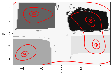
Figure 10: The third-order Newton fractal for the Himmelblau function, but with $5I$ (left) or $10I$ (right) added to the Hessian in the case of an infeasible SDP. Differently colored regions indicate which initial points converge to the same local minimum.

We point out that the our approach differs in a key aspect from existing algorithms. The idea of of adding a sufficiently large and convex function to an approximation is not new, but in existing algorithms this added function is at least on the order of the highest terms in the approximation. This is with the goal of making the approximation globally convex, guaranteeing that it has a global minimum and making it amenable to convex optimization techniques.

Here, the term we are adding is of lower order than that of the highest term in the approximation, as adding a multiple of the identity matrix to the Hessian is equivalent to adding a multiple of $\|x-x^{k}\|^{2}$ to the approximation. Such an adjustment will not make the approximation convex or introduce a global minimum, but it can induce a local minimum. Moreover, the same semidefinite program will find this local minimum, precluding the need for other more specialized techniques.

5.2 Choosing a scaling constant

In this section, we propose the following multiplier for the identity matrix. Let $\lambda$ be the minimum eigenvalue of $\triangledown^{2}f(x)$ and

$$g\mathrel{\mathop{:}}=\left[\begin{matrix}|\triangledown_{1}f(x)|\\ \vdots\\ |\triangledown_{n}f(x)|\end{matrix}\right],h\mathrel{\mathop{:}}=\left[\begin{matrix}\|\triangledown_{1}^{3}f(x)\|\\ \vdots\\ \|\triangledown_{n}^{3}f(x)\|\end{matrix}\right].$$

Then our choice of $\alpha$ is

$$\alpha_{LM}\mathrel{\mathop{:}}=\sqrt{\frac{3}{2}(\|g\|\|h\|+g^{T}h)}-\min\{0,\lambda\}.$$ (14)

Proposition 5.1.

For a three-times differentiable function $f$ and any point $\bar{x}\in\mathbb{R}^{n}$, the function $\Phi_{f,\bar{x}}+\alpha_{LM}\|x-\bar{x}\|^{2}$ has a local minimum.

Proof.

Recall from the proof of Theorem 3.1 that if the function

$$\delta(x,d)\mathrel{\mathop{:}}=b(x,d)^{2}-3a(x,d)c(x,d)$$ (15)

as defined in the proof is positive for all $d\neq 0$, then the Taylor expansion of $f$ around $x$ has a local minimum. If for some $\alpha\in\mathbb{R}$, $\triangledown^{2}f(x)$ is replaced by $\triangledown^{2}f(x)+\alpha I$, then this expression becomes

$$(b(x,d)+\alpha d^{T}d)^{2}-3a(x,d)c(x,d).$$ (16)

Since this function is still homogeneous with respect to $d$, we can consider whether this function is positive on $\|d\|=1$. If we can find $\beta$ such that $a(x,d)c(x,d)\leq\beta,\forall\|d\|=1$, then we can set

$$\alpha=\sqrt{3\beta}-\min\{0,\lambda\},$$ (17)

and satisfy (16). We point out that one natural choice of $\beta$ is $\|\triangledown^{3}p(x)\|\|\triangledown p(x)\|$, but it is NP-hard to compute the norm of the tensor $\triangledown^{3}p(x)$ [6]. Instead, for the rest of the proof we establish that

$$\beta=\frac{\|g\|\|h\|+g^{T}h}{2}$$ (18)

is a valid choice for $\beta$. Recall that $a(x,d)c(x,d)=(\triangledown f(x)^{T}d)(\sum_{i=1}^{n}d_{i}(d^{T}\triangledown_{i}^{3}f(x)d))$. One can see that

$$|a(x,d)c(x,d)|=|(\triangledown f(x)^{T}d)(\sum_{i=1}^{n}d_{i}(d^{T}\triangledown_{i}^{3}f(x)d))|\leq(\sum_{i=1}^{n}|d_{i}|g_{i})(\sum_{i=1}^{n}|d_{i}|h_{i}).$$

Note that since we are considering all $\|d\|=1$, the final expression on the right hand side is maximized on the nonnegative orthant, and so we can reduce that expression to $(d^{T}g)(h^{T}d).$

Now observe that $(d^{T}g)(h^{T}d)=d^{T}(\frac{gh^{T}+hg^{T}}{2})d$, where $gh^{T}+hg^{T}$ is a rank-2 matrix with the following eigenvalue-eigenvector pairs:

$$\left(g^{T}h+\|g\|\|h\|,\frac{g}{\|g\|}+\frac{h}{\|h\|}\right)$$

$$\left(g^{T}h-\|g\|\|h\|,\frac{g}{\|g\|}-\frac{h}{\|h\|}\right)$$

To verify this, one can see that

$$\left(gh^{T}+hg^{T})\frac{g}{\|g\|}+\frac{h}{\|h\|}\right)= \frac{g}{\|g\|}h^{T}g+\frac{g}{\|h\|}h^{T}h+\frac{h}{\|g\|}g^{T}g+\frac{h}{\|h\|}g^{T}h$$

$$= \left(\frac{g}{\|g\|}+\frac{h}{\|h\|}\right)g^{T}h+\frac{\|g\|}{\|g\|}\|h\|g+\frac{\|h\|}{\|h\|}\|g\|h$$

$$= (g^{T}h+\|g\|\|h\|)\left(\frac{g}{\|h\|}+\frac{h}{\|h\|}\right)$$

The other pair can be shown analogously. Note that because $g$ and $h$ have nonnegative entries by definition, the larger of the two eigenvalues is $g^{T}h+\|g\|\|h\|$. Hence the bound on $\beta$ is established, which concludes the proof. ∎

5.3 A revised algorithm

Ultimately we arrive at the following algorithm:

Algorithm 2 Unregularized Third-Order Newton’s Method with Levenberg Marquardt Regularization

1:Input: A function $f$, threshold $\epsilon>0$

2:Initialize a point $x^{0}$, $k=0$

3:While $\|\triangledown f(x^{k})\|>\epsilon$

4: If $\Phi_{f,x^{k}}$ has a local minimum:

5:  Let $x^{k+1}$ be the local minimum of $\Phi_{f,x^{k}}$

6:  Set $k=k+1$

7: Else

8:  Let $x^{k+1}$ be the local minimum of $\Phi_{f,x^{k}}+\alpha_{LM}^{k}\|x-x^{k}\|^{2}$

9:  Set $k=k+1$

10:Output: $x^{k}$

We do point out however, that choosing $\alpha$ as in (14) is generally an overestimation in regards to what is needed to make (6) feasible. We are providing a sufficient condition for (16) to hold, which is itself only a sufficient condition for the cubic approximation to have a local minimum, which itself is only a sufficient condition for (6) to be feasible. A worthwhile question to consider would be whether scalings based on SDP duality or an infeasbility certificate for the initial SDP can be derived. Having a better provable bound would be an improvement, and having an exact bound would be ideal. If an exact bound is known, one does not have to waste computations testing whether the SDP is feasible, and instead add the regularization term immediately. If one attempts to use a version of this algorithm that always adds the regularization term without an exact bound, convergence issues commonly arise close to the local minimum.

Below is the Newton fractal for the Himmelblau function when using Algorithm 2:

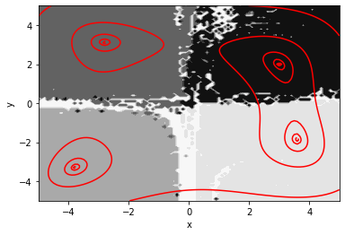
Figure 11: The third-order Newton fractal for the Himmelblau function with Levenberg Marquardt regularization. Differently colored regions indicate which initial points converge to the same local minimum.

As can be seen, when compared to the fractal in Figure 9, there is substantial improvement in the size of the basins of attraction, and a lessening of the locality of Algorithm 1. We do observe however that there are still starting iterates from which the algorithm diverges, or converges to a local minimum which is not the closest local minimum from the initial point. These are not issues that the Levenberg Marquardt regularization seeks to address.

6 Conclusion

In this paper, we presented a third-order unregularized Newton’s method, and showed guarantees on its performance along with some tests with optimistic results. Compared to the classical Newton’s method, the main advantage is the wider basins of attraction along with the reduced sensitivity to the initial point, as shown in the Newton fractals. From a time standpoint however, it is not competitive, provided that the second-order method converges. The main bottleneck of course is the cost of solving each intermediate SDP and the gain in iteration complexity not justifying the increased cost. The other main weakness of our algorithm is that the SDP we solve in each step is not always feasible. The quadratic Newton’s method on the other hand can still move to a saddle point as long as the Hessian has full rank. As the well-definedness of the next iterate provided in this work is local, so existence of this iterate is no longer guaranteed if the current iterate is far from the global minimum. This is especially true when the function being minimized is nonconvex.

General work on making SDP algorithms more efficient will improve the speed of our algorithm, but there is the potential of specific ways of working with our SDP. One change we believe is worth exploring is limiting the number of iterations that the SDP solver uses in each iteration of our Newton algorithm. It is unlikely that our algorithm requires a high degree of precision when generating iterates, and that finding a point close to the local minimum of each Taylor expansion is sufficient. Since the cubic function being minimized is only an approximation of the true function, it may be desirable to work with a new approximation as soon as possible. Such a modification could be considered a version of a damped Newton algorithm, and could be advantageous if our algorithm does not need optimal, or even near optimal solutions to the underlying SDPs to produce good iterations.

Overall, we believe that this work serves as a basis for a new class of third-order algorithms, and there are many avenues of further research in this direction. The most natural is to borrow on the literature on second-order Newton methods to improve our third-order method. While extending these methods to use third information are for the most part straightforward conceptually, there is the question of which adaptations will still result in computationally tractable subproblems. For example, the adaptation we presented in Section 5 can be viewed as an extension of Levenberg-Marquardt regularization, and does not require a change to the SDP. Damping can also be emulated, by using the SDP to find a direction, and then reducing the step size. Other adaptations, such as trust region approaches, may be less immediate, as minimizing a cubic polynomial over a sphere is an NP-hard problem [10].

References

- [1] E. P. Adorio and R. January. MVF - multivariate test functions library in C for unconstrained global optimization. 2005.
- [2] A. A. Ahmadi and J. Zhang. Complexity aspects of local minima and related notions. Advances in Mathematics, 397:108119, 2022.
- [3] S. Bubeck, Q. Jiang, Y. T. Lee, Y. Li, and A. Sidford. Near-optimal method for highly smooth convex optimization. In Conference on Learning Theory, pages 492–507. PMLR, 2019.
- [4] A. Conn, N. Gould, and P. Toint. Trust Region Methods. MPS-SIAM Series on Optimization. Society for Industrial and Applied Mathematics, 2000.
- [5] A. Gasnikov, P. Dvurechensky, E. Gorbunov, E. Vorontsova, D. Selikhanovych, and C. A. Uribe. Optimal tensor methods in smooth convex and uniformly convex optimization. In Conference on Learning Theory, pages 1374–1391. PMLR, 2019.
- [6] C. J. Hillar and L.-H. Lim. Most tensor problems are NP-hard. Journal of the ACM (JACM), 60(6):1–39, 2013.
- [7] K. Levenberg. Method for the solution of certain problems in least squares. J Numer Anal, 16:588–A604, 1944.
- [8] D. W. Marquardt. An algorithm for least-squares estimation of nonlinear parameters. Journal of the society for Industrial and Applied Mathematics, 11(2):431–441, 1963.
- [9] J. J. Moré. Recent developments in algorithms and software for trust region methods. In ISMP, 1982.
- [10] J. E. Nesterov et al. Random walk in a simplex and quadratic optimization over convex polytopes. Technical report, CORE, 2003.
- [11] Y. Nesterov. Implementable tensor methods in unconstrained convex optimization. Mathematical Programming, 186(1):157–183, 2021.
- [12] Y. Nesterov and B. T. Polyak. Cubic regularization of newton method and its global performance. Mathematical Programming, 108(1):177–205, 2006.
- [13] J. M. Ortega and W. C. Rheinboldt. Iterative solution of nonlinear equations in several variables. SIAM, 2000.
- [14] M. J. D. Powell. A new algorithm for unconstrained optimization. 1970.
- [15] L. Vandenberghe and S. Boyd. Semidefinite programming. SIAM Review, 38(1):49–95, 1996.