Contractivity of the Method of Successive Approximations
for Optimal Control

Abstract

Strongly contracting dynamical systems have numerous properties (e.g., incremental ISS), find widespread applications (e.g., in controls and learning), and their study is receiving increasing attention. This work starts with the simple observation that, given a strongly contracting system, its adjoint dynamical system is also strongly contracting, with the same rate, with respect to the dual norm, under time reversal. As main implication of this dual contractivity, we show that the classic Method of Successive Approximations (MSA), an indirect method in optimal control, is a contraction mapping for short optimization intervals or large contraction rates. Consequently, we establish new convergence conditions for the MSA algorithm, which further imply uniqueness of the optimal control and sufficiency of Pontryagin’s minimum principle under additional assumptions.

1 Introduction

Optimal control is generally a difficult problem, and with the exception of some analytically tractable cases, it must be solved numerically. Numerical approaches broadly fall into two categories: direct and indirect methods. Direct methods, like direct collocation and direct shooting methods [23, 22, 3], discretize and approximate the state and/or control to encode the problem as a nonlinear program. Due to their relative simplicity, robustness, and the wide availability of software implementations, direct methods tend to be favored in modern times [3, §4.3], [8].

Indirect methods are an older class of methods based on Pontryagin’s minimum principle (PMP), which gives a necessary condition for optimality of a control signal. PMP states that the optimal trajectory must solve a two-point boundary problem, together with a costate, and that the optimal control minimizes a Hamiltonian function at each point in time. Indirect methods search for an input, state trajectory, and costate trajectory that satisfy PMP. Many direct methods, including shooting and collocation, can also be applied as indirect methods to the PMP boundary value problem [12]. Another approach is the Method of Successive Approximations (MSA) [7], also called the Forward-Backward-Sweep algorithm [17], which is the main topic of this letter.

MSA [13, 16, 1] and its variants [21, 7] are classic approaches that have received renewed attention in the machine learning community [19, 18, 4] as alternatives to gradient descent for training residual neural networks (ResNets). Indeed, a new thrust of machine learning research is to apply control-theoretic techniques to the training of ResNets by viewing these models as forward Euler discretizations of continuous-time control systems [10, 25, 24]. Within this framework, training the ResNet can be viewed as an optimal control problem. As argued in [19, 18], MSA (and its variants) allow for error and convergence analysis and can lead to better training dynamics than gradient descent.

Unfortunately, MSA does not always converge, a problem that is still the subject of ongoing research. In [20], the authors prove convergence criteria based on boundedness and Lipschitz assumptions. Similar bounds are established in [19, 18]. This letter provides a new set of convergence criteria when MSA is applied to strongly contracting dynamical systems.

The contributions of this letter are as follows. First, in §3, we study the adjoints of nonlinear systems that arise in optimal control theory. We show that adjoints of contracting systems under time reversal are also contracting with the same rate, albeit with respect to the dual norm. This property allows us to prove Grönwall-like and ISS-like bounds on the adjoint dynamics. §4 applies these bounds to analyze MSA. Assuming Lipschitz continuity of all relevant maps in the optimal control problem, we obtain a bound on the Lipschitz constant of each MSA iteration. This Lipschitz constant becomes arbitrarily small in the limits of short optimization intervals and large contraction rates, thereby establishing conditions for when the iteration is a contraction mapping. With an additional assumption of pointwise uniqueness of the minimizer of the Hamiltonian, we show that these conditions also lead to uniqueness of the optimal control and sufficiency of PMP. Finally, in §5, we provide an illustrative example.

2 Preliminaries

2.1 Contracting Dynamics over Normed Vector Spaces

Let $\lVert\cdot\rVert:{}^{n}\to{}_{\geq 0}$ be a norm. The dual norm $\lVert\cdot\rVert_{\star}:{}^{n}\to{}_{\geq 0}$ is the norm $\lVert x\rVert_{\star}=\sup_{\lVert y\rVert\leq 1}y^{\mathsf{T}}x$. Given a matrix $A\in{}^{n\times n}$, the induced norm of $A$ is $\lVert A\rVert=\sup_{\lVert x\rVert=1}\lVert Ax\rVert$ and the induced logarithmic norm of $A$ is

$$\mu(A)=\lim_{\alpha\to 0^{+}}\frac{\lVert I_{n}+\alpha A\rVert-1}{\alpha}.$$

Explicit formulas for the induced (logarithmic) norms are known for the standard $p\in\{1,2,\infty\}$ norms on ⁿ [6, §2.4].

A map $T:X\to Y$ between normed spaces $(X,\lVert\cdot\rVert_{X})$ and $(Y,\lVert\cdot\rVert_{Y})$ is Lipschitz continuous if a constant $\ell\geq 0$ exists such that $\lVert T(x)-T(\bar{x})\rVert_{Y}\leq\ell\lVert x-\bar{x}\rVert_{X}$ for all $x,\bar{x}\in X$. The minimal Lipschitz constant ${\rm Lip}(T)$ is the infimum over $\ell$ that satisfy this inequality. If $T$ is continuously differentiable, then ${\rm Lip}(T)=\sup_{x\in X}\lVert D_{x}T(x)\rVert$, where $D_{x}T(x)$ denotes the Jacobian matrix of $T$. Furthermore, if $X=Y={}^{n}$, then the one-sided Lipschitz constant of $T$ is ${\rm osL}(T)=\sup_{x\in X}\mu(D_{x}T(x))$. A dynamical system $\dot{x}=f(t,x,\dots)$ with a continuously differentiable vector field $f:{}^{n}\to{}^{n}$ is said to be strongly infinitesimally contracting with rate $c>0$ if the map $x\mapsto f(t,x,\dots)$ is uniformly one-sided Lipschitz with constant $-c$ for all $t$ and for all inputs.

Strongly contracting systems enjoy numerous properties. As a useful example, we state the following lemma without proof (as it slightly generalizes [6, Theorem 3.15, Corollary 3.16]).

Lemma 1 (Grönwall comparison lemma)

Consider a dynamical system

$$\dot{x}(t)=f(t,x(t),u_{1}(t),\dots,u_{m}(t)),\qquad\forall t\geq 0,$$ (1)

with $x(t)\in{}^{n}$ and inputs $u_{i}\in U_{i}\subseteq{}^{k_{i}}$ for $i\in\{1,2,\dots,m\}$. Let $\lVert\cdot\rVert$ be a norm on ⁿ, and let $\lVert\cdot\rVert_{U_{i}}$ be norms on $U_{i}$. Assume that

1. the system (1) is strongly infinitesimally contracting with rate $c>0$, and

2. for each $i\in\{1,2,\dots,m\}$, the maps $u_{i}\mapsto f(t,x,u_{1},\dots,u_{i},\dots,u_{m})$ are uniformly Lipschitz continuous with constant $\ell_{f,U_{i}}$ for all $t\geq 0$, $x\in{}^{n}$, and $u_{j}\in U_{j}$ with $j\neq i$.

Let $(u_{1},\dots,u_{m})$ and $(\bar{u}_{1},\dots,\bar{u}_{m})$ be input signals, and let $x,\bar{x}$ be the corresponding trajectories of (1). For all $t\geq 0$,

$$\begin{split}&\lVert x(t)-\bar{x}(t)\rVert\leq e^{-ct}\lVert x(0)-\bar{x}(0)\rVert\\ &\qquad+\sum_{i=1}^{m}\ell_{f,U_{i}}\int_{0}^{t}e^{-c(t-\tau)}\lVert u_{i}(\tau)-\bar{u}_{i}(\tau)\rVert_{U_{i}}d\tau.\end{split}$$ (2)

Note that (2) still holds when $c\leq 0$, i.e., for expansive systems with a bounded rate of expansion; however, we do not consider such systems in this letter.

2.2 Optimal Control

We study the following optimal control problem:

Problem 1 (Optimal control problem)

Consider a dynamical system

$$\dot{x}(t)=f(t,x(t),u(t)),\quad x(0)=x_{0}\in{}^{n},$$ (3)

where $f$ is continuous in all arguments and continuously differentiable in the second and third arguments. Further consider a cost functional

$$J[u]=\int_{0}^{T}\phi(t,x(t),u(t))\,dt+\psi(x(T)),$$ (4)

where $\phi:[0,T]\times{}^{n}\times U\to\real$ is a running cost that is differentiable in the second argument, and $\psi:{}^{n}\to\real$ is a differentiable terminal cost. Let $\mathcal{U}=\left\{u:[0,T]\to U~{}\text{s.t.}~{}u~{}\text{measurable}\right\}$ be a space of permissible control signals, where $T>0$ and $U\subseteq{}^{k}$ is a compact set containing $\mathbbold{0}_{k}$. The optimal control problem is to find $u^{*}\in\mathcal{U}$ that minimizes $J[u^{*}]$.

An elementary necessary condition for the optimality of a control is Pontryagin’s minimum principle (PMP) [2, Theorem 5.10, Theorem 5.11] [5, Theorem 6.3.1, Theorem 6.5.1]:

Theorem 2 (Pontryagin’s minimum principle)

Let $u^{*}\in\mathcal{U}$ be an optimal control for Problem 1 (if one exists), and let $x:[0,T]\to{}^{n}$ be the corresponding trajectory of (3). For all $t\in[0,T]$,

$$u^{*}(t)\in\operatorname*{argmin}_{\tilde{u}\in U}H(t,x(t),\lambda(t),\tilde{u}),$$ (5)

where $H:\real\times{}^{n}\times{}^{n}\times U\to\real$ is the Hamiltonian

$$H(t,x,\lambda,u)=\lambda^{\mathsf{T}}f(t,x,u)+\phi(t,x,u)$$ (6)

and $\lambda:[0,T]\to{}^{n}$ is the costate trajectory

$$\dot{\lambda}(t)=-D_{x}f(t,x(t),u(t))^{\mathsf{T}}\lambda(t)-\phi_{x}(t,x(t),u(t))$$ (7)

with the boundary condition $\lambda(T)=\psi_{x}(x(T))$.

2.3 Method of Successive Approximations

The Method of Successive Approximations (MSA) [7], also called the Forward-Backward Sweep algorithm [17], is a basic approach to computing an input that satisfies PMP. The method iteratively solves the PMP two-point boundary value problem, then updates the control to minimize the new Hamiltonian at each time, as outlined in Algorithm 1.

Algorithm 1 Method of Successive Approximations

0:  initial guess $u^{(0)}\in\mathcal{U}$

1:  for $i=1,2,\dots,N$ :

2:        $x^{(i)}\leftarrow$ trajectory of (3) from $x_{0}$ with input $u^{(i-1)}$

3:        $\lambda^{(i)}\leftarrow$ trajectory of (7) from $\lambda(T)=\psi_{x}(x^{(i)}(T))$ with inputs $x^{(i)}$ and $u^{(i-1)}$

4:        $u^{(i)}(t)\leftarrow\operatorname*{argmin}_{\tilde{u}\in U}H(t,x^{(i)}(t),\lambda^{(i)}(t),\tilde{u})$ for all $t\in[0,T]$, ties broken arbitrarily

5:  return  $u^{(N)}$

The algorithm can run for a fixed number of iterations; alternatively, it may terminate when the difference between successive iterates $u^{(i-1)}$, $u^{(i)}$ is within a specified tolerance. Note that each iteration of the algorithm maps a control $u^{(i-1)}$ to a new control $u^{(i)}$, so that each iteration can be thought of as an operator $\operatorname{MSA}:\mathcal{U}\to\mathcal{U}$.

Definition 3 (MSA Operator)

Given a control $u\in\mathcal{U}$, let $x:[0,T]\to{}^{n}$ be the corresponding trajectory of (3), and let $\lambda:[0,T]\to{}^{n}$ be the trajectory of (7) from $\lambda(T)=\psi_{x}(x(T))$. Then $\operatorname{MSA}(u)$ is the control that satisfies (5) with respect to $x(t)$ and $\lambda(t)$ for all $t\in[0,T]$, with ties broken in an arbitrary deterministic manner.

Definition 3 is well-posed if the signal of Hamiltonian-minimizing controls from (5) is measurable. When we analyze the MSA algorithm in §4, we will impose Lipschitz continuity assumptions that forbid any edge cases where $\operatorname{MSA}(u)$ is not measurable.

2.4 Adjoints

Adjoints are familiar from linear systems theory. Given input and output Hilbert spaces $\mathcal{S}_{\rm in},\mathcal{S}_{\rm out}$ and a linear system $G:\mathcal{S}_{\rm in}\to\mathcal{S}_{\rm out}$, the adjoint of $G$ is the unique linear system $\tilde{G}:\mathcal{S}_{\rm out}\to\mathcal{S}_{\rm in}$ such that $\langle Gu,y\rangle_{\mathcal{S}_{\rm out}}=\langle u,\tilde{G}y\rangle_{\mathcal{S}_{\rm in}}$ for all $u\in\mathcal{S}_{\rm in}$ and $y\in\mathcal{S}_{\rm out}$. For an LTV system with the usual $(A,B,C,D)$ representation, the adjoint dynamics are

$$\dot{\lambda}(t) =-A(t)^{\mathsf{T}}\lambda(t)-C(t)^{\mathsf{T}}v(t)$$ (8a)

$$z(t) =B(t)^{\mathsf{T}}\lambda(t)+D(t)^{\mathsf{T}}v(t)$$ (8b)

with $v\in\mathcal{S}_{\rm out}$ and $z\in\mathcal{S}_{\rm in}$ [11, 3.2.4]. The theory of adjoints leads to the duality of controllability and observability and of linear quadratic regulators and estimators [15].

3 Contractivity of the Adjoint

This section examines adjoints of nonlinear systems. We first explain how the notion of “adjoint” frequently used in the optimal control literature relates to the adjoint from linear systems. We then prove a simple yet powerful result: that the adjoint of a strongly infinitesimally contracting system is itself strongly infinitesimally contracting, with respect to the dual norm, when integrated backwards in time. This dual contractivity property leads to useful bounds for the evolution of costates, to later be employed in §4.

3.1 Adjoints of Nonlinear Systems

Nonlinear systems do not properly have adjoints according to the definition in §2.4. Instead, the adjoint of the system’s linearized variational dynamics is often referred to as its adjoint [13, 9]. Consider the nonlinear system (3) with output $y(t)=x(t)$. Let $u(t)$ be an input signal corresponding to a nominal trajectory $x(t)$, let $\tilde{x}(t)$ be the trajectory from $\tilde{u}(t)$. Linearizing the dynamics of $\delta x(t)=\tilde{x}(t)-x(t)$ from $\delta u(t)=\tilde{u}(t)-u(t)$,

$$\dot{(\delta x)}(t) =D_{x}f(t,x(t),u(t))\delta x(t)+D_{u}f(t,x(t),u(t))\delta u(t)$$

$${(\delta y)(t)} =\delta x(t)$$

so by (8a), the adjoint dynamics are

$$\dot{\lambda}(t) =-D_{x}f(t,x(t),u(t))^{\mathsf{T}}\lambda(t)-v(t)$$ (9a)

$$z(t) =D_{u}f(t,x(t),u(t))^{\mathsf{T}}\lambda(t)$$ (9b)

where $v(t)\in V\subseteq{}^{n}$. Not coincidentally, the costate dynamics (7) from PMP are of the form (9a), with a forcing term $v(t)=\phi_{x}(t,x(t),u(t))$ from the running cost. Indeed, PMP can be derived from the variational linearization described above; see [5, Theorem 2.3.1, Theorem 6.1.1].

3.2 Contractivity of the Adjoint

We now examine the adjoints of strongly contracting systems. When the original system is contracting with respect to a norm $\lVert\cdot\rVert$, it is natural to study the adjoint system using the dual norm $\lVert\cdot\rVert_{\star}$, as the following lemma suggests.

Lemma 4 (Dual Lipschitz constants)

Let $\lVert\cdot\rVert:{}^{n}\to{}_{\geq 0}$ be a norm, and let $\lVert\cdot\rVert_{\star}$ be its dual norm. Let $f,g:{}^{n}\to{}^{n}$ be a pair of continuously differentiable vector fields, such that $D_{x}f(x)=D_{x}g(x)^{\mathsf{T}}$ for all $x\in{}^{n}$. Then

1. ${\rm Lip}_{\lVert\cdot\rVert}(f)={\rm Lip}_{\lVert\cdot\rVert_{\star}}(g)$, and

2. ${\rm osL}_{\lVert\cdot\rVert}(f)={\rm osL}_{\lVert\cdot\rVert_{\star}}(g)$.

The following is an immediate consequence of Lemma 4:

Theorem 5 (Dual contraction)

Consider the pair of dynamical systems (3) and (9a). Let $T>0$ and $c>0$, let $\lVert\cdot\rVert$ be a norm on ⁿ, and let $\lambda^{\leftarrow}(t)=\lambda(T-t)$ be the time-reversed trajectory of (9a) (where we study the time-reversed dynamics due to the minus sign in the vector field). The following are equivalent:

1. the $x(t)$ system is strongly infinitesimally contracting with respect to $\lVert\cdot\rVert$ with rate $c$, and

2. the $\lambda^{\leftarrow}(t)$ system is strongly infinitesimally contracting with respect to $\lVert\cdot\rVert_{\star}$ with rate $c$.

Proof 3.6.

Let $g$ be the function

$$g(t,\tilde{\lambda},\tilde{x},\tilde{u})\triangleq\frac{d\lambda^{\leftarrow}(t)}{dt}=D_{x}f(t,\tilde{x},\tilde{u})^{\mathsf{T}}\tilde{\lambda}+v(t),$$

For all fixed $t$, $\tilde{\lambda}$, $\tilde{x}$, and $\tilde{u}$, we have $D_{\lambda}g(t,\tilde{\lambda},\tilde{x},\tilde{u})=D_{x}f(t,\tilde{x},\tilde{u})^{\mathsf{T}}$. Hence, applying Lemma 4 to the maps $\tilde{g}(\lambda)=g(t,\lambda,\tilde{x},\tilde{u})$ and $\tilde{f}(x)=f(t,x,\tilde{u})$, we obtain ${\rm osL}_{\lVert\cdot\rVert}(\tilde{f})={\rm osL}_{\lVert\cdot\rVert_{\star}}(\tilde{g})$. Thus the maps $\lambda=g(t,\lambda,\tilde{x},\tilde{u})$ are uniformly one-sided Lipschitz with constant $-c$ with respect to $\lVert\cdot\rVert_{\star}$, if and only if the maps $x\mapsto f(t,x,\tilde{u})$ have the same property with respect to $\lVert\cdot\rVert$.

3.3 Bounds on Adjoint Dynamics

Theorem 5 establishes that $\lambda^{\leftarrow}(t)$ is strongly contracting so long as the original system is strongly contracting, so we can exploit standard bounds on contracting systems to bound the evolution of $\lambda(t)$. Before stating these bounds, we impose the following two assumptions:

Assumption 1 (Strong contractivity)

The system (3) is strongly infinitesimally contracting with rate $c>0$, i.e., ${\rm osL}(f(t,\tilde{x},\tilde{u}))\leq-c$ for all $t\in[0,T]$ and $\tilde{u}\in U$. Furthermore, the trajectory of (3) on the interval $[0,T]$ with $u(t)=\mathbbold{0}_{k}$ is bounded.

Assumption 2 (Lipschitz continuity, Pt. I)

For all fixed $t\in[0,T]$ and $x\in{}^{n}$, the map $u\mapsto f(t,\tilde{x},u)$ from $({}^{k},\lVert\cdot\rVert_{U})$ into $({}^{n},\lVert\cdot\rVert)$ is Lipschitz with constant $\ell_{f,u}$.

Strong contractivity is a fairly strong assumption. For example, if some $x^{*}\in{}^{n}$ is an equilibrium point of the unforced system for all $t$, strong contractivity implies that $x^{*}$ is globally exponentially stable (due to Lemma 1). Due to Theorem 5, the assumption also implies that the adjoint dynamics are also strongly contracting. Consequently, we can prove that all state and costate trajectories remain bounded.

Lemma 3.7 (Boundedness of state and costate).

Consider the system (3) and its adjoint (7). If the input spaces $U\subset({}^{k},\lVert\cdot\rVert_{U})$ and $V\subset({}^{n},\lVert\cdot\rVert_{\star})$ are bounded, then under Assumptions 1 and 2, there exist bounded sets $X\subset({}^{n},\lVert\cdot\rVert)$ and $\Lambda\subset({}^{n},\lVert\cdot\rVert_{\star})$ such that $x(t)\in X$ and $\lambda(t)\in\Lambda$ for all $t\in[0,T]$ and measurable $u:[0,T]\to U$ and $v:[0,T]\to V$.

In the remainder of this letter, we will let $X,\Lambda\subset{}^{n}$ be the bounded sets guaranteed by Lemma 3.7. In particular, the boundedness of $\lambda(t)$ allows us to impose additional Lipschitz continuity assumptions:

Assumption 3 (Lipschitz continuity, Pt. II)

For all fixed $t\in[0,T]$, $\tilde{x}\in X$, $\tilde{u}\in U$, and $\tilde{\lambda}\in\Lambda$,

1. the map $x\mapsto D_{x}f(t,x,\tilde{u})^{\mathsf{T}}\tilde{\lambda}$ from $({}^{n},\lVert\cdot\rVert)$ into $({}^{n},\lVert\cdot\rVert_{\star})$ is Lipshitz with constant $\ell_{f_{x},x}$, and

2. the map $u\mapsto D_{x}f(t,\tilde{x},u)^{\mathsf{T}}\tilde{\lambda}$ from $({}^{k},\lVert\cdot\rVert_{U})$ into $({}^{n},\lVert\cdot\rVert_{\star})$ is Lipschitz with constant $\ell_{f_{x},u}$.

We are now ready to state the first bound on the evolution of the adjoint trajectories.

Theorem 3.8 (Grönwall comparison of costates).

Consider the system (3) and its adjoint (9a) with Assumptions 1–3. Let $u,\bar{u}:[0,T]\to U$ and $v,\bar{v}:[0,T]\to V$ be two pairs of measurable input signals, and let $\lambda,\bar{\lambda}:[0,T]\to{}^{n}$ be the corresponding adjoint trajectories. Then for all $t\geq 0$,

$$\begin{split}&\lVert\lambda(t)-\bar{\lambda}(t)\rVert_{\star}\leq e^{-c(T-t)}\lVert\lambda(T)-\bar{\lambda}(T)\rVert_{\star}\\ &\;\;\;\;+\int_{t}^{T}e^{-c(\tau-t)}\lVert v(\tau)-\bar{v}(\tau)\rVert_{\star}\,d\tau\\ &\;\;\;\;+\ell_{f_{x},u}\int_{t}^{T}e^{-c(\tau-t)}\lVert u(\tau)-\bar{u}(\tau)\rVert_{U}\,d\tau\\ &\;\;\;+\frac{\ell_{f_{x},x}\ell_{f,u}\sinh(c(T\!-\!t))}{c}\!\!\;\int_{0}^{t}\!\!\!e^{-c(T-\tau)}\lVert u(\tau)\!-\!\bar{u}(\tau)\rVert_{U}\,d\tau\\ &\;\;\;+\frac{\ell_{f_{x},x}\ell_{f,u}e^{-c(T-t)}}{c}\!\!\int_{t}^{T}\!\!\!\!\sinh(c(T\!-\!\tau))\lVert u(\tau)\!-\!\bar{u}(\tau)\rVert_{U}\,d\tau.\end{split}$$ (10)

Theorem 3.8 provides a somewhat unwieldy bound. We can sacrifice its sharpness to obtain a much simpler incremental ISS property.

Corollary 3.9 (Incremental ISS of adjoint systems).

Under the same hypotheses as Theorem 3.8,

$$\begin{split}&\sup_{t\in[0,T]}\lVert\lambda(t)-\bar{\lambda}(t)\rVert_{\star}\leq\lVert\lambda(T)-\bar{\lambda}(T)\rVert_{\star}\\ &\qquad\;\;+\kappa\sup_{t\in[0,T]}\lVert v(t)-\bar{v}(t)\rVert_{\star}\\ &\qquad\;\;+\left(\ell_{f_{x},u}\kappa+\ell_{f_{x},x}\ell_{f,u}\kappa^{2}\right)\sup_{t\in[0,T]}\lVert u(t)-\bar{u}(t)\rVert_{U}.\end{split}$$ (11)

where

$$\kappa=c^{-1}(1-e^{-cT}).$$ (12)

4 Applications to Optimal Control

Here we show how the contractivity of the adjoint system leads to the contractivity of the MSA iteration, under additional Lipschitz continuity assumptions.

Assumption 4 (Lipschitz continuity of cost gradients)

For all fixed $t\in[0,T]$, $\tilde{x}\in X$, and $\tilde{u}\in U$,

1. the map $x\mapsto\phi_{x}(t,x,\tilde{u})$ from $({}^{n},\lVert\cdot\rVert)$ into $({}^{n},\lVert\cdot\rVert_{\star})$ is Lipschitz with constant $\ell_{\phi_{x},x}$,

2. the map $u\mapsto\phi_{x}(t,\tilde{x},u)$ from $({}^{k},\lVert\cdot\rVert_{U})$ into $({}^{n},\lVert\cdot\rVert_{\star})$ is Lipschitz with constant $\ell_{\phi_{x},u}$, and

3. the map $x\mapsto\psi_{x}(x)$ from $({}^{n},\lVert\cdot\rVert)$ into $({}^{n},\lVert\cdot\rVert_{\star})$ is Lipschitz with constant $\ell_{\psi_{x},x}$.

Assumption 5 (Lipschitz continuity of the optimum)

There exists a continuous map $h:[0,T]\times X\times\Lambda\to U$ such that

$$h(t,x,\lambda)\in\operatorname*{argmin}_{u\in U}H(t,x,\lambda,u)$$ (13)

for all $t\in[0,T]$, $x\in X$, and $\lambda\in\Lambda$, with ties broken in an identical manner as the MSA operator, where for all fixed $t\in[0,T]$, $\tilde{x}\in X$, and $\tilde{\lambda}\in\Lambda$,

1. the map $x\mapsto h(t,x,\tilde{\lambda})$ from $({}^{n},\lVert\cdot\rVert)$ into $({}^{k},\lVert\cdot\rVert_{U})$ is Lipschitz with constant $\ell_{h,x}$, and

2. the map $\lambda\mapsto h(t,\tilde{x},\lambda)$ from $({}^{n},\lVert\cdot\rVert_{\star})$ into $({}^{k},\lVert\cdot\rVert_{U})$ is Lipschitz with constant $\ell_{h,\lambda}$.

Notice that Assumption 5 implies that $\operatorname{MSA}(u)$ is measurable for any $u\in\mathcal{U}$. With these Lipshitz assumptions, we can finally bound the Lipschitz constant of the MSA operator.

Theorem 4.10 (Contractivity of MSA).

Suppose that Problem 1 is nonsingular and satisfies Assumptions 1–5, and consider the norm $\lVert\cdot\rVert_{\mathcal{U}}:\mathcal{U}\to{}_{\geq 0}$ given by

$$\lVert u\rVert_{\mathcal{U}}=\sup_{t\in[0,T]}\lVert u(t)\rVert_{U}.$$ (14)

The following are true:

1. The Lipschitz constant of an MSA iteration with respect to the $\lVert\cdot\rVert_{\mathcal{U}}$ norm is bounded by

   $${\rm Lip}(\operatorname{MSA})\leq b_{1}\kappa+b_{2}\kappa^{2}$$ (15)

   where

   $$b_{1} =\ell_{h,x}\ell_{f,u}+\ell_{h,\lambda}\left(\ell_{\psi_{x},x}\ell_{f,u}+\ell_{\phi_{x},u}+\ell_{f_{x},u}\right)$$ (16a)

   $$b_{2} =\ell_{h,\lambda}\ell_{f,u}\left(\ell_{\phi_{x},x}+\ell_{f_{x},x}\right)$$ (16b)

2. If $b_{1}\kappa+b_{2}\kappa^{2}<1$, then the $\operatorname{MSA}$ operator is a contraction; hence it has a unique fixed point $\hat{u}\in\mathcal{U}$, the $\operatorname{MSA}$ iterates $u^{(i)}=\operatorname{MSA}^{i}(u^{(0)})$ converge to $\hat{u}$ from any initial guess $u^{(0)}\in\mathcal{U}$, and

   $$\lVert u^{(i)}(t)-\hat{u}(t)\rVert_{U}\leq\left(\frac{(b_{1}\kappa+b_{2}\kappa^{2})^{i}}{1-b_{1}\kappa-b_{2}\kappa^{2}}\right)\lVert u^{(1)}-u^{(0)}\rVert_{\mathcal{U}}$$

   for all $t\in[0,T]$.

Corollary 4.11 (Uniqueness and Sufficiency).

Under the same hypotheses as Theorem 4.10, if additionally

1. the Hamiltonian has a unique minimizer for all $t\in[0,T]$, $x\in X$, and $\lambda\in\Lambda$,

2. an optimal control $u^{*}$ exists, and

3. the time horizon $T$ is sufficiently small or the contraction rate $c$ is sufficiently large that ${\rm Lip}(\operatorname{MSA})<1$,

then $u^{*}$ is the unique optimal control, and PMP is a sufficient condition for optimality.

5 Example

Figure 1: Diagram of the nonlinear circuit studied in Section 5.

For an illustrative example the results, consider the circuit from [14, §1.2.2], depicted in Figure 1. The circuit contains a nonlinear resistive element, with a current-voltage relationship $i_{h}=r(v_{h})$ for some twice-differentiable function $r:\real\to\real$ with $r(0)=0$. We assume that $R>1$, that $r^{\prime}(x_{1})\geq 1+\epsilon$ for some $\epsilon>0$, and that $r^{\prime\prime}(x_{1})$ is bounded for all $x_{1}\in\real$. (This assumption allows us to use the $\mathcal{L}_{\infty}$ norm for simplified analysis; weighted norms can be used to generalize the parameter ranges.) The state variables are $x_{1}\in\real$ (voltage across the nonlinear element) and $x_{2}\in\real$ (current through the inductor), and the control input $u\in\real$ is the voltage across the source. The dynamics are

$$\dot{x}_{1}=\frac{1}{C}\left(-r(x_{1})+x_{2}\right),\quad\dot{x}_{2}=\frac{1}{L}\left(-x_{1}-Rx_{2}+u\right)$$

from an initial condition $x(0)=\mathbbold{0}_{2}$. Our objective is to minimize the cost

$$J[u]=\int_{0}^{T}\underbrace{\frac{1}{2}u^{2}(t)}_{\phi}\,dt+\underbrace{\frac{\gamma}{2}\lVert x(T)-x^{*}\rVert_{2}^{2}}_{\psi}$$

for some terminal cost weight $\gamma>0$, where $x^{*}\in{}^{2}$ is an arbitrary target state, and the space of permissible controls is $U=[-u_{\rm max},u_{\rm max}]$ for some $u_{\rm max}>0$. Note that $\mathbbold{0}_{2}$ is an equilibrium point of the unforced dynamics.

5.1 Examining the Assumptions

This optimal control problem satisfies Assumptions 1–5, as we demonstrate in the following paragraphs.

Assumption 1

The dynamics are strongly infinitesimally contracting with respect to the $\mathcal{L}_{\infty}$ norm:

$${\rm osL}(f) =\sup_{x\in{}^{2}}\mu_{\infty}(D_{x}f(x))$$

$$=\sup_{x_{1}\in\real}\max\left\{\frac{1-r^{\prime}(x_{1})}{C},\;\frac{1-R}{L}\right\}$$

$$=\max\left\{\frac{1-d_{\rm min}}{C},\;\frac{1-R}{L}\right\}\triangleq-c<0$$

where $d_{\rm min}=\inf_{x_{1}\in\real}r^{\prime}(x_{1})>1$. Thus Assumption 1 is satisfied with contraction rate $c$.

Assumption 2

Given two inputs $u,\bar{u}\in\real$, $\lVert f(x,u)-f(x,\bar{u})\rVert_{\infty}=L^{-1}|u-\bar{u}|$ for all $x\in{}^{2}$, so Assumption 2 is satisfied with $\ell_{f,u}=L^{-1}$.

Reachability Analysis

Before we examine Assumption 3, it is useful to bound the set of states that are reachable within time $T$. Lemma 1 allows us to compare $x(t)$ with the trajectory at the origin corresponding to zero input:

$$\lVert x(t)\rVert_{\infty}\leq L^{-1}\int_{0}^{t}e^{-c(t-\tau)}|u(\tau)|~{}d\tau\leq\frac{u_{\rm max}(1-e^{-ct})}{cL}$$

In particular, $x(T)$ belongs to a $\mathcal{L}_{\infty}$ ball centered about the origin, with radius $u_{\rm max}L^{-1}\kappa$, where $\kappa$ is defined in (12).

Assumption 3

Since the Jacobian matrix $D_{x}f(x,u)$ has no dependence on $u$, we have $\ell_{f_{x},u}=0$. To evaluate $\ell_{f_{x},x}$, note that

$$D_{x}f(x,u)^{\mathsf{T}}\lambda =\begin{bmatrix}-C^{-1}r^{\prime}(x_{1})&-L^{-1}\\ C^{-1}&-RL^{-1}\end{bmatrix}\begin{bmatrix}\lambda_{1}\\ \lambda_{2}\end{bmatrix}$$

Then for any $x,\bar{x}\in{}^{2}$,

$$\lVert D_{x}f(x,u)^{\mathsf{T}}\lambda-D_{x}f(\bar{x},u)^{\mathsf{T}}\lambda\rVert_{1} =C^{-1}|\lambda_{1}||r^{\prime}(x_{1})-r^{\prime}(x_{2})|$$

$$\leq C^{-1}\eta|\lambda_{1}||x_{1}-x_{2}|$$

where we define $\eta=\sup_{x\in\mathbb{R}}|r^{\prime\prime}(x)|$. (Note we evaluate the $\mathcal{L}_{1}$ norm, which is dual to the $\mathcal{L}_{\infty}$ norm of the state space.) To bound $|\lambda_{1}|$, we note that Theorem 5 implies that the time-reversed costate dynamics $\lambda^{\leftarrow}(t)$ are strongly infinitesimally contracting with rate $c$. Furthermore, the origin is a trajectory, so by Lemma 1,

$$\lVert\lambda^{\leftarrow}(t)\rVert_{1}\leq e^{-ct}\lVert\lambda^{\leftarrow}(0)\rVert_{1}\leq\lVert\lambda(T)\rVert_{1},\;\forall t\in[0,T].$$

Since $\lambda(T)=\psi_{x}(x(T))$, we can then bound

$$\lVert\lambda(t)\rVert_{1}\leq\lVert\psi_{x}(x(T))\rVert_{1}=\gamma\lVert x(T)-x^{*}\rVert_{1},\;\forall t\in[0,T].$$

Then for all $t\in[0,T]$,

$$|\lambda_{1}(t)|\leq\lVert\lambda(t)\rVert_{1}\leq\gamma\left(\lVert x^{*}\rVert_{1}+2u_{\rm max}L^{-1}\kappa\right),$$

using the property that $\lVert x(T)\rVert_{\infty}\leq u_{\rm max}L^{-1}\kappa$. Thus, Assumption 3 is satisfied with

$$\ell_{f_{x},x}=\frac{\gamma\eta}{C}\left(\lVert x^{*}\rVert_{1}+2u_{\rm max}L^{-1}\kappa\right).$$

Assumption 4

Since the running cost $\phi(u)=u^{2}$ has no dependence on $x$, we have $\ell_{\phi_{x},x}=0$ and $\ell_{\phi_{x},u}=0$. Furthermore, for any $x,\bar{x}\in{}^{2}$, $\lVert\psi_{x}(x)-\psi_{x}(\bar{x})\rVert_{1}=\gamma\lVert x-\bar{x}\rVert_{1}$, so Assumption 4 is satisfied with $\ell_{\psi_{x},x}=\gamma$.

Assumption 5

The Hamiltonian can be written

$$H(x,\lambda,u)=\frac{1}{2}u^{2}+\frac{\lambda_{2}}{L}u+b(x,\lambda)$$

for a constant offset $b(x,\lambda)$. Minimizing the Hamiltonian over $u\in[-u_{\rm max},u_{\rm max}]$ leads to the unique minimizer

$$h(\lambda)=\begin{cases}-u_{\rm max},&L^{-1}\lambda_{2}>u_{\rm max}\\ -L^{-1}\lambda_{2},&L^{-1}|\lambda_{2}|\leq u_{\rm max}\\ u_{\rm max},&L^{-1}\lambda_{2}<-u_{\rm max}\end{cases}$$

The map $h$ is Lipschitz in $\lambda$ with no dependence on $x$, so Assumption 5 is satisfied with $\ell_{h,x}=0$ and $\ell_{h,\lambda}=L^{-1}$.

5.2 Convergence of MSA

Having demonstrated that the optimal control problem satisfies Assumptions 1–5, we can state the guarantees of Theorem 4.10. Substituting in the Lipschitz constants from the previous section into (16a)–(16b), we obtain

$$b_{1}=\frac{\gamma}{L^{2}},\quad b_{2}=\frac{\gamma\eta}{CL^{2}}\left(\lVert x^{*}\rVert_{1}+2u_{\rm max}L^{-1}\kappa\right)$$

By Theorem 4.10, convergence is guaranteed when

$$\kappa+\frac{\eta\lVert x^{*}\rVert_{1}}{C}\kappa^{2}+\frac{2\eta u_{\rm max}}{LC}\kappa^{3}<\frac{L^{2}}{\gamma}$$

5.3 Numerical Results

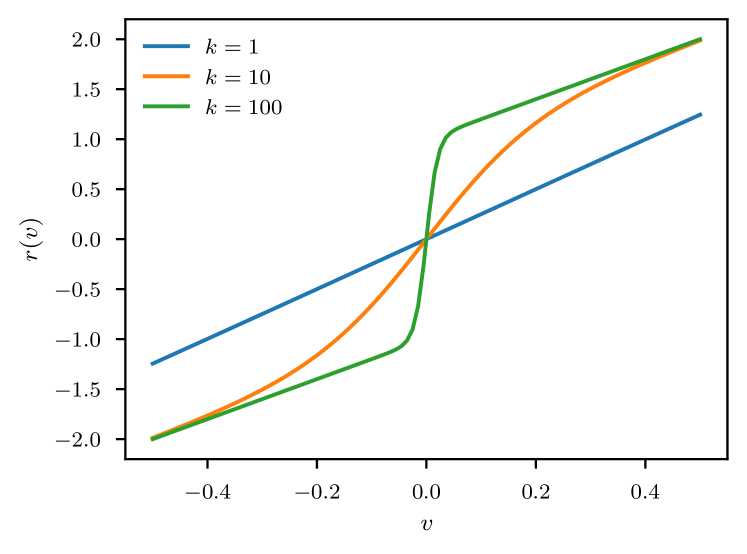
Figure 2: Shape of the $r(v)$ function from (17), with $\alpha=\beta=2$, for various values of $k$.

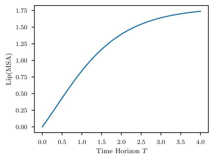
Figure 3: Bounds on the Lipschitz constant of the MSA operator at various time horizons, via Theorem 4.10.

Figure 4: Three successive iterates of the MSA algorithm when ${\rm Lip}(\operatorname{MSA})\leq 0.85$, starting from an initial guess $u^{(0)}(t)=0$.

Consider a nonlinearity of the form

$$r(v)=\alpha v+\beta\left(\frac{1}{1-e^{-kv}}-\frac{1}{2}\right)$$ (17)

so that $d_{\rm min}\triangleq\inf_{v\in\real}r^{\prime}(v)=\alpha$ and $\eta\triangleq\sup_{v\in\real}|r^{\prime\prime}(v)|=\beta k^{2}/(6\sqrt{3})$. Figure 2 illustrates this function for various values of the shape parameter $k$. We select $\alpha=\beta=2$ and $k=4$. Furthermore, we select a target state $x^{*}=(0.1,r(0.1))$, with $u_{\rm max}=2$ and terminal cost weight $\gamma=100$, with model parameters $R=20$, $L=11$, and $C=1$. With these parameters, the contraction rate is $c=1$, and the upper bound on ${\rm Lip}(\operatorname{MSA})$ from Theorem 4.10 is plotted in Figure 3. We select a time horizon of $T=1$, where the bound ${\rm Lip}(\operatorname{MSA})\leq 0.85$ is guaranteed.

In order to implement the MSA algorithm, we use solve_ivp from the SciPy package to integrate the state and costate dynamics. This function implements the explicit Runge-Kutta method RK45, and it approximates the solution as a continuous function using quartic interpolation. Starting with an initial guess of $u^{(0)}=0$, the MSA algorithm quickly converges, with the iterates $u^{(i)}$ for the first three iterations $i\in\{1,2,3\}$ depicted in Figure 4. Note the rapid decay of the $\mathcal{L}_{\infty}$ distance between each successive iterate.

6 Conclusions

In this letter, we have examined an indirect method for the optimal control of strongly contracting systems. We have observed that the time-reversed adjoints of such systems are also contracting with the same rate, with respect to the dual norm, leading to useful bounds on the costate trajectory from PMP. Based on this observation, we bounded the Lipschitz constant of each iteration of MSA, demonstrating that the iteration is actually a contraction mapping for sufficiently strongly contractive systems or for sufficiently short horizons. In these cases, MSA is guaranteed to converge to a unique control that satisfies PMP. With an additional assumption on pointwise uniqueness of the minimizer of the Hamiltonian, we showed that this control is indeed the unique optimal control.

The main approach of this paper, namely using ISS properties of the adjoint to bound the Lipschitz constant of a $\mathcal{U}\to\mathcal{U}$ operator, is quite general and could be applied to many other indirect methods in optimal control. Several variants of MSA, both older [21, 7] and newer [19, 18], could be studied with this type of analysis in future work, possibly with more general convergence criteria. Another practical future direction would be the study of discretized implementation of the forward and backward integration steps, as in [20]. Of course, one could also analyze indirect methods for extensions of the optimal control problem, such as constraints on the terminal state or in the infinite time horizon. An additional interesting direction would be the application of convergence guarantees to model predictive control of contractive nonlinear systems.

7 Proofs

7.1 Proof of Lemma 4

For a general matrix $A\in{}^{n\times n}$, from the definitions of induced norms and dual norms we have

$$\lVert A\rVert_{\star}=\sup_{\lVert y\rVert_{\star}=1}\sup_{\lVert z\rVert\leq 1}z^{\mathsf{T}}Ay$$

Swapping the order of the suprema and applying the definition of the dual norm once again yields

$$\lVert A\rVert_{\star}=\sup_{\lVert z\rVert\leq 1}\sup_{\lVert y\rVert_{\star}=1}y^{\mathsf{T}}A^{\mathsf{T}}z=\sup_{\lVert z\rVert\leq 1}\lVert A^{\mathsf{T}}z\rVert_{\star\star}$$

But ⁿ with any norm is a reflexive Banach space, so $\lVert\cdot\rVert_{\star\star}=\lVert\cdot\rVert$, and thus $\lVert A\rVert_{\star}=\lVert A^{\mathsf{T}}\rVert$. We use this fact to prove both statements. Because $g$ is continuously differentiable and $D_{x}g(x)=D_{x}f(x)^{\mathsf{T}}$,

$${\rm Lip}_{\lVert\cdot\rVert_{\star}}(g)=\sup_{x\in X}\lVert D_{x}g(x)\rVert_{\star}=\sup_{x\in X}\lVert D_{x}f(x)\rVert={\rm Lip}_{\lVert\cdot\rVert}(f)$$

and

$${\rm osL}_{\lVert\cdot\rVert_{\star}}(g) =\sup_{x\in X}\lim_{\alpha\to 0^{+}}\frac{\lVert I_{n}+\alpha D_{x}g(x)\rVert_{\star}-1}{\alpha}$$

$$=\sup_{x\in X}\lim_{\alpha\to 0^{+}}\frac{\lVert I_{n}+\alpha D_{x}f(x)\rVert-1}{\alpha}={\rm osL}_{\lVert\cdot\rVert}(f)$$

7.2 Proof of Lemma 3.7

Let $\bar{x}(t)$ be the trajectory of (3) corresponding to input $\bar{u}(t)=\mathbbold{0}_{k}$. Since (3) is strongly infinitesimally contracting, we can use Lemma 1 to compare a trajectory $x(t)$ with $\bar{x}(t)$:

$$\lVert x(t)-\bar{x}(t)\rVert\leq\frac{\ell_{f,u}}{c}(1-e^{-cT})\!\sup_{\tau\in[0,T]}\!\lVert u(\tau)\rVert_{U}$$

for all $t\in[0,T]$. Since $U$ and $\bar{x}(t)$ are bounded, $x(t)$ is bounded as well. Similarly, the time-reversed costate dynamics (9) have an equilibrium point at the origin when $v(t)=\mathbbold{0}_{n}$, regardless of $x(t)$ and $u(t)$, and (due to Theorem 5) they are strongly contracting with rate $c>0$. Again, we can use Lemma 1 to compare $\lambda^{\leftarrow}(t)$ with the trajectory at the origin:

$$\lVert\lambda^{\leftarrow}(t)\rVert_{\star}\leq\lVert\lambda^{\leftarrow}(0)\rVert_{\star}+\frac{1}{c}(1-e^{-cT})\sup_{\tau\in[0,T]}\lVert v(\tau)\rVert_{\star}$$

for all $t\in[0,T]$. Since $V$ is bounded, $\lambda^{\leftarrow}(t)$ is confined to a ball $\Lambda$ about the origin.

7.3 Proof of Theorem 3.8

As in Theorem 5, let $\lambda^{\leftarrow}(t)=\lambda(T-t)$, so that

$$\frac{d\lambda^{\leftarrow}(t)}{dt}=D_{x}f(T-t,x(T-t),u(T-t))^{\mathsf{T}}\lambda^{\leftarrow}(t)-v(t-T)$$

At any fixed $t$, the $\lambda^{\leftarrow}$ vector field has the Jacobian matrix $D_{x}f(T-t,x(T-t),u(T-t))^{\mathsf{T}}$, which is transpose the Jacobian matrix of $f(T-t,\cdot,u(T-t))$. By Assumption 1, ${\rm osL}(f(T-t,\cdot,u(T-t)))\leq-c$, so Lemma 4 implies that the $\lambda^{\leftarrow}$ vector field is also one-sided Lipschitz with constant $c$, with respect to $\lVert\cdot\rVert_{\star}$. Then we apply Lemma 1 to bound $\lVert\lambda^{\leftarrow}(t)-\bar{\lambda}^{\leftarrow}(t)\rVert_{\star}$ with respect to the inputs $u(t)$, $x(t)$, and $v(t)$, resulting in the following bound on $\lVert\lambda(t)-\bar{\lambda}(t)\rVert_{\star}$:

$$\lVert\lambda(t)-\bar{\lambda}(t)\rVert_{\star}\leq e^{-c(T-t)}\lVert\lambda(T)-\bar{\lambda}(T)\rVert_{\star}$$

$$\qquad\qquad+\ell_{f_{x},u}\int_{t}^{T}e^{-c(\tau-t)}\lVert u(\tau)-\bar{u}(\tau)\rVert_{U}~{}d\tau$$

$$\qquad\qquad+\ell_{f_{x},x}\int_{t}^{T}e^{-c(\tau-t)}\lVert x(\tau)-\bar{x}(\tau)\rVert_{X}~{}d\tau$$

$$\qquad\qquad+\int_{t}^{T}e^{-c(\tau-t)}\lVert v(\tau)-\bar{v}(\tau)\rVert_{\star}~{}d\tau$$

We apply Lemma 1 once more to remove explicit dependence on $x$, via the bound

$$\int_{t}^{T}e^{-c(\tau-t)}\lVert x(\tau)-\bar{x}(\tau)\rVert_{X}~{}d\tau\\ \leq\ell_{f,u}\!\int_{t}^{T}\!\!\!\int_{0}^{\tau}\!\!e^{-c(\tau-t)}e^{-c(\tau-\tau^{\prime})}\lVert u(\tau^{\prime})-\bar{u}(\tau^{\prime})\rVert_{U}~{}d\tau d\tau^{\prime}$$

We then swap the order of integration:

$$\int_{t}^{T}\int_{0}^{\tau} e^{-c(\tau-t)}e^{-c(\tau-\tau^{\prime})}\lVert u(\tau^{\prime})-\bar{u}(\tau^{\prime})\rVert_{U}d\tau^{\prime}d\tau$$

$$=\!\int_{0}^{t}\!\!\int_{t}^{T}\!e^{-c(\tau-t)}e^{-c(\tau-\tau^{\prime})}\lVert u(\tau^{\prime})-\bar{u}(\tau^{\prime})\rVert_{U}d\tau d\tau^{\prime}$$

$$\;\;+\!\int_{t}^{T}\!\!\int_{\tau^{\prime}}^{T}\!e^{-c(\tau-t)}e^{-c(\tau-\tau^{\prime})}\lVert u(\tau^{\prime})-\bar{u}(\tau^{\prime})\rVert_{U}d\tau d\tau^{\prime}$$

$$=\frac{\sinh(c(T-t))}{c}\!\int_{0}^{t}\!e^{-c(T-\tau)}\lVert u(\tau)-\bar{u}\tau)\rVert_{U}d\tau$$

$$\;\;+\frac{e^{-c(T-t)}}{c}\!\int_{t}^{T}\!\sinh(c(T-\tau))\lVert u(\tau)-\bar{u}\tau)\rVert_{U}d\tau$$

7.4 Proof of Corollary 3.9

The first three terms are obvious upper bounds on the first three terms in (LABEL:eq:costate-iss), and

$$\frac{\sinh(c(T\!-\!t))}{c}\!\!\!\int_{0}^{t}\!\!\!e^{-c(T\!-\!\tau)}\;d\tau+\frac{e^{-c(T\!-\!t)}}{c}\!\!\!\int_{t}^{T}\!\!\!\sinh(c(T\!-\!\tau))\;d\tau$$

$$=\!\int_{t}^{T}\!\!\int_{0}^{\tau}\!e^{-c(\tau-t)}e^{-c(\tau-\tau^{\prime})}~{}d\tau^{\prime}d\tau\leq\kappa\!\int_{t}^{T}\!e^{-c(\tau-t)}~{}d\tau\leq\kappa^{2}$$

7.5 Proof of Theorem 4.10

Let $u,\bar{u}\in\mathcal{U}$, and let $x,\bar{x}$ and $\lambda,\bar{\lambda}$ be the corresponding state and costate trajectories. Then for all $t\in[0,T]$,

$$\begin{split}&\lVert\operatorname{MSA}(u)(t)-\operatorname{MSA}(\bar{u})(t)\rVert_{U}\\ &\qquad=\lVert h(t,x(t),\lambda(t))-h(t,\bar{x}(t),\bar{\lambda}(t))\rVert_{U}\\ &\qquad\leq\ell_{h,x}\lVert x(t)-\bar{x}(t)\rVert+\ell_{h,\lambda}\lVert\lambda(t)-\bar{\lambda}(t)\rVert_{\star}\end{split}$$ (18)

The costate dynamics are (9) with $v(t)=-\phi_{x}(t,x(t),u(t))$, which is bounded in $({}^{n},\lVert\cdot\rVert_{\star})$ by the boundedness of $x(t)$ and $u(t)$ and the Lipschitz continuity of $\phi_{x}$. By Corollary 3.9,

$$\lVert\lambda(t)-\bar{\lambda}(t)\rVert_{\star}\leq\lVert\lambda(T)-\bar{\lambda}(T)\rVert_{\star}$$

$$\qquad+\kappa\sup_{t\in[0,T]}\lVert\phi_{x}(t,x(t),u(t))-\phi_{x}(t,\bar{x}(t),\bar{u}(t))\rVert_{\star}$$

$$\qquad+\left(\ell_{f_{x},u}\kappa+\ell_{f_{x},x}\ell_{f,u}\kappa^{2}\right)\sup_{t\in[0,T]}\lVert u(t)-\bar{u}(t)\rVert_{U},$$

where

$$\lVert\lambda(T)-\bar{\lambda}(T)\rVert_{\star}=\lVert\psi_{x}(x(T))-\psi_{x}(\bar{x}(T))\rVert_{\star}$$

$$\leq\ell_{\psi_{x},x}\lVert x(T)-\bar{x}(T)\rVert\leq\ell_{\psi_{x},x}\sup_{t\in[0,T]}\lVert x(t)-\bar{x}(t)\rVert$$

and

$$\lVert\phi_{x}(t,x(t),u(t))-\phi_{x}(t,\bar{x}(t),\bar{u}(t))\rVert_{\star}$$

$$\qquad\leq\ell_{\phi_{x},x}\lVert x(t)-\bar{x}(t)\rVert+\ell_{\phi_{x},u}\lVert u(t)-\bar{u}(t)\rVert_{U}$$

$$\qquad\leq\ell_{\phi_{x},x}\!\!\sup_{t\in[0,T]}\!\lVert x(t)-\bar{x}(t)\rVert\!+\!\ell_{\phi_{x},u}\!\!\sup_{t\in[0,T]}\!\lVert u(t)-\bar{u}(t)\rVert_{U}$$

As a consequence of Lemma 1, $\sup_{t\in[0,T]}\lVert x(t)-\bar{x}(t)\rVert\leq\ell_{f,u}\kappa\sup_{t\in[0,T]}\lVert u(t)-\bar{u}(t)\rVert_{U}$, so we simplify

$$\lVert\lambda(t)-\bar{\lambda}(t)\rVert_{\star}\leq\ell_{\psi_{x},x}\ell_{f,u}\kappa\sup_{t\in[0,T]}\lVert u(t)-\bar{u}(t)\rVert_{U}$$

$$\qquad+\kappa^{2}\ell_{\phi_{x},x}\ell_{f,u}\sup_{t\in[0,T]}\lVert u(t)-\bar{u}(t)\rVert_{U}$$

$$\qquad+\kappa\ell_{\phi_{x},u}\sup_{t\in[0,T]}\lVert u(t)-\bar{u}(t)\rVert_{U}$$

$$\qquad+(\ell_{f_{x},u}\kappa+\ell_{f_{x},x}\ell_{f,u}\kappa^{2})\sup_{t\in[0,T]}\lVert u(t)-\bar{u}(t)\rVert_{U}.$$

Substituting the state and costate difference bounds into (LABEL:eq:fbs-bound) completes the proof of statement (i). Then statement (ii) is a standard consequence of the Banach fixed point theorem.

7.6 Proof of Corollary 4.11

We first establish that the fixed points of the MSA operator are precisely the controls that satisfy PMP. One direction is obvious: $u^{*}=\operatorname{MSA}(u^{*})$ implies that $u^{*}$ satisfies PMP. Now suppose that $u^{*}$ satisfies PMP, and let $x^{*},\lambda^{*}$ be the corresponding state and costate trajectories. Then $u^{*}(t)\in\operatorname*{argmin}_{u\in U}H(t,x^{*}(t),\lambda^{*}(t),u)$ for all $t\in[0,T]$, so the assumption that the Hamiltonian has a unique minimizer implies that $u^{*}(t)=h(t,x^{*}(t),\lambda^{*}(t))$ for all $t\in[0,T]$, and thus $u^{*}=\operatorname{MSA}(u^{*})$.

We then establish that the MSA iteration converges to a unique fixed point $\hat{u}$. For $T$ sufficiently small or $c$ sufficiently large, $\kappa$ is sufficiently small that ${\rm Lip}(\operatorname{MSA})\leq b_{1}\kappa+b_{2}\kappa^{2}<1$, by Theorem 4.10. Then the Banach fixed point theorem establishes that a unique fixed point $\hat{u}$ exists, and that the iteration from any initial guess converges to $\hat{u}$.

Since an optimal control $u^{*}$ exists, it is a fixed point of $\operatorname{MSA}$, and the fixed point of $\operatorname{MSA}$ is unique. Furthermore, if a control $u^{*}$ satisfies PMP, then it is a fixed point of $\operatorname{MSA}$, and hence is equal to the optimal control.

References

- [1] V. V. Aleksandrov. On the accumulation of perturbations in the linear systems with two coordinates. Vestnik MGU, 3:67–76, 1968. (in Russian).
- [2] M. Athans and P. L. Falb. Optimal Control: An Introduction to the Theory and Its Applications. McGraw-Hill, 1966.
- [3] J. T. Betts. Pratical Methods for Optimal Control and Estimation Using Nonlinear Programming. SIAM, 2010.
- [4] L. Böttcher, N. Antulov-Fantulin, and T. Asikis. AI Pontryagin or how artificial neural networks learn to control dynamical systems. Nature communications, 13(1):1–9, 2022. doi:10.1038/s41467-021-27590-0.
- [5] A. Bressan and B. Piccoli. Introduction to the Mathematical Theory of Control. American Institute of Mathematical Sciences, 2007.
- [6] F. Bullo. Contraction Theory for Dynamical Systems. Kindle Direct Publishing, 1.0 edition, 2022. URL: http://motion.me.ucsb.edu/book-ctds.
- [7] F. L. Chernousko and A. A. Lyubushin. Method of successive approximations for solution of optimal control problems. Optimal Control Applications and Methods, 3(2):101–114, 1982. doi:10.1002/oca.4660030201.
- [8] B. A. Conway. A survey of methods available for the numerical optimization of continuous dynamic systems. Journal of Optimization Theory and Applications, 152(2):271–306, 2012. doi:10.1007/s10957-011-9918-z.
- [9] P. E. Crouch, F. Lamnabhi-Lagarrigue, and A. J. van der Schaft. Adjoint and Hamiltonian input-output differential equations. IEEE Transactions on Automatic Control, 40(4):603–615, 1995. doi:10.1109/9.376115.
- [10] W. E. A proposal on machine learning via dynamical systems. Communications in Mathematics and Statistics, 1(5):1–11, 2017. doi:10.1007/s40304-017-0103-z.
- [11] M. Green and D. J. N. Limebeer. Linear Robust Control. Prentice Hall, 1995.
- [12] H. B. Keller. Numerical Methods for Two-Point Boundary-Value Problems. Dover Publications, 2018.
- [13] H. J. Kelley, R. E. Kopp, and H. G. Moyer. Successive approximation techniques for trajectory optimization. Technical report, Grumman Aircraft Engineering Corp, Bethpage NY, 1961. URL: https://apps.dtic.mil/sti/citations/AD0268321.
- [14] H. K. Khalil. Nonlinear Systems. Prentice Hall, 3 edition, 2002.
- [15] O. Kouba and D. S. Bernstein. What is the adjoint of a linear system? [lecture notes]. IEEE Control Systems, 40(3):62–70, 2020. doi:10.1109/MCS.2020.2976389.
- [16] I. A. Krylov and F. L. Chernous'ko. On a method of successive approximations for the solution of problems of optimal control. USSR Computational Mathematics and Mathematical Physics, 2(6):1371–1382, 1963. doi:10.1016/0041-5553(63)90353-7.
- [17] S. Lenhart and J. T. Workman. Optimal Control Applied to Biological Models. Chapman and Hall, 2007.
- [18] Q. Li, L. Chen, C. Tai, and W. E. Maximum principle based algorithms for deep learning. Journal of Machine Learning Research, 18(165):1–29, 2018. URL: http://jmlr.org/papers/v18/17-653.html.
- [19] Q. Li and S. Hao. An optimal control approach to deep learning and applications to discrete-weight neural networks. In International Conference on Machine Learning, pages 2985–2994, 2018. URL: https://proceedings.mlr.press/v80/li18b.html.
- [20] M. McAsey, L. Mou, and W. Han. Convergence of the forward-backward sweep method in optimal control. Computational Optimization and Applications, 53(1):207–226, 2012. doi:10.1007/s10589-011-9454-7.
- [21] S. K. Mitter. Successive approximation methods for the solution of optimal control problems. Automatica, 3(3-4):135–149, 1966. doi:10.1016/0005-1098(66)90009-4.
- [22] A. V. Rao. A survey of numerical methods for optimal control. Advances in the Astronautical Sciences, 135(1):497–528, 2009.
- [23] O. V. Stryk. Numerical solution of optimal control problems by direct collocation. In Optimal Control, pages 129–143. Springer, 1993. doi:10.1007/978-3-0348-7539-4_10.
- [24] P. Tabuada and B. Gharesifard. Universal approximation power of deep residual neural networks through the lens of control. IEEE Transactions on Automatic Control, 2022. doi:10.1109/TAC.2022.3190051.
- [25] D. Zhang, T. Zhang, Y. Lu, Z. Zhu, and B. Dong. You only propagate once: Accelerating adversarial training via maximal principle. Advances in Neural Information Processing Systems, 32, 2019. doi:10.48550/arXiv.1905.00877.