Sanity Check for External Clustering Validation Benchmarks using Internal Validation Measures

Abstract

We address the lack of reliability in benchmarking clustering techniques based on labeled datasets. A standard scheme in external clustering validation is to use class labels as ground truth clusters, based on the assumption that each class forms a single, clearly separated cluster. However, as such cluster-label matching (CLM) assumption often breaks, the lack of conducting a sanity check for the CLM of benchmark datasets casts doubt on the validity of external validations. Still, evaluating the degree of CLM is challenging. For example, internal clustering validation measures can be used to quantify CLM within the same dataset to evaluate its different clusterings but are not designed to compare clusterings of different datasets. In this work, we propose a principled way to generate between-dataset internal measures that enable the comparison of CLM across datasets. We first determine four axioms for between-dataset internal measures, complementing Ackerman and Ben-David’s within-dataset axioms. We then propose processes to generalize internal measures to fulfill these new axioms, and use them to extend the widely used Calinski-Harabasz index for between-dataset CLM evaluation. Through quantitative experiments, we (1) verify the validity and necessity of the generalization processes and (2) show that the proposed between-dataset Calinski-Harabasz index accurately evaluates CLM across datasets. Finally, we demonstrate the importance of evaluating CLM of benchmark datasets before conducting external validation.

1 Introduction

Cluster analysis [1] is an essential exploratory task for data scientists and practitioners in various application domains [2, 3, 4]. It relies on clustering techniques, that is, unsupervised machine learning algorithms that partition the data into subsets called groups or clusters, while maximizing between-cluster separation and within-cluster compactness based on some distance function [5].

Clustering validation measures [6] or quality measures [7] have been proposed to evaluate clustering results. They can be internal or external [8, 5, 1]. Internal validation measures (IVM) give high scores to partitions in which data points with high or low similarities to each other are assigned to the same or different clusters, respectively. In contrast, External validation measures (EVM) quantify how well a clustering matches a ground truth partition. Taking the classes of labeled data as ground truth is a widely used approach to rank clustering techniques on benchmark datasets [6].

Figure 1 illustrates the main issue we propose to address in this work. Using class labels as ground truth in EVM relies on the Cluster-Label Matching (CLM) assumption that the dataset has a good matching between clusters and class labels [9] (Figure 1A). In the worst case, the CLM of the data can be bad with data ranging from having labels randomly assigned to or split between easy-to-detect clusters (Figure 1B), to having labels being well assigned to hard-to-detect clusters (Figure 1J). Then, a low EVM score can be due to a bad clustering of an otherwise good-CLM dataset (Figure 1G) (the clustering technique has low capacity to detect complex clusters) or to a bad-CLM dataset (Figure 1BJ) (the clustering technique may as well have a high capacity (Figure 1CE) or a low one (Figure 1FH), we cannot tell; EVM is unreliable when CLM is bad). Thus, it is crucial to evaluate CLM to measure the intrinsic quality of the ground truth dataset in order to inform and weigh the results of the EVM accordingly (Section 6). Still, the results of EVM over benchmark datasets are often given without considering their CLM [10, 11, 12, 13] casting doubts on the rankings obtained. Here, we aim to evaluate the CLM of labeled datasets.

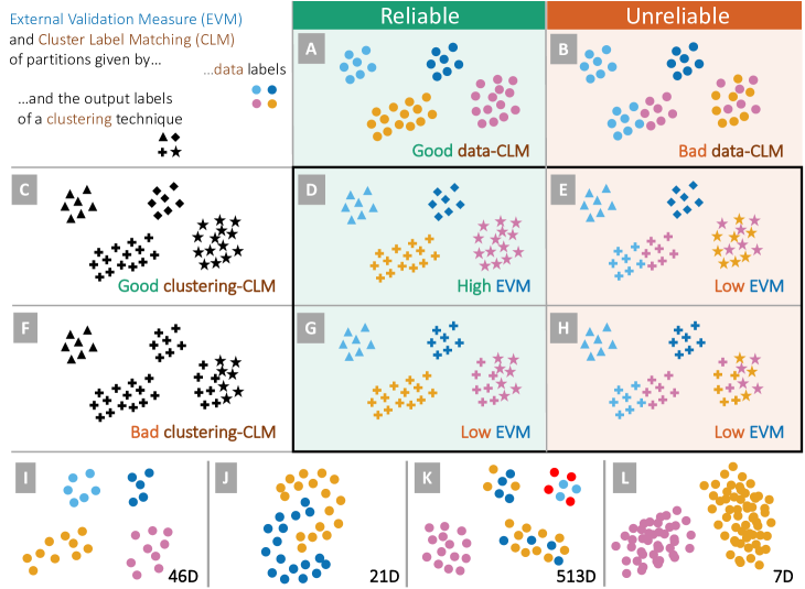
Figure 1: An External Validation Measure (EVM) evaluates the matching between two partitions (markers’ shape and fill) of the same data (D, E, G, H). The Cluster-Label Matching (CLM) is good (A, C) if the partition formed by the labels assigned to the data (shape or fill) matches well the clusters formed by the data point distribution (encoded by position). The labels can be provided with the data (fill) (A, B) or as the output partition of the clustering technique to be evaluated (shape)(C, F). If data-CLM is good (A), the EVM between the data labels (A) and clustering labels (C, F) gives a reliable evaluation (D, G) of the clustering-CLM: high/low EVM (D/G) match with good/bad clustering-CLM (C/F). But if data-CLM is bad (B), the EVM is always low (E, H) and unreliable to evaluate if the clustering-CLM is good (C) or bad (F). It is highly unlikely to get a high EVM (as in D) if the data-CLM is bad (B) as it would mean the clustering technique found by chance the same bad partition as the one given by the data labels (fill (B) and shape (F) would match perfectly in H, not shown). Our main goal is to evaluate and compare data-CLM of several datasets (I,J,K,L) with different characteristics (dimension, size, data and class distributions) to inform clustering evaluation with EVMs. But how can we get CLM scores comparable between datasets?

Yet, evaluating and comparing the CLM of benchmark datasets is challenging. We can use the average EVM scores of several clustering techniques or the accuracy of classifiers in distinguishing classes [14, 15] as a proxy for CLM, but such approaches are not based on principled axioms and are also very time-consuming. In contrast, IVMs are easy to compute, can derive from axioms [7] and could be used as a proxy for CLM, as class partitions forming good clusters would get a higher score. However, they are designed to compare different clustering partitions of a single dataset (Figure 1 C vs F), rather than the class partition of different datasets (Figure 1IJKL). As datasets can differ by their size, dimension, data and class distributions, IVM scores of two labeled datasets cannot be reliably compared, making IVM improper measures of CLM across datasets; such claim is also confirmed by our experiments (Table 1; Table 1). Thus, we lack a proper measure to compare CLM across datasets.

In this research, we propose a set of new axioms from which we derive a between-dataset internal validation measure (IVM_btwn) as a grounded way to assess and compare CLM of different datasets. An IVM_btwn takes a single labeled dataset as input and returns a score evaluating its level of CLM. This score is designed to be comparable across datasets. Our contribution is four-fold:

Axioms We propose four between-dataset axioms that IVM_btwn should satisfy for the fair comparison of CLM, complementing Ackerman and Ben-David’s within-dataset axioms [7] satisfied by standard IVM (i.e., within-dataset IVM; IVM_wthn) (Section 3). These additional axioms require the IVM_btwn to be invariant to the number of data points, classes, and dimensions, and to share a common range.

Generalization process and new between-dataset Calinski Harabasz index From these axioms, we propose technical tricks for generalizing an IVM_wthn into an IVM_btwn. We use them to generalize the Calinski-Harabasz index ($CH$) [16] into a between-dataset $CH$ index ($CH_{btwn}$) (Section 4).

Quantitative evaluations Through an ablation study, we verify the validity and necessity of our generalization process (Section 5.1). We also show that $CH_{btwn}$ ranking 96 real-world datasets significantly outperforms competitors in terms of rank-correlation with the ground truth CLM approximated based on nine clustering techniques, while being up to three orders of magnitude faster to compute than the approximate ground truth (Appendix D). These experiments demonstrate the validity of our axiomatic approach and the effectiveness of $CH_{btwn}$ (Table 1).

Ranking real benchmark data for reliable EVM Lastly, we explain the importance of evaluating CLM in advance of external validation by showing how not doing so adversely affects the conclusions about the comparative performances of clustering techniques (Section 6).

2 Backgrounds and Related Works

Many clustering techniques exist [17], and ensemble approaches have been proposed to combine clustering results to compensate for the weaknesses of individual techniques [18]. Still, it is challenging to define what a good clustering is. For instance, stability is deemed an important criterion [19, 20].

EVM quantify how much the resulting clustering matches with a ground truth partition of the data. For example, Adjusted Mutual Information [21, 22] measures the agreement of two label assignments in terms of information gain corrected for chance effects. Other measures, such as Adjusted Rand Index [23] or V-measure [24], can be used instead.

Classes of labeled datasets have been used extensively as ground truth for clustering EVM [6]. However, despite its potential risk of violating CLM, no principled procedure has yet been proposed to evaluate the reliability of such a ground truth. Our research aims to fill this gap by proposing a measure of CLM. A similar endeavor has been engaged in the supervised learning community to quantify datasets’ difficulty for classification tasks [25].

A natural idea would be to use classification scores as a proxy for CLM [15, 14]. This approach is based on the assumption that the classes of a labeled dataset getting good classification scores will provide a reliable ground-truth for EVM. Still, a classifier is not designed to distinguish well between two "adjacent" classes forming a single cluster (Figure 1B light blue and purple bottom left cluster, good class separation but bad CLM) and two "separated" classes forming distant clusters (Figure 1A light blue and orange clusters, good CLM), nor it is designed to distinguish within-class structures like a class forming a single cluster (Figure 1A light blue class, good CLM) and one made of several distant clusters (Figure 1B light blue class, bad CLM). Moreover, classifiers require expensive training time (Appendix F).

A more direct approach is to average the results of multiple and diverse clustering techniques [18] as their high EVM scores would indicate a good CLM (Figure 1D). However, this approach is computationally expensive too (Appendix F). Moreover, the ground truth it approximates is not based on principled axioms independent of any clustering technique, so it is likely biased in regard to the certain type of clusters these techniques can detect. For lack of a better option, though, we use this approach to get an approximate ground truth in our experiments validating our axiom-based solution, while mitigating the bias by aggregating the EVM scores of multiple clustering techniques.

In contrast to classifiers or clustering techniques, most IVM are relatively inexpensive to compute (Appendix F). Also, as they are based on two criteria—compactness (i.e., the pairwise closeness of data points within a cluster) and separability (i.e., the degree to which clusters lie apart from one another) [5, 26, 27, 8]—they can examine the cluster structure in more details; in Figure 1, an IVM would give a higher score to partitions A and C than to B and F. Moreover, following the axiomatization of clustering by Kleinberg [28], Ackerman and Ben-David [7] proposed four within-dataset axioms that give a common ground to all IVMs: scale invariance, consistency, richness, and isomorphism invariance. These axioms set the requirements a function should satisfy to work properly as an IVM.

Nevertheless, IVMs were originally designed to compare and rank different partitions of the same dataset as shown in Figure 1A-H. Therefore, IVM cannot be used to compare CLM across different datasets in which not only the cluster structure but also the number of points, classes, and dimensions can vary (Figure 1I-L). Here, we propose four additional axioms that an IVM should satisfy to allow this comparison, derive a new IVM satisfying them, and apply it to rank labeled datasets by their reliability to be used as a basis for clustering EVM.

3 New Axioms for Internal Clustering Validation

3.1 Ackerman and Ben-David’s Within-dataset Axioms

Ackerman and Ben-David (A&B) proposed within-dataset axioms [7] that specify the requirements for IVM to properly evaluate clustering partitions. The first axiom is W1: Scale Invariance; it requires measures to be invariant to distance scaling. W2: Consistency is satisfied by a measure that increases when within-cluster compactness or between-cluster separability increases. W3: Richness requires measures to give any fixed cluster partition the best score over the domain by only modifying the distance function. Lastly, W4: Isomorphism Invariance ensures that an IVM does not depend on points identity. Detailed definitions are given in Appendix A.

3.2 Axioms for Enabling Between-dataset Comparison

Within-dataset axioms do not consider the case of comparing scores across datasets; they assume the dataset is invariant. We propose four additional between-dataset axioms that should be satisfied by internal validation measures to allow a fair comparison of cluster partitions across datasets.

Notations We follow the notations used in A&B. We define a finite domain set $X\subset\mathcal{D}$ of dimension $\Delta_{X}$, where $\mathcal{D}$ denotes data space. We denote a clustering partition of $X$ as $C=\{C_{1},C_{2},\cdots,C_{|C|}\}$, where $\forall i\neq j,C_{i}\cap C_{j}=\emptyset$ and $\cup_{i=1}^{|C|}C_{i}=X$. A distance function $d:\mathcal{D}\times\mathcal{D}\rightarrow\mathbb{R}$ is a function that satisfies $d(x,y)\geq 0$, $d(x,y)=d(y,x)$ and $d(x,y)=0$ if $x=y$ for any $x,y\in\mathcal{D}$. If two point sets $X$ and $Y$ follow the same distribution, we say $X\overset{D}{=}Y$. A measure is a function $f$ that takes $C,X,d$ as input and returns a real number. Throughout the section, higher $f$ implies better clustering. Additionally, we define $\underline{W}_{\alpha}$ a random subsample of the set $W$ ($\underline{W}_{\alpha}\overset{D}{=}W$) such that $|\underline{W}_{\alpha}|/|W|=\alpha$, and $\underline{C}_{\alpha}=\{\underline{C_{i}}_{\alpha}\}_{i\in 1\dots|C|}$.

Goals and factors at play IVM_wthn operate on fixed dataset $X$ with possible variations of $C$ and distance $d$. Hence, the number $|C|$ and sizes $|C_{i}|{\forall i}$ of the generated clusters can vary, while $X$ determines a common basis for comparison. A&B’s within-dataset axioms essentially state that the measure $f$ should be invariant to various aspects of the distance $d$. Hence, as $X$ is fixed, $f$ can only vary in relation to the clustering partition $C$. The satisfaction of the A&B’s axioms is a way to ensure IVM_wthn focus on measuring the clustering quality and nothing else.

In contrast, between-dataset IVM (IVM_btwn) shall operate on varying $C$, $d$, and $X$. Imposing IVM_btwn to satisfy A&B’s within-dataset axioms will reduce the influence of $d$. Still several aspects of the varying datasets $X$ now come into play and their influence on IVM_btwn shall be minimized. The sample size $|X|$ is one of them (Axiom B1) and the dimension $\Delta_{X}$ of the data another one (Axiom B2). Moreover, what matters is the matching between natural clusters and data labels more than the number of clusters or labels; therefore, we shall reduce the influence of the number of labels $|C|$ (Axiom B3) imposed by the dataset. Lastly, we need to align IVM_btwn to a comparable range of values (Axiom B4) across datasets, in essence capturing all remaining hard-to-control factors unrelated to clustering quality (i.e., the matching between natural clusters and data labels (CLM)) but integrated by the measure.

Axiom B1 Invariance to the sample size is ensured if subsampling all clusters in the same proportion does not affect the IVM_btwn score, leading to the first axiom:

Data-cardinality Invariance A measure $f$ satisfies data-cardinality invariance if $\forall X,\forall d$ and for every clustering $C$ of $(X,d)$, $f(C,X,d)=f(\underline{C}_{\alpha},X_{\alpha},d)$ with $X_{\alpha}=\cup_{i=1}^{|C|}\underline{C_{i}}_{\alpha}$.

Axiom B2 We shall take into account that data dimension $\Delta_{X}$ may vary across datasets. An important aspect of the dimension called the concentration of distance phenomenon, which is related to the curse of the dimensionality [29], affects the distance measures involved in IVM_btwn. As dimension grows, the variance of data pairwise distances for any distribution tends to be constant while their mean value increases [30, 31, 32]. Therefore, in high dimensional spaces, $d$ will act as a constant function for any data $X$, thus an IVM_btwn $f$ will generate similar scores for all datasets. To mitigate this phenomenon, and as a way to reduce the influence of the dimension, we require the measures to be shift invariant [32, 33] so that the shift of the distances (i.e., growth of the mean) is canceled out:

Shift Invariance A measure $f$ satisfies shift invariance if $\forall X,\forall d$ and for every clustering $C$ over $(X,d)$, $f(C,X,d)=f(C,X,d+\beta)$ $\forall\beta>0$ where $d+\beta$ is a distance function satisfying $(d+\beta)(x,y)=d(x,y)+\beta$, $\forall x,y\in X$.

Axiom B3 The number of classes should not affect an IVM_btwn, for example, two well clustered classes should get an IVM_btwn score as good as 10 well clustered classes. A&B proposed to aggregate class-pairwise IVM_wthn to form other valid IVM_wthn. We follow this principle but state it as an axiom for IVM_btwn:

Class-cardinality Invariance A measure $f$ satisfies class-cardinality invariance if $\forall X,\forall d$ and $\forall C$ over $(X,d)$, $f(C,X,d)=$ $\textrm{agg}_{S\subseteq C,|S|=2}f^{\prime}(S,X,d)$ with $\textrm{agg}_{S}\in\{\textrm{avg}_{S},\min_{S},\max_{S}\}$ and $f^{\prime}$ is an IVM.

By design, $f$ will satisfy all within or between axioms that $f^{\prime}$ satisfies (Appendix B).

Axiom B4 Lastly, we need to ensure that IVM_btwn take a common range of values across datasets, so that their minimum and maximum values correspond to datasets with the worst and the best CLM, respectively, and that these extrema are aligned across datasets (we set them arbitrarily to 0 and 1):

Range Invariance. A measure $f$ satisfies range invariance if $\forall X,\forall d$, and $C$ any clustering over $(X,d)$, $\min_{C}f(C,X,d)=0$ and $\max_{C}f(C,X,d)=1$.

4 Generating Between-dataset Internal Validation Measures

We propose technical tricks to generate IVM_btwn that satisfy our supplementary axioms, and use these tricks to generalize the Calinski-Harabasz index ($CH$) [16] to the between-dataset $CH$ index ($CH_{btwn}$).

4.1 Generalization Tricks for Enabling Between-dataset Comparison

Trick T1: Approaching data-cardinality invariance (B1) We cannot guarantee the invariance of a measure for any subsampling of the data (e.g., very small sample size), but we can get some robustness to random subsampling if we use consistent estimators of population statistics as building blocks of the measure, such as the mean or the median of a class, a pair of classes, or of the whole dataset, or quantities derived from them such as the average distance between all points of two classes.

Trick T2: Achieving shift invariance (B2) Considering a vector of distances $u=(u_{1}\dots u_{n})$, we can define a shift invariant measure by using a ratio of exponential functions $g_{j}(u)=\frac{e^{u_{j}}}{\sum_{k}e^{u_{k}}}$. We observe that $\forall S\in\mathbb{R},g_{j}(u+S)=\frac{e^{u_{j}+S}}{\sum_{k}e^{u_{k}+S}}=\frac{e^{u_{j}}}{\sum_{k}e^{u_{k}}}\frac{e^{S}}{e^{S}}=g_{j}(u)$, hence $g_{j}$ is shift invariant. This trick is at the core of the $t$-SNE loss function [34, 32]. However, $g_{j}$ is not scale-invariant: $\forall\lambda\in\mathbb{R},g_{j}(\lambda u)=\frac{e^{\lambda u_{j}}}{\sum_{k}e^{\lambda u_{k}}}\neq\lambda g_{j}(u)$, hence it will not satisfy axiom W1. We can get back scale-invariance by normalizing each distance $u_{i}$ by a term that scales with all of them together, for example, their standard deviation: $\sigma(u)$. Now $g_{j}(\lambda u/\sigma(\lambda u))=g_{j}(\lambda u/\lambda\sigma(u))=g_{j}(u/\sigma(u))$ is both shift and scale invariant.

Trick T3: Achieving class-cardinality invariance (B3) Class-cardinality invariance can be achieved by following the definition of Axiom B3, such as by defining the measure $f$ as the average of class-pairwise measures.

Trick T4: Achieving range invariance (B4) A common approach to get a unit range for $f$ is to use min-max scaling $f_{u}=(f-f_{\min})/(f_{\max}-f_{\min})$. However, determining the possible minimum and maximum values of $f$ for any data $X$ is not straightforward. Theoretical extrema are usually computed for edge cases far from realistic $X$ and $C$. Wu et al. [35] propose to estimate the worst score over a given dataset $X$ by the expectation $\hat{f}_{\min}=E_{\pi}(f(C^{\pi},X,d))$ of $f$ computed over random partitions $C^{\pi}$ of $(X,d)$ preserving class proportions $|C^{\pi}_{i}|=|C_{i}|{\forall i}$ (Trick 4a)—arguably the worst possible clustering partitions of $X$. In contrast, it is hard to estimate the maximum achievable score over $X$, as this is the very objective of clustering techniques. If the theoretical maximum $f_{\max}$ is known and finite, we propose to use it by default; otherwise, if infinite, we propose to use a logistic function (Trick 4b) to scale it down to $1$ (Note that the scaled measure $f_{u}$ is $0$ if $f_{\max}\rightarrow+\infty$).

4.2 Generalizing the Calinski-Harabasz Index

As a proof-of-concept, we use the proposed tricks to generalize the $CH$ index to the $CH_{btwn}$ index that satisfies both within-dataset (W) and between-dataset (B) axioms. We select $CH$ as it is a representative IVM_wthn [5, 36, 37, 38] widely used for clustering evaluation [39, 40, 41]. It is defined as:

$$CH(C,X,d)=\displaystyle\frac{\sum_{i=1}^{|C|}|C_{i}|d^{2}(c_{i},c)/(|C|-1)}{\sum_{i=1}^{|C|}\sum_{x\in C_{i}}d^{2}(x,c_{i})/(|X|-|C|)},$$

where $c_{i}$ is the centroid of $C_{i}$ and $c$ is the centroid of $X$. A higher value implies a better CLM. The denominator and numerator measure compactness and separability, respectively. Both are estimators of population statistics (Trick 1), reducing by design the influence of data-cardinality (Axiom B1). We get shift invariance (Axiom B2) while preserving scale invariance (Axiom W1) by substituting the square distances by their exponential form normalized by the standard deviation $\sigma_{d}$ of the distances of data points to the centroid (Trick 2), leading to:

$$CH_{1}(C,X,d)=\frac{\sum_{i=1}^{|C|}|C_{i}|e^{d(c_{i},c)/\sigma_{d}}/(|C|-1)}{\sum_{i=1}^{|C|}\sum_{x\in C_{i}}e^{d(x,c_{i})/\sigma_{d}}/(|X|-|C|)}.$$

Then, we apply min-max scaling (Axiom B4). As $\max(CH_{1})=+\infty$, we transform it through a logistic function (Trick 4b) $CH_{2}=1/(1+CH_{1}^{-1})$ so $CH_{2\max}=1$. We estimate the worst score as the expectation of $CH_{2}$ over random clustering partitions $C^{\pi}$ (Trick 4a): $CH_{2\min}=E_{\pi}(CH_{2}(C^{\pi},X,d))$. We get $CH_{3}=(CH_{2}-CH_{2\min})/(CH_{2\max}-CH_{2\min})$.

Lastly, we satisfy class-cardinality (Axiom B3) by averaging class-pairwise scores (Trick 3), which determines the between-cluster Calinski-Harabasz index:

$$CH_{btwn}(C,X,d)=\frac{1}{{|C|\choose 2}}\sum_{S\subseteq C,|S|=2}CH_{3}(S,X,d).$$

Unlike $CH$, which misses all between-dataset axioms except B1, $CH_{btwn}$ satisfies all of them by design, and we prove it also satisfies all within-dataset axioms (Appendix B).

The existence of at least one IVM_btwn provides evidence pointing toward the consistency of our axioms. Still, we cannot prove their completeness nor their soundness for lack of a clear definition of what a good clustering is (See A&B [7] for a discussion of these concepts for clustering). Our experiments validate the importance of these axioms for comparing the CLM of different datasets.

In terms of computational complexity, $CH$, $CH_{1}$, and $CH_{2}$ are $O(|X|\Delta_{X})$, thus $CH_{2\min}=O(|X|\Delta_{X}T)$ while $CH_{2\max}=O(1)$, where $T$ is the number of Monte Carlo simulations to estimate $CH_{2\min}$. Hence, $CH_{3}=O(|X|\Delta_{X}T)$, and finally $CH_{btwn}=O(|X|\Delta_{X}TP_{C})$, where $P_{C}=|C|(|C|+1)/2$ is the number of pairs of classes. Worst-case complexity of $CH_{btwn}$ is linear with all parameters but quadratic with the number of classes, making it very scalable (Appendix F).

5 Evaluation

5.1 Ablation Study of Between-dataset Calinski-Harabasz index

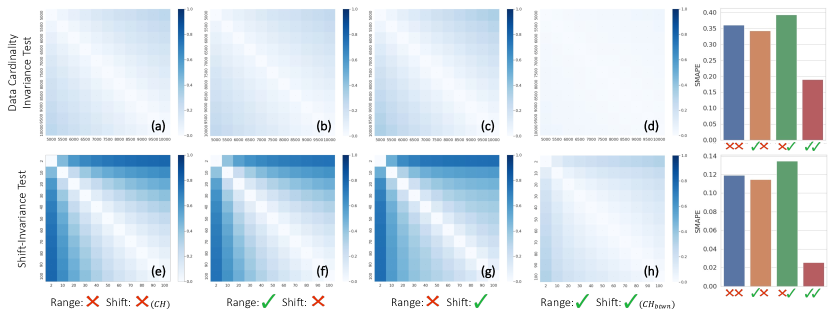
Figure 2: Ablation study of $CH_{btwn}$ (Section 5.1). Heatmaps (a–h) show the SMAPE of $CH_{v}$ variants (each column) for all pairs $(N_{a},N_{b})$ of controlled dataset sizes (top row) and pairs $(\Delta_{a},\Delta_{b})$ of controlled dimensions (bottom row). The lighter the color, the lower the error and the less sensitive $CH_{v}$ to variations of the controlled factor. Bar charts (right) show the average over all pairs of values of controlled factors for each $CH_{v}$ variant. See Appendix H for high-resolution images.

Objectives and design $CH_{btwn}$ derives from $CH$ by using tricks T2, T3, and T4. We want to evaluate the role these tricks play in making IVM_btwn satisfy the new axioms. We consider a synthetic dataset from a previous study [42, 43] made of two bivariate Gaussian clusters (class labels) with various levels of CLM, to which we add noisy dimensions. We consider four variants $CH_{v}$ of $CH_{btwn}$ with shift (T2) and range (T4) tricks switched on or off ($CH_{v}\in\{CH,CH_{T2},CH_{T4},CH_{T2\&T4}=CH_{btwn}\}$). The effect of T1 is not evaluated as B1 is already satisfied by both $CH$ and $CH_{btwn}$, and the effect of T3 is not evaluated because the ground truth synthetic datasets contain only two classes. We control the cardinality (B1) and dimension (B2) of the datasets to evaluate how sensitive $CH_{v}$ variants are to variations of these conditions (the lower, the better). We do not control class-cardinality (B3) as the number of classes (2) is imposed by the available data. Range-invariance (B4) is not controlled as it is imposed by the min-max trick (T4) and not a characteristic of the datasets.

Datasets We prepared 1,000 base datasets $\{X_{1}\dots X_{1000}\}$, each one consisting of $|X|=10,000$ points sampled from two Gaussian clusters ($|C|=2$) within the 2D space and augmented with $98$ noisy dimensions ($\Delta=100$). We controlled the eight independent parameters (ip) of the Gaussians: two covariance matrices (3 ip each), class proportions (1 ip), and the distance between Gaussian means (1 ip), following a previous study [42, 43] (see figure in Appendix C). We add Gaussian noise along the supplementary dimensions, to each cluster-generated data, with a mean 0 and a variance equal to the minimum span of that cluster’s covariance. We generated any dataset $X_{i,t}$ by specifying a triplet $(X_{i},N_{t},\Delta_{t})$ with $X_{i}$ a base dataset, $N_{t}$ the number of data randomly sampled from $X_{i}$ preserving cluster proportions, and $\Delta_{t}$ its dimension where the first two dimensions always correspond to the 2D cluster space. Sensitivity to data-cardinality (B1) (Figure 2 top) For each of the $1000$ base data $X_{i}$, we generated $11$ datasets $X_{i,t}=(X_{i},N_{t},\Delta_{t})_{i\in[1\dots 1000],t\in[0\dots 10]}$ with the controlled data cardinality set to $N_{t}=500t+5000$ and $\Delta_{t}$ drawn uniformly at random from $[2,\dots,100]$. Sensitivity to dimensionality (B2) (Figure 2 bottom) For each of the $1000$ base data $X_{i}$, we generated $11$ datasets $X_{i,t}=(X_{i},N_{t},\Delta_{t})_{i\in[1\dots 1000],t\in[0\dots 10]}$ with $N_{t}$ drawn uniformly at random from $[500,\dots,5000]$ and the controlled dimension set to $\Delta_{0}=2$ or $\Delta_{t}=10t,\forall t>0$.

Measurements For each $CH_{v}$, we compute the matching between a pair ($a,b)$ of values of the controlled factor $t$ (e.g. ($\Delta_{a},\Delta_{b})=(10,30)$) across all $1000$ base data using: $S_{k\in[1\dots 1000]}(CH_{v}(C,X_{k,a},d),CH_{v}(C,X_{k,b},d))$, where S is the Symmetric Mean Absolute Percentage Error (SMAPE) [44] adapted to compare measures with different ranges: ${\displaystyle{S_{k\in K}(F_{k},G_{k})}={\frac{1}{n}}\sum_{k\in K}\frac{|F_{k}-G_{k}|}{|F_{k}|+|G_{k}|}}$ (0 best, 1 worst).

Results Figure 2 shows that all $CH$ variants are slightly sensitive to changes in the data size (a–d), with a larger difference of size leading to bigger errors (off-diagonal darker shades of blue). The average error is about $10\%$ for all variants except $CH_{btwn}$ (top row, blue, orange, and green bars), and $CH_{btwn}$ is five times less sensitive to data cardinality than any other variant (top row, red bar). Regarding dimensionality (e–h), all variants except $CH_{btwn}$ (h) are more strongly affected by larger differences in dimension, with about $35\%$ error on average, while $CH_{btwn}$ (red bar) is slightly below $20\%$ on average, a two-fold improvement over other variants.

The bar chart shows that the combination of both shift invariance (T2) and range invariance (T4) tricks is necessary to get $CH_{btwn}$ satisfying axioms B1 (cardinality invariance) and B2 (shift invariance). It is unexpected, though, that using the shift invariance trick alone makes $CH_{v}$ more sensitive to the dimension. However, this can be explained by the fact that the exponential trick cancels the global shift of all distances (what it is designed for), disregarding the effect on the range of the IVM itself (a non-linear aggregation of distances), a factor that is then mitigated by the range trick (T4).

5.2 Between-dataset Rank Correlation Analysis

Spearman’s rank correlation		GT-ranking EVMs
with approximate ground truth CLM		ami	arand	vm	nmi
Classifiers	SVM	0.5427	0.6235	0.4625	0.4827
	$k$NN	0.4876	0.5810	0.3974	0.4094
	MLP	0.4405	0.5386	0.3600	0.3761
	NB	0.4126	0.5276	0.3157	0.3130
	RF	0.4893	0.5741	0.3991	0.3889
	LR	0.4456	0.5382	0.3666	0.3873
	LDA	0.4999	0.5726	0.3945	0.3606
	Ensemble	0.5922	0.6748	0.4614	0.4099
IVMwthn	Silhouette	0.5648	0.6800	0.4549	0.4208
	Xie-Beni	0.6201	∗0.7019	0.4934	0.4446
	Dunn	0.4026	0.3534	0.5366	∗0.5979
	I Index	0.5668	0.5957	∗∗0.6086	∗∗0.6454
	Davies-Bouldin	∗∗0.7091	∗∗0.7513	∗0.5719	0.5015
	$CH$	∗0.5923	0.6222	0.4487	0.3810
IVMbtwn (ours)	$CH_{btwn}$	∗∗∗0.7893	∗∗∗0.7981	∗∗∗0.7022	∗∗∗0.6561
∗∗∗, ∗∗, ∗: first, second, and third highest scores for each EVM
Every result was validated to be statistically significant ($p<.001)$ through Spearman’s rank correlation test.

Table 1: Rank correlations between approximate ground truth CLM ranking based on 9 clustering techniques and estimated CLM ranking obtained by $CH_{btwn}$, various IVM_wthn, and classifiers. $CH_{btwn}$ rankings (***) outperform all the competitors and achieved an improvement of about 20% compared to its within-dataset version ($CH$).

Objectives and design We assess $CH_{btwn}$ against competitors for best estimating the CLM ranking of publicly available labeled datasets. We approximate a ground truth CLM quality for each labeled dataset using multiple clustering techniques. We then compare the rankings made by all competitors and $CH_{btwn}$ to this ground truth using Spearman’s rank correlation.

Datasets We collected 96 publicly available labeled datasets with diverse numbers of data points, class labels, cluster patterns (presumably), and dimensionality (Appendix E).

Approximating the ground truth CLM For lack of definite ground truth clusters in multidimensional real data, we used the maximum EVM score achievable by nine various clustering techniques on a labeled dataset as an approximation of the ground truth (GT) CLM score for that dataset. These GT scores were used to get the GT-ranking of all the datasets. This scheme relies on the fact that high EVM implies good CLM (Section 1; Figure 1 A and D). We used Bayesian optimization [45] to find the best hyperparameter setting for each clustering technique. We obtained GT-ranking based on four EVMs: adjusted rand index (arand) [23], adjusted mutual information (ami) [22], V-measure (vm) [24], and normalized mutual information (nmi) [46] with geometric mean. For clustering techniques, we used HDBSCAN [47], DBSCAN [48], $K$-Means [49], $K$-Medoids [50], $X$-Means [51], Birch [52], and Single, Average, and Complete variants of Agglomerative Clustering [53] (Appendix D).

Competitors We compared supervised classifiers, IVM_wthn, and $CH_{btwn}$ to the GT ranking. For classifiers, we used SVM, $k$NN, Multilayer Perceptron (MLP), Naive Bayesian Networks (NB), Random Forest (RF), Logistic Regression (LR), Linear Discriminant Analysis (LDA), and their ensembles; the selected classifiers are the ones used for evaluating clustering in Rodríguez et al. [14]. We measured the classification score of a given labeled dataset, using five-fold cross validation and Bayesian optimization [45] to find the best hyperparameter setting. The accuracy in predicting class labels was averaged over the five validation sets to get a proxy of the CLM score for that dataset. For the ensemble method, we got the proxy as the highest accuracy score among the seven classifiers for each dataset independently. Regarding IVM_wthn, we considered the list of Liu et al. [5], except the ones optimized based on the elbow rule (e.g., Modified Hubert $\Gamma$ statistic [54]) and the ones requiring several clustering results (e.g., S_Dbw index [55]), thus we used: $CH$, Davies-Bouldin index [56], Dunn index [57], I index [37], Silhouette [58], and Xie-Beni index [59] (See details in Appendix D).

Results Table 1 shows that for every EVM, $CH_{btwn}$ (***) outperforms all competitors. Especially, $CH_{btwn}$ achieved a performance improvement of about 20% compared to $CH$. The second (**) and third (*) places vary depending on the EVM, but they are all part of the IVM_wthn category. Therefore, $CH_{btwn}$ can be used as a reliable measure of CLM to rank datasets (Figure 3) despite their drastic variations in terms of dimension, number of class labels, and data size. It also runs far faster than optimizing any of the GT clustering techniques (tens of seconds versus several hours for all 96 datasets; Appendix F), clearly demonstrating its benefit both in terms of time and accuracy.

6 Application: Ranking the Labeled Datasets for Reliable EVM

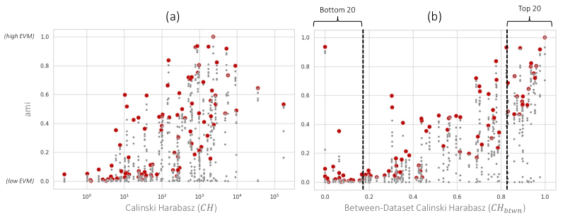
Figure 3: All (gray points) and best (red points) ami scores of GT clustering techniques for the $96$ benchmark datasets, ranked by $CH$ (left) and $CH_{btwn}$ (right). The top $20$ datasets in terms of $CH_{btwn}$ (right) are the most reliable to evaluate and compare clustering techniques using EVMs.

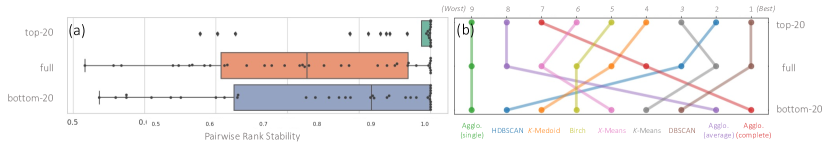
Figure 4: (a) Distribution of pairwise rank stability for bottom-20 (blue; $\mathcal{P}^{-}$), full (orange; $\mathcal{P}^{*}$), and top-20 (green; $\mathcal{P}^{+}$) datasets. (b) Rankings of clustering techniques for each set. All rankings are based on ami EVM averaged over the datasets within each set. Using the datasets top-ranked by $CH_{btwn}$ as a proxy of their good CLM leads to stable and reliable rankings ((a) green bar).

Objectives and design We want to demonstrate the importance of evaluating the CLM of benchmark datasets prior to conducting the external validation of clustering techniques. Here, in addition to the full set of $96$ public datasets ($\mathcal{P}^{*}$), we consider the top-20 ($\mathcal{P}^{+}$) and bottom-20 ($\mathcal{P}^{-}$) datasets as per their $CH_{btwn}$ rank (Figure 3b) (the top-20 and bottom-20 datasets are given in Appendix C).

We consider simulating the situation where a data scientist would arbitrarily choose $10$ benchmark datasets ($\mathcal{B}$) among the datasets at hand for the task T of ranking clustering techniques according to $EVM_{\mathcal{B}}$, the average EVM over $\mathcal{B}$. For each $\mathcal{P}\in\{\mathcal{P}^{+},\mathcal{P}^{*},\mathcal{P}^{-}\}$, we simulate $100$ times picking $\mathcal{B}$ at random among $\mathcal{P}$. For each $\mathcal{P}$, we measure the pairwise rank stability $P_{\mathcal{B}}(A,B)=\max(1-p,p)$ of clustering techniques A and B over $\mathcal{B}$ by counting the proportion $p$ of cases $\texttt{ami}_{\mathcal{B}}(A)>\texttt{ami}_{\mathcal{B}}(B)$.

Assumptions We expect that conducting T on any subset of good-CLM datasets would provide similar rankings (Figure 1A) where pairwise ranks remain stable ($\forall(A,B),P_{\mathcal{B}}(A,B)\approx 1$), whereas conducting T using bad-CLM datasets would lead to arbitrary and unstable rankings ($\forall(A,B),P_{\mathcal{B}}(A,B)$ spread over $[0.5,1]$) (Figure 1BEH).

Results and discussion Figure 4a shows that pairwise ranks stay stable only in $\mathcal{P}^{+}$, which verifies our assumptions. Moreover, we found that the rankings of clustering techniques made by $EVM_{\mathcal{P^{+}}}$, $EVM_{\mathcal{P^{*}}}$, and $EVM_{\mathcal{P^{-}}}$ are completely different (Figure 4b). Still, some datasets within $\mathcal{P}^{-}$ (e.g., Spambase, Hepatitis [60]) have been used for external clustering validation in previous studies [10, 11, 12, 13] without CLM evaluation, casting doubt on their conclusion and showing this issue shall gain more attention in the benchmarking community. CLM scores could be used further to inform benchmarking results (Appendix G) or to improve dataset’s reliability by modifying datasets’ class labels.

7 Conclusion

In this research, we provided a grounded way to evaluate the reliability of benchmark labeled datasets used for the external evaluation of clustering techniques. We proposed to measure their level of cluster-label matching (CLM). We presented four between-dataset axioms and technical tricks to generate measures that satisfy them. We used these tricks to design a new between-dataset internal validation measure $CH_{btwn}$ generalizing the Calinski-Harabasz index for across-datasets comparisons. We studied the accuracy of this measure to rank $96$ benchmark datasets and showed that it outperforms all competitors in terms of time and accuracy. We demonstrated its usefulness in determining the most reliable datasets for comparing clustering techniques.

As future work, we want to explore further the use of our tricks to generalize other IVM_wthn, and explore how to use the CLM score to build better clustering benchmarks.

References

- [1] Anil K Jain and Richard C Dubes. Algorithms for clustering data. Prentice-Hall, Inc., 1988.
- [2] Sehi L’Yi, Bongkyung Ko, DongHwa Shin, Young-Joon Cho, Jaeyong Lee, Bohyoung Kim, and Jinwook Seo. Xclusim: a visual analytics tool for interactively comparing multiple clustering results of bioinformatics data. BMC bioinformatics, 16(11):1–15, 2015.
- [3] Satu Elisa Schaeffer. Graph clustering. Computer Science Review, 1(1):27–64, 2007.
- [4] Mathilde Caron, Piotr Bojanowski, Armand Joulin, and Matthijs Douze. Deep clustering for unsupervised learning of visual features. In Proceedings of the European Conference on Computer Vision (ECCV), September 2018.
- [5] Yanchi Liu, Zhongmou Li, Hui Xiong, Xuedong Gao, and Junjie Wu. Understanding of internal clustering validation measures. In 2010 IEEE International Conference on Data Mining, pages 911–916, 2010.
- [6] Ines Färber, Stephan Günnemann, Hans-Peter Kriegel, Peer Kröger, Emmanuel Müller, Erich Schubert, Thomas Seidl, and Arthur Zimek. On using class-labels in evaluation of clusterings. In MultiClust: 1st international workshop on discovering, summarizing and using multiple clusterings held in conjunction with KDD, page 1, 2010.
- [7] Shai Ben-David and Margareta Ackerman. Measures of clustering quality: A working set of axioms for clustering. In D. Koller, D. Schuurmans, Y. Bengio, and L. Bottou, editors, Advances in Neural Information Processing Systems, volume 21. Curran Associates, Inc., 2008.
- [8] Eréndira Rendón, Itzel M Abundez, Citlalih Gutierrez, Sergio Díaz Zagal, Alejandra Arizmendi, Elvia M Quiroz, and H Elsa Arzate. A comparison of internal and external cluster validation indexes. In Proceedings of the 2011 American Conference, San Francisco, CA, USA, volume 29, pages 1–10, 2011.
- [9] Michaël Aupetit. Sanity check for class-coloring-based evaluation of dimension reduction techniques. In Proceedings of the Fifth Workshop on Beyond Time and Errors: Novel Evaluation Methods for Visualization, BELIV ’14, page 134–141, New York, NY, USA, 2014. Association for Computing Machinery.
- [10] Hajar Rehioui, Abdellah Idrissi, Manar Abourezq, and Faouzia Zegrari. Denclue-im: A new approach for big data clustering. Procedia Computer Science, 83:560–567, 2016. The 7th International Conference on Ambient Systems, Networks and Technologies (ANT 2016) / The 6th International Conference on Sustainable Energy Information Technology (SEIT-2016) / Affiliated Workshops.
- [11] Md. Kafi Khan, Sakil Sarker, Syed Mahmud Ahmed, and Mozammel H A Khan. K-cosine-means clustering algorithm. In 2021 International Conference on Electronics, Communications and Information Technology (ICECIT), pages 1–4, 2021.
- [12] Nicholas Monath, Ari Kobren, Akshay Krishnamurthy, and Andrew McCallum. Gradient-based hierarchical clustering. In 31st Conference on neural information processing systems (NIPS 2017), Long Beach, CA, USA, 2017.
- [13] Nicholas Monath, Manzil Zaheer, Daniel Silva, Andrew McCallum, and Amr Ahmed. Gradient-based hierarchical clustering using continuous representations of trees in hyperbolic space. In Proceedings of the 25th ACM SIGKDD International Conference on Knowledge Discovery & Data Mining, KDD ’19, page 714–722, New York, NY, USA, 2019. Association for Computing Machinery.
- [14] Jorge Rodríguez, Miguel Angel Medina-Pérez, Andres Eduardo Gutierrez-Rodríguez, Raúl Monroy, and Hugo Terashima-Marín. Cluster validation using an ensemble of supervised classifiers. Knowledge-Based Systems, 145:134–144, 2018.
- [15] O. Abul, A. Lo, R. Alhajj, F. Polat, and K. Barker. Cluster validity analysis using subsampling. In SMC’03 Conference Proceedings. 2003 IEEE International Conference on Systems, Man and Cybernetics. Conference Theme - System Security and Assurance (Cat. No.03CH37483), volume 2, pages 1435–1440 vol.2, 2003.
- [16] T. Caliński and J Harabasz. A dendrite method for cluster analysis. Communications in Statistics, 3(1):1–27, 1974.
- [17] Dongkuan Xu and Yingjie Tian. A comprehensive survey of clustering algorithms. Annals of Data Science, 2(2):165–193, 2015.
- [18] Sandro Vega-Pons and José Ruiz-Shulcloper. A survey of clustering ensemble algorithms. International Journal of Pattern Recognition and Artificial Intelligence, 25(03):337–372, 2011.
- [19] Ulrike Von Luxburg. Clustering stability: an overview. 2010.
- [20] Shai Ben-David, Ulrike von Luxburg, and Dávid Pál. A sober look at clustering stability. In International conference on computational learning theory, pages 5–19. Springer, 2006.
- [21] Alexander Strehl and Joydeep Ghosh. Cluster ensembles—a knowledge reuse framework for combining multiple partitions. Journal of machine learning research, 3(Dec):583–617, 2002.
- [22] Nguyen Xuan Vinh, Julien Epps, and James Bailey. Information theoretic measures for clusterings comparison: Variants, properties, normalization and correction for chance. The Journal of Machine Learning Research, 11:2837–2854, 2010.
- [23] Jorge M. Santos and Mark Embrechts. On the use of the adjusted rand index as a metric for evaluating supervised classification. In Cesare Alippi, Marios Polycarpou, Christos Panayiotou, and Georgios Ellinas, editors, Artificial Neural Networks – ICANN 2009, pages 175–184, Berlin, Heidelberg, 2009. Springer Berlin Heidelberg.
- [24] Andrew Rosenberg and Julia Hirschberg. V-measure: A conditional entropy-based external cluster evaluation measure. In Proceedings of the 2007 joint conference on empirical methods in natural language processing and computational natural language learning (EMNLP-CoNLL), pages 410–420, 2007.
- [25] Kawin Ethayarajh, Yejin Choi, and Swabha Swayamdipta. Understanding dataset difficulty with -usable information. In Kamalika Chaudhuri, Stefanie Jegelka, Le Song, Csaba Szepesvari, Gang Niu, and Sivan Sabato, editors, Proceedings of the 39th International Conference on Machine Learning, volume 162 of Proceedings of Machine Learning Research, pages 5988–6008. PMLR, 17–23 Jul 2022.
- [26] Pang-Ning Tan, Michael Steinbach, and Vipin Kumar. Introduction to data mining, addison. ed: Boston, MA USA: Wesley Longman, Publishing Co., Inc, 2005.
- [27] Ying Zhao and George Karypis. Evaluation of hierarchical clustering algorithms for document datasets. In Proceedings of the Eleventh International Conference on Information and Knowledge Management, CIKM ’02, page 515–524, New York, NY, USA, 2002. Association for Computing Machinery.
- [28] Jon Kleinberg. An impossibility theorem for clustering. In S. Becker, S. Thrun, and K. Obermayer, editors, Advances in Neural Information Processing Systems, volume 15. MIT Press, 2002.
- [29] Richard Bellman. Dynamic programming. Science, 153(3731):34–37, 1966.
- [30] Kevin Beyer, Jonathan Goldstein, Raghu Ramakrishnan, and Uri Shaft. When is “nearest neighbor” meaningful? In International conference on database theory, pages 217–235. Springer, 1999.
- [31] Damien Francois, Vincent Wertz, and Michel Verleysen. The concentration of fractional distances. IEEE Transactions on Knowledge and Data Engineering, 19(7):873–886, 2007.
- [32] John A. Lee and Michel Verleysen. Shift-invariant similarities circumvent distance concentration in stochastic neighbor embedding and variants. Procedia Computer Science, 4:538–547, 2011. Proceedings of the International Conference on Computational Science, ICCS 2011.
- [33] John A. Lee and Michel Verleysen. Two key properties of dimensionality reduction methods. In 2014 IEEE Symposium on Computational Intelligence and Data Mining (CIDM), pages 163–170, 2014.
- [34] Laurens Van der Maaten and Geoffrey Hinton. Visualizing data using t-sne. Journal of machine learning research, 9(11), 2008.
- [35] Junjie Wu, Hui Xiong, and Jian Chen. Adapting the right measures for k-means clustering. In Proceedings of the 15th ACM SIGKDD International Conference on Knowledge Discovery and Data Mining, KDD ’09, page 877–886, New York, NY, USA, 2009. Association for Computing Machinery.
- [36] Yanchi Liu, Zhongmou Li, Hui Xiong, Xuedong Gao, Junjie Wu, and Sen Wu. Understanding and enhancement of internal clustering validation measures. IEEE Transactions on Cybernetics, 43(3):982–994, 2013.
- [37] U. Maulik and S. Bandyopadhyay. Performance evaluation of some clustering algorithms and validity indices. IEEE Transactions on Pattern Analysis and Machine Intelligence, 24(12):1650–1654, 2002.
- [38] Hui Xiong and Zhongmou Li. Clustering validation measures., 2013.
- [39] Xu Wang and Yusheng Xu. An improved index for clustering validation based on silhouette index and calinski-harabasz index. IOP Conference Series: Materials Science and Engineering, 569(5):052024, jul 2019.
- [40] Szymon Łukasik, Piotr A. Kowalski, Małgorzata Charytanowicz, and Piotr Kulczycki. Clustering using flower pollination algorithm and calinski-harabasz index. In 2016 IEEE Congress on Evolutionary Computation (CEC), pages 2724–2728, 2016.
- [41] Jonathan Baarsch and M Emre Celebi. Investigation of internal validity measures for k-means clustering. In Proceedings of the international multiconference of engineers and computer scientists, volume 1, pages 14–16. sn, 2012.
- [42] Mostafa M. Abbas, Michaël Aupetit, Michael Sedlmair, and Halima Bensmail. Clustme: A visual quality measure for ranking monochrome scatterplots based on cluster patterns. Computer Graphics Forum, 38(3):225–236, 2019.
- [43] Michaël Aupetit, Michael Sedlmair, Mostafa M. Abbas, Abdelkader Baggag, and Halima Bensmail. Toward perception-based evaluation of clustering techniques for visual analytics. In 30th IEEE Visualization Conference, IEEE VIS 2019 - Short Papers, Vancouver, BC, Canada, October 20-25, 2019, pages 141–145. IEEE, 2019.
- [44] Chris Tofallis. A better measure of relative prediction accuracy for model selection and model estimation. Journal of the Operational Research Society, 66(8):1352–1362, 2015.
- [45] Jasper Snoek, Hugo Larochelle, and Ryan P Adams. Practical bayesian optimization of machine learning algorithms. In F. Pereira, C.J. Burges, L. Bottou, and K.Q. Weinberger, editors, Advances in Neural Information Processing Systems, volume 25. Curran Associates, Inc., 2012.
- [46] Alexander Strehl and Joydeep Ghosh. Cluster ensembles—a knowledge reuse framework for combining multiple partitions. Journal of machine learning research, 3(Dec):583–617, 2002.
- [47] Ricardo J. G. B. Campello, Davoud Moulavi, and Joerg Sander. Density-based clustering based on hierarchical density estimates. In Jian Pei, Vincent S. Tseng, Longbing Cao, Hiroshi Motoda, and Guandong Xu, editors, Advances in Knowledge Discovery and Data Mining, pages 160–172, Berlin, Heidelberg, 2013. Springer Berlin Heidelberg.
- [48] Erich Schubert, Jörg Sander, Martin Ester, Hans Peter Kriegel, and Xiaowei Xu. Dbscan revisited, revisited: Why and how you should (still) use dbscan. ACM Trans. Database Syst., 42(3), jul 2017.
- [49] John A Hartigan and Manchek A Wong. Algorithm as 136: A k-means clustering algorithm. Journal of the royal statistical society. series c (applied statistics), 28(1):100–108, 1979.
- [50] Hae-Sang Park and Chi-Hyuck Jun. A simple and fast algorithm for k-medoids clustering. Expert Systems with Applications, 36(2, Part 2):3336–3341, 2009.
- [51] Dan Pelleg, Andrew W Moore, et al. X-means: Extending k-means with efficient estimation of the number of clusters. In Icml, volume 1, pages 727–734, 2000.
- [52] Tian Zhang, Raghu Ramakrishnan, and Miron Livny. Birch: An efficient data clustering method for very large databases. In Proceedings of the 1996 ACM SIGMOD International Conference on Management of Data, SIGMOD ’96, page 103–114, New York, NY, USA, 1996. Association for Computing Machinery.
- [53] Daniel Müllner. Modern hierarchical, agglomerative clustering algorithms. arXiv preprint arXiv:1109.2378, 2011.
- [54] Lawrence Hubert and Phipps Arabie. Comparing partitions. Journal of classification, 2(1):193–218, 1985.
- [55] M. Halkidi and M. Vazirgiannis. Clustering validity assessment: finding the optimal partitioning of a data set. In Proceedings 2001 IEEE International Conference on Data Mining, pages 187–194, 2001.
- [56] David L. Davies and Donald W. Bouldin. A cluster separation measure. IEEE Transactions on Pattern Analysis and Machine Intelligence, PAMI-1(2):224–227, 1979.
- [57] Joseph C Dunn. Well-separated clusters and optimal fuzzy partitions. Journal of cybernetics, 4(1):95–104, 1974.
- [58] Peter J. Rousseeuw. Silhouettes: A graphical aid to the interpretation and validation of cluster analysis. Journal of Computational and Applied Mathematics, 20:53–65, 1987.
- [59] Xuanli Lisa Xie and Gerardo Beni. A validity measure for fuzzy clustering. IEEE Transactions on pattern analysis and machine intelligence, 13(8):841–847, 1991.
- [60] Arthur Asuncion and David Newman. Uci machine learning repository, 2007.